Structural XML Classi cation in Concept Drifting Data Streams · Structural XML Classi cation in...

Structural XML Classification in Concept Drifting Data Streams 1

Structural XML Classification in ConceptDrifting Data Streams

Dariusz BRZEZINSKI

Institute of Computing Science, Poznan University of Technologyul. Piotrowo 2, 60–965 Poznan, Poland

[email protected]

Maciej PIERNIK

Institute of Computing Science, Poznan University of Technologyul. Piotrowo 2, 60–965 Poznan, Poland

[email protected]

Abstract Classification of large, static collections of XML data has

been intensively studied in the last several years. Recently however, the

data processing paradigm is shifting from static to streaming data, where

documents have to be processed online using limited memory and class

definitions can change with time in an event called concept drift. As

most existing XML classifiers are capable of processing only static data,

there is a need to develop new approaches dedicated for streaming envi-

ronments. In this paper, we propose a new classification algorithm for

XML data streams called XSC. The algorithm uses incrementally mined

frequent subtrees and a tree-subtree similarity measure to classify new

documents in an associative manner. The proposed approach is experi-

mentally evaluated against eight state-of-the-art stream classifiers on real

and synthetic data. The results show that XSC performs significantly

better than competitive algorithms in terms of accuracy and memory

usage.

Keywords XML, Data Stream, Classification, Concept Drift, Tree-

edit Distance

2 Maciej PIERNIK

§1 IntroductionIn the past few years, several data mining algorithms have been pro-

posed to discover knowledge from XML data 29). However, these algorithms

were almost exclusively analyzed in the context of static datasets, while in many

new applications one faces the problem of processing massive data volumes in

the form of transient data streams. Example applications involving processing

XML data generated at very high rates include monitoring messages exchanged

by web-services, management of complex event streams, distributed ETL pro-

cesses, and publish/subscribe services for RSS feeds 25).

The processing of streaming data implies new requirements concerning

limited amount of memory, short processing time, and single scan of incoming

examples, none of which are sufficiently handled by traditional XML data mining

algorithms. Furthermore, due to the nonstationary nature of data streams,

target concepts tend to change over time in an event called concept drift. Concept

drift occurs when the concept about which data is being collected shifts from

time to time after a minimum stability period 17). Drifts can be reflected by class

assignment changes, attribute distribution changes, or an introduction of new

classes (concept evolution), all of which deteriorate the accuracy of algorithms.

Although several general-purpose data stream classifiers have been pro-

posed 17), they do not take into account the semi-structural nature of XML.

On the other hand, XML-specific classifiers such as XRules 36) or X-Class 11) are

designed to handle only static data. To the best of our knowledge, the only avail-

able XML stream classifier has been proposed by Bifet and Gavalda 4). However,

this proposal focuses only on incorporating incremental subtree mining to the

learning process and, therefore, does not fully utilize the structural similarities

between XML documents. Furthermore, the classification method proposed by

Bifet and Gavalda is only capable of dealing with sudden concept drifts, but will

not react to gradual drift, attribute changes, or concept evolution.

In this paper, we propose the XML Stream Classifier (XSC), a stream

classification algorithm, which employs incremental subtree mining and partial

tree-edit distance to classify XML documents online. By dynamically creating

separate models for each class, the proposed method is capable of dealing with

concept evolution and gradual drift. Moreover, XSC can be trained like a cost

sensitive learner and handle skewed class distributions. We will show that the

resulting system performs favorably when compared with competitive stream

classifiers, additionally being able to cope with different types of concept drift.


This work extends the study conducted in 7), which presented a pre-

liminary version of XSC. Differently from our previous work, we provide a more

in-depth analysis of the proposed algorithm and introduce several enhancements:

i) a clear distinction between synchronous and asynchronous training is made

and the differences between the two approaches are experimentally evaluated;

ii) we analyze three additional vote weighting functions, which are taken into

account in the final algorithm; iii) a separate analysis concerning duplicate pat-

tern treatment is added to explain its importance to the proposed classifier; iv)

to assess the applicability of our approach, we conduct an experimentation with

more concept-drifting datasets involving additional types of drift and compare

our algorithm with a wider range of state-of-the-art data stream classifiers.

The paper is structured as follows. Section 2 provides basic definitions

and notation while Section 3 presents related work. In Section 4, we introduce

a new incremental XML classification algorithm, which uses maximal frequent

subtrees and partial tree-edit distance to perform predictions. Furthermore,

we analyze possible variations of the proposed algorithm for different stream

settings. The algorithm is later experimentally evaluated on real and synthetic

datasets in Section 5. Finally, in Section 6 we draw conclusions and discuss lines

of future research.

§2 Basic Concepts and NotationIn static classification problems, a set of learning examples contains pairs

{d, y}, where d is an XML document and y is a class label, which falls into one of

several categorical values (y ∈ C). Based on all learning examples, the learning

algorithm constructs a classifier, which is capable of predicting class labels of

previously unseen examples.

In data stream classification problems, examples arrive continuously in

the form of a potentially infinite stream S. A learning algorithm is presented

with a sequence of labeled examples st = {dt, yt} for t = 1, 2, . . . , T . At each time

step t, a learner can analyze only a limited portion of historical labeled training

examples (st−∆, . . . , st−1, st) and an incoming instance st+1, which is treated as

a testing example. Generally, examples can be read from a data stream either

incrementally (online) or in portions (blocks). In the first approach, algorithms

process single examples appearing one by one in consecutive moments in time,

while in the second approach, examples are available only in larger sets called

data blocks (or data chunks). Blocks B1, B2, . . . , Bi are usually of equal size and

4 Maciej PIERNIK

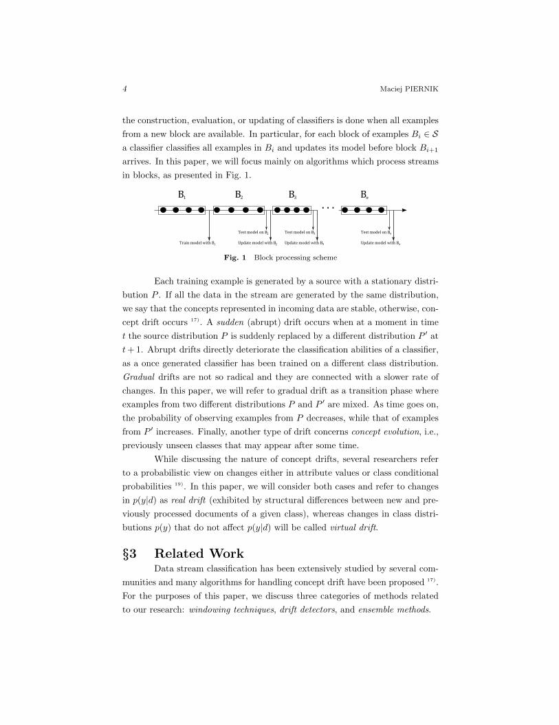
the construction, evaluation, or updating of classifiers is done when all examples

from a new block are available. In particular, for each block of examples Bi ∈ Sa classifier classifies all examples in Bi and updates its model before block Bi+1

arrives. In this paper, we will focus mainly on algorithms which process streams

in blocks, as presented in Fig. 1.

B1

. . .B2 B3 Bn

Test model on B

Update model with BTrain model with B

Test model on B

Update model with B

Test model on B

Update model with B1

2 n

2 3

3

n

Fig. 1 Block processing scheme

Each training example is generated by a source with a stationary distri-

bution P . If all the data in the stream are generated by the same distribution,

we say that the concepts represented in incoming data are stable, otherwise, con-

cept drift occurs 17). A sudden (abrupt) drift occurs when at a moment in time

t the source distribution P is suddenly replaced by a different distribution P ′ at

t+ 1. Abrupt drifts directly deteriorate the classification abilities of a classifier,

as a once generated classifier has been trained on a different class distribution.

Gradual drifts are not so radical and they are connected with a slower rate of

changes. In this paper, we will refer to gradual drift as a transition phase where

examples from two different distributions P and P ′ are mixed. As time goes on,

the probability of observing examples from P decreases, while that of examples

from P ′ increases. Finally, another type of drift concerns concept evolution, i.e.,

previously unseen classes that may appear after some time.

While discussing the nature of concept drifts, several researchers refer

to a probabilistic view on changes either in attribute values or class conditional

probabilities 19). In this paper, we will consider both cases and refer to changes

in p(y|d) as real drift (exhibited by structural differences between new and pre-

viously processed documents of a given class), whereas changes in class distri-

butions p(y) that do not affect p(y|d) will be called virtual drift.

§3 Related WorkData stream classification has been extensively studied by several com-

munities and many algorithms for handling concept drift have been proposed 17).

For the purposes of this paper, we discuss three categories of methods related

to our research: windowing techniques, drift detectors, and ensemble methods.


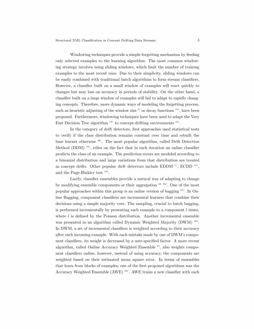
Windowing techniques provide a simple forgetting mechanism by feeding

only selected examples to the learning algorithm. The most common window-

ing strategy involves using sliding windows, which limit the number of training

examples to the most recent ones. Due to their simplicity, sliding windows can

be easily combined with traditional batch algorithms to form stream classifiers.

However, a classifier built on a small window of examples will react quickly to

changes but may lose on accuracy in periods of stability. On the other hand, a

classifier built on a large window of examples will fail to adapt to rapidly chang-

ing concepts. Therefore, more dynamic ways of modeling the forgetting process,

such as heuristic adjusting of the window size 3) or decay functions 10), have been

proposed. Furthermore, windowing techniques have been used to adapt the Very

Fast Decision Tree algorithm 14) to concept-drifting environments 21).

In the category of drift detectors, first approaches used statistical tests

to verify if the class distribution remains constant over time and rebuilt the

base learner otherwise 28). The most popular algorithm, called Drift Detection

Method (DDM) 16), relies on the fact that in each iteration an online classifier

predicts the class of an example. The prediction errors are modeled according to

a binomial distribution and large variations from that distribution are treated

as concept drifts. Other popular dirft detectors include EDDM 1), ECDD 31),

and the Page-Hinkley test 18).

Lastly, classifier ensembles provide a natural way of adapting to change

by modifying ensemble components or their aggregation 23, 24). One of the most

popular approaches within this group is an online version of bagging 27). In On-

line Bagging, component classifiers are incremental learners that combine their

decisions using a simple majority vote. The sampling, crucial to batch bagging,

is performed incrementally by presenting each example to a component l times,

where l is defined by the Poisson distribution. Another incremental ensemble

was presented in an algorithm called Dynamic Weighted Majority (DWM) 22).

In DWM, a set of incremental classifiers is weighted according to their accuracy

after each incoming example. With each mistake made by one of DWM’s compo-

nent classifiers, its weight is decreased by a user-specified factor. A more recent

algorithm, called Online Accuracy Weighted Ensemble 8), also weights compo-

nent classifiers online, however, instead of using accuracy, the components are

weighted based on their estimated mean square error. In terms of ensembles

that learn from blocks of examples, one of the first proposed algorithms was the

Accuracy Weighted Ensemble (AWE) 34). AWE trains a new classifier with each

6 Maciej PIERNIK

incoming block of examples and dynamically weights and rebuilds the ensemble

based on the accuracy of each component. More recently proposed block-based

methods include Learn++NSE 15), which uses a sophisticated accuracy-based

weighting mechanism, and the Accuracy Updated Ensemble (AUE) 9), which

incrementally trains its component classifiers after every processed block of ex-

amples.

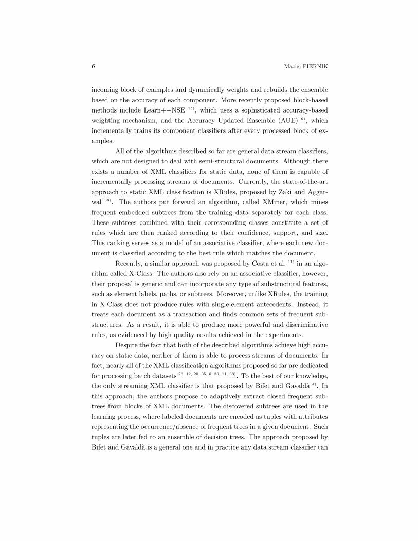
All of the algorithms described so far are general data stream classifiers,

which are not designed to deal with semi-structural documents. Although there

exists a number of XML classifiers for static data, none of them is capable of

incrementally processing streams of documents. Currently, the state-of-the-art

approach to static XML classification is XRules, proposed by Zaki and Aggar-

wal 36). The authors put forward an algorithm, called XMiner, which mines

frequent embedded subtrees from the training data separately for each class.

These subtrees combined with their corresponding classes constitute a set of

rules which are then ranked according to their confidence, support, and size.

This ranking serves as a model of an associative classifier, where each new doc-

ument is classified according to the best rule which matches the document.

Recently, a similar approach was proposed by Costa et al. 11) in an algo-

rithm called X-Class. The authors also rely on an associative classifier, however,

their proposal is generic and can incorporate any type of substructural features,

such as element labels, paths, or subtrees. Moreover, unlike XRules, the training

in X-Class does not produce rules with single-element antecedents. Instead, it

treats each document as a transaction and finds common sets of frequent sub-

structures. As a result, it is able to produce more powerful and discriminative

rules, as evidenced by high quality results achieved in the experiments.

Despite the fact that both of the described algorithms achieve high accu-

racy on static data, neither of them is able to process streams of documents. In

fact, nearly all of the XML classification algorithms proposed so far are dedicated

for processing batch datasets 26, 12, 20, 35, 6, 36, 11, 33). To the best of our knowledge,

the only streaming XML classifier is that proposed by Bifet and Gavalda 4). In

this approach, the authors propose to adaptively extract closed frequent sub-

trees from blocks of XML documents. The discovered subtrees are used in the

learning process, where labeled documents are encoded as tuples with attributes

representing the occurrence/absence of frequent trees in a given document. Such

tuples are later fed to an ensemble of decision trees. The approach proposed by

Bifet and Gavalda is a general one and in practice any data stream classifier can


be used to process documents encoded as tuples. However, such a simple vector

representation may not be sufficient for reacting to several types of drift 7).

§4 The XML Stream ClassifierExisting data stream classification algorithms are not designed to pro-

cess structural data. The algorithm of Bifet and Gavalda 4) transforms XML

documents into vector representations in order to process them using standard

classification algorithms and, therefore, neglects the use of XML-specific similar-

ity measures. Furthermore, the cited approach is capable of dealing with sudden

drifts, but not gradual changes or concept evolution. The aim of our research is

to put forward an XML stream classifier that uses structural similarity measures

and is capable of reacting to different types of drift. To achieve this goal, we

propose to combine associative classification with partial tree-edit distance, in

an algorithm called XML Stream Classifier (XSC).

patterns for

class 1

patterns for

class 2

patterns for

class k

...

prediction

labeled documents

unlabeled documents

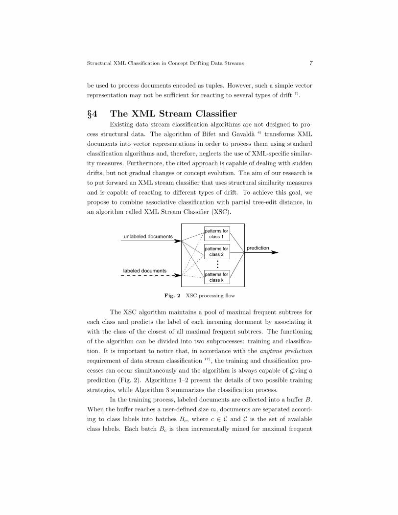
Fig. 2 XSC processing flow

The XSC algorithm maintains a pool of maximal frequent subtrees for

each class and predicts the label of each incoming document by associating it

with the class of the closest of all maximal frequent subtrees. The functioning

of the algorithm can be divided into two subprocesses: training and classifica-

tion. It is important to notice that, in accordance with the anytime prediction

requirement of data stream classification 17), the training and classification pro-

cesses can occur simultaneously and the algorithm is always capable of giving a

prediction (Fig. 2). Algorithms 1–2 present the details of two possible training

strategies, while Algorithm 3 summarizes the classification process.

In the training process, labeled documents are collected into a buffer B.

When the buffer reaches a user-defined size m, documents are separated accord-

ing to class labels into batches Bc, where c ∈ C and C is the set of available

class labels. Each batch Bc is then incrementally mined for maximal frequent

8 Maciej PIERNIK

Algorithm 1 XSC: synchronous training

Input: S: stream of labeled XML documents, m: buffer size, minsup: minimal

support

Output: P: set of patterns for each class (identical patterns from different

classes are considered unique)

1: for all documents dt ∈ S do

2: B ← B ∪ {dt};3: if |B| = m then

4: split documents into batches Bc (c ∈ C) according to class labels;

5: for all c ∈ C: Pc ← AdaTreeNatc(Pc, Bc,minsup);

6: P ←⋃c∈C

Pc;

7: B ← ∅;8: end if

9: end for

Algorithm 2 XSC: asynchronous training

Input: S: stream of labeled XML documents, mc: buffer size for class c,

minsupc: minimal support for class c

Output: P: set of patterns for each class (identical patterns from different

classes are considered unique)


2: c← yt;

3: Bc ← Bc ∪ {dt};4: if |Bc| = mc then

5: Pc ← AdaTreeNatc(Pc, Bc,minsupc);

6: replace set of patterns for c in P with Pc;

7: Bc ← ∅;8: end if

9: end for

subtrees Pc by separate instances of the AdaTreeNat algorithm 4). Since Ada-

TreeNat can mine trees incrementally, existing tree miners for each class are

reused with each new batch of documents. Furthermore, in case of concept-

evolution, a new tree miner can be created without modifying previous models.

After the mining phase, all frequent subtrees are treated as a set of patterns P,

which is used during classification. Each pattern holds the information about


the class it originates from, so identical subtrees from different classes consti-

tute separate, unique patterns. Such patterns, however, are ambiguous in class

assignment. To address this issue, we propose two strategies: i) including these

patterns in the model and weighting them according to their confidence (see

Eq. 2) or ii) removing them entirely from the model. In XSC we use the latter

method, however, the consequences of using either of the proposed approaches

will be evaluated experimentally in Section 5.4. The pseudocode of the described

procedure is presented in Algorithm 1.

The characterized training process updates each class model in a syn-

chronized manner. However, it is worth noticing that if there is class imbalance

in the training data, the classifiers are updated with batches of different sizes.

To address this issue, we propose an alternative, asynchronous update strategy

presented in Algorithm 2. In this strategy the training procedure is slightly al-

tered to achieve a more fluid update procedure. Instead of maintaining a single

buffer B and waiting for m documents to update the model, we create indepen-

dent buffers for each class label. This introduces the possibility of defining a

different batch size for each class and enable better control of the training pro-

cess for class-imbalanced streams. The influence of using either of the presented

strategies will be discussed in Section 5.5.

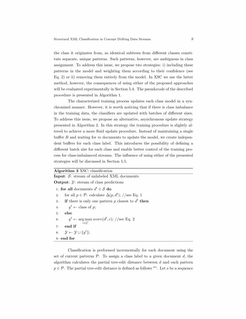
Algorithm 3 XSC: classification

Input: S: stream of unlabeled XML documents

Output: Y: stream of class predictions


2: for all p ∈ P: calculate ∆(p, dt); //see Eq. 1

3: if there is only one pattern p closest to dt then

4: yt ← class of p;

5: else

6: yt ← arg maxc∈C

score(dt, c); //see Eq. 2

7: end if

8: Y ← Y ∪ {yt};9: end for

Classification is performed incrementally for each document using the

set of current patterns P. To assign a class label to a given document d, the

algorithm calculates the partial tree-edit distance between d and each pattern

p ∈ P. The partial tree-edit distance is defined as follows 30). Let s be a sequence

10 Maciej PIERNIK

of tree-edit operations: node relabeling and non-inner node deletion. Both of

these operations have a cost equal to 1. A partial tree-edit sequence s between

two trees p and d is a sequence which transforms p into any subtree of d. The

cost of a partial tree-edit sequence s is the total cost of all operations in s.

Partial tree-edit distance ∆(p, d) between a pattern tree p and a document tree

d is the minimal cost of all possible partial tree-edit sequences between p and d.

∆(p, d) = min {cost(s) : s is a partial tree-edit sequence between p and d} (1)

After using Eq. 1 to calculate distances between d and each pattern

p ∈ P, XSC assigns the class of the pattern closest to d. If there is more than

one closest pattern, we propose a weighted voting measure to decide on the

most appropriate class. In this scenario, each closest pattern p ∈ Pd is granted

a weight based on its confidence in the corresponding class:

confidence(p, c) =|{d ∈ Bc : p ⊆ d}||{d ∈ B : p ⊆ d}|

where Bc are the documents in the last batch with class c and B are all of the

documents in the last batch. This value is then used to vote for the class c

corresponding with the pattern p. The document d is assigned to the class with

the highest score, calculated as follows:

score(d, c) =∑p∈Pd

c

confidence(p, c) (2)

where Pdc are the patterns closest to d with class c.

In contrast to general block-based stream classifiers like AWE 34), AUE 9),

or Learn++NSE 15), the proposed algorithm is designed to work strictly with

structural data. Compared to XML classification algorithms for static data, such

as XRules 36) or X-Class 11), we process documents incrementally, use partial tree-

edit distance, and do not use default rules or rule priority lists. In contrast to the

approach proposed by Bifet and Gavalda 4), XSC does not encode documents into

tuples and calculates pattern-document similarity instead of pattern-document

inclusion. Moreover, since XSC mines for maximal frequent subtrees for each

class separately, it can have different model refresh rates for each class. In case

of class imbalance, independent refresh rates allow the algorithm to mine for

patterns of the minority class using more documents than would be found in

a single batch containing all classes. Additionally, this feature helps to handle

concept-evolution without the need of rebuilding the entire classification model.


Finally, because of its modular nature, the proposed algorithm can be easily im-

plemented in distributed stream environments like Storm∗1, which would enable

high-throughput processing.

§5 Experimental evaluationThe proposed algorithm was evaluated in a series of experiments exam-

ining the impact of different components of XSC and assessing its performance

in scenarios involving different types of drift. In the following subsections, we

describe all of the used datasets, discuss experimental setup, and analyze exper-

iment results.

5.1 DatasetsDuring our experiments we used 4 real and 10 synthetic datasets. The

real datasets were the CSLOG documents, which consist of web logs categorized

into two classes, as described in 36, 4). The first four synthetic datasets were

the DS XML documents generated and analyzed by Zaki and Aggarwal 36). The

additional six synthetic datasets were generated using the tree generation pro-

gram of Zaki, as described in 4). NoDrift contains no drift, Sudden contains 3

sudden drifts every 250k examples, Gradual gradually drifts from the 250k to

750k example, Evolution contains a sudden introduction of a new class after the

1M example. GradualV contains a virtual gradual drift that changes class pro-

portions from 1:1 to 1:10 between the 250k to 750k example. Analogously, the

SuddenV dataset contains 3 sudden drifts that abruptly change class proportions

in the stream from 1:1 to 1:10 and back.

All of the used datasets are summarized in Table 1. As shown in the

table, minimal support and batch size used for tree mining varied depending on

the dataset size and characteristics.

5.2 Experimental setupXSC was implemented in the C# programming language ∗2, tree min-

ing was performed using a C++ implementation of AdaTreeNat 4), while the

remaining classifiers were implemented in Java as part of the MOA framework2). The experiments were conducted on a machine equipped with a dual-core

Intel i7-2640M CPU, 2.8Ghz processor and 16 GB of RAM.

∗1 http://storm-project.net/∗2 Source code, test scripts, and datasets available at:

http://www.cs.put.poznan.pl/dbrzezinski/software.php

12 Maciej PIERNIK

Table 1 Dataset characteristics

Dataset #Examples #Classes #Drifts Drift Minsup Batch

CSLOG12 7628 2 - unknown 1.7% 1000

CSLOG123 15037 2 - unknown 1.7% 1000

CSLOG23 15702 2 - unknown 2.1% 1000

CSLOG31 23111 2 - unknown 2.7% 1500

DS1 91288 2 - unknown 0.8% 5000

DS2 67893 2 - unknown 3.3% 5000

DS3 100000 2 - unknown 0.9% 5000

DS4 75037 2 - unknown 1.3% 5000

NoDrift 1000000 2 0 none 1.0% 10000

Gradual 1000000 2 1 gradual 1.0% 1000

Sudden 1000000 2 3 sudden 1.0% 1000

Evolution 2000000 3 1 mixed 1.0% 10000

GradualV 597456 2 1 gradual 1.0% 1000

SuddenV 644527 2 3 sudden 1.0% 1000

According to the main characteristics of data streams 24, 32), we evaluate

the analyzed algorithms with respect to time efficiency, memory usage, and

predictive performance. All the evaluation measures were calculated using the

block evaluation method, which works similarly to the test-then-train paradigm

with the difference that it uses data blocks instead of single examples. This

method reads incoming examples without processing them, until they form a

data block of size b. Each new data chunk is first used to evaluate the existing

classifier, then it updates the classifier, and finally it is disposed to preserve

memory. Such an approach allows to measure average block training and testing

times and is less pessimistic than the test-then-train method.

To assess the predictive power of the analyzed algorithms we used the

accuracy measure, defined as follows:

accuracy =

∑c∈C

(|Dtest

c ||Dc|

)|C|

where C is the set of all classes, Dc are the documents with class c, and Dtestc

are the documents correctly assigned to class c by the classifier. This model

for calculating accuracy is often referred to as equal, as it calculates an equally

weighted average of all class-wise accuracies. As a result, the performance mea-


sure is unaffected by class imbalance in the dataset and for a random classifier

is on average equal to 50%. We decided to use this model because nearly all of

our datasets are to some extent imbalanced.

Additionally, we used statistical tests to verify the significance of our

findings. To compare multiple algorithms on multiple datasets we used the

Iman and Davenport variation of the Friedman test combined with the Nemenyi

post-hoc test 13). According to the test procedure, for each dataset each algo-

rithm was granted a score from 1 to k based on its performance, where k is the

number of compared algorithms and lower ranks signify better results. Based

on these rankings, average ranks for all algorithms were calculated and used to

compute the Friedman statistic. The null-hypothesis for this test is that there

is no difference between the performance of all of the tested algorithms. In case

of rejecting this null-hypothesis, the post-hoc Nemenyi test was conducted to

calculate the critical distance indicating significant differences between pairs of

approaches.

Finally, when only two algorithms were compared on multiple datasets,

we used the Wilcoxon signed-rank test 13). In such cases, the differences in

performance between the algorithms on each dataset were calculated and ranked

according to their absolute values from 1 to the number of datasets, 1 being

the lowest rank. The ranks were then summed separately for positive R+ and

negative R− differences and the lower sum was tested against the critical value.

Rejecting the null-hypothesis indicates that one algorithm preforms significantly

better than the other.

5.3 Vote weightingThe goal of the first experiment was to check how various weighting

schemes influence the accuracy of our algorithm. In XSC, weighting is used only

when several patterns are found in the same, closest proximity to the document

being classified. Apart from confidence, described in Section 4, we have also

considered three additional weighting functions:

• size — number of nodes in the pattern tree,

• support — frequency of a pattern p in the last batch of documents Bc

with the same class as p:

support(p, c) =|d ∈ Bc : p ⊆ d|

|Bc|

• equal — each pattern assigned an equal weight of 1.

14 Maciej PIERNIK

All four weighting functions were tested on all datasets. As weighting can resolve

the ambiguity of duplicate patterns (the same patterns occurring in several class

models), in this test, we did not remove such patterns from the model. The

result of this experiment is presented in Table 2. The last row represents the

average ranks of the algorithms used for the Friedman test.

Table 2 Comparison of pattern weighting schemes

Dataset Equal Size Support Confidence

DS1 67.38% 67.66% 63.95% 67.88%

DS2 67.80% 69.26% 53.11% 69.25%

DS3 59.89% 60.50% 57.74% 58.24%

DS4 58.51% 58.31% 58.46% 58.50%

CSLOG12 57.93% 59.78% 58.26% 59.65%

CSLOG23 59.72% 61.28% 59.51% 60.81%

CSLOG31 59.00% 60.59% 59.24% 60.40%

CSLOG123 58.48% 60.32% 57.36% 61.88%

NoDrift 99.99% 99.99% 99.99% 99.99%

Gradual 97.78% 97.73% 97.65% 97.80%

Sudden 99.35% 99.34% 99.30% 99.36%

Evolution 99.33% 99.33% 99.33% 99.33%

GradualV 99.88% 99.81% 99.88% 99.75%

SuddenV 99.66% 99.66% 99.66% 99.66%

Rank 2.571 2.107 3.286 2.036

As the results show, confidence and size perform best, whereas weighting

with support produced the worst results on most of the datasets. Analyzing the

results vertically, one can observe that the DS and CSLOG datasets are much

more affected by the changes in the weighting strategy than the drift datasets.

In order to determine whether the proposed weighting strategies signifi-

cantly influence the quality of our approach, we performed a Friedman test. The

FF score for this experiment equals 6.426, so with α = 0.05 and FCritical = 2.850,

we can reject the null-hypothesis that the differences in the results are random.

However, the additional Nemenyi test does not favor any weighting function over

the other. With confidence performing slightly better than size, we decided to

weight indistinguishably similar patterns according to their confidence.


5.4 Duplicate pattern treatmentThe aim of this experiment was to compare the two strategies for han-

dling duplicate patterns discussed in Section 4. The first one involved including

such patterns in the classification model and weighting them according to their

confidence while in the second strategy such patterns were removed. The re-

sult of this experiment is given in Table 3. The two last columns represent the

difference in accuracy and a rank required by the Wilcoxon signed-rank test.

Table 3 Duplicate pattern treatment

Dataset Left Removed Diff Rank

DS1 67.88% 68.12% -0.24% 6

DS2 69.25% 69.25% 0.00% n/a

DS3 58.24% 58.55% -0.31% 7

DS4 58.50% 58.51% -0.01% 1.5

CSLOG12 59.65% 59.64% 0.01% 1.5

CSLOG23 60.81% 61.30% -0.50% 8

CSLOG31 60.40% 60.34% 0.06% 4

CSLOG123 61.88% 60.94% 0.93% 9

NoDrift 99.99% 99.99% 0.00% n/a

Gradual 97.80% 97.66% 0.14% 5

Sudden 99.36% 99.41% -0.05% 3

Evolution 99.33% 99.33% 0.00% n/a

GradualV 99.75% 99.75% 0.00% n/a

SuddenV 99.66% 99.66% 0.00% n/a

The results of this experiment are inconclusive. The differences between

both of these approaches are very small for all datasets. Moreover, both methods

achieve the best result for nearly the same number of datasets. To make sure that

the result carries no statistical significance, we performed a Wilcoxon signed-rank

test. At α = 0.05 we were unable to reject the null-hypothesis (W = 19.5 >

Wcrit = 9), thus the experiment data is insufficient to indicate any significant

difference between these approaches. Given the above, in XSC we chose to

remove duplicate patterns in order to make a more compact model.

5.5 Synchronized updateIn Section 4 we proposed two approaches to training a classifier: asyn-

chronous — where each class model is updated whenever its own document buffer

16 Maciej PIERNIK

is full (Algorithm 2) and synchronous — in which updates are carried out only

when the global buffer is full (Algorithm 1). In this experiment, we compared

the synchronous and asynchronous strategies. The results of this comparison

are presented in Table 4. As in the previous test, the two last columns represent

the difference in quality and a rank of that difference, respectively.

Table 4 Comparison of asynchronous and synchronous updating of classification models.

Dataset Asynchronous Synchronous Diff Rank

DS1 67.88% 63.22% 4.66% 11

DS2 69.25% 63.95% 5.3% 12

DS3 58.24% 56.08% 2.16% 5

DS4 58.50% 50.62% 7.88% 14

CSLOG12 59.65% 59.88% -0.23% 1

CSLOG23 60.81% 56.68% 4.13% 10

CSLOG31 60.40% 53.91% 6.49% 13

CSLOG123 61.88% 59.59% 2.29% 6

NoDrift 99.99% 96.00% 3.99% 9

Gradual 97.80% 95.48% 2.32% 7

Sudden 99.36% 97.22% 2.14% 4

Evolution 99.33% 96.56% 2.77% 8

GradualV 99.75% 98.16% 1.59% 2

SuddenV 99.66% 97.63% 2.03% 3

The obtained results clearly indicate that the asynchronous model is

superior to the synchronous one, as it performs better on 13 out of 14 datasets.

This result is confirmed by a one-tailed Wilcoxon signed-rank test with p =

0.0006, therefore, we can reject the null-hypothesis that both approaches are

equivalent and state that updating models asynchronously works significantly

better than synchronous updates.

There are two factors which contribute to this outcome. Firstly, in the

asynchronous model there are as many buffers as there are classes, so the size of

the global buffer is actually |C| times the size of each class buffer. As a result,

when there is more than one class, the asynchronous model is updated with

larger batches. Secondly, in the synchronous model there is no guarantee that

the class batches are of equal size. Since the global buffer is split on overflow,

if there is class imbalance in the dataset it will be reflected in the sizes of class

batches. The asynchronous model is immune to this problem.


5.6 Comparative analysisThe aim of the final set of experiments was to compare XSC with

eight streaming classifiers employing the methodology proposed by Bifet and

Gavalda 4): Online Bagging (Bag) 27), Online Accuracy Updated Ensemble

(OAUE) 8), Dynamic Weighted Majority (DWM), Learn++.NSE (NSE) 15), Ac-

curacy Weighted Ensemble (AWE) 34), Accuracy Updated Ensemble (AUE) 9),

Drift Detection Method with a Hoeffding Tree (DDM), and the Naive Bayes al-

gorithm (NB). Bagging was chosen as the algorithm used by Bifet and Gavalda

to test their methodology, while OAUE and DWM were selected as alternative

online ensembles. We chose DDM as a representative of drift detectors and Naive

Bayes as an example of a method without any drift reaction mechanisms. The

remaining algorithms (AWE, AUE, NSE) were chosen as strong representatives

of block-based stream classifiers.

To make the comparison more meaningful, we set the same parameter

values for all the algorithms. For ensemble methods we set the number of com-

ponent classifiers to 10: AUE, NSE, DWM, Bag, and OAUE have ten Hoeffding

Trees, and since AWE uses static learners it has ten J48 trees. We decided to

use 10 component classifiers as this was the number suggested and tested in 4).

The data block size used for block-based classifiers (AWE, AUE, NSE) was the

same as the maximal frequent subtree mining batch size (see Section 5.1). For

ensemble components we used Hoeffding Trees enhanced with Naive Bayes leaf

predictions with a grace period nmin = 100, split confidence δ = 0.01, and

tie-threshold τ = 0.05 14).

All of the analyzed algorithms were tested in terms of accuracy, clas-

sification time, and memory usage. The results were obtained using the block

evaluation procedure, with pattern mining (model updates) occurring after each

block of examples. Tables 5–7 present accuracy, average block classification time,

and average memory usage, obtained by the tested algorithms on all datasets,

respectively.

Apart from analyzing the average performance of algorithms, we gen-

erated graphical plots for each dataset depicting the algorithms’ functioning in

terms of classification accuracy. By presenting the performance measure calcu-

lated after each data chunk on the y-axis and the number of processed training

examples on the x-axis, one can examine the dynamics of a given classifier, in

particular, its reactions to concept drift. Such graphical plots are the most

common way of displaying results in data stream mining papers 15, 5). We will

18 Maciej PIERNIK

Table

5C

om

pari

son

of

vari

ou

sst

ream

class

ifier

s—

over

all

acc

ura

cy[%

].

Dat

aset

AU

EA

WE

Bag

DW

MD

DM

NS

EN

BO

AU

EX

SC

DS

162

.61

61.

6163.0

361.5

662.2

058.8

162.9

462.6

267.88

DS

270

.02

69.5

871.03

68.1

170.0

667.7

865.4

170.0

269.2

4

DS

358

.51

58.4

658.53

58.3

958.5

055.2

057.1

658.5

158.2

4

DS

460

.83

60.4

461.42

59.8

460.7

258.3

560.5

960.8

358.5

0

CS

LO

G12

53.6

955

.38

53.0

451.7

350.3

050.0

054.9

853.6

959.64

CS

LO

G23

53.2

953

.57

52.9

652.0

653.0

351.5

954.0

153.2

560.80

CS

LO

G31

51.8

652

.06

52.1

351.3

751.7

550.6

552.0

752.3

660.40

CS

LO

G12

352

.95

52.

9654.6

154.7

054.0

851.3

255.0

353.1

261.87

NoD

rift

53.7

754

.00

53.7

353.7

553.6

952.0

454.1

953.8

799.99

Su

dd

en53

.24

52.

8752.9

353.1

852.9

053.0

449.9

953.2

399.35

Su

dd

enV

62.9

161.

4962.8

062.8

861.8

262.1

559.5

262.9

099.65

Gra

du

al53

.19

52.

8252.8

853.1

052.8

952.8

251.4

253.1

897.80

Gra

du

alV

55.4

253.

5655.4

455.4

355.4

351.5

955.4

655.3

899.74

Evo

luti

on57

.80

61.

5859.0

357.8

158.0

558.4

353.3

357.2

999.32

Ran

k4.

250

5.4

293.9

29

5.8

57

5.6

43

8.0

00

5.4

29

4.1

79

2.286


Table

6C

om

pari

son

of

vari

ou

sst

ream

class

ifier

s—

aver

age

batc

hp

roce

ssin

gti

me

[s].

Dat

aset

AU

EA

WE

Bag

DW

MD

DM

NS

EN

BO

AU

EX

SC

DS

11.

184

1.1

371.2

25

1.1

41

1.1

06

1.105

1.1

08

1.1

89

1.0

65

DS

20.

326

0.3

140.3

48

0.3

05

0.300

0.3

03

0.3

08

0.3

26

2.3

65

DS

31.

142

1.10

81.1

90

1.1

43

1.0

78

1.072

1.0

74

1.1

66

1.0

92

DS

40.

549

0.5

290.5

92

0.5

27

0.506

0.5

09

0.5

10

0.5

50

0.7

76

CS

LO

G12

1.09

81.

093

1.1

01

1.1

09

1.088

1.0

93

1.0

93

1.0

93

2.0

58

CS

LO

G23

1.06

71.

056

1.0

82

1.0

67

1.0

61

1.0

56

1.0

63

1.0

65

0.741

CS

LO

G31

0.38

70.3

810.3

88

0.3

85

0.379

0.379

0.3

81

0.3

86

1.7

53

CS

LO

G12

31.

433

1.41

91.4

44

1.4

28

1.4

19

1.4

20

1.4

30

1.4

32

1.110

NoD

rift

0.79

30.6

851.2

70

1.2

08

0.7

03

0.6

74

0.662

0.8

71

1.4

81

Su

dd

en0.

077

0.0

690.1

71

0.0

92

0.0

73

0.0

72

0.068

0.0

76

0.0

97

Su

dd

enV

0.07

80.066

0.1

11

0.2

13

0.0

69

0.0

69

0.066

0.0

76

0.1

01

Gra

du

al0.

075

0.06

90.1

70

0.0

87

0.0

70

0.0

72

0.068

0.0

76

1.1

30

Gra

du

alV

0.07

40.062

0.1

06

0.7

96

0.0

65

0.0

63

0.062

0.0

71

0.1

00

Evo

luti

on0.

243

0.09

81.3

18

0.9

91

0.1

66

0.1

02

0.079

0.2

66

0.1

00

Ran

k6.

286

3.1

438.3

57

6.6

07

2.8

93

2.714

2.714

6.1

43

6.1

43

20 Maciej PIERNIK

Table

7C

om

pari

son

of

vari

ou

sst

ream

class

ifier

s—

aver

age

batc

hm

od

elm

emory

[kB

].

Dat

aset

AU

EA

WE

Bag

DW

MD

DM

NS

EN

BO

AU

EX

SC

DS

140

00.2

9325

946.

680

616

0.5

47

1844.6

19

521.9

11

334.5

39

47.3

62

4408.4

67

8.936

DS

263

0.79

674

89.6

29105

4.1

99

125.5

21

97.8

83

213.3

29

11.6

86

969.0

22

10.391

DS

331

92.5

8820

836.

523

4899

.053

3036.0

35

445.5

42

197.7

14

36.0

56

3662.0

61

8.242

DS

499

1.06

410

899.

316

1526

.865

460.7

29

144.1

82

142.2

99

18.1

18

1360.6

05

6.816

CS

LO

G12

818.

133

8553

.180

243

3.2

13

867.2

86

124.2

98

110.0

66

124.5

58

871.0

66

6.680

CS

LO

G23

5135

.010

2594

3.89

110

129.0

04

1807.1

88

832.9

90

218.2

48

253.1

87

5323.5

06

3.672

CS

LO

G31

1520

.020

8235

.176

329

9.3

36

1556.7

85

198.1

97

77.0

44

75.7

05

1773.6

52

6.064

CS

LO

G12

370

67.9

5934

427.

637

131

99.0

23

3503.2

62

1354.3

85

590.1

48

230.3

32

7823.1

35

4.941

NoD

rift

265.

082

1434

3.84

8734

.486

640.2

69

57.0

31

380.2

83

7.3

73

1195.5

47

3.037

Su

dd

en32

7.54

328

22.3

44

1289

.326

776.1

14

114.3

71

12654.3

95

14.6

48

412.8

46

2.676

Su

dd

enV

418.

344

3168

.096

1013

.506

2332.4

51

84.6

51

6242.9

49

17.1

08

487.6

06

2.686

Gra

du

al31

2.63

427

30.5

96

1209

.395

631.9

71

80.8

58

12641.4

06

13.9

32

414.9

04

2.764

Gra

du

alV

399.

175

2800

.234

843

.497

4791.6

50

72.1

22

4461.5

82

14.2

62

445.9

99

2.676

Evo

luti

on36

9.64

821

401.

465

136

1.9

34

1062.8

61

110.9

59

1234.8

73

13.4

54

1274.6

58

2.676

Ran

k5.

000

8.643

7.5

00

5.7

14

3.4

29

5.0

00

2.2

14

6.5

00

1.000


analyze the most interesting plots, which highlight characteristic features of the

studied algorithms.

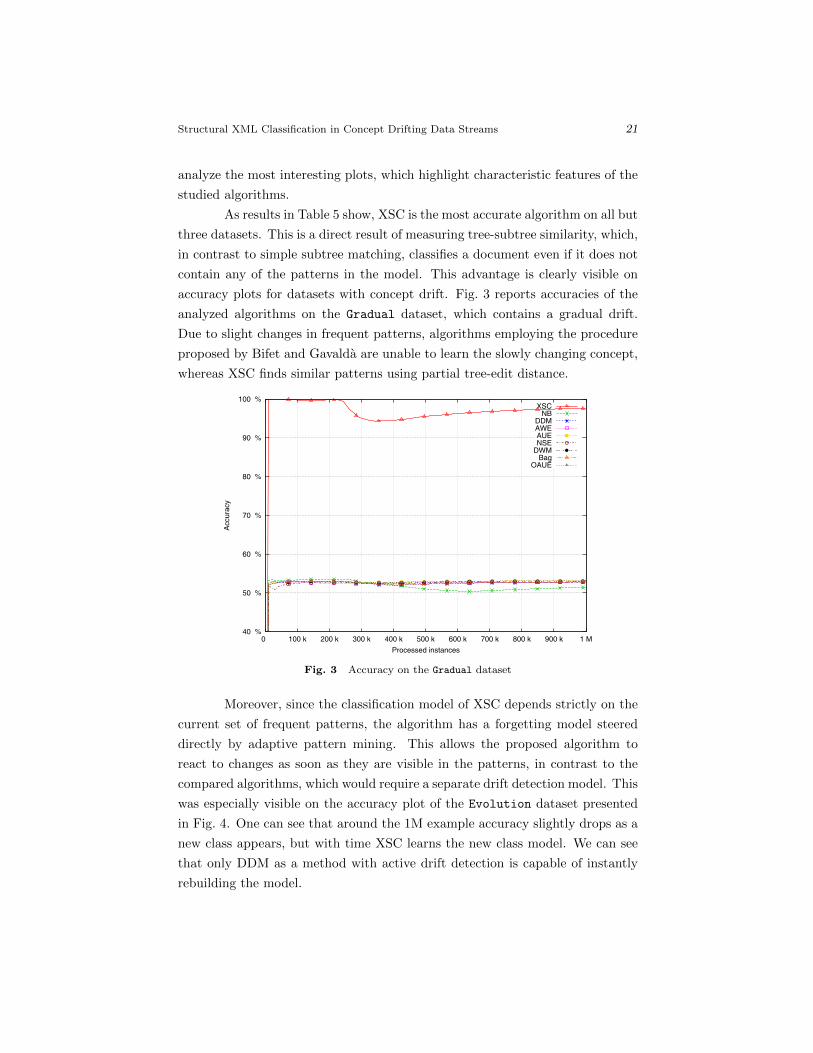
As results in Table 5 show, XSC is the most accurate algorithm on all but

three datasets. This is a direct result of measuring tree-subtree similarity, which,

in contrast to simple subtree matching, classifies a document even if it does not

contain any of the patterns in the model. This advantage is clearly visible on

accuracy plots for datasets with concept drift. Fig. 3 reports accuracies of the

analyzed algorithms on the Gradual dataset, which contains a gradual drift.

Due to slight changes in frequent patterns, algorithms employing the procedure

proposed by Bifet and Gavalda are unable to learn the slowly changing concept,

whereas XSC finds similar patterns using partial tree-edit distance.

40 %

50 %

60 %

70 %

80 %

90 %

100 %

0 100 k 200 k 300 k 400 k 500 k 600 k 700 k 800 k 900 k 1 M

Accura

cy

Processed instances

XSCNB

DDMAWEAUENSE

DWMBag

OAUE

Fig. 3 Accuracy on the Gradual dataset

Moreover, since the classification model of XSC depends strictly on the

current set of frequent patterns, the algorithm has a forgetting model steered

directly by adaptive pattern mining. This allows the proposed algorithm to

react to changes as soon as they are visible in the patterns, in contrast to the

compared algorithms, which would require a separate drift detection model. This

was especially visible on the accuracy plot of the Evolution dataset presented

in Fig. 4. One can see that around the 1M example accuracy slightly drops as a

new class appears, but with time XSC learns the new class model. We can see

that only DDM as a method with active drift detection is capable of instantly

rebuilding the model.

22 Maciej PIERNIK

40 %

50 %

60 %

70 %

80 %

90 %

100 %

200 k 400 k 600 k 800 k 1 M 1 M 1 M 2 M 2 M 2 M

Accura

cy

Processed instances

XSCNB

DDMAWEAUENSE

DWMBag

OAUE

Fig. 4 Accuracy on the Evolution dataset

40 %

50 %

60 %

70 %

80 %

90 %

100 %

0 100 k 200 k 300 k 400 k 500 k 600 k

Accura

cy

Processed instances

XSCNB

DDMAWEAUENSE

DWMBag

OAUE

Fig. 5 Accuracy on the SuddenV dataset


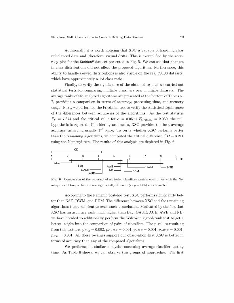
Additionally it is worth noticing that XSC is capable of handling class

imbalanced data and, therefore, virtual drifts. This is exemplified by the accu-

racy plot for the SuddenV dataset presented in Fig. 5. We can see that changes

in class distributions did not affect the proposed algorithm. Furthermore, this

ability to handle skewed distributions is also visible on the real CSLOG datasets,

which have approximately a 1:3 class ratio.

Finally, to verify the significance of the obtained results, we carried out

statistical tests for comparing multiple classifiers over multiple datasets. The

average ranks of the analyzed algorithms are presented at the bottom of Tables 5–

7, providing a comparison in terms of accuracy, processing time, and memory

usage. First, we performed the Friedman test to verify the statistical significance

of the differences between accuracies of the algorithms. As the test statistic

FF = 7.374 and the critical value for α = 0.05 is FCritical = 2.030, the null

hypothesis is rejected. Considering accuracies, XSC provides the best average

accuracy, achieving usually 1st place. To verify whether XSC performs better

than the remaining algorithms, we computed the critical difference CD = 3.211

using the Nemenyi test. The results of this analysis are depicted in Fig. 6.

2 3 4

CD

XSC

1 5 6 7 8 9

Bag

OAUE

AUE

AWE

NB DDM

DWM NSE

Fig. 6 Comparison of the accuracy of all tested classifiers against each other with the Ne-

menyi test. Groups that are not significantly different (at p = 0.05) are connected.

According to the Nemenyi post-hoc test, XSC performs significantly bet-

ter than NSE, DWM, and DDM. The difference between XSC and the remaining

algorithms is not sufficient to reach such a conclusion. Motivated by the fact that

XSC has an accuracy rank much higher than Bag, OAUE, AUE, AWE and NB,

we have decided to additionally perform the Wilcoxon signed-rank test to get a

better insight into the comparison of pairs of classifiers. The p-values resulting

from this test are: pBag = 0.002, pOAUE = 0.001, pAUE = 0.001, pAWE = 0.001,

pNB = 0.001. All these p-values support our observation that XSC is better in

terms of accuracy than any of the compared algorithms.

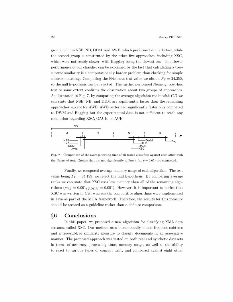
We performed a similar analysis concerning average classifier testing

time. As Table 6 shows, we can observe two groups of approaches. The first

24 Maciej PIERNIK

group includes NSE, NB, DDM, and AWE, which performed similarly fast, while

the second group is constituted by the other five approaches, including XSC,

which were noticeably slower, with Bagging being the slowest one. The slower

performance of our classifier can be explained by the fact that calculating a tree-

subtree similarity is a computationally harder problem than checking for simple

subtree matching. Computing the Friedman test value we obtain FF = 24.250,

so the null hypothesis can be rejected. The further performed Nemenyi post-hoc

test to some extent confirms the observation about two groups of approaches.

As illustrated in Fig. 7, by comparing the average algorithm ranks with CD we

can state that NSE, NB, and DDM are significantly faster than the remaining

approaches, except for AWE. AWE performed significantly faster only compared

to DWM and Bagging but the experimental data is not sufficient to reach any

conclusion regarding XSC, OAUE, or AUE.

2 3 4

CD

XSC

1 5 6 7 8 9

Bag

OAUEAUE

AWE

NBDDM

DWMNSE

Fig. 7 Comparison of the average testing time of all tested classifiers against each other with

the Nemenyi test. Groups that are not significantly different (at p = 0.05) are connected.

Finally, we compared average memory usage of each algorithm. The test

value being FF = 84.199, we reject the null hypothesis. By comparing average

ranks we can state that XSC uses less memory than all of the remaining algo-

rithms (pNB = 0.001, pDDM = 0.001). However, it is important to notice that

XSC was written in C#, whereas the competitive algorithms were implemented

in Java as part of the MOA framework. Therefore, the results for this measure

should be treated as a guideline rather than a definite comparison.

§6 ConclusionsIn this paper, we proposed a new algorithm for classifying XML data

streams, called XSC. Our method uses incrementally mined frequent subtrees

and a tree-subtree similarity measure to classify documents in an associative

manner. The proposed approach was tested on both real and synthetic datasets

in terms of accuracy, processing time, memory usage, as well as the ability

to react to various types of concept drift, and compared against eight other


XML data stream classifiers. Furthermore, we experimentally evaluated various

components of our algorithm, namely: dealing with duplicate patterns occurring

in more than one class; weighting votes during class assignment when more than

one pattern was found in the same distance to the document being classified;

synchronizing the updates of classifier models.

The comparative analysis shows that XSC performs significantly better

than all of its competitors in terms of accuracy and memory usage. Further-

more, it was able to efficiently adapt to various changes in the data introduced

by several types of concept drift. The analysis of different strategies concern-

ing duplicate pattern treatment and vote weighting did not significantly favor

any approach over another, however, resolving ambiguities with confidence gave

the best results on average. Since no difference in accuracy was found between

including and removing the duplicate patterns, we can safely exclude such pat-

terns from the model to improve the processing time and memory usage. Finally,

synchronizing the updates of all classifiers proved to be significantly worse than

updating each model asynchronously.

The high predictive power of our approach comes at a cost of longer clas-

sification time. XSC was shown to be significantly slower than three competing

approaches, although on average performed equally fast or faster than four of

the remaining algorithms. This is due to using partial tree-edit distance, a com-

plex tree-subtree similarity measure which requires more processing time than

simple subtree matching used in the competing algorithms. This issue could be

addressed in the future by proposing a heuristic method for assessing the tree-

subtree similarity. Moreover, an algorithm capable of working in distributed

environments could also be investigated.

Acknowledgment D. Brzezinski’s and M. Piernik’s research is funded

by the Polish National Science Center under Grants No. DEC-2011/03/N/ST6/

00360 and DEC-2011/01/B/ST6/05169, respectively.

References

1) M. Baena-Garcıa, J. del Campo-Avila, R. Fidalgo, A. Bifet, R. Gavalda, andR. Morales-Bueno, “Early drift detection method,” in In Fourth InternationalWorkshop on Knowledge Discovery from Data Streams, 2006.

2) A. Bifet et al., “MOA: Massive Online Analysis,” J. Mach. Learn. Res., vol. 11,pp. 1601–1604, 2010.

3) A. Bifet and R. Gavalda, “Learning from time-changing data with adaptive

26 Maciej PIERNIK

windowing,” in SDM, D. Skillicorn, B. Liu, C. Apte, and S. Parthasarathy, Eds.SIAM, 2007.

4) A. Bifet and R. Gavalda, “Adaptive xml tree classification on evolving datastreams,” in Proc. ECML/PKDD 2009 (1). LNCS Vol. 5781, 2009, pp. 147–162.

5) A. Bifet, G. Holmes, and B. Pfahringer, “Leveraging bagging for evolving datastreams,” in ECML/PKDD (1), 2010, pp. 135–150.

6) A. Bouchachia and M. Hassler, “Classification of XML Documents,” in CIDM2007 Proceedings, 2007, pp. 390–396.

7) D. Brzezinski and M. Piernik, “Adaptive XML stream classification using partialtree-edit distance,” in Foundations of Intelligent Systems - 21st InternationalSymposium, ISMIS 2014, Roskilde, Denmark, June 25-27, 2014. Proceedings,ser. Lecture Notes in Computer Science, T. Andreasen, H. Christiansen,J. C. C. Talavera, and Z. W. Ras, Eds., vol. 8502. Springer, 2014, pp. 10–19.[Online]. Available: http://dx.doi.org/10.1007/978-3-319-08326-1 2

8) D. Brzezinski and J. Stefanowski, “Combining block-based and online methodsin learning ensembles from concept drifting data streams,” Information Sciences,vol. 265, pp. 50–67, 2014.

9) ——, “Reacting to different types of concept drift: The accuracy updated en-semble algorithm,” IEEE Trans. on Neural Netw. Learn. Syst., vol. 25, no. 1,pp. 81–94, 2014.

10) E. Cohen and M. J. Strauss, “Maintaining time-decaying stream aggregates,”J. Algorithms, vol. 59, no. 1, pp. 19–36, 2006.

11) G. Costa, R. Ortale, and E. Ritacco, “X-class: Associative classification ofXML documents by structure,” ACM Trans. Inf. Syst., vol. 31, no. 1, p. 3,2013. [Online]. Available: http://doi.acm.org/10.1145/2414782.2414785

12) C. M. De Vries et al., “Overview of the inex 2010 xml mining track : clusteringand classification of xml documents,” in Initiative for the Evaluation of XMLRetrieval (INEX) 2010, 2011.

13) J. Demsar, “Statistical comparisons of classifiers over multiple data sets,” J.Machine Learning Research, vol. 7, pp. 1–30, 2006.

14) P. Domingos and G. Hulten, “Mining high-speed data streams,” in Proc. 6thACM SIGKDD Int. Conf. Knowl. Disc. Data Min., 2000, pp. 71–80.

15) R. Elwell and R. Polikar, “Incremental learning of concept drift in nonstationaryenvironments,” IEEE Trans. Neural Netw., vol. 22, no. 10, pp. 1517–1531, 2011.

16) J. Gama, P. Medas, G. Castillo, and P. Rodrigues, “Learning with drift detec-tion,” in Proc. 17th SBIA Brazilian Symp. Art. Intel., 2004, pp. 286–295.

17) J. Gama, Knowledge Discovery from Data Streams. Chapman and Hall, 2010.

18) J. Gama, R. Sebastiao, and P. P. Rodrigues, “On evaluating stream learningalgorithms,” Machine Learning, vol. 90, no. 3, pp. 317–346, 2013.

19) J. Gama, I. Zliobaite, A. Bifet, M. Pechenizkiy, and A. Bouchachia, “A surveyon concept drift adaptation,” ACM Computing Surveys, vol. 46, no. 4, 2014.

20) C. Garboni et al., “Sequential Pattern Mining for Structure-based XML Docu-ment Classification,” in INEX 2005 Proceedings, 2006, pp. 458–468.

21) G. Hulten, L. Spencer, and P. Domingos, “Mining time-changing data streams,”in KDD, 2001, pp. 97–106.


22) J. Z. Kolter and M. A. Maloof, “Dynamic weighted majority: An ensemblemethod for drifting concepts,” J. Mach. Learn. Res., vol. 8, pp. 2755–2790,2007.

23) L. I. Kuncheva, “Classifier ensembles for changing environments,” in Proc. 5thMCS Int. Workshop on Mult. Class. Syst., ser. LNCS, vol. 3077. Springer,2004, pp. 1–15.

24) ——, “Classifier ensembles for detecting concept change in streaming data:Overview and perspectives,” in 2nd Workshop SUEMA 2008 (ECAI 2008),2008, pp. 5–10.

25) V. Mayorga and N. Polyzotis, “Sketch-based summarization of ordered XMLstreams,” in ICDE, Y. E. Ioannidis, D. L. Lee, and R. T. Ng, Eds. IEEE, 2009,pp. 541–552.

26) R. Nayak et al., “Overview of the INEX 2009 XML Mining Track: Clusteringand Classification of XML Documents,” in Focused Retrieval and Evaluation,vol. 6203, 2010, pp. 366–378.

27) N. C. Oza and S. J. Russell, “Experimental comparisons of online and batch ver-sions of bagging and boosting,” in Proc. 7th ACM SIGKDD Int. Conf. Knowl.Disc. Data Min., 2001, pp. 359–364.

28) E. S. Page, “Continuous inspection schemes,” Biometrika, vol. 41, no. 1/2, pp.100–115, 1954. [Online]. Available: http://dx.doi.org/10.2307/2333009

29) M. Piernik, D. Brzezinski, T. Morzy, and A. Lesniewska, “XML clustering:A review of structural approaches,” The Knowledge Engineering Review, vol.30(03), pp. 297–323, 2015.

30) M. Piernik and T. Morzy, “Partial tree-edit distance,” Poznan University ofTechnology, Tech. Rep. RA-10/2013, 2013, available at:http://www.cs.put.poznan.pl/mpiernik/publications/PTED.pdf.

31) G. J. Ross, N. M. Adams, D. K. Tasoulis, and D. J. Hand, “Exponentiallyweighted moving average charts for detecting concept drift,” Pattern RecognitionLetters, vol. 33, no. 2, pp. 191–198, 2012.

32) W. N. Street and Y. Kim, “A streaming ensemble algorithm (SEA) for large-scale classification,” in Proc. 7th ACM SIGKDD Int. Conf. Knowl. Disc. DataMin. New York, NY, USA: ACM Press, 2001, pp. 377–382.

33) N. Thasleena and S. Varghese, “Enhanced associative classification of XML doc-uments supported by semantic concepts,” Procedia Computer Science, vol. 46,pp. 194–201, 2015.

34) H. Wang et al., “Mining concept-drifting data streams using ensemble classi-fiers,” in Proc. 9th ACM SIGKDD Int. Conf. Knowl. Disc. Data Min., 2003,pp. 226–235.

35) J. Yang and S. Wang, “Extended VSM for XML Document Classification UsingFrequent Subtrees,” in INEX 2009 Proceedings, 2010, pp. 441–448.

36) M. J. Zaki and C. C. Aggarwal, “XRules: An effective algorithm for structuralclassification of xml data,” Machine Learning, vol. 62, no. 1-2, pp. 137–170,2006.

Structural XML Classi cation in Concept Drifting Data Streams · Structural XML Classi cation in...

Documents

Transcript of Structural XML Classi cation in Concept Drifting Data Streams · Structural XML Classi cation in...