Structural Matrices in MDOF Systems - GitHub Pages · Structural Matrices Giacomo Boffi...
75
Structural Matrices Giacomo Boffi Introductory Remarks Structural Matrices Evaluation of Structural Matrices Choice of Property Formulation Structural Matrices in MDOF Systems Giacomo Boffi http://intranet.dica.polimi.it/people/boffi-giacomo Dipartimento di Ingegneria Civile Ambientale e Territoriale Politecnico di Milano April 8, 2016
-
Upload
nguyenkhanh -
Category
Documents
-
view
223 -
download
0
Transcript of Structural Matrices in MDOF Systems - GitHub Pages · Structural Matrices Giacomo Boffi...

StructuralMatrices
Giacomo Boffi
IntroductoryRemarks
StructuralMatrices
Evaluation ofStructuralMatrices
Choice ofPropertyFormulation
Structural Matrices in MDOF Systems
Giacomo Boffi
http://intranet.dica.polimi.it/people/boffi-giacomo
Dipartimento di Ingegneria Civile Ambientale e TerritorialePolitecnico di Milano
April 8, 2016
StructuralMatrices
Giacomo Boffi
IntroductoryRemarks
StructuralMatrices
Evaluation ofStructuralMatrices
Choice ofPropertyFormulation
Outline
Introductory RemarksStructural Matrices
Orthogonality RelationshipsAdditional Orthogonality Relationships
Evaluation of Structural MatricesFlexibility MatrixExampleStiffness MatrixMass MatrixDamping MatrixGeometric StiffnessExternal Loading
Choice of Property FormulationStatic CondensationExample

StructuralMatrices
Giacomo Boffi
IntroductoryRemarks
StructuralMatrices
Evaluation ofStructuralMatrices
Choice ofPropertyFormulation
Introductory Remarks
Today we will study the properties of structural matrices, that is theoperators that relate the vector of system coordinates x and its timederivatives x and x to the forces acting on the system nodes, fS, fDand fI, respectively.
In the end, we will see again the solution of a MDOF problem bysuperposition, and in general today we will revisit many of thesubjects of our previous class, but you know that a bit of reiterationis really good for developing minds.

StructuralMatrices
Giacomo Boffi
IntroductoryRemarks
StructuralMatrices
Evaluation ofStructuralMatrices
Choice ofPropertyFormulation
Introductory Remarks
Today we will study the properties of structural matrices, that is theoperators that relate the vector of system coordinates x and its timederivatives x and x to the forces acting on the system nodes, fS, fDand fI, respectively.
In the end, we will see again the solution of a MDOF problem bysuperposition, and in general today we will revisit many of thesubjects of our previous class, but you know
that a bit of reiterationis really good for developing minds.
StructuralMatrices
Giacomo Boffi
IntroductoryRemarks
StructuralMatrices
Evaluation ofStructuralMatrices
Choice ofPropertyFormulation
Introductory Remarks
Today we will study the properties of structural matrices, that is theoperators that relate the vector of system coordinates x and its timederivatives x and x to the forces acting on the system nodes, fS, fDand fI, respectively.
In the end, we will see again the solution of a MDOF problem bysuperposition, and in general today we will revisit many of thesubjects of our previous class, but you know that a bit of reiterationis really good for developing minds.
Introductory Remarks
Structural MatricesOrthogonality RelationshipsAdditional Orthogonality Relationships
Evaluation of Structural Matrices
Choice of Property Formulation

StructuralMatrices
Giacomo Boffi
IntroductoryRemarks
StructuralMatricesOrthogonalityRelationshipsAdditionalOrthogonalityRelationships
Evaluation ofStructuralMatrices
Choice ofPropertyFormulation
Structural Matrices
We already met the mass and the stiffness matrix, M and K , andtangentially we introduced also the dampig matrix C .We have seen that these matrices express the linear relation that holdsbetween the vector of system coordinates x and its time derivatives xand x to the forces acting on the system nodes, fS, fD and fI, elastic,damping and inertial force vectors.
M x + C x + K x = p(t)fI + fD + fS = p(t)
Also, we know that M and K are symmetric and definite positive, andthat it is possible to uncouple the equation of motion expressing thesystem coordinates in terms of the eigenvectors, x(t) =
∑qiψi , where
the qi are the modal coordinates and the eigenvectors ψi are thenon-trivial solutions to the equation of free vibrations,(
K −ω2M)ψ = 0

StructuralMatrices
Giacomo Boffi
IntroductoryRemarks
StructuralMatricesOrthogonalityRelationshipsAdditionalOrthogonalityRelationships
Evaluation ofStructuralMatrices
Choice ofPropertyFormulation
Free Vibrations
From the homogeneous, undamped problem
M x + K x = 0
introducing separation of variables
x(t) = ψ (A sinωt + B cosωt)
we wrote the homogeneous linear system(K −ω2M
)ψ = 0
whose non-trivial solutions ψi for ω2i such that
∥∥K −ω2i M
∥∥ = 0are the eigenvectors.It was demonstrated that, for each pair of distint eigenvalues ω2
r andω2
s , the corresponding eigenvectors obey the ortogonality condition,
ψTs M ψr = δrsMr , ψT
s K ψr = δrsω2rMr .
StructuralMatrices
Giacomo Boffi
IntroductoryRemarks
StructuralMatricesOrthogonalityRelationshipsAdditionalOrthogonalityRelationships
Evaluation ofStructuralMatrices
Choice ofPropertyFormulation
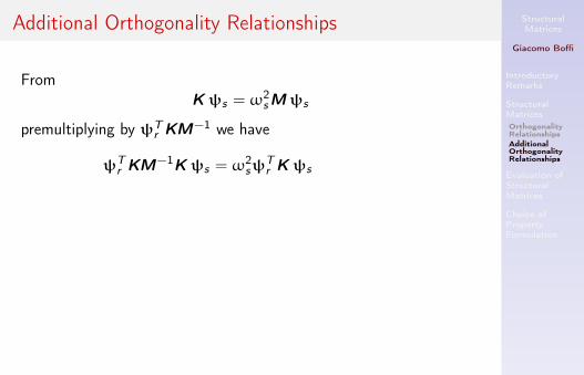
Additional Orthogonality Relationships
FromK ψs = ω
2sM ψs
premultiplying by ψTr KM−1 we have
ψTr KM−1K ψs = ω
2sψ
Tr K ψs
= δrsω4rMr ,
premultiplying the first equation by ψTr KM−1KM−1
ψTr KM−1KM−1K ψs = ω
2sψ
Tr KM−1K ψs = δrsω
6rMr
and, generalizing,
ψTr
(KM−1)b K ψs = δrs
(ω2
r
)b+1Mr .

StructuralMatrices
Giacomo Boffi
IntroductoryRemarks
StructuralMatricesOrthogonalityRelationshipsAdditionalOrthogonalityRelationships
Evaluation ofStructuralMatrices
Choice ofPropertyFormulation
Additional Orthogonality Relationships
FromK ψs = ω
2sM ψs
premultiplying by ψTr KM−1 we have
ψTr KM−1K ψs = ω
2sψ
Tr K ψs = δrsω
4rMr ,
premultiplying the first equation by ψTr KM−1KM−1
ψTr KM−1KM−1K ψs = ω
2sψ
Tr KM−1K ψs =
δrsω6rMr
and, generalizing,
ψTr
(KM−1)b K ψs = δrs
(ω2
r
)b+1Mr .

StructuralMatrices
Giacomo Boffi
IntroductoryRemarks
StructuralMatricesOrthogonalityRelationshipsAdditionalOrthogonalityRelationships
Evaluation ofStructuralMatrices
Choice ofPropertyFormulation
Additional Orthogonality Relationships
FromK ψs = ω
2sM ψs
premultiplying by ψTr KM−1 we have
ψTr KM−1K ψs = ω
2sψ
Tr K ψs = δrsω
4rMr ,
premultiplying the first equation by ψTr KM−1KM−1
ψTr KM−1KM−1K ψs = ω
2sψ
Tr KM−1K ψs = δrsω
6rMr
and, generalizing,
ψTr
(KM−1)b K ψs = δrs
(ω2
r
)b+1Mr .

StructuralMatrices
Giacomo Boffi
IntroductoryRemarks
StructuralMatricesOrthogonalityRelationshipsAdditionalOrthogonalityRelationships
Evaluation ofStructuralMatrices
Choice ofPropertyFormulation
Additional Orthogonality Relationships
FromK ψs = ω
2sM ψs
premultiplying by ψTr KM−1 we have
ψTr KM−1K ψs = ω
2sψ
Tr K ψs = δrsω
4rMr ,
premultiplying the first equation by ψTr KM−1KM−1
ψTr KM−1KM−1K ψs = ω
2sψ
Tr KM−1K ψs = δrsω
6rMr
and, generalizing,
ψTr
(KM−1)b K ψs = δrs
(ω2
r
)b+1Mr .
StructuralMatrices
Giacomo Boffi
IntroductoryRemarks
StructuralMatricesOrthogonalityRelationshipsAdditionalOrthogonalityRelationships
Evaluation ofStructuralMatrices
Choice ofPropertyFormulation
Additional Relationships, 2
FromM ψs = ω
−2s K ψs
premultiplying by ψTr MK−1 we have
ψTr MK−1M ψs = ω
−2s ψ
Tr M ψs =
δrsMs
ω2s
premultiplying the first eq. by ψTr
(MK−1
)2 we have
ψTr
(MK−1)2 M ψs = ω
−2s ψ
Tr MK−1M ψs = δrs
Ms
ω4s
and, generalizing,
ψTr
(MK−1)b M ψs = δrs
Ms
ω2sb
StructuralMatrices
Giacomo Boffi
IntroductoryRemarks
StructuralMatricesOrthogonalityRelationshipsAdditionalOrthogonalityRelationships
Evaluation ofStructuralMatrices
Choice ofPropertyFormulation
Additional Relationships, 2
FromM ψs = ω
−2s K ψs
premultiplying by ψTr MK−1 we have
ψTr MK−1M ψs = ω
−2s ψ
Tr M ψs = δrs
Ms
ω2s
premultiplying the first eq. by ψTr
(MK−1
)2 we have
ψTr
(MK−1)2 M ψs = ω
−2s ψ
Tr MK−1M ψs = δrs
Ms
ω4s
and, generalizing,
ψTr
(MK−1)b M ψs = δrs
Ms
ω2sb

StructuralMatrices
Giacomo Boffi
IntroductoryRemarks
StructuralMatricesOrthogonalityRelationshipsAdditionalOrthogonalityRelationships
Evaluation ofStructuralMatrices
Choice ofPropertyFormulation
Additional Relationships, 2
FromM ψs = ω
−2s K ψs
premultiplying by ψTr MK−1 we have
ψTr MK−1M ψs = ω
−2s ψ
Tr M ψs = δrs
Ms
ω2s
premultiplying the first eq. by ψTr
(MK−1
)2 we have
ψTr
(MK−1)2 M ψs = ω
−2s ψ
Tr MK−1M ψs =
δrsMs
ω4s
and, generalizing,
ψTr
(MK−1)b M ψs = δrs
Ms
ω2sb

StructuralMatrices
Giacomo Boffi
IntroductoryRemarks
StructuralMatricesOrthogonalityRelationshipsAdditionalOrthogonalityRelationships
Evaluation ofStructuralMatrices
Choice ofPropertyFormulation
Additional Relationships, 2
FromM ψs = ω
−2s K ψs
premultiplying by ψTr MK−1 we have
ψTr MK−1M ψs = ω
−2s ψ
Tr M ψs = δrs
Ms
ω2s
premultiplying the first eq. by ψTr
(MK−1
)2 we have
ψTr
(MK−1)2 M ψs = ω
−2s ψ
Tr MK−1M ψs = δrs
Ms
ω4s
and, generalizing,
ψTr
(MK−1)b M ψs = δrs
Ms
ω2sb

StructuralMatrices
Giacomo Boffi
IntroductoryRemarks
StructuralMatricesOrthogonalityRelationshipsAdditionalOrthogonalityRelationships
Evaluation ofStructuralMatrices
Choice ofPropertyFormulation
Additional Relationships, 2
FromM ψs = ω
−2s K ψs
premultiplying by ψTr MK−1 we have
ψTr MK−1M ψs = ω
−2s ψ
Tr M ψs = δrs
Ms
ω2s
premultiplying the first eq. by ψTr
(MK−1
)2 we have
ψTr
(MK−1)2 M ψs = ω
−2s ψ
Tr MK−1M ψs = δrs
Ms
ω4s
and, generalizing,
ψTr
(MK−1)b M ψs = δrs
Ms
ω2sb

StructuralMatrices
Giacomo Boffi
IntroductoryRemarks
StructuralMatricesOrthogonalityRelationshipsAdditionalOrthogonalityRelationships
Evaluation ofStructuralMatrices
Choice ofPropertyFormulation
Additional Relationships, 3
Defining Xrs(k) = ψTr M
(M−1K
)kψs we have
Xrs(0) = ψTr Mψs = δrs
(ω2
s
)0Ms
Xrs(1) = ψTr Kψs = δrs
(ω2
s
)1Ms
Xrs(2) = ψTr
(KM−1
)1 Kψs = δrs(ω2
s
)2Ms
· · ·Xrs(n) = ψ
Tr
(KM−1
)n−1 Kψs = δrs(ω2
s
)nMs
Observing that(M−1K
)−1=
(K−1M
)1
Xrs(−1) = ψT
r
(MK−1
)1 M ψs = δrs(ω2
s
)−1Ms
· · ·Xrs(−n) = ψT
r
(MK−1
)n M ψs = δrs(ω2
s
)−nMs
finallyXrs(k) = δrsω
2ks Ms for k = −∞, . . . ,∞.

Introductory Remarks
Structural Matrices
Evaluation of Structural MatricesFlexibility MatrixExampleStiffness MatrixMass MatrixDamping MatrixGeometric StiffnessExternal Loading
Choice of Property Formulation

StructuralMatrices
Giacomo Boffi
IntroductoryRemarks
StructuralMatrices
Evaluation ofStructuralMatricesFlexibility MatrixExampleStiffness MatrixMass MatrixDamping MatrixGeometricStiffnessExternal Loading
Choice ofPropertyFormulation
Flexibility
Given a system whose state is determined by the generalizeddisplacements xj of a set of nodes, we define the flexibility coefficientfjk as the deflection, in direction of xj , due to the application of aunit force in correspondance of the displacement xk .The matrix F =
[fjk]
is the flexibility matrix.
In general, the dynamic degrees of freedom correspond to the pointswhere there is
I application of external forces and/orI presence of inertial forces.
Given a load vector p ={pk
}, the displacementent xj is
xj =∑
fjkpk
or, in vector notation,x = F p

StructuralMatrices
Giacomo Boffi
IntroductoryRemarks
StructuralMatrices
Evaluation ofStructuralMatricesFlexibility MatrixExampleStiffness MatrixMass MatrixDamping MatrixGeometricStiffnessExternal Loading
Choice ofPropertyFormulation
Flexibility
Given a system whose state is determined by the generalizeddisplacements xj of a set of nodes, we define the flexibility coefficientfjk as the deflection, in direction of xj , due to the application of aunit force in correspondance of the displacement xk .The matrix F =
[fjk]
is the flexibility matrix.In general, the dynamic degrees of freedom correspond to the pointswhere there is
I application of external forces and/orI presence of inertial forces.
Given a load vector p ={pk
}, the displacementent xj is
xj =∑
fjkpk
or, in vector notation,x = F p

StructuralMatrices
Giacomo Boffi
IntroductoryRemarks
StructuralMatrices
Evaluation ofStructuralMatricesFlexibility MatrixExampleStiffness MatrixMass MatrixDamping MatrixGeometricStiffnessExternal Loading
Choice ofPropertyFormulation
Example
a b
m, J
x1
x2
1
1
f22
f11
f21
f12
The dynamical system The degrees of freedom
Displacements due to p1 = 1 and due to p2 = 1.
StructuralMatrices
Giacomo Boffi
IntroductoryRemarks
StructuralMatrices
Evaluation ofStructuralMatricesFlexibility MatrixExampleStiffness MatrixMass MatrixDamping MatrixGeometricStiffnessExternal Loading
Choice ofPropertyFormulation
Elastic Forces
Momentarily disregarding inertial effects, each node shall be inequilibrium under the action of the external forces and the elasticforces, hence taking into accounts all the nodes, all the externalforces and all the elastic forces it is possible to write the vectorequation of equilibrium
p = fS
and, substituting in the previos vector expression of thedisplacements
x = F fS

StructuralMatrices
Giacomo Boffi
IntroductoryRemarks
StructuralMatrices
Evaluation ofStructuralMatricesFlexibility MatrixExampleStiffness MatrixStrain EnergySymmetryDirectAssemblageExampleMass MatrixDamping MatrixGeometricStiffnessExternal Loading
Choice ofPropertyFormulation
Stiffness Matrix
The stiffness matrix K can be simply defined as the inverse of theflexibility matrix F ,
K = F−1.
As an alternative definition, consider an unary vector ofdisplacements,
e(i) ={δij
}, j = 1, . . . ,N,
and the vector of nodal forces ki that, applied to the structure,produces the displacements e(i)
F ki = e(i), i = 1, . . . ,N.

StructuralMatrices
Giacomo Boffi
IntroductoryRemarks
StructuralMatrices
Evaluation ofStructuralMatricesFlexibility MatrixExampleStiffness MatrixStrain EnergySymmetryDirectAssemblageExampleMass MatrixDamping MatrixGeometricStiffnessExternal Loading
Choice ofPropertyFormulation
Stiffness Matrix
Collecting all the ordered e(i) in a matrix E , it is clear that E ≡ Iand we have, writing all the equations at once,
F[ki]=
[e(i)
]= E = I .
Collecting the ordered force vectors in a matrix K =[~ki]
we have
FK = I , ⇒ K = F−1,
giving a physical interpretation to the columns of the stiffness matrix.
Finally, writing the nodal equilibrium, we have
p = fS = K x .

StructuralMatrices
Giacomo Boffi
IntroductoryRemarks
StructuralMatrices
Evaluation ofStructuralMatricesFlexibility MatrixExampleStiffness MatrixStrain EnergySymmetryDirectAssemblageExampleMass MatrixDamping MatrixGeometricStiffnessExternal Loading
Choice ofPropertyFormulation
Strain Energy
The elastic strain energy V can be written in terms of displacementsand external forces,
V =12pTx =
12
pT F p︸︷︷︸
x
,
xTK︸ ︷︷ ︸pT
x .
Because the elastic strain energy of a stable system is always greaterthan zero, K is a positive definite matrix.
On the other hand, for an unstable system, think of a compressedbeam, there are displacement patterns that are associated to zerostrain energy.

StructuralMatrices
Giacomo Boffi
IntroductoryRemarks
StructuralMatrices
Evaluation ofStructuralMatricesFlexibility MatrixExampleStiffness MatrixStrain EnergySymmetryDirectAssemblageExampleMass MatrixDamping MatrixGeometricStiffnessExternal Loading
Choice ofPropertyFormulation
Symmetry
Two sets of loads pA and pB are applied, one after the other, to anelastic system; the work done is
VAB =12pAT
xA + pATxB +
12pBT
xB .
If we revert the order of application the work is
VBA =12pBT
xB + pBTxA +
12pAT
xA.
The total work being independent of the order of loading,
pATxB = pBT
xA.

StructuralMatrices
Giacomo Boffi
IntroductoryRemarks
StructuralMatrices
Evaluation ofStructuralMatricesFlexibility MatrixExampleStiffness MatrixStrain EnergySymmetryDirectAssemblageExampleMass MatrixDamping MatrixGeometricStiffnessExternal Loading
Choice ofPropertyFormulation
Symmetry, 2
Expressing the displacements in terms of F ,
pATF pB = pBT
FpA,
both terms are scalars so we can write
pATF pB =
(pBT
FpA)T
= pATFT pB .
Because this equation holds for every p, we conclude that
F = FT .
The inverse of a symmetric matrix is symmetric, hence
K = KT .

StructuralMatrices
Giacomo Boffi
IntroductoryRemarks
StructuralMatrices
Evaluation ofStructuralMatricesFlexibility MatrixExampleStiffness MatrixStrain EnergySymmetryDirectAssemblageExampleMass MatrixDamping MatrixGeometricStiffnessExternal Loading
Choice ofPropertyFormulation
A practical consideration
For the kind of structures we mostly deal with in our examples,problems, exercises and assignments, that is simple structures, it isusually convenient to compute first the flexibility matrix applying thePrinciple of Virtual Displacements and later the stiffness matrix,using inversion,
K = F−1.
On the other hand, the PVD approach cannot work in practice forreal structures, because the number of degrees of freedom necessaryto model the structural behaviour exceeds our ability to apply thePVD...The stiffness matrix for large, complex structures to constructdifferent methods required are.E.g., the Finite Element Method.

StructuralMatrices
Giacomo Boffi
IntroductoryRemarks
StructuralMatrices
Evaluation ofStructuralMatricesFlexibility MatrixExampleStiffness MatrixStrain EnergySymmetryDirectAssemblageExampleMass MatrixDamping MatrixGeometricStiffnessExternal Loading
Choice ofPropertyFormulation
A practical consideration
For the kind of structures we mostly deal with in our examples,problems, exercises and assignments, that is simple structures, it isusually convenient to compute first the flexibility matrix applying thePrinciple of Virtual Displacements and later the stiffness matrix,using inversion,
K = F−1.
On the other hand, the PVD approach cannot work in practice forreal structures, because the number of degrees of freedom necessaryto model the structural behaviour exceeds our ability to apply thePVD...The stiffness matrix for large, complex structures to constructdifferent methods required are.
E.g., the Finite Element Method.
StructuralMatrices
Giacomo Boffi
IntroductoryRemarks
StructuralMatrices
Evaluation ofStructuralMatricesFlexibility MatrixExampleStiffness MatrixStrain EnergySymmetryDirectAssemblageExampleMass MatrixDamping MatrixGeometricStiffnessExternal Loading
Choice ofPropertyFormulation
A practical consideration
For the kind of structures we mostly deal with in our examples,problems, exercises and assignments, that is simple structures, it isusually convenient to compute first the flexibility matrix applying thePrinciple of Virtual Displacements and later the stiffness matrix,using inversion,
K = F−1.
On the other hand, the PVD approach cannot work in practice forreal structures, because the number of degrees of freedom necessaryto model the structural behaviour exceeds our ability to apply thePVD...The stiffness matrix for large, complex structures to constructdifferent methods required are.E.g., the Finite Element Method.

StructuralMatrices
Giacomo Boffi
IntroductoryRemarks
StructuralMatrices
Evaluation ofStructuralMatricesFlexibility MatrixExampleStiffness MatrixStrain EnergySymmetryDirectAssemblageExampleMass MatrixDamping MatrixGeometricStiffnessExternal Loading
Choice ofPropertyFormulation
FEM
The most common procedure to construct the matrices that describe thebehaviour of a complex system is the Finite Element Method, or FEM.The procedure can be sketched in the following terms:
I the structure is subdivided in non-overlapping portions, the finiteelements, bounded by nodes, connected by the same nodes,
I the state of the structure can be described in terms of a vector x ofgeneralized nodal displacements,
I there is a mapping between element and structure DOF’s, iel 7→ r ,
I the element stiffness matrix, Kel establishes a linear relation betweenan element nodal displacements and forces,
I for each FE, all local kij ’s are contributed to the global stiffness krs ’s,with i 7→ r and j 7→ s, taking in due consideration differencesbetween local and global systems of reference.
Note that in the r -th global equation of equilibrium we have internal forcescaused by the nodal displacements of the FE that have nodes iel such thatiel 7→ r , thus implying that global K is a banded matrix.

StructuralMatrices
Giacomo Boffi
IntroductoryRemarks
StructuralMatrices
Evaluation ofStructuralMatricesFlexibility MatrixExampleStiffness MatrixStrain EnergySymmetryDirectAssemblageExampleMass MatrixDamping MatrixGeometricStiffnessExternal Loading
Choice ofPropertyFormulation
Example
Consider a 2-D inextensible beam element, that has 4 DOF, namelytwo transverse end displacements x1, x2 and two end rotations, x3,x4. The element stiffness is computed using 4 shape functions φi ,the transverse displacement being v(s) =
∑i φi (s) xi , 0 6 s 6 L,
the different φi are such all end displacements or rotation are zero,except the one corresponding to index i .The shape functions for a beam are
φ1(s) = 1 − 3( sL
)2+ 2
( sL
)3, φ2(s) = 3
( sL
)2− 2
( sL
)3,
φ3(s) =( sL
)− 2
( sL
)2+( sL
)3φ4(s) = −
( sL
)2+( sL
)3.

StructuralMatrices
Giacomo Boffi
IntroductoryRemarks
StructuralMatrices
Evaluation ofStructuralMatricesFlexibility MatrixExampleStiffness MatrixStrain EnergySymmetryDirectAssemblageExampleMass MatrixDamping MatrixGeometricStiffnessExternal Loading
Choice ofPropertyFormulation
Example, 2
The element stiffness coefficients can be computed using, what else,the PVD: we compute the external virtual work done by a variationδ xi by the force due to a unit displacement xj , that is kij ,
δWext = δ xi kij ,
the virtual internal work is the work done by the variation of thecurvature, δ xiφ′′
i (s) by the bending moment associated with a unitxj , φ′′
j (s)EJ(s),
δWint =
∫L0δ xiφ
′′i (s)φ
′′j (s)EJ(s) ds.
StructuralMatrices
Giacomo Boffi
IntroductoryRemarks
StructuralMatrices
Evaluation ofStructuralMatricesFlexibility MatrixExampleStiffness MatrixStrain EnergySymmetryDirectAssemblageExampleMass MatrixDamping MatrixGeometricStiffnessExternal Loading
Choice ofPropertyFormulation
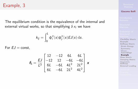
Example, 3
The equilibrium condition is the equivalence of the internal andexternal virtual works, so that simplifying δ xi we have
kij =
∫L0φ′′i (s)φ
′′j (s)EJ(s) ds.
For EJ = const,
fS =EJ
L3
12 −12 6L 6L−12 12 −6L −6L6L −6L 4L2 2L2
6L −6L 2L2 4L2
x
StructuralMatrices
Giacomo Boffi
IntroductoryRemarks
StructuralMatrices
Evaluation ofStructuralMatricesFlexibility MatrixExampleStiffness MatrixStrain EnergySymmetryDirectAssemblageExampleMass MatrixDamping MatrixGeometricStiffnessExternal Loading
Choice ofPropertyFormulation
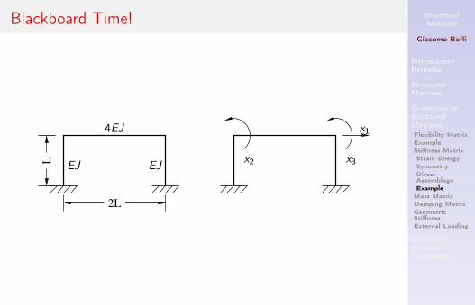
Blackboard Time!
L
2L
EJ EJ
4EJ
x2 x3
x1

StructuralMatrices
Giacomo Boffi
IntroductoryRemarks
StructuralMatrices
Evaluation ofStructuralMatricesFlexibility MatrixExampleStiffness MatrixMass MatrixConsistent MassMatrixDiscussionDamping MatrixGeometricStiffnessExternal Loading
Choice ofPropertyFormulation
Mass Matrix
The mass matrix maps the nodal accelerations to nodal inertialforces, and the most common assumption is to concentrate all themasses in nodal point masses, without rotational inertia, computedlumping a fraction of each element mass (or a fraction of thesupported mass) on all its bounding nodes.This procedure leads to a so called lumped mass matrix, a diagonalmatrix with diagonal elements greater than zero for all thetranslational degrees of freedom and diagonal elements equal to zerofor angular degrees of freedom.

StructuralMatrices
Giacomo Boffi
IntroductoryRemarks
StructuralMatrices
Evaluation ofStructuralMatricesFlexibility MatrixExampleStiffness MatrixMass MatrixConsistent MassMatrixDiscussionDamping MatrixGeometricStiffnessExternal Loading
Choice ofPropertyFormulation
Mass Matrix
The mass matrix is definite positive only if all the structure DOF’sare translational degrees of freedom, otherwise M is semi-definitepositive and the eigenvalue procedure is not directly applicable. Thisproblem can be overcome either by using a consistent mass matrix orusing the static condensation procedure.

StructuralMatrices
Giacomo Boffi
IntroductoryRemarks
StructuralMatrices
Evaluation ofStructuralMatricesFlexibility MatrixExampleStiffness MatrixMass MatrixConsistent MassMatrixDiscussionDamping MatrixGeometricStiffnessExternal Loading
Choice ofPropertyFormulation
Consistent Mass Matrix
A consistent mass matrix is built using the rigorous FEM procedure, computingthe nodal reactions that equilibrate the distributed inertial forces that develop inthe element due to a linear combination of inertial forces.Using our beam example as a reference, consider the inertial forces associatedwith a single nodal acceleration xj , fI,j(s) = m(s)φj (s)xj and denote with mij xjthe reaction associated with the i-nth degree of freedom of the element, by thePVD
δ ximij xj =
∫δ xiφi (s)m(s)φj (s)ds xj
simplifying
mij =
∫m(s)φi (s)φj (s)ds.
For m(s) = m = const.
fI =mL
420
156 54 22L −13L54 156 13L −22L22L 13L 4L2 −3L2
−13L −22L −3L2 4L2
x

StructuralMatrices
Giacomo Boffi
IntroductoryRemarks
StructuralMatrices
Evaluation ofStructuralMatricesFlexibility MatrixExampleStiffness MatrixMass MatrixConsistent MassMatrixDiscussionDamping MatrixGeometricStiffnessExternal Loading
Choice ofPropertyFormulation
Consistent Mass Matrix, 2
ProI some convergence theorem of FEM theory holds only if the
mass matrix is consistent,I sligtly more accurate results,I no need for static condensation.
ContraI M is no more diagonal, heavy computational aggravation,I static condensation is computationally beneficial, inasmuch it
reduces the global number of degrees of freedom.

StructuralMatrices
Giacomo Boffi
IntroductoryRemarks
StructuralMatrices
Evaluation ofStructuralMatricesFlexibility MatrixExampleStiffness MatrixMass MatrixDamping MatrixExampleGeometricStiffnessExternal Loading
Choice ofPropertyFormulation
Damping Matrix
For each element cij =∫c(s)φi (s)φj(s) ds and the damping matrix
C can be assembled from element contributions.
However, using the FEM C? = ΨTC Ψ is not diagonal and themodal equations are no more uncoupled!The alternative is to write directly the global damping matrix, interms of the underdetermined coefficients cb,
C =∑b
cbM(M−1K
)b.

StructuralMatrices
Giacomo Boffi
IntroductoryRemarks
StructuralMatrices
Evaluation ofStructuralMatricesFlexibility MatrixExampleStiffness MatrixMass MatrixDamping MatrixExampleGeometricStiffnessExternal Loading
Choice ofPropertyFormulation
Damping Matrix
For each element cij =∫c(s)φi (s)φj(s) ds and the damping matrix
C can be assembled from element contributions.However, using the FEM C? = ΨTC Ψ is not diagonal and themodal equations are no more uncoupled!
The alternative is to write directly the global damping matrix, interms of the underdetermined coefficients cb,
C =∑b
cbM(M−1K
)b.

StructuralMatrices
Giacomo Boffi
IntroductoryRemarks
StructuralMatrices
Evaluation ofStructuralMatricesFlexibility MatrixExampleStiffness MatrixMass MatrixDamping MatrixExampleGeometricStiffnessExternal Loading
Choice ofPropertyFormulation
Damping Matrix
For each element cij =∫c(s)φi (s)φj(s) ds and the damping matrix
C can be assembled from element contributions.However, using the FEM C? = ΨTC Ψ is not diagonal and themodal equations are no more uncoupled!The alternative is to write directly the global damping matrix, interms of the underdetermined coefficients cb,
C =∑b
cbM(M−1K
)b.

StructuralMatrices
Giacomo Boffi
IntroductoryRemarks
StructuralMatrices
Evaluation ofStructuralMatricesFlexibility MatrixExampleStiffness MatrixMass MatrixDamping MatrixExampleGeometricStiffnessExternal Loading
Choice ofPropertyFormulation
Damping Matrix
With our definition of C ,
C =∑b
cbM(M−1K
)b,
assuming normalized eigenvectors, we can write the individualcomponent of C? = ΨTC Ψ
c?ij = ψTi C ψj = δij
∑b
cbω2bj
due to the additional orthogonality relations, we recognize that nowC? is a diagonal matrix.
Introducing the modal damping Cj we have
Cj = ψTj C ψj =
∑b
cbω2bj = 2ζjωj
and we can write a system of linear equations in the cb.

StructuralMatrices
Giacomo Boffi
IntroductoryRemarks
StructuralMatrices
Evaluation ofStructuralMatricesFlexibility MatrixExampleStiffness MatrixMass MatrixDamping MatrixExampleGeometricStiffnessExternal Loading
Choice ofPropertyFormulation
Damping Matrix
With our definition of C ,
C =∑b
cbM(M−1K
)b,
assuming normalized eigenvectors, we can write the individualcomponent of C? = ΨTC Ψ
c?ij = ψTi C ψj = δij
∑b
cbω2bj
due to the additional orthogonality relations, we recognize that nowC? is a diagonal matrix.Introducing the modal damping Cj we have
Cj = ψTj C ψj =
∑b
cbω2bj = 2ζjωj
and we can write a system of linear equations in the cb.

StructuralMatrices
Giacomo Boffi
IntroductoryRemarks
StructuralMatrices
Evaluation ofStructuralMatricesFlexibility MatrixExampleStiffness MatrixMass MatrixDamping MatrixExampleGeometricStiffnessExternal Loading
Choice ofPropertyFormulation
Example
We want a fixed, 5% damping ratio for the first three modes, takingnote that the modal equation of motion is
qi + 2ζiωi qi +ω2i qi = p?i
UsingC = c0M + c1K + c2KM−1K
we have
2 × 0.05
ω1ω2ω3
=
1 ω21 ω4
11 ω2
2 ω42
1 ω23 ω4
3
c0c1c2
Solving for the c’s and substituting above, the resulting dampingmatrix is orthogonal to every eigenvector of the system, for the firstthree modes, leads to a modal damping ratio that is equal to 5%.

StructuralMatrices
Giacomo Boffi
IntroductoryRemarks
StructuralMatrices
Evaluation ofStructuralMatricesFlexibility MatrixExampleStiffness MatrixMass MatrixDamping MatrixExampleGeometricStiffnessExternal Loading
Choice ofPropertyFormulation
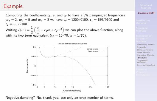
ExampleComputing the coefficients c0, c1 and c2 to have a 5% damping at frequenciesω1 = 2, ω2 = 5 and ω3 = 8 we have c0 = 1200/9100, c1 = 159/9100 andc2 = −1/9100.
Writing ζ(ω) =12
( c0ω
+ c1ω+ c2ω3)
we can plot the above function, along
with its two term equivalent (c0 = 10/70, c1 = 1/70).
-0.1
-0.05
0
0.05
0.1
0 2 5 8 10 15 20
Dam
pin
g r
ati
o
Circular frequency
Two and three terms solutions
three termstwo terms
Negative damping? No, thank you: use only an even number of terms.
StructuralMatrices
Giacomo Boffi
IntroductoryRemarks
StructuralMatrices
Evaluation ofStructuralMatricesFlexibility MatrixExampleStiffness MatrixMass MatrixDamping MatrixExampleGeometricStiffnessExternal Loading
Choice ofPropertyFormulation
ExampleComputing the coefficients c0, c1 and c2 to have a 5% damping at frequenciesω1 = 2, ω2 = 5 and ω3 = 8 we have c0 = 1200/9100, c1 = 159/9100 andc2 = −1/9100.
Writing ζ(ω) =12
( c0ω
+ c1ω+ c2ω3)
we can plot the above function, along
with its two term equivalent (c0 = 10/70, c1 = 1/70).
-0.1
-0.05
0
0.05
0.1
0 2 5 8 10 15 20
Dam
pin
g r
ati
o
Circular frequency
Two and three terms solutions
three termstwo terms
Negative damping? No, thank you: use only an even number of terms.
StructuralMatrices
Giacomo Boffi
IntroductoryRemarks
StructuralMatrices
Evaluation ofStructuralMatricesFlexibility MatrixExampleStiffness MatrixMass MatrixDamping MatrixGeometricStiffnessExternal Loading
Choice ofPropertyFormulation
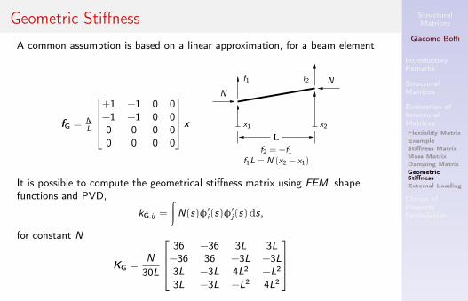
Geometric StiffnessA common assumption is based on a linear approximation, for a beam element
fG = NL
+1 −1 0 0−1 +1 0 00 0 0 00 0 0 0
xL
x1 x2
N
Nf1 f2
f2 = −f1f1L = N (x2 − x1)
It is possible to compute the geometrical stiffness matrix using FEM, shapefunctions and PVD,
kG,ij =
∫N(s)φ′
i (s)φ′j (s)ds,
for constant N
KG =N
30L
36 −36 3L 3L−36 36 −3L −3L3L −3L 4L2 −L2
3L −3L −L2 4L2

StructuralMatrices
Giacomo Boffi
IntroductoryRemarks
StructuralMatrices
Evaluation ofStructuralMatricesFlexibility MatrixExampleStiffness MatrixMass MatrixDamping MatrixGeometricStiffnessExternal Loading
Choice ofPropertyFormulation
External Loadings
Following the same line of reasoning that we applied to find nodalinertial forces, by the PVD and the use of shape functions we have
pi (t) =
∫p(s, t)φi (s) ds.
For a constant, uniform load p(s, t) = p = const, applied on a beamelement,
p = pL{1
212
L12 − L
12
}T

Introductory Remarks
Structural Matrices
Evaluation of Structural Matrices
Choice of Property FormulationStatic CondensationExample

StructuralMatrices
Giacomo Boffi
IntroductoryRemarks
StructuralMatrices
Evaluation ofStructuralMatrices
Choice ofPropertyFormulationStaticCondensationExample
Choice of Property Formulation
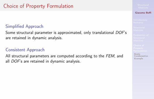
Simplified ApproachSome structural parameter is approximated, only translational DOF’sare retained in dynamic analysis.
Consistent ApproachAll structural parameters are computed according to the FEM, andall DOF’s are retained in dynamic analysis.If we choose a simplified approach, we must use a procedure toremove unneeded structural DOF’s from the model that we use forthe dynamic analysis.Enter the Static Condensation Method.
StructuralMatrices
Giacomo Boffi
IntroductoryRemarks
StructuralMatrices
Evaluation ofStructuralMatrices
Choice ofPropertyFormulationStaticCondensationExample
Choice of Property Formulation
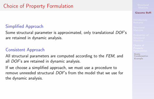
Simplified ApproachSome structural parameter is approximated, only translational DOF’sare retained in dynamic analysis.
Consistent ApproachAll structural parameters are computed according to the FEM, andall DOF’s are retained in dynamic analysis.
If we choose a simplified approach, we must use a procedure toremove unneeded structural DOF’s from the model that we use forthe dynamic analysis.Enter the Static Condensation Method.
StructuralMatrices
Giacomo Boffi
IntroductoryRemarks
StructuralMatrices
Evaluation ofStructuralMatrices
Choice ofPropertyFormulationStaticCondensationExample
Choice of Property Formulation
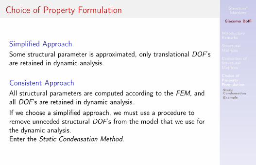
Simplified ApproachSome structural parameter is approximated, only translational DOF’sare retained in dynamic analysis.
Consistent ApproachAll structural parameters are computed according to the FEM, andall DOF’s are retained in dynamic analysis.If we choose a simplified approach, we must use a procedure toremove unneeded structural DOF’s from the model that we use forthe dynamic analysis.
Enter the Static Condensation Method.
StructuralMatrices
Giacomo Boffi
IntroductoryRemarks
StructuralMatrices
Evaluation ofStructuralMatrices
Choice ofPropertyFormulationStaticCondensationExample
Choice of Property Formulation
Simplified ApproachSome structural parameter is approximated, only translational DOF’sare retained in dynamic analysis.
Consistent ApproachAll structural parameters are computed according to the FEM, andall DOF’s are retained in dynamic analysis.If we choose a simplified approach, we must use a procedure toremove unneeded structural DOF’s from the model that we use forthe dynamic analysis.Enter the Static Condensation Method.

StructuralMatrices
Giacomo Boffi
IntroductoryRemarks
StructuralMatrices
Evaluation ofStructuralMatrices
Choice ofPropertyFormulationStaticCondensationExample
Static Condensation
We have, from a FEM analysis, a stiffnes matrix that uses all nodalDOF’s, and from the lumped mass procedure a mass matrix wereonly translational (and maybe a few rotational) DOF’s are blessedwith a non zero diagonal term.
In this case, we can always rearrange
and partition the displacement vector x in two subvectors: a) xA, allthe DOF’s that are associated with inertial forces and b) xB , all theremaining DOF’s not associated with inertial forces.
x ={xA xB
}T

StructuralMatrices
Giacomo Boffi
IntroductoryRemarks
StructuralMatrices
Evaluation ofStructuralMatrices
Choice ofPropertyFormulationStaticCondensationExample
Static Condensation
We have, from a FEM analysis, a stiffnes matrix that uses all nodalDOF’s, and from the lumped mass procedure a mass matrix wereonly translational (and maybe a few rotational) DOF’s are blessedwith a non zero diagonal term. In this case, we can always rearrange
and partition the displacement vector x in two subvectors: a) xA, allthe DOF’s that are associated with inertial forces and b) xB , all theremaining DOF’s not associated with inertial forces.
x ={xA xB
}T

StructuralMatrices
Giacomo Boffi
IntroductoryRemarks
StructuralMatrices
Evaluation ofStructuralMatrices
Choice ofPropertyFormulationStaticCondensationExample
Static Condensation, 2
After rearranging the DOF’s, we must rearrange also the rows(equations) and the columns (force contributions) in the structuralmatrices, and eventually partition the matrices so that{
fI0
}=
[MAA MAB
MBA MBB
]{xAxB
}fS =
[KAA KAB
KBA KBB
]{xAxB
}with
MBA = MTAB = 0, MBB = 0, KBA = KT
AB
Finally we rearrange the loadings vector and write...
StructuralMatrices
Giacomo Boffi
IntroductoryRemarks
StructuralMatrices
Evaluation ofStructuralMatrices
Choice ofPropertyFormulationStaticCondensationExample
Static Condensation, 2
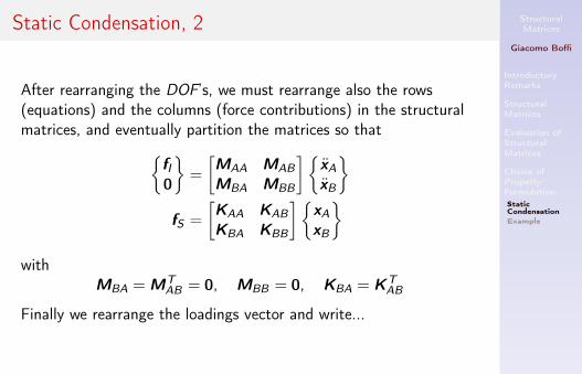
After rearranging the DOF’s, we must rearrange also the rows(equations) and the columns (force contributions) in the structuralmatrices, and eventually partition the matrices so that{
fI0
}=
[MAA MAB
MBA MBB
]{xAxB
}fS =
[KAA KAB
KBA KBB
]{xAxB
}with
MBA = MTAB = 0, MBB = 0, KBA = KT
AB
Finally we rearrange the loadings vector and write...

StructuralMatrices
Giacomo Boffi
IntroductoryRemarks
StructuralMatrices
Evaluation ofStructuralMatrices
Choice ofPropertyFormulationStaticCondensationExample
Static Condensation, 3
... the equation of dynamic equilibrium,
pA = MAAxA + MAB xB + KAAxA + KABxBpB = MBAxA + MBB xB + KBAxA + KBBxB
The terms in red are zero, so we can simplify
MAAxA + KAAxA + KABxB = pA
KBAxA + KBBxB = pB
solving for xB in the 2nd equation and substituting
xB = K−1BBpB − K−1
BBKBAxApA − KABK−1
BBpB = MAAxA +(KAA − KABK−1
BBKBA
)xA

StructuralMatrices
Giacomo Boffi
IntroductoryRemarks
StructuralMatrices
Evaluation ofStructuralMatrices
Choice ofPropertyFormulationStaticCondensationExample
Static Condensation, 3
... the equation of dynamic equilibrium,
pA = MAAxA + MAB xB + KAAxA + KABxBpB = MBAxA + MBB xB + KBAxA + KBBxB
The terms in red are zero, so we can simplify
MAAxA + KAAxA + KABxB = pA
KBAxA + KBBxB = pB
solving for xB in the 2nd equation and substituting
xB = K−1BBpB − K−1
BBKBAxApA − KABK−1
BBpB = MAAxA +(KAA − KABK−1
BBKBA
)xA
StructuralMatrices
Giacomo Boffi
IntroductoryRemarks
StructuralMatrices
Evaluation ofStructuralMatrices
Choice ofPropertyFormulationStaticCondensationExample
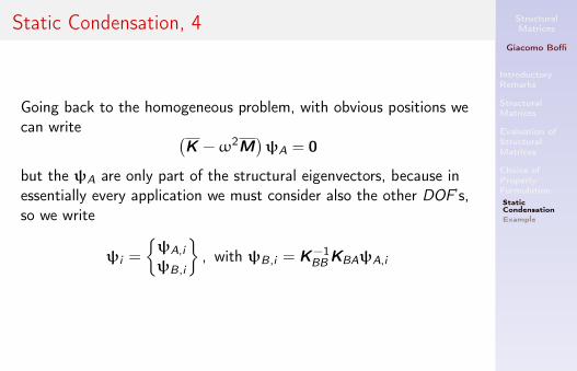
Static Condensation, 4
Going back to the homogeneous problem, with obvious positions wecan write (
K −ω2M)ψA = 0
but the ψA are only part of the structural eigenvectors, because inessentially every application we must consider also the other DOF’s,so we write
ψi =
{ψA,i
ψB,i
}, with ψB,i = K−1
BBKBAψA,i

StructuralMatrices
Giacomo Boffi
IntroductoryRemarks
StructuralMatrices
Evaluation ofStructuralMatrices
Choice ofPropertyFormulationStaticCondensationExample
Example
L
2L
EJ EJ
4EJx2 x3
x1
K = 2EJL3
12 3L 3L3L 6L2 2L2
3L 2L2 6L2
Disregarding the factor 2EJ/L3,
KBB = L2[6 22 6
],K−1
BB =1
32L2
[6 −2−2 6
],KAB =
[3L 3L
]The matrix K is
K =2EJL3
(12 − KABK−1
BBKTAB
)=
39EJ2L3