Structural Macroeconometrics

Chapter 6. Calibration

David N. DeJong Chetan Dave

Models are to be used, not believed.

Henri Theil, 1971, Principles of Econometrics, New York: Wiley.

1 Historical Origins and Philosophy

With their seminal analysis of business cycles, Kydland and Prescott (1982) capped

a paradigm shift in the conduct of empirical work in macroeconomics. They did so by

employing a methodology that enabled them to cast the DSGE model they analyzed as the

centerpiece of their empirical analysis. The analysis contributed towards the Nobel Prize in

Economics they received in 2004, and the methodology has come to be known as a calibration

exercise.1 Calibration not only remains a popular tool for analyzing DSGEs, but has also

served as the building block for subsequent methodologies developed towards this end. Thus

it provides a natural point of departure for our presentation of these methodologies.

While undoubtedly an empirical methodology, calibration is distinct from the branch of

econometrics under which theoretical models are represented as complete probability models

that can be estimated, tested, and used to generate predictions using formal statistical pro-

cedures. Haavelmo (1944) provided an early and forceful articulation of this latter approach

to econometrics, and in 1989 received the Nobel Prize in Economics �...for his clari�cation

of the probability theory foundations of econometrics and his analyses of simultaneous eco-

nomic structures.�(Bank of Sweden, 1989) Henceforth, we will refer to this as the probability

approach to econometrics.

1Speci�cally, Kydland and Prescott received the Nobel Prize �for their contributions to dynamic macro-economics: the time consistency of economic policy and the driving forces behind business cycles.�(Bank ofSweden, 2004)

1

Regarding Haavelmo�s �... analyses of simultaneous economic structures�, otherwise

known as systems-of-equations models, at the time of his work this was the most sophisti-

cated class of structural models that could be subjected to formal empirical analysis. As

characterized by Koopmans (1949), such models include equations falling into one of four

classes: identities (e.g., the national income accounting identity); institutional rules (e.g.,

tax rates); technology constraints (e.g., a production function); and behavioral equations

(e.g., a consumption function relating consumption to disposable income).2

This latter class of equations distinguishes systems-of-equations models from DSGE mod-

els. Behavioral equations cast endogenous variables as ad hoc functions of additional vari-

ables included in the model. An important objective in designing these speci�cations is to

capture relationships between variables observed from historical data. Indeed, econometric

implementations of such models proceed under the assumption that the parameters of the

behavioral equations are �xed, and thus may be estimated using historical data; the esti-

mated models are then used to address quantitative questions. Such analyses represented

state-of-the-art practice in econometrics into the 1970s.

In place of behavioral equations, DSGE models feature equations that re�ect the pur-

suit of explicit objectives (e.g., the maximization of lifetime utility) by purposeful decision

makers (e.g., representative households). For example, the RBC model presented in Chap-

ter 5 features two such equations: the intratemporal optimality condition that determines

the labor-leisure trade-o¤; and the intertemporal optimality condition that determines the

consumption-investment trade-o¤. The parameters in these equations either re�ect the pref-

erences of the decision maker (e.g., discount factors, intertemporal elasticities of substitution,

2For a textbook presentation of systems-of-equations models, see Sargent (1987).

2

etc.) or features of their environment (e.g., capital�s share of labor in the production tech-

nology).

Two important developments ultimately ended the predominance of the systems-of-

equations approach. The �rst was empirical: systems�of-equations models su¤ered �...spec-

tacular predictive failure...� in the policy guidance they provided during the episode of

stag�ation experienced during the early 1970s (Kydland and Prescott, 1991a, p. 166). Quot-

ing Lucas and Sargent (1979):

In the present decade, the U.S. economy has undergone its �rst major de-

pression since the 1930�s, to the accompaniment of in�ation rates in excess of 10

percent per annum.... These events ... were accompanied by massive government

budget de�cits and high rates of monetary expansion, policies which, although

bearing an admitted risk of in�ation, promised according to modern Keynesian

doctrine rapid real growth and low rates of unemployment. That these predic-

tions were wildly incorrect and that the doctrine on which they were based is

fundamentally �awed are now simple matters of fact, involving no novelties in

economic theory. [p. 1]

The second development was theoretical: the underlying assumption that the parameters

of behavioral equations in such models are �xed was recognized as being inconsistent with

optimizing behavior on the part of purposeful decision makers. This is the thrust of Lucas�

(1976) critique of policy evaluation based on systems-of-equations models:

... given that the structure of an econometric model consists of optimal deci-

sion rules of economic agents, and that optimal decision rules vary systematically

3

with changes in the structure of series relevant to the decision maker, it follows

that any change in policy will systematically alter the structure of econometric

models. [p. 41]

Or as summarized by Lucas and Sargent (1979):

The casual treatment of expectations is not a peripheral problem in these

models, for the role of expectations is pervasive in them and exerts a massive

in�uence on their dynamic properties.... The failure of existing models to derive

restrictions on expectations from any �rst principles grounded in economic theory

is a symptom of a deeper and more general failure to derive behavioral relation-

ships from any consistently posed dynamic optimization problem.... There are,

therefore, ... theoretical reasons for believing that the parameters identi�ed as

structural by current macroeconomic methods are not in fact structural. That

is, we see no reason to believe that these models have isolated structures which

will remain invariant across the class of interventions that �gure in contemporary

discussions of economic policy. [pp. 5-6]

In consequence, Lucas (1976) concludes that �... simulations using these models can, in

principle, provide no useful information as to the actual consequences of alternative economic

policies.�[p. 20] In turn, again referring to the predictive failure of these models during the

stag�ation episode of the 1970s, Lucas and Sargent (1979) conclude that �... the di¢ culties

are fatal : that modern macroeconomic models are of no value in guiding policy and that

this condition will not be remedied by modi�cations along any line which is currently being

pursued.�[p. 2]

4

Two leading reactions to these developments ensued. First, remaining in the tradition of

the probability approach to econometrics, the methodological contributions of Sims (1972)

and Hansen and Sargent (1980) made possible the imposition of theoretical discipline on

reduced-form models of macroeconomic activity. DSGE models featuring rational decision

makers provided the source of this discipline, and the form of the discipline most commonly

took the form of �cross-equation restrictions�imposed on vector autoregressive (VAR) mod-

els. This development represents an intermediate step towards the implementation of DSGE

models in empirical applications, since reduced-form models serve as the focal point of such

analyses. Moreover, early empirical applications spawned by this development proved to

be disappointing, as rejections of particular parametric implementations of the restrictions

were commonplace (e.g., see Hansen and Sargent, 1981; Hansen and Singleton 1982, 1983;

and Eichenbaum 1983). The second reaction was the development of the modern calibration

exercise.

In place of estimation and testing, the goal in a calibration exercise is to use a parameter-

ized structural model to address a speci�c quantitative question. The model is constructed

and parameterized subject to the constraint that it mimic features of the actual economy

that have been identi�ed a priori. Questions fall under two general headings. They may

involve the ability of the model to account for an additional set of features of the actual

economy; i.e., they may involve assessments of �t. Alternatively, they may involve assess-

ments of the theoretical implications of changes in economic policy. This characterization

stems from Kydland and Prescott (1991a, 1996), who traced the historical roots of the use

of calibration exercises as an empirical methodology, and outlined their view of what such

exercises entail.

5

Kydland and Prescott (1991a) identify calibration as embodying the approach to econo-

metrics articulated and practiced by Frisch (1933a,b). Regarding articulation, this is pro-

vided by Frisch�s (1933a) editorial opening the inaugural issue of the �agship journal of the

Econometric Society: Econometrica. As stated in its constitution, the main objective of the

Econometric Society is to

... promote studies that aim at a uni�cation of the theoretical-quantitative

and empirical-quantitative approach to economic problems and that are pen-

etrated by constructive and rigorous thinking.... Any activity which promises

ultimately to further such uni�cation of theoretical and factual studies in eco-

nomics shall be within the sphere of interest of the Society.�[p. 1]

Such studies personi�ed Frisch�s vision of econometrics: �This mutual penetration of

quantitative economic theory and statistical observation is the essence of econometrics.�[p.

2]

Of course, this vision was also shared by the developers of the probability approach

to econometrics. To quote Haavelmo (1944): �The method of econometric research aims,

essentially, at a conjunction of economic theory and actual measurements, using the theory

and technique of statistical inference as a bridge pier.� [p. iii] However, in practice Frisch

pursued this vision without strict adherence to the probability approach: e.g., his (1993b)

analysis of the propagation of business-cycle shocks was based on a production technology

with parameters calibrated on the basis of micro data. This work contributed towards the

inaugural Nobel Prize in Economics he shared with Jan Tinbergen in 1969:

Let me take, as an example, Professor Frisch�s pioneer work in the early thir-

6

ties involving a dynamic formulation of the theory of cycles. He demonstrated

how a dynamic system with di¤erence and di¤erential equations for investments

and consumption expenditure, with certain monetary restrictions, produced a

damped wave movement with wavelengths of 4 and 8 years. By exposing the

system to random disruptions, he could demonstrate also how these wave move-

ments became permanent and uneven in a rather realistic manner. Frisch was

before his time in the building of mathematical models, and he has many succes-

sors. The same is true of his contribution to methods for the statistical testing

of hypotheses. [Lundberg, 1969]

In their own analysis of business cycles, Kydland and Prescott (1982) eschewed the

probability approach in favor of a calibration experiment that enabled them to cast the

DSGE model they analyzed as the focal point of their empirical analysis.3 It is tempting to

view this as a decision made due to practical considerations, as formal statistical tools for

implementing DSGE models empirically had yet to be developed. However, an important

component of Kydland and Prescott�s advocacy of calibration is based on a criticism of the

probability approach. For example, writing with speci�c reference to calibration exercises

involving real business cycle models, Prescott (1986) makes the case as follows:

The models constructed within this theoretical framework are necessarily

highly abstract. Consequently, they are necessarily false, and statistical hypoth-

esis testing will reject them. This does not imply, however, that nothing can be

learned from such quantitative theoretical exercises. [p. 10]

3Tools for working with general-equilibrium models in static and non-stochastic settings had been devel-oped earlier by Shoven and Whalley (1972) and Scarf and Hansen (1973).

7

A similar sentiment was expressed earlier by Lucas (1980): �Any model that is well

enough articulated to give clear answers to the questions we put to it will necessarily be

arti�cial, abstract, patently �unreal�.� [p. 696] As another example, in discussing Frisch�s

(1970) characterization of the state of econometrics, Kydland and Prescott (1991a) o¤er the

following observation:

In this review (Frisch) discusses what he considers to be �econometric analysis

of the genuine kind�(p. 163), and gives four examples of such analysis. None

of these examples involve the estimation and statistical testing of some model.

None involve an attempt to discover some true relationship. All use a model,

which is an abstraction of a complex reality, to address some clear-cut question

or issue. [p. 162]

In sum, the use of calibration exercises as a means for facilitating the empirical imple-

mentation of DSGE models arose in the aftermath of the demise of systems-of-equations

analyses. Estimation and testing are purposefully de-emphasized under this approach, yet

calibration exercises are decidedly an empirical tool, in that they are designed to provide

concrete answers to quantitative questions. We now describe their implementation.

2 Implementation

Enunciations of the speci�c methodology advocated by Kydland and Prescott for im-

plementing calibration exercises in applications to DSGE models are available in a variety

of sources (e.g., Kydland and Prescott 1991a, 1996; Prescott 1986; and Cooley and Prescott

8

1995). Here we begin by outlining the �ve-step procedure presented by Kydland and Prescott

(1996). We then discuss its implementation in the context of the notation established in Part

I of the text.

The �rst step is to pose a question, which will fall under one of two general headings:

questions may involve assessments of the theoretical implications of changes in policy (e.g.,

the potential welfare gains associated with a given tax reform); or they may involve as-

sessments of the ability of a model to mimic features of the actual economy. Kydland and

Prescott characterize the latter class of questions as follows:

Other questions are concerned with the testing and development of theory.

These questions typically ask about the quantitative implications of theory for

some phenomena. If the answer to these questions is that the predictions of theory

match the observations, theory has passed that particular test. If the answer is

that there is a discrepancy, a deviation from theory has been documented. [pp.

70-71]

The second step is to use �well-tested theory�to address the question: �With a partic-

ular question in mind, a researcher needs some strong theory to carry out a computational

experiment: that is, a researcher needs a theory that has been tested through use and found

to provide reliable answers to a class of questions.� [p. 72] This step comes with a caveat:

�We recognize, of course, that although the economist should choose a well-tested theory,

every theory has some issues and questions that it does not address well.�[p. 72]

Of course, this caveat does not apply exclusively to calibration exercises: as simpli�ca-

tions of reality, all models su¤er empirical shortcomings along certain dimensions, and any

9

procedure that enables their empirical implementation must be applied with this problem

in mind. The point here is that the chosen theory must be suitably developed along the di-

mensions of relevance to the question at hand. To take the example o¤ered by Kydland and

Prescott: �In the case of neoclassical growth theory ... it fails spectacularly when used to

address economic development issues.... This does not preclude its usefulness in evaluating

tax policies and in business cycle research.�[p. 72]

The third step involves the construction of the model economy: �With a particular

theoretical framework in mind, the third step in conducting a computational experiment is

to construct a model economy. Here, key issues are the amount of detail and the feasibility

of computing the equilibrium process.�[p. 72] Regarding this last point, the more detailed

and complex is a given model, the harder it is to analyze; thus in the words of Solow

(1956): �The art of successful theorizing is to make the inevitable simplifying assumptions

in such a way that the �nal results are not very sensitive.�[p. 65] So in close relation with

step two, the speci�c model chosen for analysis is ideally constructed to be su¢ ciently rich

for addressing the question at hand without being unnecessarily complex. For example,

Rowenhorst (1991) studied versions of an RBC model with and without the �time-to-build�

feature of the production technology included in the model analyzed by Kydland and Prescott

(1982).4 His analysis demonstrated that the time-to-build feature was relatively unimportant

in contributing to the propagation of technology shocks; today, time-to-build no longer serves

as a central feature of RBC models.

Beyond ease of analysis, model simplicity has an additional virtue: it is valuable for help-

ing to disentangle the importance of various features of a given speci�cation for generating

4Under �time to build�, current investments yield productive capital only in future dates.

10

a particular result. Consider the simultaneous inclusion of a set of additional features to a

baseline model with known properties. Given the outcome of an interesting modi�cation of

the model�s properties, the attribution of importance to the individual features in generating

this result is at minimum a signi�cant challenge. In contrast, analysis of the impact of the

individual features in isolation or in smaller subsets is a far more e¤ective means of achieving

attribution. It may turn out that each additional feature is necessary for achieving the result;

alternatively, certain features may turn out to be unimportant and usefully discarded.

These �rst three steps apply quite broadly to empirical applications; the fourth step, the

calibration of model parameters, does not:

Generally, some economic questions have known answers, and the model

should give an approximately correct answer to them if we are to have any con-

�dence in the answer given to the question with unknown answer. Thus, data

are used to calibrate the model economy so that it mimics the world as closely

as possible along a limited, but clearly speci�ed, number of dimensions. [p. 74]

Upon o¤ering this de�nition, calibration is then distinguished from estimation: �Note

that calibration is not an attempt at assessing the size of something: it is not estimation.�

[p. 74] Moreover:

It is important to emphasize that the parameter values selected are not the

ones that provide the best �t in some statistical sense. In some cases, the presence

of a particular discrepancy between the data and the model economy is a test of

the theory being used. In these cases, absence of that discrepancy is grounds to

reject the use of the theory to address the question. [p. 74]

11

While in general this de�nition implies no restrictions on the speci�c dimensions of the

world used to pin down parameter values, certain dimensions have come to be applied rather

extensively in a wide range of applications. Long-run averages such as the share of output

paid to labor, and the fraction of available hours worked per household, both of which have

been remarkably stable over time, serve as primary examples. In addition, empirical results

obtained in micro studies conducted at the individual or household level are often employed

as a means of pinning down certain parameters. For example, the time-allocation study of

Ghez and Becker (1975), conducted using panel data on individual allocations of time to

market activities, was used by Cooley and Prescott (1995) to determine the relative weights

assigned to consumption and leisure in the instantaneous utility function featured in the

RBC model they analyzed.

The �nal step is to run the experiment. Just how this is done depends upon the question

at hand, but at a minimum this involves the solution of the model, e.g., as outlined in

Chapter 2. Employing the notation established in Part I of the text, the model solution

yields a state-space representation of the form

xt+1 = F (�)xt +G(�)�t+1 (1)

Xt = H(�)0xt (2)

E(ete0t) = G(�)E�t�

0tG(�)

0 � Q(�): (3)

Recall that xt represents the full set of variables included in the model, represented as

deviations from steady state values; Xt represents the collection of associated observable

variables, represented analogously; and � contains the structural parameters of the model.

12

At this point it is useful to distinguish between two versions of Xt:We will denote model

versions as XMt ; and the actual data as Xt: In the context of this notation, the calibration

step involves the speci�cation of the individual elements of �: Representing the real-world

criteria used to specify � as (fXtgTt=1); the calibration step involves the choice of � such

that

(�XMt

Tt=1) = (fXtgTt=1): (4)

If the question posed in the calibration exercise is to compare model predictions with an

additional collection of features of the real world, then denoting these additional features

as �(fXtgTt=1); the question is addressed via comparison of �(fXtgTt=1) and �(�XMt

Tt=1):

Depending upon the speci�cation of �(); �(�XMt

Tt=1) may either be calculated analytically

or via simulation.

As noted above, Kydland and Prescott characterize exercises of this sort as a means of

facilitating the �...testing and development of theory.�[p. 70] As will be apparent in Chapter

7, wherein we present generalized and simulated method-of-moment procedures, such exer-

cises are closely related to moment-matching exercises, which provide a powerful means of

estimating models and evaluating their ability to capture real-world phenomena. The only

substantive di¤erence lies in the level of statistical formality upon which comparisons are

based.

If the question posed in the exercise involves an assessment of the theoretical implications

of a change in policy, then once again the experiment begins with the choice of � such that

(4) is satis�ed. In this case, given that � contains as a subset of elements parameters

characterizing the nature of the policy under investigation, then the policy change will be

13

re�ected by a new speci�cation �0; and thus XM0

t : The question can then be cast in the

form of a comparison between �(�XMt

Tt=1) and �

�nXM

0

t

oTt=1

�: Examples of both sorts of

exercises follow.

3 The Welfare Cost of Business Cycles

We begin with an example of the �rst sort, based on an exercise conducted originally

by Lucas (1987), and updated by Lucas (2003). The question involves a calculation of the

potential gains in welfare that could be achieved through improvements in the management

of business-cycle �uctuations. In particular, consider the availability of a policy capable of

eliminating all variability in consumption, beyond long-term growth. Given risk aversion on

the part of consumers, the implementation of such a policy will lead to an improvement in

welfare. The question is: to what extent?

A quantitative answer to this question is available from a comparison of the utility derived

from consumption streams�cAtand

�cBtassociated with the implementation of alternative

policies A and B: Suppose the latter is preferred to the former, so that U(�cAt) < U(

�cBt).

To quantify the potential welfare gains to be had in moving from A to B, or alternatively,

the welfare cost associated with adherence to policy A, Lucas proposed the calculation of �

such that

U(�(1 + �)cAt

) = U(

�cBt): (5)

In this way, welfare costs are measured in units of a percentage of the level of consumption

realized under policy A.

Lucas�implementation of this question entailed a comparison of the expected discounted

14

lifetime utility derived by a representative consumer from two alternative consumption

streams: one that mimics the behavior of actual postwar consumption; and one that mim-

ics the deterministic growth pattern followed by postwar consumption. Under the �rst,

consumption is stochastic, and obeys

ct = Ae�te�

12�2"t; (6)

where log "t is distributed as N(0; �2). Under this distributional assumption for "t,

E("mt ) = e12�2m2

; (7)

and thus

E(ct) = Ae�t; (8)

the growth rate of which is �. Under the second, consumption is deterministic, and at time

t is given by Ae�t, as in (8).

Modelling the lifetime utility generated by a given consumption stream fctg as

E0

1Xt=0

�tc1� t

1� ; (9)

where � is the consumer�s discount factor and measures the consumer�s degree of relative

risk aversion, Lucas�welfare comparison involves the calculation of � such that

E0

1Xt=0

�t[(1 + �) ct]

1�

1� =1Xt=0

�t(Ae�t)

1�

1� ; (10)

15

with the behavior of ct given by (6). Given (7), E0("1� t ) = e

12(1� )2�2, and thus (10) simpli�es

to

(1 + �)1� e12(1� )2�2 = 1: (11)

Finally, taking logs and using the approximation log(1 + �) � �, the comparison reduces to

� =1

2�2 : (12)

Thus the calculation of � boils down to this simple relationship involving two parameters:

�2 and . The former can be estimated directly as the residual variance in a regression of

log ct on a constant and trend. Using annual data on real per capita consumption spanning

1947-2001, Lucas (2003) estimated �2 as (0.032)2. Extending these data through 2004 yields

an estimate of (0.030)2; the data used for this purpose are contained in the �le weldat.txt,

available at the textbook website.

Regarding the speci�cation of , Lucas (2003) appeals to an intertemporal optimality

condition for consumption growth � that is a standard feature of theoretical growth models

featuring consumer optimization (e.g., see Barro and Sala-i-Martin, 2004):

� =1

(r � �) ; (13)

where r is the after-tax rate of return generated by physical capital and � is the consumer�s

subjective discount rate. In this context, 1 represents the consumer�s intertemporal elastic-

ity of substitution. With r averaging approximately 0.05 in postwar data, � estimated as

0.023 in the regression of log ct on a constant and trend, and � restricted to be positive, an

16

upper bound for is approximately 2.2, and a value of 1 is often chosen as a benchmark

speci�cation.

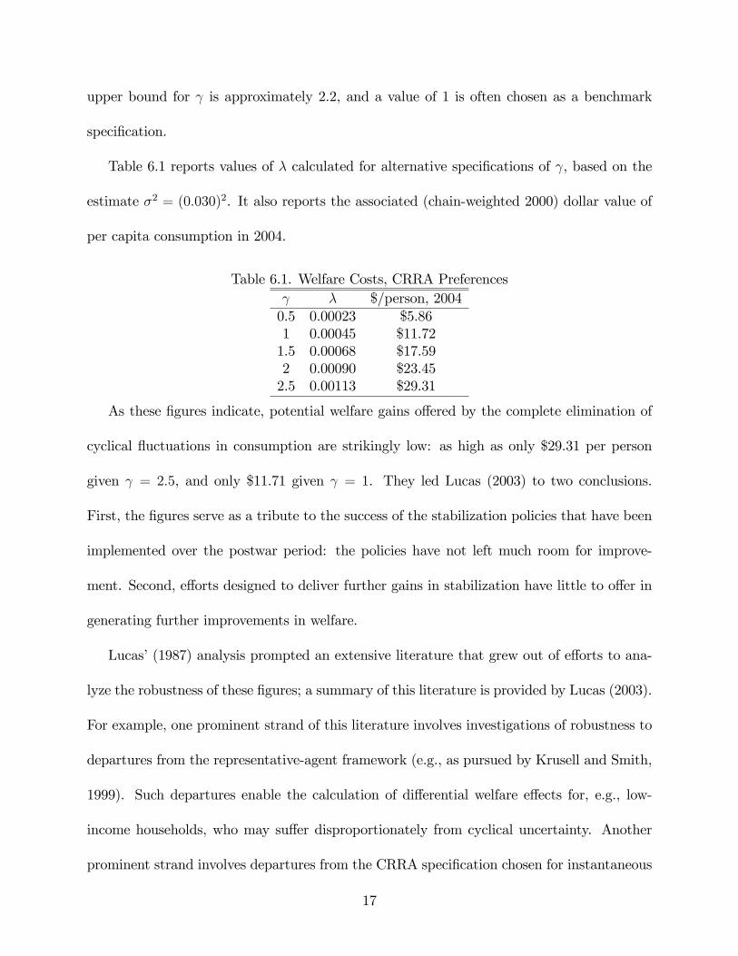
Table 6.1 reports values of � calculated for alternative speci�cations of , based on the

estimate �2 = (0:030)2. It also reports the associated (chain-weighted 2000) dollar value of

per capita consumption in 2004.

Table 6.1. Welfare Costs, CRRA Preferences � $/person, 20040.5 0.00023 $5.861 0.00045 $11.721.5 0.00068 $17.592 0.00090 $23.452.5 0.00113 $29.31

As these �gures indicate, potential welfare gains o¤ered by the complete elimination of

cyclical �uctuations in consumption are strikingly low: as high as only $29.31 per person

given = 2:5, and only $11.71 given = 1. They led Lucas (2003) to two conclusions.

First, the �gures serve as a tribute to the success of the stabilization policies that have been

implemented over the postwar period: the policies have not left much room for improve-

ment. Second, e¤orts designed to deliver further gains in stabilization have little to o¤er in

generating further improvements in welfare.

Lucas�(1987) analysis prompted an extensive literature that grew out of e¤orts to ana-

lyze the robustness of these �gures; a summary of this literature is provided by Lucas (2003).

For example, one prominent strand of this literature involves investigations of robustness to

departures from the representative-agent framework (e.g., as pursued by Krusell and Smith,

1999). Such departures enable the calculation of di¤erential welfare e¤ects for, e.g., low-

income households, who may su¤er disproportionately from cyclical uncertainty. Another

prominent strand involves departures from the CRRA speci�cation chosen for instantaneous

17

utility. Lucas� (2003) reading of this literature led him to conclude that his original cal-

culations have proven to be remarkably robust. Here we demonstrate an extension that

underscores this conclusion, adopted from Otrok (2001).

Otrok�s extension involves the replacement of the CRRA speci�cation for instantaneous

utility with the habit/durability speci�cation introduced in Chapter 5. Otrok�s analysis was

conducted in the context of a fully speci�ed RBC model featuring a labor/leisure trade-o¤,

along with a consumption/investment trade-o¤. The parameters of the model were estimated

using Bayesian methods discussed in Chapter 9. Here, we adopt Otrok�s estimates of the

habit/durability parameters in pursuit of calculations of � akin to those made by Lucas

(1987, 2003) for the CRRA case.

Recall that under habit/durability preferences, instantaneous utility is given by

u(ht) =h1� t

1� ; (14)

with

ht = hdt � �hht ; (15)

where � 2 (0; 1), hdt is the household�s durability stock, and hht its habit stock. The stocks

are de�ned by,

hdt =

1Xj=0

�jct�j (16)

hht = (1� �)1Xj=0

�jhdt�1�j = (1� �)1Xj=0

�j1Xi=0

�ict�1�i (17)

18

where � 2 (0; 1) and � 2 (0; 1). Substituting for hdt and hht in (15) thus yields

ht = ct +

1Xj=1

"�j � �(1� �)

j�1Xi=0

�i�j�i�1

#ct�j �

1Xj=0

�jct�j; (18)

where �0 � 1.

Combining (14) and (18) with (10), Lucas�welfare comparison in this case involves the

calculation of � such that

E0

1Xt=0

�t

"(1 + �)

(1Pj=0

�jct�j

)#1� 1� =

1Xt=0

�t

1Pj=0

�jAe�t�j

!1� 1� ; (19)

where once again the behavior of ct is given by (6). In this case, a convenient analytical

expression for � is unavailable, due to the complicated nature of the integral needed to

calculate the expectation on the left-hand-side of (19). Hence we proceed in this case by

approximating � numerically.

The algorithmwe employed for this purpose takes the collection of parameters that appear

in (19) and (6), including �, as given. The parameters (A; �; �2), dictating the behavior of

consumption, were obtained once again from an OLS regression of log ct on a constant and

trend; the parameters (�; ; �; �; �) were obtained from Otrok (2001), and a grid of values

was speci�ed for �. Since Otrok�s estimates were obtained using postwar quarterly data on

per capita consumption, de�ned as the consumption of non-durables and services, we re-

estimated (A; �; �2) using this alternative measure of consumption. The series is contained

in ycih.txt, available at the textbook website. It is slightly more volatile than the annual

measure of consumption considered by Lucas: the estimate of �2 it yields is (0:035)2.

19

Given a speci�cation of parameters, the right-hand-side of (19) may be calculated di-

rectly, subject to two approximations. First, for each value of t, the in�nite-order expression

1Pj=0

�jAe�t�j must be calculated using a �nite-ordered approximation. It turns out that under

the range of values for (�; ; �; �; �) estimated by Otrok, the corresponding sequence f�jg

decays rapidly as j increases, reaching approximately zero for j = 6; we set an upper bound

of J = 10 to be conservative. Second, the in�nite time horizon over which the discounted

value of instantaneous utility is aggregated must also be truncated. It turns out that sum-

mation over approximately a 1,500-period time span provides an accurate approximation of

the in�nite time horizon; we worked with an upper bound of T = 3; 000 to be conservative.

Using the same upper limits J and T , an additional approximation is required to calculate

the expectation that appears on the left-hand-side of (19). This is accomplished via use of a

technique known as numerical integration. Full details on the general use of this technique

are provided in Chapter 9. In the present application, the process begins by obtaining

a simulated realization of futgTt=1 from an N(0; �2) distribution, calculating f"tgTt=1 using

"t = eut, and then inserting f"tgTt=1 into (6) to obtain a simulated drawing of fctg

Tt=1. Using

this drawing, the corresponding realization of the discounted value of instantaneous utility is

calculated. These steps deliver the value of a single realization of lifetime utility. Computing

the average value of realized lifetime utilities calculated over many replications of this process

yields an approximation of the expected value of lifetime utility. The results reported below

were obtained using 1,000 replications of this process.5

Finally, to determine the value of � that satis�es (19), the left-hand-side of this equation

5A discussion of the accuracy with which this calculation approximates the actual integral we seek. isprovided in Chapter 9.

20

was approximated over a sequence of values speci�ed for �; the speci�c sequence we used

began at 0 and increased in increments of 0.000025. Given the risk aversion implied by

the habit/durability speci�cation, the left-hand-side of (19) is guaranteed to be less than

the right-hand-side given � = 0; and as � increases, the left-hand-side increases, ultimately

reaching the value of the right-hand-side. The value of � we seek in the approximation is

that which generates equality between the two sides.

Results of this exercise are reported in Table 6.2 for nine speci�cations of (�; ; �; �; �).

The �rst is referenced as a baseline: these correspond with median values of the marginal

posterior distributions Otrok calculated for each parameter: 0.9878, 0.7228, 0.446, 0.1533,

0.1299. Next, sensitivity to the speci�cation of is demonstrated by re-specifying �rst at

the 5% quantile value of its marginal posterior distribution, then at its 95% quantile value.

The remaining parameters were held �xed at their median values given the re-speci�cation

of . Sensitivity to the speci�cations of �; �; and � is demonstrated analogously. Finally, a

modi�cation of the baseline under which = 1 is reported, to facilitate a closer comparison

of Lucas�estimate of � obtained under CRRA preferences given = 1.

Table 6.2. Welfare Costs, Habit/Durability PreferencesParameterization � $/person, 2004

Baseline 0.000275 $7.15 = 0:5363 0.000225 $5.85 = 0:9471 0.000400 $10.40� = 0:0178 0.000375 $9.75� = 0:3039 0.000200 $5.20� = 0:2618 0.000275 $7.15� = 0:6133 0.000400 $10.40� = 0:0223 0.000425 $11.05� = 0:3428 0.000175 $4.55 = 1 0.000550 $14.30

Note: Baseline estimates are (�; ; �; �; �) = (0:9878; 0:7228; 0:446; 0:1533; 0:1299).

21

Under Otrok�s baseline parameterization, � is estimated as 0.00275. In terms of the

annual version of consumption considered by Lucas, this corresponds with a consumption

cost of $7.15/person in 2004. For the modi�cation of the baseline under which = 1, the

cost rises to $14.30/person, which slightly exceeds the cost of $11.72/person calculated using

CRRA preferences given = 1. The estimated value of � is most sensitive to changes

in �, which determines the persistence of the �ow of services from past consumption in

contributing to the durability stock. However, even in this case the range of estimates is

modest: $4.55/person given � = 0:3428; $11.05/person given � = 0:0223. These results serve

to demonstrate the general insensitivity of Lucas�results to this particular modi�cation of

the speci�cation of instantaneous utility; as characterized by Otrok: �... it is a result that

casts doubt that empirically plausible modi�cations to preferences alone could lead to large

costs of consumption volatility.�[p. 88]

Exercise 1 Recalculate the welfare cost of business cycles for the CRRA case given a relax-

ation of the log-Normality assumption for f"tg. Do so using the following steps.

1. Using the consumption data contained in weldat.txt, regress the log of consumption

on a constant and trend. Use the resulting parameter estimates to specify (A; �; �2) in

(6), and save the resulting residuals in the vector u.

2. Construct a simulated realization of fctgTt=0, T = 3; 000, by obtaining random drawings

(with replacement) of the individual elements of u. For each of the t drawings ut you

obtain, calculate "t = eut; then insert the resulting drawing f"tgTt=0 into (6) to obtain

fctgTt=0.

22

3. Using the drawing fctgTt=0, calculateTPt=0

�t [(1+�)ct]1�

1� using � = 0:96; = 0:5; 1; 1:5; 2

(recalling that for = 1; x1�

1� = ln(x)); and � = 0; 0:000025; ..., 0:0001.

4. Repeat Steps 2 and 3 1,000 times, and record the average values ofTPt=0

�t [(1+�)ct]1�

1� you

obtain as approximations of E0TPt=0

�t [(1+�)ct]1�

1� .

5. Calculate the right-hand-side of (10) using the estimates of A and � obtained in Step

1. Do so for each value of considered in Step 3.

6. For each value of , �nd the value of � that most closely satis�es (10). Compare the

values you obtain with those reported in Table 6.1. Are Lucas� original calculations

robust to departures from the log-Normality assumption adopted for f"tg?

Exercise 2 Using the baseline estimates of the habit/durability speci�cation reported in Ta-

ble 6.2, evaluate the robustness of the estimates of � reported in Table 6.2 to departures from

the log-Normality assumption adopted for f"tg. Do so using simulations of fctgTt=0 generated

as described in Step 2 of the previous exercise. Once again, are the results reported in Table

6.2 robust to departures from the log-Normality assumption adopted for f"tg?

4 Productivity Shocks and Business Cycle Fluctuations

As an example of an experiment involving a question of �t, we calibrate the RBC

model presented in Chapter 5.1, and examine the extent to which it is capable of accounting

for aspects of the behavior of output, consumption, investment and hours introduced in

Chapters 3 and 4 (the data are contained in ycih.txt, available at the textbook website).

Reverting to the notation employed in the speci�cation of the model, the parameters to be

23

calibrated are as follows: capital�s share of output �; the subjective discount factor � = 11+%;

where % is the subjective discount rate; the degree of relative risk aversion �; consumption�s

share (relative to leisure) of instantaneous utility '; the depreciation rate of physical capital

�; the AR parameter speci�ed for the productivity shock �; and the standard deviation of

innovations to the productivity shock �:

Standard speci�cations of � result from the association of the subjective discount rate

% with average real interest rates: roughly 4%-5% on an annual basis, or 1%-1.25% on a

quarterly basis. As a baseline, we select a rate of 1%, implying � = 11:01

= 0:99: The

parameterization of the CRRA parameter was discussed in the previous section; as a baseline,

we set � = 1:5; and consider [0:5 2:5] as a plausible range of alternative values.

We use the long-run relationship observed between output and investment to identify

plausible parameterizations of � and �: Recall that steady state values of ynand i

nare given

by

y

n= �;

i

n= ��;

where

� =

��

%+ �

� 11��

;

� = ��:

Combining these expressions yields the relationship

� =

�� + %

�

�i

y: (20)

24

Using the sample average of 0.175 as a measure of iy; and given % = 0:01; a simple relationship

is established between � and �:

Before illustrating this relationship explicitly, we use a similar step to identify a plausible

range of values for ': Here we employ the steady state expression for n; the fraction of

discretionary time spent on job-market activities:

n =1

1 +�

11��� �

1�''

� �1� ��1��

� : (21)

According to the time-allocation study of Ghez and Becker (1975), which is based on house-

hold survey data, n is approximately 1/3. Using this �gure in (21), and exploiting the

fact that cy=�1� ��1��

�(the sample average of which is 0.825), we obtain the following

relationship between � and ':

' =1

1 + 2(1��)c=y

: (22)

In sum, using sample averages to pin down iy; cy; and n; we obtain the relationships

between �; �; and ' characterized by (20) and (22). Table 6.3 presents combinations of

these parameters for a grid of values speci�ed for � over the range [0:01, 0:04] ; implying

a range of annual depreciation rates of [4%, 16%] : As a baseline, we specify � = 0:025

(10% annual depreciation), yielding speci�cations of � = 0:24 and ' = 0:35 that match

the empirical values of iy; cy; and n: Regarding the speci�cation of �; this is somewhat

lower than the residual value attributed to capital�s share given the measure of labor�s share

calculated from National Income and Product Accounts (NIPA) data. In the NIPA data,

labor�s share is approximately 2/3, implying the speci�cation of � = 1=3: The reason for the

25

di¤erence in this application is the particular measure of investment we employ (real gross

private domestic investment). Using the same measure of investment over the period 1948:I

- 1995:IV, DeJong and Ingram (2001) obtain an estimate of � = 0:23 (with a corresponding

estimate of � = 0:02) using Bayesian methods described in Chapter 9.

Table 6.3. Trade-O¤s Between �; � and ':� � '

0.010 0.35 0.390.015 0.29 0.370.020 0.26 0.360.025 0.24 0.350.030 0.23 0.350.035 0.22 0.350.040 0.22 0.35

Note: The moments used to establish these trade-o¤s areiy= 0:175; c

y= 0:825; and n = 1=3:

The �nal parameters to be established are those associated with the behavior of the

productivity shock zt: � and �:We obtain these by �rst measuring the behavior of zt implied

by the speci�cation of the production function, coupled with the observed behavior of output,

hours and physical capital. Given this measure, we then estimate the AR parameters directly

via OLS.

Regarding physical capital, the narrow de�nition of investment we employ must be taken

into account in measuring the corresponding behavior of capital. We do so using a tool

known as the perpetual inventory method. This involves the input of fitgTt=1 and k0 into the

law of motion of capital

kt+1 = it + (1� �)kt (23)

to obtain a corresponding sequence fktgTt=1 : A measure of k0 may be obtained in four steps:

divide both sides of (23) by yt; use beginning-of-sample averages to measure the resulting

26

ratios xy; x = i; k; solve for

k

y=1

�

i

y; (24)

and �nally, multiply 1�iyby y0: The results reported here are based on the speci�cation of iy

obtained using an eight-period, or two-year sample average.

Given this measure of fktgTt=1 ; log zt is derived following Solow (1957) as the unexplained

component of log yt given the input of log kt and log nt in the likelihood function:

log zt = log yt � � log kt � (1� �) log nt: (25)

For this reason, zt is often referred to as a Solow residual. Finally, we apply the Hodrick-

Prescott �lter to each variable, and estimate � and � using the HP-�ltered version of zt: The

resulting estimates are 0.78 and 0.0067.

Having parameterized the model, we characterize its implications regarding the collection

of moments reported for the HP-�ltered data in Table 4.1. Moments calculated using both

the model and data are reported in Table 6.4.

Table 6.4. Moment ComparisonH-P Filtered Data RBC Model

j �j�j�y

'(1) 'j;y(0) 'j;y(1) �j�j�y

'(1) 'j;y(0) 'j;y(1)

y 0.0177 1.00 0.86 1.00 0.86 0.0207 1.00 0.87 1.00 0.87c 0.0081 0.46 0.83 0.82 0.75 0.0101 0.48 0.94 0.96 0.93i 0.0748 4.23 0.79 0.95 0.80 0.0752 3.63 0.81 0.98 0.79n 0.0185 1.05 0.90 0.83 0.62 0.0076 0.366 0.78 0.97 0.76Notes: '(1) denotes �rst-order serial correlation; 'j;y(l) denotes l � th order

correlation between variables j and y: Model moments based on the parameterization� = [� � � ' � � �]0 = [0:24 0:99 1:5 0:35 0:025 0:78 0:0067]0:

As these results indicate, the model performs well in characterizing the patterns of serial

27

correlation observed in the data, and also replicates the patterns of volatility observed for

consumption and investment relative to hours: the former is quite smooth relative to the

latter. However, it performs poorly in characterizing the relative volatility of hours, which

are roughly equally as volatile as output in the data, but only 1/3 as volatile in the model.

Figure 6.1 illustrates this shortcoming by depicting the time-series paths followed by output

and hours in the actual data, along with paths followed by counterparts simulated from the

model. The simulated hours series is far smoother than the corresponding output series.

Figure 6.1. Comparisons of Output and Hours.

The standard RBC model�s characterization of the volatility of hours is a well-known

shortcoming, and has prompted many extensions that improve upon its performance along

this dimension. Examples include speci�cations featuring indivisible labor hours (Hansen,

28

1985; Rogerson, 1988; Kydland and Prescott, 1991b); home production (Benhabib, Rogerson,

and Wright, 1991; Greenwood and Hercowitz, 1991); labor hoarding (Burnside, Eichenbaum

and Rebelo, 1993; Burnside and Eichenbaum, 1997); �scal disturbances (McGrattan, 1994);

and skill-acquisition activities (Einarsson and Marquis, 1997; Perli and Sakellaris, 1998; and

DeJong and Ingram, 2001). Thus this example serves as a prime case study for the use

of calibration experiments as a means of facilitating the �... testing and development of

theory�, as advocated by Kydland and Prescott (1996, p. 70).

Exercise 3 Reconstruct Table 6.4 by employing the alternative combinations of values speci-

�ed for �; �; and ' listed in Table 6.3. Also, consider 0.5 and 2.5 as alternative speci�cations

of �: Are the results of Table 6.4 materially altered by any of the alternative choices you con-

sidered?

Exercise 4 Reconduct the calibration exercise of this section using the extension of the RBC

model outlined in Chapter 5, Section 1 that explicitly incorporates long-term growth. Pay

careful attention to the fact that equations (20) and (22), used to restrict the parameteriza-

tions of �; �; and '; will be altered given this extension. So too will be (24), which was used

to specify k0: Once again, are the results of Table 6.4 materially altered given this extension

of the model?

5 The Equity Premium Puzzle

The calibration experiment of Mehra and Prescott (1985) also serves as a prime case

study involving the testing and development of theory. The test they conducted sought to

29

determine whether the asset-pricing model presented in Chapter 5.3 is capable of charac-

terizing patterns of returns generated by relatively risky assets (equity) and riskless assets

(Treasury bills). The data they considered for this purpose consist of the annual real return

on the Standard and Poor�s 500 composite index; the annualized real return on Treasury

bills; and the growth rate of real per capita consumption on non-durables and services. The

time span of their data is 1889-1978; here we demonstrate a brief replication of their study

using data updated through 2004. The original data set is contained in mpepp.txt, and the

updated data set is contained in mpeppext.txt; both are available at the textbook website.

As characterized in Chapter 5.3, Mehra and Prescott�s statement of the equity premium

puzzle amounts to a presentation of the empirical incompatibility of the following equations,

derived in a two-asset environment:

�Etu0(ct+1)

u0(ct)rft+1 � 1 = 0 (26)

Etu0(ct+1)

u0(ct)

hret+1 � r

ft+1

i= 0; (27)

where rft+1 and ret+1 denote the gross returns associated with a risk-free and risky asset.

The di¤erence ret+1 � rft+1 is referred to as the equity premium. Sample averages (standard

deviations) of rft+1 and ret+1 are 0.8% (5.67%) and 6.98% (16.54%) in the data ending in

1978, and 1.11% (5.61%) and 7.48% (16.04%) in the data ending through 2004. Thus equity

returns are large and volatile relate to risk-free returns. The question is: can this pattern

of returns be reconciled with the attitudes towards risk embodied by the CRRA preference

speci�cation?

Given CRRA preferences, with representing the risk-aversion parameter, the equations

30

are given by

�Et

�ct+1ct

�� rft+1 � 1 = 0 (28)

Et

�ct+1ct

�� hret+1 � r

ft+1

i= 0: (29)

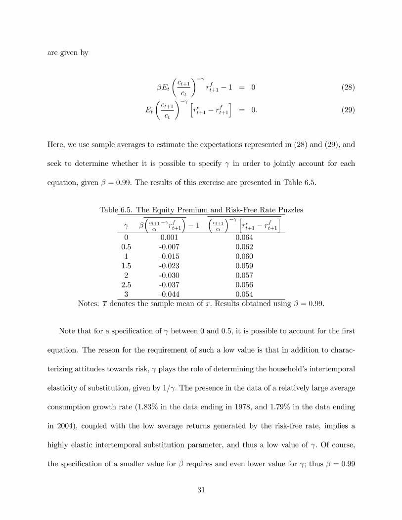
Here, we use sample averages to estimate the expectations represented in (28) and (29), and

seek to determine whether it is possible to specify in order to jointly account for each

equation, given � = 0:99: The results of this exercise are presented in Table 6.5.

Table 6.5. The Equity Premium and Risk-Free Rate Puzzles

��ct+1ct

� rft+1

�� 1

�ct+1ct

�� hret+1 � r

ft+1

i0 0.001 0.0640.5 -0.007 0.0621 -0.015 0.0601.5 -0.023 0.0592 -0.030 0.0572.5 -0.037 0.0563 -0.044 0.054

Notes: x denotes the sample mean of x: Results obtained using � = 0:99:

Note that for a speci�cation of between 0 and 0.5, it is possible to account for the �rst

equation. The reason for the requirement of such a low value is that in addition to charac-

terizing attitudes towards risk, plays the role of determining the household�s intertemporal

elasticity of substitution, given by 1= : The presence in the data of a relatively large average

consumption growth rate (1.83% in the data ending in 1978, and 1.79% in the data ending

in 2004), coupled with the low average returns generated by the risk-free rate, implies a

highly elastic intertemporal substitution parameter, and thus a low value of : Of course,

the speci�cation of a smaller value for � requires and even lower value for ; thus � = 0:99

31

represents nearly a best-case scenario along this dimension.

In turn, a large speci�cation of is required to account for the second equation. In

fact, the sample average �rst becomes negative given = 20: The reason for this is that

the relatively large premium associated with returns generated by the risky asset implies

substantial risk aversion on the part of households. This in turn implies a highly inelastic

intertemporal elasticity of substitution given CRRA preferences, which is inconsistent with

the �rst equation. Thus the puzzle.

Mehra and Prescott�s (1985) statement of the puzzle spawned an enormous literature

seeking to determine whether alterations of preferences or additional features of the envi-

ronment are capable of accounting for this behavior. Surveys of this literature are given by

Kocherlakota (1996) and Mehra and Prescott (2003). Certainly these e¤orts have served

to make headway towards a resolution; however the conclusion of both surveys is that the

equity premium remains a puzzle.

Exercise 5 Replicate the calculations presented in Table 6.5 using the baseline parameter-

ization of the habit/durability speci�cation presented in Section 6.3. Does this modi�cation

represent progress in resolving the puzzle? Ponder the intuition behind your �ndings.

6 Critiques and Extensions

6.1 Critiques

As noted, Kydland and Prescott�s (1982) use of a calibration exercise to implement the

DSGE model they studied represents a pathbreaking advance in the conduct of empirical

32

work in macroeconomic applications. Moreover, as illustrated in the applications above,

calibration exercises can certainly serve as an e¤ective means of making headway in empirical

applications involving general-equilibrium models. At a minimum, they are well-suited for

conveying a quick initial impression regarding the empirical strengths and weaknesses of

a given model along speci�c dimensions chosen by the researcher. This latter attribute is

particularly important, in that it provides an e¤ective means of discovering dimensions along

which extensions to the model are most likely to bear fruit.

This being said, the lack of statistical formality associated with calibration exercises

imposes distinct limitations upon what can be learned and communicated via their use.

Moreover, the particular approach advocated by Kydland and Prescott (as presented in

Section 2) for addressing empirical questions in the absence of a formal statistical framework

has been criticized on a variety of fronts. We conclude this chapter by summarizing certain

aspects of this criticism, and discussing some closely related extensions to calibration that

retain the general spirit of the exercise.

In the preface to his (1944) articulation of the probability approach to econometrics,

Haavelmo opened with a criticism of the approach that prevailed at the time. The criticism

is striking in its applicability to calibration exercises devoted to questions regarding �t:

So far, the common procedure has been, �rst to construct an economic the-

ory involving exact functional relationships, then to compare this theory with

some actual measurements, and, �nally, �to judge�whether the correspondence

is �good�or �bad.�Tools of statistical inference have been introduced, in some

degree, to support such judgements, e.g., the calculation of a few standard errors

33

and multiple-correlation coe¢ cients. The application of such simple �statistics�

has been considered legitimate, while, at the same time, the adoption of de�nite

probability models has been deemed a crime in economic research, a violation of

the very nature of economic data. That is to say, it has been considered legitimate

to use some of the tools developed in statistical theory without accepting the very

foundation upon which statistical theory is built. For no tool developed in the

theory of statistics has any meaning - except, perhaps, for descriptive purposes -

without being referred to some stochastic scheme. [p. iii]

Our interpretation of the thrust of this criticism is that in the absence of statistical

formality, communication regarding the results of an experiment is problematic. Judgements

of �good�or �bad.�, or as Kydland and Prescott (1996, p. 71) put it, judgements of whether

�... the predictions of theory match the observations...�, are necessarily subjective. In

applications such as Mehra and Prescott�s (1985) identi�cation of the equity premium puzzle,

empirical shortcomings are admittedly fairly self-evident. But in evaluating marginal gains in

empirical performance generated by various modi�cations of a baseline model, the availability

of coherent and objective reporting mechanisms is invaluable. No such mechanism is available

in conducting calibration exercises.

Reacting to Kydland and Prescott (1996), Sims (1996) makes a similar point:

Economists can do very little experimentation to produce crucial data. This

is particularly true of macroeconomics. Important policy questions demand opin-

ions from economic experts from month to month, regardless of whether profes-

sional consensus has emerged on the questions. As a result, economists normally

34

�nd themselves considering many theories and models with legitimate claims to

matching the data and predicting the e¤ects of policy. We have to deliver rec-

ommendations or accurate description of the nature of the uncertainty about the

consequences of alternative policies, despite the lack of a single accepted theory.

[p. 107]

Moreover:

Axiomatic arguments can produce the conclusion that anyone making deci-

sions under uncertainty must act as if that agent has a probability distribution

over the uncertainty, updating the probability distribution by Bayes�rule as new

evidence accumulates. People making decisions whose results depend on which of

a set of scienti�c theories is correct should therefore be interested in probabilistic

characterizations of the state of the evidence. [p. 108]

These observations lead him to conclude:

... formal statistical inference is not necessary when there is no need to choose

among competing theories among which the data do not distinguish decisively.

But if the data do not make the choice of theory obvious, and if decisions depend

on the choice, experts can report and discuss their conclusions reasonably only

using notions of probability. [p. 110]

Regarding the problem of choosing among given theories, there is no doubt that from a

classical hypothesis testing perspective, under which one model is posed as the null hypoth-

esis, this is complicated by the fact that the models in question are �necessarily false.�But

35

this problem is not unique to the analysis of DSGE models, as the epigram to this chapter

by Theil implies. Moreover, this problem is not an issue given the adoption of a Bayesian

perspective, under which model comparisons involve calculations of the relative probability

assigned to alternative models, conditional on the observed data. Under this perspective,

there is no need for the declaration of a null model; rather, all models are treated symmet-

rically, and none are assumed a priori to be �true.� Details regarding this approach are

provided in Chapter 9.

Also in reaction to Kydland and Prescott (1996), Hansen and Heckman (1996) o¤er

additional criticisms. For one, they challenge the view that calibration experiments involving

questions of �t are to be considered as distinct from estimation: �... the distinction drawn

between calibrating and estimating the parameters of a model is arti�cial at best.� [p. 91]

Their reasoning �ts nicely with the description provided in Section 1 of the means by which

the speci�cation of � is achieved via use of (4); and the means by which judgements of �t

are achieved via comparisons of �(fXtgTt=1) with �(�XMt

Tt=1):

Econometricians refer to the �rst stage as estimation and the second stage as

testing.... From this perspective, the Kydland-Prescott objection to mainstream

econometrics is simply a complaint about the use of certain loss functions for

describing the �t of a model to the data or for producing parameter estimates.

[p. 92]

In addition, Hansen and Heckman call into question the practice of importing parameter

estimates obtained from micro studies into macroeconomic models. They do so on two

grounds. First, such parameter estimates are associated with uncertainty. In part this

36

uncertainty can be conveyed by reporting corresponding standard errors, but in addition,

model uncertainty plays a substantial role (a point emphasized by Sims). Second, �... it is

only under very special circumstances that a micro parameter ... can be �plugged into�a

representative consumer model to produce an empirically concordant aggregate model.�[p.

88] As an example of such a pitfall, they cite Houthakker (1956), who demonstrated that

the aggregation of Leontief micro production technologies yields an aggregate Cobb-Douglas

production function.

These shortcomings lead Hansen and Heckman and Sims to similar conclusions. To quote

Hansen and Heckman:

Calibration should only be the starting point of an empirical analysis of

general-equilibrium models. In the absence of �rmly established estimates of

key parameters, sensitivity analyses should be routine in real business cycle sim-

ulations. Properly used and quali�ed simulation methods can be an important

source of information and an important stimulus to high-quality empirical eco-

nomic research. [p. 101]

And to quote Sims:

A focus on solving and calibrating models, rather than carefully �tting them

to data, is reasonable at a stage where solving the models is by itself a major

research task. When plausible theories have been advanced, though, and when

decisions depend on evaluating them, more systematic collection and comparison

of evidence cannot be avoided. [p. 109]

37

It is precisely in the spirit of these sentiments that we present the additional material

contained in Part II of this text.

6.2 Extensions

We conclude this chapter by presenting two extensions to the basic calibration exercise. In

contrast to the extensions presented in the chapters that follow, the extensions presented

here are distinct in that they do not entail an estimation stage. Instead, both are designed

to provide measures of �t for calibrated models.

The �rst extension is due to Watson (1996), who proposed a measure of �t based on

the size of the stochastic error necessary for reconciling discrepancies observed between the

second moments corresponding to the model under investigation and those corresponding

with the actual data. Speci�cally, letting Xt denote the m� 1 vector of observable variables

corresponding with the model, and Yt their empirical counterparts, Watson�s measure is

based on the question: how much error Ut would have to be added to Xt so that the

autocovariances of Xt + Ut are equal to the autocovariances of Yt?

To quantify this question, recall from Chapter 4 that the sth�order autocovariance of a

mean-zero covariance-stationary stochastic process zt is given by them�mmatrix Eztz0t�s �

�z(s): Therefore the sth�order autocovariance of Ut = Yt �Xt is given by

�U(s) = �Y (s) + �X(s)� �XY (s)� �Y X(s); (30)

where �XY (s) = EXtY0t�s; and �XY (s) = �Y X(�s)0: With the autocovariance generating

38

function ACGF of zt given by

Az(e�i!) =

1Xs=�1

�z(s)e�i!s; (31)

where i is complex and ! 2 [0; 2�] represents a particular frequency, the ACGF of Ut implied

by (30) is given by

AU(e�i!) = AY (e

�i!) + AX(e�i!)� AXY (e�i!)� AXY (ei!)0; (32)

where AXY (ei!)0 = AY X(e�i!):

As discussed in Chapter 4, it is straightforward to construct AY (e�i!) and AX(e�i!)

given observations on Yt and a model speci�ed for Xt: However, absent theoretical restric-

tions imposed upon AXY (e�i!); and absent joint observations on (Yt; Xt) ; the speci�cation

of AXY (e�i!) is arbitrary. Watson overcame this problem by proposing a restriction on

AXY (e�i!) that produces a lower bound for the variance of Ut; or in other words, a best-case

scenario for the model�s ability to account for the second moments of the data.

To characterize the restriction, it is useful to begin with the implausible but illustrative

case in which Xt and Yt are serially uncorrelated. In this case, the restriction involves

minimizing the size of the covariance matrix of Ut; given by

�U = �Y + �X � �XY � �Y X : (33)

As there is no unique measure of the size of �U ; Watson proposes the minimization of the

trace of W�U ; where W is an m�m weighting matrix that enables the researcher to assign

39

alternative importance to linear combinations of the variables under investigation. If W is

speci�ed as the identity matrix, then each individual variable is treated as equally important.

If alternatively the researcher is interested in GYt and GXt; then W can be chosen as G0G;

since tr(G�UG0) = tr(G0G�U):

Given W; Watson shows that

�XY = CXV U0C 0Y (34)

is the unique speci�cation of �XY that minimizes tr(W�U): In (34), CX and CY are arbitrary

m �m matrix square roots of �X and �Y (e.g., �X = CXC 0X ; an example of which is the

Cholesky decomposition), and the matrices U and V are obtained by computing the singular

value decomposition of C 0YWCX : Speci�cally, the singular value decomposition of C0YWCX

is given by

C 0YWCX = USV0; (35)

where U is an m�k orthonormal matrix (i.e., U 0U is the k�k identity matrix), S is a k�k

matrix, and V is a k � k orthonormal matrix.6

For the general case in which Xt and Yt are serially correlated, Watson�s minimization

objective translates directly from �XY to AXY (e�i!): Recall from Chapter 4 the relationship

between ACGFs and spectra; in the multivariate case of interest here, the relationship is

given by

sz(!) =

�1

2�

� 1Xs=�1

�z(s)e�i!s; ! 2 [��; �]: (36)

6In GAUSS, Cholesky decompositions may be obtained using the command chol, and singular valuedecompositions may be obtained using the command svd1.

40

With CX(!) now denoting the matrix square root of sX(!) calculated for a given speci�cation

of !; etc., the speci�cation of AXY (e�i!) that minimizes tr(W�U) is given by

AXY (e�i!) = CX(!)V (!)U

0(!)C 0Y (!); (37)

where U(!) and V (!) are as indicated in (35).

In this way, the behavior of the minimum-variance stochastic process Ut may be analyzed

on a frequency-by-frequency basis. As a summary of the overall performance of the model,

Watson proposes a relative mean square approximation error (RMSAE) statistic, analogous

to a lower bound on 1�R2 statistics in regression analyses (lower is better):

rj(!) =AU(e

�i!)jjAY (e�i!)jj

; (38)

where AU(e�i!)jj denotes the jth diagonal element of AU(e�i!):

As an illustration, Figure 6.2 closely follows Watson by demonstrating the application of

his procedure to the RBC model presented in Section 4, parameterized as indicated in Table

6.4. Following Watson, the �gure illustrates spectra corresponding to �rst di¤erences of

both the model variables and their empirical counterparts. This is done to better accentuate

behavior over business-cycle frequencies (i.e., frequencies between 1/40 and 1/6 cycles per

quarter). The data were also HP-�ltered, and W was speci�ed as the 4� 4 identity matrix.7

7Three GAUSS procedures were used to produce this �gure: modspec.prc; dataspec.prc; anderrspec.prc. All are available at the textbook website.

41

Figure 6.2. Decomposition of Spectra.

The striking aspect of this �gure is that the model fails to capture the spectral peaks

observed in the data over business-cycle frequencies. Given this failure, associated RM-

SAE statistics are decidedly anticlimactic. Nevertheless, RMSAEs calculated for output,

consumption, investment and hours over the [1=40; 1=6] frequency range are given by 0.18,

0.79, 0.15 and 0.66; thus the model�s characterization of consumption and hours over this

range is seen to be particularly poor.

Watson�s demonstration of the failure of the standard RBC model to produce spectral

peaks prompted several e¤orts devoted to determining whether plausible modi�cations of the

model are capable of improving empirical performance along this dimension. For example,

Wen (1998) obtained an a¢ rmative answer to this question by introducing two modi�cations:

42

an employment externality, under which the level of aggregate employment has an external

a¤ect on sectoral output; and the speci�cation of habit formation in the enjoyment of leisure

activities. So too did Otrok (2001), for the model (described in Section 3) he used to analyze

the welfare cost of business cycles. Thus the results of Figure 6.2 do not provide a general

characterization of the empirical performance of RBC models along this dimension.

The second extension is due to related work by Canova (1995) and DeJong, Ingram and

Whiteman (1996). Each study proposed the replacement of a single set of values speci�ed

over � with a prior distribution �(�): The distribution induced by �(�) over a collection

of empirical targets chosen by the researcher is then constructed and compared with a cor-

responding distribution calculated from the actual data. For example, the collection of

moments featured in Table 6.4 used to evaluate the RBC model presented in Section 4 rep-

resents a common choice of empirical targets. Reverting to the notation employed in Section

2, hereafter we represent the selected targets as :

The di¤erence between these studies lies in the empirical distributions over they employ.

DeJong et al. worked with posterior distributions over obtained from the speci�cation of a

vector autoregressive (VAR) model for the actual data; Canova worked with sampling distri-

butions. Methodologies available for calculating posterior distributions are not presented in

this text until Chapter 9, so details regarding the implementation of the extension proposed

by DeJong et al. are not provided here. Instead, we present an algorithm for calculating

sampling distributions over induced by a VAR speci�cation for the data, and thus for

implementing Canova�s measure of �t. This represents a specialization of the Monte Carlo

method presented in Section 2 of Chapter 4 as a means of approximating standard errors

numerically.

43

Using the notation of Chapter 4, let the VAR speci�ed for Xt be given by

Xt = �1Xt�1 +�2Xt�2 + :::+�pXt�p + "t; E"t"0t = �: (39)

The algorithm takes as inputs OLS estimates b�j; j = 1; :::; p; b�; estimated residuals fb"tg ;and the �rst p observations of Xt; which serve as starting values. Given these inputs, a

simulated drawing eXp+1 may be constructed by obtaining an arti�cial drawing e"p from a

given distribution, and evaluating the right-hand-side of (39) using fX1; X2; :::; Xp�1; Xpg

and e"p: Next, eXp+2 is constructed by obtaining a second drawing e"p+1, and evaluating right-hand-side of (39) using

nX2; X3; :::; Xp; eXp+1

oand e"p: Performing T replications of this

process yields an arti�cial drawingn eXt

o:8 For each of J replications of this process, a

collection of J estimates of is calculated; the resulting distribution of approximates the

sampling distribution we seek.

There are two common general methods for obtaining arti�cial drawings e"t: One methodinvolves a distributional assumption for f"tg ; parameterized by b�: For example, let bS denotethe Cholesky decomposition of b�: Then under the assumption of Normality for f"tg ; drawingse"t may be obtained using e"t = bSeu; where eu represents anm�1 vector of independent N(0; 1)random variables. Alternatively, e"t: may be obtained as a drawing (with replacement) fromthe collection of residuals fb"tg :Let the distribution obtained for the ith element of be given by S(i); and let [a; b]i

denote the range of values for i derived by subtracting and adding one standard deviation

8The in�uence of the initial observations fX1; X2; :::; Xp�1; Xpg may be reduced by obtaining T + T 0

drawings of eXt; and discarding the �rst T 0 drawings in constructing n eXto :

44

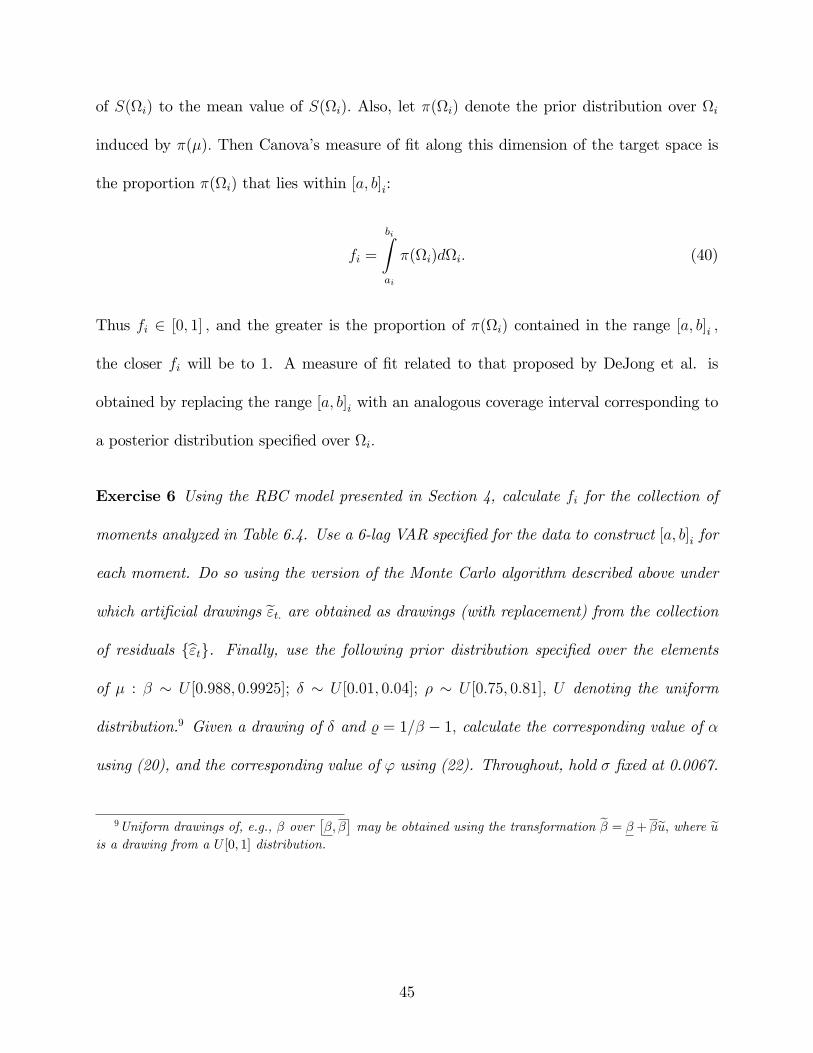
of S(i) to the mean value of S(i): Also, let �(i) denote the prior distribution over i

induced by �(�): Then Canova�s measure of �t along this dimension of the target space is

the proportion �(i) that lies within [a; b]i:

fi =

biZai

�(i)di: (40)

Thus fi 2 [0; 1] ; and the greater is the proportion of �(i) contained in the range [a; b]i ;

the closer fi will be to 1. A measure of �t related to that proposed by DeJong et al. is

obtained by replacing the range [a; b]i with an analogous coverage interval corresponding to

a posterior distribution speci�ed over i:

Exercise 6 Using the RBC model presented in Section 4, calculate fi for the collection of

moments analyzed in Table 6.4. Use a 6-lag VAR speci�ed for the data to construct [a; b]i for

each moment. Do so using the version of the Monte Carlo algorithm described above under

which arti�cial drawings e"t: are obtained as drawings (with replacement) from the collection

of residuals fb"tg. Finally, use the following prior distribution speci�ed over the elementsof � : � � U [0:988; 0:9925]; � � U [0:01; 0:04]; � � U [0:75; 0:81]; U denoting the uniform

distribution.9 Given a drawing of � and % = 1=� � 1; calculate the corresponding value of �

using (20), and the corresponding value of ' using (22). Throughout, hold � �xed at 0.0067.

9Uniform drawings of, e.g., � over��; �

�may be obtained using the transformation e� = � + �eu; where eu

is a drawing from a U [0; 1] distribution.

45

References

[1] Bank of Sweden. 1989. �Press Release: The Sveriges Riksbank (Bank of

Sweden) Prize in Economic Sciences in Memory of Alfred Nobel for 1989.�

http://nobelprize.org/economics/laureates/1989/press.html.

[2] Bank of Sweden. 2004. �Press Release: The Sveriges Riksbank (Bank of

Sweden) Prize in Economic Sciences in Memory of Alfred Nobel for 2004.�

http://nobelprize.org/economics/laureates/2004/press.html.

[3] Barro, R.J. and X. Sala-i-Martin. 2004. Economic Growth. 2nd Ed. Cambridge: MIT

Press.

[4] Benhabib, J. R. Rogerson and R. Wright. 1991. �Homework in Macroeconomics: House-

hold Production and Aggregate Fluctuations.�Journal of Political Economy 99:1166-

1187.

[5] Burnside, C. and M. Eichenbaum. 1997. �Factor-Hoarding and the Propagation of

Business-Cycle Shocks.�American Economic Review 86:1154-1174.

[6] Burnside, C., M. Eichenbaum and S. Rebelo. 1993. �Labor Hoarding and the Business

Cycle.�Journal of Political Economy 101:245-273.

[7] Canova, F. 1995. �Sensitivity Analysis and Model Evaluation in Simulated Dynamic

General Equilibrium Models.�International Economic Review 36:477-501.

46

[8] Cooley, T.F. and E.C. Prescott. 1995. �Economic Growth and Business Cycles.�in Fron-

tiers of Business Cycle Research, T.F. Cooley, Ed. 1-38. Princeton: Princeton University

Press.

[9] DeJong, D.N. and B.F. Ingram. 2001. �The Cyclical Behavior of Skill Acquisition.�

Review of Economic Dynamics 4:536-561.

[10] DeJong, D.N., B.F. Ingram and C.H. Whiteman. 1996. �A Bayesian Approach to Cali-

bration.�Journal of Business and Economic Statistics 14:1-9.

[11] Eichenbaum, M.S. 1983. �A Rational Expectations Equilibrium Model of Inventories of

Finished Goods and Employment.�Journal of Monetary Economics 12:71-96.

[12] Einarsson, T. and M.H. Marquis. 1997. �Home Production with Endogenous Growth.�

Journal of Monetary Economics 39:551-569.

[13] Frisch, R. 1933a. �Editorial.�Econometrica 1:1-5.

[14] Frisch, R. 1933b. �Propagation Problems and Impulse Problems in Dynamic Eco-

nomics.�In Economic Essays in Honor of Gustav Cassel. London.

[15] Frisch, R. 1970. �Econometrics in the World Today.�In Induction, Growth and Trade:

Essays in Honor of Sir Roy Harrod, W.A. Eltis, M.F.G. Scott, and J.N. Wolf, Eds.

152-166. Oxford: Clarendon Press.

[16] Greenwood, J. and Z. Hercowitz. 1991. �The Allocation of Capital and Time over the

Business Cycle.�Journal of Political Economy 99:1188-1214.

47

[17] Ghez, G.R. and G.S. Becker. 1975. The Allocation of Time and Goods over the Life

Cycle. New York: Columbia University Press.

[18] Haavelmo, T. 1944. �The Probability Approach in Econometrics.� Econometrica 12

(supplement):iii-vi and 1-115.

[19] Hansen, G.D. 1985. �Indivisible Labor and the Business Cycle.�Journal of Monetary

Economics 16:309-327.

[20] Hansen, L.P. and J.J. Heckman. 1996. �The Empirical Foundations of Calibration.�

Journal of Economic Perspectives 10:87-104.

[21] Hansen, L.P. and T.J. Sargent. 1980. �Formulating and Estimating Dynamic Linear

Rational Expectations Models.�Journal of Economic Dynamics and Control 2:7-46.

[22] Hansen, L.P. and T.J. Sargent. 1981. �Exact Linear Rational Expectations Models:

Speci�cation and Estimation.�Federal Reserve Bank of Minneapolis Sta¤ Report 71.

[23] Hansen, L.P. and K.J. Singleton. 1982. �Generalized Instumental Variables Estimation

of Nonlinear Rational Expectations Models.�Econometrica 50:1269-1286.

[24] Hansen, L.P. and K.J. Singleton. 1983. �Stochastic Consumption, Risk Aversion, and

the Temporal Behavior of Asset Prices.�Journal of Political Economy 91:249-265.

[25] Houthakker, H. 1956. �The Pareto Distribution and the Cobb-Douglas Production Func-

tion.�Review of Economic Studies 23:27-31.

[26] Kocherlakota, N. R. 1996. �The Equity Premium: It�s Still a Puzzle.�Journal of Eco-

nomic Perspectives XXXIV: 42-71.

48

[27] Koopmans, T.C. 1949. �The Econometric Approach to Business Fluctuations.�Ameri-

can Economic Review 39:64-72.

[28] Krusell, P. and A.A. Smith, Jr. 1999. �On the Welfare E¤ects of Eliminating Business

Cycles.�Review of Economic Dynamics 2:245-272.

[29] Kydland, F.E. and E.C. Prescott. 1982. �Time to Build and Aggregate Fluctuations.�

Econometrica 50: 1345-1370.

[30] Kydland, F.E. and E.C. Prescott. 1991a. �The Econometrics of the General Equilibrium

Approach to Business Cycles.�Scandinavian Journal of Economics 93:161-178.

[31] Kydland, F.E. and E.C. Prescott. 1991b. �Hours and Employment Variation in Business

Cycle Theory.�Economic Theory 1:63-81.

[32] Kydland, F.E. and E.C. Prescott. 1996. �The Computational Experiment: An Econo-

metric Tool.�Journal of Economic Perspectives 10:69-85.

[33] Lucas, R.E. 1978. �Asset Prices in an Exchange Economy.�Econometrica 46: 1429-1445.

[34] Lucas, R.E. 1980. �Methods and Problems in Business Cycle Theory.� Journal of

Money, Credit and Banking 12:696-715.

[35] Lucas, R.E. 1987. Models of Business Cycles. Oxford: Blackwell.

[36] Lucas, R.E. 2003. �Macroeconomic Priorities.�American Economic Review 93:1-14.

[37] Lundberg, E. 1969. Nobel Prize in Economics Presentation Speech.

http://nobelprize.org/economics/laureates/1969/press.html

49

[38] Mehra, R. and E.C. Prescott. 1985. �The Equity Premium: A Puzzle.� Journal of

Monetary Economics 15:145-161.

[39] Mehra, R. and E.C. Prescott. 2003. �The Equity Premium in Retrospect.�in Handbook

of the Economics of Finance, G.M. Constantinides, M. Harris and R. Stulz, Eds. 889-

936. Amsterdam: Elsevier.

[40] McGrattan, E. 1994. �The Macroeconomic E¤ects of Distortionary Taxation.�Journal

of Monetary Economics 94:573-601.

[41] Perli, R. and P. Sakellaris. 1998. �Human Capital Formation and Business Cycle Per-

sistence.�Journal of Monetary Economics 42:67-92.

[42] Otrok, C. 2001. �On Measuring the Welfare Cost of Business Cycles.�Journal of Mon-

etary Economics 47:61-92.

[43] Prescott, E.C. 1986. �Theory Ahead of Business Cycle Measurement.�Quarterly Re-

view, Federal Reserve Bank of Minneapolis 10:9-22.

[44] Rogerson, R. 1988. �Indivisible Labor, Lotteries and Equilibrium.�Journal of Monetary

Economics 21:3-16.

[45] Rowenhorst, G. 1991. �Time to Build and Aggregate Fluctuations: A Reconsideration,�

Journal of Monetary Economics 27: 241-254.

[46] Sargent, T.J. 1987. Macroeconomic Theory, 2nd Ed. London: Academic Press.

[47] Scarf, H. and T. Hansen. 1973. The Computation of Economic Equilibria. New Haven:

Yale University Press.

50

[48] Shoven, J.B. and J. Whalley. 1972. �A General Equilibrium Calculation of the E¤ects of

Di¤erential Taxation of Income from Capital in the U.S.�Journal of Public Economics

1:281-322.

[49] Sims, C.A. 1972. �Money, Income, and Causality.�American Economic Review 62:540-

552.

[50] Sims, C.A. 1996. �Macroeconomics and Methodology.�Journal of Economic Perspec-

tives 10:105-120.

[51] Solow, R.M. 1965. �A Contribution to the Theory of Economic Growth.�Quarterly

Journal of Economics 70:65-94.

[52] Theil, H. 1971. Principles of Econometrics. New York: Wiley.

[53] Watson, M. 1993. �Measures of Fit for Calibrated Models.�Journal of Political Economy

101:1011-1041.

51