STRATEGIC IMPLICATIONS OF US FIGHTER FORCE REDUCTIONS: …
84
STRATEGIC IMPLICATIONS OF US FIGHTER FORCE REDUCTIONS: AIR-TO-AIR COMBAT MODELING USING LANCHESTER EQUATIONS GRADUATE RESEARCH PAPER Ronald E. Gilbert, Major, USAF AFIT/IOA/ENS/11-01 DEPARTMENT OF THE AIR FORCE AIR UNIVERSITY AIR FORCE INSTITUTE OF TECHNOLOGY Wright-Patterson Air Force Base, Ohio APPROVED FOR PUBLIC RELEASE; DISTRIBUTION UNLIMITED
Transcript of STRATEGIC IMPLICATIONS OF US FIGHTER FORCE REDUCTIONS: …
STRATEGIC IMPLICATIONS OF US FIGHTER FORCE REDUCTIONS: AIR-TO-AIR COMBAT MODELING USING LANCHESTER EQUATIONS
GRADUATE RESEARCH PAPER
Ronald E. Gilbert, Major, USAF AFIT/IOA/ENS/11-01
DEPARTMENT OF THE AIR FORCE AIR UNIVERSITY
AIR FORCE INSTITUTE OF TECHNOLOGY
Wright-Patterson Air Force Base, Ohio
APPROVED FOR PUBLIC RELEASE; DISTRIBUTION UNLIMITED

The views expressed in this graduate research paper are those of the author and do not reflect the official policy or position of the United States Air Force, Department of Defense, or the United States government.
AFIT/IOA/ENS/11-01
STRATEGIC IMPLICATIONS OF US FIGHTER FORCE REDUCTIONS:
AIR-TO-AIR COMBAT MODELING USING LANCHESTER EQUATIONS
GRADUATE RESEARCH PAPER
Presented to the Faculty
Department of Operational Sciences
Graduate School of Engineering and Management
Air Force Institute of Technology
Air University
Air Education and Training Command
In Partial Fulfillment of the Requirements for the
Degree of Master of Science in Operational Analysis
Ronald E. Gilbert, BS, MBA
Major, USAF
June 2011
APPROVED FOR PUBLIC RELEASE; DISTRIBUTION UNLIMITED
AFIT/IOA/ENS/11-01
STRATEGIC IMPLICATIONS OF US FIGHTER FORCE REDUCTIONS: AIR-TO-AIR COMBAT MODELING USING LANCHESTER EQUATIONS
Ronald E. Gilbert, BS, MBA
Major, USAF
Approved: _____//SIGNED___________________________ 3 Jun 11 Dr John O. Miller, Civ, USAF (Advisor) Date
iv
AFIT/IOA/ENS/11-01
Abstract
Lanchester equations are used as the foundation for analysis of air superiority
forces, mathematically addressing the impending shortage of the United States fighters;
focusing on the role of advanced technology: stealth aircraft, air-to-air missiles, and the
rapid proliferation of electronic attack capabilities. These factors are accounted for in
determination of the attrition coefficients for heterogeneous fighter aircraft through a
simplistic scoring methodology and compared to potential adversarial states. ARENA
simulation is employed to determine minimal fighter requirements and expected blue
force losses as a function of threat force size and capability.
Analysis concludes that the United States is incapable of fighting a forward
deployed aerial battle against a numerically equal or superior force that employs
advanced technology unless initial force strength is at least half the adversarial totals. It
is recommended that the US leverage innovation and advance specific technological
areas surrounding fighter force lethality and survivability to address the deficiency in
aircraft numbers for the foreseeable future.
v
Table of Contents
Page
Abstract .............................................................................................................................. iv
List of Figures ................................................................................................................... vii
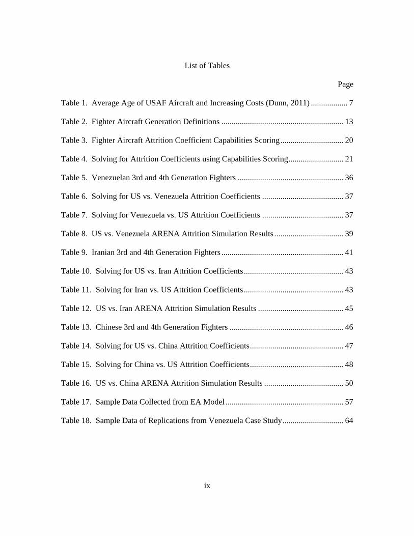
List of Tables ..................................................................................................................... ix
I. Introduction .....................................................................................................................1
Background...................................................................................................................1
Problem Statement........................................................................................................3
Previous Research ........................................................................................................4
Background Methodology ..........................................................................................11
II. Methodology ................................................................................................................16
ARENA Model – EA Effects .....................................................................................16
Running the EA Simulation........................................................................................16
ARENA Model – Lanchester Attrition .......................................................................17
Attrition Coefficient Determination ...........................................................................18
Initial Force Levels .....................................................................................................21
Maintenance Modeling ...............................................................................................21
Running the Attrition Simulation ...............................................................................23
III. Analysis and Results ...................................................................................................25
ARENA Model – EA Effects .....................................................................................25
ARENA Model – Lanchester Attrition .......................................................................27
Affects of Increasing Initial Fighter Numbers on Blue Losses ..................................28
Affects of Increasing Threat Numbers on Blue Losses ..............................................30
IV. Case Studies ................................................................................................................33
vi
Scenario Control .........................................................................................................33
Venezuela – Low Technology, Low Numbers ...........................................................36
IRAN – Moderate Technology, Moderate Numbers ..................................................40
China – High Technology, High Numbers .................................................................45
V. Conclusions and Recommendations .............................................................................52
Appendix A. List of Abbreviations and Acronyms ..........................................................56
Appendix B. Amplifying Data from ARENA Simulation Results ...................................57
Appendix C. Blue Dart…………………………………………………………………65
Bibliography ....................................................................................................................659
Vita ………………………………………………………………………………………72
vii
List of Figures
Page
Figure 1. US Aircraft Inventory Levels since 1950 (Ruehrmund and Bowie 2010:5) ...... 5
Figure 2. US Fighter Purchases per Year and Average Fighter Age (Grant 2009:21) ...... 6
Figure 3. Analysis Methodology...................................................................................... 12
Figure 4. Air Superiority Fighter Requirements to Kill 20 Threats ................................. 25
Figure 5. Missile Requirements as a Function of Missile Pk ........................................... 26
Figure 6. Blue Losses with Increasing EA for Varied Initial Force Strength .................. 28
Figure 7. Blue Losses at Varied EA and Increasing Initial Force Strength ..................... 29
Figure 8. Blue Losses with Increasing Threat Numbers for Varied Initial Fighters ........ 31
Figure 9. US Blue Losses vs. 100 3rd Gen and 100 4th Gen Chinese Fighters ................. 51
Figure 10. Blue Losses with Increasing EA for 12 F-15s and 6 F-22s ............................ 57
Figure 11. Blue Losses with Increasing EA for 16 F-15s and 8 F-22s ............................ 58
Figure 12. Blue Losses with Increasing EA for 20 F-15s and 10 F-22s .......................... 58
Figure 13. Blue Losses with Increasing EA for 24 F-15s and 12 F-22s .......................... 59
Figure 14. Blue Losses with No EA and Increasing Initial Force Strength ..................... 59
Figure 15. Blue Losses at 20% EA and Increasing Initial Force Strength ...................... 60
Figure 16. Blue Losses at 40% EA and Increasing Initial Force Strength ...................... 60
Figure 17. Blue Losses at 60% EA and Increasing Initial Force Strength ...................... 61
Figure 18. Blue Losses at 80% EA and Increasing Initial Force Strength ...................... 61
Figure 19. Blue Losses with Increasing Threat Numbers for 18 Initial Fighters ............ 62
Figure 20. Blue Losses with Increasing Threat Numbers for 24 Initial Fighters ............ 62
viii
Figure 21. Blue Losses with Increasing Threat Numbers for 30 Initial Fighters ............ 63
Figure 22. Blue Losses with Increasing Threat Numbers for 36 Initial Fighters ............ 63
ix
List of Tables
Page
Table 1. Average Age of USAF Aircraft and Increasing Costs (Dunn, 2011) .................. 7
Table 2. Fighter Aircraft Generation Definitions ............................................................ 13
Table 3. Fighter Aircraft Attrition Coefficient Capabilities Scoring ............................... 20
Table 4. Solving for Attrition Coefficients using Capabilities Scoring ........................... 21
Table 5. Venezuelan 3rd and 4th Generation Fighters .................................................... 36
Table 6. Solving for US vs. Venezuela Attrition Coefficients ........................................ 37
Table 7. Solving for Venezuela vs. US Attrition Coefficients ........................................ 37
Table 8. US vs. Venezuela ARENA Attrition Simulation Results .................................. 39
Table 9. Iranian 3rd and 4th Generation Fighters ............................................................ 41
Table 10. Solving for US vs. Iran Attrition Coefficients ................................................. 43
Table 11. Solving for Iran vs. US Attrition Coefficients ................................................. 43
Table 12. US vs. Iran ARENA Attrition Simulation Results .......................................... 45
Table 13. Chinese 3rd and 4th Generation Fighters ........................................................ 46
Table 14. Solving for US vs. China Attrition Coefficients .............................................. 47
Table 15. Solving for China vs. US Attrition Coefficients .............................................. 48
Table 16. US vs. China ARENA Attrition Simulation Results ....................................... 50
Table 17. Sample Data Collected from EA Model .......................................................... 57
Table 18. Sample Data of Replications from Venezuela Case Study .............................. 64
1
STRATEGIC IMPLICATIONS OF US FIGHTER FORCE REDUCTIONS: AIR-TO-AIR COMBAT MODELING USING LANCHESTER EQUATION
I. Introduction
Background
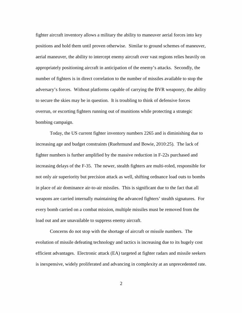
Over the past few decades, the United States military fought comfortably under a
blanket of air dominance. In the next few years, the small, almost unnoticeable hole in
that blanket grows considerably as its fighter aircraft force decreases, affecting the war-
fighters in the air and on the ground and bringing to question its ability to protect itself in
support of military policies abroad.
In World War II, the benefits of air dominance took a global stage; enabling the
ground forces and naval fleets to enact military might on their foes without regard. In the
conflicts since, this theme has been repeated and the importance of controlling the skies
has not been overlooked. In the most impressive demonstration of aerial dominance, the
coalition air forces of Desert Storm, led by the US Air Force shut down the Iraqi ability
to wage aerial warfare, guaranteeing the successful liberation of Kuwait. Victory was
delivered by the large US fighter inventory capable of finding enemy aircraft, engaging
them beyond visual range (BVR) and employing long range missiles, downing their
enemy with unmatched success.
In 1991, the US Air Force fighter inventory numbered 4155 (Ruehrmund and
Bowie, 2010:23). This number is significant for two reasons. First and foremost, a large
2
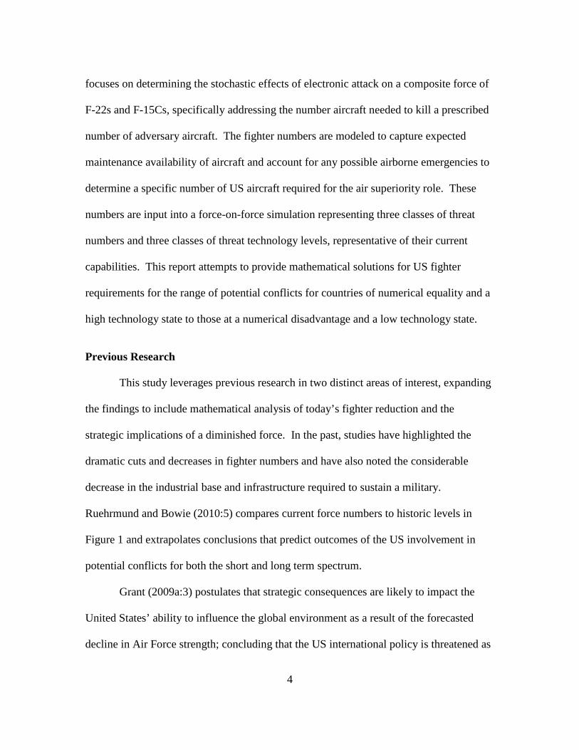
fighter aircraft inventory allows a military the ability to maneuver aerial forces into key
positions and hold them until proven otherwise. Similar to ground schemes of maneuver,
aerial maneuver, the ability to intercept enemy aircraft over vast regions relies heavily on
appropriately positioning aircraft in anticipation of the enemy’s attacks. Secondly, the
number of fighters is in direct correlation to the number of missiles available to stop the
adversary’s forces. Without platforms capable of carrying the BVR weaponry, the ability
to secure the skies may be in question. It is troubling to think of defensive forces
overrun, or escorting fighters running out of munitions while protecting a strategic
bombing campaign.
Today, the US current fighter inventory numbers 2265 and is diminishing due to
increasing age and budget constraints (Ruehrmund and Bowie, 2010:25). The lack of
fighter numbers is further amplified by the massive reduction in F-22s purchased and
increasing delays of the F-35. The newer, stealth fighters are multi-roled, responsible for
not only air superiority but precision attack as well, shifting ordnance load outs to bombs
in place of air dominance air-to-air missiles. This is significant due to the fact that all
weapons are carried internally maintaining the advanced fighters’ stealth signatures. For
every bomb carried on a combat mission, multiple missiles must be removed from the
load out and are unavailable to suppress enemy aircraft.
Concerns do not stop with the shortage of aircraft or missile numbers. The
evolution of missile defeating technology and tactics is increasing due to its hugely cost
efficient advantages. Electronic attack (EA) targeted at fighter radars and missile seekers
is inexpensive, widely proliferated and advancing in complexity at an unprecedented rate.

3
Unfortunately, the US is still employing the same family of missiles as it did during the
Gulf War, albeit carried on lesser numbers of aircraft.
Problem Statement
In the past few decades, the United States government quantified the level of risk
it is willing to accept in respect to conflict in the global environment as a function of the
numerical strength of the military forces. This level of risk is associated with the ability
to combat oppressive forces on two separate fronts, represented by a distinct division of
the logistical supply chain and the fighting services. Recently, the risk associated with
waging two regional conflicts not co-located increased to a point that is no longer
acceptable. The country’s leadership decided that the US could no longer support two
major wars; instead, the country’s military could only fight one large campaign and one
smaller, less involved situation. Although quantified by the rough size of the conflict, a
specific numerical understanding in respect to the exact force strength required is not
established.
Multiple studies have been performed attempting to quantify the state of the US
military, specifically air dominance fighters and the strategic implications associated with
the decline in numbers. Most research focuses on a specific threat nation or future threat
capability, however; none of these studies attempt to employ mathematical methods to
empirically solve for the numerical requirements of air-to-air fighters. It is possible to
model a benign aerial environment utilizing simulation to isolate certain effects of
evolving technology, capture the relevant data and use it as an input to determine the
attrition coefficients for a series of Lanchester differential equations. This research
4
focuses on determining the stochastic effects of electronic attack on a composite force of
F-22s and F-15Cs, specifically addressing the number aircraft needed to kill a prescribed
number of adversary aircraft. The fighter numbers are modeled to capture expected
maintenance availability of aircraft and account for any possible airborne emergencies to
determine a specific number of US aircraft required for the air superiority role. These
numbers are input into a force-on-force simulation representing three classes of threat
numbers and three classes of threat technology levels, representative of their current
capabilities. This report attempts to provide mathematical solutions for US fighter
requirements for the range of potential conflicts for countries of numerical equality and a
high technology state to those at a numerical disadvantage and a low technology state.
Previous Research
This study leverages previous research in two distinct areas of interest, expanding
the findings to include mathematical analysis of today’s fighter reduction and the
strategic implications of a diminished force. In the past, studies have highlighted the
dramatic cuts and decreases in fighter numbers and have also noted the considerable
decrease in the industrial base and infrastructure required to sustain a military.
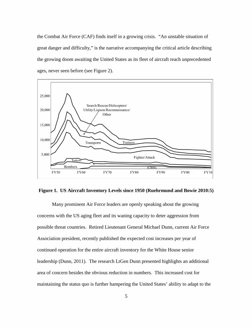
Ruehrmund and Bowie (2010:5) compares current force numbers to historic levels in
Figure 1 and extrapolates conclusions that predict outcomes of the US involvement in
potential conflicts for both the short and long term spectrum.
Grant (2009a:3) postulates that strategic consequences are likely to impact the
United States’ ability to influence the global environment as a result of the forecasted
decline in Air Force strength; concluding that the US international policy is threatened as
5
the Combat Air Force (CAF) finds itself in a growing crisis. “An unstable situation of
great danger and difficulty,” is the narrative accompanying the critical article describing
the growing doom awaiting the United States as its fleet of aircraft reach unprecedented
ages, never seen before (see Figure 2).
Figure 1. US Aircraft Inventory Levels since 1950 (Ruehrmund and Bowie 2010:5)
Many prominent Air Force leaders are openly speaking about the growing
concerns with the US aging fleet and its waning capacity to deter aggression from
possible threat countries. Retired Lieutenant General Michael Dunn, current Air Force
Association president, recently published the expected cost increases per year of
continued operation for the entire aircraft inventory for the White House senior
leadership (Dunn, 2011). The research LtGen Dunn presented highlights an additional
area of concern besides the obvious reduction in numbers. This increased cost for
maintaining the status quo is further hampering the United States’ ability to adapt to the

6
changing global climate and acquire newer, more advanced platforms. As stated by the
Under Secretary of Defense for Policy, Michele Flournoy, “the problem of aging
equipment is most acute for the Air Force…the service has been conducting combat
operations in the Gulf for the past 17 years, patrolling the desert skies. The same 17
years have seen underinvestment in modernization and recapitalization…a financial
burden that snowballs with every year,” (Dunn, 2011).
Figure 2. US Fighter Purchases per Year and Average Fighter Age (Grant 2009:21)
The previous Air Combat Command (ACC) commander, Retired General John
Corley, stresses the importance of a strong CAF, “USAF global tool sets are necessary to
underpin a national military or a national defense strategy, which, in turn, underpins a
national security strategy. Global power and global vigilance are where I would start as

7
we discuss the role of the CAF” (Laird, 2010:1). These comments are echoed by a series
of interviews and discussions led by Retired Lieutenant General David Deptula, the
former Air Force Chief of Intelligence, Surveillance and Reconnaissance. Most recently,
in September of last year, LtGen Deptula met with Defense Secretary Robert Gates and
exclaimed, “for the first time, our claim to air supremacy is in jeopardy,” further
exhorting, “the dominance we’ve enjoyed in the aerial domain is no longer ours for the
taking,” (Baron, 2010). His dreadful claims are reinforced by his research into the
emerging threat represented by multiple nation states, specifically addressing the leaps in
their technology and the US’ inability to maintain an equivalent pace (Deptula, 2010).
Table 1. Average Age of USAF Aircraft and Increasing Costs (Dunn, 2011)
Grant (2009b) argues that greater consequences exist for the extreme nature of the
fighter reduction, than those that appear readily on the surface of the discussion. Second
and third order effects are already being witnessed as defense organizations downsize

8
significantly or are forced to merge with other defense companies to maintain solvency.
These resultant business effects lead to a drop off in competition for government
contracts, which in turn diminishes technological innovation and ultimately decreases a
portion of the US’ military advantage. Although founded upon historical data, recent
trends, and expertise in the field of airpower, none of these studies quantify the scope of
the expected decrease in combat capability. Unfortunately, each of the previously
undertaken research endeavors lacks a mathematical foundation that elevates their
conclusions and recommendations beyond simplistic counting or rhetoric, to definitive,
quantifiable, areas of concern. Lastly, the USAF Chief of Staff, General Norton
Schwartz, remarked with regard to the change in the US’ assumed risk from “low” to
“moderate” as a consequence of the aging, decreasing fighter force, “the nature of risk is
that airmen will be unable, in a crisis, to successfully carry out their joint missions”
(Grant, 2009a:27).
Mathematically, combat analysis has been performed for thousands of years,
however; not since the early 1900’s have certain methods been understood or available
for utilization in military applications. In 1916, Frederick Lanchester developed a simple
series of differential equations that explain the relationship of two opposing forces and
their abilities to attrit the other over time (Lanchester, 1916: Ch 5). The Lanchester
Square Law Equations, listed below assume both forces use aimed fire (threat detected
and acquired) and the target acquisition time is independent of the number of targets.
9
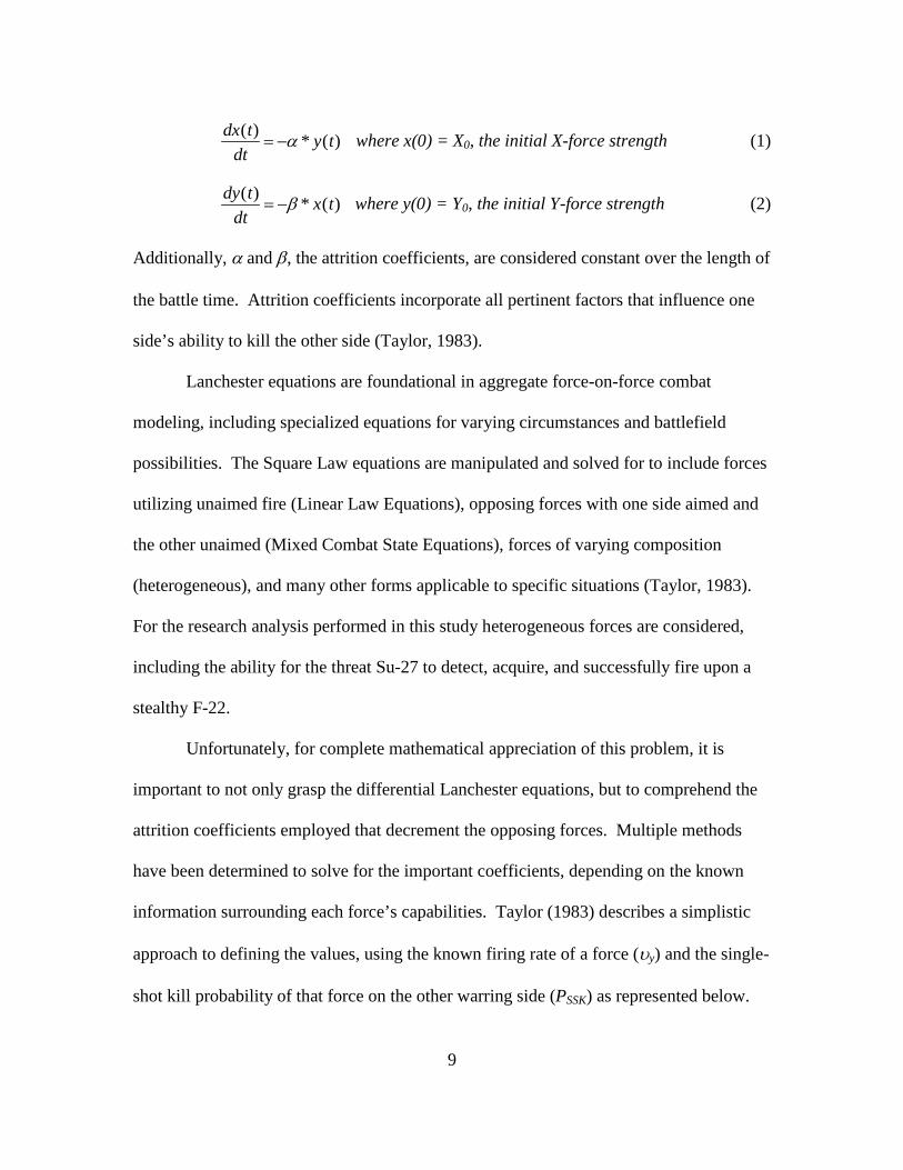
dx(t)dt
= −α * y(t) where x(0) = X0, the initial X-force strength (1)
dy(t)dt
= −β * x(t) where y(0) = Y0, the initial Y-force strength (2)
Additionally, α and β, the attrition coefficients, are considered constant over the length of
the battle time. Attrition coefficients incorporate all pertinent factors that influence one
side’s ability to kill the other side (Taylor, 1983).
Lanchester equations are foundational in aggregate force-on-force combat
modeling, including specialized equations for varying circumstances and battlefield
possibilities. The Square Law equations are manipulated and solved for to include forces
utilizing unaimed fire (Linear Law Equations), opposing forces with one side aimed and
the other unaimed (Mixed Combat State Equations), forces of varying composition
(heterogeneous), and many other forms applicable to specific situations (Taylor, 1983).
For the research analysis performed in this study heterogeneous forces are considered,
including the ability for the threat Su-27 to detect, acquire, and successfully fire upon a
stealthy F-22.
Unfortunately, for complete mathematical appreciation of this problem, it is
important to not only grasp the differential Lanchester equations, but to comprehend the
attrition coefficients employed that decrement the opposing forces. Multiple methods
have been determined to solve for the important coefficients, depending on the known
information surrounding each force’s capabilities. Taylor (1983) describes a simplistic
approach to defining the values, using the known firing rate of a force (υy) and the single-
shot kill probability of that force on the other warring side (PSSK) as represented below.

10
α = υ yPSSKXY (3)
Although this equation accounts for most simplistic models where each firing outcome is
statistically independent and the firing occurs at a uniform rate, it fails to account for
important aspects that are common in air combat. Bonder (1967) presents another
technique for determining attrition coefficients utilizing a single-shot Markov dependent
fire relationship. This equation uses known probabilities of success for each round fired
dependent on the success of previous shots. These probabilities are mathematically
combined in the equation below to determine the lethality (attrition coefficient) of one
force against another.
α =1
E[T]=
1ta
+1t1
−1th
+P(K | h)th + t f
+P(h | m)tm + t f
* P(K | h)1− P(h | h)
+1
P(h | h)−
1p1
(4)
Other methods exist for determining attrition coefficients such as the maximum
likelihood model that uses a time series of casualties to determine the mean time between
casualties and thus overall attrition rate (Clark, 1969).
Regrettably, none of these methods suffice when attempting to apply varying
technology and forces’ abilities to an attrition coefficient that accurately represents a
modern air force. Drew and others takes a different approach towards attrition
coefficients. The connection between own force survivability and the opposite forces’
attrition is associated. A probability of survival is determined, compared to the number
of sorties flown and used as the input to solve for an exchange ratio. This measure of
effectiveness describes the number of targets destroyed per own aircraft lost. Drew and
others further expands derivations to include factors that increase the probability of
survival, diminishing the adversary’s ability to attrit own forces. This process for

11
quantifying attrition coefficients is noteworthy; however, no closed form, easy to
replicate or adapt model is presented in their study.
Background Methodology
The approach to modeling the numerical requirements for military forces is not
new, however; the application of Lanchester equations to solve for air superiority fighter
numbers, explicitly addressing the role of technology is unique. In order to capture
relevant results that are of immediate benefit, the scope of the problem is limited. It is
anticipated that these results provide a launching point for future research capable of
attaining a greater level of depth, particularly related to quantifying other forms of
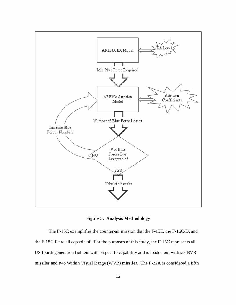
technology as it influences the attrition coefficients. ARENA simulation is employed to
model the effects of varying levels of EA on long-range missiles, setting the bounds on
numerical expectations in a benign scenario. The resultant data is entered into another
model that compares a hypothetical threat force with varied capabilities to determine the
probability of victory for the aerial battle. Once success is ensured (within criteria
discussed later) the US fighter force strength is varied to highlight the effect air
superiority numbers have on expected losses for a potential conflict (see Figure 3).
12
Figure 3. Analysis Methodology
The F-15C exemplifies the counter-air mission that the F-15E, the F-16C/D, and
the F-18C-F are all capable of. For the purposes of this study, the F-15C represents all
US fourth generation fighters with respect to capability and is loaded out with six BVR
missiles and two Within Visual Range (WVR) missiles. The F-22A is considered a fifth

13
generation fighter with obvious advantages of stealth technology, an advanced sensor
suite capable of fusing together multiple sources of battlefield information, and an
expanded envelope of flight operation up to 60,000ft and Mach 2.0. The load out for the
F-22 varies to characterize the different roles the aircraft is responsible for, however; for
this analysis the aircraft is equipped with six BVR and two WVR missiles. These
characteristics of fourth and fifth generation fighters are captured in the values for the
attrition coefficients.
Table 2. Fighter Aircraft Generation Definitions
Fighter Gen Era Capabilities Examples 1st Mid 1940s –Mid
1950s Initial Jet Engines,
Machine Gun Me 262, Meteor,
F-80, F-86, MiG-15 2nd Mid 1950s – Early
1960s Afterburner, bombs, RADAR, missiles
Mirage III, MiG-21, F-100, F-105, Su-7
3rd Early 1960s – 1970s Avionics, LGBs F-4, F-111, MiG-23 4th 1970s – Present HUD, HOTAS,
FLCS, Pulse-Doppler RADAR
F-15, F-16, F-18, MiG-29, Su-27,
Mirage 2000, J-10 5th 2005 - Present Stealth, Datalink,
Sensor Fusion, Advanced Avionics
F-22A, F-35, J-20, Su-PAK FA
The lone threat aircraft modeled in the initial analysis is the Su-27; however,
multiple 3rd and 4th generation aircraft are addressed and analyzed later in the case
studies. The Su-27 is widely sold to many countries worldwide and is an appropriate
representation of a capable foe in the air combat arena. Although its combination of
aircraft performance and avionics capabilities places it in the same class as the US fourth
generation fighters, the attrition coefficient assigned to the Su-27 is less than the F-15 due
to the minimal training and/or incomplete or non-existent tactical development that
14
international pilots receive on average. The BVR air-to-air missiles utilized by the Su-27
are shorter in range and less reliable than the US capability, further decreasing the
lethality of the Su-27 as a platform and impacting the corresponding attrition coefficient.
The scenario modeled begins with an initial number of aircraft from both forces
approaching the airspace of contention. There is no background information on a specific
threat country or its precise infrastructure of airfields and the geometry between them and
the fight. Instead arrival rates are handled as a constant, but may easily be manipulated
for application to a defined threat nation or Area of Responsibility (AOR). A significant
assumption associated with the entire scenario is that no air refueling is involved on
either side, with the exception of representing a forward location that reinforcement
fighters may arrive from. This eliminates discussion of aircraft cycling to and from the
tanker with varying ordnance and fuel states, dubbed beyond the scope of this
investigation. Additionally, both opposing forces are assumed to have access to a base
near the area of conflict that facilitates a base of operations and the potential for the
arrival of replacement forces as deemed appropriate.
A few important assumptions are made in regard to utilizing the Lanchester
differential equations. The mixed composition of F-15s and F-22s representing the
United States aerial capabilities typifies a heterogeneous force while the Su-27 threat is
simply representative of a homogeneous force. This is an important distinction due to
differing mathematical methods employed to handle each case. For this research,
Lanchester Square Law models for heterogeneous forces are used and simplified for the
Su-27 force. These equations are derived from a few assumptions of their own. The
15
most critical of these assumptions is that both sides use aimed fire. Although this may
seem obvious to most, it is necessary to describe the nature of BVR air-to-air missiles as
being RADAR guided, requiring detection and illumination of the targeted aircraft for a
valid weapon release. Other Lanchester equation assumptions are lumped into the
generality that nothing else is explicitly modeled; instead, the attrition coefficient
accounts for all other inputs collectively.

16
II. Methodology
ARENA Model – EA Effects
The first ARENA model was constructed with the intent to determine the number
of blue force aircraft, specifically BVR missiles, required to kill a given number of threat
aircraft operating with electronic attack targeted at the F-15 and F-22 composite force.
Quantifying the minimum number of missiles needed to attrit an opposing force provides
a lower bound for the problem of air superiority fighter requirements. Based on the
uncertainty of exact effects that a given EA environment might have, or exact effects
resulting from certain techniques, the rate of success for a missile launched against a non-
maneuvering, passive target was systematically varied to graphically depict the fighter
requirements over the range of potential. This graphical relationship holds true with any
software updates to the current BVR missile or the advent of a new missile in the future.
The basic scenario created resembles a common scenario flown in US training exercises
Red Flag Nellis, Red Flag Alaska, and the Dissimilar Air Combat Training (DACT)
portion of the USAF Weapons School syllabi. Twelve F-15Cs and six F-22s are posed
against an adversary force of twenty Su-27s. Although numerically representative, the
ARENA model lacks the tactical detail and specifics of actual air combat in order to
isolate the EA effects on the BVR missiles themselves.
Running the EA Simulation
The aircraft are created at time zero with no replacements planned. Each F-15
and F-22 begins with the standard conventional load-out (SCL) of six BVR missiles. The
targets (Su-27s) are assigned to available F-15s and F-22s. Each target is acquired
17
independently, allocated a missile and subsequently fired upon. For the EA model, no
threat maneuvers are simulated, no preference is given between F-15s and F-22s based on
current tactics to determine who would shoot, no counter-EA tactics or technology are
accounted for, and all missiles are assumed to be semi-active radar (SAR) guided with no
modeling of infrared (IR) seeker missiles. Each missile is assigned a probability of
success and compared to a random numerical draw to determine if it hits the assigned Su-
27. For every missile that hits a target it is assumed to be valid for a kill, eliminating the
target from the scenario. If the missile is determined to miss the target, the assigned
aircraft shoots another BVR missile and continues to do so until a kill is achieved. There
is no change in probability of success, even though theoretically the effects of EA are
reduced as the range between the fighter and the threat decrease. This process continues
until all 20 threats are destroyed or until all 18 blue force aircraft are out of BVR
missiles. This simulation is repeated ten times for each varied level of EA to account for
the variance between the random number draws for missile success. The output of the
EA model provides the average number of aircraft required for the given blue force
(twelve F-15s and six F-22s) to kill twenty threat aircraft for each of the incremented
levels of EA modeled. Time, aircraft fuel and aircraft system degradations amongst other
possibilities are not captured.
ARENA Model – Lanchester Attrition
The relationship between the EA environment and the number of aircraft needed
on average to kill a defined number of threats is input into the Lanchester attrition model
as an initial blue force number. Dependent upon the expected EA of a scenario, the
18
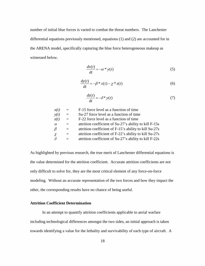
number of initial blue forces is varied to combat the threat numbers. The Lanchester
differential equations previously mentioned, equations (1) and (2) are accounted for in
the ARENA model, specifically capturing the blue force heterogeneous makeup as
witnessed below.
dx(t)dt
= −α * y(t)
(5)
dy(t)dt
= −β * x(t) − χ * z(t) (6)
dz(t)dt
= −δ * y(t)
(7)
x(t) = F-15 force level as a function of time y(t) = Su-27 force level as a function of time z(t) = F-22 force level as a function of time α = attrition coefficient of Su-27’s ability to kill F-15s β = attrition coefficient of F-15’s ability to kill Su-27s χ = attrition coefficient of F-22’s ability to kill Su-27s δ = attrition coefficient of Su-27’s ability to kill F-22s
As highlighted by previous research, the true merit of Lanchester differential equations is
the value determined for the attrition coefficient. Accurate attrition coefficients are not
only difficult to solve for, they are the most critical element of any force-on-force
modeling. Without an accurate representation of the two forces and how they impact the
other, the corresponding results have no chance of being useful.
Attrition Coefficient Determination
In an attempt to quantify attrition coefficients applicable to aerial warfare
including technological differences amongst the two sides, an initial approach is taken
towards identifying a value for the lethality and survivability of each type of aircraft. A
19
scorecard is created to solve for the value of the attrition coefficient with respect to each
type of combatant aircraft. The value is derived from the typical outcome observed at
Red Flag Nellis, Red Flag Alaska or the Weapons School DACT phase. These scenarios
on average result in 3-4 losses for 4th generation fighters and 1-2 losses for 5th generation
F-22s, with a decrease of 20-40% in missile Pk normally encountered. These reoccurring
exercise results, coupled with the author’s vast experience of over 1500 fighter hours in
the F-15C and F-22A and status as an Instructor in the Air Superiority Division of the
USAF Weapons School, 433rd Weapons Squadron, are foundational for the determination
of the attrition coefficient scoring.
The attrition coefficient is comprised of the advantages or disadvantages in
lethality directly compared to the opposing aircraft type and is awarded or deducted
points as appropriate. Each aircraft is given extra points, independent of the opposing
forces capabilities for technology related to survival: stealth and electronic attack. For
aircraft equipped with EA, the amount of points awarded varies with the techniques
employed that hinder the opposing forces ability to detect, acquire and/or target with a
BVR missile. For every 20% decrease in the opposing forces probability of kill (Pk) due
to EA, a greater increment of points is awarded. In addition to lethality and survivability,
a time constant (represented by points for both sides) is added to each aircraft to ensure
the fight is characterized accordingly with respect to the length of time expected for a
typical battle of the given proportions. Lastly, each aircraft receives a constant value for
their generational classification (3rd, 4th, 5th) based on their overall design and the era
introduced into service; ensuring each aircraft ends up with a coefficient greater than or

20
equal to zero. In the event an aircraft ends up with an attrition coefficient equal to zero, a
nominal value of 0.1 is used instead, to capture the rare possibility that the lesser foe is
able to find and kill the greater adversary by sheer chance. The following table outlines
the first attempt at providing structure to an otherwise ambiguous, difficult to define
measure for force-on-force modeling.
In the analysis, there are four attrition coefficients used in the differential
equations describing the ability of the F-15C to attrit the Su-27, the F-22’s ability to attrit
the Su-27 and the Su-27’s ability to attrit the F-15C and the F-22 independently. The
Lanchester equations modeled in this study, do not account for the synergistic effect of
the US composite force and is an area for recommended future research due to the
significant benefits of stealth and non-stealth fighter integration. Listed below is the
scorecard for each of the four separate comparisons and the resulting attrition
coefficients.
Table 3. Fighter Aircraft Attrition Coefficient Capabilities Scoring
21
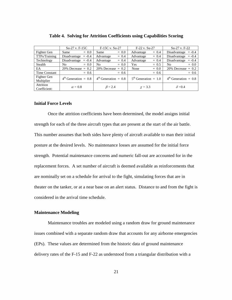
Table 4. Solving for Attrition Coefficients using Capabilities Scoring
Su-27 v. F-15C F-15C v. Su-27 F-22 v. Su-27 Su-27 v. F-22 Fighter Gen Same = 0.0 Same = 0.0 Advantage = 0.4 Disadvantage = -0.4 TTPs/Training Disadvantage = -0.4 Advantage = 0.4 Advantage = 0.4 Disadvantage = -0.4 Technology Disadvantage = -0.4 Advantage = 0.4 Advantage = 0.4 Disadvantage = -0.4 Stealth No = 0.0 No = 0.0 Yes = 0.5 No = 0.0 EA 20% Decrease = 0.2 20% Decrease = 0.2 None = 0.0 20% Decrease = 0.2 Time Constant = 0.6 = 0.6 = 0.6 = 0.6 Fighter Gen Multiplier 4th Generation = 0.8 4th Generation = 0.8 5th Generation = 1.0 4th Generation = 0.8
Attrition Coefficient: α = 0.8 β = 2.4 χ = 3.3 δ =0.4
Initial Force Levels
Once the attrition coefficients have been determined, the model assigns initial
strength for each of the three aircraft types that are present at the start of the air battle.
This number assumes that both sides have plenty of aircraft available to man their initial
posture at the desired levels. No maintenance losses are assumed for the initial force
strength. Potential maintenance concerns and numeric fall-out are accounted for in the
replacement forces. A set number of aircraft is deemed available as reinforcements that
are nominally set on a schedule for arrival to the fight, simulating forces that are in
theater on the tanker, or at a near base on an alert status. Distance to and from the fight is
considered in the arrival time schedule.
Maintenance Modeling
Maintenance troubles are modeled using a random draw for ground maintenance
issues combined with a separate random draw that accounts for any airborne emergencies
(EPs). These values are determined from the historic data of ground maintenance
delivery rates of the F-15 and F-22 as understood from a triangular distribution with a

22
minimum of 70% aircraft available, a maximum of 100% aircraft available and a mode of
90%. These values are combined with the historic values for airborne EPs uniformly
distributed between 1% and 8% to determine if an individual aircraft makes it into the
battle.
P(Fallout) = (1− TRIA(0.7,0.9,1))*UNIF(.01,.08)[ ]
The Su-27 force is decremented in similar fashion; however, due to the well-known
maintenance deficiencies abroad, the likelihood of both ground problems and airborne
issues are increased slightly, creating a greater chance that an aircraft may not make the
fight. Maintenance concerns for fighter aircraft manning is kept constant within the
statistical distributions mentioned; however, it is important to note two significant areas
not included in the analysis of this report. First, it is possible that aircraft maintenance
rates may decrease with time, due to obvious constraints faced in times of conflict and
any battle damage that occurs. Second, aircraft lost due to enemy actions are not
reflected. This has a significant impact on long-term sustainability of any force and
decreases aircraft availability of subsequent missions. Follow-on research is
recommended to capture time dependent aircraft availability rates in order to analyze in
greater detail the ability to preserve a fighting force over time. The average age of the
US’ fighter aircraft is a substantial concern as highlighted in the research mentioned
earlier. Maintenance modeling is captured in the arrival of reinforcements only not the
initial forces, due to the expectation that prepared spare aircraft would be available for
the initial fight.

23
Running the Attrition Simulation
The simulation begins with the initial number of aircraft input directly from the
EA ARENA model and steps through the Lanchester equations incrementally as time
progresses, constantly determining the current force levels, based on the rate of attrition
caused by the opposing force. Attrition continues for both forces until the first
reinforcements arrive into the aerial battle. The arrival aircraft immediately supplement
the appropriate force, increasing the rate of attrition of the opposite side. The air-to-air
fight continues until the termination criterion is met. The simulation ceases when either
force reaches zero aircraft remaining. The ARENA attrition simulation is run ten times
for each scenario to account for the variance in the maintenance production of aircraft for
the reinforcements of both sides. This provides an average number of aircraft lost for the
blue forces given a defined EA level and number of threats. The losses are compared to a
theoretical value for what is deemed acceptable by US senior leadership based on their
policies, as a given percentage of initial force strength. The simulation is repeated again,
varying the levels that leadership might accept to lose, solving for the forces required to
attain that desired outcome. Finally, the numbers are tabulated for analysis.
In the event, the F-15s and F-22s are destroyed first; the initial numbers are
incremented by four F-15s and two F-22s until a winning outcome is achieved. This ratio
between the blue fighters is maintained in order to capture the actual tactical formations
and employment standards currently trained to and expected to be utilized in the next

24
conflict. This allows the results to be compiled and compared to the current Air Force F-
15 and F-22 squadron strength giving insight into how many squadrons might be required
for certain threat countries.
25
III. Analysis and Results
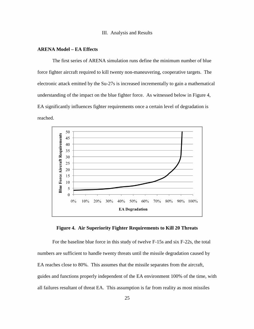
ARENA Model – EA Effects
The first series of ARENA simulation runs define the minimum number of blue
force fighter aircraft required to kill twenty non-maneuvering, cooperative targets. The
electronic attack emitted by the Su-27s is increased incrementally to gain a mathematical
understanding of the impact on the blue fighter force. As witnessed below in Figure 4,
EA significantly influences fighter requirements once a certain level of degradation is
reached.
Figure 4. Air Superiority Fighter Requirements to Kill 20 Threats
For the baseline blue force in this study of twelve F-15s and six F-22s, the total
numbers are sufficient to handle twenty threats until the missile degradation caused by
EA reaches close to 80%. This assumes that the missile separates from the aircraft,
guides and functions properly independent of the EA environment 100% of the time, with
all failures resultant of threat EA. This assumption is far from reality as most missiles
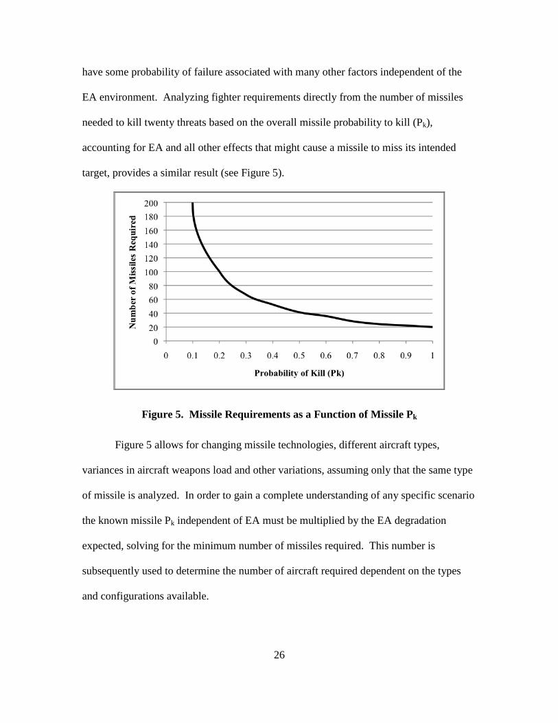
26
have some probability of failure associated with many other factors independent of the
EA environment. Analyzing fighter requirements directly from the number of missiles
needed to kill twenty threats based on the overall missile probability to kill (Pk),
accounting for EA and all other effects that might cause a missile to miss its intended
target, provides a similar result (see Figure 5).
Figure 5. Missile Requirements as a Function of Missile Pk
Figure 5 allows for changing missile technologies, different aircraft types,
variances in aircraft weapons load and other variations, assuming only that the same type
of missile is analyzed. In order to gain a complete understanding of any specific scenario
the known missile Pk independent of EA must be multiplied by the EA degradation
expected, solving for the minimum number of missiles required. This number is
subsequently used to determine the number of aircraft required dependent on the types
and configurations available.

27
ARENA Model – Lanchester Attrition
Lanchester differential equations are employed to determine the outcome of the
two opposing forces, specifically accounting for the technology, tactics, EA and stealth
capabilities of each side. The attrition coefficients are solved for using the scoring
method previously discussed and iterated for the varying levels of threat EA carried on
the Su-27. The ARENA attrition simulation runs begin with the baseline aircraft
numbers as output by the EA model (twelve F-15s, six F-22s and twenty Su-27s) with no
electronic attack to determine the total blue force losses.
Affects of Increasing EA on Blue Losses
As witnessed in Figure 6, expected blue force losses increase as the EA
degradation increases. Of note, there is an appreciable change in the rate of blue losses
between 40-50% EA degradation. Additionally, the total losses equal 18 aircraft at 80%
EA degradation, representing total blue force annihilation with the baseline initial
numbers. Improving the F-15 and F-22 initial force numbers helps lessen the blue force
losses as expected. The initial fighter numbers are augmented by four F-15s and two F-
22s to decrease the number of total losses by half at an EA degradation level of 80%.
This demonstrates the significance of initial force numbers on the total blue losses in an
EA environment. Further increases in the initial force strength amplify this result even
greater.
The blue losses continue to decrease with each additional four F-15s and two F-
22s added to the initial forces. Unfortunately, the decrease is only by two fighters each
time an additional six fighters are added. It appears that there is a marginal return for
initial numbers of the blue fighter force with respect to the initial threat force numbers.

28
Tactically, the more assets added, the more difficult it becomes to battle manage the fight
and deconflict aircraft; ensuring separation of forces and preventing friendly-fire
incidents from occurring. In the planning leading up to a campaign, an assessment
should be made on the opposing forces EA capabilities that in turn drive the theater level
fighter requirements. Once the EA level of the threat is known, an analysis on force
requirements is conducted, comparing the advantages of increasing the force posture and
the associated cost with doing so.
Figure 6. Blue Losses with Increasing EA for Varied Initial Force Strength
Affects of Increasing Initial Fighter Numbers on Blue Losses
In order to capture the exact effect of initial fighter strength, the threat EA is held
constant as the initial fighter numbers are increased from the baseline of 18 aircraft to 36
aircraft (24 F-15s and 12 F-22s) representative of two F-15 squadrons and one F-22
squadron on a typical deployment. Figure 7 below highlights the decreased risk of an
aerial battle with greater numbers present at the start of the fight.
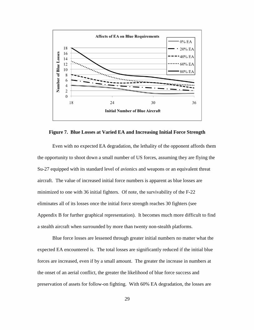
29
Figure 7. Blue Losses at Varied EA and Increasing Initial Force Strength
Even with no expected EA degradation, the lethality of the opponent affords them
the opportunity to shoot down a small number of US forces, assuming they are flying the
Su-27 equipped with its standard level of avionics and weapons or an equivalent threat
aircraft. The value of increased initial force numbers is apparent as blue losses are
minimized to one with 36 initial fighters. Of note, the survivability of the F-22
eliminates all of its losses once the initial force strength reaches 30 fighters (see
Appendix B for further graphical representation). It becomes much more difficult to find
a stealth aircraft when surrounded by more than twenty non-stealth platforms.
Blue force losses are lessened through greater initial numbers no matter what the
expected EA encountered is. The total losses are significantly reduced if the initial blue
forces are increased, even if by a small amount. The greater the increase in numbers at
the onset of an aerial conflict, the greater the likelihood of blue force success and
preservation of assets for follow-on fighting. With 60% EA degradation, the losses are

30
significant at the baseline force number of 18. An appreciable jump in losses occurs from
40-60% EA, as previously mentioned. This is quantified by 13 total blue force losses, an
increase from eight; however, the losses are reduced in half if the initial force numbers
are increased to at least 24. This drastic change is characterized by the curve of total blue
losses above, specifically the greater slope of the line initially.
At 80% EA total destruction of blue forces is witnessed with the baseline
numbers. Once again, an appreciable change in the blue losses is recognized once the
initial numbers are increased to 24. This inflection in the curve is important to identify in
force analysis and may provide the critical insight that dictates a minimum number of
forces required to combat a given adversary with a certain technological state
accompanying their numeric potential. This characteristic quantifies a specific ratio of
blue initial force fighters to the initial number of threat fighters and is important to
capture from simulation with respect to each side’s capabilities or more generally their
fighter generation comparisons (5th vs. 4th, 4th vs. 4th etc). From the attrition simulations,
it is possible to begin drawing conclusions; however, it is important to note that the threat
numbers are held constant thus far.
Affects of Increasing Threat Numbers on Blue Losses
Increasing threat numbers with moderate to high levels of EA creates a challenge
for any force to counter. Initial numbers must be equal if not greater than the opposing
force and other technological advantages must offset the effects presented by EA.
In Figure 8, the total number of threat aircraft is varied until the point of total blue force
destruction to determine if there is a critical point for the blue-to-red ratio with respect to

31
a given EA level. Eighteen total blue fighters (12+6) with no degradation to EA are used
as the baseline for comparison. As the threat numbers approach 30, an appreciable
increase in blue fighter attrition is noticed. Total destruction of the eighteen fighters
occurs at 35 threat aircraft.
Figure 8. Blue Losses with Increasing Threat Numbers for Varied Initial Fighters
The same simulation is run again, this time increasing the blue force initial
posture to 24 fighters. The output data shifts the blue losses significantly as expected,
this time with a noticeable increase in blue losses occurring at 35 threat aircraft and total
destruction of blue forces at 50 threat aircraft. Each increase in the initial blue fighter
strength produces similar results, with an identifiable bend in the curve each time as
previously discussed.
Analyzing the same scenario with 30 initial blue fighters (20 F-15s and 10 F-22s)
produces a less noticeable increase in blue fighter attrition around 50 threat aircraft.
Total destruction takes place at 60 total threat fighters. For 36 initial blue fighters, the

32
increased attrition point happens around 60 threat fighters with complete blue losses at 70
threats. Two trends in the data are identified when comparing the increasing number of
blue fighters and the resultant number of threats capable of being handled. It is apparent
that for this scenario, every increment in the initial force of blue fighters by four F-15s
and two F-22s delays the characteristic bend in the curve by ten threat aircraft, thus
delaying the point of increased attrition. Additionally, it is easily identifiable that total
destruction of blue forces occurs at roughly double their initial strength. This graphical
relationship may be constructed for any given scenario to capture the critical point in
attrition rates and quantifiably assess blue force requirements for any conflict. Although
simplistic in nature, it is important to ensure all variables (EA, tactics, training,
technology, generational classification of aircraft, as represented by the attrition
coefficient) are identified correctly to construct these charts and gain insight on these
important correlations.

33
IV. Case Studies
Scenario Control
With any assessment of a country’s military, it is important to concede that
numerical representation of their force strength is dynamic and is interpreted as a rough
approximation of their capabilities in two varied fashions. First, it is recognized that
some countries possess the capability to produce aircraft indigenously and true
operational numbers are difficult to capture. Secondly and of much greater significance
for analysis of any country, the exact understanding of a military’s capability to maintain
their aircraft in working order is often difficult to assess. These two areas for potential
force disparity should be addressed in any scenario. It is also appropriate to state that all
information gained for this analysis comes from open-source publications, void of all
classified intelligence channels in order to preserve the distribution of academic material
and spawn greater interest in this area of study.
Analyzing a specific country using Lanchester differential equations is difficult to
do based on the heavy assumptions required to facilitate the aerial battle. Assumptions
on the varied capabilities of the aircraft presented for each of the three countries below
must be simplified to produce results compatible with the research presented previously
in this analysis. All of the 4th generation fighters per country are considered equal and
are added together to produce a single representative number. The same approach is
taken for the 3rd generation fighters, lumping them together in order to have two separate
numbers representing a simplistic heterogeneous force for each country. The Lanchester
equations (5), (6), and (7) derived earlier for the generic scenario must be updated in the
34
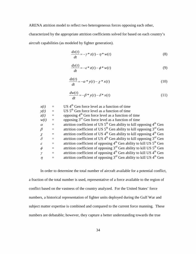
ARENA attrition model to reflect two heterogeneous forces opposing each other,
characterized by the appropriate attrition coefficients solved for based on each country’s
aircraft capabilities (as modeled by fighter generation).
dx(t)dt
= −γ * z(t) −η * w(t)
(8)
dy(t)dt
= −ε * z(t) − φ * w(t) (9)
dz(t)dt
= −α * y(t) − χ * x(t)
(10)
dw(t)dt
= −β * y(t) −δ * x(t)
(11)
x(t) = US 4th Gen force level as a function of time y(t) = US 5th Gen force level as a function of time z(t) = opposing 4th Gen force level as a function of time w(t) = opposing 3rd Gen force level as a function of time α = attrition coefficient of US 5th Gen ability to kill opposing 4th Gen β = attrition coefficient of US 5th Gen ability to kill opposing 3rd Gen χ = attrition coefficient of US 4th Gen ability to kill opposing 4th Gen δ = attrition coefficient of US 4th Gen ability to kill opposing 3rd Gen ε = attrition coefficient of opposing 4th Gen ability to kill US 5th Gen φ = attrition coefficient of opposing 3rd Gen ability to kill US 5th Gen γ = attrition coefficient of opposing 4th Gen ability to kill US 4th Gen η = attrition coefficient of opposing 3rd Gen ability to kill US 4th Gen
In order to determine the total number of aircraft available for a potential conflict,
a fraction of the total number is used, representative of a force available to the region of
conflict based on the vastness of the country analyzed. For the United States’ force
numbers, a historical representation of fighter units deployed during the Gulf War and
subject matter expertise is combined and compared to the current force manning. These
numbers are debatable; however, they capture a better understanding towards the true

35
outcome of force-on-force conflict between two countries, than the total assets.
Reinforcements are scheduled similarly, based on the proximity to the perceived battle
area and the location to the closest supporting bases or areas for tanker operations.
Military planning expertise is used to determine the specifics of aircraft that are dedicated
to the initial forces versus reinforcements that are scheduled to arrive from the tanker
refueling area. Maintenance modeling is applied as discussed earlier through ten total
replications of each case study scenario. The final results tabulated are averages from the
multiple replications (see Appendix B for sample data compiled).
The most important take away from this section is not the specifics or the
assumptions associated with the given AORs, but the comparison of an adversary with
low fighter numbers and minimal technology, a potential foe of moderate numbers and
average technology and a country of significant numbers and near-peer capabilities, to
the United States. The case studies are not intended for future planning in any of these
three areas; instead, they are intended to show application of a mathematical
methodology towards an initial understanding on conflict outcome. Military planners
with up-to-date intelligence coupled with the assistance of mathematical analysts have
the greatest insight into the potential force strengths of the two opposing sides, the
reinforcement expectations, the location and regional impacts as well as expected blue
force losses. Motivation or strategic reasoning for these conflicts is not discussed and is
considered beyond the scope of this analysis.

36
Venezuela – Low Technology, Low Numbers
The National Armed Forces of the Bolivian Republic of Venezuela are an ideal
representation of a smaller country’s military taking efforts to establish itself on the
global scene as a regional power, attempting to gain respect. Over the past five years, the
government took the first steps towards building a credible air defense by purchasing 24
advanced fighter aircraft. In addition to the newly acquired fighters, Venezuela is in
ongoing negotiations with Russia to purchase advanced surface-to-air-missile (SAM)
systems, further attempting to fortify their defenses. Although Venezuela represents
minimal threat to the sovereign United States proper, their anti-American rhetoric is
growing, as is their strategic alliance with Iran, bringing to question the future potential
for conflict in the area. Listed below are their 3rd and 4th generation aircraft deemed
operational at the current time.
Table 5. Venezuelan 3rd and 4th Generation Fighters
Aircraft Type / Generation Number Comparable to: Su-30MKV – 4th Gen 24 F-15E
F-16 – 4th Gen 20 F-16 CF-5 – 3rd Gen 16 F-5
Total: 60
Besides the basic technology that was included on their aircraft platforms,
Venezuela does not expand its aircraft lethality or survivability with additional
equipment. Most of their military modernization and technological investment, outside
of the basic equipped air defenses as mentioned, benefits their Army, including updated
personnel carriers, tanks, sniper rifles, night vision goggles and top-of-the-line portable
man-carried SAMs. Additionally, their Air Force is limited in tactics and training,

37
beyond the basic doctrine sold by the Russians. Due to these highlighted deficiencies,
Venezuela scores relatively poor when determining their attrition coefficients. As
described above, two sets of coefficients are solved for, those describing the rate the
United States’ 4th and 5th generation fighters (F-15C and F-22A respectively) attrit the
Venezuelan fleet and the rate the Venezuelan lesser capable 4th and 3rd generation aircraft
attrit the US forces. Listed below are the tables solving for the respective attrition
coefficients, utilizing the methods discussed earlier in this paper.
Table 6. Solving for US vs. Venezuela Attrition Coefficients
United States 5th Gen v. 4th Gen 5th Gen v. 3rd Gen 4th Gen v. 4th Gen 4th Gen v. 3rd Gen Fighter Gen Advantage = 0.4 Advantage = 0.8 Same = 0.0 Advantage = 0.4 TTPs/Training Advantage = 0.4 Advantage = 0.4 Advantage = 0.4 Advantage = 0.4 Technology Advantage = 0.4 Advantage = 0.4 Advantage = 0.4 Advantage = 0.4 Stealth Yes = 0.5 Yes = 0.5 No = 0.0 No = 0.0 EA None = 0.0 None = 0.0 20% Decrease = 0.2 20% Decrease = 0.2 Time Constant = 0.6 = 0.6 = 0.6 = 0.6 Fighter Gen Multiplier 5th Generation = 1.0 5th Generation = 1.0 4th Generation = 0.8 4th Generation = 0.8
Attrition Coefficient: α = 3.3 β = 3.7 χ = 2.4 δ =2.8
Table 7. Solving for Venezuela vs. US Attrition Coefficients
Venezuela 4th Gen v. 5th Gen 3rd Gen v. 5th Gen 4th Gen v. 4th Gen 3rd Gen v. 4th Gen Fighter Gen Disadvantage = -0.4 Disadvantage = -0.4 Same = 0.0 Disadvantage = -0.4 TTPs/Training Disadvantage = -0.4 Disadvantage = -0.4 Disadvantage = -0.4 Disadvantage = -0.4 Technology Disadvantage = -0.4 Disadvantage = -0.4 Disadvantage = -0.4 Disadvantage = -0.4 Stealth No = 0.0 No = 0.0 No = 0.0 No = 0.0 EA 20% Decrease = 0.2 None = 0.0 20% Decrease = 0.2 None = 0.0 Time Constant = 0.6 = 0.6 = 0.6 = 0.6 Fighter Gen Multiplier 4th Generation = 0.8 3rd Generation = 0.6 4th Generation = 0.8 3rd Generation = 0.6
Attrition Coefficient: ε = 0.4 φ = 0.0 ⇒ 0.1 γ = 0.8 η =0.0 ⇒ 0.1
38
Conflict Specifics
Venezuela’s location along the northern coast of South America lends analysis to
hypothesize that a conflict with the United States might occur along the northern border,
adjacent to the Caribbean Sea. When analyzing this coastline from an aerial planning
perspective it is determined to be roughly 600NM across and represents a significant
border to defend with minimal forces. Even with every one of their 3rd and 4th generation
fighters operational, their ability to protect their sovereign airspace is nearly zero. This
indicates that the capacity to mass forces in a force-on-force scenario is highly unlikely;
however, for the sake of this study it is assumed that the Venezuela Air Force fighters are
massed to protect their strategic center of operations. Unfortunately, in the time of
conflict not all assets are immediately available for a multitude of reasons including long-
term maintenance overhaul, non-mission capable due to awaiting parts, aircraft
configured for testing, training or other non-mission related duties. It is safe to
approximate that Venezuela is challenged to muster 70% of their aircraft listed previously
for an immediate conflict. For the simulation, this percentage is applied to their total
fighter strength resulting in 31 fourth generation and 11 third generation fighters (totaling
42) plugged into the ARENA attrition simulation for each of the ten replications.
The United States fighter inventory more than suffices for a future conflict of this
type and is able to handle the numbers without concern. Staging operations would occur
in a nearby allied country, with enough aerial refueling tankers to handle the small
requirements. At least 24 F-15s and 12 F-22s would be used for the initial fight, with
39
reserves airborne on the tanker. These numbers are used as the US forces in the ARENA
attrition simulation opposing the Venezuelan numbers mentioned above.
Venezuela – Analysis and Results
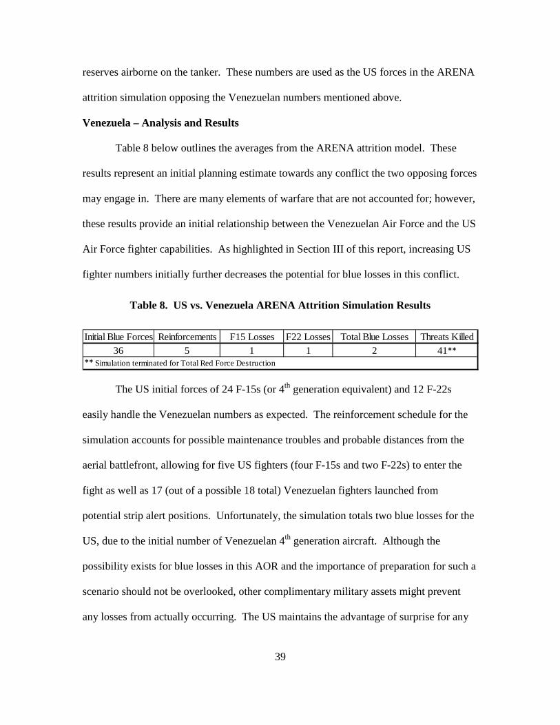
Table 8 below outlines the averages from the ARENA attrition model. These
results represent an initial planning estimate towards any conflict the two opposing forces
may engage in. There are many elements of warfare that are not accounted for; however,
these results provide an initial relationship between the Venezuelan Air Force and the US
Air Force fighter capabilities. As highlighted in Section III of this report, increasing US
fighter numbers initially further decreases the potential for blue losses in this conflict.
Table 8. US vs. Venezuela ARENA Attrition Simulation Results
Initial Blue Forces Reinforcements F15 Losses F22 Losses Total Blue Losses Threats Killed36 5 1 1 2 41**
** Simulation terminated for Total Red Force Destruction
The US initial forces of 24 F-15s (or 4th generation equivalent) and 12 F-22s
easily handle the Venezuelan numbers as expected. The reinforcement schedule for the
simulation accounts for possible maintenance troubles and probable distances from the
aerial battlefront, allowing for five US fighters (four F-15s and two F-22s) to enter the
fight as well as 17 (out of a possible 18 total) Venezuelan fighters launched from
potential strip alert positions. Unfortunately, the simulation totals two blue losses for the
US, due to the initial number of Venezuelan 4th generation aircraft. Although the
possibility exists for blue losses in this AOR and the importance of preparation for such a
scenario should not be overlooked, other complimentary military assets might prevent
any losses from actually occurring. The US maintains the advantage of surprise for any

40
conflict that takes place on foreign soil or above foreign territory. This conflict would
more than likely consist of cruise missiles or other standoff weapons, alongside of space
and cyberspace assets targeted at strategic nodes intended to weaken the Venezuelan
political and military structure; occurring simultaneously with the first US aircraft being
launched. This surprise greatly impacts Venezuela’s fighter force’s ability to find and
target US aircraft before being completely destroyed. The blue loss numbers that are
output from the ARENA attrition model should be treated as simply the result of force-
on-force conflict, absent of the other noteworthy advantages the US military maintains
over its adversaries and represents more closely a worst-case outcome.
IRAN – Moderate Technology, Moderate Numbers
The Islamic Republic of Iran Air Force represents a handful of countries
worldwide that have a moderately sized force utilizing some elements of technology that
enhance their lethality and/or survivability. Their government is aligned in opposition to
the United States and takes opportunity to voice their dissent on a regular basis. There is
a growing concern from the global populace that Iran is taking measures towards
securing nuclear capabilities, specifically efforts directed towards the creation of atomic
weapons. This represents a huge source of instability for the already volatile region and
increases the likelihood for future US involvement.
The Iranian Air Force is a hodge-podge of aircraft and capabilities resultant of
multiple conflicts and previous military acquisitions. Its composition, including
previously exported US fighters, is somewhat unique in regards to the potential threat
facing the US. As initially stated in the scenario control section, it is most difficult to
41
assess the operational status of these antiquated US exports due to the termination of all
parts and maintenance to Iran from the US many years ago. Another significant portion
of their fleet is remnant of the Gulf War in 1991, with multiple Iraqi aircraft acquired as
defectors during the conflict. None of these aircraft included any maintenance or
replacement parts and are questionable in their operation. Iran is in constant contact with
the Russian military industry and is suspected of attempting to acquire modern fighters;
however, as of this publication, none are known to have exchanged hands. The most
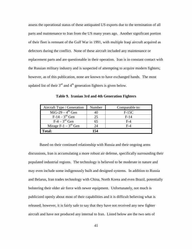
updated list of their 3rd and 4th generation fighters is given below.
Table 9. Iranian 3rd and 4th Generation Fighters
Aircraft Type / Generation Number Comparable to: MiG-29 – 4th Gen 40 F-15C
F-14 – 3rd Gen 25 F-14 F-4 – 3rd Gen 65 F-4
Mirage F-1 – 3rd Gen 24 F-4 Total: 154
Based on their continued relationship with Russia and their ongoing arms
discussions, Iran is accumulating a more robust air defense, specifically surrounding their
populated industrial regions. The technology is believed to be moderate in nature and
may even include some indigenously built and designed systems. In addition to Russia
and Belarus, Iran trades technology with China, North Korea and even Brazil, potentially
bolstering their older air force with newer equipment. Unfortunately, not much is
publicized openly about most of their capabilities and it is difficult believing what is
released; however, it is fairly safe to say that they have not received any new fighter
aircraft and have not produced any internal to Iran. Listed below are the two sets of

42
attrition coefficient scorecards. Of note, the Iranian Air Force receives slightly higher
values than Venezuela due to suspected EA on some of their 3rd generation fighters.

43
Table 10. Solving for US vs. Iran Attrition Coefficients
United States 5th Gen v. 4th Gen 5th Gen v. 3rd Gen 4th Gen v. 4th Gen 4th Gen v. 3rd Gen Fighter Gen Advantage = 0.4 Advantage = 0.8 Same = 0.0 Advantage = 0.4 TTPs/Training Advantage = 0.4 Advantage = 0.4 Advantage = 0.4 Advantage = 0.4 Technology Advantage = 0.4 Advantage = 0.4 Advantage = 0.4 Advantage = 0.4 Stealth Yes = 0.5 Yes = 0.5 No = 0.0 No = 0.0 EA None = 0.0 None = 0.0 20% Decrease = 0.2 20% Decrease = 0.2 Time Constant = 0.6 = 0.6 = 0.6 = 0.6 Fighter Gen Multiplier 5th Generation = 1.0 5th Generation = 1.0 4th Generation = 0.8 4th Generation = 0.8
Attrition Coefficient: α = 3.3 β = 3.7 χ = 2.4 δ =2.8
Table 11. Solving for Iran vs. US Attrition Coefficients
Iran 4th Gen v. 5th Gen 3rd Gen v. 5th Gen 4th Gen v. 4th Gen 3rd Gen v. 4th Gen Fighter Gen Disadvantage = -0.4 Disadvantage = -0.4 Same = 0.0 Disadvantage = -0.4 TTPs/Training Disadvantage = -0.4 Disadvantage = -0.4 Disadvantage = -0.4 Disadvantage = -0.4 Technology Disadvantage = -0.4 Disadvantage = -0.4 Disadvantage = -0.4 Disadvantage = -0.4 Stealth No = 0.0 No = 0.0 No = 0.0 No = 0.0 EA 20% Decrease = 0.2 20% Decrease = 0.2 20% Decrease = 0.2 20% Decrease = 0.2 Time Constant = 0.6 = 0.6 = 0.6 = 0.6 Fighter Gen Multiplier 4th Generation = 0.8 3rd Generation = 0.6 4th Generation = 0.8 3rd Generation = 0.6
Attrition Coefficient: ε = 0.4 φ = 0.2 γ = 0.8 η =0.2
Conflict Specifics
The geographic layout of Iran is much greater than that previously discussed with
Venezuela. Any conflict held in the Iranian airspace would initially be localized to
achieve air superiority only during the window of ground strikes by conventional (non-
stealth) bombers. Air superiority forces would withdraw until the next series of strikes
and then establish local air superiority again and would continue to do so, until the
Iranian air defenses were softened, strategic targets were destroyed and forward basing of
fighters could take place, allowing for continuous air superiority. This approach to
gaining air dominance is the most likely option for AORs of massive scale. Although the
44
Iranian territory is spread out, it is safe to conclude that most of their fighters are
centralized around their strategic centers of gravity, specifically around Tehran and
Esfahan. A potential aerial battle might take place on the outer perimeters of this central
region, consisting of a large number of the Iranian forces that are operational. Seventy
percent of the fighters listed in Table 9 are assumed to be available, divided into initial
forces and reinforcements from the surrounding bases. This force strength of 108 fighters
is easily contested; however, the salient points of discussion involve an increase in
numbers and some increase in technology over the previous example.
Contrary to the Venezuelan case study, the United States total numbers involved
would be much greater; however, those initially dedicated to any specific mission such as
gaining air superiority over a localized area, would be of similar nature, 24 F-15s and 12
F-22s. These numbers are used for the initial US force strength; however, a significant
increase in reinforcement numbers is simulated representing greater forces available for
the larger conflict. These forces would come from a nearby aircraft carrier, if close to
one of the seas, or direct from a nearby air-refueling track.
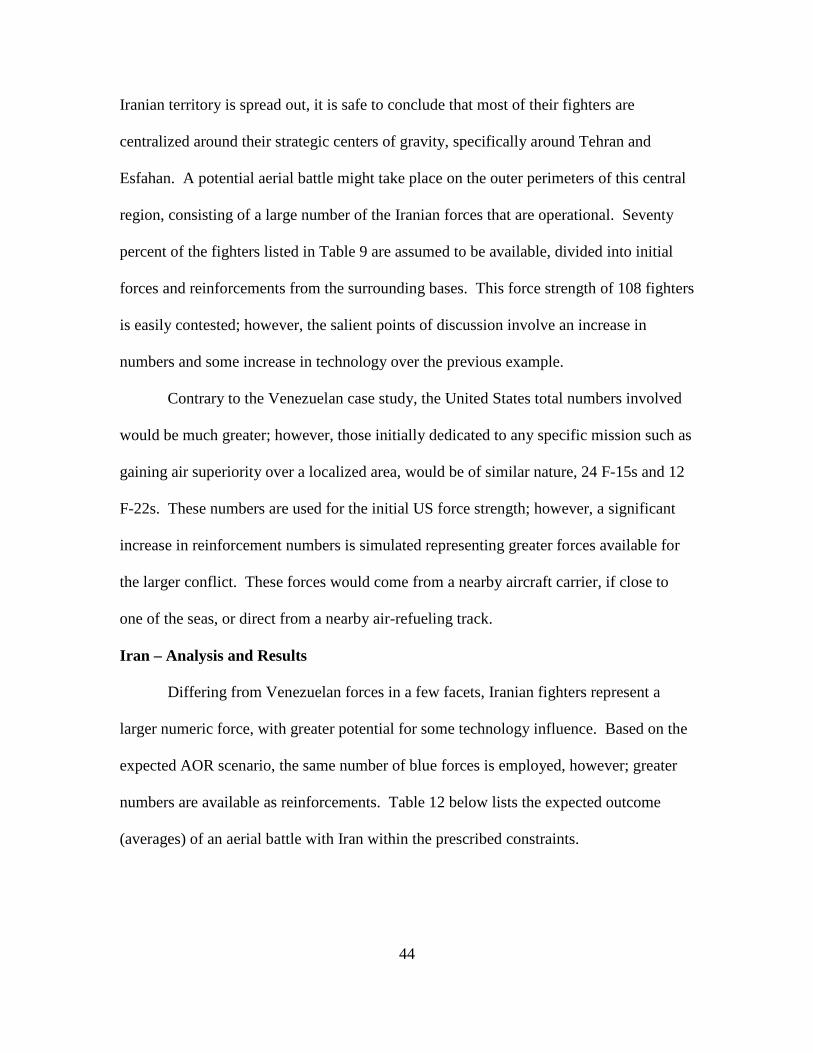
Iran – Analysis and Results
Differing from Venezuelan forces in a few facets, Iranian fighters represent a
larger numeric force, with greater potential for some technology influence. Based on the
expected AOR scenario, the same number of blue forces is employed, however; greater
numbers are available as reinforcements. Table 12 below lists the expected outcome
(averages) of an aerial battle with Iran within the prescribed constraints.
45
It is apparent from the Section III analysis that greater threat numbers result in a
larger number of blue total force losses. Larger threat numbers are coupled with the
expectation for slightly more EA, specifically equipped on the 3rd generation aircraft,
unlike Venezuela. These inputs increase the blue losses over the previous case study to
five. The total number of threats killed is 64 resulting in the localized fighting to be
terminated and air superiority to be established by the US fighters. Due to the time
elapsed, six US reinforcement fighters (four F-15s and two F-22s) entered the fight, while
14 threat fighters scrambled from their ground alert to join the battle and subsequently be
shot down. As discussed with the Venezuelan analysis, an increase in the initial numbers
of US fighters directly decreases the expected blue losses. Additionally, it is important to
once again consider that any conflict over Iran is initiated on the terms of the US,
employing its full arsenal of military capabilities that significantly impacts the Iranian
force’s ability to launch and direct their fighters appropriately.
China – High Technology, High Numbers
The Peoples Republic of China represents the worst possible scenario for the
United States military in many circumstances. The rapid evolution of their military is
unmatched for nearly a decade now, laying the foundation for advanced capabilities in
the air, on the land, and patrolling the seas. In addition to their conventional military
forces, their expansion into the domains of space and cyberspace bolsters their global
Table 12. US vs. Iran ARENA Attrition Simulation Results

46
presence and cements their dominance in the Pacific. Their current strength is arguably
on par with the United States’ military’s ability to wage war in the region; however, the
rate of expansion into developing technologies is without equal and may soon (if not
already) fortify their position at the top in the global arena. China’s level of technology
is considered amongst the highest, placing them in the top tier of world countries and
their aircraft numbers, comprised of the People’s Liberation Army Air Force (PLAAF)
and People’s Liberation Army Navy (PLAN) assets exceed all but the United States
currently.
Table 13. Chinese 3rd and 4th Generation Fighters
Aircraft Type / Generation Number Comparable to: Su-30MKK/MK2 – 4th Gen 127 F-15E Su-27SK/J-11B – 4th Gen 132 F-15C/F-15E
J-10 – 4th Gen 80 F-16 J-8 – 3rd Gen 390 F-4 / MiG-23 J-7 – 3rd Gen 579 F-5 / MiG-21
JH-7 – 3rd Gen 70 F-111 Total: 1378
Listed above is a summary of China’s fighter aircraft, not including any bomber,
reconnaissance, light attack, command and control, or other aircraft of various utilities.
Only 3rd and 4th generation aircraft are listed; however, it is important to note, that
China is currently in development of their first 5th generation fighter, the J-20, which is
claimed to be similar in capability to the F-22A, employing stealth technology, advanced
integrated avionics and a sensor suite that allows for increased battlefield awareness.
Additionally, it is rumored that China already has or is currently in the process of
converting hundreds of their 1st and 2nd generation fighters into unmanned drones, intent
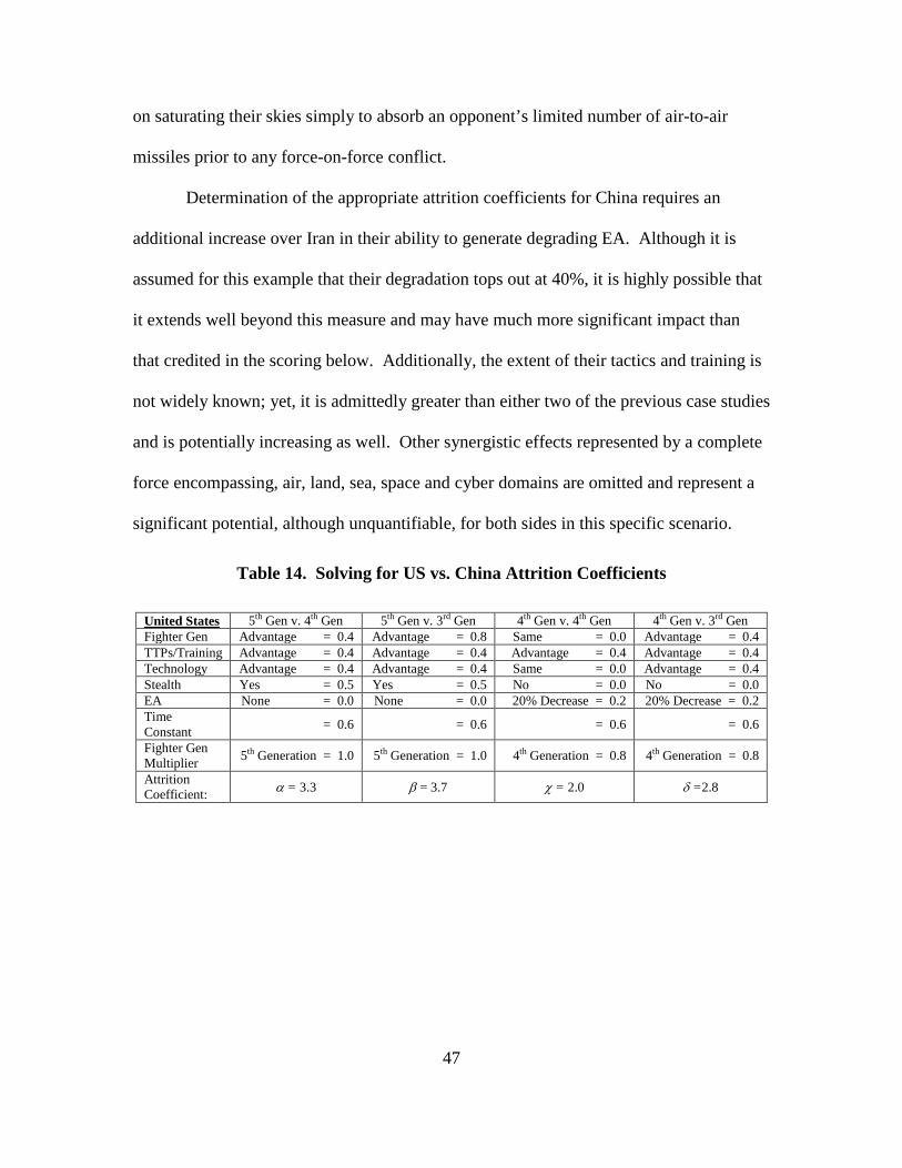
47
on saturating their skies simply to absorb an opponent’s limited number of air-to-air
missiles prior to any force-on-force conflict.
Determination of the appropriate attrition coefficients for China requires an
additional increase over Iran in their ability to generate degrading EA. Although it is
assumed for this example that their degradation tops out at 40%, it is highly possible that
it extends well beyond this measure and may have much more significant impact than
that credited in the scoring below. Additionally, the extent of their tactics and training is
not widely known; yet, it is admittedly greater than either two of the previous case studies
and is potentially increasing as well. Other synergistic effects represented by a complete
force encompassing, air, land, sea, space and cyber domains are omitted and represent a
significant potential, although unquantifiable, for both sides in this specific scenario.
Table 14. Solving for US vs. China Attrition Coefficients
United States 5th Gen v. 4th Gen 5th Gen v. 3rd Gen 4th Gen v. 4th Gen 4th Gen v. 3rd Gen Fighter Gen Advantage = 0.4 Advantage = 0.8 Same = 0.0 Advantage = 0.4 TTPs/Training Advantage = 0.4 Advantage = 0.4 Advantage = 0.4 Advantage = 0.4 Technology Advantage = 0.4 Advantage = 0.4 Same = 0.0 Advantage = 0.4 Stealth Yes = 0.5 Yes = 0.5 No = 0.0 No = 0.0 EA None = 0.0 None = 0.0 20% Decrease = 0.2 20% Decrease = 0.2 Time Constant = 0.6 = 0.6 = 0.6 = 0.6
Fighter Gen Multiplier 5th Generation = 1.0 5th Generation = 1.0 4th Generation = 0.8 4th Generation = 0.8
Attrition Coefficient: α = 3.3 β = 3.7 χ = 2.0 δ =2.8
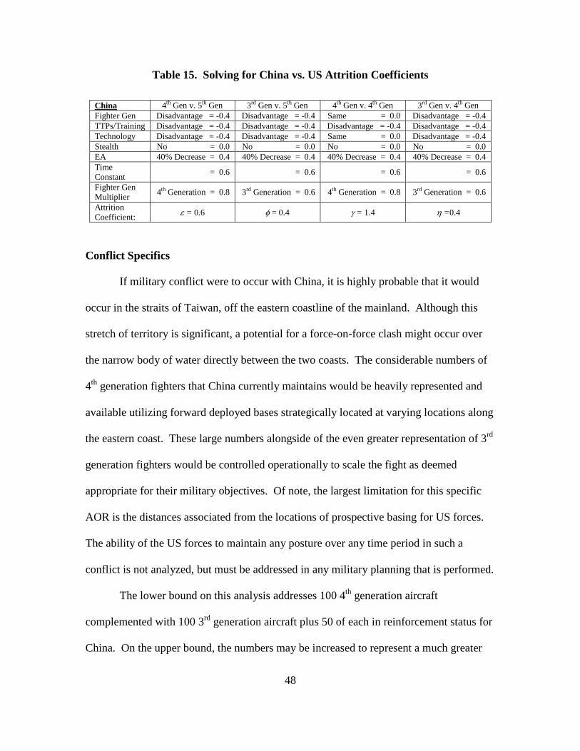
48
Table 15. Solving for China vs. US Attrition Coefficients
China 4th Gen v. 5th Gen 3rd Gen v. 5th Gen 4th Gen v. 4th Gen 3rd Gen v. 4th Gen Fighter Gen Disadvantage = -0.4 Disadvantage = -0.4 Same = 0.0 Disadvantage = -0.4 TTPs/Training Disadvantage = -0.4 Disadvantage = -0.4 Disadvantage = -0.4 Disadvantage = -0.4 Technology Disadvantage = -0.4 Disadvantage = -0.4 Same = 0.0 Disadvantage = -0.4 Stealth No = 0.0 No = 0.0 No = 0.0 No = 0.0 EA 40% Decrease = 0.4 40% Decrease = 0.4 40% Decrease = 0.4 40% Decrease = 0.4 Time Constant = 0.6 = 0.6 = 0.6 = 0.6
Fighter Gen Multiplier 4th Generation = 0.8 3rd Generation = 0.6 4th Generation = 0.8 3rd Generation = 0.6
Attrition Coefficient: ε = 0.6 φ = 0.4 γ = 1.4 η =0.4
Conflict Specifics
If military conflict were to occur with China, it is highly probable that it would
occur in the straits of Taiwan, off the eastern coastline of the mainland. Although this
stretch of territory is significant, a potential for a force-on-force clash might occur over
the narrow body of water directly between the two coasts. The considerable numbers of
4th generation fighters that China currently maintains would be heavily represented and
available utilizing forward deployed bases strategically located at varying locations along
the eastern coast. These large numbers alongside of the even greater representation of 3rd
generation fighters would be controlled operationally to scale the fight as deemed
appropriate for their military objectives. Of note, the largest limitation for this specific
AOR is the distances associated from the locations of prospective basing for US forces.
The ability of the US forces to maintain any posture over any time period in such a
conflict is not analyzed, but must be addressed in any military planning that is performed.
The lower bound on this analysis addresses 100 4th generation aircraft
complemented with 100 3rd generation aircraft plus 50 of each in reinforcement status for
China. On the upper bound, the numbers may be increased to represent a much greater

49
portion of the Chinese force, although as determined below, this is largely unnecessary
due to consistent conclusions reached at the smaller force level. The US numbers
represent eight F-15C squadrons (4th generation) and four F-22 squadrons (fifth
generation) deployed to locations as available near the AOR. This number of squadrons
is able to support 48 F-15s and 24 F-22s for the initial fight and half of that (24 F-15s and
12 F-22s) in reserve on a nearby tanker.
China – Analysis and Results
A significant disparity is noticed immediately with the output of the ARENA
attrition model for China in comparison to the other two case studies. Based on the
sizeable initial force of 3rd and 4th generation fighters and the increased technological
capability that presents itself in greater EA degradation, China is able to defeat the entire
blue force of 64 F-15Cs and 32 F-22s (initial force and reinforcements). This result leads
to running the simulation again with increased initial blue forces and results in similar
output. The second set of data highlights total destruction of the US fighters once more;
however, the increased blue numbers delay the outcome allowing more reinforcements to
arrive, while destroying almost twice as many Chinese aircraft. This iteration of blue
initial strength is repeated to determine the point of inflection, representing the smaller
blue force attrition rate as demonstrated in Section III. Captured below in Table 16 are
the average results of each of the five separate tests, run ten times each to account for the
stochastic effect of maintenance variation, each representing a different blue force initial
strength.
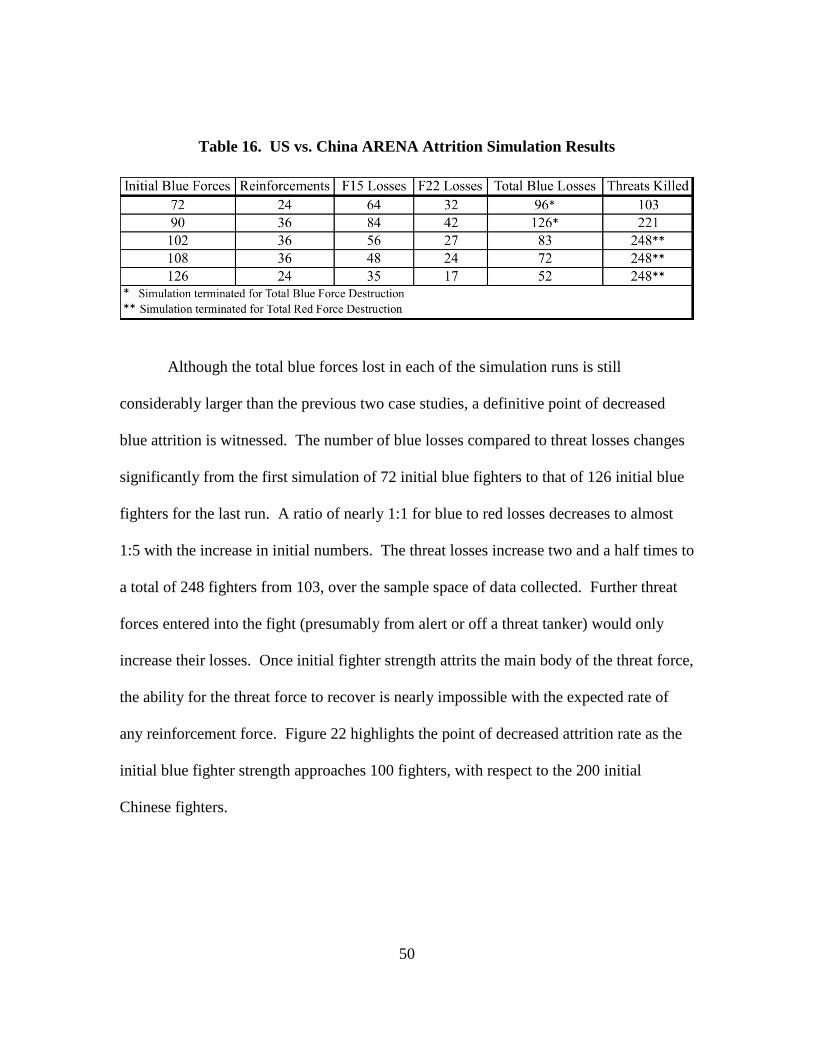
50
Although the total blue forces lost in each of the simulation runs is still
considerably larger than the previous two case studies, a definitive point of decreased
blue attrition is witnessed. The number of blue losses compared to threat losses changes
significantly from the first simulation of 72 initial blue fighters to that of 126 initial blue
fighters for the last run. A ratio of nearly 1:1 for blue to red losses decreases to almost
1:5 with the increase in initial numbers. The threat losses increase two and a half times to
a total of 248 fighters from 103, over the sample space of data collected. Further threat
forces entered into the fight (presumably from alert or off a threat tanker) would only
increase their losses. Once initial fighter strength attrits the main body of the threat force,
the ability for the threat force to recover is nearly impossible with the expected rate of
any reinforcement force. Figure 22 highlights the point of decreased attrition rate as the
initial blue fighter strength approaches 100 fighters, with respect to the 200 initial
Chinese fighters.
Table 16. US vs. China ARENA Attrition Simulation Results
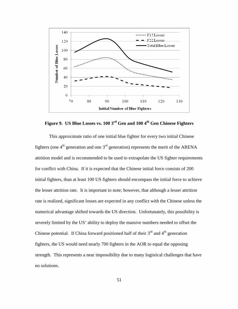
51
Figure 9. US Blue Losses vs. 100 3rd Gen and 100 4th Gen Chinese Fighters
This approximate ratio of one initial blue fighter for every two initial Chinese
fighters (one 4th generation and one 3rd generation) represents the merit of the ARENA
attrition model and is recommended to be used to extrapolate the US fighter requirements
for conflict with China. If it is expected that the Chinese initial force consists of 200
initial fighters, than at least 100 US fighters should encompass the initial force to achieve
the lesser attrition rate. It is important to note; however, that although a lesser attrition
rate is realized, significant losses are expected in any conflict with the Chinese unless the
numerical advantage shifted towards the US direction. Unfortunately, this possibility is
severely limited by the US’ ability to deploy the massive numbers needed to offset the
Chinese potential. If China forward positioned half of their 3rd and 4th generation
fighters, the US would need nearly 700 fighters in the AOR to equal the opposing
strength. This represents a near impossibility due to many logistical challenges that have
no solutions.
52
V. Conclusions and Recommendations
Mathematical analysis provides a foundation for the political and military
decisions surrounding fighter force manning, specifically the number of aircraft required
to combat given threat scenarios. As demonstrated in the case studies of Venezuela and
Iran, the current force structure is adequate and continues to be sufficient for any conflict
representative in nature of low to moderate fighters numbers with low to moderate
technology and capabilities. Although the US’ force composition will continue to
decrease over the next five years as the F-15, F-16 and F-18 fleets diminish, taking the
fighter inventory to historical lows, the US’ ability to project presence into AORs of low
to moderate posture remains uninterrupted. Once the eventual F-35 production is at full
strength and substantial numbers are rolling off the production line annually, the US’
fighter strength will be renewed to match that of the past thirty years.
Unfortunately, none of this optimistic projection answers the present numeric
challenges that are at hand with China or any other country that demonstrates
technological advances alongside of growing inventory. Although the list of countries
equipped with high numbers and high technology is fairly limited, arguably Russia, India
and the aforementioned China, the evolution of tactical and operational capabilities may
marginalize the United States’ fighter force’s strength altogether. Certain environments
are growing less advantageous and the US’ global might is slipping as it fails to account
for the expanding threat basis. Mathematically, there are various assumptions that
accompany any analysis; however, even if the assumptions represented in the attrition
coefficient determination are tilted towards the US favor and if the initial fighter
53
numbers, reinforcement numbers or reinforcement arrival schedule are adjusted to the
benefit of the US, the outcome is still highly undesirable and the consequences are
undeniably grave. This quantifiable understanding provides structure to the previous
rhetoric of declining fighter numbers and the resultant declining strategic global
influence. There is no refuting the military implications of a lesser force in this
circumstance.
All is not lost in respect to the growing hegemony represented by China, India or
that previously understood by Russia. Although the US acquisition timeline is
disadvantageous with respect to impacting the sliding numerical difference between
fighter aircraft, technology may be utilized to maintain its battlefield advantage.
Advancement in missile technology to ensure survivability in a dense EA environment
increases the effectiveness and produces more air-to-air victories per missile fired.
Limitations to the currently fielded BVR missiles are discussed at length in open-forum.
Advances in guidance logic makes it possible to target an identified threat with off-board
sensors that are dispersed, vast and inter-connected such that no missile guidance is
reliant upon a single sensor that may be easily jammed, causing failure. This off-board
cueing takes advantages of multi-spectral sensors comprising a network of platforms that
collectively build, maintain and map out an entire battlefield, in the air and on the ground.
Most of this technology is inexpensive comparatively and represents a redundant system
of varied capabilities overlapped to ensure constant coverage of the desired area,
providing consummate battlefield situational awareness.
Additional areas for technology expansion include but are not limited to:
increased missile kinematics, smaller missiles of similar capability, increased electronic

54
attack whether internally configured or externally mounted, multi-spectral sensor
utilization such as an IRST on most fighters, and unmanned platforms of varying
capacity. Spending drastically less money and acquiring advanced capabilities in a
considerably shortened period is an answer to the current economic constraints and the
impending decrease in the US’ numerical representation. These technology
developments directly impact the lethality or survivability of US forces, providing a new
tactical margin on the battlefield and hopefully accounting for any disparity encountered.
Further mathematical study is recommended, employing various techniques to
better quantify the growing problem and addressing potential solutions to the United
States’ air superiority concerns. Application of Lanchester differential equations to
anticipate potential blue force attrition for actual CONPLANs and OPLANs, would refine
the next level of analysis and better describe the actual requirements. Attrition
coefficient determination using scoring methods as discussed in this research could be
built upon drawing greater detail from existing capabilities, potentially applying a
weighting scale to those characteristics more crucial to survival or those that significantly
increase lethality. This weighting of characteristics might better represent the actual
threat environment operating in, accounting directly for adversarial capabilities in true
sense instead of simplistic 3rd and 4th generation generalities. The Lanchester differential
equations could be supplemented to capture threat surface-to-air missile numbers,
location and capabilities, adding complexity to this basic research that would better
quantify the results from one AOR to another. Lastly, all assumptions for force
composition, capabilities, reinforcement schedules and basing expectations could be
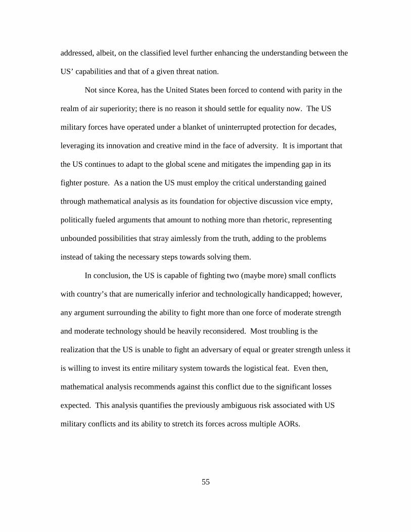
55
addressed, albeit, on the classified level further enhancing the understanding between the
US’ capabilities and that of a given threat nation.
Not since Korea, has the United States been forced to contend with parity in the
realm of air superiority; there is no reason it should settle for equality now. The US
military forces have operated under a blanket of uninterrupted protection for decades,
leveraging its innovation and creative mind in the face of adversity. It is important that
the US continues to adapt to the global scene and mitigates the impending gap in its
fighter posture. As a nation the US must employ the critical understanding gained
through mathematical analysis as its foundation for objective discussion vice empty,
politically fueled arguments that amount to nothing more than rhetoric, representing
unbounded possibilities that stray aimlessly from the truth, adding to the problems
instead of taking the necessary steps towards solving them.
In conclusion, the US is capable of fighting two (maybe more) small conflicts
with country’s that are numerically inferior and technologically handicapped; however,
any argument surrounding the ability to fight more than one force of moderate strength
and moderate technology should be heavily reconsidered. Most troubling is the
realization that the US is unable to fight an adversary of equal or greater strength unless it
is willing to invest its entire military system towards the logistical feat. Even then,
mathematical analysis recommends against this conflict due to the significant losses
expected. This analysis quantifies the previously ambiguous risk associated with US
military conflicts and its ability to stretch its forces across multiple AORs.

56
Appendix A. List of Abbreviations and Acronyms
ACC – Air Combat Command
AOR – Area of Responsibility
BVR – Beyond Visual Range
CAF – Combat Air Forces
CONPLAN – Conceptual Plan
DACT – Dissimilar Air Combat Training
EA – Electronic Attack
EP – Emergency Procedure
F – Fighter
FLCS – Flight Control System
HOTAS – Hands on Throttles and Stick
HUD – Heads Up Display
IR – Infrared
IRST – Infrared Search and Track
LGB – Laser Guided Bomb
LtGen – Lieutenant General
Me – Messerschmitt
MiG – Mikoyan Gurevich
OPLAN – Operation Plan
Pk – Probability of Kill
RADAR – Radio Detection and Ranging
SAM – Surface-to-Air Missile
SAR – Synthetic Aperture RADAR
SCL – Standard Conventional Load
Su – Sukhoi
TRIA – Triangular Distribution
UNIF – Uniform Distribution
US – United States
USAF – United States Air Force
WVR – Within Visual Range
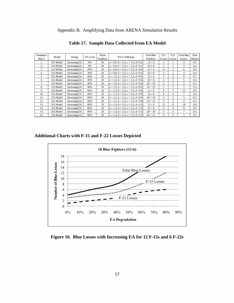
57
Appendix B. Amplifying Data from ARENA Simulation Results
Table 17. Sample Data Collected from EA Model
Simulation Run # Model Testing EA Level
Threat Numbers Test Coefficients
Total Blue Numbers
F15 Losses
F22 Losses
Total Blue Losses
Time (hours)
1 EA Model Increasing EA 0% 20 a = 0.6, b = 2.4, c = 3.3, d =0.2 12 + 6 3 1 4 0.52 EA Model Increasing EA 0% 20 a = 0.6, b = 2.4, c = 3.3, d =0.2 16 + 8 2 1 3 0.43 EA Model Increasing EA 20% 20 a = 0.8, b = 2.4, c = 3.3, d =0.4 12 + 6 4 2 6 0.64 EA Model Increasing EA 20% 20 a = 0.8, b = 2.4, c = 3.3, d =0.4 16 + 8 3 1 4 0.45 EA Model Increasing EA 40% 20 a = 1.0, b = 2.4, c = 3.3, d =0.6 12 + 6 5 3 8 0.76 EA Model Increasing EA 40% 20 a = 1.0, b = 2.4, c = 3.3, d =0.6 16 + 8 3 2 5 0.47 EA Model Increasing EA 40% 20 a = 1.0, b = 2.4, c = 3.3, d =0.6 20 + 10 3 2 5 0.38 EA Model Increasing EA 40% 20 a = 1.0, b = 2.4, c = 3.3, d =0.6 24 + 12 2 1 3 0.39 EA Model Increasing EA 60% 20 a = 1.2, b = 2.4, c = 3.3, d =0.8 12 + 6 8 5 13 0.910 EA Model Increasing EA 60% 20 a = 1.2, b = 2.4, c = 3.3, d =0.8 16 + 8 4 3 7 0.411 EA Model Increasing EA 60% 20 a = 1.2, b = 2.4, c = 3.3, d =0.8 20 + 10 3 2 5 0.312 EA Model Increasing EA 60% 20 a = 1.2, b = 2.4, c = 3.3, d =0.8 24 + 12 2 2 4 0.313 EA Model Increasing EA 80% 20 a = 1.4, b = 2.4, c = 3.3, d =1.0 12 + 6 12 6 18 0.914 EA Model Increasing EA 80% 20 a = 1.4, b = 2.4, c = 3.3, d =1.0 16 + 8 5 4 9 0.515 EA Model Increasing EA 80% 20 a = 1.4, b = 2.4, c = 3.3, d =1.0 20 + 10 4 3 7 0.316 EA Model Increasing EA 80% 20 a = 1.4, b = 2.4, c = 3.3, d =1.0 24 + 12 3 2 5 0.3
Additional Charts with F-15 and F-22 Losses Depicted
Figure 10. Blue Losses with Increasing EA for 12 F-15s and 6 F-22s

58
Figure 11. Blue Losses with Increasing EA for 16 F-15s and 8 F-22s
Figure 12. Blue Losses with Increasing EA for 20 F-15s and 10 F-22s

59
Figure 13. Blue Losses with Increasing EA for 24 F-15s and 12 F-22s
Figure 14. Blue Losses with No EA and Increasing Initial Force Strength
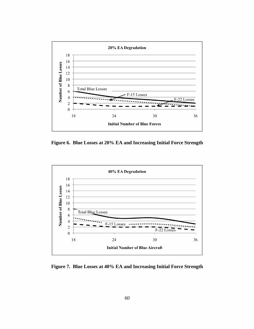
60
Figure 6. Blue Losses at 20% EA and Increasing Initial Force Strength
Figure 7. Blue Losses at 40% EA and Increasing Initial Force Strength
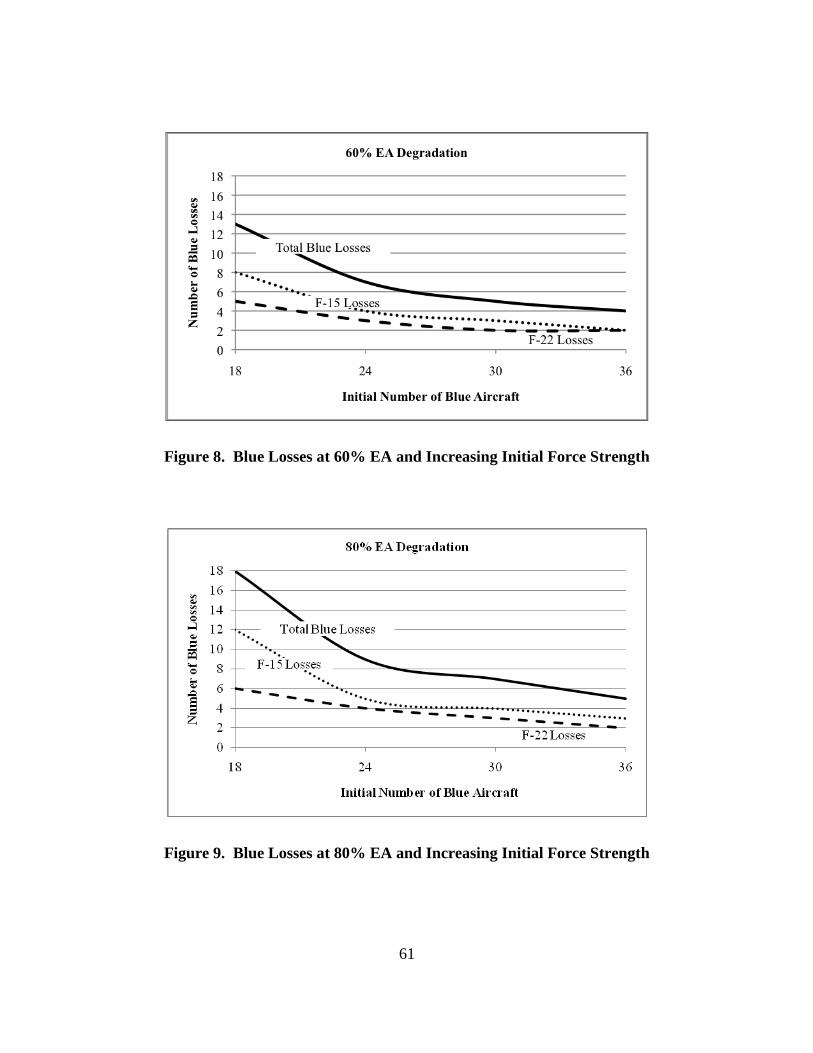
61
Figure 8. Blue Losses at 60% EA and Increasing Initial Force Strength
Figure 9. Blue Losses at 80% EA and Increasing Initial Force Strength
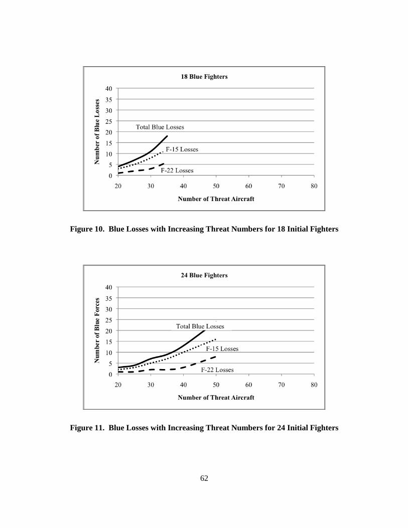
62
Figure 10. Blue Losses with Increasing Threat Numbers for 18 Initial Fighters
Figure 11. Blue Losses with Increasing Threat Numbers for 24 Initial Fighters
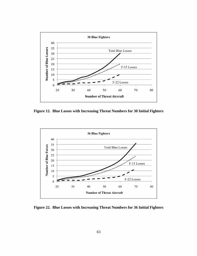
63
Figure 12. Blue Losses with Increasing Threat Numbers for 30 Initial Fighters
Figure 22. Blue Losses with Increasing Threat Numbers for 36 Initial Fighters

64
Table 18. Sample Data of Replications from Venezuela Case Study
ReplicationF15
ReinforcementsF22
ReinforcementsF15
LossesF22
LossesTotal Blue
Losses4th Gen Threat
Losses3rd Gen Threat
Losses1 3.5 2 1.5 1 2.5 31.25 112 3.5 1.5 1.5 0.5 2 30.5 113 3.25 2 1.25 1 2.25 30.5 10.54 3.25 2 1.25 1 2.25 30.75 10.55 3.25 0.5 1.25 0.5 1.75 30.25 116 3.5 1.5 1.5 0.5 2 30.25 10.257 2.25 1 1.25 1 2.25 30.5 118 3.25 2 1.25 1 2.25 30.25 10.59 3.5 2 1.5 1 2.5 30.25 1110 3.25 2 1.25 1 2.25 30.5 11
Average 3.25 1.65 1.35 0.85 2.2 30.5 10.775Standard Dev 0.354 0.502 0.122 0.229 0.218 0.296 0.284
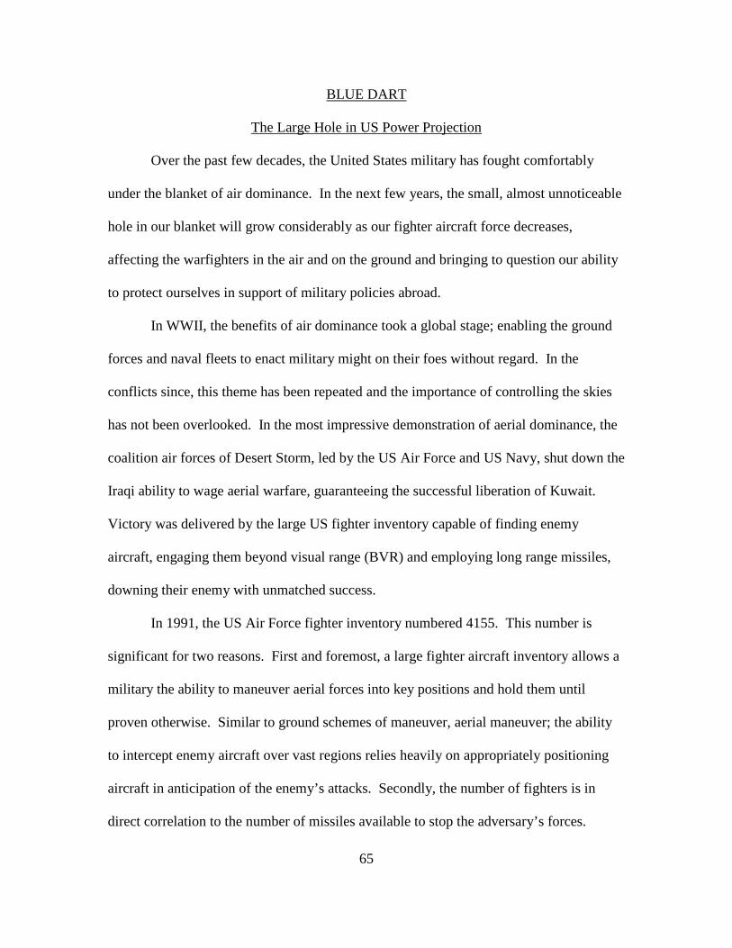
65
BLUE DART
The Large Hole in US Power Projection
Over the past few decades, the United States military has fought comfortably
under the blanket of air dominance. In the next few years, the small, almost unnoticeable
hole in our blanket will grow considerably as our fighter aircraft force decreases,
affecting the warfighters in the air and on the ground and bringing to question our ability
to protect ourselves in support of military policies abroad.
In WWII, the benefits of air dominance took a global stage; enabling the ground
forces and naval fleets to enact military might on their foes without regard. In the
conflicts since, this theme has been repeated and the importance of controlling the skies
has not been overlooked. In the most impressive demonstration of aerial dominance, the
coalition air forces of Desert Storm, led by the US Air Force and US Navy, shut down the
Iraqi ability to wage aerial warfare, guaranteeing the successful liberation of Kuwait.
Victory was delivered by the large US fighter inventory capable of finding enemy
aircraft, engaging them beyond visual range (BVR) and employing long range missiles,
downing their enemy with unmatched success.
In 1991, the US Air Force fighter inventory numbered 4155. This number is
significant for two reasons. First and foremost, a large fighter aircraft inventory allows a
military the ability to maneuver aerial forces into key positions and hold them until
proven otherwise. Similar to ground schemes of maneuver, aerial maneuver; the ability
to intercept enemy aircraft over vast regions relies heavily on appropriately positioning
aircraft in anticipation of the enemy’s attacks. Secondly, the number of fighters is in
direct correlation to the number of missiles available to stop the adversary’s forces.

66
Without platforms capable of carrying the BVR weaponry, the ability to secure the skies
may be in question. It is troubling to think of defensive forces overrun, or escorting
fighters running out of munitions while protecting our strategic bombing campaign.
Today, our current fighter aircraft number 2265 and are diminishing due to
increasing age and budget constraints. The lack of fighter numbers is further amplified
by the massive reduction in F-22s purchased and increasing delays of the F-35. The
newer, stealth fighters are multi-roled, responsible for not only air superiority but
precision attack as well, shifting ordnance load outs to bombs in place of air dominance
air-to-air missiles. This is significant due to the fact that all weapons are carried
internally maintaining the advanced fighters’ stealth signatures and every bomb carried
equals less missiles carried. The table below indicates the total number of fighter aircraft
available and BVR missile quantities represented by today’s inventory.
* Number of BVR missiles available if carrying bombs
These numbers may initially appear large, however; not all aircraft deploy during conflict
and not all fighter aircraft launch during a single mission. This table indicates that
although the new fighters are technologically advanced they are not a direct replacement
for the historic numbers.
Concerns do not stop with the shortage of aircraft or missile numbers. The
evolution of missile defeating technology and tactics is increasing due to its hugely cost
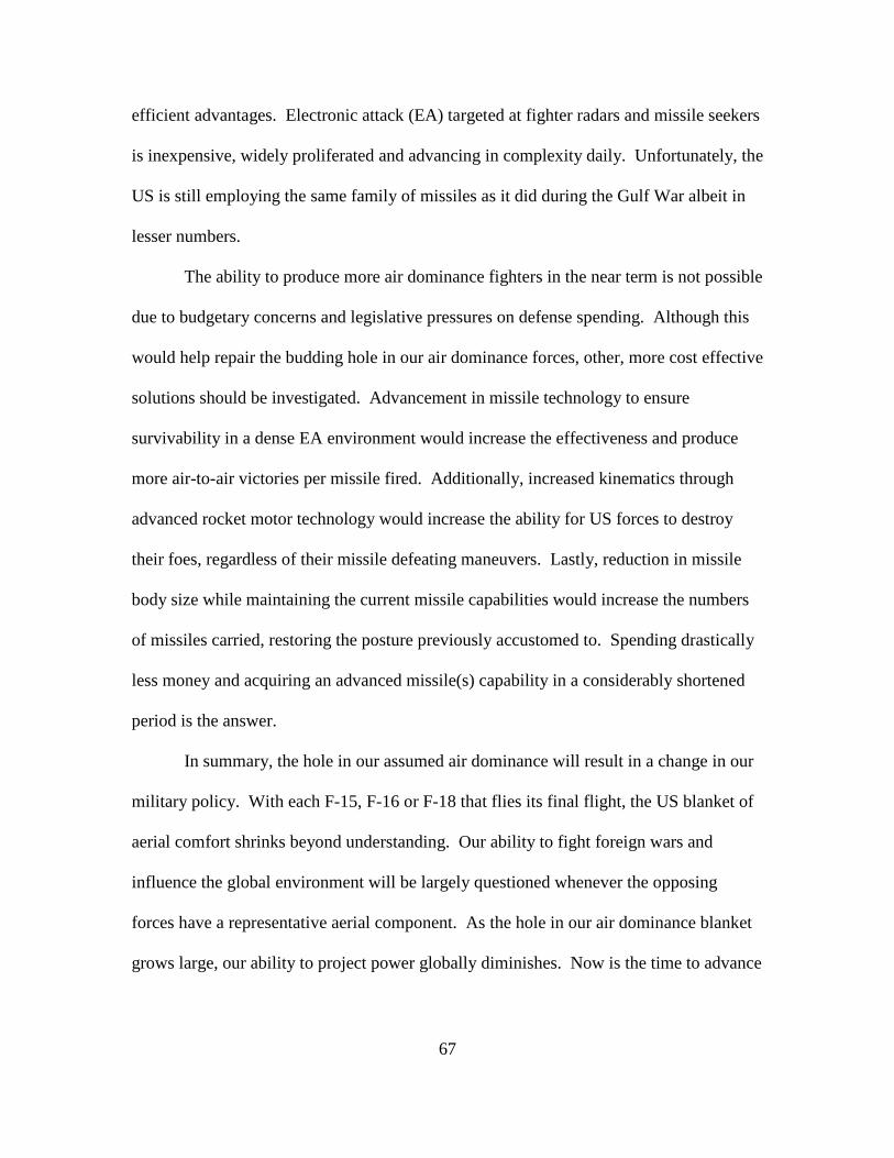
67
efficient advantages. Electronic attack (EA) targeted at fighter radars and missile seekers
is inexpensive, widely proliferated and advancing in complexity daily. Unfortunately, the
US is still employing the same family of missiles as it did during the Gulf War albeit in
lesser numbers.
The ability to produce more air dominance fighters in the near term is not possible
due to budgetary concerns and legislative pressures on defense spending. Although this
would help repair the budding hole in our air dominance forces, other, more cost effective
solutions should be investigated. Advancement in missile technology to ensure
survivability in a dense EA environment would increase the effectiveness and produce
more air-to-air victories per missile fired. Additionally, increased kinematics through
advanced rocket motor technology would increase the ability for US forces to destroy
their foes, regardless of their missile defeating maneuvers. Lastly, reduction in missile
body size while maintaining the current missile capabilities would increase the numbers
of missiles carried, restoring the posture previously accustomed to. Spending drastically
less money and acquiring an advanced missile(s) capability in a considerably shortened
period is the answer.
In summary, the hole in our assumed air dominance will result in a change in our
military policy. With each F-15, F-16 or F-18 that flies its final flight, the US blanket of
aerial comfort shrinks beyond understanding. Our ability to fight foreign wars and
influence the global environment will be largely questioned whenever the opposing
forces have a representative aerial component. As the hole in our air dominance blanket
grows large, our ability to project power globally diminishes. Now is the time to advance

68
our thinking, change our approach and ensure air dominance is ours for the future
generations ahead.

69
Bibliography
Anderson, Eric C. and Jeffrey G. Engstrom. Capabilities of the Chinese People
Liberation Army to Carry Out Military Action in the Event of a Regional Conflict. SAIC Corporation. March 2009.
Artelli, Michael J. and Richard F. Deckro. Modeling the Lanchester Laws with System
Dynamics. Aviation Week and Space Technology’s Aerospace 2010. Retrieved from
http://www.aviationweek.com/aw/generic/channel_awst.jsp?channel=awst on multiple occasions.
Baron, Kevin. “Retiring Air Force Intel Chief Sounds Alarm on American Air
Superiority.” Stars and Stripes. 14 September 2010. Bonder, S. “The Lanchester Attrition Rate Coefficient.” Operations Research. 1967 Caldwell and others. Aggregated Combat Models. Naval Postgraduate School. February
2000. Clark, Gordon M. “The Combat Analysis Model.” Proceedings of the 24th Military
Operations Research Symposium. November 1969. Cliff, Roger. The Development of China’s Air Force Capabilities: Testimony Presented
before US-China Economic and Security Review Commission. RAND Corporation. 20 May 2010.
Corley, John D. “Combat Air Power: The Need for a New Path.” Second Line of
Defense. August 2010a. -----. “The Future of Power Projection.” Second Line of Defense. September
2010b. Davis, Paul K. Aggregation, Disaggregation, and the 3:1 Rule in Ground Combat.
RAND Corporation. 1995.
Deptula, David. “Challenges to Air Superiority.” Second Line of Defense. October 2010.
-----. “The Chinese Challenge.” Second Line of Defense. January 2011a. -----. “The Evolution of PRC Air Power.” Second Line of Defense. January
2011b.

70
Drew, Donald R. and others. Systems Dynamics Modeling of Air Warfare. Virginia
Polytechnic Institute and State University. Grant, Rebecca. Combat Air Forces in Crisis. Mitchell Institute Study. Air Force
Association. March 2009a. -----. Losing Air Dominance. Mitchell Institute Study. Air Force
Association. September 2008. -----. The RADAR Game: Understanding Stealth and Aircraft
Survivability. Mitchell Institute Study. Air Force Association. September 2010. -----. The Vanishing Arsenal of Airpower. Mitchell Institute Study. Air Force
Association. October 2009b. Hartman, James K. High Resolution Combat Modeling. Unpublished Notes. 1985. Kelton, D. and others. Simulation with ARENA (5th Edition). New York: McGraw-Hill
Book Company, 2010. Laird, Robbin F. “A 21st Century Concept of Air and Military Operations.” Defense
Horizons. 66: 1-6. March 2009. -----. “Embrace the Air Power Revolution: US Can’t Approach 5th Gen Aircraft the Old
Way.” Second Line of Defense. February 2011. -----. “Re-Norming Air Operations.” Second Line of Defense. February 2011. Lanchester, Frederick W. Aircraft in Warfare: The Dawn of the Fourth Arm. London:
Constable and Company Limited, 1916. Martinez, Vince. “Defense Cuts in the Future: Service Level Adjustments Key to
Maintaining Operational Advantage.” Second Line of Defense. February 2011. -----. “Waging the Future Fight.” Second Line of Defense. November 2010. Ruehrmund, James C. and Christopher J. Bowie. Arsenal of Airpower: USAF Aircraft
Inventory 1950-2009. Mitchell Institute Study. Air Force Association. November 2010.
Sheppard, Chris. “The F-35 and Legacy Aircraft: The Case of the F-16 (Part 1).”
Second Line of Defense. March 2010a.
71
-----. “The F-35 and Legacy Aircraft: Towards a New Paradigm (Part 2).” Second Line of Defense. March 2010b.
Taylor, James G. Explicit Analytical Expression for a Lanchester Attrition-Rate
Coefficient for Bonder and Farrell’s m-Period Target-Engagement Policy. MOVES Academic Group. Naval Postgraduate School. 9 July 2001.
-----. Lanchester Models of Warfare, Volume I. Military Applications Section.
Operations Research Society of America. 1983a. -----. Lanchester Models of Warfare, Volume II. Military Applications Section.
Operations Research Society of America. 1983b. Wynn, Michael. “Re-Norming the Asymmetric Advantage in Air Dominance: Going to
War with the Air Force you Have.” Second Line of Defense. October 2010.
72
Vita
Major Ronald Gilbert graduated from Norte Vista High School, Riverside,
California. He attended the U.S. Air Force Academy, graduating in 1998 with a
Bachelor’s Degree in Aeronautical Engineering commissioned as a Second Lieutenant.
He obtained a Master of Business Administration in Military Management from TUI
University, California. Maj Gilbert has spent his entire career as an Air Force pilot,
accumulating over 1800 flight hours, primarily in the F-15C and the F-22A. He
graduated from the U.S. Air Force Weapons School, F-15C Weapons Instructor Course
in 2005 and was hand-selected by the Air Force Chief of Staff to be initial cadre for the
F-22A Weapons Instructor Course in 2008. Maj Gilbert now serves as a graduate student
of Operational Analysis at the Air Force Institute of Technology, Wright Patterson AFB,
OH. Upon graduation, he is being reassigned to Nellis AFB to serve as the 433rd
Weapons Squadron, Director of Operations for F-15Cs and F-22s.
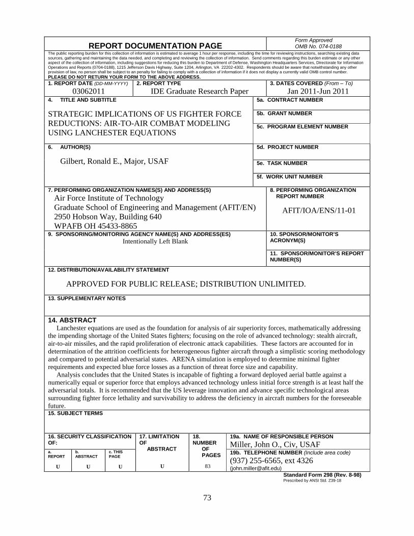
73
REPORT DOCUMENTATION PAGE Form Approved OMB No. 074-0188
The public reporting burden for this collection of information is estimated to average 1 hour per response, including the time for reviewing instructions, searching existing data sources, gathering and maintaining the data needed, and completing and reviewing the collection of information. Send comments regarding this burden estimate or any other aspect of the collection of information, including suggestions for reducing this burden to Department of Defense, Washington Headquarters Services, Directorate for Information Operations and Reports (0704-0188), 1215 Jefferson Davis Highway, Suite 1204, Arlington, VA 22202-4302. Respondents should be aware that notwithstanding any other provision of law, no person shall be subject to an penalty for failing to comply with a collection of information if it does not display a currently valid OMB control number. PLEASE DO NOT RETURN YOUR FORM TO THE ABOVE ADDRESS. 1. REPORT DATE (DD-MM-YYYY)
03062011 2. REPORT TYPE
IDE Graduate Research Paper 3. DATES COVERED (From – To)
Jan 2011-Jun 2011 4. TITLE AND SUBTITLE STRATEGIC IMPLICATIONS OF US FIGHTER FORCE REDUCTIONS: AIR-TO-AIR COMBAT MODELING USING LANCHESTER EQUATIONS
5a. CONTRACT NUMBER
5b. GRANT NUMBER 5c. PROGRAM ELEMENT NUMBER
6. AUTHOR(S) Gilbert, Ronald E., Major, USAF
5d. PROJECT NUMBER 5e. TASK NUMBER
5f. WORK UNIT NUMBER
7. PERFORMING ORGANIZATION NAMES(S) AND ADDRESS(S) Air Force Institute of Technology Graduate School of Engineering and Management (AFIT/EN) 2950 Hobson Way, Building 640 WPAFB OH 45433-8865
8. PERFORMING ORGANIZATION REPORT NUMBER AFIT/IOA/ENS/11-01
9. SPONSORING/MONITORING AGENCY NAME(S) AND ADDRESS(ES) Intentionally Left Blank
10. SPONSOR/MONITOR’S ACRONYM(S) 11. SPONSOR/MONITOR’S REPORT NUMBER(S)
12. DISTRIBUTION/AVAILABILITY STATEMENT APPROVED FOR PUBLIC RELEASE; DISTRIBUTION UNLIMITED.
13. SUPPLEMENTARY NOTES
14. ABSTRACT Lanchester equations are used as the foundation for analysis of air superiority forces, mathematically addressing the impending shortage of the United States fighters; focusing on the role of advanced technology: stealth aircraft, air-to-air missiles, and the rapid proliferation of electronic attack capabilities. These factors are accounted for in determination of the attrition coefficients for heterogeneous fighter aircraft through a simplistic scoring methodology and compared to potential adversarial states. ARENA simulation is employed to determine minimal fighter requirements and expected blue force losses as a function of threat force size and capability. Analysis concludes that the United States is incapable of fighting a forward deployed aerial battle against a numerically equal or superior force that employs advanced technology unless initial force strength is at least half the adversarial totals. It is recommended that the US leverage innovation and advance specific technological areas surrounding fighter force lethality and survivability to address the deficiency in aircraft numbers for the foreseeable future. 15. SUBJECT TERMS
16. SECURITY CLASSIFICATION OF:
17. LIMITATION OF ABSTRACT
U
18. NUMBER OF PAGES
83
19a. NAME OF RESPONSIBLE PERSON Miller, John O., Civ, USAF
a. REPORT
U
b. ABSTRACT
U
c. THIS PAGE
U
19b. TELEPHONE NUMBER (Include area code) (937) 255-6565, ext 4326 ([email protected])
Standard Form 298 (Rev. 8-98) Prescribed by ANSI Std. Z39-18

74