Storm Surges, Informational Shocks, and the Price of Urban ......Storm Surges, Informational Shocks,...

1

Storm Surges, Informational Shocks, and the Price of Urban Real Estate:

An Application to the Case of Hurricane Sandy*

Jason Barr

Department of Economics

Rutgers University-Newark

Email: [email protected]

Jeffrey P. Cohen

Center for Real Estate

Department of Finance

School of Business

University of Connecticut


Eon Kim

Department of Security and Crime Science

University College of London


September 2017

Abstract: The impacts of a major hurricane on commercial and residential real estate can be

devastating. Recent events in Houston (with Hurricane Harvey), Florida (with Hurricane Irma),

and New York City (with Hurricane Sandy) are examples of how flooding damage can

unexpectedly extend beyond the FEMA flood zones. Such surprises or shocks can provide

property owners—including those that are not flooded—with new information about future flood

risks, based on the difference of the property distance from the flood zone and the distance to the

actual locations of flooding. We apply a new estimation strategy to quantify the effects of these

shocks on property values, using information on repeat property sales to estimate a separate

shock effect for each dry property. We demonstrate our approach with an application to non-

flooded properties in New York City for Hurricane Sandy. We find that, in general, houses,

apartments and commercial properties show the most price volatility within the older, denser

urban core, mostly in those neighborhoods that appear to be gentrifying.

Key words: Hurricane Sandy, Storm Surges, New York City, Locally Weighted Regressions,

Real Estate Prices

JEL Classification: R3, C14

*We would like to thank the National Resources Defense Council for providing GIS maps related to Hurricane

Sandy. Earlier versions of the paper were presented at the 2017 AREUEA National Conference and the 2017

Eastern Economics Association meetings. We thank Steve Malpezzi, Suleyman Taspinar and session participants for

their comments. Any errors belong to the authors.

mailto:[email protected]



2

1. Introduction

Recent hurricanes in the U.S., including 2017 in Houston (with Hurricane Harvey) and Florida

(with Irma), and 2012 in New York City (with Hurricane Sandy) are examples of how flooding

damage can unexpectedly extend beyond the Federal Emergency Management Agency (FEMA)

designated flood zones.1 Such surprises or shocks can provide property owners—including those

that were not flooded—with new information about future flood risks, based on the difference

between the distance of their properties from the flood zone and the distance to the actual

locations of flooding. We apply a new estimation strategy to quantify the effects of these shocks

on property values for non-flooded properties. One of the innovations in our approach is that we

use information on repeat property sales to estimate a separate shock effect for each dry property.

Using locally weighted regressions (LWRs), we investigate the heterogeneous effects across the

city. Our approach also addresses both demand effects and supply effects from the storm and

possible sample selection.

We demonstrate our approach with an application to non-flooded properties in New York City

for repeat sales that sold once before and again after Sandy. We find that, in general, houses,

apartments and commercial properties showed the most volatility within the older, denser urban

core, mostly in those neighborhoods that appear to be gentrifying. We also perform falsification

tests to validate our identification strategy for the Sandy application.

With respect to specific hurricanes, Harvey struck the Houston, Texas area in late-August 2017.

The preliminary damage assessment is in the range of $150 billion (McWilliams and Marianna,

2017), with thousands of houses destroyed and many more properties, both residential and

commercial, sustaining major damage. In early September 2017, Hurricane Irma hit Florida, with

waist-deep flooding in downtown Miami (Sun-Sentinel, 2017), among other areas of the state.

The total costs of Irma could reach as high as $300 billion (Wood, 2017).2 On a somewhat

smaller but, nevertheless dramatic, scale, on October 29, 2012, Hurricane Sandy made landfall in

New York City; it was arguably the largest and most damaging storm to hit the New York

metropolitan region. 65 deaths in New York, New Jersey and Connecticut were tied to the storm.

The surge level at Battery Park in lower Manhattan topped out at 13.88 feet at 9:24 pm,

surpassing the old record of 10.02 feet, set by Hurricane Donna in 1960 (CNN, 2013). Estimates

of total losses for New York City alone were about $19 billion, and $33 billion for the entire

state.3

Studies to date have focused on estimating the cost of the damage—how much did the storm

destroy in terms of market value or the replacement costs (ESA, 2013). However, to our

knowledge, no work has explored the implicit costs of storm surges on the value of real estate in

the city for properties that were not damaged by the surge. Understanding how the flooding

affected the properties that remained dry is important because it can give clues to how the market

1 For Harvey see: https://www.nytimes.com/interactive/2017/09/01/us/houston-damaged-buildings-in-fema-flood-

zones.html?mcubz=1&_r=1. 2 At the time of writing this paper, the damage totals from Irma had still been under assessment. 3 For New York City see:

http://www.nyc.gov/html/sirr/downloads/pdf/final_report/Ch_1_SandyImpacts_FINAL_singles.pdf.

https://www.nytimes.com/interactive/2017/09/01/us/houston-damaged-buildings-in-fema-flood-zones.html?mcubz=1&_r=1


http://www.nyc.gov/html/sirr/downloads/pdf/final_report/Ch_1_SandyImpacts_FINAL_singles.pdf

3

perceives the future risks of storm surges that are likely to occur more frequently over time.

Which neighborhoods reacted the most and why? This paper develops a new methodology to

investigate real estate price volatility due to relative beliefs or expectations about future surges,

buy focusing on changes in real estate prices for those properties not directly flooded.

In 1968, Congress created the National Flood Insurance Program (NFIP) to help provide a means

for property owners to financially protect themselves. The NFIP offers flood insurance to

homeowners, renters, and business owners if their respective town or city participates in the

NFIP. Participating communities agree to adopt and enforce ordinances that meet or exceed

Federal Emergency Management Agency (FEMA) requirements to reduce the risk of flooding

(FEMA, 2017b)

FEMA partners with states and communities through the Risk Mapping, Assessment, and

Planning (Risk MAP) program to identify flood hazards and assess flood risks. These data are

incorporated into flood maps, known as Flood Insurance Rate Maps (FIRMs), which support the

NFIP and provide the basis for community floodplain management regulations and flood

insurance requirements. Most commonly used for insurance purposes are the 100-year floodplain

maps, which are regions designated to have a 1% chance of being inundated each year.

Real estate buyers, who seek a mortgage, are often required to purchase flood insurance if they

are within a FEMA-designated floodplain (FEMA, 2017a). The FEMA floodplain maps thus

serve as a publicly available assessment of the likelihood of a property being flooded. In

addition, for those outside the floodplain, the distance to the plain can presumably be used to

provide information about the relative flood safety of the neighborhood. Being 20 feet from a

floodplain suggests that a property is potentially at more risk than one 2,000 feet away.

While it is relatively straightforward to estimate the effects of the storm on those properties that

were flooded by a major storm, our main goal is to estimate the degree to which properties that

remained dry may or may not be impacted by a storm. If the Hurricane represents an

informational shock about the likelihood of future damage then, presumably, this effect will be

priced into properties, as people reassess the likelihood of future storm shocks and the potential

damage they could cause.

Because real estate in a city is often a form of urban system, the effects of property value

changes on one neighborhood are not independent of the markets in surrounding neighborhoods.

Measuring average effects or even using neighborhood-dummies do not control for or measure

the locational interdependencies across a city. For instance, with Sandy, the farthest property

away from the surge was only three miles; most parts of the city are relatively low lying. So, in

theory, vast swaths of the city could be susceptible to future surges.

This paper employs several relatively new and important empirical strategies to isolate the

expectations of the real estate market. First we focus on repeat sales (though we also include

hedonic regressions) to eliminate measurement problems due to unobservable static features of

the structure (be they related to the quality of the structure, or neighborhood features). Second,

for each neighborhood (or in the specific case of New York City, each borough), we estimate

4

changes in the average prices over time to control for market-wide fluctuations independent of

the storm surge; the index is derived based on sales that took place only before or only after a

hurricane. Again, because we are focusing on those properties not damaged by the storm surge,

repeat sales are an appropriate and an important method to estimate the non-direct impact of the

hurricane.

Next, we employ locally weighted regressions (LWRs), as in (Cleveland and Devlin, 1988).

Because ordinarily least squares (OLS) estimates are not likely to capture the possible

heterogeneity in how the market price of properties responded across neighborhoods, we develop

the repeat sales approach using the method of locally weighted regressions (LWRs) in order to

determine whether there are different coefficient estimates for each property in the sample. If

price volatility effects across a city were uniform, we would not reject the null hypothesis of

uniform coefficients across the city. In our specific application of New York City, our tests on

the sample of repeat sales properties reject this null hypothesis and suggest that while the price of

many dry properties across the city were not significantly affected by the storm, others did see

price effects due to the storm. The LWR method allows us to explore heterogeneous effects for

each property in the sample, and how and why prices changed (or not) for each property.

Thus, this paper contributes not only to our understanding of how storms affect real estate

values, but also demonstrates that these effects often can be heterogeneous. Two buildings that

are similar in their age, use, and quality, and were the same distance from the storm surge, can,

in fact, be impacted by the storm differently, based on the economic and demographic profile of

the neighborhoods, for example. We want to stress that a difference-in-differences model to

determine the impact of the storm does not allow for the type of heterogeneity we are looking to

uncover. OLS coefficient estimates represent averages for an entire city, and by focusing only

the average effects, one may “throw out the baby with the bath water.” That is to say, when

investigating the geographic impacts of storms and/or other shocks to cities, it is vital to

understand the variation in these impacts; this is crucial not only for measurement reasons but for

the policy implications about where to deploy resources before or after a storm.

In regard to our data set for the Sandy application, we first collected a very large data set for

New York City on nearly all open market transactions for all properties before and after Sandy,

which runs from January 2003 to October 2014, where Sandy made landfall in New York and

New Jersey on October 29, 2012. We thus have transactions for nearly all types of property in

the city, not just single-family homes. We then merged this data set with geographic information

about whether each property was in the FEMA 100-year floodplain or not, whether it was in the

storm surge zone or not, and how far each property was to both the FEMA floodplain map and

the storm surge boundaries, respectively. Additional controls include the property elevation,

distance to the shoreline, and characteristics about the property and its location.

Using LWRs for three different property classes (one and two family homes, apartment

buildings, and commercial properties),4 we find significant variation in price change responses to

the storm surge. In Staten Island and the Bronx, we find relatively less reaction to the storm,

4 See Appendix A for information about the data set. The commercial properties include offices, retail, factories,

lofts, hospitals, and a few other types.

5

while in Queens and Brooklyn we find strong price reactions to the surge (relative to the FEMA

line). The price effects for Manhattan are weak for one and two family homes (of which there are

relatively few) but stronger for apartments buildings and commercial properties.

As to the question of what is driving the variation, we regress the LWR coefficients on several

control variables, using OLS. We find that for each type of property, distance to the city center

(the Empire State Building) is a strongly negative predictor of shock responses. In other words,

across property types the responses to the surge were much greater closer to the center, all else

equal. We also find evidence that census tracts with better subway access and higher incomes

(for homes and offices) were also more responsive to the “shocks.” We infer that this likely to be

due to gentrification and the rising value the residents are placing on being close to the city

center. That is to say, it is likely that the people moving into center with higher incomes might

be more responsive to these shocks, ceteris paribus.

The remainder of this paper proceeds as follows. The next section provides a literature review on

the effects of storms and storm surges on real estate prices. Then Section 3 provides the

background on our methodology that informs the statistical analysis. Section 4 provides

information on the data set for the Hurricane Sandy application. Sections 5 and 6 provides

evidence on the effects of the storm surge on both flooded non-flooded properties throughout the

city, using hedonic regressions and LWRs, respectively. In Section 7, we test for reasons why

there were heterogeneous effects across the city. Section 8 performs robustness checks for the

LWR results. Finally, Section 9 offers some concluding remarks. Appendix A provides

information about data sources, processing, and additional results, while Appendix B consists of

some background information about LWRs. Finally, Appendix C contains background

information for the data and procedures used in Section 7 of the paper.

2. Literature Review

The recent events of Hurricane Harvey in Texas and Irma in Florida demonstrate that the FEMA

flood zones remain an imperfect measure of flooding likelihoods (Fessenden, et al., 2017).

However, it is far too soon for an econometric study of the impacts on real estate values.

Therefore, we focus our review on hurricanes that occurred several years ago.

There are a variety of studies that investigate the impacts of storms or natural disaster on real

estate and local economies. These include studies of specific hurricanes, as well as others the

proximity to the coast or flood risks. One recent study focuses on New York City housing prices

and Hurricane Sandy. Specifically, Ortega and Taspinar (2016) examine Sandy and the New

York City housing market, and address the question of whether housing demand shifted towards

less exposed areas. They divide the City into 6 Hurricane Evacuation Zones (HEZ’s). They allow

for “treatments” of 0 (no damage), 1 (minor damage), and 2 (major damage), and compare prices

post-Sandy for the treatment vs. control groups.

Their difference-in-differences model includes a dependent variable of the log of house sales

prices, and they include a dummy for post-Sandy sales for being in zones 1 or 2, and

6

neighborhood and time fixed effects. They also estimate a second difference-in-differences

model with all three treatment groups, each of which is interacted with a post-Sandy dummy

variable. They find evidence that the treatment effects are significant. They also consider

whether or not there is a sample selection bias because they only examine properties that have

sold, by using assessment data that encompass all residential properties in the city. They find

little evidence of this type of sample selection. They also find that for damaged houses, the

treatment effects appear to be permanent.

Bin and Landry (2013), in contrast, find that the effects of unexpected flood risk following a

major storm disappear after several years. They examine Pitt County, North Carolina and find a

discount of between 5% and 9% following Hurricanes Fran and Floyd. More recent data indicate

a higher discount rate, although as noted above, these effects vanish as additional time elapses.

Bin et al. (2011) focus on a similar geographic area in North Carolina to estimate an approximate

value of lost property due to potential flooding in these areas. For a 20 to 70 year period into the

future, they forecast between a $179 million and $576 million loss for properties in four counties

near the shore in North Carolina.

In another coastal study, Atreya and Czajkowski (2016) use a spatial hedonic model to study the

price effects of proximity to the coast in Galveston, Texas. They find that with ¼ mile from the

coast, properties sell for higher prices than those that are further away. An earlier study in this

literature is MacDonald, Murdoch and White (1987), who estimate a hedonic house price

function to study Monroe, Louisiana, an area prone to flooding. Given the nonlinear functional

form for the dependent variable (i.e., the sales price), it is not straightforward in general to

indicate one magnitude and direction for the marginal effects, but these effects depend on the

fitted values of each of the sales prices. They provide a few examples of the effects for a small

sample of homes, and they find that for these houses a higher flood risk leads to a decrease in

sales prices in the range of $2000 to $8000.

Examining the impacts of a hurricane as a natural experiment extends beyond the literature on

real estate impacts. Gallagher and Hartley (forthcoming) study how household debt is impacted

by Hurricane Katrina, and they find that more flooding result in lower amounts of total debt,

which is primarily due to less home mortgage debt. Kocornik-Mina et al. (2015) study the

impacts of floods on economic activity in cities in 40 countries throughout the world. They

utilize data on city night lights to estimate economic activity. They find that more well-

established cities tend to bounce back in terms of economic activity following major floods that

displace large numbers of residents, while more recently developed cities tend to see declines in

economic activity that persist following major flooding.

Finally, Meltzer and Ellen (2017) investigate the impact of Hurricane Sandy on small businesses

vulnerability in New York City by looking at firms and employment before and after the storm.

Their regression results show significant post-Sandy job declines, of about 4.5 to 6 per census

block, for the retail sector only. But, across all job types, the impacts from Sandy are noisy and

largely insignificant.

7

With these studies in mind, we now turn to our new methodology to estimate the impacts on dry

properties.

3. The Theory of Price Effects

While we do not deny that it is important to understand how storms affect the properties hit by

the storm surges or hurricanes, our aim is to understand how a storm shock can affect those

properties that were not damaged by the storm. The point is that for many property owners the

storm represented new information on the potential damage due to storm surges. A priori,

however, the effects of a storm on the dry side of the storm surge can be unclear. On the one

hand, the surge was a negative shock to the city, and, as a result, it represents the possibility that

the city is subject to future surges. Those property owners relatively close to the surge are

particularly vulnerable. This can be called the demand effect, where a negative neighborhood

shock would reduce the demand for real estate and thus reduce its price.

On the other hand, there are likely to be supply effects. First, properties in the flooded zone were

damaged or destroyed, which would reduce the quantity and quality of available real estate in a

particular neighborhood; this would have the effect of making the remaining structures close by

relatively more valuable. There are also likely to be second order effects of shifting demand from

the wet part to dry part. If properties in “gentrifying” neighborhoods experience a loss of real

estate due to the surge, but the neighborhood remains in strong demand overall, then the relative

demand within a neighborhood might positively shift to the dry properties. Thus, the dry

properties may receive two benefits that could raise their prices—the relative scarcity of

structures in a neighborhood near the flood will increase their price, and shifting relative demand

within the neighborhood could also drive up the prices of dry properties.

Our main identification strategy is to look at the informational shock that occurred based on the

FEMA floodplain maps used to assess insurance premiums. In short, our variable of interest is

the difference between the closest distance of a property to the FEMA floodplain relative to the

closest distance to the storm surge.

That is, we aim to estimate:

∆𝑙𝑛𝑃𝑖 = 𝜃𝑠ℎ𝑜𝑐𝑘𝑖 + 𝑋𝑖휁+ε𝑖

where

𝑠ℎ𝑜𝑐𝑘𝑖 = 𝑠𝑢𝑟𝑔𝑒 𝑑𝑖𝑠𝑡𝑎𝑛𝑐𝑒𝑖 − 𝐹𝐸𝑀𝐴 𝑓𝑙𝑜𝑜𝑑𝑝𝑙𝑎𝑖𝑛 𝑑𝑖𝑠𝑡𝑎𝑛𝑐𝑒𝑖

for 𝑖 = 1, … , 𝑁, non-flooded properties, and where 𝑋𝑖 are control variables and ε𝑖 is the error

term. ∆𝑙𝑛𝑃𝑖 is the price change given that the first sale is before the storm and the second sale is

after the storm, i.e., where repeat sales straddle the storm.

As an example, take two identical houses, A and B, where each is say 100 feet from the closest

FEMA floodplain boundary line. For house A, say the flood approached within 150 feet, for a

𝑠ℎ𝑜𝑐𝑘 = 150 − 100 = 50 (so that any value above 0 is “good news” or a positive shock). In the

case of house B, say the flood came to within 50 feet of the house, for a 𝑠ℎ𝑜𝑐𝑘 = 50 − 100 =

8

−50; thus a negative shock. In this case, we would expect house B to lose value, relative to

house A. This would then suggest that 𝜃 > 0, where 𝜃 is the effect of a one foot shock on the

housing price change.

In order to estimate 𝜃, we employ several different empirical strategies. First, we use hedonic

regressions to estimate the impacts on the dry and wet sides; for this we use difference-in-

difference measures. But, because of the size of the data set, we are able to use repeat sales that

allow us to “net out” the static unobservable characteristics that might otherwise be omitted. To

this end, we use a technique similar to Ries and Somerville (2010), where we first estimate a

price index to estimate price-effects that are independent of the storm. We also include a measure

of 2010 census tract building occupancy rate changes to control for supply effects (both because

of, and independent of, the storm). As described below, we are able to measure the changes in

the occupancies rates before and after the storm using vacancy data provided by the Department

of Housing and Urban Development (HUD), and thus our estimation is able to measure the

demand effect—how much of prices changes were due to informational shocks, rather than

changes in the real estate stock.

A key issue, however, is not just whether 𝜃 > 0, but whether the magnitude of 𝜃 varies across

the city. Are their spatial differences in how responsive some properties are to the size (and sign)

of the shock? If so, this would suggest that OLS estimators are not fully capturing the degree of

spatial variation in the shocks. For this reason we employ locally weighted regressions (LWRs)

(described below), which gives an estimate, 𝜃𝑖, for each property in the sample. Given the

complexity of many cities, their heterogeneous demographics, and diverse real estate stock, there

is no reason to believe, a priori, that the effects of a storm on the dry side were homogenous;

rather prices in different neighborhoods are likely to respond differently based on the perceived

risk and the characteristics of those residents who do the perceiving, as it were.

3.1 Methodology

Each period, properties owners have information about the likelihood of flooding affecting their

property, i. Denote,

𝐹𝑖𝑡 = 𝑓𝑙𝑜𝑜𝑑𝑖𝑛𝑔 𝑙𝑖𝑘𝑒𝑙𝑖ℎ𝑜𝑜𝑑 𝑒𝑠𝑡𝑖𝑚𝑎𝑡𝑒𝑖𝑡,

for each period t. If t is before October 29, 2012, then

𝐹𝑖𝑡 = 𝑑𝑖𝑠𝑡𝑎𝑛𝑐𝑒 𝑡𝑜 𝐹𝐸𝑀𝐴 𝑓𝑙𝑜𝑜𝑑𝑝𝑙𝑎𝑖𝑛 𝑚𝑎𝑝𝑖𝑡

If t is after the storm (denote this then t+j),

𝐹𝑖𝑡+𝑗 = 𝑑𝑖𝑠𝑡𝑎𝑛𝑐𝑒 𝑡𝑜 𝑆𝑎𝑛𝑑𝑦 𝑖𝑛𝑢𝑛𝑑𝑎𝑡𝑖𝑜𝑛 𝑏𝑜𝑢𝑛𝑑𝑎𝑟𝑦𝑖𝑡+𝑗

In order to estimate the informational shock from the storm, we examine repeat sales properties

that sold once before Sandy (in time t), and once again after Sandy (in time t+j). The objective is

to use Sandy as a “natural experiment” to identify the effects on property prices in changes in the

likelihood of storm-related flooding.

Because neighborhood-level price changes, in principle, can be correlated with the changes in

distances to flood zones, an identification strategy is necessary to avoid potential biases that

9

could arise because of the correlation between the neighborhood price level movement and the

flood zone distances.

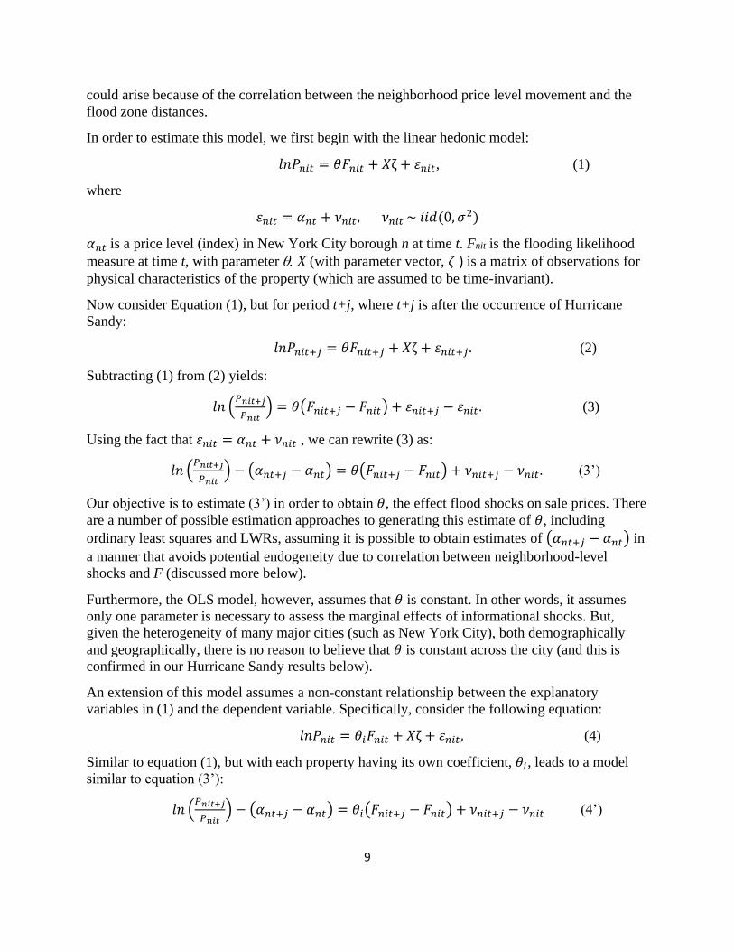
In order to estimate this model, we first begin with the linear hedonic model:

𝑙𝑛𝑃𝑛𝑖𝑡 = 𝜃𝐹𝑛𝑖𝑡 + 𝑋ζ + 휀𝑛𝑖𝑡, (1)

where

휀𝑛𝑖𝑡 = 𝛼𝑛𝑡 + 𝜈𝑛𝑖𝑡, 𝜈𝑛𝑖𝑡 ~ 𝑖𝑖𝑑(0, 𝜎2)

𝛼𝑛𝑡 is a price level (index) in New York City borough n at time t. Fnit is the flooding likelihood

measure at time t, with parameter X (with parameter vector, 휁) is a matrix of observations for

physical characteristics of the property (which are assumed to be time-invariant).

Now consider Equation (1), but for period t+j, where t+j is after the occurrence of Hurricane

Sandy:

𝑙𝑛𝑃𝑛𝑖𝑡+𝑗 = 𝜃𝐹𝑛𝑖𝑡+𝑗 + 𝑋ζ + 휀𝑛𝑖𝑡+𝑗 . (2)

Subtracting (1) from (2) yields:

𝑙𝑛 (𝑃𝑛𝑖𝑡+𝑗

𝑃𝑛𝑖𝑡) = 𝜃(𝐹𝑛𝑖𝑡+𝑗 − 𝐹𝑛𝑖𝑡) + 휀𝑛𝑖𝑡+𝑗 − 휀𝑛𝑖𝑡 . (3)

Using the fact that 휀𝑛𝑖𝑡 = 𝛼𝑛𝑡 + 𝜈𝑛𝑖𝑡 , we can rewrite (3) as:


𝑃𝑛𝑖𝑡) − (𝛼𝑛𝑡+𝑗 − 𝛼𝑛𝑡) = 𝜃(𝐹𝑛𝑖𝑡+𝑗 − 𝐹𝑛𝑖𝑡) + 𝜈𝑛𝑖𝑡+𝑗 − 𝜈𝑛𝑖𝑡. (3’)

Our objective is to estimate (3’) in order to obtain 𝜃, the effect flood shocks on sale prices. There

are a number of possible estimation approaches to generating this estimate of 𝜃, including

ordinary least squares and LWRs, assuming it is possible to obtain estimates of (𝛼𝑛𝑡+𝑗 − 𝛼𝑛𝑡) in

a manner that avoids potential endogeneity due to correlation between neighborhood-level

shocks and F (discussed more below).

Furthermore, the OLS model, however, assumes that 𝜃 is constant. In other words, it assumes

only one parameter is necessary to assess the marginal effects of informational shocks. But,

given the heterogeneity of many major cities (such as New York City), both demographically

and geographically, there is no reason to believe that 𝜃 is constant across the city (and this is

confirmed in our Hurricane Sandy results below).

An extension of this model assumes a non-constant relationship between the explanatory

variables in (1) and the dependent variable. Specifically, consider the following equation:

𝑙𝑛𝑃𝑛𝑖𝑡 = 𝜃𝑖𝐹𝑛𝑖𝑡 + 𝑋ζ + 휀𝑛𝑖𝑡 , (4)

Similar to equation (1), but with each property having its own coefficient, 𝜃𝑖, leads to a model

similar to equation (3’):


𝑃𝑛𝑖𝑡) − (𝛼𝑛𝑡+𝑗 − 𝛼𝑛𝑡) = 𝜃𝑖(𝐹𝑛𝑖𝑡+𝑗 − 𝐹𝑛𝑖𝑡) + 𝜈𝑛𝑖𝑡+𝑗 − 𝜈𝑛𝑖𝑡 (4’)

10

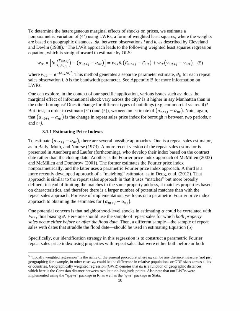
To determine the heterogeneous marginal effects of shocks on prices, we estimate a

nonparametric variation of (4’) using LWRs, a form of weighted least squares, where the weights

are based on geographic distances, dik, between observations i and k, as described by Cleveland

and Devlin (1988). 5 The LWR approach leads to the following weighted least squares regression

equation, which is straightforward to estimate by OLS:

𝑤𝑖𝑘 × [𝑙𝑛 (𝑃𝑛𝑖𝑡+𝑗

𝑃𝑛𝑖𝑡) − (𝛼𝑛𝑡+𝑗 − 𝛼𝑛𝑡)] = 𝑤𝑖𝑘𝜃𝑖(𝐹𝑛𝑖𝑡+𝑗 − 𝐹𝑛𝑖𝑡) + 𝑤𝑖𝑘(𝜈𝑛𝑖𝑡+𝑗 − 𝜈𝑛𝑖𝑡) (5)

where 𝑤𝑖𝑘 = 𝑒−(𝑑𝑖𝑘/𝑏)2. This method generates a separate parameter estimate, 𝜃𝑖, for each repeat

sales observation i. b is the bandwidth parameter. See Appendix B for more information on

LWRs.

One can explore, in the context of our specific application, various issues such as: does the

marginal effect of informational shock vary across the city? Is it higher in say Manhattan than in

the other boroughs? Does it change for different types of buildings (e.g. commercial vs. retail)?

But first, in order to estimate (3’) (and (5)), we need an estimate of (𝛼𝑛𝑡+𝑗 − 𝛼𝑛𝑡). Note, again,

that (𝛼𝑛𝑡+𝑗 − 𝛼𝑛𝑡) is the change in repeat sales price index for borough n between two periods, t

and t+j.

3.1.1 Estimating Price Indexes

To estimate (𝛼𝑛𝑡+𝑗 − 𝛼𝑛𝑡), there are several possible approaches. One is a repeat sales estimator,

as in Baily, Muth, and Nourse (1973). A more recent version of the repeat sales estimator is

presented in Anenberg and Laufer (forthcoming), who develop their index based on the contract

date rather than the closing date. Another is the Fourier price index approach of McMillen (2003)

and McMillen and Dombrow (2001). The former estimates the Fourier price index

nonparametrically, and the latter uses a parametric Fourier price index approach. A third is a

more recently developed approach of a “matching” estimator, as in Deng, et al. (2012). That

approach is similar to the repeat sales approach in that it uses “matches” but more broadly

defined; instead of limiting the matches to the same property address, it matches properties based

on characteristics, and therefore there is a larger number of potential matches than with the

repeat sales approach. For ease of implementation, we focus on a parametric Fourier price index

approach to obtaining the estimates for (𝛼𝑛𝑡+𝑗 − 𝛼𝑛𝑡).

One potential concern is that neighborhood-level shocks in estimating could be correlated with

Fni,t , thus biasing 𝜃. Here one should use the sample of repeat sales for which both property

sales occur either before or after the flood date. Then, a different sample—the sample of repeat

sales with dates that straddle the flood date—should be used in estimating Equation (5).

Specifically, our identification strategy in this regression is to construct a parametric Fourier

repeat sales price index using properties with repeat sales that were either both before or both

5 “Locally weighted regression” is the name of the general procedure where dik can be any distance measure (not just

geographic); for example, in other cases dik could be the difference in relative populations or GDP sizes across cities

or countries. Geographically weighted regression (GWR) denotes that dik is a function of geographic distances,

which here is the Cartesian distance between two latitude-longitude points. Also note that our LWRs were

implemented using the “spgwr” package in R, as well as the “gwr” package in Stata.

11

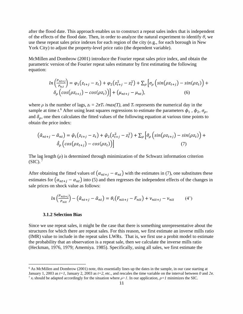
after the flood date. This approach enables us to construct a repeat sales index that is independent

of the effects of the flood date. Then, in order to analyze the natural experiment to identify θ, we

use these repeat sales price indexes for each region of the city (e.g., for each borough in New

York City) to adjust the property-level price ratio (the dependent variable).

McMillen and Dombrow (2001) introduce the Fourier repeat sales price index, and obtain the

parametric version of the Fourier repeat sales estimator by first estimating the following

equation:

𝑙𝑛 (𝑃𝑛𝑡+𝑗

𝑃𝑛,𝑡) = 𝜑1(𝑧𝑡+𝑗 − 𝑧𝑡) + 𝜑2(𝑧𝑡+𝑗

2 − 𝑧𝑡2) + ∑ [𝜎𝜌 (𝑠𝑖𝑛(𝜌𝑧𝑡+𝑗) − 𝑠𝑖𝑛(𝜌𝑧𝑡)) +𝜌

𝛿𝜌 (𝑐𝑜𝑠(𝜌𝑧𝑡+𝑗) − 𝑐𝑜𝑠(𝜌𝑧𝑡))] + (𝜇𝑛𝑡+𝑗 − 𝜇𝑛𝑡), (6)

where ρ is the number of lags, zt = 2πTt /max(T), and Tt represents the numerical day in the

sample at time t.6 After using least squares regressions to estimate the parameters 𝜙1 , 𝜙2, 𝜎𝜌,

and 𝛿𝜌, one then calculates the fitted values of the following equation at various time points to

obtain the price index:

(�̂�𝑛𝑡+𝑗 − �̂�𝑛𝑡) = �̂�1(𝑧𝑡+𝑗 − 𝑧𝑡) + �̂�2(𝑧𝑡+𝑗2 − 𝑧𝑡

2) + ∑ [�̂�𝜌 (𝑠𝑖𝑛(𝜌𝑧𝑡+𝑗) − 𝑠𝑖𝑛(𝜌𝑧𝑡)) +𝜌

�̂�𝜌 (𝑐𝑜𝑠(𝜌𝑧𝑡+𝑗) − 𝑐𝑜𝑠(𝜌𝑧𝑡))] (7)

The lag length (ρ) is determined through minimization of the Schwarz information criterion

(SIC). 7

After obtaining the fitted values of (𝛼𝑛𝑡+𝑗 − 𝛼𝑛𝑡) with the estimates in (7), one substitutes these

estimates for (𝛼𝑛𝑡+𝑗 − 𝛼𝑛𝑡) into (5) and then regresses the independent effects of the changes in

sale prices on shock value as follows:


𝑃𝑛𝑖𝑡) − (�̂�𝑛𝑡+𝑗 − �̂�𝑛𝑡) = 𝜃𝑖(𝐹𝑛𝑖𝑡+𝑗 − 𝐹𝑛𝑖𝑡) + 𝜈𝑛𝑖𝑡+𝑗 − 𝜈𝑛𝑖𝑡 (4’)

3.1.2 Selection Bias

Since we use repeat sales, it might be the case that there is something unrepresentative about the

structures for which there are repeat sales. For this reason, we first estimate an inverse mills ratio

(IMR) value to include in the repeat sales LWRs. That is, we first use a probit model to estimate

the probability that an observation is a repeat sale, then we calculate the inverse mills ratio

(Heckman, 1976, 1979; Amemiya. 1985). Specifically, using all sales, we first estimate the

6 As McMillen and Dombrow (2001) note, this essentially lines up the dates in the sample, in our case starting at

January 1, 2003 as t=1, January 2, 2003 as t=2, etc., and rescales the time variable on the interval between 0 and 2π. 7 xi should be adapted accordingly for the situation where ρ>1. In our application, 𝜌=1 minimizes the SIC.

12

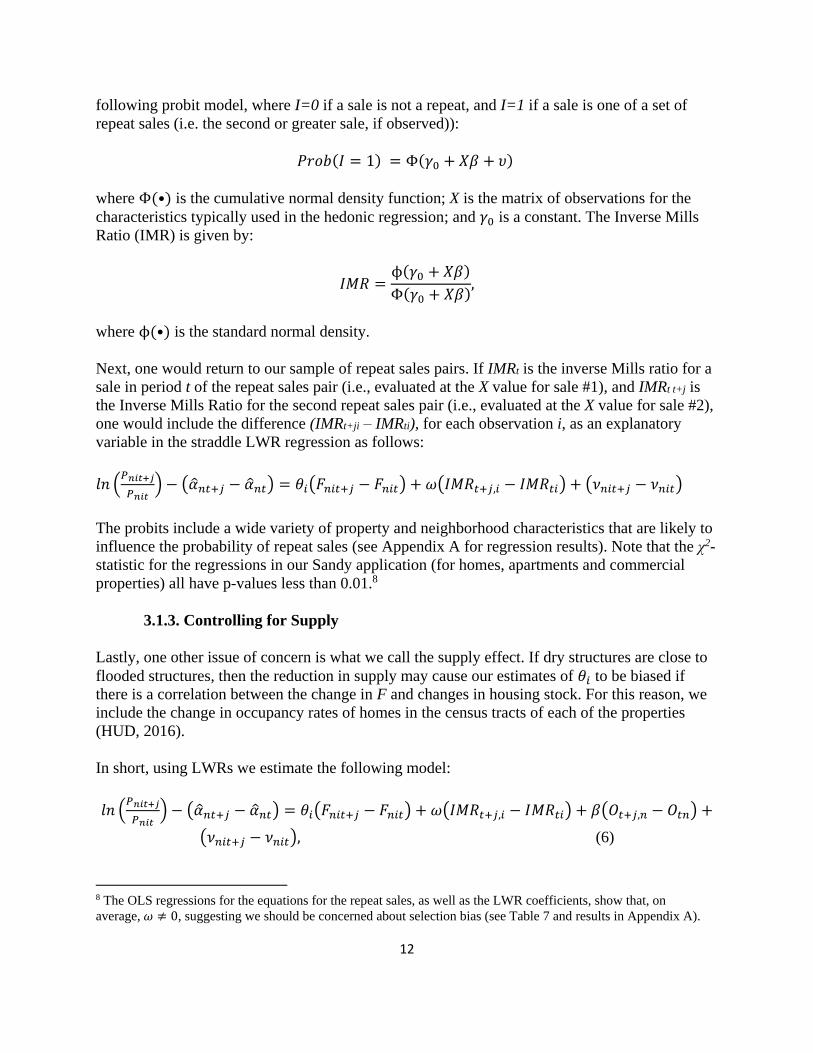
following probit model, where I=0 if a sale is not a repeat, and I=1 if a sale is one of a set of

repeat sales (i.e. the second or greater sale, if observed)):

𝑃𝑟𝑜𝑏(𝐼 = 1) = Φ(𝛾0 + 𝑋𝛽 + 𝜐)

where Φ(•) is the cumulative normal density function; X is the matrix of observations for the

characteristics typically used in the hedonic regression; and 𝛾0 is a constant. The Inverse Mills

Ratio (IMR) is given by:

𝐼𝑀𝑅 =ϕ(𝛾0 + 𝑋𝛽)

Φ(𝛾0 + 𝑋𝛽),

where ϕ(•) is the standard normal density.

Next, one would return to our sample of repeat sales pairs. If IMRt is the inverse Mills ratio for a

sale in period t of the repeat sales pair (i.e., evaluated at the X value for sale #1), and IMRt t+j is

the Inverse Mills Ratio for the second repeat sales pair (i.e., evaluated at the X value for sale #2),

one would include the difference (IMRt+ji – IMRti), for each observation i, as an explanatory

variable in the straddle LWR regression as follows:


𝑃𝑛𝑖𝑡) − (�̂�𝑛𝑡+𝑗 − �̂�𝑛𝑡) = 𝜃𝑖(𝐹𝑛𝑖𝑡+𝑗 − 𝐹𝑛𝑖𝑡) + 𝜔(𝐼𝑀𝑅𝑡+𝑗,𝑖 − 𝐼𝑀𝑅𝑡𝑖) + (𝜈𝑛𝑖𝑡+𝑗 − 𝜈𝑛𝑖𝑡)

The probits include a wide variety of property and neighborhood characteristics that are likely to

influence the probability of repeat sales (see Appendix A for regression results). Note that the χ2-

statistic for the regressions in our Sandy application (for homes, apartments and commercial

properties) all have p-values less than 0.01.8

3.1.3. Controlling for Supply

Lastly, one other issue of concern is what we call the supply effect. If dry structures are close to

flooded structures, then the reduction in supply may cause our estimates of 𝜃𝑖 to be biased if

there is a correlation between the change in F and changes in housing stock. For this reason, we

include the change in occupancy rates of homes in the census tracts of each of the properties

(HUD, 2016).

In short, using LWRs we estimate the following model:


𝑃𝑛𝑖𝑡) − (�̂�𝑛𝑡+𝑗 − �̂�𝑛𝑡) = 𝜃𝑖(𝐹𝑛𝑖𝑡+𝑗 − 𝐹𝑛𝑖𝑡) + 𝜔(𝐼𝑀𝑅𝑡+𝑗,𝑖 − 𝐼𝑀𝑅𝑡𝑖) + 𝛽(𝑂𝑡+𝑗,𝑛 − 𝑂𝑡𝑛) +

(𝜈𝑛𝑖𝑡+𝑗 − 𝜈𝑛𝑖𝑡), (6)

8 The OLS regressions for the equations for the repeat sales, as well as the LWR coefficients, show that, on

average, 𝜔 ≠ 0, suggesting we should be concerned about selection bias (see Table 7 and results in Appendix A).

13

where (𝑂𝑡+𝑗,𝑛 − 𝑂𝑡𝑛) is the change in occupancy rates in a neighborhood before and after the

flood.

4. Hurricane Sandy Application: The Data

Here we provide some basic information about the data; Appendix A gives more details about

the data collection, processing, and sources. We began by collecting data on nearly all bona fide

open market sales of buildings in New York City between January 2003 and October 2014 (the

data set omits sales of condo or coop units). Hurricane Sandy occurred on October 29, 2012, and

thus we have about two years of data after the storm to assess the short and medium run effects.

In this application of our technique to Sandy, we investigate three types of properties: one and

two family homes, apartment buildings, and commercial properties, in order to compare and

contrast the effects of these property classes on real estate prices. This data set comes from the

New York City Department of Finance and provides information on the type of property, lot and

building square footage, its age, and address. The sales data were then merged with the New

York City’s Primary Land Use Tax Lot Output (PLUTO) files, which contain additional

information about the structures, such as the number of floors, the census tract, and latitude and

longitude coordinates. To estimate location-based effects, we also calculated the distance in

miles (as the crow flies) of each property to the Empire State Building, which is our measure of

the city center (as in Barr and Cohen, 2015).

Next, we utilized GIS shape files related to the storm surge of Hurricane Sandy (see Figures 2-5).

These files have been generously provided by the Natural Resources Defense Council (NRDC).

The map indicates the location of the storm surge and the location of the FEMA floodplain. Thus

the maps show four areas: the area of FEMA floodplain that remained dry, the area in the FEMA

floodplain that was hit by the storm surge, the area of the surge that was outside of the FEMA

floodplain, and the area that was neither in the floodplain nor the storm surge. Thus, we

categorize each property based on it being in one of those four areas.

For each property, we also calculated the closest distance to the floodplain boundary, the closest

distance to the shore, and closest distance to the surge boundary. We also have been able to

obtain other data sets that are helpful in estimating the effect of the storm on property values,

including the elevation of each property relative to mean sea level and the depth of the storm

surge beneath each flooded property (see Appendix A for more information).

Finally, we also merged the HUD’s quarterly vacancy data from the 4th quarter of 2005 to the

last quarter of 2014 (HUD, 2016). This data set provides information on the occupancy rate of

structures, yielding estimates for the number of structures in each census tract. Thus the

occupancy rate of structures (of all kinds) is our measure of the supply of building space.

A table of the descriptive statistics is in Appendix A. Our data set includes an initial sample of

over 371,000 sales. Of those, 13% are from after the Hurricane. About 5,123 properties in our

sample experienced flooding from the storm. For these houses, we estimate the mean flood

height was 3.24 feet, and with a maximum surge of 13.3 feet. On average, throughout the city,

14

the flood extended about 0.035 miles inland; its maximum extent was 0.9 miles inland. Across

the city, the average elevation is 16.3 feet, and the average distance to the closest shoreline is

1.25 miles.

The average sales price for all properties in the data set, unadjusted for inflation, is $240 per

square foot, and adjusted to October 2014 prices, it is $273 per square foot (where real prices are

used based on the NYC CPI, excluding shelter). The average lot size is 3840 square feet and the

average building area is about 6704 square feet. 74% of the sales in the sample are for one or two

family houses, 8% are apartment buildings. 4% of the sales are for commercial properties.

5. Assessing the Damage: A Hedonics Approach

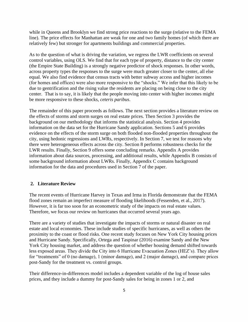
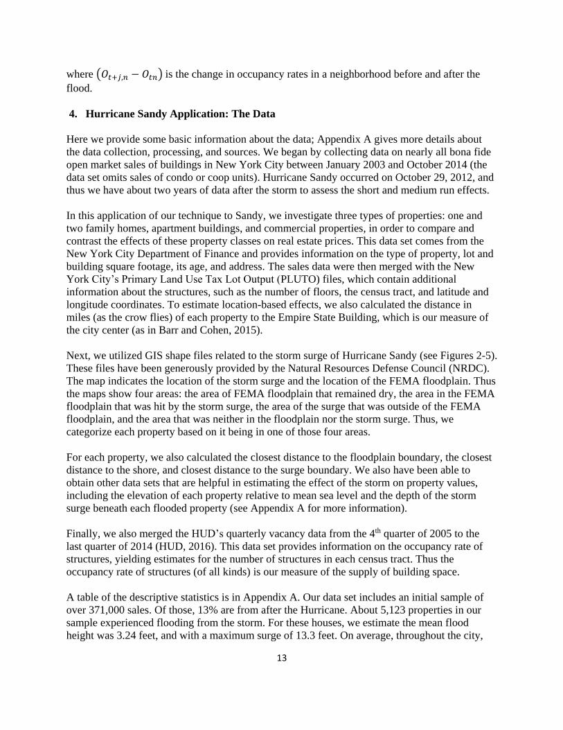
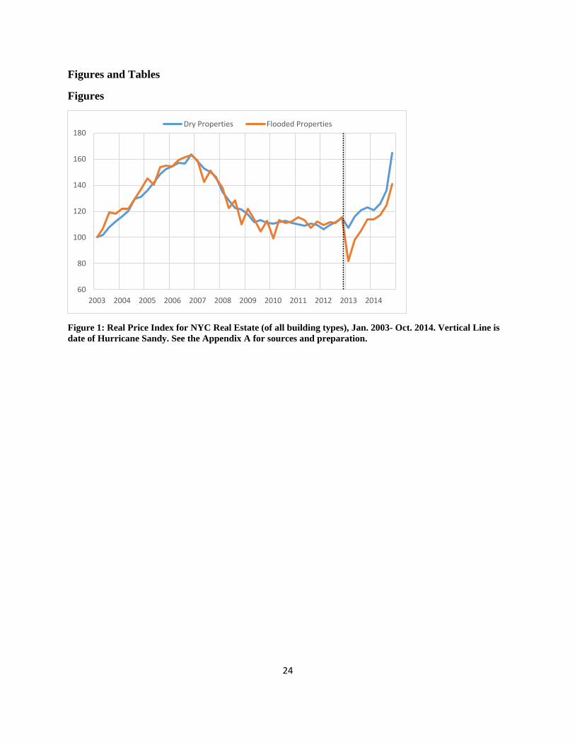
Figure 1 shows two indexes of real estate prices throughout New York City from 2003 and

2014—those properties that remain dry and those that were to be or were flooded by Hurricane

Sandy on October 29, 2012. The indexes come from two hedonic regressions of the log of the

real price of building space per square foot (sales prices divided by the NYC CPI excluding

shelter costs) and a series of building and locational controls (further discussed in this section

and in Appendix A). The results show, as expected, that the two series moved in tandem until the

storm; at that point we observe a sharp reduction the prices in the flooded properties.

Subsequently, the flooded areas experienced a rebound, though have remained below the non-

flooded properties.9

{FIGURE 1 about here—Index of Real Prices}

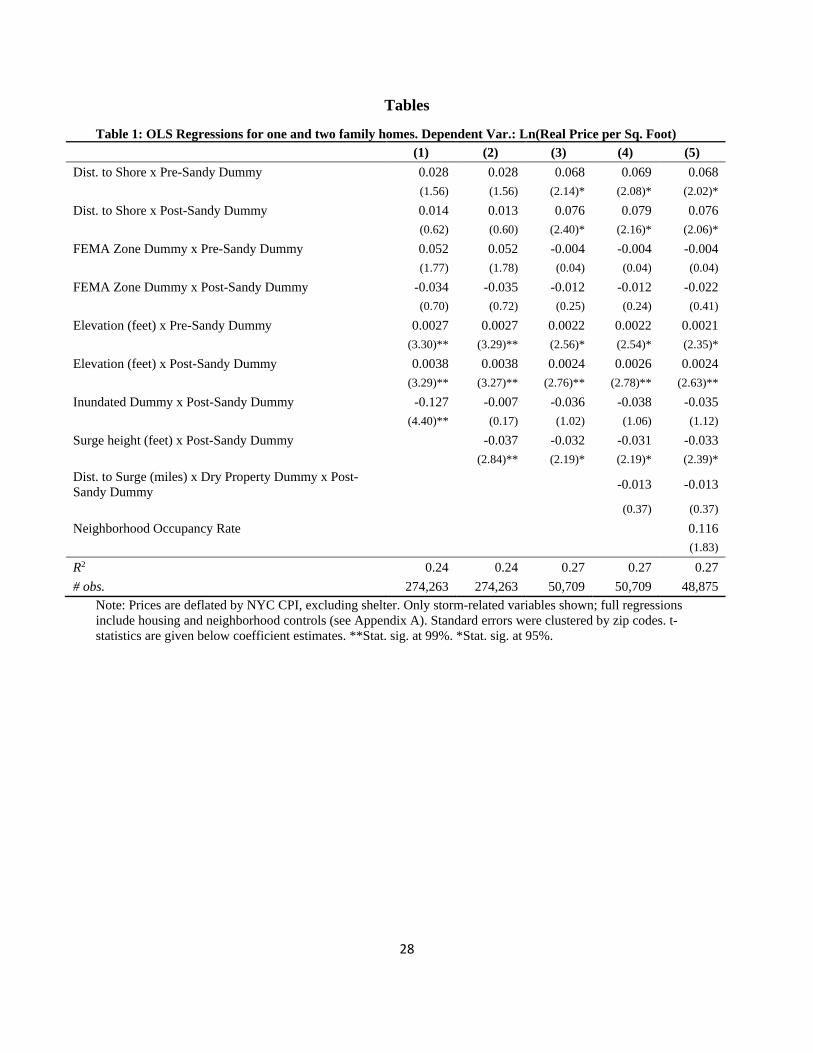
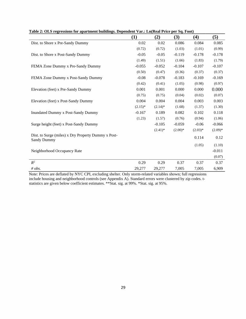
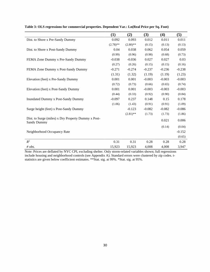
Tables 1 - 3 present the results of hedonic regressions aimed at assessing how the storm affected

real estate prices. Table 1 is for one or two family homes; Table 2 is for apartment buildings, and

Table 3 is for commercial properties. All regressions contain a series of building-level controls

(square footage of property, year built, square footage of lot, # of structures on the property, and

total units, as well as year-quarterly dummies, building type dummies and zip code dummies).

The tables present only the variables that, presumably, are storm-related. The standard errors are

clustered at the zip code level. Each table provides five specifications. In all tables, Equations (1)

and (2) include all the properties in the respective category from January 2003 to October 2014.

Equations (3) - (5) include only properties that are either in the flooded area or within a half-mile

away, and for sales within two years of the storm (i.e., November 2010 to October 2014).

{TABLES 1 - 3 about here—Hedonic Regressions}

The exogenous variables of interest are:

9 It is possible that after the storm, certain types of properties in the flooded areas were more likely to appear on the

market than others (e.g., those less damaged by the storm). To address possible sample selection bias, we first ran a

probit regression, where the dependent variable took on the value of 1 if in the flooded area, 0 otherwise for all

properties (both before and after the storm). Control variables included year-quarter dummies, the property

elevation, the property elevation x a post-Sandy dummy, the distance to the shore, and the distance to the shore x a

post-Sandy dummy. From this regression, we included the Inverse Mills Ratio as an additional control variable.

Note that inclusion of the IMR did not substantially alter the index values, suggesting that sample selection was not

a key problem. Results are available upon request from the authors.

15

1. The distance of the property to shoreline (in miles), interacted with before and after the

storm dummies, respectively;

2. Whether the property was in the FEMA floodplain, interacted with before and after the

storm dummies, respectively;

3. The elevation of the property (in feet), interacted with before and after the storm

dummies, respectively;

4. A dummy variable if the property is flooded by the storm surge times a post-storm

dummy;

5. The height of the storm surge (0 for dry properties), interacted with a post-storm dummy;

6. The distance of the dry properties from the storm surge, interacted with a post-storm

dummy and a dry-property dummy; and

7. The quarterly occupancy rate of structures in their respective census tracts (from 2005Q4

to 2014Q4).

Table 1 shows some interesting results for one and two family houses. Based on the results from

Equation (1), residential properties, on average, lost about 12.7% of their value in the flooded

zone. Equations (2) – (5) show a strong negative relationship between the height of the surge and

the price after the storm. The results show that, on average, a one-foot increase in the storm surge

is associated with about a 3.1 to 3.7% drop in housing prices. The results also suggest higher

elevation became more valuable after the storm. In Equation (5), we do not see evidence that, on

average, dry properties close to the storm experienced any price impacts, but we explore this

issue in more detail below.

The value of being in a FEMA floodplain district is unclear, given that the signs change across

specifications. However, after the storm, all the coefficients for the FEMA floodplain dummy are

negative (though statistically insignificant), suggesting that the property buyers view being in the

FEMA floodplains as a type of an informational disamenity, given that it likely reveals new

information about the likelihood of future storm flooding.

Table 2 contains the same regression specifications but only for apartment buildings. Here we

see that, based on Equation (1), apartment buildings lost about 16.7% of their value, on average,

if they are in the flooded area. Based on Equations (2) to (5), we see that a one-foot increase in

the surge reduced prices between about 6.0 and 10.5%, on average. We also see evidence that the

value of being in the FEMA floodplain became more negative after the storm. There is also

evidence of an elevation premium after the storm—that is, the elevation coefficients increase in

value after Sandy, suggesting that apartment buildings on higher ground become relatively more

valuable.

Finally, Table 3, shows the results for commercial properties. On average, inundated commercial

properties lost about 9.7% of their value (though this is not statistically significant). For flooded

properties, each foot of surge height is associated with 8.2% to 12.3% loss in value. Being in a

FEMA floodplain after the storm yields significant losses for commercial properties, as those

properties experience dramatic price drops. Interestingly, we do not see evidence of an elevation

premium for these properties.

16

In summary, across property types, there is strong evidence that the storm surge created

significant losses in property values, as would be expected. Those properties with greater

flooding lost more value, likely due to the greater damage caused by the storm. For apartment

buildings, we see a strong elevation premium after the storm. Finally, across regressions, being

in the FEMA floodplain after the storm caused properties to lose value. This suggests that the

informational shock about the likelihood of being flooded is larger than the value placed on

having flood insurance.

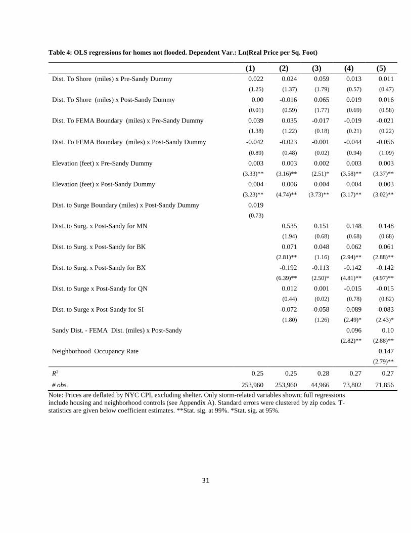
5.1 Effects on Dry Properties

In this section, using ordinary least squares (OLS) regressions, we investigate how the storm

surge might have influenced properties only on the dry side after the storm; that is, properties

that flooded. Tables 4 through 6 present the regression results.

Regarding the FEMA floodplain coefficients, for one and two family homes, there is not much

evidence of an effect. For apartment buildings, the FEMA coefficients are all negative and there

is some evidence that, after the storm, the coefficients become less negative, though, again, they

are not statistically significant. For commercial properties, the effect becomes more negative

after the storm, suggesting that commercial property buyers consider being close the FEMA

boundary as bad news for their properties. For homes and apartments (but not commercial

buildings), there is an elevation premium.

{Table 4 – 6 about here: Hedonic regressions on dry properties}

The coefficient for the distance to the surge boundary is positive (but not significant) across all

three dependent variables. This provides weak evidence that those properties further away from

the flood zone rose in value, on average, as would be expected if there was an informational

shock from the storm.

However, to explore this further, we also interact the borough dummies with the distance from

the surge to see if there are heterogeneous effects across the city. Across dependent variables, for

Brooklyn and Manhattan there are positive effects from being further away from the surge after

the storm. However, there are negative effects for Bronx and Staten Island, which is contrary to

what one might expect.

Importantly, in Equations (4) and (5), across tables, there is a positive effect related to the

distance to surge minus the distance to FEMA zone. This suggests that the informational shock

generated changes in prices for these properties, on average. We explore this finding in more

detail below to see if there is heterogeneity in the response to shocks across the city.

In summary, the key findings of these regressions are that the distance to the surge boundary,

after the storm, for each of the five boroughs, shows positive effects in some cases and negative

in others. We would expect positive in all cases—being further away would be better. Finally,

we find a positive coefficient estimates for Sandy Distance-FEMA Distance, as would be

17

expected. We now turn to the investigating the effects of the storm using LWRs, which allows

us to explore in more detail the heterogeneous effects of the storm surge on the dry properties.

6. Repeat Sales and LWRs for the Dry Properties: LWR Results for New York City

Here we report the results of the LWRs for the repeat sales. When measuring the effects of

Sandy on the dry properties, it is also important to control for other factors that might be

correlated with the shock effect. Because the shock is likely to vary across the city (from north to

south and east to west), latitude and longitude are useful proxies for this spatial variation. Thus,

we included, as spatial controls, the latitude and longitude (in degrees) of each property.

Furthermore, since our data set includes properties with sales either before, during or after the

financial crises and Great Recession, it is also important to include time-related controls, so,

again, we could better isolate the cause of the shock. To this end, we include two time-related

variables: the number of calendar days between the two repeat sales and the year and quarter of

the second sale.10

Descriptive statistics of the LWR coefficients are given in Table 7. OLS regression results the

repeat sales equation for one and two family homes, apartment buildings and commercial

structures, respectively, as well as LWR coefficient estimate histograms, are in Appendix B.

Table 7 shows that, on average, the LWR coefficients for the surge boundary distance minus the

FEMA boundary distance (Surge – FEMA) variable are positive, as would be expected. That is, a

“positive” shock—when the storm did not come as close as the FEMA line—would mean a

relative benefit for those property owners.

The average of the standard deviations of the coefficients are greater than the mean values of the

coefficients, suggesting a relatively large degree of variation for the coefficient estimates. The

ranges of the coefficients show this as well. Furthermore, a test for the non-stationarity of the

coefficients shows that for each of the three dependent variables, we can reject stationarity at

greater than the 99% level of confidence (see Section 8).

In sum, the evidence strongly rejects that OLS estimates accurately measure the relationship

between the storm shock and price changes; rather the LWR estimates are better able to measure

the degree of spatial heterogeneity across the city.

{Table 7 about here—LWR Desc. Stats.}

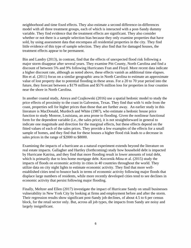
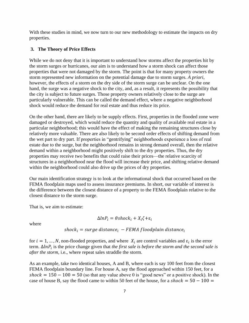
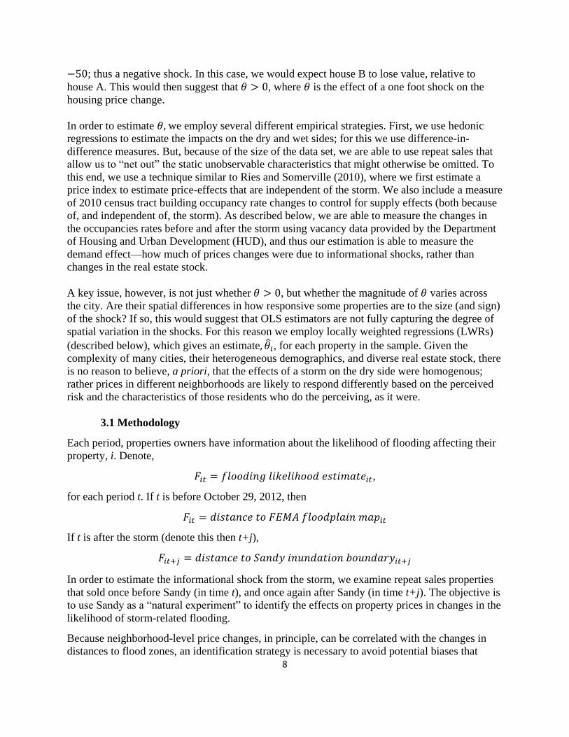
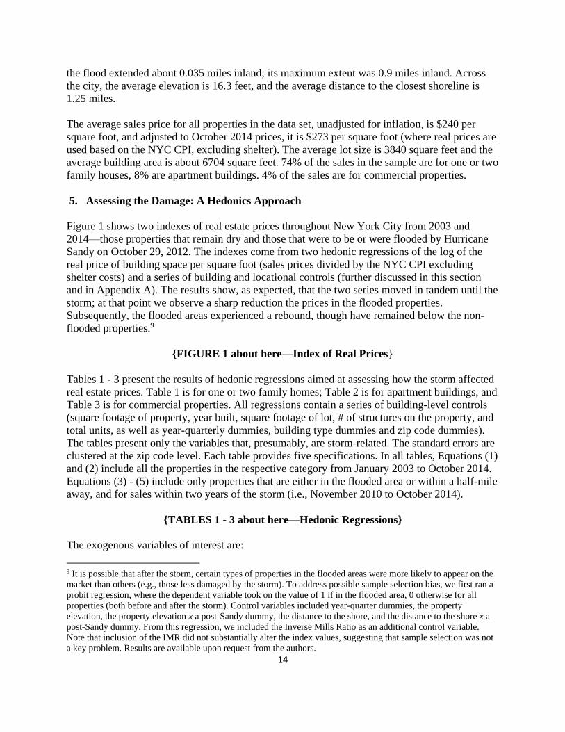
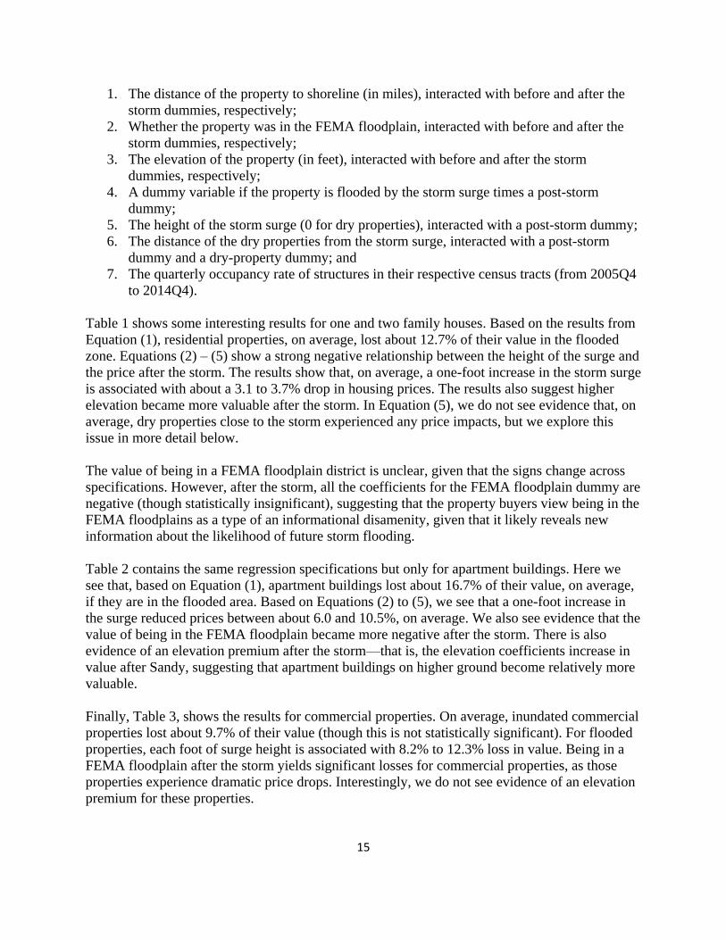
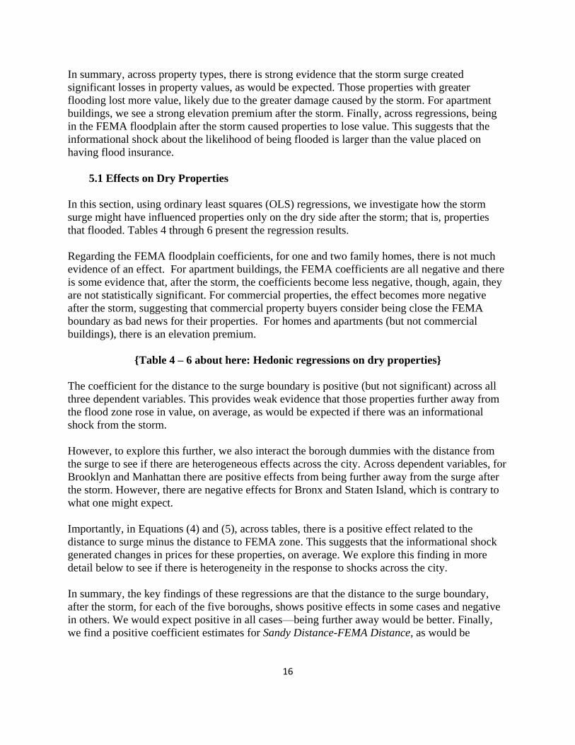
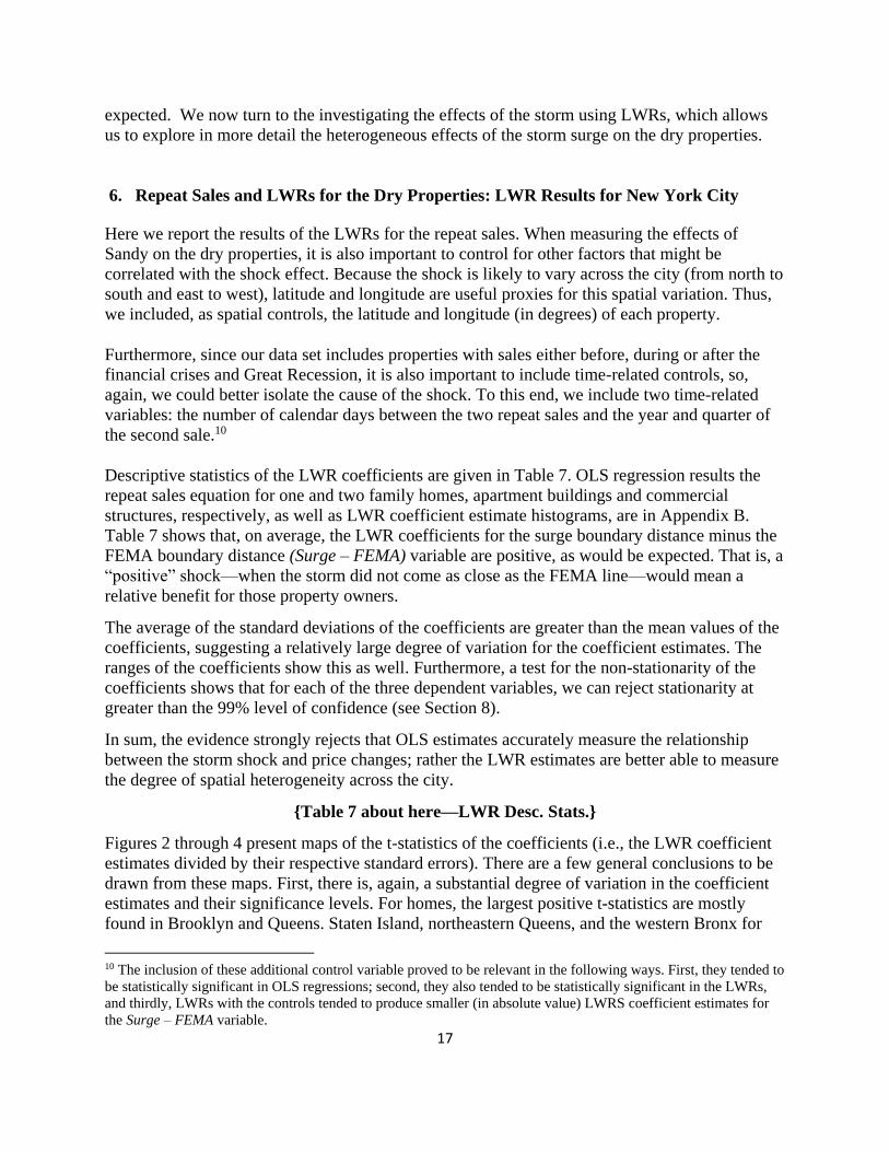
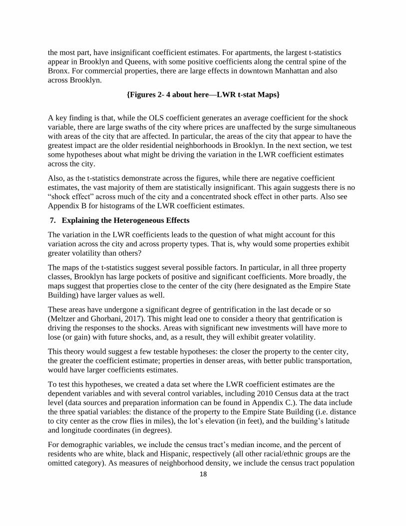
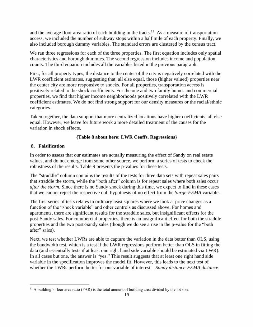
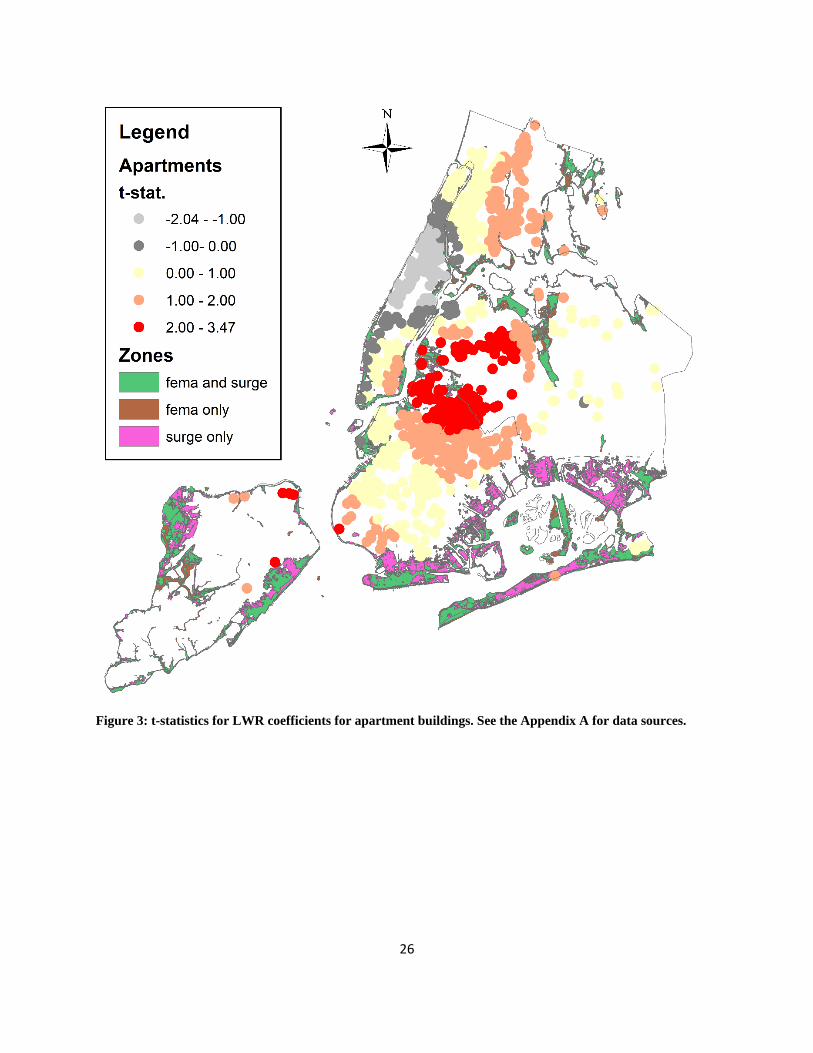
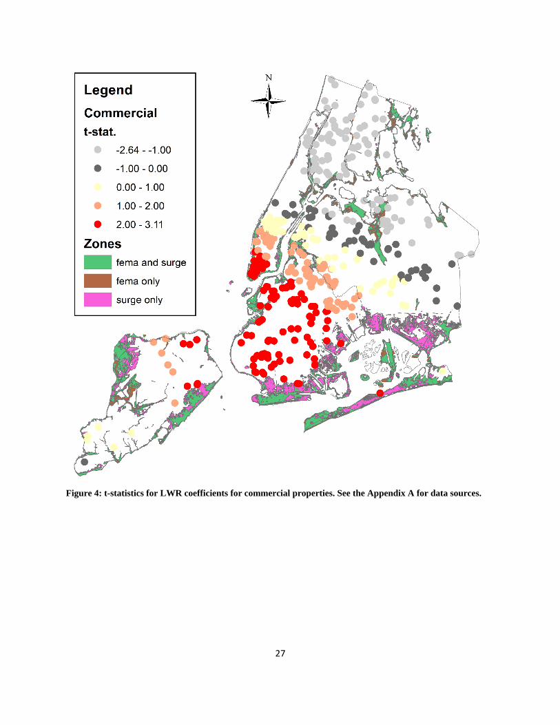
Figures 2 through 4 present maps of the t-statistics of the coefficients (i.e., the LWR coefficient

estimates divided by their respective standard errors). There are a few general conclusions to be

drawn from these maps. First, there is, again, a substantial degree of variation in the coefficient

estimates and their significance levels. For homes, the largest positive t-statistics are mostly

found in Brooklyn and Queens. Staten Island, northeastern Queens, and the western Bronx for

10 The inclusion of these additional control variable proved to be relevant in the following ways. First, they tended to

be statistically significant in OLS regressions; second, they also tended to be statistically significant in the LWRs,

and thirdly, LWRs with the controls tended to produce smaller (in absolute value) LWRS coefficient estimates for

the Surge – FEMA variable.

18

the most part, have insignificant coefficient estimates. For apartments, the largest t-statistics

appear in Brooklyn and Queens, with some positive coefficients along the central spine of the

Bronx. For commercial properties, there are large effects in downtown Manhattan and also

across Brooklyn.

{Figures 2- 4 about here—LWR t-stat Maps}

A key finding is that, while the OLS coefficient generates an average coefficient for the shock

variable, there are large swaths of the city where prices are unaffected by the surge simultaneous

with areas of the city that are affected. In particular, the areas of the city that appear to have the

greatest impact are the older residential neighborhoods in Brooklyn. In the next section, we test

some hypotheses about what might be driving the variation in the LWR coefficient estimates

across the city.

Also, as the t-statistics demonstrate across the figures, while there are negative coefficient

estimates, the vast majority of them are statistically insignificant. This again suggests there is no

“shock effect” across much of the city and a concentrated shock effect in other parts. Also see

Appendix B for histograms of the LWR coefficient estimates.

7. Explaining the Heterogeneous Effects

The variation in the LWR coefficients leads to the question of what might account for this

variation across the city and across property types. That is, why would some properties exhibit

greater volatility than others?

The maps of the t-statistics suggest several possible factors. In particular, in all three property

classes, Brooklyn has large pockets of positive and significant coefficients. More broadly, the

maps suggest that properties close to the center of the city (here designated as the Empire State

Building) have larger values as well.

These areas have undergone a significant degree of gentrification in the last decade or so

(Meltzer and Ghorbani, 2017). This might lead one to consider a theory that gentrification is

driving the responses to the shocks. Areas with significant new investments will have more to

lose (or gain) with future shocks, and, as a result, they will exhibit greater volatility.

This theory would suggest a few testable hypotheses: the closer the property to the center city,

the greater the coefficient estimate; properties in denser areas, with better public transportation,

would have larger coefficients estimates.

To test this hypotheses, we created a data set where the LWR coefficient estimates are the

dependent variables and with several control variables, including 2010 Census data at the tract

level (data sources and preparation information can be found in Appendix C.). The data include

the three spatial variables: the distance of the property to the Empire State Building (i.e. distance

to city center as the crow flies in miles), the lot’s elevation (in feet), and the building’s latitude

and longitude coordinates (in degrees).

For demographic variables, we include the census tract’s median income, and the percent of

residents who are white, black and Hispanic, respectively (all other racial/ethnic groups are the

omitted category). As measures of neighborhood density, we include the census tract population

19

and the average floor area ratio of each building in the tracts.11 As a measure of transportation

access, we included the number of subway stops within a half mile of each property. Finally, we

also included borough dummy variables. The standard errors are clustered by the census tract.

We ran three regressions for each of the three properties. The first equation includes only spatial

characteristics and borough dummies. The second regression includes income and population

counts. The third equation includes all the variables listed in the previous paragraph.

First, for all property types, the distance to the center of the city is negatively correlated with the

LWR coefficient estimates, suggesting that, all else equal, those (higher valued) properties near

the center city are more responsive to shocks. For all properties, transportation access is

positively related to the shock coefficients. For the one and two family homes and commercial

properties, we find that higher income neighborhoods positively correlated with the LWR

coefficient estimates. We do not find strong support for our density measures or the racial/ethnic

categories.

Taken together, the data support that more centralized locations have higher coefficients, all else

equal. However, we leave for future work a more detailed treatment of the causes for the

variation in shock effects.

{Table 8 about here: LWR Ceoffs. Regressions}

8. Falsification

In order to assess that our estimates are actually measuring the effect of Sandy on real estate

values, and do not emerge from some other source, we perform a series of tests to check the

robustness of the results. Table 9 presents the p-values for these tests.

The “straddle” column contains the results of the tests for three data sets with repeat sales pairs

that straddle the storm, while the “both after” column is for repeat sales where both sales occur

after the storm. Since there is no Sandy shock during this time, we expect to find in these cases

that we cannot reject the respective null hypothesis of no effect from the Surge-FEMA variable.

The first series of tests relates to ordinary least squares where we look at price changes as a

function of the “shock variable” and other controls as discussed above. For homes and

apartments, there are significant results for the straddle sales, but insignificant effects for the

post-Sandy sales. For commercial properties, there is an insignificant effect for both the straddle

properties and the two post-Sandy sales (though we do see a rise in the p-value for the “both

after” sales).

Next, we test whether LWRs are able to capture the variation in the data better than OLS, using

the bandwidth test, which is a test if the LWR regressions perform better than OLS in fitting the

data (and essentially tests if at least one right hand side variable should be estimated via LWR).

In all cases but one, the answer is “yes.” This result suggests that at least one right hand side

variable in the specification improves the model fit. However, this leads to the next test of

whether the LWRs perform better for our variable of interest—Sandy distance-FEMA distance.

11 A building’s floor area ratio (FAR) is the total amount of building area divided by the lot size.

20

In this case, we perform tests of nonstationarity of the Sandy-FEMA coefficients. Here the null

hypothesis is that there is no variation in the coefficients and hence LWRs would not be

necessary for that particular variable. We find that we can reject the null in the straddle cases, but

we cannot reject it in the “both after” cases. This finding suggests that there is stationarity in the

“both after” case and that the stationary coefficient is statistically insignificant. In short, the

stationarity test combined with the OLS test suggests that our straddle data is capturing a true

Sandy effect.

{Table 9 falsification about here}

9. Conclusion

This paper develops a methodology to estimate the effects that a major hurricane has on

properties that are not flooded by the storm. In particular, our approach examines how price

changes are affected by the distance to the flood zone relative to the distance of the FEMA

floodplain. Before the storm, the floodplain maps serve to provide information on the likelihood

a flood. After the storm, the distance to the inundation zone provides new information about

future flooding from storm surges. This methodology also uses LWRs to allow for the possibility

that the effects of the surge are heterogonous across a city. Our approach controls for both supply

(i.e., building occupancy) and demand effects, as well as sample selection issues with an inverse

Mills ratio adjustment. We propose using a smooth local price index (i.e., a Fourier repeat sales

price index, as in McMillen and Dombrow, 2001), which controls for neighborhood price

variation independent of the intendent variable of interest.

We demonstrate the use of our methodology with a repeat sales dataset of commercial and

residential properties in New York City that sell once before and once after Hurricane Sandy.

Some neighborhoods, particularly in the outer parts of the city, experience no changes in prices

due to the storm. Other the hand, we see large and statically significant effects in the inner parts

of the city, in particular in neighborhoods in Brooklyn and Queens near Manhattan, which are

suggestive that gentrifying neighborhoods had the largest coefficients. We illustrate these

heterogeneous effects with maps of these properties. We verify the robustness of our estimations

with falsification testing.

Our methodology has the potential to address the real estate impacts of other recent, major

storms, such as Hurricane Harvey and Hurricane Irma. After some time passes and there are

additional data available on properties that sold once before and once after the storm, these

storms’ effects on local real estate markets can be analyzed in detail. Given the prevalence of

major, devastating hurricanes in recent weeks in the U.S., our approach has the potential to help

policy makers estimate the damages from devastating storms, and can also provide information

on the potential benefits that could have been realized if preventative storm surge mitigation had

been undertaken.

21

References

Amemiya, T. (1985). Advanced Econometrics. Cambridge: Harvard University Press. pp. 368–

373.

Anenberg, E., & Laufer, S. Forthcoming. A more timely house price index. Review of

Economics and Statistics.

Atreya, A., & Czajkowski, J. (2016). Graduated Flood Risks and Property Prices in Galveston

County. Real Estate Economics.

Bailey, M. J., Muth, R. F., & Nourse, H. O. (1963). A regression method for real estate price

index construction. Journal of the American Statistical Association, 58(304), 933-942.

Barr, J., & Cohen, J. P. (2014). The floor area ratio gradient: New York City, 1890–

2009. Regional Science and Urban Economics, 48, 110-119.

Bin, O., & Landry, C. E. (2013). Changes in implicit flood risk premiums: Empirical evidence

from the housing market. Journal of Environmental Economics and management, 65(3), 361-

376.

Bin, O., Poulter, B., Dumas, C. F., & Whitehead, J. C. (2011). Measuring the impact of sea‐level

rise on coastal real estate: a hedonic property model approach. Journal of Regional Science,

51(4), 751-767.

CNN (2013). http://www.cnn.com/2013/07/13/world/americas/hurricane-sandy-fast-facts/

Cleveland, W. S., & Devlin, S. J. (1988). Locally weighted regression: an approach to regression

analysis by local fitting. Journal of the American statistical association, 83(403), 596-610.

Deng, Y., McMillen, D.P., & Sing, T.F. (2012). Private residential price indices in Singapore: a

matching approach. Regional Science and Urban Economics. 42(3), 485-494.

ESA (2013). http://www.esa.doc.gov/sites/default/files/sandyfinal101713.pdf . Accessed on

9/16/2017.

FEMA (2017a) https://www.fema.gov/media-library-data/1468504201672-

3c52280b1b1d936e8d23e26f12816017/Flood_Hazard_Mapping_Updates_Overview_Fact_Sheet

.pdf . Accessed on 9/16/2017.

FEMA (2017b). https://www.floodsmart.gov/floodsmart/pages/about/nfip_overview.jsp .

Accessed on 9/16/2017.

Fessenden, F., Gebeloff, R. Walsh, M. W. and Griggs, T. (2017). Water damage from Hurricane

Harvey extended far beyond flood zones.” New York Times, September 1.

https://books.google.com/books?id=0bzGQE14CwEC&pg=PA368

http://www.cnn.com/2013/07/13/world/americas/hurricane-sandy-fast-facts/

http://www.esa.doc.gov/sites/default/files/sandyfinal101713.pdf

https://www.fema.gov/media-library-data/1468504201672-3c52280b1b1d936e8d23e26f12816017/Flood_Hazard_Mapping_Updates_Overview_Fact_Sheet.pdf



https://www.floodsmart.gov/floodsmart/pages/about/nfip_overview.jsp

22

https://www.nytimes.com/interactive/2017/09/01/us/houston-damaged-buildings-in-fema-flood-

zones.html?mcubz=1&_r=1. Accessed on 9/16/2017.

Fotheringham, A. S., & Brunsdon, C. (2002). Geographically Weighted Regression: The

Analysis of Spatially Varying Relationships. Charlton.

Gallagher, J., & Hartley, D. (forthcoming). Household Finance after a Natural Disaster: The

Case of Hurricane Katrina. American Economic Journal: Economic Policy.

Heckman, J.J. (1976). The common structure of statistical models of truncation, sample selection

and limited dependent variables and a simple estimator for such models. Annals of Economic

and Social Measurement. 5(4): 475–492.

Heckman, J.J. (1979). Sample selection as a specification error. Econometrica. 47 (1): 153–161.

HUD (2016). Aggregated USPS Administrative Data on Address Vacancies.

https://www.huduser.gov/portal/usps/home.html Accessed 9/16/2017.

Kocornik-Mina, A., McDermott, T. K., Michaels, G., & Rauch, F. (2015). Flooded cities (No.

11010). CEPR Discussion Papers.

MacDonald, D. N., Murdoch, J. C., & White, H. L. (1987). Uncertain hazards, insurance, and

consumer choice: Evidence from housing markets. Land Economics, 63(4), 361-371.

McMillen, D. P., & Redfearn, C. L. (2010). Estimation and hypothesis testing for nonparametric

hedonic house price functions. Journal of Regional Science, 50(3), 712-733.

McMillen, D. P., & Dombrow, J. (2001). A flexible Fourier approach to repeat sales price

indexes. Real Estate Economics, 29(2), 207.

McMillen, D.P. & McDonald, J.F. (2004). Reaction of house prices to a new rapid transit line:

Chicago's midway line, 1983–1999. Real Estate Economics, 32(3), 463-486.

McMillen, D. P. (2003). Neighborhood house price indexes in Chicago: a Fourier repeat sales

approach. Journal of Economic Geography, 3(1), 57-73.

McWilliams, G. & Marianna, P. (2017). Texas governor says Harvey damage could reach $180

billion. Reuters. Retrieved September 3, 2017.

Metlzer, R., and Ellen, I.G. (2017). Small business vulnerability in the face of natural disasters:

the case of Hurricane Sandy and New York City. Unpublished manuscript.

Meltzer, R., & Ghorbani, P. (2017). Does gentrification increase employment opportunities in

low-Income neighborhoods? Regional Science and Urban Economics.



https://www.huduser.gov/portal/usps/home.html

23

Ortega, F., & Taspinar, S. (2016). Rising sea levels and sinking property values: the effects of

Hurricane Sandy on New York's housing market (No. 10374). Institute for the Study of Labor

(IZA).

Ries, J., & Somerville, T. (2010). School quality and residential property values: evidence from

Vancouver rezoning. The Review of Economics and Statistics, 92(4), 928-944.

Sun-Sentinel. (2017). Tornado warning issued for Broward and Palm Beach Counties, as

thunderstorm spun off by Hurricane Irma”. September 10. Retrieved September 10, 2017.

Wood, Z. (2017). Economic cost of Hurricane Irma 'could reach $300bn'. The Guardian. ISSN

0261-3077. September 10. Retrieved September 13, 2017.

24

Figures and Tables

Figures

Figure 1: Real Price Index for NYC Real Estate (of all building types), Jan. 2003- Oct. 2014. Vertical Line is

date of Hurricane Sandy. See the Appendix A for sources and preparation.

60

80

100

120

140

160

180

2003 2004 2005 2006 2007 2008 2009 2010 2011 2012 2013 2014

Dry Properties Flooded Properties

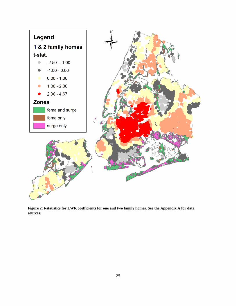
25

Figure 2: t-statistics for LWR coefficients for one and two family homes. See the Appendix A for data

sources.

26

Figure 3: t-statistics for LWR coefficients for apartment buildings. See the Appendix A for data sources.

27

Figure 4: t-statistics for LWR coefficients for commercial properties. See the Appendix A for data sources.

28

Tables

Table 1: OLS Regressions for one and two family homes. Dependent Var.: Ln(Real Price per Sq. Foot)

(1) (2) (3) (4) (5)

Dist. to Shore x Pre-Sandy Dummy 0.028 0.028 0.068 0.069 0.068 (1.56) (1.56) (2.14)* (2.08)* (2.02)*

Dist. to Shore x Post-Sandy Dummy 0.014 0.013 0.076 0.079 0.076 (0.62) (0.60) (2.40)* (2.16)* (2.06)*

FEMA Zone Dummy x Pre-Sandy Dummy 0.052 0.052 -0.004 -0.004 -0.004 (1.77) (1.78) (0.04) (0.04) (0.04)

FEMA Zone Dummy x Post-Sandy Dummy -0.034 -0.035 -0.012 -0.012 -0.022 (0.70) (0.72) (0.25) (0.24) (0.41)

Elevation (feet) x Pre-Sandy Dummy 0.0027 0.0027 0.0022 0.0022 0.0021 (3.30)** (3.29)** (2.56)* (2.54)* (2.35)*

Elevation (feet) x Post-Sandy Dummy 0.0038 0.0038 0.0024 0.0026 0.0024 (3.29)** (3.27)** (2.76)** (2.78)** (2.63)**

Inundated Dummy x Post-Sandy Dummy -0.127 -0.007 -0.036 -0.038 -0.035 (4.40)** (0.17) (1.02) (1.06) (1.12)

Surge height (feet) x Post-Sandy Dummy -0.037 -0.032 -0.031 -0.033 (2.84)** (2.19)* (2.19)* (2.39)*

Dist. to Surge (miles) x Dry Property Dummy x Post-

Sandy Dummy -0.013 -0.013

(0.37) (0.37)

Neighborhood Occupancy Rate 0.116

(1.83)

R2 0.24 0.24 0.27 0.27 0.27

# obs. 274,263 274,263 50,709 50,709 48,875

Note: Prices are deflated by NYC CPI, excluding shelter. Only storm-related variables shown; full regressions

include housing and neighborhood controls (see Appendix A). Standard errors were clustered by zip codes. t-

statistics are given below coefficient estimates. **Stat. sig. at 99%. *Stat. sig. at 95%.

29

Table 2: OLS regressions for apartment buildings. Dependent Var.: Ln(Real Price per Sq. Foot)

(1) (2) (3) (4) (5)

Dist. to Shore x Pre-Sandy Dummy 0.02 0.02 0.086 0.084 0.085 (0.72) (0.72) (1.03) (1.01) (0.99)

Dist. to Shore x Post-Sandy Dummy -0.05 -0.05 -0.119 -0.178 -0.178 (1.49) (1.51) (1.66) (1.83) (1.79)

FEMA Zone Dummy x Pre-Sandy Dummy -0.055 -0.052 -0.104 -0.107 -0.107 (0.50) (0.47) (0.36) (0.37) (0.37)


Elevation (feet) x Pre-Sandy Dummy 0.001 0.001 0.000 0.000 0.000 (0.75) (0.75) (0.04) (0.02) (0.07)

Elevation (feet) x Post-Sandy Dummy 0.004 0.004 0.004 0.003 0.003 (2.15)* (2.14)* (1.68) (1.37) (1.30)

Inundated Dummy x Post-Sandy Dummy -0.167 0.189 0.082 0.102 0.118 (1.23) (1.57) (0.76) (0.94) (1.06)

Surge height (feet) x Post-Sandy Dummy -0.105 -0.059 -0.06 -0.066 (2.41)* (2.00)* (2.03)* (2.09)*


Sandy Dummy 0.114 0.12

(1.05) (1.10)

Neighborhood Occupancy Rate -0.011

(0.07)

R2 0.29 0.29 0.37 0.37 0.37

# obs. 29,277 29,277 7,005 7,005 6,909




30

Table 3: OLS regressions for commercial properties. Dependent Var.: Ln(Real Price per Sq. Foot)

(1) (2) (3) (4) (5)

Dist. to Shore x Pre-Sandy Dummy 0.092 0.093 0.012 0.011 0.011 (2.78)** (2.80)** (0.15) (0.13) (0.13)

Dist. to Shore x Post-Sandy Dummy 0.04 0.038 0.062 0.054 0.059 (0.99) (0.96) (0.98) (0.68) (0.73)

FEMA Zone Dummy x Pre-Sandy Dummy -0.038 -0.036 0.027 0.027 0.03 (0.27) (0.26) (0.15) (0.15) (0.16)


Elevation (feet) x Pre-Sandy Dummy 0.001 0.001 -0.003 -0.003 -0.003 (0.72) (0.73) (0.66) (0.65) (0.74)

Elevation (feet) x Post-Sandy Dummy 0.001 0.001 -0.003 -0.003 -0.003 (0.44) (0.33) (0.92) (0.90) (0.84)

Inundated Dummy x Post-Sandy Dummy -0.097 0.237 0.148 0.15 0.178 (1.06) (1.43) (0.91) (0.91) (1.09)

Surge height (feet) x Post-Sandy Dummy -0.123 -0.082 -0.082 -0.086 (2.81)** (1.73) (1.73) (1.86)


Sandy Dummy 0.021 0.006

(0.14) (0.04)


(0.65)

R2 0.31 0.31 0.28 0.28 0.28

# obs. 15,923 15,923 4,008 4,008 3,947




31

Table 4: OLS regressions for homes not flooded. Dependent Var.: Ln(Real Price per Sq. Foot)

(1) (2) (3) (4) (5)

Dist. To Shore (miles) x Pre-Sandy Dummy 0.022 0.024 0.059 0.013 0.011

(1.25) (1.37) (1.79) (0.57) (0.47)

Dist. To Shore (miles) x Post-Sandy Dummy 0.00 -0.016 0.065 0.019 0.016

(0.01) (0.59) (1.77) (0.69) (0.58)

Dist. To FEMA Boundary (miles) x Pre-Sandy Dummy 0.039 0.035 -0.017 -0.019 -0.021

(1.38) (1.22) (0.18) (0.21) (0.22)

Dist. To FEMA Boundary (miles) x Post-Sandy Dummy -0.042 -0.023 -0.001 -0.044 -0.056

(0.89) (0.48) (0.02) (0.94) (1.09)

Elevation (feet) x Pre-Sandy Dummy 0.003 0.003 0.002 0.003 0.003

(3.33)** (3.16)** (2.51)* (3.58)** (3.37)**

Elevation (feet) x Post-Sandy Dummy 0.004 0.006 0.004 0.004 0.003

(3.23)** (4.74)** (3.73)** (3.17)** (3.02)**

Dist. to Surge Boundary (miles) x Post-Sandy Dummy 0.019 (0.73)

Dist. to Surg. x Post-Sandy for MN 0.535 0.151 0.148 0.148

(1.94) (0.68) (0.68) (0.68)

Dist. to Surg. x Post-Sandy for BK 0.071 0.048 0.062 0.061

(2.81)** (1.16) (2.94)** (2.88)**

Dist. to Surg. x Post-Sandy for BX -0.192 -0.113 -0.142 -0.142

(6.39)** (2.50)* (4.81)** (4.97)**

Dist. to Surge x Post-Sandy for QN 0.012 0.001 -0.015 -0.015

(0.44) (0.02) (0.78) (0.82)

Dist. to Surge x Post-Sandy for SI -0.072 -0.058 -0.089 -0.083

(1.80) (1.26) (2.49)* (2.43)*

Sandy Dist. - FEMA Dist. (miles) x Post-Sandy 0.096 0.10

(2.82)** (2.88)**


(2.79)**

R2 0.25 0.25 0.28 0.27 0.27

# obs. 253,960 253,960 44,966 73,802 71,856


include housing and neighborhood controls (see Appendix A). Standard errors were clustered by zip codes. T-


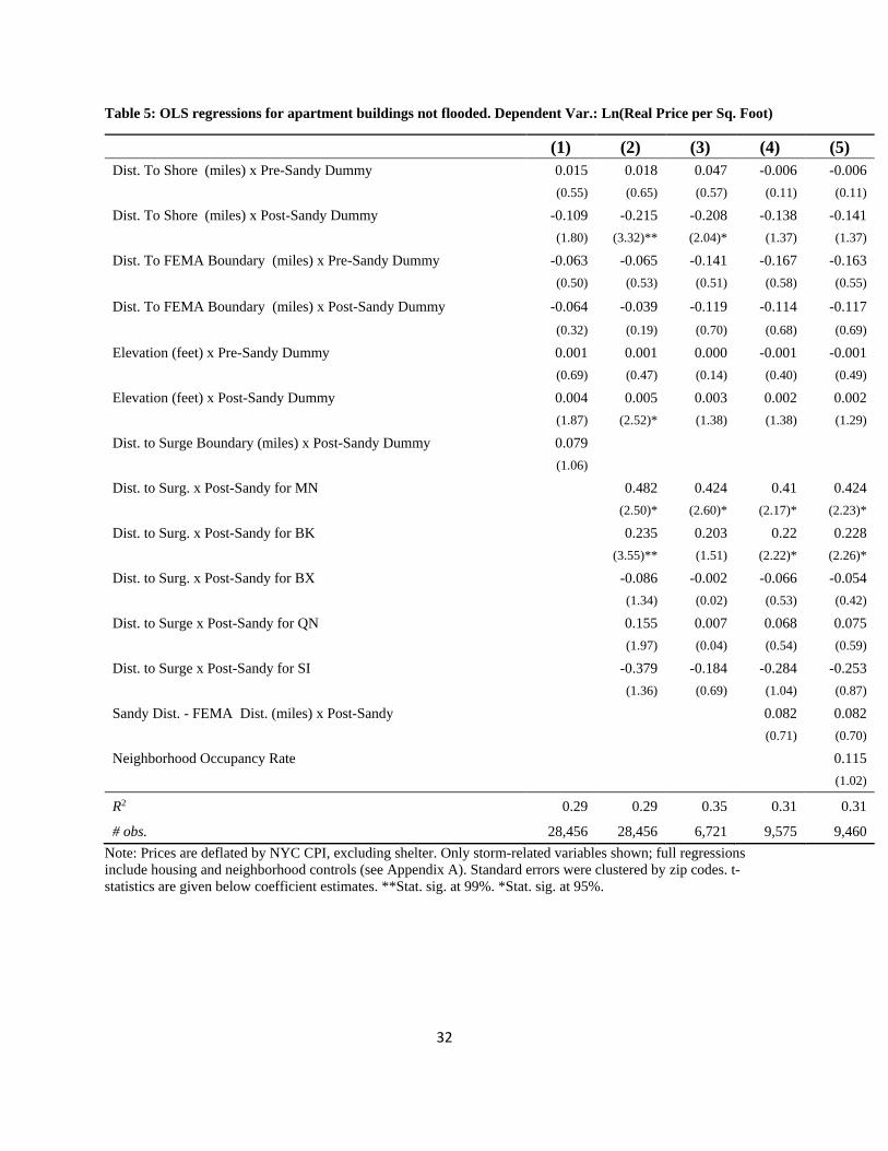
32

Table 5: OLS regressions for apartment buildings not flooded. Dependent Var.: Ln(Real Price per Sq. Foot)

(1) (2) (3) (4) (5)

Dist. To Shore (miles) x Pre-Sandy Dummy 0.015 0.018 0.047 -0.006 -0.006

(0.55) (0.65) (0.57) (0.11) (0.11)

Dist. To Shore (miles) x Post-Sandy Dummy -0.109 -0.215 -0.208 -0.138 -0.141

(1.80) (3.32)** (2.04)* (1.37) (1.37)

Dist. To FEMA Boundary (miles) x Pre-Sandy Dummy -0.063 -0.065 -0.141 -0.167 -0.163

(0.50) (0.53) (0.51) (0.58) (0.55)


(0.32) (0.19) (0.70) (0.68) (0.69)

Elevation (feet) x Pre-Sandy Dummy 0.001 0.001 0.000 -0.001 -0.001

(0.69) (0.47) (0.14) (0.40) (0.49)

Elevation (feet) x Post-Sandy Dummy 0.004 0.005 0.003 0.002 0.002

(1.87) (2.52)* (1.38) (1.38) (1.29)

Dist. to Surge Boundary (miles) x Post-Sandy Dummy 0.079

(1.06)


(2.50)* (2.60)* (2.17)* (2.23)*


(3.55)** (1.51) (2.22)* (2.26)*


(1.34) (0.02) (0.53) (0.42)

Dist. to Surge x Post-Sandy for QN 0.155 0.007 0.068 0.075

(1.97) (0.04) (0.54) (0.59)


(1.36) (0.69) (1.04) (0.87)


(0.71) (0.70)


(1.02)

R2 0.29 0.29 0.35 0.31 0.31

# obs. 28,456 28,456 6,721 9,575 9,460




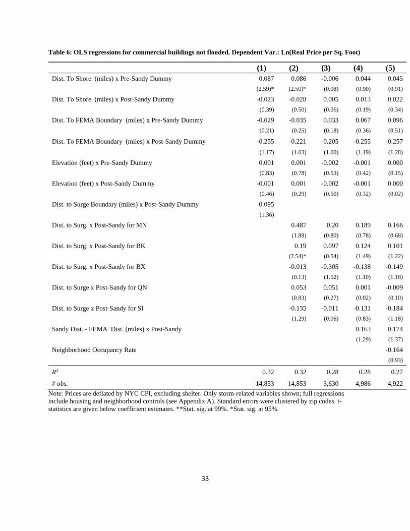
33

Table 6: OLS regressions for commercial buildings not flooded. Dependent Var.: Ln(Real Price per Sq. Foot)

(1) (2) (3) (4) (5)

Dist. To Shore (miles) x Pre-Sandy Dummy 0.087 0.086 -0.006 0.044 0.045

(2.59)* (2.50)* (0.08) (0.90) (0.91)

Dist. To Shore (miles) x Post-Sandy Dummy -0.023 -0.028 0.005 0.013 0.022

(0.39) (0.50) (0.06) (0.19) (0.34)

Dist. To FEMA Boundary (miles) x Pre-Sandy Dummy -0.029 -0.035 0.033 0.067 0.096

(0.21) (0.25) (0.18) (0.36) (0.51)


(1.17) (1.03) (1.00) (1.19) (1.28)

Elevation (feet) x Pre-Sandy Dummy 0.001 0.001 -0.002 -0.001 0.000

(0.83) (0.78) (0.53) (0.42) (0.15)

Elevation (feet) x Post-Sandy Dummy -0.001 0.001 -0.002 -0.001 0.000

(0.46) (0.29) (0.50) (0.32) (0.02)

Dist. to Surge Boundary (miles) x Post-Sandy Dummy 0.095

(1.36)


(1.88) (0.80) (0.78) (0.68)


(2.54)* (0.54) (1.49) (1.22)


(0.13) (1.52) (1.10) (1.18)

Dist. to Surge x Post-Sandy for QN 0.053 0.051 0.001 -0.009

(0.83) (0.27) (0.02) (0.10)


(1.29) (0.06) (0.83) (1.18)


(1.29) (1.37)


(0.93)

R2 0.32 0.32 0.28 0.28 0.27

# obs. 14,853 14,853 3,630 4,986 4,922




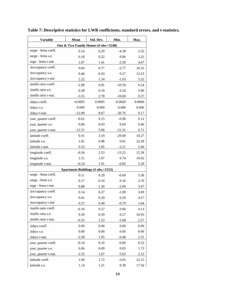
34

Table 7: Descriptive statistics for LWR coefficients, standard errors, and t-statistics.

Variable Mean Std. Dev. Min. Max.

One & Two Family Homes (# obs.=5248)

surge - fema coeff. 0.14 0.29 -4.39 3.35

surge - fema s.e. 0.18 0.22 0.06 3.25

suge - fema t-stat 1.07 1.41 -2.50 4.67

∆occupancy coeff. 0.83 0.77 -2.77 16.35

∆occupancy s.e. 0.46 0.43 0.27 12.23

∆occupancy t-stat 2.22 1.34 -1.03 5.52

∆mills ratio coeff. -1.89 0.81 -10.59 0.24

∆mills ratio s.e. 0.38 0.19 0.24 3.96

∆mills ratio t-stat. -5.55 2.78 -10.69 0.57

∆days coeff. -0.0005 0.0005 -0.0020 0.0000

∆days s.e. 0.000 0.000 0.000 0.000

∆days t-stat. -12.89 8.67 -30.76 0.17

year_quarter coeff. -0.61 0.15 -0.96 0.12

year_quarter s.e. 0.06 0.03 0.04 0.46

year_quarter t-stat. -12.51 5.06 -21.31 0.71

latitude coeff. 0.41 3.19 -29.69 10.27

latitude s.e. 1.81 0.98 0.81 22.30

latitude t-stat. 0.33 1.85 -3.21 5.66

longitude coeff. -0.56 2.53 -13.22 12.38

longitude s.e. 1.51 1.07 0.74 16.02

longitude t-stat. -0.24 1.91 -6.82 5.29

Apartment Buildings (# obs.=1553)

surge - fema coeff. 0.11 0.29 -0.69 5.28

surge - fema s.e. 0.17 0.19 0.10 3.70

suge - fema t-stat 0.88 1.30 -2.04 3.47

∆occupancy coeff. 0.14 0.27 -1.89 3.09

∆occupancy s.e. 0.41 0.29 0.29 4.57

∆occupancy t-stat 0.37 0.49 -0.79 1.64

∆mills ratio coeff. -0.16 0.57 -3.60 4.13

∆mills ratio s.e. 0.39 0.59 0.27 10.95

∆mills ratio t-stat. -0.55 1.53 -2.68 2.57

∆days coeff. 0.00 0.00 0.00 0.00

∆days s.e. 0.00 0.00 0.00 0.00

∆days t-stat. -3.58 1.95 -6.48 2.31


year_quarter s.e. 0.06 0.09 0.05 1.73


latitude coeff. 1.60 1.72 -3.05 22.15

latitude s.e. 1.14 1.21 0.39 17.56

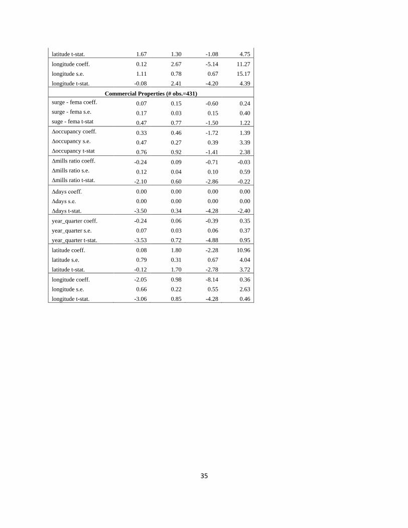
35

latitude t-stat. 1.67 1.30 -1.08 4.75

longitude coeff. 0.12 2.67 -5.14 11.27

longitude s.e. 1.11 0.78 0.67 15.17

longitude t-stat. -0.08 2.41 -4.20 4.39

Commercial Properties (# obs.=431)

surge - fema coeff. 0.07 0.15 -0.60 0.24

surge - fema s.e. 0.17 0.03 0.15 0.40

suge - fema t-stat 0.47 0.77 -1.50 1.22

∆occupancy coeff. 0.33 0.46 -1.72 1.39

∆occupancy s.e. 0.47 0.27 0.39 3.39

∆occupancy t-stat 0.76 0.92 -1.41 2.38

∆mills ratio coeff. -0.24 0.09 -0.71 -0.03

∆mills ratio s.e. 0.12 0.04 0.10 0.59

∆mills ratio t-stat. -2.10 0.60 -2.86 -0.22

∆days coeff. 0.00 0.00 0.00 0.00

∆days s.e. 0.00 0.00 0.00 0.00

∆days t-stat. -3.50 0.34 -4.28 -2.40


year_quarter s.e. 0.07 0.03 0.06 0.37


latitude coeff. 0.08 1.80 -2.28 10.96

latitude s.e. 0.79 0.31 0.67 4.04

latitude t-stat. -0.12 1.70 -2.78 3.72

longitude coeff. -2.05 0.98 -8.14 0.36

longitude s.e. 0.66 0.22 0.55 2.63

longitude t-stat. -3.06 0.85 -4.28 0.46

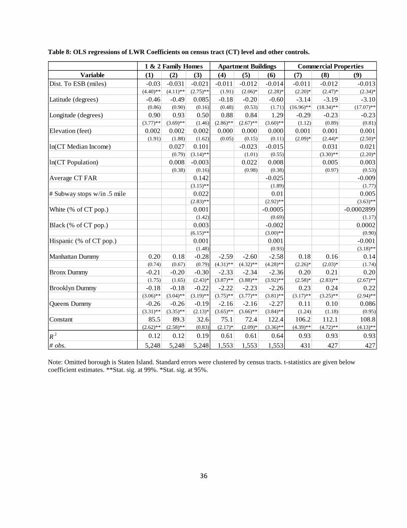
36

Table 8: OLS regressions of LWR Coefficients on census tract (CT) level and other controls.

Variable (1) (2) (3) (4) (5) (6) (7) (8) (9)

Dist. To ESB (miles) -0.03 -0.031 -0.021 -0.011 -0.012 -0.014 -0.011 -0.012 -0.013(4.40)** (4.11)** (2.75)** (1.91) (2.06)* (2.28)* (2.20)* (2.47)* (2.34)*

Latitude (degrees) -0.46 -0.49 0.085 -0.18 -0.20 -0.60 -3.14 -3.19 -3.10(0.86) (0.90) (0.16) (0.48) (0.53) (1.71) (16.96)** (18.34)** (17.07)**

Longitude (degrees) 0.90 0.93 0.50 0.88 0.84 1.29 -0.29 -0.23 -0.23(3.77)** (3.69)** (1.46) (2.86)** (2.67)** (3.60)** (1.12) (0.89) (0.81)

Elevation (feet) 0.002 0.002 0.002 0.000 0.000 0.000 0.001 0.001 0.001(1.91) (1.88) (1.62) (0.05) (0.15) (0.11) (2.09)* (2.44)* (2.50)*

ln(CT Median Income) 0.027 0.101 -0.023 -0.015 0.031 0.021(0.79) (3.14)** (1.01) (0.55) (3.30)** (2.20)*

ln(CT Population) 0.008 -0.003 0.022 0.008 0.005 0.003(0.38) (0.16) (0.98) (0.38) (0.97) (0.53)

Average CT FAR 0.142 -0.025 -0.009(3.15)** (1.89) (1.77)

# Subway stops w/in .5 mile 0.022 0.01 0.005(2.83)** (2.92)** (3.63)**

White (% of CT pop.) 0.001 -0.0005 -0.0002899(1.42) (0.69) (1.17)

Black (% of CT pop.) 0.003 -0.002 0.0002(6.15)** (3.00)** (0.90)

Hispanic (% of CT pop.) 0.001 0.001 -0.001(1.48) (0.93) (3.18)**

Manhattan Dummy 0.20 0.18 -0.28 -2.59 -2.60 -2.58 0.18 0.16 0.14(0.74) (0.67) (0.79) (4.31)** (4.32)** (4.28)** (2.26)* (2.03)* (1.74)

Bronx Dummy -0.21 -0.20 -0.30 -2.33 -2.34 -2.36 0.20 0.21 0.20(1.75) (1.65) (2.43)* (3.87)** (3.88)** (3.92)** (2.58)* (2.83)** (2.67)**

Brooklyn Dummy -0.18 -0.18 -0.22 -2.22 -2.23 -2.26 0.23 0.24 0.22(3.06)** (3.04)** (3.19)** (3.75)** (3.77)** (3.81)** (3.17)** (3.25)** (2.94)**

Queens Dummy -0.26 -0.26 -0.19 -2.16 -2.16 -2.27 0.11 0.10 0.086(3.31)** (3.35)** (2.13)* (3.65)** (3.66)** (3.84)** (1.24) (1.18) (0.95)

Constant 85.5 89.3 32.6 75.1 72.4 122.4 106.2 112.1 108.8(2.62)** (2.58)** (0.83) (2.17)* (2.09)* (3.36)** (4.39)** (4.72)** (4.13)**

R2 0.12 0.12 0.19 0.61 0.61 0.64 0.93 0.93 0.93

# obs. 5,248 5,248 5,248 1,553 1,553 1,553 431 427 427

1 & 2 Family Homes Apartment Buildings Commercial Properties

Note: Omitted borough is Staten Island. Standard errors were clustered by census tracts. t-statistics are given below

coefficient estimates. **Stat. sig. at 99%. *Stat. sig. at 95%.

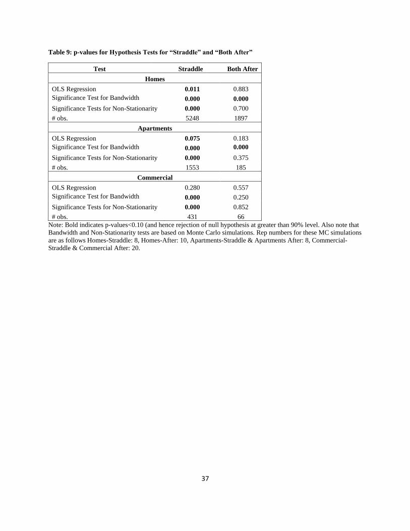
37

Table 9: p-values for Hypothesis Tests for “Straddle” and “Both After”

Test Straddle Both After

Homes

OLS Regression 0.011 0.883

Significance Test for Bandwidth 0.000 0.000

Significance Tests for Non-Stationarity 0.000 0.700

# obs. 5248 1897

Apartments




# obs. 1553 185

Commercial




# obs. 431 66

Note: Bold indicates p-values<0.10 (and hence rejection of null hypothesis at greater than 90% level. Also note that

Bandwidth and Non-Stationarity tests are based on Monte Carlo simulations. Rep numbers for these MC simulations

are as follows Homes-Straddle: 8, Homes-After: 10, Apartments-Straddle & Apartments After: 8, Commercial-

Straddle & Commercial After: 20.

38

Appendix

Appendix A: Data and Regression Results.

A.1. The Data Set

The full processed data set that we used for our analysis has 326,122 real estate sales between January 2003 and

October 2014 throughout the entire city of New York. The data set has nearly every type of building, including one

and two family homes, offices, factories, apartment buildings, etc. In short, it has both residential and commercial

properties. The source of the real estate transactions is the New York City Department of Finance (DoF) website,

http://www1.nyc.gov/site/finance/taxes/property-annualized-sales-update.page. Data include sales price, date of sale,

building address, some details about the property, including the square foot of building, the square foot of lot, year

constructed, and the type of property. Note that this data is only for building sales and excludes condo or coop unit

sales.

Table A.1 lists the different property types and categories that were used in this paper. Building types information

can be found in the NYC PLUTO data dictionary, https://www1.nyc.gov/assets/planning/download/pdf/data-

maps/open-data/pluto_datadictionary.pdf?r=16v2.

{Table A.1 here—Building Types and Frequencies}

The data downloaded from the DoF includes all transfer of title and does not distinguish open market transactions

from the rest. As a result, we were required to process the data and make some assumptions in order to create a data

set that seemed to include only open market sales. First, we deleted observations that had no data for lot size,

building size, year of construction or were sold for less than $100. Then we generated the price per square foot for

each property. In the hedonic regressions (Tables 1-6) we excluded from the regressions those properties that had

price per square foot in the bottom one and top one percentiles, respectively, to avoid the influence of outliers.

Each lot in New York City is assigned a unique borough, block and lot (BBL) number. Using the BBL we then

merged the sales data with the 2014 Primary Land Use Tax Lot Output (PLUTO) file, which details property

characteristics for every BBL in the city, some of which overlap with the salse data and some do not. The PLUTO

file includes additional information, such as the property latitude and longitude, and the number of floors of the

building. The PLUTO file is available at https://www1.nyc.gov/site/planning/data-maps/open-data/dwn-pluto-

mappluto.page. For the hedonic regressions, we adjusted the sales price by the NYC CPI without shelter

(CUURA101SASL2RS), with the first quarter of 2014 as the base period.

Sandy flooding maps and FEMA insurance flood maps were generously provided by the National Resources

Defense Council (NRDC). They provided us with GIS shape files that indicated the locations in the city of the surge

flood, and the locations of FEMA floodplain. We used the same files as shown in Figure 1 of their report on Sanday,

at https://www.nrdc.org/sites/default/files/hurricane-sandy-coastal-flooding-report.pdf.

Using this information, we then created our Sandy-related variables, which include the distance to the flood zone

boundary for all properties, the distance to the shoreline, and the distance to the FEMA floodplain boundary. For

flooded properties, we ascertained whether the building was in the FEMA floodplain map that was in effect in 2012.

We also used the NRDC shape file to ascertain the distance of each property to the closest shoreline. In addition, we

obtained the elevation of each property from the New York City Digital Evolution model, at

http://opengeometadata.stanford.edu/metadata/org.opengeoportal/Columbia:Columbia.usgs_nyc1999_1m/fgdc.html.

The depth of the surge across the city was ascertained from the file “NYC_Feb14Final1mSurgeDataClipped.zip,”

available at https://www.arcgis.com/home/item.html?id=307dd522499d4a44a33d7296a5da5ea0.

Table A.2 gives the descriptive statistics for the data set.

{Table A.2 about here Desc. Stats}

http://www1.nyc.gov/site/finance/taxes/property-annualized-sales-update.page

https://www1.nyc.gov/assets/planning/download/pdf/data-maps/open-data/pluto_datadictionary.pdf?r=16v2

https://www1.nyc.gov/assets/planning/download/pdf/data-maps/open-data/pluto_datadictionary.pdf?r=16v2

https://www1.nyc.gov/site/planning/data-maps/open-data/dwn-pluto-mappluto.page

https://www1.nyc.gov/site/planning/data-maps/open-data/dwn-pluto-mappluto.page

https://www.nrdc.org/sites/default/files/hurricane-sandy-coastal-flooding-report.pdf

http://opengeometadata.stanford.edu/metadata/org.opengeoportal/Columbia:Columbia.usgs_nyc1999_1m/fgdc.html

https://www.arcgis.com/home/item.html?id=307dd522499d4a44a33d7296a5da5ea0

39

Table A.3 gives regression results for one and two family homes, apartment buildings and commercial properties

respectively. For the sake of brevity, we only include one specification for each property type, which is also

Equation (5) in Tables 2-4. However, here, we do not restrict the sample period or distance to the shore in Table

A.3. Other specifications are available upon request.

Also note that the regressions for the price index (Figure 1) regressed the log of the real price per square foot on the

following controls: distance to the Empire State Building, number of floors, number of units, number of buildings on

property, ln(Land Area), ln(Building Area), year built, year-quarterly dummies, building class dummies and zip

code dummies. Standard errors were clustered at the zip code level. We ran two regression one for only the dry

properties and the other for the properties that experienced flooding. In the second equation, we also included an

inverse Mill ratio that was calculated from a probit that estimated the probability that a property would be in the

surge area. That is the dependent variable was equal to 1 if it was flooded or in the flood zone (prior to flooding), 0

otherwise. Controls included year-quarterly dummies, building elevation, building elevation x post-Sandy dummy,

the distance to the shoreline, and the distance to shoreline x post-Sandy dummy. Results available upon request.

For the index, the base year was 2003Q1. We created the index by taking the exponent of the coefficients for the

year-quarterly dummy variables and multiplying them by100, i.e. 𝑖𝑛𝑑𝑒𝑥 𝑣𝑎𝑙𝑢𝑒𝑡 = 100 ∗ 𝑒𝑥𝑝(�̂�𝑡), where �̂�𝑡 , is the

coefficient estimate for year-quarter t. Note �̂�2002𝑄1 = 0 because it was omitted from the regression. Thus

2003Q1=100.

{A.3. Regression Tables for Data Set}

A.2. Repeat Sales

The master data set described above has a significant number of repeat sales. In particular, for each property type

(one and two family homes, apartment buildings, and commercial properties), we created new data sets that

contained each of these repeat sales. We excluded any property if we observed a change in square footage,

construction year, building class type on the assumption that the nature of the property changed over time.

From these remaining properties, we generated sales data sets where for each properties with at least two sales, we

included those properties that had at least one sale before the storm and one sale after (i.e., has repeat sales that

straddled the storm). These straddle data sets needed to be further processed. First, to simplify the analysis we

decided to include only pairs of repeat sales. The included pairs where cases where the first sale occurred closest to

before the storm date and the second sale occurred closest to the storm after the date. To mitigate against included

property “flips” (i.e., those repeat sales that bought and sold for speculation and may have included renovations), we

excluded pairs if the second sale took place within 30 days of the firsr. Lastly, we excluded those sales where the log

of the price changes were either in the top or bottom one percentiles, respectively, within each property category.

Table A.4. Presents the descriptive statistics for the difference of the key variables included in the locally weighted

regressions.

{Table. A.4. about here: Desc. Stats for Straddle Repeats}

A.3. Probits for Inverse Mills Ratio for Repeat Sales

As described in Section 3, we first ran probit regressions (for the dry properties only) to estimate the probability of

repeat sales occurring. The dependent variable takes on the value of 1 if a second or third sales takes place for a

particular property in the data set, 0 otherwise. Control variables included the census tract occupancy rate, the

distance to the Empire State Building, the number of floors, ln(Land Area), ln(Building Area), year built, distance to

shore x pre-Sandy dummy, distance to shore x post-Sandy dummy, FEMA dummy x pre-Sandy dummy, FEMA

dummy x post-Sandy dummy, elevation x pre-Sandy dummy, elevation x post-Sandy dummy, distance to the surge x

outside surge dummy x post-Sandy dummy, year-quarterly dummies and building class dummies. Table A.5 gives

the results.

40

{Table A.5 about here: Probits for Repeat Sales}

Appendix B: Locally Weighted Regressions

B.1: LWR Methodology

In this paper, we use locally weighted regressions, which is a version of weighted least squares, as discussed in

Cleveland and Devlin (1988). Implementation of the model gives an estimated parameter for each target observation

(i.e., building):

�̂�𝑖 = (∑𝑤𝑖𝑘𝑋𝑘𝑌𝑘)(∑ 𝑤𝑖𝑘𝑋𝑘𝑋′𝑗𝑘)

−1 ,

where Xk is a vector of control variables including the constant for each observation except i; Yk is the dependent

variable for all observations except i; wik is the weight that building k is given for building i; and the summations

given by ∑ are taken over all buildings, k, and wii =0.

We use a Gaussian (standard normal) weighting function (kernel) given by

𝑤𝑖𝑘 = 𝑲 (𝑑𝑖𝑘

𝑏) = 𝒆

−(𝒅𝒊𝒌

𝒃)

𝟐

,

where dik is the Euclidian distance between building i and j (as measured in degrees latitude and longitude).

McMillen and Redfearn (2010) notes that the choice of the kernel has little effect on the results since most kernel

choices have rapid decay with distance. b>0 is the bandwidth parameter. The bandwidth parameter determines the

“variance” of the weights. A larger b means that, ceteris paribus, observations further away will have larger weight

values, compared to a smaller value of b.

For the LWRs, the bandwidth value was selected using the standard cross-validation (C-V) method. The C-V

algorithm runs a LWR for each observation for a given bandwidth value. Then a statistic is generated that is the

mean squared residual of the LWR, where the residual is the difference between an observed value of the dependent

variable and the predicted value, after omitting the ith observation from the model. The bandwidth that minimizes

this statistic is used. See McMillen and McDonald (2004) for more information. As an example, if two properties are

one mile apart, then dik is about 0.185. If, say, b=0.02, then the weight is about 0.424. Two properties that are 0.1

miles apart means that dik=0.00146, so then wik=0.995.

For each estimated coefficient, a standard error is also produced, given by equation 2.21 in Fotheringham et al.

(2002). t-statistics are generated by taking the coefficient estimates divided by the standard errors.

To tests hypotheses about the coefficients we use the tests from the ‘gwr’ package in Stata. See:

https://www.staff.ncl.ac.uk/m.s.pearce/stbgwr.htm Two tests are performed. The first is the significance test of the

bandwidth, which tests if the locally weighted regression model is a significantly better model than the OLS

regression model. Second is the significance tests for non-stationarity, which tests if the LWR coefficients for a

particular independent variables are the same or not. If the null hypothesis is rejected, it suggests that LWR is better

able to fit the data than OLS. Note that if the non-stationarity test does not reject the null hypothesis and an OLS

regression also does not reject the null hypothesis for a particular right hand side variable, it suggests that variable

has no explanatory power with respect to the dependent variable.

Appendix B.2. Additional Results for Straddle Data Set

https://www.staff.ncl.ac.uk/m.s.pearce/stbgwr.htm

41

Table B.1 gives OLS results for the repeat sales data sets—the same ones used for the LWRs. The dependent

variables is ∆𝑙𝑛𝑝𝑖 − ∆𝛼𝑖; that is, the change in sale price minus the change in the price index. The independent

variables are Sandy-FEMA, change in census tract occupancy rate, change in the inverse Mills ratio, latitude,

longitude, number of days between sales, and the year-quarter of the second sale.

{Table B.1 about here: OLR on straddle data set}

Table B.2. gives the bandwidths used for the LWRs, based on the cross-validation method.

{Table B.2 about here: Bandwidths}

Figure B.1 gives the histograms of the LWR coefficients for each property type.

{Figure B.1 about here: Histograms of LWRs coefficients}

Appendix C: Census Tract Level Data Sources

For each property included in the repeat sales LWRs that straddle the storm, we also have the respective 2010

census tract for that property. We thus merged the LWR coefficient estimates with census tract level data. Table C.1

gives descriptive statistics for this data set. Race and ethnicity is from the 2010 Census File

DEC_10_SPF_P11_with_ann. Median income is from ACS_10_5YR_S1903_with_ann. Average Built FAR: NYC

PLUTO FILE, 2016. Subway stops:

https://www.baruch.cuny.edu/confluence/display/geoportal/NYC+Mass+Transit+Spatial+Layers. (Note also include

Staten Island rail stops).

{Table C.1 about here—Desc. Stats for variables for LWR regressions}

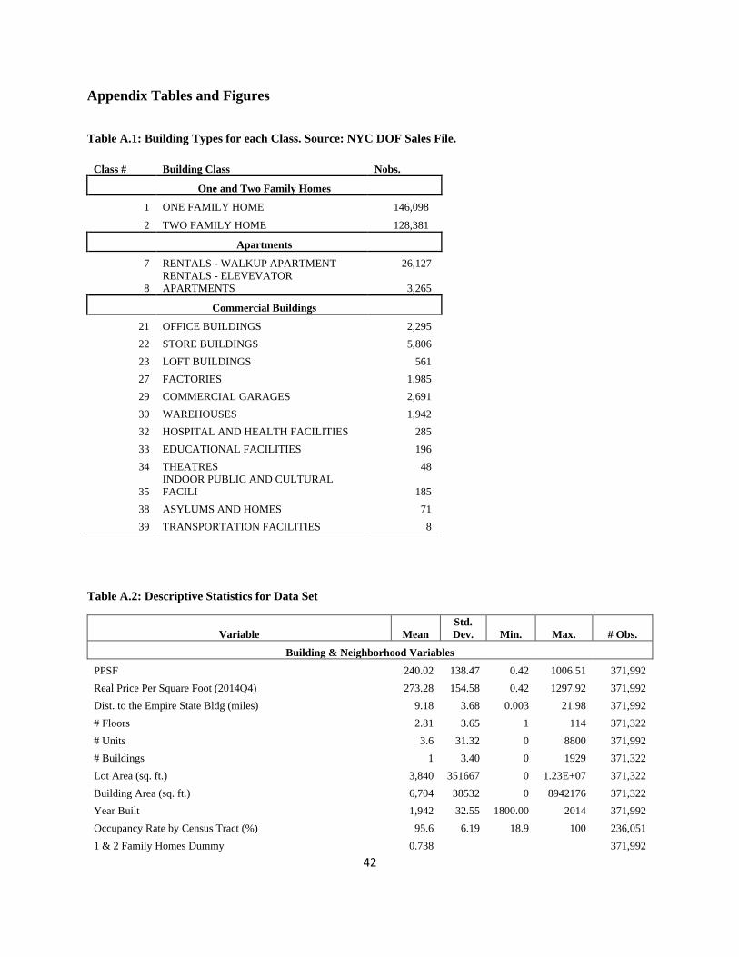
https://www.baruch.cuny.edu/confluence/display/geoportal/NYC+Mass+Transit+Spatial+Layers

42

Appendix Tables and Figures

Table A.1: Building Types for each Class. Source: NYC DOF Sales File.

Class # Building Class Nobs.

One and Two Family Homes

1 ONE FAMILY HOME 146,098

2 TWO FAMILY HOME 128,381

Apartments

7 RENTALS - WALKUP APARTMENT 26,127

8

RENTALS - ELEVEVATOR

APARTMENTS 3,265

Commercial Buildings

21 OFFICE BUILDINGS 2,295

22 STORE BUILDINGS 5,806

23 LOFT BUILDINGS 561

27 FACTORIES 1,985

29 COMMERCIAL GARAGES 2,691

30 WAREHOUSES 1,942

32 HOSPITAL AND HEALTH FACILITIES 285

33 EDUCATIONAL FACILITIES 196

34 THEATRES 48

35

INDOOR PUBLIC AND CULTURAL

FACILI 185

38 ASYLUMS AND HOMES 71

39 TRANSPORTATION FACILITIES 8

Table A.2: Descriptive Statistics for Data Set

Variable Mean

Std.

Dev. Min. Max. # Obs.

Building & Neighborhood Variables

PPSF 240.02 138.47 0.42 1006.51 371,992

Real Price Per Square Foot (2014Q4) 273.28 154.58 0.42 1297.92 371,992

Dist. to the Empire State Bldg (miles) 9.18 3.68 0.003 21.98 371,992

# Floors 2.81 3.65 1 114 371,322

# Units 3.6 31.32 0 8800 371,992

# Buildings 1 3.40 0 1929 371,322

Lot Area (sq. ft.) 3,840 351667 0 1.23E+07 371,322

Building Area (sq. ft.) 6,704 38532 0 8942176 371,322

Year Built 1,942 32.55 1800.00 2014 371,992

Occupancy Rate by Census Tract (%) 95.6 6.19 18.9 100 236,051

1 & 2 Family Homes Dummy 0.738 371,992

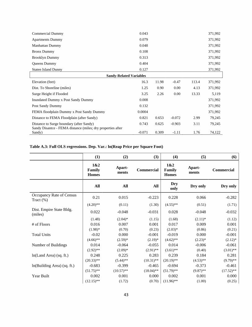
43

Commercial Dummy 0.043 371,992

Apartments Dummy 0.079 371,992

Manhattan Dummy 0.048 371,992

Bronx Dummy 0.108 371,992

Brooklyn Dummy 0.313 371,992

Queens Dummy 0.404 371,992

Staten Island Dunny 0.127 371,992

Sandy-Related Variables

Elevation (feet) 16.3 11.98 -0.47 113.4 371,992

Dist. To Shoreline (miles) 1.25 0.90 0.00 4.13 371,992

Surge Height if Flooded 3.25 2.26 0.00 13.33 5,119

Inundated Dummy x Post Sandy Dummy 0.008 371,992

Post Sandy Dummy 0.132 371,992

FEMA floodplain Dummy x Post Sandy Dummy 0.0004 371,992

Distance to FEMA Floodplain (after Sandy) 0.821 0.653 -0.072 2.99 79,245

Distance to Surge boundary (after Sandy) 0.743 0.625 -0.903 3.11 79,245

Sandy Disantce - FEMA distance (miles; dry properties after

Sandy) -0.071 0.309 -1.11 1.76 74,122

Table A.3: Full OLS regressions. Dep. Var.: ln(Reap Price per Square Foot)

(1) (2) (3) (4) (5) (6)

1&2

Family

Homes

Apart-

ments Commercial

1&2

Family

Homes

Apart-

ments Commercial

All All All Dry

only Dry only Dry only

Occupancy Rate of Census

Tract (%) 0.21 0.015 -0.223 0.228 0.066 -0.282

(4.20)** (0.11) (1.30) (4.55)** (0.51) (1.71)

Dist. Empire State Bldg.

(miles) 0.022 -0.048 -0.031 0.028 -0.048 -0.032

(1.48) (2.04)* (1.15) (1.68) (2.11)* (1.12)

# of Floors 0.016 0.007 0.001 0.017 0.009 0.001 (1.98)* (0.70) (0.23) (2.03)* (0.86) (0.21)

Total Units -0.02 0.000 -0.001 -0.019 0.000 -0.001 (4.66)** (2.59)* (2.19)* (4.62)** (2.23)* (2.12)*

Number of Buildings 0.014 -0.064 -0.055 0.014 -0.006 -0.061 (2.92)** (2.09)* (2.91)** (3.61)** (0.40) (3.01)**

ln(Land Area) (sq. ft.) 0.248 0.225 0.283 0.239 0.184 0.281 (20.33)** (5.44)** (10.31)** (20.19)** (4.53)** (9.79)**

ln(Building Area) (sq. ft.) -0.683 -0.399 -0.465 -0.694 -0.373 -0.461 (51.75)** (10.57)** (18.04)** (51.79)** (9.87)** (17.52)**

Year Built 0.002 0.001 0.000 0.002 0.001 0.000 (12.15)** (1.72) (0.70) (11.96)** (1.00) (0.25)

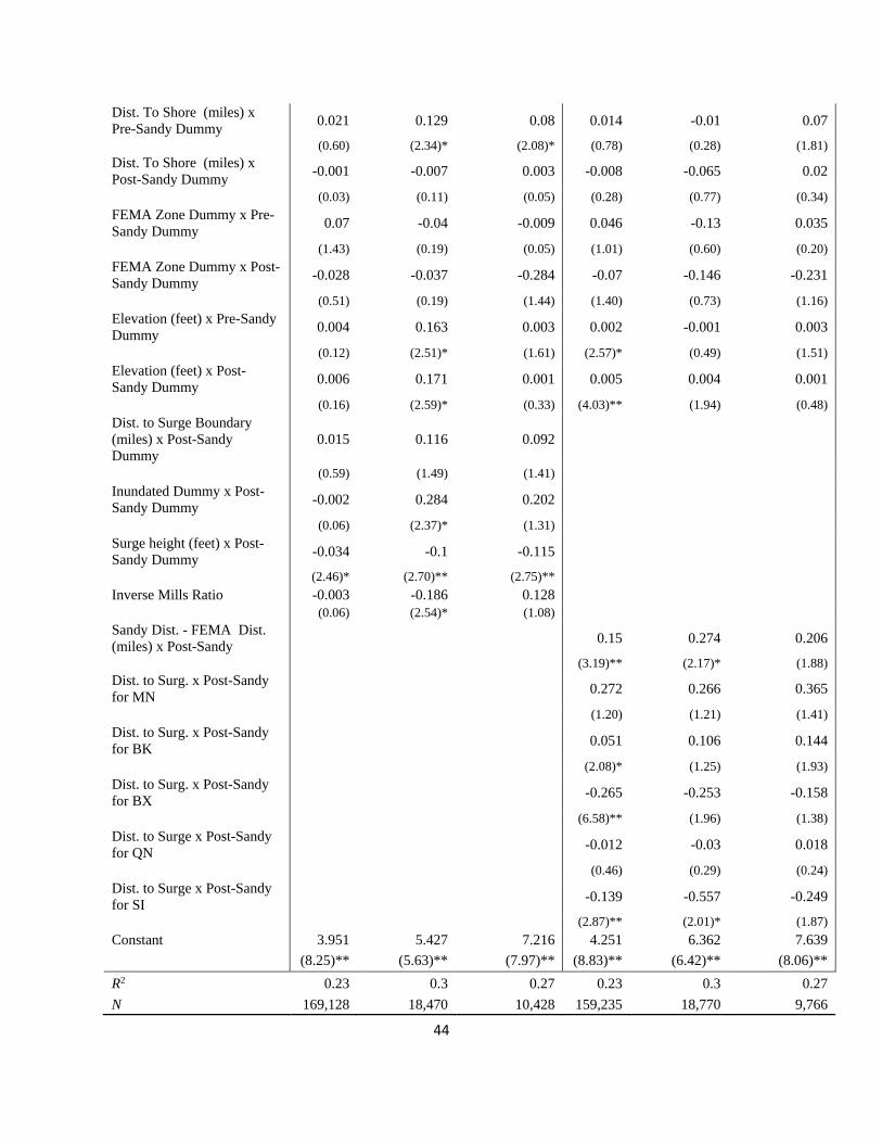
44

Dist. To Shore (miles) x

Pre-Sandy Dummy 0.021 0.129 0.08 0.014 -0.01 0.07

(0.60) (2.34)* (2.08)* (0.78) (0.28) (1.81)

Dist. To Shore (miles) x

Post-Sandy Dummy -0.001 -0.007 0.003 -0.008 -0.065 0.02

(0.03) (0.11) (0.05) (0.28) (0.77) (0.34)

FEMA Zone Dummy x Pre-

Sandy Dummy 0.07 -0.04 -0.009 0.046 -0.13 0.035

(1.43) (0.19) (0.05) (1.01) (0.60) (0.20)

FEMA Zone Dummy x Post-

Sandy Dummy -0.028 -0.037 -0.284 -0.07 -0.146 -0.231

(0.51) (0.19) (1.44) (1.40) (0.73) (1.16)

Elevation (feet) x Pre-Sandy

Dummy 0.004 0.163 0.003 0.002 -0.001 0.003

(0.12) (2.51)* (1.61) (2.57)* (0.49) (1.51)

Elevation (feet) x Post-

Sandy Dummy 0.006 0.171 0.001 0.005 0.004 0.001

(0.16) (2.59)* (0.33) (4.03)** (1.94) (0.48)

Dist. to Surge Boundary

(miles) x Post-Sandy

Dummy

0.015 0.116 0.092

(0.59) (1.49) (1.41)

Inundated Dummy x Post-

Sandy Dummy -0.002 0.284 0.202

(0.06) (2.37)* (1.31)

Surge height (feet) x Post-

Sandy Dummy -0.034 -0.1 -0.115

(2.46)* (2.70)** (2.75)**

Inverse Mills Ratio -0.003 -0.186 0.128 (0.06) (2.54)* (1.08)

Sandy Dist. - FEMA Dist.

(miles) x Post-Sandy 0.15 0.274 0.206

(3.19)** (2.17)* (1.88)

Dist. to Surg. x Post-Sandy

for MN 0.272 0.266 0.365

(1.20) (1.21) (1.41)


for BK 0.051 0.106 0.144

(2.08)* (1.25) (1.93)


for BX -0.265 -0.253 -0.158

(6.58)** (1.96) (1.38)

Dist. to Surge x Post-Sandy

for QN -0.012 -0.03 0.018

(0.46) (0.29) (0.24)

Dist. to Surge x Post-Sandy

for SI -0.139 -0.557 -0.249

(2.87)** (2.01)* (1.87)

Constant 3.951 5.427 7.216 4.251 6.362 7.639

(8.25)** (5.63)** (7.97)** (8.83)** (6.42)** (8.06)**

R2 0.23 0.3 0.27 0.23 0.3 0.27

N 169,128 18,470 10,428 159,235 18,770 9,766

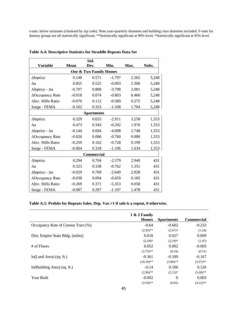
45

t-stats. below estimates (clustered by zip code). Note year-quarterly dummies and building class dummies included. F-stats for

dummy groups are all statistically significant. **Statistically significant at 99% level; *Statistically significant at 95% level.

Table A.4: Descriptive Statistics for Straddle Repeats Data Set

Variable Mean

Std.

Dev. Min. Max. Nobs.

One & Two Family Homes

∆lnprice 0.148 0.571 -1.797 2.262 5,248

∆α 0.855 0.525 -0.093 2.306 5,248

∆lnprice - ∆α -0.707 0.808 -3.798 2.001 5,248

∆Occupancy Rate -0.018 0.074 -0.803 0.466 5,248

∆Inv. Mills Ratio -0.070 0.112 -0.589 0.275 5,248

Surge - FEMA -0.102 0.353 -1.108 1.704 5,248

Apartments

∆lnprice 0.329 0.655 -2.911 3.258 1,553

∆α 0.473 0.343 -0.202 1.976 1,553

∆lnprice - ∆α -0.144 0.694 -4.098 2.748 1,553

∆Occupancy Rate -0.026 0.086 -0.760 0.086 1,553

∆Inv. Mills Ratio -0.250 0.162 -0.728 0.199 1,553

Surge - FEMA -0.064 0.318 -1.106 1.634 1,553

Commercial

∆lnprice 0.294 0.704 -2.579 2.940 431

∆α 0.323 0.338 -0.762 1.351 431

∆lnprice - ∆α -0.029 0.769 -2.649 2.928 431

∆Occupancy Rate -0.038 0.094 -0.659 0.185 431

∆Inv. Mills Ratio -0.269 0.371 -5.353 0.058 431

Surge - FEMA -0.087 0.297 -1.107 1.478 431

Table A.5: Probits for Repeats Sales. Dep. Var.=1 if sale is a repeat, 0 otherwise.

1 & 2 Family

Homes Apartments Commercial

Occupancy Rate of Census Tract (%) -0.64 -0.602 -0.233 (2.92)** (2.47)* (1.24)

Dist. Empire State Bldg. (miles) 0.018 0.027 0.009

(2.18)* (2.19)* (1.47)

# of Floors 0.052 0.002 -0.003 (2.75)** (0.19) (0.51)

ln(Land Area) (sq. ft.) -0.361 -0.189 -0.167 (10.29)** (3.86)** (5.97)**

ln(Building Area) (sq. ft.) -0.14 0.106 0.126 (2.96)** (2.13)* (5.00)**

Year Built -0.002 0 0.003 (2.93)** (0.05) (4.22)**

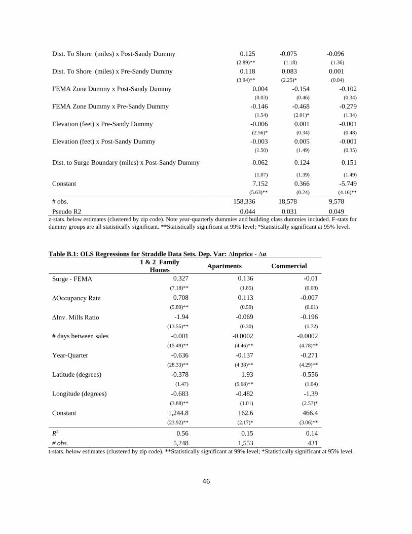
46

Dist. To Shore (miles) x Post-Sandy Dummy 0.125 -0.075 -0.096 (2.89)** (1.18) (1.36)

Dist. To Shore (miles) x Pre-Sandy Dummy 0.118 0.083 0.001 (3.94)** (2.25)* (0.04)

FEMA Zone Dummy x Post-Sandy Dummy 0.004 -0.154 -0.102 (0.03) (0.46) (0.34)

FEMA Zone Dummy x Pre-Sandy Dummy -0.146 -0.468 -0.279 (1.54) (2.01)* (1.34)

Elevation (feet) x Pre-Sandy Dummy -0.006 0.001 -0.001 (2.56)* (0.34) (0.48)

Elevation (feet) x Post-Sandy Dummy -0.003 0.005 -0.001 (1.50) (1.49) (0.35)

Dist. to Surge Boundary (miles) x Post-Sandy Dummy -0.062 0.124 0.151

(1.07) (1.39) (1.49)

Constant 7.152 0.366 -5.749

(5.63)** (0.24) (4.16)**

# obs. 158,336 18,578 9,578

Pseudo R2 0.044 0.031 0.049 z-stats. below estimates (clustered by zip code). Note year-quarterly dummies and building class dummies included. F-stats for

dummy groups are all statistically significant. **Statistically significant at 99% level; *Statistically significant at 95% level.

Table B.1: OLS Regressions for Straddle Data Sets. Dep. Var: ∆lnprice - ∆α

1 & 2 Family

Homes Apartments Commercial

Surge - FEMA 0.327 0.136 -0.01 (7.18)** (1.85) (0.08)

∆Occupancy Rate 0.708 0.113 -0.007 (5.89)** (0.59) (0.01)

∆Inv. Mills Ratio -1.94 -0.069 -0.196 (13.55)** (0.30) (1.72)

# days between sales -0.001 -0.0002 -0.0002 (15.49)** (4.46)** (4.78)**

Year-Quarter -0.636 -0.137 -0.271 (28.33)** (4.38)** (4.29)**

Latitude (degrees) -0.378 1.93 -0.556 (1.47) (5.68)** (1.04)

Longitude (degrees) -0.683 -0.482 -1.39 (3.88)** (1.01) (2.57)*

Constant 1,244.8 162.6 466.4

(23.92)** (2.17)* (3.06)**

R2 0.56 0.15 0.14

# obs. 5,248 1,553 431

t-stats. below estimates (clustered by zip code). **Statistically significant at 99% level; *Statistically significant at 95% level.

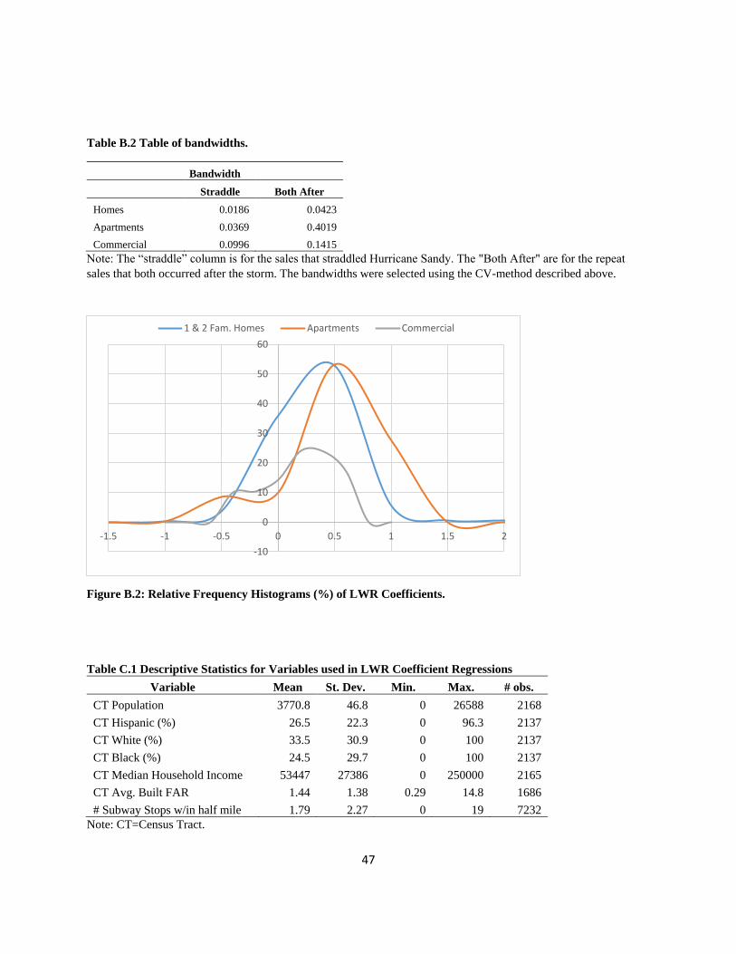
47

Table B.2 Table of bandwidths.

Bandwidth

Straddle Both After

Homes 0.0186 0.0423

Apartments 0.0369 0.4019

Commercial 0.0996 0.1415

Note: The “straddle” column is for the sales that straddled Hurricane Sandy. The "Both After" are for the repeat

sales that both occurred after the storm. The bandwidths were selected using the CV-method described above.

Figure B.2: Relative Frequency Histograms (%) of LWR Coefficients.

Table C.1 Descriptive Statistics for Variables used in LWR Coefficient Regressions

Variable Mean St. Dev. Min. Max. # obs.

CT Population 3770.8 46.8 0 26588 2168

CT Hispanic (%) 26.5 22.3 0 96.3 2137

CT White (%) 33.5 30.9 0 100 2137

CT Black (%) 24.5 29.7 0 100 2137

CT Median Household Income 53447 27386 0 250000 2165

CT Avg. Built FAR 1.44 1.38 0.29 14.8 1686

# Subway Stops w/in half mile 1.79 2.27 0 19 7232

Note: CT=Census Tract.

-10

0

10

20

30

40

50

60

-1.5 -1 -0.5 0 0.5 1 1.5 2

1 & 2 Fam. Homes Apartments Commercial

Storm Surges, Informational Shocks, and the Price of Urban ......Storm Surges, Informational Shocks,...

Documents

Transcript of Storm Surges, Informational Shocks, and the Price of Urban ......Storm Surges, Informational Shocks,...