Stock Price Synchronicity and Liquidity

Kalok Chan

Allaudeen Hameed

Wenjin Kang

2012 May * Chan is from the Department of Finance, Hong Kong University of Science and Technology, ClearWaterBay, Hong Kong, kachan@ust.hk. Hameed is from the Department of Finance, National University of Singapore, Singapore 117592, Allaudeen@nus.edu.sg. Kang is from the Department of Finance, National University of Singapore, Singapore 117592, bizkwj@nus.edu.sg. Chan acknowledges the financial support from General Research Fund of the Research Grants of Hong Kong (HKUST640308). Hameed and Kang gratefully acknowledge financial support from NUS Academic Research Grants. We thank Tarun Chordia, Gunter Strobl, Avanidhar Subrahmanyam, an anonymous referee, and seminar participants at Manchaster University, Nomura (Tokyo), Lancaster University, Tsinghua University, 2008 WFA Meetings (Hawaii), 2008 China International Conference in Finance (Dalian), 2008 NFA AsianFA Meetings and 4th Annual Central Bank Workshop on the Microstructure of Financial Markets Hong Kong SARfor useful comments.

Stock Price Synchronicity and Liquidity

Abstract

We argue and provide evidence that stock price synchronicity affects stock liquidity. Under the “relative synchronicity” hypothesis, higher return co-movement (i.e. higher systematic volatility relative to total volatility) improves liquidity. Under the “absolute synchronicity” hypothesis, stocks with higher beta or systematic volatility are more liquid. Our results support both hypotheses. We find all three liquidity measures (effective proportional bid-ask spread, price impact measure and Amihud’s illiquidity measure) are positively related to stock return co-movement and decrease with systematic volatility. Besides market co-movement, larger industry wide component in returns also improves liquidity. We also find that improvement in liquidity following additions to the S&P 500 indexis related to the stock’s increase in return co-movement.

1

Liquidity reflects the ability to trade large quantities of a security quickly, with minimal

trading costs and little price impact. Extensive research has been conducted in understanding the

cross-sectional and time-series variation of liquidity in the equity market. A key determinant of

liquidity is the volatility of underling stocks. An increase in volatility of underlying stock returns

implies that the liquidity providers will face higher adverse selection risk due to increased

possibility of trading with informed investors as well as higher inventory risk arising from order

imbalances. As a result, higher asset price volatility leads to lower asset liquidity (see, for

example, Stoll (1978), Ho and Stoll (1981), and Stoll (2000)).

While existing studies show that an increase in volatility lowers liquidity, there is little

research work on the separate effects of systematic volatility and idiosyncratic volatility on

liquidity. According to the adverse selection models or inventory risk models, the effect of

systematic volatility on liquidity should be different from that of idiosyncratic volatility, given that

systematic risk can be hedged to a certain extent. Furthermore, Baruch, Karolyi and Lemmon

(2007) and Baruch and Saar (2009), for example, argue that stock return co-movement affects the

trading activity of a stock and therefore its liquidity. This is because the correlation of stock

returnswith the market measures the amount of market-wide information relative to firm-specific

information. While market makers can observe the market-wide information easily, it is more

difficult for them to observe firm-specific information. When an individual stock is highly

correlated with the market, market makers can rely more on the information he observes from the

market movement so that the stock price adjustments are less sensitive to its own order flow.

Consequently, both liquidity and informed traders choose to trade a larger proportion of the cross-

listed asset in the exchange with the higher return correlation with the domestic assets. That is,

proportionally more volume migrates to the market in which the cross-listed asset has greater

correlation with the other assets traded on the market.1Moreover, Subrahmanyam (1991)

demonstrates that the introduction of basket of securities provides a preferred trading medium for

uninformed liquidity traders, because adverse selection costs are typically lower in these markets

than in markets for individual securities. This is related to the idea that the basket of securities is

1 Bhushan (1991) and Caballe and Krishnan (1994) also show the market maker is able to extract greater

amount of information from the order flow of the other securities when the stock co-moves more with the

market.

2

affected mostly by systematic returns, as security specific returns are diversified away, and

consequently, are more liquid.

We test for two empirical hypotheses in this paper. Our first hypothesis is the “relative

synchronicity” hypothesis which predicts that stock return co-movement, or the r-squared measure,

positively affects the liquidity of a stock, as market makers learn more information from the

market if the stock has more correlated fundamentals. The second hypothesis is the “absolute

synchronicity” hypothesis which predicts that idiosyncratic volatility and systematic volatility have

different effects on liquidity, as market makers can hedge away systematic risk to a certain

extent.Since a higher amount of market-wide information lowers the adverse selection risk, we

expect that an increase in systematic volatility to be accompanied by an improvement in liquidity.

We conduct empirical analysis based on a sample of NYSE stocks from 1989 to 2008, and

construct various liquidity measures, including effective proportional bid-ask spread, Kyle’s price

impact measure and Amihud’s illiquidity measure.

Our empirical evidence supports both hypotheses. For the “relative synchronicity”

hypothesis, we find that stock price synchronicity, a measure of stock return co-movement, has a

negative relationship with all three liquidity measures. For the “absolute synchronicity” hypothesis,

we also find that a decrease with systematic volatility or market betaimproves stock liquidity. Our

results cannot be explained by cross-sectional differences in firm size, price levels, institutional

ownership, turnover,and idiosyncratic volatility which we use as control variables.

We argue that our results are not due to the reverse causality from liquidity to stock return

synchronicity, as there is a similar relationship between firm’s earnings co-movement and liquidity.

Our contention is that it is unlikely that stock liquidity drives the earnings synchronicity. Based on

market model regressions using accounting return on assets (ROA), we find that firms with higher

earnings co-movement have higher stock liquidity, confirming the causal effect of co-movement

on liquidity.

We also show that the co-variation in returns at the industry level is positively related to

liquidity: firms with greater industry-wide return co-movement in returns exhibit higher liquidity.

We also find a similar effect of higher industry-wide volatility and industry beta on stock liquidity.

These results support our contention that larger market or industry wide component in returns

reduces the adverse selection risk faced by the liquidity providers and hence, improves the supply

3

of liquidity. We demonstrate that the relationship between liquidity and stock price synchronicity

is related to the extent of information asymmetry. When partitioning the sample into S&P 500

stocks versus non- S&P 500 stocks, we find that the relationship is stronger for non-S&P 500

stocks that have a higher degree of information asymmetry. Our results also shed light on the

indexing effect, where firms in the major market index are likely to co-move more with the market

and experience better liquidity. In fact, we show that for firms being added to the S&P 500 index,

the improvement of the liquidity could be attributed to the increase in co-movement with the

market.

The paper is organized as follows. Section I provides a discussion of the effect of stock

price synchronicity on liquidity. In Section II we describe the data and methodology used in the

research. Section IIIcontains the basic results on relationship between liquidity and stock price

synchronicity, while Section IV contains extended analysis. Section V provides the conclusion.

I. Effect of stock price synchronicity on liquidity

Stock price synchronicity, or the R-squared measure, measures the proportion of

systematic volatility relative to the total volatility or idiosyncratic volatility. In this section, we

survey related literature and discuss the potential effects of stock price synchronicity on liquidity.

There is extensive literature that predicts a negative relationship between asset price

volatility and asset liquidity (Stoll (1978), Ho and Stoll (1981), and Stoll (2000)). Previous studies,

however, do not distinguish between systematic and idiosyncratic volatilities and examine how

each type of volatility may affect liquidity differently. Existing theories suggest that the

idiosyncratic volatility has a larger impact on liquidity than the systematic volatility. First, the

adverse selection risk primarily should come from the idiosyncratic component.This is because

while insiders or informed investors have advantages in collecting idiosyncratic (or firm-specific)

information, it is more difficult for investors to possess a similar advantage with regards to

thesystematic (or market-wide) information. Second, the inventory risk is more likely to arise from

the idiosyncratic volatility as market makers can hedge against the market risk using stock index

futures or derivative products.

4

While there are strong theoretical and empirical support for the negative association

between liquidity and idiosyncratic volatility2, very little is known about the relationship between

liquidity and systematic volatility. In theory, the inventory risk associated with the market can be

hedged completely and there is no adverse selection risk due to the market factor. In this case,

market makers do not need compensation for providing liquidity on account of systematic risk, so

that there is no effect of systematic risk on liquidity. In practice, market makers are unable to

completely eliminate the market risk in their inventory control, because hedging against market

risk is either costly or imperfect. As for the adverse selection risk, some of the private information

that an insider obtains about a company might be relevant for the market as a whole. Therefore,

even for the systematic component, the market makers need to protect themselves against adverse

selection.

A number of previous studies document commonality in liquidity (Hasbrouck and Seppi

(1998) and Huberman and Halka (1999), and Chordia, Roll and Subrahmanyam (2000)). These

papers find that there are significant co-variations in liquidity among stocks. The existence of

commonality in liquidity suggests that liquidity is driven by some common sources. For example,

program trading of simultaneous large orders will exert common pressure on dealer inventories.

Furthermore, institutional investors with similar investing styles might exhibit correlated trading

patterns, thereby inducing changes in inventory pressure across the broad market. When dealing

with a portfolio of stocks, market makers have to prepare for unexpected common pressure on

inventories in their liquidity provision. Therefore, we expect a negative impact of systematic risk

of a stock on its liquidity, although it might not be as strong as the idiosyncratic risk.

Furthermore, according to Subrahmanyam (1991), the amount of liquidity trading can be

endogenous, as there are discretionary liquidity traders who will choose to trade in securities that

have the least adverse selection risk. Since stocks of higher systematic information have less

adverse selection, discretionary liquidity traders making portfolio adjustment can minimize the

2Goyal and Santa-Clara (2003) provide empirical evidence on a positive relation between the idiosyncratic

volatility and average stock returns. Bali, Cakici, Yan, Zhang (2005), however, show that the idiosyncratic

volatility might simply proxy for liquidity, so that the empirical evidence documented in Goyal and Santa-

Clara (2003) is a reflection of liquidity premium. Spiegel and Wang (2006) also show that idiosyncratic

risk and liquidity are negatively correlated.

5

liquidity cost by concentrating their trades in these stocks, resulting in a further improvement of

liquidity.

So far, our discussion has been on the differential impact of systematic volatility and

idiosyncratic volatility on liquidity. A couple of papers (Baruch, Karolyi and Lemmon (2007))

and Baruch and Saar (2009)) examine the stock return co-movement, or the amount of market-

wide volatility relative to firm-specific volatility, and demonstrate that it affects the trading volume

and thereby the liquidity of a stock. These papers build theoretical models in which the market

maker infers information based on order flows. The higher the return co-movement of a security,

the more information the market maker is able to extract about the value of the security from the

order flows of other securities in the market. This decreases the adverse selection risks, increases

the incentives to trade the security, and lowers the sensitivity of the asset price to its own order

flow. Hence, return co-movement is positively related to liquidity of the asset. Baruch and Saar

(2009) show that a stock is more liquid when it is listed on a market where“similar” securities are

traded, or when it has a higher correlation with other securities. They find that stocks that switch

their listing from NASDAQ to the NYSE have return patterns more similar to securities already

listed on the NYSE. They also document liquidity improvements for the switching firms that are

positively related to the degree of similarity in the return patterns. Baruch, Karolyi and Lemmon

(2007) show the distribution of the trading volume across international stock exchanges is related

to the correlation of the cross-listed asset returns that arise in the respective markets. Based on a

sample of non-US stocks cross-listed on major U.S. exchanges, they find that volume migrates to

the exchange in which there is a greater correlation between the cross-listed asset returns and

returns on other assets traded in the market.

We postulate two hypotheses based on the above discussions. The first is the “relative

synchronicity” hypothesis. Under this hypothesis, stocks with a higher degree of co-movement (i.e.

a higher proportion of systematic volatility) are more liquid. The rationale for the prediction is the

learning effect as described in Baruch, Karolyi, and Lemmon (2007) and Baruch and Saar (2009),

whereby learning about the information that drives the asset’s price improves liquidity. This

hypothesis predicts a positive relationship between stock return co-movement and liquidity.

The second is the “absolute synchronicity” hypothesis. Under this hypothesis, what affects

liquidity is the amount of systematic volatility, and idiosyncratic volatility. This hypothesis

6

predicts that after holding idiosyncratic volatility constant, higher systematic volatility enhances

liquidity. We will conduct empirical tests of these two empirical hypotheses in the next section.

II. Data and Methodology

The sample consists of all NYSE traded ordinary common stocks, identified by the Center

for Research in Security Prices (CRSP) share code 10 and 11, over the period January 1989 to

December 2008. We exclude stocks traded on NASDAQ to avoid the influence of differences in

trading protocols. The CRSP dataset contains daily stock returns, daily trading volume, number of

shares outstanding, and yearly market capitalization. We filter out stocks with extreme price levels

by discarding stocks with prices below $1 and above $999. For transaction-level data, we retrieve

all trades and quotations from the New York Stock Exchange Trades and Automated Quotations

(TAQ) and the Institute for the Study of Securities Markets (ISSM).34

We construct several different proxies of firm level liquidity used in the prior literature.

The first measure of liquidity is the price-impact measure ( ) introduced in Kyle (1985). For each

firm, we use the price and quote information from TAQ to classify every trade as buyer (seller)

initiated, based on whether the transaction price is greater (lower) than the prevailing average of

bid and ask quotes. Specifically, we follow the algorithm presented in Lee and Ready (1991) in

signing the transactions as buy and sell orders, matching trading records to the most recent quote

preceding the trade by at least five seconds. We aggregate the buy and sell orders at the daily level

and compute firm i’s net order imbalance at day t, OIBi,t, defined as the difference between the

value of daily buyer and seller initiated trades.

Our estimate of for firm i is the coefficient from the following regression,

titiiiti OIBR ,,, (1)

where Ri,tisthe returns on stock i on day t. Equation (1) specifies that the stock price responds to

the net order imbalance. We have also estimated equation (1) by adding the return on the market

3 Anomalous transaction records are deleted according to the following filter rules: (i) Negative bid-ask

spread; (ii) Quoted spread > $5; (iii) Proportional quoted spread > 20%; (iv) Effective spread / Quoted

spread > 4.0. 4 We thank Tarun Chordia for sharing the TAQ based measures of liquidity for the more recent years.

7

portfolio as an explanatory variable and obtain similar results. Therefore, the effect of net order

imbalance on the stock returns, as measured by i , is not affected when we control for the effect of

market movement.

For each year t, we estimate the daily price impact coefficient i by regressing daily

returns on its corresponding order imbalance. Using a similar measure, Brennan and

Subrahmanyam (1996) find that the price impact measure of liquidity is positively related to

average stock returns, suggesting that illiquid stocks are compensated with liquidity premium.

Besides estimating i based on Equation (1), we also do the estimation using a transaction-based

measure and obtain similar results.5

Our second liquidity measure is the effective bid-ask spread. Stoll (1978), Glosten and

Harris (1988) and others show that bid-ask spreads include an adverse selection costs of the market

maker trading with investors with superior information. We calculate the proportional effective

spread based on two times the absolute difference between the trade execution price and the

midquote, divided by the midquote. The daily average proportional effective spreads for firm iare

averaged each calendar year to generate our annual spread measure (ESPRi).

The third liquidity measure is based on Amihud (2002) and does not rely on intraday

transactions data. It is calculated as the absolute daily return on stock i divided by the firm’s daily

dollar volume. Using this measure of the relative price change associated with trading volume,

Amihud finds that firms with greater expected illiquidity earn higher expected returns, consistent

with an illiquidity premium in returns. Acharya and Pedersen (2005) also use this illiquidity

measure to investigate the effect of liquidity on security returns. Hasbrouck (2005) shows that the

Amihud illiquidity measure is a robust measure of price impact as posited in Kyle (1985).

It should be noted that the three measures are in fact illiquidity measures. If a stock is less

5 We also use a transaction-based measure of Kyle’s as an alternative. Here, we follow the approach of

Brennan and Subrahmanyam (1996): let pj and qj denote the price and the signed quantity of the order

fulfilled for transaction j, and Dj denote the sign of the order. The regression

jjjTj Dqp provides the estimates for the Kyle’s T .Its common practice to use Δpj

= (pj–pj-1)/pj-1 as the regressor to ensure that our comparison of the price impact estimate across different

stocks is not affected by the price level. Our results are qualitatively similar when we use this transaction-

based measure for the period 1989-2003.

8

liquid, it will have a higher bid-ask spread, its order flow will have a larger impact on stock prices,

and the absolute price change per unit of volume is greater. Therefore, an increase of any of these

measures is an indication of lower liquidity.

To investigate the relation between liquidity and the amount of market-wide information,

we rely on the standard market model regressions to extract the market-wide component in returns.

We start with the regression of weekly stock returns on stock i at week t (Ri,t) on the CRSP value-

weighted weekly market returns (Rmkt,,t): tik

ktmktRkiatiR ,1

1,,,

, where we include one

week lead and lag of market returns to account for any delayed adjustment in stock prices to

market-wide information. Note that this is a standard market model, and does not include the net

order imbalance as the explanatory variable like Equation (1), as our primary objective here is to

distinguish return fluctuations being explained by the market from those not explained. To test the

relative synchronicity hypothesis, we use the R-squared of stock i ( 2iR ) from the market model

regression, which reflects the proportion of variation in return of stock i explained by market

return. Since the R-squared statistics is bounded between zero and one, the relative price

synchronicity of stock i (Synchi) is obtained by taking the logit-transformation of 2iR : ln( 2

iR /(1-

2iR )). A higher Synchiindicates a larger amount of market-wide information in stock i. We use

two related measures of the absoluteamount of market-wide information estimated from the

regression. The first is the stock’s beta (

1

1kk,ii ), which measures the sensitivity of return

of stock ito market return. The second measure is based on thesystematic volatility estimated

directly from the market model regression. The systematic volatility, SysVoli, is the square root of

the systematic variance of stock i, i.e. )(2mkti RVar . The corresponding idiosyncratic volatility

(IdioVoli) is given by the square root of the difference between the total variance of stock i and the

systematic variance. We investigate whether the effect of systematic volatility on liquidity is

distinct from that due to idiosyncratic volatility.

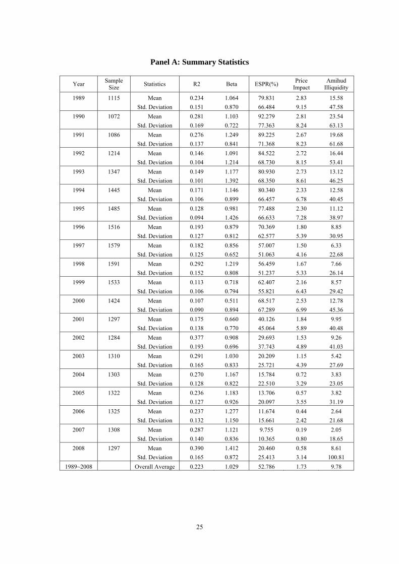
Table 1 contains summary statistics on our liquidity and price synchronicity measures for

each year from 1989 to 2008. Panel A reports the number of stocks, mean and standard deviation

of R2, stock’s beta, as well as three liquidity measures (effective bid-ask spread, price impact, and

9

Amihud illiquidity measure). If we include all the stocks, the betas should average to about one.

But since our sample, which ranges between 1072 and 1591 stocks per year, excludes NASDAQ

stocks that tend to have higher betas, the average beta of our NYSE stocks is below one in a

number of years, especially during the technology bubble period from 1999 to 2001. On the other

hand, during the market turmoil of 2008, our sample stocks co-move with the market significantly,

with an average beta of 1.412. The R-squared from the market model regression averages to about

22.3 percent over the whole sample period, with yearly averages in the range of 10.7 percent to

39.0 percent. All three liquidity measures display a downward trend in illiquidity over time. For

example, the effective bid-ask spread is 0.798%, 0.923%, and 0.894% in the first three years, and

declines steadily during the sample period to 0.137%, 0.116%, and 0.097% in 2005-07, before it

widens during the financial crisis of 2008. . The other two liquidity measures also have a similar

pattern, although the decline is less pronounced. Over the sample period, the price impact measure

declined from 2.83and hit the lowest point of 0.19 in 2007, while the Amihud illiquidity measure

declined from 15.58and hit the lowest point of 2.05 in 2007. Panel A also presents the cross-

sectional standard deviations. The price impact and Amihud illiquidity measures exhibit

substantial cross-sectional dispersion, as their standard deviations are more than 3 times larger than

the mean values.

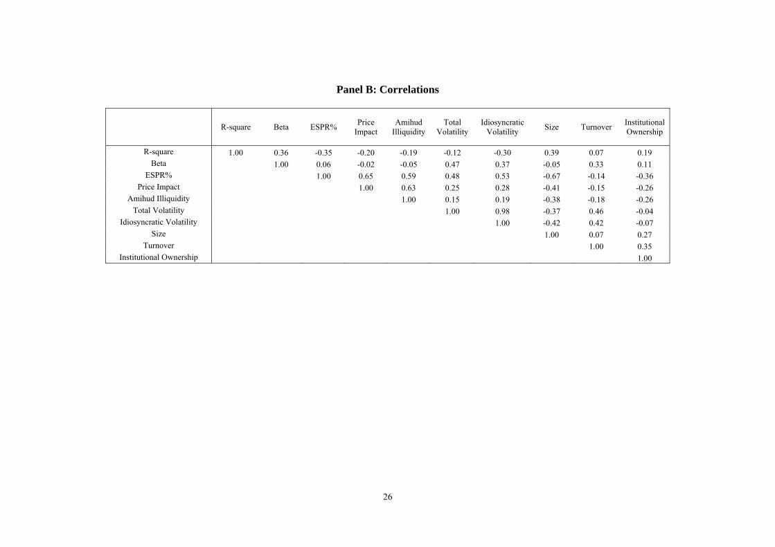
Panel B of Table 1 reports the unconditional correlations across firm-years among R-

squared, beta, the liquidity proxies, and other firm specific characteristics that we use as control

variables. In general, all the liquidity measures are highly correlated with each other, a result

consistent with Korajczyk and Sadka (2005) and Hasbrouck (2009). We find that the daily price

impact coefficient is highly correlated with both the effective spread andAmihud illiquidity.

The R-squared measure is highly correlated stock’s beta and idiosyncratic volatility, with a

correlation coefficient of 36% and -30%, respectively. It is noted that the correlation of total

volatility with idiosyncratic volatility is 98%, and therefore the cross-sectional variation of firm

volatility is primarily driven by the firm-specific component. Finally, the correlation of liquidity

measures with idiosyncratic volatility is higher than the correlations with the total volatility,

providing preliminary evidence of the asymmetric effect of systematic volatility and idiosyncratic

10

volatility on the liquidity.

III. Empirical Relationship Between Liquidity and Stock Price Synchronicity

A. Explanatory Variables

Several studies show that cross-security variation in liquidity can be explained by firm

characteristics. Stoll (1978, 2000), Ho and Stoll (1981) and Harris (1994) show that proportional

bid-ask spreads are lower for bigger firms and high volume stocks as they are associated with

higher probability of finding a counterparty to trade and hence are associated with lower inventory

and order processing costs faced by the market maker. They also show that spreads are higher for

stocks with high return variance due to compensation for inventory risks as well as the risk of

trading with an informed trader. Hasbrouck (1991) reports that the price impact (and adverse

selection risk) is higher for smaller firms. Breen, Hodrick and Korajczyk (2002) show that the

price impact of trade is related to a number of firm specific variables, including firm’s market

capitalization, volume, absolute returns, and institutional ownership.

To test for the “relative synchronicity” hypothesis, we regress our liquidity measures on

the proportion of systematic information in stock returns, measured by stock return synchronicity

(Synch). To test for “absolute synchronicity” hypothesis, we have a couple of empirical

specifications. One specification incorporates both idiosyncratic volatility (IdioVol) and

systematic volatility (SysVol) as explanatory variables in the regression model, so that we can

directly compare their distinct effects on liquidity. In another specification, we use beta to

measure the absolute amount of systematic information, while controlling for idiosyncratic

volatility (IdioVol) in the regression model. The beta measure provides us with an alternative

functional form in measuring systematic risk.

We introduce a set of control variables that other studies have shown to affect firm level

liquidity, independent of the amount of market-wide information. The first is firm size (SIZE),

which is equal to the log of market capitalization at the beginning of the year. Firm size is a proxy

for adverse selection risk, which might affect the liquidity of the stock. The second variable is the

institutional ownership (IO), or the percentage of the firm’s equity held by institutional investors.

For each year, the institutional holdings are measured as of the end of the previous year. Since a

higher institutional ownership is accompanied by more information disclosure and lower adverse

11

selection risk, it should be accompanied by higher stock liquidity. The third is turnover, which is

the ratio of daily trading volumeto the number of shares outstanding, averaged over the year. By

construction, since turnover is endogenously determined, it might capture the influences of other

variables that explain our liquidity measures. Therefore, the effect of our synchronicity measures

on the liquidity measures might be understated. The fourth variable is the inverse of price (1/P),

where P is the beginning of year price for the firm. When liquidity is measured by proportional

effective spread, it is possible that the cross-sectional variation in liquidity is affected by

differences in the price levels. Hence, we include the inverse of price as a control variable if the

dependent variable is proportional effective spread.

B. Basic Empirical Results

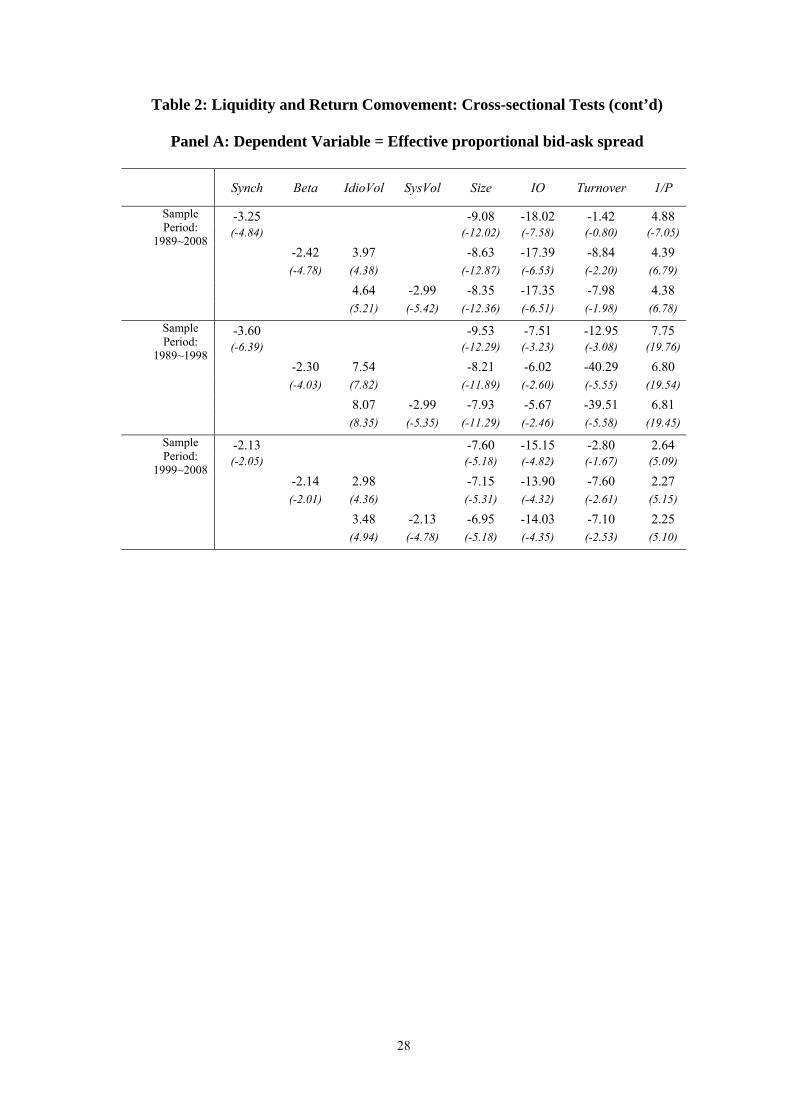
Table 2 presents the results of the cross-sectional analysis, based on the fixed-effect panel

regression, controlling for the time-trend in our liquidity measures. Panel A contains the results

using effective proportional bid-ask spread as the dependent variable. The t-statistics, contained in

parenthesis, are calculated using robust standard errors adjusted for firm and year clustering (see

Petersen (2009)). Results for the control variables are consistent with our conjecture.

Proportional bid-ask spreads are negatively related to firm size, institutional ownership, turnover,

and positively related to inverse of price level.

There is strong evidence in support of the “relative synchronicity” hypothesis. In the first

specification, the synchronicity measure (Synch) is strongly and negatively related to the effective

bid-ask spread. Therefore, an increase in the proportion of market-wide information in the stock

prices increases its liquidity (lower bid-ask spread). There is also supporting evidence for the

“absolute synchronicity” hypothesis. In the second specification, effective bid-ask spread is

negatively related to the amount of systematic information based on Beta, and positively related to

the idiosyncratic volatility (IdioVol). In the third specification, , when we decompose the total

risk into idiosyncratic volatility (IdioVol) and systematic volatility (SysVol), we find that the two

volatilities have opposite effects on liquidity. While an increase in idiosyncratic volatility

increases the bid-ask spread, an increase of systematic volatility decreases it. Therefore, instead of

adversely affecting the liquidity, an increase in market-wide information actually attracts more

liquidity trading, resulting in lower bid-ask spread. We have also partitioned the sample period

12

into two sub-periods. We continue to find a negative relation between bid-ask spreads and

synchronicity (measured by R-squared or beta), as well as different impacts of systematic volatility

and idiosyncratic volatility on liquidity.

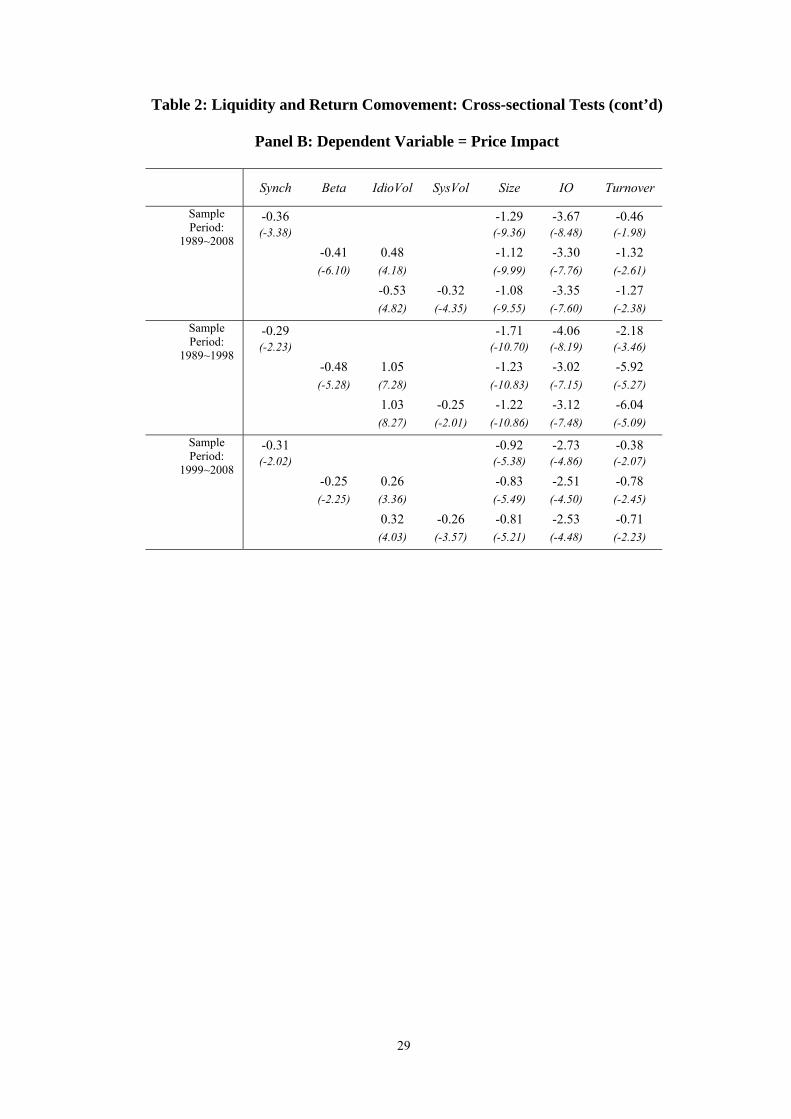
Panel B of Table 2 contains the results using the price impact coefficient as the dependent

variable. Results are similar to those based on the effective bid-ask spread. Consistent with the

“relative synchronicity” hypothesis, there is a significantly negative relationship between price

impact and price synchronicity, indicating that price impact of trades is smaller for stocks with

higher co-movement with the market. Also consistent with the “absolute synchronicity:

hypothesis, the price impact coefficient is negatively related to beta, once the idiosyncratic

volatility is controlled for. Finally, the effects of idiosyncratic volatility and systematic volatility

are asymmetric. While an increase in idiosyncratic volatility increases the price impact coefficient,

an increase of systematic volatility decreases it. The results are again robust in all three sub-

periods.

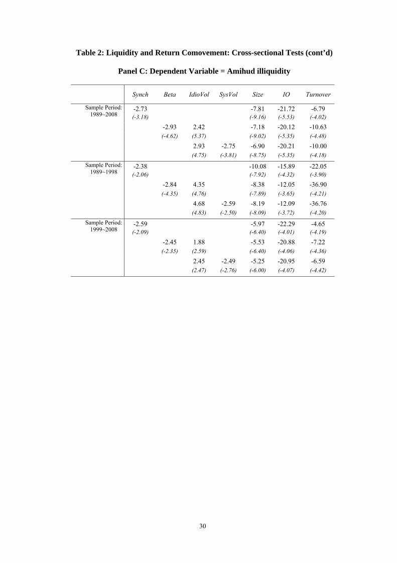
Similar findings are obtained when we use Amihud illiquidity as the dependent variable,

which are reported in Panel C of Table 2. Amihud illiquidity is lower for firms with higher stock

return synchronicity. It is also lower for stocks of higher systematic volatility, and higher betas,

after controlling for the idiosyncratic volatility. We also obtain similar results in the sub-period

analysis. .

Since our Synchmeasure reflects the proportion of individual stock returns explained by

the market, one might wonder whether there is a mechanical relationship between Synch and the

liquidity measure as measured by the price impact coefficient ( ). Based on Equation (1), a

larger implies that a smaller percentage of stock returns is attributable to the market and

therefore a lower R2. It should be noted that when we re-estimate the price-impact measure

including market returns as the explanatory variable and obtain similar results. Furthermore,

besides the price impact coefficient, we have two other liquidity measures (bid-ask spread and

Amihud illiquidity), which are estimated independent of the market model. These two liquidity

measures are unlikely to be affected by any mechanical relationship embedded in equation (1).

We will also conduct additional analysis to show that our results are not due to any mechanical

relationship.

In an unreported table available upon request, we apply the test statistics from Plosser,

13

Schwert, and White (1982) to compare the inference from the three regression specifications. The

PSW test is applied to each stock in our sample and we fail to reject the null hypothesis that the

model is correctly specified for most of the stocks. When we measure liquidity using bid-ask

spreads, we do not reject the null hypothesis for 87 to 91 percent of firms across the three model

specifications. Similarly, we fail to reject the PSW specification test for more than 84 percent of

the firms when liquidity is computed based on the price impact, and 82 percent of the firms when

liquidity is computed based on Amihud illiquidity. This provides support for both the absolute

synchronicity hypothesis and the relative synchronicity hypothesis.

C. Robustness Tests

C.1Results based on changes in stock price synchronicity

One explanation for our findings is that stock price synchronicity reflects some firm

characteristics being correlated with liquidity, other than firm size, institutional ownership and

turnover that we control for in the regression analysis. The relationship between illiquidity and

stock price co-movement or systematic volatility could be a reflection of omitted firm

characteristics. As a robustness check, we employ an alternative set of empirical specifications

investigating the relationship using changes in liquidity and changes in explanatory variables. Each

year, we compute changes in stock return synchronicity, beta, systematic volatility, idiosyncratic

volatility, as well as changes in control variables, and estimate the following specifications for the

cross-sectional time-series observations:

t,ik

t,ik

ktt,it,i CONTROLSynchbaLiquidity (2)

t,ik

kt,i

ktt,it,it,i CONTROLIdioVolcBetabaLiquidity (3)

tik

kti

kttititi CONTROLIdioVolcSysVolbaLiquidity ,,,,, (4)

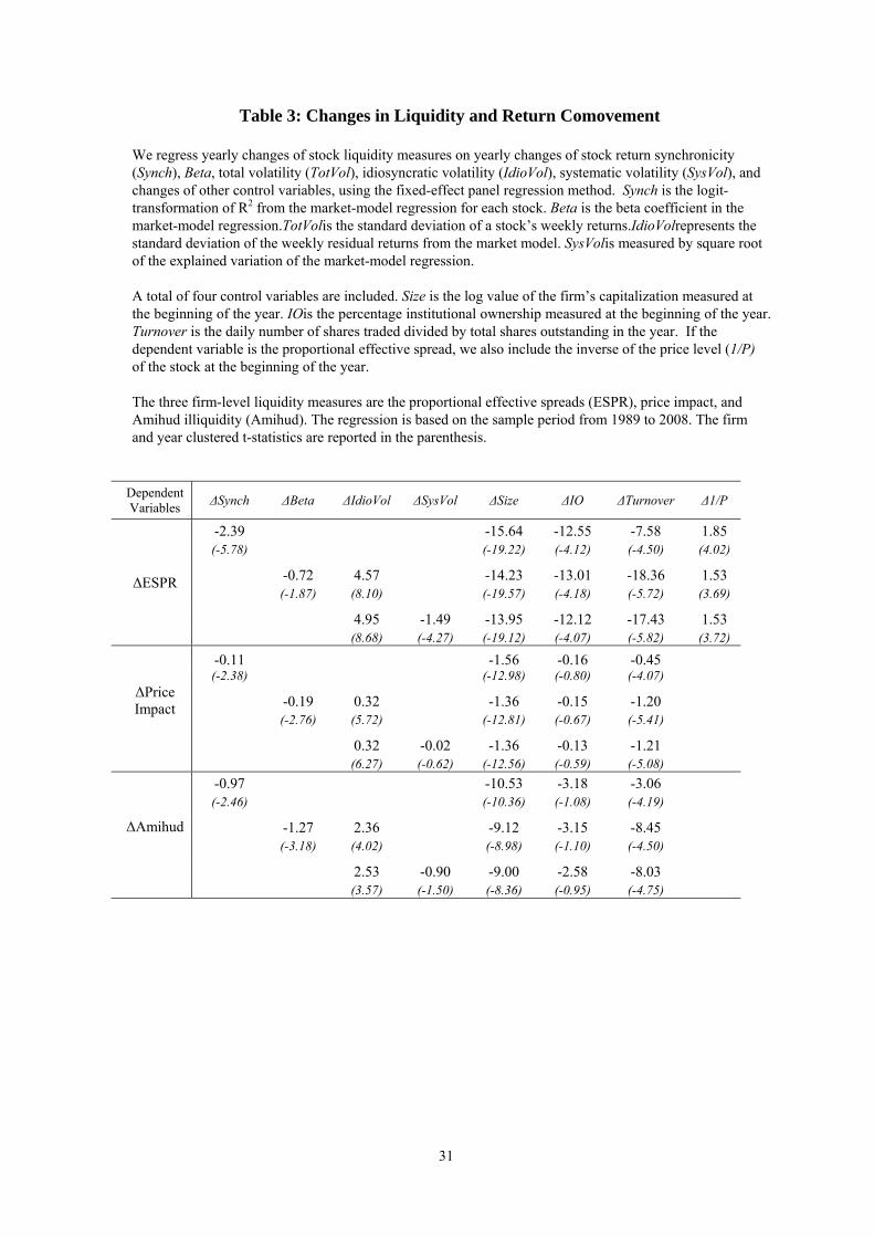
Results are reported in Table 3. Consistent with our regression results using the levels, we

find that changesin stock price synchronicity ( Synch ) is negativelyrelated to changesof liquidity

measures, regardless of whether effective spreads, price impact and Amihud illiquidity measures

are used. In other words, after a firm experiences an increase in stock price synchronicity, the

stock will experience an improvement in liquidity. This evidence is in support of the relative

synchronicity hypothesis.In the second specification, after controlling for the change of

14

idiosyncratic volatility ( IdioVol ), the change in beta ( Beta ) is negatively correlated with our

illiquidity variables. Therefore, the result also supports the absolute synchronicity hypothesis.

The third specification uses the change in SysVol ( SysVol ) and we obtain similar evidence only

when liquidity is measured by change in spreads. We obtain less statistically significant results

when we use change in Amihud illiquidity or a change in price impact measures. In the latter

specifications, the change of idiosyncratic volatility ( IdioVol ) remains statistically significant,

but the change of systematic volatility is not. Overall, the negative relationship between illiquidity

and stock price synchronicity also holds using changes in the explanatory variables, with stronger

support for the relative synchronicity hypothesis.

C.2 Results based on frequently traded stocks

Another explanation for the evidence that illiquid stocks have lower co-movement with the

market is that betas are underestimated due to thin trading problem. For those illiquid stocks that

have higher bid-ask spread, higher price impact and higher Amihud illiquidity, they will tend to

have lower beta and lower systematic volatility. We do not think that such an explanation is likely,

as our beta and R-squared estimates already adjust for delayed adjustments due to thin or non-

synchronous trading using the leading and lagging market returns.

Besides the thin trading, if large price impact and transaction costs discourage trading, this

can give rise to another mechanism through which the liquidity affects the stock return

synchronicity. Here, large transaction costs deter arbitrageurs from trading in the stock, while

other stocks are moving due to common information. Consequently, for these illiquid stocks, their

prices adjust only to large deviations from fundamental values, and hence, their synchronicity with

the market will be lower. As a robustness test, Panel A of Table 4 presents additional analysis

based on stocks that do not have any zero trading volume days in the year. In this way, we

eliminate the illiquid stocks and conduct our investigation on stocks that are less prone to the

infrequent trading problem. We also examine the impact of removing stocks that have low number

of trades each day, and require that stocks have at least an average of 10 trades per day. The

results are presented in Panel B of Table 4. Results in Table 4 are generally similar to those in

Table 2, except that the relation between Amihud illiquidity and systematic volatility becomes less

significant, weakening the support for the absolute synchronicity hypothesis.

15

D. Results based on earnings co-movement

It is possible that the relationship we observe in Table 2 may not necessarily reflect

causality running from stock return synchronicity or systematic volatility to liquidity. Instead, one

can imagine a mechanism for the reverse causality from liquidity to stock return synchronicity.

For example, liquid stocks are more likely to trade first upon the arrival of market-wide

information, so that the more liquid stocks will have a higher return co-movement with the market,

resulting in a higher R2. Furthermore, even if there is no reverse causality from liquidity to return

synchronicity, there might be missing factors that simultaneously drive both liquidity and return

synchronicity. For example, some stocks are more prone to investor sentiment, so that when the

sentiment is high, there are a lot more trading for these stocks (Baker and Stein (2004)), which also

experience higher stock return synchronicity (Barberis, Shleifer and Wurgler (2005)). To

summarize, since it is possible that stock return synchronicity is endogenously determined, either

by liquidity or other missing factors, one cannot ascertain if the empirical relationship that we

report really reflects the effect of synchronicity on liquidity.

To address this issue, we construct co-movement measures based on accounting earnings

as an instrumental variable for stock price synchronicity. The earnings co-movement measure

reflects the co-movement of an individual firm’s quarterly earnings with the aggregate market

earnings. Unlike the stock return synchronicity, the earnings co-movement measure, which

depends on the behavior of fundamental earnings, is more likely to be exogenous, and can

therefore allow us to make an unambiguous interpretation of the causal relationship.

The construction of the earnings co-movement measure is as follows. First, for each firm,

we obtain quarterly earnings (NIQ) and total asset (ATQ ) from Compustat, and calculate return-

on-asset (ROA) for each quarter, which is defined as the firm’s quarterly earning divided by the

firm’s total asset. (NIQ/ATQ). By defining q,iROA as the ROA of firm i in quarter q, q,mROA as

the value-weighted market-average ROA in quarter q , the firm’s earnings co-movement is

estimated by the following regression:

1

2jq,ijq,mj,i,earningiq,i ROAxROA (5)

16

We include one lead and two lags of quarterly market ROA observations to control for any

seasonality in the earnings pattern. Each year, for every stock, the quarterly ROA regression is

estimated based on a five-year moving window. For example, if the stock-year observation is 1990,

the regression is based on the quarterly ROA from 1986 to 1990. We require at least 20 valid

observations in each quarterly ROA regression. We exclude the financial firms in our sample as

their ROA may not be comparable due to differences in leverage. About 62% of the stocks in our

original sample meet these requirements. The firm’s earning’s co-movement is measured by

earnings synchronicity, which is the logit-transformation of the R-square from Equation (4). The

average (time series average of cross-sectional averages) of earnings R-square is 32%.

We then use the firm’s earnings co-movement as the independent variable, instead of the

stock return synchronicity measure. Results are reported in Table 5, where we regress the different

stock’s liquidity measures on the firm’s earnings co-movement measure, in addition to the control

variables. In the first two specifications, we use bid-ask spread and price impact as the dependent

variables, and find the coefficients of earnings synchronicity to be negative and statistically

significant. This indicate that a stock experiences less illiquidity when the earnings co-movement

is higher. The evidence is slightly weaker in the last specification when the Amihud’s illiquidity

measure is used - the coefficient of earnings synchronicity is significantly negative in the

univariate regression, but insignificant in the multivariate regression when other control variables

are included. But overall, results in Table 5 confirm that there is causality going from return co-

movement to the liquidity.

IV. Extension of Analysis

A.Co-movement due to Industry Effects

Since our focus is on the impact of systematic information on liquidity, we also examine

the influence of industry-wide information, separate from market returns. We ask whether greater

industry-wide information also attracts liquidity trading, which results in further improvement of

liquidity. We do this by computing the beta and synchronicity measures based on a two-factor

model with market and industry factors, and compare them with those based on a one-factor

17

market model. We denote model S as the one-factor model, and model T as the two-factor model:

Model S: wiwmktjwimktwi RBetaaR ,,,,, (6)

Model T: titjindiINDtjmktimktwi RBetaRBetaaR ,,,,,,,, (7)

where Rind,j,t refers to weekly returns on industry portfolio jcorresponding to firm i in week

t,(where firm i belongs to industry j, forj=1,..,17, constructed using the Fama and French 17-

industry classification) and Rmkt,j,t is the return on the market portfolio excluding industry j. In the

two-factor model, i,mktBeta and iINDBeta , represent the market and industry betas, so that we

could examine their separate effects on the liquidity measures. We also derive the incremental

effect on stock price synchronicity due to industry-wide return co-movement. If we denote R2

from Model S and Model T as R2S and R2

T , respectively, we can take the log-difference in

regression R-square from the two-factor and single-factor market models: ln(R2diff) = ln(R2

T) –

ln(R2S). We can then estimate the effect of ln(R2

diff) on stock liquidity after controlling for the

market-level return synchronicity (ln(R2S)). In addition, if we denote SysVolSand SysVolTas the

systematic volatility estimated from Model S and Model T, we can also estimate the effect of

SysVoldiff on stock liquidity where SysVoldiff = SysVolT- SysVolS. The following are the three

regression specifications based on incremental synchronicity, industry beta, and incremental

systematic volatility:

t,ik

kt,i

ktt,i,diffidst,i,Smktt,i CONTROLdRlnbRlnbaLiquidity 22 (8)

t,ik

kt,i

ktt,it,i,INDidst,i,mktmktt,i CONTROLdIdioVolcBetabBetabaLiquidity (9)

t,ik

kt,i

ktt,it,i,diffidst,i,Smktt,i CONTROLdIdioVolcSysVolbSysVolbaLiquidity

(10)

Results are presented in Table 6. The evidence shows there is an additional effect on

liquidity coming from industry-level co-movement. The incremental synchronicity due to industry

effect (ln(R2diff)) has a negative and statistically significant effect on all three illiquidity measures.

This suggests that after controlling for co-movement with market returns, a security with a higher

industry co-movement induces a further improvement in liquidity. Likewise, the industry beta

18

i,INDBeta negatively affects illiquidity and the effect is statistically significant in all different

specifications. In fact, the coefficients associated with i,INDBeta are comparable in magnitude to

the coefficients associated with i,mktBeta . For example, in the specification based on effective bid-

ask spread, the coefficient of i,INDBeta is -9.78, which, in fact, is larger in magnitude than the

coefficient of i,mktBeta (-8.53). Likewise, in the specification based on price impact, the

coefficient of i,INDBeta is -1.05, and is only slightly smaller in magnitude than the coefficient of

i,mktBeta (-1.08). This result indicates that the industry co-movement is as important as market

co-movement, in the sense that both can help to improve stock liquidity. Even if a stock does not

co-move much with the market, but if the return fluctuation has a large industry-wide component,

this could enhance the stock liquidity. On the other hand, the incremental systematic volatility

due to industry effect (SysVoldiff ) though negative, is statistically significant in the specification

based on effective bid-ask spread and Amihud illiquidity measure, but is not significant in the

specification based on price impact measure.

B. Comparison between S&P 500 and Non-S&P 500 stocks

We attribute the relationship between stock price synchronicity and liquidity to the adverse

selection faced by liquidity providers. Such a relationship should not be uniform across stocks, but

be stronger (weaker) when the degree of information asymmetry is higher (lower). We therefore

partition the stocks into two sub-samples, one based on S&P 500 stocks and the other based on

non-S&P stocks, and investigate whether there is a difference between the two. Compared with

S&P 500 stocks, non-S&P 500 stocks have less analyst coverage and smaller institutional

ownership and are subject to a higher degree of information asymmetry. We therefore expect that

the relationship between stock price synchronicity and liquidity to be more pronounced for non-

S&P 500 stocks than for S&P 500 stocks.

We obtain data on the list of firms which belong to the S&P 500 index from Compustat.

We use the yearly variable S&P Primary Index Marker (CPSPIN) to identify stocks which are

included in the S&P 500 index at the beginning of each year. We then pool all stocks together in

19

the regression analysis but include a dummy variable (NSP Dummy) that is equal to one for the

observations of non-S&P 500 stocks, and 0 otherwise. In the regression, we will then interact the

dummy variable with other explanatory variables to investigate any differential effect between

S&P 500 stocks and non-S&P 500 stocks.

Results are presented in Table 7. In all specifications, we find that the negative

relationship between stock price synchronicity and illiquidity measures is more pronounced for the

non-S&P 500 stocks. Regardless of which illiquidity measure we use, the interaction terms

involving Synch, Beta, and SysVol are all significantly negative. Therefore, the effect of return

synchronicity on illiquidity is bigger for non-S&P 500 stocks, and this is consistent with our

conjecture that these stocks have a higher degree of information asymmetry. Furthermore, it is

noted that the main effect of beta and SysVol becomes insignificant when the interaction terms are

included. This implies that most of the main effect of synchronicity on liquidity is driven by the

non-S&P 500 stocks.

C. Liquidity Impact of Additions to S&P 500 Index

There is extensive evidence of higher stock return commonality and liquidity for index

component stocks. Furthermore, after a stock is added to the index, it experiences an increase in

trading volume and liquidity (Harris and Gural (1986) and Harford and Kaul (1998)) as well as a

higher beta or systematic co-movement (Vijh (1994) and Barberis, Shliefer and Wurgler (2004)).

Barberis, Shleifer and Wurgler (2005) also provide evidence that the increase in beta is not totally

attributed to fundamental changes, but are also due to market-friction and investor sentiment. In

this section, we examine whether the changes of liquidity and beta subsequent to addition to S&P

500 are related.

Table 8 presents additional analysis based on stocks added to S&P 500 index during the

period 1989 to 2003. Only stocks that are added to S&P 500 index will be eligible for inclusion in

our analysis, with observations drawn from the year before and after the addition to the index. We

regress the liquidity proxy for each security in the combined pre and post-addition years on

different measures of market-wide information, control variables and a S&P dummy variable that

is equal to zero (one) during the pre (post) index addition years. In the first specification, each of

the illiquidity measures is regressed on the S&P dummy variable, and we find that the coefficient

20

for the dummy variable is significantly negative, regardless of the illiquidity measures used. This

confirms that the stock liquidity is higher after the stock is added to the index. In the second

specification, we add the synchronicity measure as an additional explanatory variable. While

synchronicity is significantly negatively related to different illiquidity measures, the dummy

variable is no longer significantly negative for two of illiquidity measures (effective spread and

Amihud’s illiquidity measure), suggesting that the higher liquidity in the post-addition year can be

attributed to stock price synchronicity. In the final specification where all control variables are

included, the coefficients of the synchronicity measure aremostly significant while the S&P

dummy variables become insignificant across all illiquidity measures. Overall, while we do not

claim that our results fully account for the increased liquidity surrounding the index additions, part

of the liquidity effects can be attributed to the increased co-movement with the market.

V. Conclusion

Recent literature has identified the negative relationship between volatility and liquidity.

However, the effect of systematic volatility on liquidity is unknown. In this paper, we argue that

the stock price synchronicity (amount of systematic volatility relative to total volatility) affects the

liquidity of the individual stocks. We propose two hypotheses on the effect of stock return

synchronicity on liquidity. Under the “relative synchronicity” hypothesis, there is a positive

relationship between stock return co-movement and liquidity. Under the “absolute synchronicity”

hypothesis, the effect of systematic volatility on liquidity is different from that of idiosyncratic

volatility.

We provide strong empirical evidence to support both hypotheses. For the “relative

synchronicity” hypothesis, we find that all three illiquidity measures (bid-ask spreads, price impact

and Amihud illiquidity) increase with stock return co-movement. For the “absolute synchronicity”

hypothesis, we find that stock illiquidity decreases with systematic volatility and increases with

idiosyncratic volatility.

The relationship cannot be explained by the reverse causality from liquidity to stock return

synchronicity, as we find a similar positive effect of firm’s earnings co-movement on stock

liquidity. We also find the effect on liquidity is not confined to co-movement with the market.

After controlling for the market returns, a higher co-movement of stock returns with the industry

21

returns has significant positive effects on liquidity. Similarly, higher industry-wide volatility

improves stock liquidity, beyond the effect of market-wide volatility. In addition, the effect of

stock price synchronicity on liquidity is stronger for non-S&P 500 stocks than for S&P 500 stocks,

suggesting that the extent of information asymmetry is higher for non-S&P 500 stocks. Our paper

also sheds light on the change in co-movement and liquidity after stocks are added to S&P index.

Previous literature tends to treat them as separate issues. While one strand of research (for

example, Vijh (1994) and Barberis, Shleifer and Wurgler (2005)) examines the increase in co-

movement for stocks included in the index, another strand examines the effect on liquidity (Harris

and Gural (1986) and Harford ad Kaul (1998)). Our paper shows that the two effects might be

indeed related, as the increase of R-square is related to the rise in liquidity for those stocks added

to the S&P 500 index. Overall, our evidence suggests that the degree of stock return synchronicity

has a significant impact on asset liquidity.

22

References Acharya, Viral V., and Lasse Heje Pedersen, 2005, Asset pricing with liquidity risk, Journal of Financial Economics, 77, 375-410. Amihud, Yakov, 2002, Illiquidity and stock returns: cross-section and time-series effects, Journal of Financial Markets, 5, 31-56. Bacidore, J., and G. Sofionos, 2002, Liquidity provision and specialist trading in NYSE-listed non-U.S. stocks, Journal of Financial Economics, 63, 133-158. Bali, Turan, Nurset Cakici, Xuemin Yan and Zhe Zhang, 2005, Does idiosyncratic risk really matter? Journal of Finance, 60, 905-929. Barberis, Nicholas, Andrei Shleifer and Jeffrey Wurgler, 2005, Comovement, Journal of Financial Economics, 75, 283-317.

Baruch, S., G. A. Karolyi, and M. L. Lemmon, 2007, Multi-market trading and liquidity: theory and evidence, Journal of Finance, 62, 2169-2200. Baruch, S, and G. Saar, 2009, Asset retursn and listing choice of firms, Review of Financial Studies, 22,2239-2274. Bhushan, Ravi, 1991, Trading costs, liquidity and asset holding, Review of Financial Studies 4, 343-360. Breen, William, Laurie Simon Hodrick, and Robert Korajczyk , 2002, Predicting equity liquidity, Management Science,48, 470– 483. Brennan, Michael J., and Avanidhar Subrahmanyam, 1996, Market microstructure and asset pricing: on the compensation for illiquidity in stock returns, Journal of Financial Economics, 41, 441-464. Caballe, J., and M. Krishnan, 1994, Imperfect competition in a multi-security market with risk neutrality, Econometrica 63, 695-704. Chordia, Tarun, Richard Roll, and Avanidhar Subrahmanyam, 2000, Commonality in liquidity, Journal of Financial Economics 56, 3-28 Glosten, Lawrence R., and Lawrence E. Harris, 1988, Estimating the components of the bid/ask spread, Journal of Financial Economics, 21, 123-142. Goyal, Amit, and Pedro Santa-Clara, 2003, Idiosyncratic risk matters!Journal of Finance 58, 975–1008. Harford, J., and A.Kaul. 2005, Correlated oder flow: Pervasiveness, sources and pricing effects, Journal of Financial and Quantitative Analysis 40,29-55.

Harris, Lawrence, 1994, Minimum price variations, discrete bid/ask spreads and quotation sizes,Review of Financial Studies, 7, 149-178.

Harris, L. and Gurel, E., 1986, Price and volume effects associated with changes in the S&P 500: new evidence for the existence of price pressure,Journal of Finance, 41, 851–860.

23

Hasbrouck, Joel, 1991, The summary informativeness of stock trades: an econometric analysis, Review of Financial Studies, 4 , 571-595.

Hasbrouck, Joel and Duane Seppi, 2001, Common factors in prices, order flows and liquidity, Journal of Financial Economics 59, 383-411 Hasbrouck, Joel, 2009, Trading costs and returns for US equities: the evidence from daily data,Journal of Finance64, 1445 – 1477. Ho, Thomas, and Hans R. Stoll, 1981, Optimal dealer pricing under transactions and return uncertainty,Journal of Financial Economics, 9, 47-73. Huang, R., and Hans R. Stoll, 1996, Dealer versus auction markets: a paired comparison of execution costs on the NASDAQ and NYSE, Journal of Financial Economics, 41, 313-357. Korajczyk, R. and R. Sadka, 2008, Pricing the commonality across alternative measures of liquidity,Journal of Financial Economics, 87, 45-72. Kyle, A. S., 1985, Continuous auctions and insider trading,Econometrica, 53, 1315–1335. Lee, Charles M. C., and Mark J. Ready, 1991, Inferring trade direction from intraday data, Journal of Finance, 46, 733-754. Morck, Randall., Bernard Yeung and Wayne Yu, 2000, The information content of stock markets: Why do emerging markets have synchronous stock price movements?, Journal of Financial Economics 59, 215-260. Petersen, Mitchell, 2009, Estimating standard errors in finance panel data sets: comparing approaches, Review of Financial Studies 22, 435-480. Spiegel, Matthew and Xiaotong Wang, 2005, Cross-sectional Variation in Stock Returns: Liquidity and Idiosyncratic Risk, Working paper, Yale School of Management Stoll, H., 1978, The supply of dealer services in securities markets,Journal of Finance, 33, 1133-1151. Stoll, H., 2000, Friction, Journal of Finance, 55, 1479-1514.

Subrahmanyam, A., 1991, A theory of trading in stock index futures, Review of Financial Studies 4, 17-51. Vijh, A., 1994. S&P 500 trading strategies and stock betas,Review of Financial Studies, 7, 215–251.

24

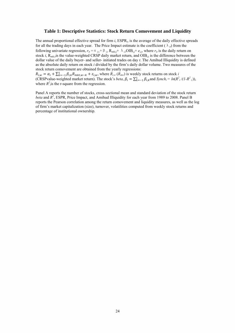
Table 1: Descriptive Statistics: Stock Return Comovement and Liquidity The annual proportional effective spread for firm i, ESPRi, is the average of the daily effective spreads for all the trading days in each year. The Price Impact estimate is the coefficient (λit) from the following univariate regression, rit =αi,t,+βi,t Rmkt,j+ λi,tOIBi,j+ ei,j, where rit is the daily return on stock i, Rmkt,tis the value-weighted CRSP daily market return, and OIBi,t is the difference between the dollar value of the daily buyer- and seller- initiated trades on day t. The Amihud Illiquidity is defined as the absolute daily return on stock i divided by the firm’s daily dollar volume. Two measures of the stock return comovement are obtained from the yearly regressions:

, ∑ , , , , where Ri,w (Rmw) is weekly stock returns on stock i (CRSPvalue-weighted market return). The stock’s beta, ∑ , and Synchi = ln(R2

i /(1-R2 i,)),

where R2iis the r-square from the regression.

Panel A reports the number of stocks, cross-sectional mean and standard deviation of the stock return beta and R2, ESPR, Price Impact, and Amihud Illiquidity for each year from 1989 to 2008. Panel B reports the Pearson correlation among the return comovement and liquidity measures, as well as the log of firm’s market capitalization (size), turnover, volatilities computed from weekly stock returns and percentage of institutional ownership.

25

Panel A: Summary Statistics

Year Sample

Size Statistics R2 Beta ESPR(%)

Price Impact

Amihud Illiquidity

1989 1115 Mean 0.234 1.064 79.831 2.83 15.58

Std. Deviation 0.151 0.870 66.484 9.15 47.58

1990 1072 Mean 0.281 1.103 92.279 2.81 23.54

Std. Deviation 0.169 0.722 77.363 8.24 63.13

1991 1086 Mean 0.276 1.249 89.225 2.67 19.68

Std. Deviation 0.137 0.841 71.368 8.23 61.68

1992 1214 Mean 0.146 1.091 84.522 2.72 16.44

Std. Deviation 0.104 1.214 68.730 8.15 53.41

1993 1347 Mean 0.149 1.177 80.930 2.73 13.12

Std. Deviation 0.101 1.392 68.350 8.61 46.25

1994 1445 Mean 0.171 1.146 80.340 2.33 12.58

Std. Deviation 0.106 0.899 66.457 6.78 40.45

1995 1485 Mean 0.128 0.981 77.488 2.30 11.12

Std. Deviation 0.094 1.426 66.633 7.28 38.97

1996 1516 Mean 0.193 0.879 70.369 1.80 8.85

Std. Deviation 0.127 0.812 62.577 5.39 30.95

1997 1579 Mean 0.182 0.856 57.007 1.50 6.33

Std. Deviation 0.125 0.652 51.063 4.16 22.68

1998 1591 Mean 0.292 1.219 56.459 1.67 7.66

Std. Deviation 0.152 0.808 51.237 5.33 26.14

1999 1533 Mean 0.113 0.718 62.407 2.16 8.57

Std. Deviation 0.106 0.794 55.821 6.43 29.42

2000 1424 Mean 0.107 0.511 68.517 2.53 12.78

Std. Deviation 0.090 0.894 67.289 6.99 45.36

2001 1297 Mean 0.175 0.660 40.126 1.84 9.95

Std. Deviation 0.138 0.770 45.064 5.89 40.48

2002 1284 Mean 0.377 0.908 29.693 1.53 9.26

Std. Deviation 0.193 0.696 37.743 4.89 41.03

2003 1310 Mean 0.291 1.030 20.209 1.15 5.42

Std. Deviation 0.165 0.833 25.721 4.39 27.69

2004 1303 Mean 0.270 1.167 15.784 0.72 3.83

Std. Deviation 0.128 0.822 22.510 3.29 23.05

2005 1322 Mean 0.236 1.183 13.706 0.57 3.82

Std. Deviation 0.127 0.926 20.097 3.55 31.19

2006 1325 Mean 0.237 1.277 11.674 0.44 2.64

Std. Deviation 0.132 1.150 15.661 2.42 21.68

2007 1308 Mean 0.287 1.121 9.755 0.19 2.05

Std. Deviation 0.140 0.836 10.365 0.80 18.65

2008 1297 Mean 0.390 1.412 20.460 0.58 8.61

Std. Deviation 0.165 0.872 25.413 3.14 100.81

1989~2008 Overall Average 0.223 1.029 52.786 1.73 9.78

26

Panel B: Correlations

R-square Beta ESPR%Price

Impact Amihud

Illiquidity Total

VolatilityIdiosyncratic

Volatility Size Turnover

Institutional Ownership

R-square 1.00 0.36 -0.35 -0.20 -0.19 -0.12 -0.30 0.39 0.07 0.19 Beta 1.00 0.06 -0.02 -0.05 0.47 0.37 -0.05 0.33 0.11

ESPR% 1.00 0.65 0.59 0.48 0.53 -0.67 -0.14 -0.36 Price Impact 1.00 0.63 0.25 0.28 -0.41 -0.15 -0.26

Amihud Illiquidity 1.00 0.15 0.19 -0.38 -0.18 -0.26 Total Volatility 1.00 0.98 -0.37 0.46 -0.04

Idiosyncratic Volatility 1.00 -0.42 0.42 -0.07 Size 1.00 0.07 0.27

Turnover 1.00 0.35 Institutional Ownership 1.00

27

Table 2: Liquidity and Return Comovement: Cross-sectional Tests

We regress stock liquidity measures on stock return synchronicity (Synch), Beta, total volatility (TotVol), idiosyncratic volatility (IdioVol), systematic volatility (SysVol), and other control variables, using yearly observations of individual firms, using fixed-effect panel regression method. Synch is the logit-transformation of R2 from the market-model regression for each stock. Beta is the beta coefficient in the market-model regression.TotVolis the standard deviation of a stock’s weekly returns.IdioVolrepresents the standard deviation of the weekly residual returns from the market model. SysVolis measured by square root of the explained variation of the market-model regression. A total of four control variables are included. Size is the log value of the firm’s capitalization measured at the beginning of the year. IOis the percentage institutional ownership measured at the beginning of the year. Turnover is the daily number of shares traded divided by total shares outstanding in the year. If the dependent variable is the proportional effective spread, we also include the inverse of the price level (1/P) of the stock at the beginning of the year. The three firm-level liquidity measures are the proportional effective spreads, price impact, and Amihud illiquidity. The regression results based on the three liquidity measures are reported in Panels A, B, and C respectively. In each panel we provide the regression results based on the full sample period (1989 to 2008), and two sub-periods, 1989-1998, and 1999-2008. The firm and year clustered t-statistics are reported in the parenthesis.

28

Table 2: Liquidity and Return Comovement: Cross-sectional Tests (cont’d)

Panel A: Dependent Variable = Effective proportional bid-ask spread

Synch Beta IdioVol SysVol Size IO Turnover 1/P

Sample Period:

1989~2008

-3.25 -9.08 -18.02 -1.42 4.88(-4.84) (-12.02) (-7.58) (-0.80) (-7.05)

-2.42 3.97 -8.63 -17.39 -8.84 4.39 (-4.78) (4.38) (-12.87) (-6.53) (-2.20) (6.79)

4.64 -2.99 -8.35 -17.35 -7.98 4.38 (5.21) (-5.42) (-12.36) (-6.51) (-1.98) (6.78)

Sample Period:

1989~1998

-3.60 -9.53 -7.51 -12.95 7.75(-6.39) (-12.29) (-3.23) (-3.08) (19.76)

-2.30 7.54 -8.21 -6.02 -40.29 6.80 (-4.03) (7.82) (-11.89) (-2.60) (-5.55) (19.54)

8.07 -2.99 -7.93 -5.67 -39.51 6.81 (8.35) (-5.35) (-11.29) (-2.46) (-5.58) (19.45)

Sample Period:

1999~2008

-2.13 -7.60 -15.15 -2.80 2.64(-2.05) (-5.18) (-4.82) (-1.67) (5.09)

-2.14 2.98 -7.15 -13.90 -7.60 2.27 (-2.01) (4.36) (-5.31) (-4.32) (-2.61) (5.15)

3.48 -2.13 -6.95 -14.03 -7.10 2.25 (4.94) (-4.78) (-5.18) (-4.35) (-2.53) (5.10)

29

Table 2: Liquidity and Return Comovement: Cross-sectional Tests (cont’d)

Panel B: Dependent Variable = Price Impact

Synch Beta IdioVol SysVol Size IO Turnover

Sample Period:

1989~2008

-0.36 -1.29 -3.67 -0.46 (-3.38) (-9.36) (-8.48) (-1.98)

-0.41 0.48 -1.12 -3.30 -1.32 (-6.10) (4.18) (-9.99) (-7.76) (-2.61)

-0.53 -0.32 -1.08 -3.35 -1.27 (4.82) (-4.35) (-9.55) (-7.60) (-2.38)

Sample Period:

1989~1998

-0.29 -1.71 -4.06 -2.18 (-2.23) (-10.70) (-8.19) (-3.46)

-0.48 1.05 -1.23 -3.02 -5.92 (-5.28) (7.28) (-10.83) (-7.15) (-5.27)

1.03 -0.25 -1.22 -3.12 -6.04 (8.27) (-2.01) (-10.86) (-7.48) (-5.09)

Sample Period:

1999~2008

-0.31 -0.92 -2.73 -0.38 (-2.02) (-5.38) (-4.86) (-2.07)

-0.25 0.26 -0.83 -2.51 -0.78 (-2.25) (3.36) (-5.49) (-4.50) (-2.45)

0.32 -0.26 -0.81 -2.53 -0.71 (4.03) (-3.57) (-5.21) (-4.48) (-2.23)

30

Table 2: Liquidity and Return Comovement: Cross-sectional Tests (cont’d)

Panel C: Dependent Variable = Amihud illiquidity

Synch Beta IdioVol SysVol Size IO Turnover

Sample Period: 1989~2008

-2.73 -7.81 -21.72 -6.79 (-3.18) (-9.16) (-5.53) (-4.02)

-2.93 2.42 -7.18 -20.12 -10.63 (-4.62) (5.37) (-9.02) (-5.35) (-4.48)

2.93 -2.75 -6.90 -20.21 -10.00 (4.75) (-3.81) (-8.75) (-5.35) (-4.18)

Sample Period: 1989~1998

-2.38 -10.08 -15.89 -22.05 (-2.06) (-7.92) (-4.32) (-3.90)

-2.84 4.35 -8.38 -12.05 -36.90 (-4.35) (4.76) (-7.89) (-3.65) (-4.21)

4.68 -2.59 -8.19 -12.09 -36.76 (4.83) (-2.50) (-8.09) (-3.72) (-4.20)

Sample Period: 1999~2008

-2.59 -5.97 -22.29 -4.65 (-2.09) (-6.40) (-4.01) (-4.19)

-2.45 1.88 -5.53 -20.88 -7.22 (-2.35) (2.59) (-6.40) (-4.06) (-4.36)

2.45 -2.49 -5.25 -20.95 -6.59 (2.47) (-2.76) (-6.00) (-4.07) (-4.42)

31

Table 3: Changes in Liquidity and Return Comovement

We regress yearly changes of stock liquidity measures on yearly changes of stock return synchronicity (Synch), Beta, total volatility (TotVol), idiosyncratic volatility (IdioVol), systematic volatility (SysVol), and changes of other control variables, using the fixed-effect panel regression method. Synch is the logit-transformation of R2 from the market-model regression for each stock. Beta is the beta coefficient in the market-model regression.TotVolis the standard deviation of a stock’s weekly returns.IdioVolrepresents the standard deviation of the weekly residual returns from the market model. SysVolis measured by square root of the explained variation of the market-model regression. A total of four control variables are included. Size is the log value of the firm’s capitalization measured at the beginning of the year. IOis the percentage institutional ownership measured at the beginning of the year. Turnover is the daily number of shares traded divided by total shares outstanding in the year. If the dependent variable is the proportional effective spread, we also include the inverse of the price level (1/P) of the stock at the beginning of the year. The three firm-level liquidity measures are the proportional effective spreads (ESPR), price impact, and Amihud illiquidity (Amihud). The regression is based on the sample period from 1989 to 2008. The firm and year clustered t-statistics are reported in the parenthesis.

Dependent Variables

ΔSynch ΔBeta ΔIdioVol ΔSysVol ΔSize ΔIO ΔTurnover Δ1/P

ΔESPR

-2.39 -15.64 -12.55 -7.58 1.85 (-5.78) (-19.22) (-4.12) (-4.50) (4.02)

-0.72 4.57 -14.23 -13.01 -18.36 1.53 (-1.87) (8.10) (-19.57) (-4.18) (-5.72) (3.69)

4.95 -1.49 -13.95 -12.12 -17.43 1.53 (8.68) (-4.27) (-19.12) (-4.07) (-5.82) (3.72)

ΔPrice Impact

-0.11 -1.56 -0.16 -0.45 (-2.38) (-12.98) (-0.80) (-4.07)

-0.19 0.32 -1.36 -0.15 -1.20 (-2.76) (5.72) (-12.81) (-0.67) (-5.41)

0.32 -0.02 -1.36 -0.13 -1.21 (6.27) (-0.62) (-12.56) (-0.59) (-5.08)

ΔAmihud

-0.97 -10.53 -3.18 -3.06 (-2.46) (-10.36) (-1.08) (-4.19)

-1.27 2.36 -9.12 -3.15 -8.45 (-3.18) (4.02) (-8.98) (-1.10) (-4.50)

2.53 -0.90 -9.00 -2.58 -8.03 (3.57) (-1.50) (-8.36) (-0.95) (-4.75)

32

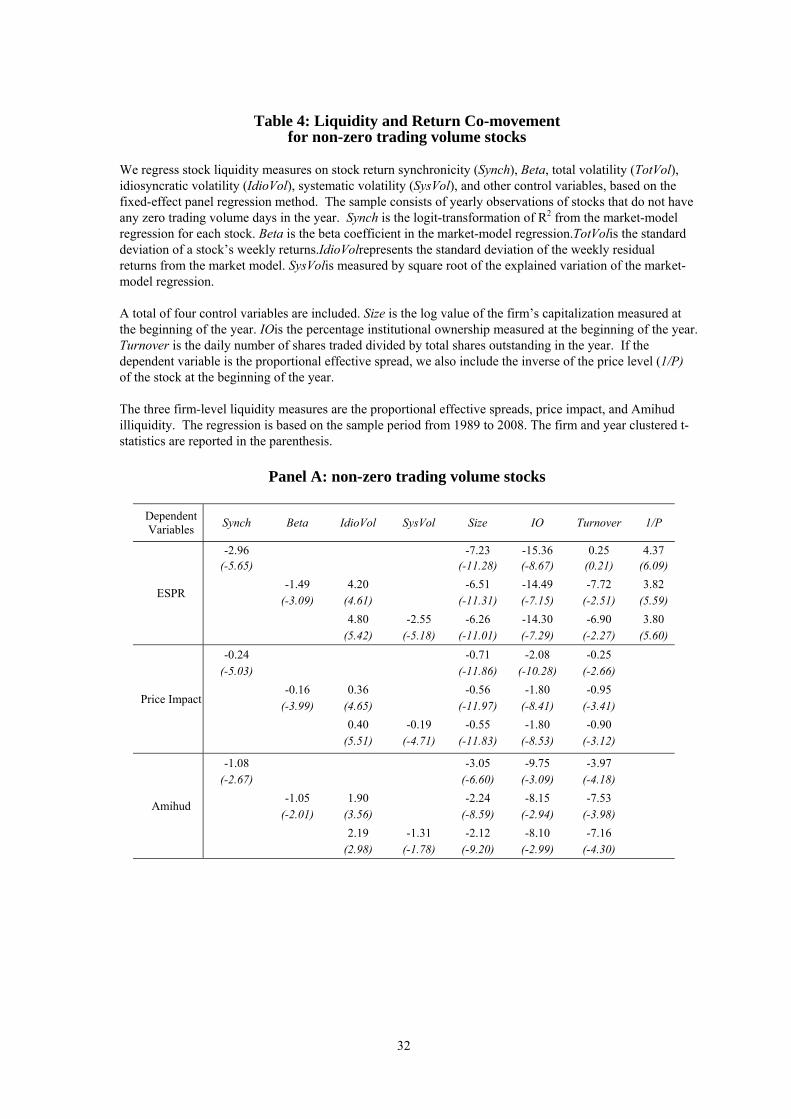
Table 4: Liquidity and Return Co-movement

for non-zero trading volume stocks We regress stock liquidity measures on stock return synchronicity (Synch), Beta, total volatility (TotVol), idiosyncratic volatility (IdioVol), systematic volatility (SysVol), and other control variables, based on the fixed-effect panel regression method. The sample consists of yearly observations of stocks that do not have any zero trading volume days in the year. Synch is the logit-transformation of R2 from the market-model regression for each stock. Beta is the beta coefficient in the market-model regression.TotVolis the standard deviation of a stock’s weekly returns.IdioVolrepresents the standard deviation of the weekly residual returns from the market model. SysVolis measured by square root of the explained variation of the market-model regression. A total of four control variables are included. Size is the log value of the firm’s capitalization measured at the beginning of the year. IOis the percentage institutional ownership measured at the beginning of the year. Turnover is the daily number of shares traded divided by total shares outstanding in the year. If the dependent variable is the proportional effective spread, we also include the inverse of the price level (1/P) of the stock at the beginning of the year. The three firm-level liquidity measures are the proportional effective spreads, price impact, and Amihud illiquidity. The regression is based on the sample period from 1989 to 2008. The firm and year clustered t-statistics are reported in the parenthesis.

Panel A: non-zero trading volume stocks

Dependent Variables

Synch Beta IdioVol SysVol Size IO Turnover 1/P

ESPR

-2.96 -7.23 -15.36 0.25 4.37(-5.65) (-11.28) (-8.67) (0.21) (6.09)

-1.49 4.20 -6.51 -14.49 -7.72 3.82 (-3.09) (4.61) (-11.31) (-7.15) (-2.51) (5.59)

4.80 -2.55 -6.26 -14.30 -6.90 3.80 (5.42) (-5.18) (-11.01) (-7.29) (-2.27) (5.60)

Price Impact

-0.24 -0.71 -2.08 -0.25 (-5.03) (-11.86) (-10.28) (-2.66)

-0.16 0.36 -0.56 -1.80 -0.95 (-3.99) (4.65) (-11.97) (-8.41) (-3.41)

0.40 -0.19 -0.55 -1.80 -0.90 (5.51) (-4.71) (-11.83) (-8.53) (-3.12)

Amihud

-1.08 -3.05 -9.75 -3.97 (-2.67) (-6.60) (-3.09) (-4.18)

-1.05 1.90 -2.24 -8.15 -7.53 (-2.01) (3.56) (-8.59) (-2.94) (-3.98)

2.19 -1.31 -2.12 -8.10 -7.16 (2.98) (-1.78) (-9.20) (-2.99) (-4.30)

33

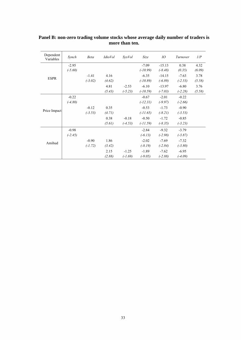
Panel B: non-zero trading volume stocks whose average daily number of traders is

more than ten.

Dependent Variables

Synch Beta IdioVol SysVol Size IO Turnover 1/P

ESPR

-2.95 -7.09 -15.13 0.38 4.32(-5.60) (-10.99) (-8.48) (0.35) (6.09)

-1.41 4.16 -6.35 -14.15 -7.63 3.78 (-3.02) (4.62) (-10.89) (-6.89) (-2.53) (5.58)

4.81 -2.53 -6.10 -13.97 -6.80 3.76 (5.43) (-5.23) (-10.59) (-7.03) (-2.28) (5.58)

Price Impact

-0.22 -0.67 -2.01 -0.22 (-4.80) (-12.31) (-9.97) (-2.66)

-0.12 0.35 -0.53 -1.73 -0.90 (-3.53) (4.71) (-11.65) (-8.21) (-3.53)

0.38 -0.18 -0.50 -1.72 -0.85 (5.61) (-4.53) (-11.59) (-8.35) (-3.23)

Amihud

-0.98 -2.84 -9.32 -3.79 (-2.45) (-6.13) (-2.98) (-3.87)

-0.90 1.86 -2.02 -7.69 -7.32 (-1.72) (3.42) (-8.19) (-2.84) (-3.80)

2.15 -1.25 -1.89 -7.62 -6.95 (2.88) (-1.69) (-9.05) (-2.88) (-4.09)

34

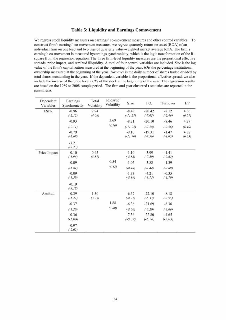
Table 5: Liquidity and Earnings Comovement

We regress stock liquidity measures on earnings’ co-movement measures and other control variables, To construct firm’s earnings’ co-movement measures, we regress quarterly return-on-asset (ROA) of an individual firm on one lead and two lags of quarterly value-weighted market average ROA. The firm’s earning’s co-movement is measured byearnings synchronicity, which is the logit-transformation of the R-square from the regression equation. The three firm-level liquidity measures are the proportional effective spreads, price impact, and Amihud illiquidity. A total of four control variables are included. Size is the log value of the firm’s capitalization measured at the beginning of the year. IOis the percentage institutional ownership measured at the beginning of the year. Turnover is the daily number of shares traded divided by total shares outstanding in the year. If the dependent variable is the proportional effective spread, we also include the inverse of the price level (1/P) of the stock at the beginning of the year. The regression results are based on the 1989 to 2008 sample period. The firm and year clustered t-statistics are reported in the parenthesis.

Dependent Variables

Earnings Synchronicity

Total Volatility

Idiosync Volatility Size I.O. Turnover 1/P

ESPR -0.96 2.94 -8.48 -20.42 -8.12 4.36 (-2.12) (4.08) (-11.27) (-7.63) (-2.46) (6.57)

-0.93 3.69 -8.21 -20.10 -8.46 4.27

(-2.11) (4.76) (-11.02) (-7.28) (-2.56) (6.40)

-0.79 -9.10 -19.31 -1.47 4.82

(-1.69) (-11.70) (-7.56) (-1.05) (6.83)

-3.21 (-3.23)

Price Impact -0.10 0.45 -1.10 -3.99 -1.41 (-1.96) (3.87) (-8.88) (-7.59) (-2.62)

-0.09 0.54 -1.05 -3.88 -1.39

(-1.84) (4.42) (-8.48) (-7.44) (-2.69)

-0.09 -1.33 -4.21 -0.35

(-1.59) (-8.89) (-8.15) (-1.70)

-0.19 (-3.18)

Amihud -0.39 1.50 -6.57 -22.10 -8.18 (-1.27) (3.25) (-8.71) (-6.33) (-2.95)

-0.37 1.88 -6.36 -21.69 -8.36

(-1.20) (3.80) (-8.60) (-6.20) (-3.06)

-0.36 -7.36 -22.80 -4.65

(-1.08) (-8.39) (-6.78) (-3.05)

-0.97 (-2.62)

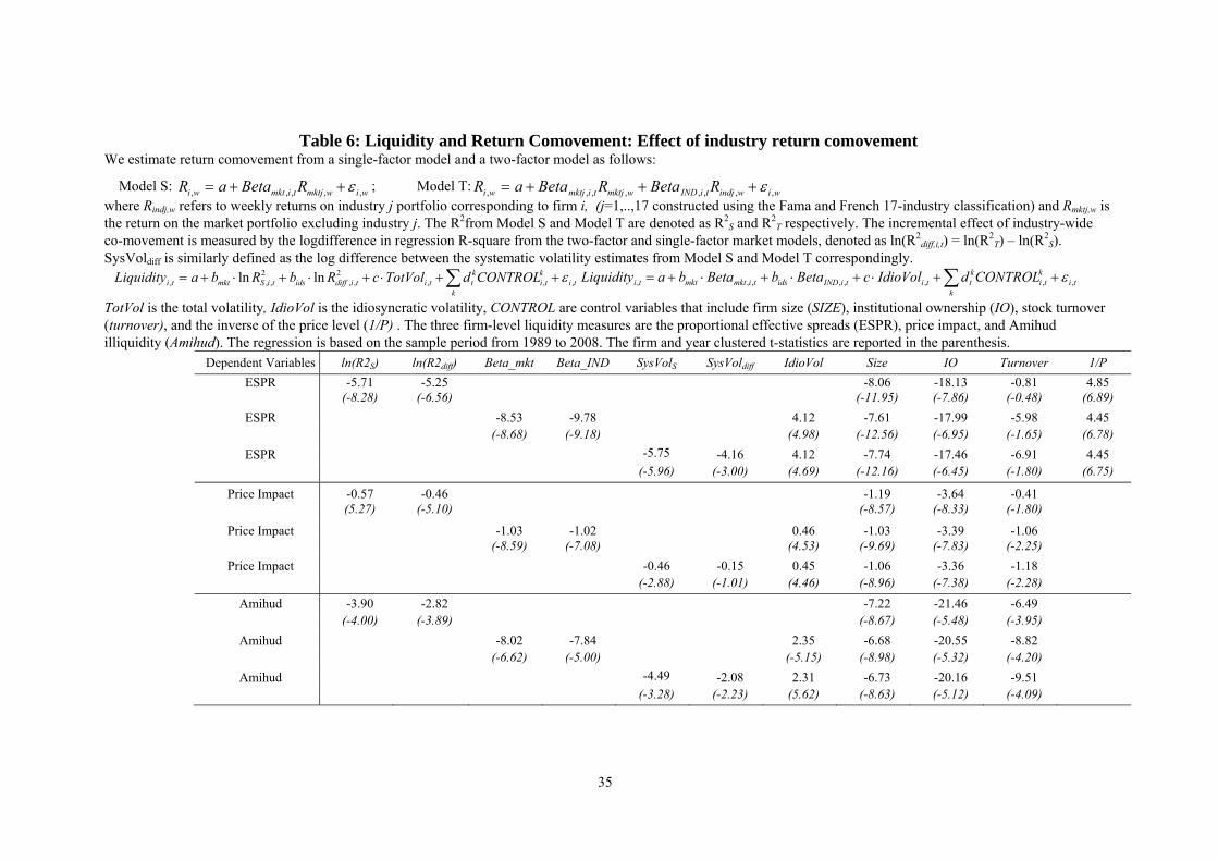
35

Table 6: Liquidity and Return Comovement: Effect of industry return comovement We estimate return comovement from a single-factor model and a two-factor model as follows:

Model S: wiwmktjtimktwi RBetaaR ,,,,, ; Model T: wiwindjtiINDwmktjtimktjwi RBetaRBetaaR ,,,,,,,, where Rindj,w refers to weekly returns on industry j portfolio corresponding to firm i, (j=1,..,17 constructed using the Fama and French 17-industry classification) and Rmktj,w is the return on the market portfolio excluding industry j. The R2from Model S and Model T are denoted as R2

S and R2T respectively. The incremental effect of industry-wide

co-movement is measured by the logdifference in regression R-square from the two-factor and single-factor market models, denoted as ln(R2diff,i,t) = ln(R2

T) – ln(R2S).

SysVoldiff is similarly defined as the log difference between the systematic volatility estimates from Model S and Model T correspondingly.

tik

kti

kttitidiffidstiSmktti CONTROLdTotVolcRbRbaLiquidity ,,,

2,,

2,,, lnln ti

k

kti

kttitiINDidstimktmktti CONTROLdIdioVolcBetabBetabaLiquidity ,,,,,,,,

TotVol is the total volatility, IdioVol is the idiosyncratic volatility, CONTROL are control variables that include firm size (SIZE), institutional ownership (IO), stock turnover (turnover), and the inverse of the price level (1/P) . The three firm-level liquidity measures are the proportional effective spreads (ESPR), price impact, and Amihud illiquidity (Amihud). The regression is based on the sample period from 1989 to 2008. The firm and year clustered t-statistics are reported in the parenthesis.

Dependent Variables ln(R2S) ln(R2diff) Beta_mkt Beta_IND SysVolS SysVoldiff IdioVol Size IO Turnover 1/P

ESPR -5.71 -5.25 -8.06 -18.13 -0.81 4.85 (-8.28) (-6.56) (-11.95) (-7.86) (-0.48) (6.89)

ESPR -8.53 -9.78 4.12 -7.61 -17.99 -5.98 4.45 (-8.68) (-9.18) (4.98) (-12.56) (-6.95) (-1.65) (6.78)

ESPR -5.75 -4.16 4.12 -7.74 -17.46 -6.91 4.45 (-5.96) (-3.00) (4.69) (-12.16) (-6.45) (-1.80) (6.75)

Price Impact -0.57 -0.46 -1.19 -3.64 -0.41 (5.27) (-5.10) (-8.57) (-8.33) (-1.80)

Price Impact -1.03 -1.02 0.46 -1.03 -3.39 -1.06 (-8.59) (-7.08) (4.53) (-9.69) (-7.83) (-2.25)

Price Impact -0.46 -0.15 0.45 -1.06 -3.36 -1.18 (-2.88) (-1.01) (4.46) (-8.96) (-7.38) (-2.28)

Amihud -3.90 -2.82 -7.22 -21.46 -6.49 (-4.00) (-3.89) (-8.67) (-5.48) (-3.95)

Amihud -8.02 -7.84 2.35 -6.68 -20.55 -8.82 (-6.62) (-5.00) (-5.15) (-8.98) (-5.32) (-4.20)

Amihud -4.49 -2.08 2.31 -6.73 -20.16 -9.51 (-3.28) (-2.23) (5.62) (-8.63) (-5.12) (-4.09)

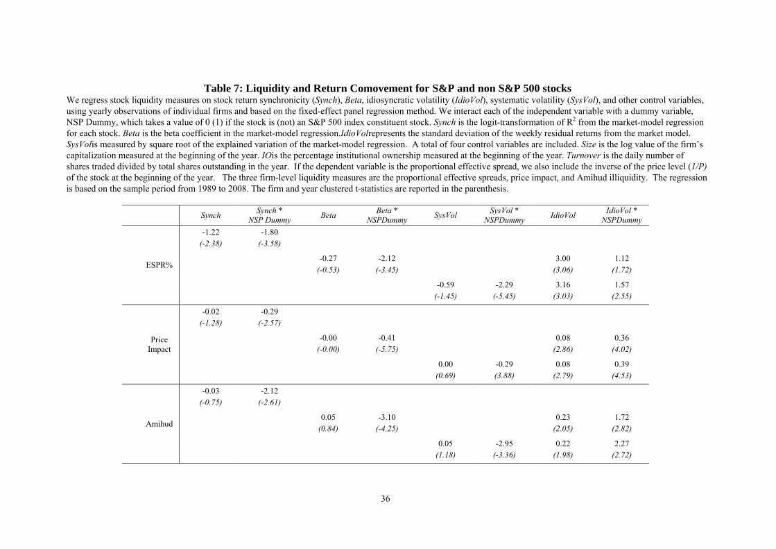
36

Table 7: Liquidity and Return Comovement for S&P and non S&P 500 stocks We regress stock liquidity measures on stock return synchronicity (Synch), Beta, idiosyncratic volatility (IdioVol), systematic volatility (SysVol), and other control variables, using yearly observations of individual firms and based on the fixed-effect panel regression method. We interact each of the independent variable with a dummy variable, NSP Dummy, which takes a value of 0 (1) if the stock is (not) an S&P 500 index constituent stock. Synch is the logit-transformation of R2 from the market-model regression for each stock. Beta is the beta coefficient in the market-model regression.IdioVolrepresents the standard deviation of the weekly residual returns from the market model. SysVolis measured by square root of the explained variation of the market-model regression. A total of four control variables are included. Size is the log value of the firm’s capitalization measured at the beginning of the year. IOis the percentage institutional ownership measured at the beginning of the year. Turnover is the daily number of shares traded divided by total shares outstanding in the year. If the dependent variable is the proportional effective spread, we also include the inverse of the price level (1/P) of the stock at the beginning of the year. The three firm-level liquidity measures are the proportional effective spreads, price impact, and Amihud illiquidity. The regression is based on the sample period from 1989 to 2008. The firm and year clustered t-statistics are reported in the parenthesis.

Synch Synch *

NSP DummyBeta

Beta * NSPDummy

SysVol SysVol *

NSPDummyIdioVol

IdioVol * NSPDummy

ESPR%

-1.22 -1.80 (-2.38) (-3.58)

-0.27 -2.12 3.00 1.12 (-0.53) (-3.45) (3.06) (1.72)

-0.59 -2.29 3.16 1.57 (-1.45) (-5.45) (3.03) (2.55)

Price Impact

-0.02 -0.29 (-1.28) (-2.57)

-0.00 -0.41 0.08 0.36 (-0.00) (-5.75) (2.86) (4.02)

0.00 -0.29 0.08 0.39 (0.69) (3.88) (2.79) (4.53)

Amihud

-0.03 -2.12 (-0.75) (-2.61)

0.05 -3.10 0.23 1.72 (0.84) (-4.25) (2.05) (2.82)

0.05 -2.95 0.22 2.27 (1.18) (-3.36) (1.98) (2.72)

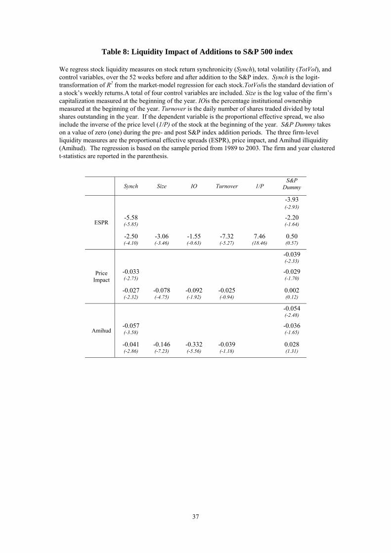
37

Table 8: Liquidity Impact of Additions to S&P 500 index

We regress stock liquidity measures on stock return synchronicity (Synch), total volatility (TotVol), and control variables, over the 52 weeks before and after addition to the S&P index. Synch is the logit-transformation of R2 from the market-model regression for each stock.TotVolis the standard deviation of a stock’s weekly returns.A total of four control variables are included. Size is the log value of the firm’s capitalization measured at the beginning of the year. IOis the percentage institutional ownership measured at the beginning of the year. Turnover is the daily number of shares traded divided by total shares outstanding in the year. If the dependent variable is the proportional effective spread, we also include the inverse of the price level (1/P) of the stock at the beginning of the year. S&P Dummy takes on a value of zero (one) during the pre- and post S&P index addition periods. The three firm-level liquidity measures are the proportional effective spreads (ESPR), price impact, and Amihud illiquidity (Amihud). The regression is based on the sample period from 1989 to 2003. The firm and year clustered t-statistics are reported in the parenthesis.

Synch Size IO Turnover 1/P S&P

Dummy

ESPR

-3.93 (-2.93)

-5.58 -2.20 (-5.85) (-1.64)

-2.50 -3.06 -1.55 -7.32 7.46 0.50 (-4.10) (-3.46) (-0.63) (-5.27) (18.46) (0.57)

Price Impact

-0.039 (-2.33)

-0.033 -0.029 (-2.75) (-1.70)

-0.027 -0.078 -0.092 -0.025 0.002 (-2.32) (-4.75) (-1.92) (-0.94) (0.12)

Amihud

-0.054 (-2.48)

-0.057 -0.036 (-3.58) (-1.65)

-0.041 -0.146 -0.332 -0.039 0.028 (-2.86) (-7.23) (-5.56) (-1.18) (1.31)