K.7

Stock Market Cross-Sectional Skewness and Business Cycle Fluctuations Ferreira, Thiago R.T.

International Finance Discussion Papers Board of Governors of the Federal Reserve System

Number 1223 March 2018

Please cite paper as: Ferreira, Thiago R.T. (2018). Stock Market Cross-Sectional Skewness and Business Cycle Fluctuations. International Finance Discussion Papers 1223. https://doi.org/10.17016/IFDP.2018.1223

Board of Governors of the Federal Reserve System

International Finance Discussion Papers

Number 1223

March 2018

Stock Market Cross-Sectional Skewness and Business Cycle Fluctuations

Thiago R.T. Ferreira NOTE: International Finance Discussion Papers are preliminary materials circulated to stimulate discussion and critical comment. References to International Finance Discussion Papers (other than an acknowledgment that the writer has had access to unpublished material) should be cleared with the author or authors. Recent IFDPs are available on the Web at www.federalreserve.gov/pubs/ifdp/. This paper can be downloaded without charge from the Social Science Research Network electronic library at www.ssrn.com.

Stock Market Cross-Sectional Skewness

and Business Cycle Fluctuations∗

Thiago R. T. Ferreira†

Federal Reserve Board

Abstract

Using U.S. data from 1926 to 2015, I show that financial skewness—a measure comparing

cross-sectional upside and downside risks of the distribution of stock market returns of

financial firms—is a powerful predictor of business cycle fluctuations. I then show that

shocks to financial skewness are important drivers of business cycles, identifying these

shocks using both vector autoregressions and a dynamic stochastic general equilibrium

model. Financial skewness appears to reflect the exposure of financial firms to the

economic performance of their borrowers.

Key Words: Cross-Sectional Skewness, Business Cycle Fluctuations, Financial Channel.

JEL Classification: C32, E32, E37, E44.

∗This version: February 2018. First version: June 2017. This paper was previously circulated as “Cross-Section Skewness, Business Cycle Fluctuations and the Financial Accelerator Channel.”†Division of International Finance, Federal Reserve Board, 20th and C St. NW, Washington, DC 20551.

Email: thiago.r.teixeiraferreira@frb.gov. Phone: (202) 973-6945. The views expressed in this paper are solelymy responsibility and should not be interpreted as reflecting the views of the Board of Governors of the FederalReserve System or of any other person associated with the Federal Reserve System. I am very thankful for theoutstanding research assistance of George Jiranek. I am very grateful for the discussions with Andrea Raffo. Iam also indebted to Rob Vigfusson, Matteo Iaconviello, and Larry Christiano for comments and suggestions.I am also grateful for the discussions at the Board of Governors, Banque de France, Federal Reserve Bankof Philadelphia, 2017 Workshop on Time-Varying Uncertainty in Macro (University of Saint Andrews), 2017Southern Economic Association Meeting, and 2018 AEA meetings.

1

1 Introduction

Historically, economists have been engaged in both predicting and understanding the origins

of business cycle fluctuations. Recently, much of this literature has analyzed how fluctuations

in uncertainty about economic variables affect business cycles.1 However, the focus on uncer-

tainty overlooks the role of tail risks, as both downside and upside risks increase uncertainty

while generally leading to divergent economic outcomes. Moreover, there is still little evidence

on how the interplay between these tail risks contribute to the prediction and explanation of

business cycles. In this paper, I show evidence that a measure of cross-sectional skewness—

i.e., the balance between cross-sectional upside and downside risks—not only has a powerful

predictive ability on economic activity, but also seems to be an important source of cyclical

fluctuations for the US economy.

Figure 1: Cross-Sectional Distribution of Stock Market Returns of Financial Firms

(a) Probability Density Function

Log returns (percent)-60 -40 -20 0 20 40 60

0

2

4

6

8

10

2006:Q22008:Q4

Downside Risks Upside Risks( ) ( )

(b) Cross-Sectional Moments

2006:Q2 2008Q4Median 0% 0%Dispersion 20% 86%Skewness 0% -27%

I demean the cross-sectional distributions of stock market returns and then I calculate skewness by[(r95t − r50

t )− (r50t − r5

t )],

dispersion by (r95t − r5

t ), upside risks by (r95t − r50

t ), and downside risks by (r50t − r5

t ), where rpt is the pth percentile of thedistribution of log-returns at time t.

I define financial skewness as a measure comparing cross-sectional upside and down-

side risks of the distribution of log-returns of financial firms. Specifically, I calculate it by

[(r95t −r50

t )−(r50t −r5

t )], where rpt is the pth percentile of the distribution of log-returns at time t,

(r95t −r50

t ) measures upside risks, and (r50t −r5

t ) measures downside risks. Thus, if financial skew-

ness is negative, the balance of cross-sectional risks is tilted to the downside, while if financial

skewness is positive, risks are tilted to the upside. Figure 1 shows the distribution of log-

returns of financial firms for 2006:Q2 and 2008:Q4. It documents that financial skewness

1See Bloom (2014) for a literature review on this topic.

2

became markedly negative from 2006:Q2 to 2008:Q4, as the increase in downside risks was

substantially larger than the increase in upside risks.

The relationship between financial skewness and the business cycle appears to be robust

across time as well as quantitatively powerful. First, I document that financial skewness closely

tracks business cycles over the period 1926 to 2015 (Figure 2), with correlations higher than

those associated with most other variables. Second, I present evidence showing that financial

skewness has a strong predictive power on several measures of economic activity. Using

in-sample and out-of-sample regressions for the 1973 to 2015 sample, I show that financial

skewness generally performs better than many well-known indicators of economic conditions,

such as bond spreads (e.g., Gilchrist and Zakrajsek (2012)), measures of aggregate uncertainty

(e.g., Jurado et al. (2015), and Ludvigson et al. (2015)) and other moments from the cross-

sectional distribution of returns. Finally, I show that these results are not dependent on specific

events, such as the Great Recession, as financial skewness performs well in both recessions

and expansions.

Figure 2: Financial Skewness and the Business Cycle

-23

-14

-5

4

13

Q1-1927

Q2-1933

Q4-1939

Q1-1946

Q2-1952

Q3-1958

Q4-1964

Q2-1971

Q3-1977

Q4-1983

Q1-1990

Q3-1996

Q4-2002

Q1-2009

Q2-2015-4

0

4

9

13Percent Percent

GDP Growth(Right)

FinancialSkewness(Left)

Figure 2 shows the 4-quarter moving average of financial skewness in blue and the 4-quarter GDP growth in red. Grayareas represent periods classified as recessions by the NBER.

I argue that this tight relationship between financial skewness and the business cycle re-

flects the exposure of financial firms to the economic performance of their borrowers. This

hypothesis is based on three arguments. First, financial firms focus on specific loan markets

they expect to boost their equity returns. Second, stock markets evaluate these exposures of

financial firms to specific markets by pricing higher equity valuations for those firms financing

borrowers with higher expected profits. Then, as economic shocks (e.g. technology innova-

tions and policy surprises) impact different nonfinancial firms differently, the cross-section of

stock returns of financial firms signals how the distribution of profitability of their borrowers

3

reacts to these shocks. Third, because financial firms also diversify idiosyncratic risks across

loan markets, financial firms’ stock returns signal risks related to investment projects most

impactful to the macroeconomy.

I provide three pieces of empirical evidence to support this hypothesis that financial skew-

ness signals the economic performance of their borrowers. First, I show that cross-sectional

distributions of stock market returns of financial firms have less dispersion and thinner tails

than those of nonfinancial firms. This result is consistent with financial firms being exposed

to specifically chosen loan markets while achieving some diversification across markets. Sec-

ond, I show that variables associated with asset quality of financial firms, such as banks’

asset returns, account for 76% of the fluctuations in financial skewness. Moreover, since these

variables are released after the end of the quarter, results indicate that financial skewness

anticipates financial firms’ asset quality. Third, I document that financial skewness also leads

credit market conditions, such as loan growth. This last result points to stock markets timely

pricing credit market fundamentals, especially for a submarket for which financial firms are

expected to have a comparative advantage in sorting borrower quality.

I then investigate the quantitative role of shocks to financial skewness in explaining busi-

ness cycles. For this, I use two complementary approaches: a dynamic stochastic general

equilibrium (DSGE) model and Bayesian vector autoregressions (BVARs). The DSGE model

rationalizes the hypothesis that financial firms are exposed to specific loan markets, embeds a

financial accelerator channel, and allows cross-sectional risks to be subject to skewness shocks,

thus modeling heterogeneous effects of macroeconomic shocks. The BVARs have more flexible

identifications of skewness shocks and their transmission channels. Both the DSGE model and

BVARs estimate that financial skewness shocks are important business cycle drivers, have siz-

able economic effects, and account for most of the fluctuations in financial skewness, displacing

many other shocks studied in the literature including cross-sectional dispersion ones.2

Finally, I provide evidence that an important transmission channel of financial skewness

shocks is consistent with models of financial frictions. I support this argument with three

results. First, both the DSGE model and BVARs estimate that when cross-sectional risks are

exogenously tilted to the downside, nonfinancial firms receive less credit, face higher lending

interest rates, have lower equity values, invest less, and produce less. Second, I document

that the effects on economic activity from skewness shocks are amplified when lending rates

respond more to these shocks.3 Third, I show that the response of many macroeconomic

2Bachmann and Bayer (2014) and Zeke (2016) use calibrated theoretical models to provide different argu-ments on why dispersion shocks should not be viewed as important business cycle drivers.

3See Caldara et al. (2016) for related evidence using uncertainty measures focused on second moments,such as dispersion and volatility.

4

variables to skewness shocks in the BVARs are consistent with analogous responses from the

DSGE model with financial frictions used in this paper.

Differently from most of the literature studying the sources of business cycle fluctuations,

this paper argues that cross-sectional tail risks are important drivers of these fluctuations. In

one branch of this literature, many business cycle theories advocate that idiosyncratic risk—

i.e., the cross-sectional idiosyncratic component of firms’ behavior—is an important driver of

aggregate fluctuations.4 However, these papers overlook the aggregate effects from shocks to

cross-sectional upside and downside risks, with most them focusing on dispersion shocks. In

another branch of this literature, many papers analyze the relationship between tail risks and

the macroeconomy, although they focus on aggregate tail risks.5 This paper shows evidence

that cross-sectional skewness—i.e. the balance between upside and downside cross-sectional

risks—is an important source of aggregate fluctuations.6

Lastly, this paper has several contributions to the literature studying the predictive ability

of financial indicators on economic conditions. First, it shows that financial skewness is a

powerful predictor of economic activity, performing better than many influential financial

indicators cited in the literature.7 Second, this paper provides evidence that stock markets

can be an effective barometer of economic fundamentals. This argument is supported by the

predictive ability of financial skewness on economic activity and by the data corroborating

the interpretation that financial skewness reflects the economic health of its borrowers. This

argument also challenges the hypothesis that bond markets are more accurate than stock

markets about economic fundamentals.8 Third, this paper provides evidence of a measure of

cross-sectional idiosyncratic risk that performs well in both predicting and driving economic

fluctuations. Despite the importance of idiosyncratic risk in business cycle theories, empirical

measures of it have had little influence on the research seeking to predict these same aggregate

fluctuations.

4These papers argue that shocks to idiosyncratic risk have economic effects through several channels: wait-and-see effects from capital adjustment frictions (Bloom et al. (2012)); financial frictions (Arellano et al.(2012), Christiano et al. (2014), Gilchrist et al. (2014), and Chugh (2016)); search frictions in the labormarket (Schaal (2017)); agency problems in the management of the firm (Panousi and Papanikolaou (2012));granular effects (Gabaix (2011)); and network effects (Acemoglu et al. (2012)).

5For instance, see Barro (2006), Gabaix (2012), and Gorio (2012).6Kelly and Jiang (2014) show some evidence on the relationship between cross-sectional downside risks

economic activity, although the focus of their analysis is on asset pricing. Other papers document thathigh-order moments of the cross-sectional distribution of many economic variables seem to co-move with theeconomic cycle, such as firm sales, profit, and employment (Bloom et al. (2016)); household income (Guvenenet al. (2014)); and price changes (Luo and Vallenas (2017)).

7For literature reviews on this topic, see Stock and Watson (2003) and Ng and Wright (2013).8See Philippon (2009), Gilchrist and Zakrajsek (2012), and Lopez-Salido et al. (2017) for different versions

of this argument.

5

2 Financial Skewness and Business Cycles

In this section, I describe the cross-sectional distribution measures used in this paper (Section

2.1), and document that financial skewness stands out not only as a close tracker of business

cycles (Section 2.2), but also as a powerful predictor of economic activity (Section 2.3).

2.1 Cross-Sectional Distribution Measures

I use U.S. stock market returns from the CRSP database for the period from 1926:Q1 to

2015:Q2. I define Ri,st as the stock market gross return of firm i at sector s and quarter

t, ri,st = log(Ri,st ) as the log-return of firm i at quarter t, and rp,st as the pth percentile of

the distribution of log-returns within sector s at quarter t. Then, I calculate sectoral cross-

sectional measures of mean, dispersion, skewness, left kurtosis, and right kurtosis as follows:

mean: M(1)st = 100Ns,t

(∑i∈sR

i,st − 1

), for s ∈ {fin, nfin}, (1)

dispersion: M(2)st = r95,st − r5,s

t , for s ∈ {fin, nfin}, (2)

skewness: M(3)st = (r95,st − r50,s

t )− (r50,st − r5,s

t ), for s ∈ {fin, nfin}, (3)

left kurtosis: M(4)st = (r45,st − r25,s

t )− (r25,st − r5,s

t ), for s ∈ {fin, nfin}, (4)

right kurtosis: M(5)st = (r95,st − r75,s

t )− (r75,st − r55,s

t ), for s ∈ {fin, nfin}, (5)

where Ns,t is the number of firms in sector s at quarter t and “fin” and “nfin” represent

financial and nonfinancial sectors of the U.S. economy, respectively.9 Notice that the intuition

for left kurtosis (equation (4)) and right kurtosis (equation (5)) is analogous to the one for

skewness, with the difference being that these kurtoses measures compare upside and downside

risks within each distribution tail using the 25th and 75th quartiles as their reference returns.

I also calculate cross-sectional distribution measures weighted by firm size. To do so, for

each time t, sector s, and return Ri,st , I artificially augment the sample by repeating return

Ri,st proportionally to its market capitalization share in its sector s at quarter t. Then, I

apply the same formulas (1)-(5). Throughout this paper, unless otherwise noted, I refer to

unweighted measures. Thus, I refer to unweighted M(3)fint as financial skewness, unweighted

M(3)nfint as nonfinancial skewness, and analogously for other distribution measures.10

9The classification between financial and nonfinancial sectors is according to the NAICS codes. WhenNAICS codes are not available, I use SIC codes. For details, see Appendix A.1.

10I use raw realized returns to calculate measures (1)-(5), instead of residuals of regressions on marketfactors, such as Fama-French (1993). I choose this procedure because market returns themselves may bedetermined by the distribution of idiosyncratic risks (e.g., Ferreira (2016)). Thus, if the goal is to measureaggregate effects from time-varying idiosyncratic risk, one may be excluding important information throughthese factor regressions. Alternatively, I control for aggregate factors, such as market returns and volatility,by including direct measures of them in the regressions of this paper.

6

2.2 Financial Skewness Tracks Business Cycles

Table 1 documents the correlations between financial and nonfinancial skewness and measures

of economic activity for the period 1926–2015. Two results emerge. First, correlations are

higher for financial skewness relative to the nonfinancial skewness, regardless of the activity

measure and sample period. Second, correlations are higher for the 1985–2015 period relative

to the full sample, regardless of the activity and skewness measures. Notably, the correlation

between financial skewness and GDP growth in the 1985–2015 period is 0.71.

Table 1: Correlations between Cross-Sectional Skewness and the Business Cycle

Expansion Indicator GDP Growth

SampleFinancial Nonfinancial Financial NonfinancialSkewness Skewness Skewness Skewness

1926∗–2015 0.34 0.31 0.40 0.361986–2015 0.59 0.49 0.71 0.42

I use 4-quarter moving averages of unweighted skewness, 4-quarter GDP growth, and an expansion indicator from the NBERclassification. ∗For GDP growth, the larger sample ranges from 1947 to 2015.

I then measure the co-movement between all distribution measures (1)-(5) and the business

cycle by estimating logit regressions on the NBER expansion indicator. This dependent

variable not only encompasses a wide set of information about the economic cycle, but also is

available for the whole sample period for which the distribution measures are calculated: 1926

to 2015. Thus, we can interpret the results from these logit regressions as being robust to

specific historical periods, such as the Great Depression, the Great Moderation, and the Great

Recession. As control variables, I include the spread between Moody’s Baa and Aaa corporate

rates (Baa-Aaa spread) and the lagged NBER expansion indicator. Finally, I standardize the

series of all regressors to ensure comparability between the estimated coefficients. Table 2

displays regression estimates.

These logit regressions show that financial skewness is one of the variables most correlated

with the business cycle and that this correlation is quantitatively relevant. These conclusions

come from four results. First, financial skewness adds more explanatory power (pseudo R2)

to the benchmark regression with only lagged NBER-indicator than most other variables

(columns (1)-(7) of Tables 2a-2b). Second, the correlation of financial skewness and the

cycle is robust to the inclusion of other variables, with its coefficient retaining an intuitive

sign and being statistically significant (regressions (8)-(9) of Table 2a). Third, within the

universe of the largest specifications (columns (9)-(10) of Tables 2a-2b), the coefficient of

financial skewness is the second largest, only lower than the one associated with the weighted

nonfinancial mean. Finally, declines in financial skewness imply considerable increases in

recession probabilities. For instance, when the economy is expanding, a drop of two standard

7

Table 2: Logit Regressions on NBER Expansion Indicator, 1926–2015

(a) Financial Distribution Measures

Regressions with Unweighted Distribution Measures WeightedVariables (1) (2) (3) (4) (5) (6) (7) (8) (9) (10)

Constant -1.26*** -1.55*** -1.11*** -1.36*** -1.24*** -1.35*** -1.22*** -1.73*** -1.77*** -1.77***Expansion lag 4.12 4.55 3.93 4.38 4.11 4.23 4.04 5.02 5.05 4.95Mean 1.17*** 1.33*** 1.23** 1.50***Dispersion -0.34 -0.44 -0.68 -0.47Skewness 1.17*** 1.71** 1.68** 0.90*Left kurtosis 0.43 -0.92* -0.98* -0.42Right kurtosis 0.20 -0.69 -0.64 -0.79Baa-Aaa -0.24** 0.23 0.10Pseudo R2 0.53 0.58 0.54 0.57 0.54 0.53 0.55 0.62 0.63 0.62

(b) Nonfinancial Distribution Measures

Regressions with Unweighted Distribution Measures WeightedVariables (1) (2) (3) (4) (5) (6) (7) (8) (9) (10)

Constant -1.26*** -1.55*** -1.24*** -1.27*** -1.29*** -1.25*** -1.22*** -1.54*** -1.54*** -1.75***Expansion lag 4.12 4.58 4.09 4.37 4.20 4.24 4.04 4.76 4.78 4.99Mean 1.30*** 1.05** 1.17* 1.85***Dispersion -0.09 -1.03 -0.84 -1.57**Skewness 1.06*** -0.43 -0.47 -0.13Left kurtosis 0.40 0.15 0.30 -1.27Right kurtosis 0.79** 1.44 1.38 0.62Baa-Aaa -0.24** -0.13 -0.02Pseudo R2 0.53 0.59 0.53 0.57 0.54 0.55 0.55 0.61 0.61 0.62

Distribution measures are included in the regression as they are calculated in equations (1)-(5). All regressors are standardized,except the lagged expansion indicator. I include two lags of the expansion indicator because it has a lower AIC score. For allother regressors, I include its contemporaneous and one lagged values. The coefficients reported are the sum of all coefficientsassociated with a particular regressor. Statistical significance tests the null hypothesis that all coefficients associated to aregressor equal to zero, where ∗, ∗∗, and ∗ ∗ ∗ denote significance levels of 0.1, 0.05, and 0.01.

deviations in financial skewness sustained over the previous and current quarters implies a

52% probability of recession in the current quarter.11

2.3 Financial Skewness is a Powerful Predictor of Business Cycles

The following features are common to all regressions in this section: (i) I restrict the sample

to the period 1973:Q1-2015:Q2, as some of the best-performing competing variables are not

available before this period; (ii) I standardize all regressors, thus enabling the comparison

between regression coefficients; and (iii) for a variable Yt, I forecast Yt+h|t−1 at time t, where

Yt+h|t−1 =

400h+1 ln

(Yt+hYt−1

), if Yt is nonstationary,

Yt+h, if Yt is stationary.

11For this computation, I use the estimates of specification (9) and assume that (i) financial skewness equalsto minus 2, (ii) expansion lag is 1, and (iii) all remaining regressors are at their historical mean values.

8

Thus, for instance, I forecast the mean annualized real GDP growth h quarters ahead, while

I forecast the level of the unemployment rate h quarters ahead. Finally, I consider several

competing variables to financial skewness. Besides financial and nonfinancial distribution

measures (1)-(5), I use (i) financial uncertainty (Ludvigson et al. (2016)), proxying for ag-

gregate uncertainty from financial markets; (ii) GZ-spread (Gilchrist and Zakrajsek (2012)),

representing the large literature on corporate credit spreads; (iii) term spread, measured by

the difference between the 10-year Treasury constant maturity and the three-month Treasury

bill rates; and (iv) the real fed funds rates, measuring the current monetary policy stance.

For short, I refer to variables (i)-(iv) as economic predictors.

2.3.1 In-Sample Predictive Regressions on Economic Activity

In this section, the general form of the in-sample regressions is

Yt+h|t−1︸ ︷︷ ︸economic activity measure

= α+

p∑i=1

ρiYt−i|t−i−1︸ ︷︷ ︸lagged forecasted variable

+5∑

k=1

q∑j=0

βkjM(k)t−j︸ ︷︷ ︸distribution measures

+

q∑j=0

γjzt−j︸ ︷︷ ︸economic predictors

+et+h. (6)

I focus on predictions for four quarters ahead (h = 4). Also, I make p = 4 because of the

relatively high Akaike information criterion (AIC) of this specification and q = 1 to keep

the model parsimonious. I calculate the elasticities of regressor variables by summing the

coefficients of each regressor’s contemporaneous and lagged values. Thus, if a regressor Xt

has an elasticity of C% on dependent variable Yt+h|t−1, a decrease of one standard deviation

in Xt lasting periods t and t− 1 should decrease Yt+h|t−1 by C%. Lastly, I compute standard

errors using Hodrick (1992).

Table 3 reports the results of regression (6) on GDP growth, with financial skewness having

a large explanatory power as well as a high elasticity on GDP growth. Table 3 focuses on

unweighted distribution measures, with Table 3a showing the results of distribution measures

of the financial firms’ returns.12 In Table 3a, column (1) represents the benchmark model

only with lags of GDP growth (βkj = γj = 0, ∀j, k), while columns (2)-(10) represent models

adding one variable at a time to the benchmark model. Comparing these 10 regressions, we

see that financial skewness not only improves the benchmark’s in-sample fit (R2) by one of the

largest amounts—20 percentage points—but also has the largest elasticity on GDP growth: a

decline of one standard deviation of financial skewness lasting two consecutive quarters leads

to a drop of 1.2% in the mean GDP growth over the next four quarters.

12Results for weighted measures are shown in Table 12 of Appendix A.3, with weighted financial skewnessperforming only slightly worse than nonweighted financial skewness.

9

Table 3: In-Sample GDP Forecast Regressions, Four Quarters Ahead, 1973–2015

(a) Financial Firms, Unweighted Distribution Measures

Regressions SpecificationsVariable (1) (2) (3) (4) (5) (6) (7) (8) (9) (10) (11) (12)

Mean 1.19*** 0.73*Dispersion -0.15* 1.07**Skewness 1.20*** 1.60** 1.00***Left kurtosis 0.71** 0.26Right kurtosis 0.46** -1.06***Uncertainty -0.46** 0.24Real fed funds -0.44 0.18Term spread 0.92*** 1.03***GZ spread -0.55** -0.49R2 0.080.29 0.11 0.28 0.17 0.11 0.19 0.12 0.28 0.23 0.40 0.54

(b) Nonfinancial Firms, Unweighted Distribution Measures

Regressions SpecificationsVariable (1) (2) (3) (4) (5) (6) (7) (8) (9) (10) (11) (12)

Mean 1.11*** 1.40*** 0.57**Dispersion -0.15 0.01Skewness 0.61*** -1.98**Left kurtosis 0.38*** 1.16Right kurtosis 0.43*** 1.02Uncertainty -0.46** 0.10Real fed funds -0.44 0.06Term spread 0.92*** 0.96***GZ spread -0.55** -0.67R2 0.080.24 0.09 0.15 0.13 0.12 0.19 0.12 0.28 0.23 0.26 0.47

This table reports the results from regressions (6) on average GDP growth four quarters ahead (h = 4), with p equal to 4because of the relatively low AIC of this specification, and q equal to 1 to keep the model parsimonious. Real fed funds ismeasured by the fed funds rate minus the four-quarter change of core inflation from the personal consumption expenditures.The elasticities of regressor variables reported above are calculated by summing the contemporaneous and lagged coefficients

of each regressor,{βk =

∑qj=0 β

kj

}5

k=1and γ =

∑qj=0 γj. Coefficients of lagged GDP growth are omitted. Standard errors

are calculated according to Hodrick (1992). Statistical significance tests the null hypothesis that all coefficients associated toa regressor equal to zero, where ∗, ∗∗, and ∗ ∗ ∗ denote significance levels of 0.1, 0.05, and 0.01.

I then show that the predictive ability of financial skewness is robust to the inclusion

of other regressors. To avoid having an excessively large number of regressors, I proceed in

two steps. First, I include all financial distribution measures in one regression (column (11)

in Table 3a). The results show that financial skewness is statistically significant and has the

highest elasticity on GDP growth, 1.6%. Then, I include financial skewness in a regression with

all economic predictors (column (12) in Table 3a). Financial skewness remains statistically

significant and has one of the largest elasticities, 1%—a number somewhat smaller than the

ones from regressions (4) and (11).

Financial skewness also explains future GDP growth better than nonfinancial distribution

measures. Regressions (2)-(6) of Table 3b add one nonfinancial distribution measure at a

10

time to the benchmark model, regression (1). The R2s and elasticities from these regressions

are lower than those from the analogous regression with financial skewness (regression (4)

of Table 3a). Turning to the regressions with all nonfinancial measures (column (11)) and

all economic predictors (column (12)), even the nonfinancial measure with the largest and

intuitive elasticities—the mean—has these elasticities being lower that those associated with

financial skewness in analogous regressions (columns (11)-(12) of Table 3b relative to column

(11)-(12) of Table 3a).

Table 3 shows that the economic predictors’ regression estimates are broadly consistent

with results from other papers. In regressions (7)-(10), the coefficients of most variables are

statistically significant and with expected signs. For instance, a lower GDP growth is preceded

by higher financial uncertainty, lower term-spreads, and higher corporate spreads. However,

the coefficients of many of these variables, such as financial uncertainty and GZ-spread, either

lose their statistical significance or have unintuitive signs in the larger specifications (12)

of Tables 3a-3b. The only economic predictor with statistical significance in these larger

regressions is term-spread. Moreover, the magnitude of the elasticity of term-spread is similar

to the one of financial skewness.

Studying additional measures of economic activity, we learn that the predictive ability of

financial skewness goes beyond GDP growth. Table 4 reports the results for the following

variables: GDP, personal consumption expenditures, private fixed investment, total hours

worked, and unemployment rate. Table 4b focuses on the results of regressions that use finan-

cial skewness as a predictor variable. Row (a) shows estimates from benchmark regressions

only with lagged predicted variables, while rows (b) and (c) show the results for regressions

that add financial skewness to the benchmark. These first three rows document that financial

skewness adds about 10% to 25% of explanation power to future economic activity and has

statistically and economically significant elasticities, such as 3.9% on investment. Rows (d)

through (i) present the results of regressions adding both financial skewness and economic

predictors to benchmark regressions. In all of these regressions, financial skewness remains

statistically significant and has one of the largest elasticities, with these elasticities being of

sizable magnitudes.

Finally, financial skewness also performs better than other distribution measures across

many activity indicators. Given the large literature on dispersion measures, I focus on re-

sults comparing dispersion and skewness measures. Table 4b shows the results of financial

skewness, Table 4c of financial dispersion, Table 4e of nonfinancial skewness, and Table 4f of

nonfinancial dispersion. By comparing these tables, we first notice that financial skewness is

the distribution measure that adds the most explanatory power to predicted variables (row

11

Table 4: In-Sample Forecast Regressions, Macro Variables, Four Quarters Ahead, 1973–2015

(a) Notation

(a) Benchmark R2

(b)Bivariate

Variable(c) R2

(d)

Multivariate

Variable(e) Uncertainty(f) Real fed funds(g) Term spread(h) GZ spread(i) R2

(b) Variable = Financial Skewness

GDP Consumption Investment Hours U-rate

0.08 0.22 0.21 0.17 0.54

1.20*** 0.64*** 3.89*** 1.67*** -0.75***

0.28 0.31 0.39 0.41 0.67

1.00*** 0.71*** 2.72*** 0.89** -0.59***0.24 0.26 0.50 -0.13 0.070.18 0.36** -0.83 -0.45 0.151.03*** 0.84*** 2.76*** 0.87*** -0.36***

-0.49 -0.25 -1.86 -0.94** 0.12**

0.54 0.54 0.67 0.70 0.77

(c) Variable = Financial Dispersion

GDP Consumption Investment Hours U-rate

0.08 0.22 0.21 0.17 0.54

-0.15* 0.13** -0.77*** -0.72*** 0.51***

0.11 0.25 0.26 0.26 0.62

-0.29 -0.18 -0.91 -0.35 0.43**0.23 0.25 0.53 -0.12 -0.03**0.07 0.25 -1.14 -0.52 0.141.04*** 0.83*** 2.83*** 0.89*** -0.46***

-0.84** -0.48* -2.81** -1.28** 0.34***

0.46 0.48 0.61 0.66 0.75

(d) Notation

(a) Benchmark R2

(b)Bivariate

Variable(c) R2

(d)

Multivariate

Variable(e) Uncertainty(f) Real fed funds(g) Term spread(h) GZ spread(i) R2

(e) Variable = Nonfinancial Skewness

GDP Consumption Investment Hours U-rate

0.08 0.22 0.21 0.17 0.54

0.61*** 0.21*** 2.11*** 1.08*** -0.35***

0.15 0.25 0.28 0.28 0.57

0.21 0.07** 0.79 0.38 -0.170.06 0.16 0.07 -0.31 0.17**0.02 0.21 -1.22 -0.54 0.240.98*** 0.78*** 2.68*** 0.86*** -0.39***

-0.74 -0.46 -2.42 -1.09* 0.29**

0.45 0.48 0.61 0.66 0.72

(f) Variable = Nonfinancial Dispersion

GDP Consumption Investment Hours U-rate

0.08 0.22 0.21 0.17 0.54

-0.15 0.06 -0.62 -0.81*** -0.07

0.09 0.23 0.23 0.25 0.54

0.60** 0.47 1.90*** 0.31** -0.43***-0.06 0.05 -0.37 -0.36 0.27*-0.21 0.06 -2.01* -0.72 0.400.88*** 0.74*** 2.33*** 0.76*** -0.21*

-1.21*** -0.80** -3.99*** -1.44*** 0.56***

0.49 0.50 0.65 0.67 0.74

This table reports the results from regressions (6) on GDP, personal consumption expenditures, private fixed investment, total hours worked, and unemployment rate. With theexception of the unemployment rate, all predicted variables are used in growth rates, where h = 4, p = 4 because of the relatively low AIC of this specification, and q = 1 to keep themodel parsimonious. Real fed funds is measured by the fed funds rate minus the four-quarter change of core inflation from the personal consumption expenditures. The elasticities

of regressor variables reported above are calculated by summing the contemporaneous and lagged coefficients of each regressor,{βk =

∑qj=0 β

kj

}5

k=1and γ =

∑qj=0 γj. Coefficients

of lagged predicted variables are omitted. Standard errors are calculated according to Hodrick (1992). Statistical significance tests the null hypothesis that all coefficients associatedto a regressor equal to zero, where ∗, ∗∗, and ∗ ∗ ∗ denote significance levels of 0.1, 0.05, and 0.01.

12

(c) of all tables). Then, we see that financial skewness also has the largest elasticities, both

among the bivariate regressions (row (b) of all tables) and among the multivariate regressions

(row (d) of all tables). In short, results from this section point to a powerful predictive ability

of financial skewness on a broad range of measures of economic activity.

2.3.2 Out-of-Sample Predictive Regressions on GDP Growth

I then turn to a more stringent evaluation of the predictive ability of financial skewness by

calculating out-of-sample forecasts of GDP growth. To focus on the performance of predictor

variable Xt, I only include lags of GDP growth as additional regressors:

GDPXtt+h|t−1 = α +

p∑i=1

ρiGDPt−i|t−i−1 +

q∑j=0

θjXt−j + ut+h. (7)

The details of the forecasts and their performance evaluation are as follows. I extend the list

of predictor variables Xt beyond the ones in Section 2.3.1 by including Moody’s Baa corporate

yields minus 10-year Treasury yields (Baa-10y), Moody’s Baa yields minus Moody’s Aaa yields

(Baa-Aaa), and macroeconomic uncertainty (Jurado et al. (2016)). I also use forecasts from

regression (7) that only include lags of GDP growth (θj = 0, ∀j), referring to these forecasts

as GDP-AR. I determine the number of lags of GDP growth (p) and predictor variable Xt

(q) by choosing the specification with the minimum AIC at each forecasting period. I use an

expanding window of data with jump-off date 1986:Q1. I also add Consensus predictions to

the list of forecasts to evaluate predictions from regressions (7) against forecasts that use a

potentially wider information set.13 Finally, I document the performance of different variables

by computing ratios of root mean squared forecast errors (RMSFEs). I use financial skewness

as the benchmark variable and refer to these ratios as relative root mean squared forecast

error (R-RMSFE) of variable Xt. Values below 1 indicate that financial skewness performs

better than variable Xt.

Figure 3 shows the R-RMSFEs from these forecasts, with financial skewness outperforming

almost all variables. Figures 3a-3c focus on a set of selected predictor variables, providing

R-RMSFEs for the full sample, recessions, and expansions. On the full sample (Figure 3a),

R-RMSFEs are below 1 and statistically significant (estimates with circles) for almost all

variables and horizons (h = 2, 4, 6).14 Moreover, the magnitudes by which financial skewness

13Given that Consensus forecasts are released on the 10th of every month, I average forecasts from the lastmonth of the quarter with those from the month right after the end of quarter. For performance evaluation,I compare the times series of Consensus forecasts directly against realized GDP growth data.

14To calculate statistical significance, I use the Diebold-Mariano test (Diebold and Mariano (1995)) onthe difference between the RMSFE of the predictor variable and the RMSFE of financial skewness. I com-

13

Figure 3: Out-of-Sample Forecasts of GDP Growth, R-RMSFEs

(a) Full Sample

R-RMSFE in decimals0.6 0.7 0.8 0.9 1 1.1 1.2 1.3

Consensus

GDP-AR

Macro uncertainty

Baa-Aaa spread

Financial uncertainty

GZ spread

Baa-10y spread

Term spreadh=2

h=4

h=6

pval<0.1

pval<0.1

pval<0.1

(b) Recessions2

R-RMSFE in decimals

0.6 0.7 0.8 0.9 1 1.1 1.2 1.3

(c) Expansions3

R-RMSFE in decimals

0.6 0.7 0.8 0.9 1 1.1 1.2 1.3

(d) Nonweighted Measures

R-RMSFE in decimals

0.6 0.7 0.8 0.9 1 1.1 1.2 1.3Right kurtosis

Left kurtosis

Nonfinancial Skewness

Dispersion

Mean

—————————————-

Right kurtosis

Left kurtosis

Financial Skewness

Dispersion

Mean

(e) Weighted Measures

R-RMSFE in decimals

0.6 0.7 0.8 0.9 1 1.1 1.2 1.3

Figure 3 reports the ratio between the root mean squared forecast error (RMSFE) of financial skewness relative to theRMSFE of competing variables. I denote this ratio as relative root mean squared forecast error (R-RMSFE) and report itin decimals. Statistical significance is relative to the null hypothesis that the predictor variable and financial skewness haveequal predictive power. Circles represent significance levels of at least 10 percent. 2Recession R-RMSFEs are computed usingforecast errors from forecasts estimated during a quarter classified by the NBER as a recession. 3Expansion R-RMSFEs areanalogous to recession R-RMSFEs.

outperforms other variables range from 8% to 32% of improvement. R-RMSFEs from expan-

sions and recessions for selected variables (Figures 3b and 3c) yield results broadly similar to

those from the full sample, with statistical significance slightly more frequent in expansions.

Finally, Figures 3d and 3e show that financial skewness also outperforms almost all of the re-

pute this heteroskedasticity-autocorrelation (HAC) robust test by using the result from Kiefer and Vogelsang(2002). These authors show that using Bartlett kernel HAC standard errors without truncation yields the testdistribution from Kiefer et al. (2000). Abadir and Paruolo (2002) provide critical values for this distribution.

14

Figure 4: Forecasts of GDP Growth Four Quarters Ahead, Rolling 20-Quarter R-RMSFEs

(a) R-RMSFE of Macro Uncertainty

0

0.5

1

1.5

2

2.5

3

3.5

Q4-1990

Q3-1993

Q1-1996

Q4-1998

Q2-2001

Q4-2003

Q3-2006

Q1-2009

Q4-2011

Q2-2014

R-RMSFE in decimals

(b) R-RMSFE of Term-Spread

0

0.5

1

1.5

2

2.5

3

3.5

Q4-1990

Q3-1993

Q1-1996

Q4-1998

Q2-2001

Q4-2003

Q3-2006

Q1-2009

Q4-2011

Q2-2014

R-RMSFE in decimals

(c) R-RMSFE of GZ-Spread

0

0.5

1

1.5

2

2.5

3

3.5

Q4-1990

Q3-1993

Q1-1996

Q4-1998

Q2-2001

Q4-2003

Q3-2006

Q1-2009

Q4-2011

Q2-2014

R-RMSFE in decimals

(d) R-RMSFE of Consensus

0

0.5

1

1.5

2

2.5

3

3.5

Q4-1990

Q3-1993

Q1-1996

Q4-1998

Q2-2001

Q4-2003

Q3-2006

Q1-2009

Q4-2011

Q2-2014

R-RMSFE in decimals

Figure 4 reports the ratio between the root mean squared forecast error (RMSFE) of financial skewness relative to the RMSFEof competing variables. I denote this ratio as relative root mean squared forecast error (R-RMSFE) of variable Xt. At everyquarter, I compute the R-RMSFE over the current and past 19 quarters. Rolling 20-quarter R-RMSFEs are reported in decimals.

maining distribution variables, either weighted or unweighted.

For the few variables for which the performance comparison with financial skewness is

less straightforward, results still support the powerful predictive ability of financial skewness.

For instance, financial skewness performs as well as Consensus in the full sample and for

the forecast horizons available (h = 2, 4). Results are similar for expansions. In contrast,

Consensus statistically outperforms financial skewness in recessions, especially for predictions

for two quarters ahead. These results document that forecasts of financial skewness are most

often comparable with those using a wide information set, even though forecasts of financial

15

skewness come from a very simple model. The few other variables that outperform financial

skewness do not achieve statistical significance (e.g., weighted financial skewness) and/or are

statistically outperformed in one state of the cycle (e.g., macro uncertainty and GDP-AR).

Finally, I show that financial skewness has powerful predictive ability within the majority

of the sample period. Figure 4 displays 20-quarter rolling R-RMSFEs for GDP growth four

quarters ahead (h = 4), focusing on some well-known predictor variables: macro uncertainty

(Figure 4a), term spread (Figure 4b), GZ spread (Figure 4c), and Consensus (Figure 4d). For

most of the sample, Figures 4a-4c show that the rolling R-RMSFE stays below 1, indicating

that the forecasts using financial skewness have a lower RMSFE than those from alternative

variables. Although Figures 4a-4c point to some short-lived spikes to values higher than 1,

these figures show that financial skewness performs better than the competing variables in

many periods other than the Great Recession. Finally, Figure 4d shows financial skewness

and Consensus alternating in outperforming each other, with financial skewness generally

performing better in the first half of the sample.

3 Interpreting the Relationship between Financial

Skewness and the Business Cycle

In this section, I provide evidence supporting the hypothesis that the tight relationship be-

tween financial skewness and the business cycle originates from the exposure of financial firms

to the economic performance of their borrowers.

3.1 Financial Sector Diversifies Cross-Sectional Risks

The hypothesis above relies on the argument that financial firms focus on specific loan markets

they expect to boost their equity returns, while diversifying idiosyncratic risks across markets.

In turn, this partial diversification allows financial firms’ stock returns to signal risks related

to investment projects most impactful to the macroeconomy. I support this argument by

showing that cross-sectional distributions of stock market returns of financial firms are less

dispersed than those of nonfinancial firms, as well as less concentrated in the tails.

Table 5 reports time series averages of moments of cross-sectional distributions of stock

market returns. Specifically, it reports these averages for returns of financial and nonfinancial

firms during the periods 1926-2015 and 1947-2015. We see that in both sample periods returns

are less dispersed (row (b), columns (3) and (6)) and less concentrated in the tails (rows (d)-

(e), columns (3) and (6)) for financial firms relative to nonfinancial ones, while mean returns

16

Table 5: Time Series Averages of Distribution Measures (in percent)

Sample 1926 - 2015 Sample 1947 - 2015Financial Nonfinancial Difference Financial Nonfinancial Difference

(1) (2) (3) = (1) - (2) (4) (5) (6) = (4) - (5)(a) Mean 3.3 3.7 -0.5 2.9 3.4 -0.5(b) Dispersion 36.5 49.2 -12.7*** 35.8 58.8 -23.0***(c) Skewness -0.4 -0.1 -0.3 -1.1 -2.0 0.9*(d) Left Kurtosis -7.1 -9.0 1.9*** -7.9 -12.1 4.3***(e) Right Kurtosis 7.2 9.1 -1.9*** 7.0 11.0 -4.0***

Time series averages reported in Table 5 are computed from unweighted distribution measures. Statistical significance teststhe null hypothesis that cross-sectional moments are the same for returns from financial and nonfinancial firms, where *, **,and *** denote significance levels of 0.1, 0.05 and 0.01. Results are similar if computed for weighted distribution measures.

across financial firms are not statistically different from those across nonfinancial firms (row

(a), columns (3) and (6)).

In Figures 5a and 5b, I illustrate how this partial diversification of risks allows financial

skewness to better signal economic activity relative to its nonfinancial counterpart. These

figures show the evolution of GDP growth and financial and nonfinancial skewness in the

past three recessions. While financial skewness follows GDP growth very closely (Figure 5a),

nonfinancial skewness is noisier and has peaks and troughs disproportional to the cyclical

variation of GDP around the early 2000s recession (Figure 5b).15

Figure 5: Cross-Sectional Skewness and Last Three Recessions

(a) Financial Skewness

-23

-15

-7

0

8

Q1-1989

Q1-1992

Q4-1994

Q4-1997

Q4-2000

Q3-2003

Q3-2006

Q3-2009

Q2-2012

Q2-2015-4

-2

1

3

5

Financial Skewness

GDP Growth

Percent Percent

(b) Nonfinancial Skewness

-22

-11

-0

10

21

Q1-1989

Q1-1992

Q4-1994

Q4-1997

Q4-2000

Q3-2003

Q3-2006

Q3-2009

Q2-2012

Q2-2015-4

-2

1

3

5

Nonfinancial Skewness

GDP Growth

Percent Percent

Figures 5a and 5b show 4-quarter GDP growth and 4-quarter moving average of financial skewness (dark blue) and nonfinancialskewness (light blue). Gray areas represent periods classified as recessions by the NBER.

15These large increases and decreases in nonfinancial skewness around the early 2000s are present not onlyin the nonweighted nonfinancial skewness, but also in its weighted version and in the nonfinancial skewnessmeasures calculated by Bloom et al. (2016).

17

One criticism about the results above is that they rely on the distribution of equity returns,

while the hypothesis of the paper could be interpreted as more closely related to asset returns.

However, combining results from Table 5 with the fact that financial firms are generally more

leveraged than nonfinancial ones tells us that asset returns should also be less dispersed across

financial firms relative to nonfinancial ones.

3.2 Financial Skewness Signals Financial Firms’ Asset Quality

I then argue that financial skewness captures stock markets’ views about the quality of fi-

nancial firms’ assets. If this hypothesis is correct, variables measuring the quality of financial

firms’ assets should then account for a considerable amount of the variation in financial skew-

ness. Indeed, I show that 76% of the evolution of financial skewness in a recent sample

is accounted for by two variables: return on average assets for banks (ROA) and changes

in banks’ lending standards.16 Moreover, these two variables are released between one and

one and a half months after the end of the quarter, indicating that financial skewness also

anticipates information contained in these two variables.

Figure 6 and Table 6 describe the key results from this section. Figures 6a and 6b display

the series of ROA and changes in banks’ lending standards to small firms (LSSF), respectively.

These figures show a moderate amount of co-movement between these variables and the four-

quarter moving average of financial skewness. Table 6a then measures these co-movements

with simple univariate regressions. It shows that ROA explain 64% of the variation in financial

skewness, while LSSF explains 41%. Changes in lending standards to medium and large firms

(LSMLF) explain 34% of financial skewness, somewhat less than LSSF and consistent with

financial firms providing more information about nonfinancial firms with less access to capital

markets. Finally, the first column of Table 6b shows that a regression with ROA and LSSF

explains 76% of the variation in financial skewness. This result is also shown in Figure 6c,

where the fitted values of this last regression are plotted against financial skewness.

One concern about the results above is that ROA and LSSF may explain a large share of the

variation in financial skewness mostly because they co-move with aggregate macroeconomic

and financial conditions. To shed light on this issue, I add the following variables in the

regressions on financial skewness: the Chicago Fed’s Adjusted Financial Condition Index

(AFCI), excess bond premium (EBP), VIX and Consensus forecasts for GDP growth for the

16More precisely, the variable is the net percentage of domestic banks tightening standards for commercialand industrial loans. The interpretation of banks’ lending standards as being informative about financial firms’assets is based on the results of Basset et al. (2014). After accounting for endogenous responses to aggregatemacro and financial conditions, the authors argue that changes in banks’ lending standards reflect issues suchas reassessments of the riskiness of certain loans and changes in business strategies.

18

Figure 6: Financial Skewness and Banks’ Asset Quality

(a) Banks’ Return on Assets

-23

-15

-7

0

8

Q1-1989

Q1-1992

Q4-1994

Q4-1997

Q4-2000

Q3-2003

Q3-2006

Q3-2009

Q2-2012

Q2-2015-0.1

0.3

0.7

1.1

1.5

Financial Skewness

Return on Assets

Percent Percent

(b) Changes in Lending Standards for Small Firms

-23

-15

-7

0

8

Q1-1989

Q1-1992

Q4-1994

Q4-1997

Q4-2000

Q3-2003

Q3-2006

Q3-2009

Q2-2012

Q2-2015-75

-50

-25

-0

25

Financial Skewness

(Minus) Lending Standards

Percent Percent

(c) Fitted Values from Banks’ Return on Assets and Change in Lending Standards for Small Firms

-25

-20

-15

-10

-5

0

5

10

Q1-1989

Q1-1992

Q4-1994

Q4-1997

Q4-2000

Q3-2003

Q3-2006

Q3-2009

Q2-2012

Q2-2015

Financial Skewness

Fitted Values

Percent

All figures show the 4-quarter moving average of financial skewness in blue. Figure 6a plots in red the return on average assetsfor banks (ROA). Figure 6b plots in green the negative of the changes in banks’ lending standards to small firms (LSSF). Figure6c plots in black the fitted values of a regression using only the contemporaneous values of ROA and LSSF on the 4-quarteraverage of financial skewness.

current quarter and for the next four quarters ahead.17 Table 6b provides the estimates, with

all coefficients reflecting the fact that regressors are standardized within the sample. These

estimates show that variables proxying macro and financial conditions add little explanatory

power to a regression using ROA and LSSF. Moreover, Table 6b also shows that the coefficients

of these macro and financial indicators are smaller than those from ROA and LSSF. Although

17Chicago Fed’s Adjusted Financial Condition Index (AFCI) uses a large set of financial variables whilepurging out the influence of business cycle conditions (Brave and Butters (2011)). Excess bond premium(EBP) reflects liquidity risks and shifts in risk bearing capacity by financial firms (Gilchrist and Zakrajek(2012)) and credit market sentiment associated with credit booms and busts (Lopez-Salido et al. (2017)).VIX reflects not only uncertainty about the stock market, but also risk appetite (Bekaert et al. (2013)).

19

Table 6: Regressions on Financial Skewness

(a) Univariate Regressions

ROA LSSF LSLMF AFCI EBP VIXTerm

GDPConsensust|t−1 GDPConsensus

t+4|t−1Spread4.6*** -3.6*** -3.3*** -3.8*** -3.4*** -3.5*** -0.4 3.8*** 3.6***

R2 0.64 0.41 0.34 0.44 0.36 0.39 0.01 0.44 0.41

(b) Multivariate Regressions

Variable: AFCI EBP VIXTerm

GDPConsensust|t−1 GDPConsensus

t+4|t−1SpreadROA 3.7*** 3.5*** 3.6*** 3.5*** 4.0*** 3.4*** 3.5***LSSF -2.1*** -1.6*** -1.6*** -1.4*** -1.9*** -1.8*** -1.9***Variable -0.8* -0.7* -1.3*** 0.6** 0.8** 0.4R2 0.76 0.76 0.76 0.79 0.76 0.77 0.76

Regressions described in Tables 6a and 6b share the following features: sample period 1990Q1-2015Q2, standardized regressorswithin this sample, and 4-quarter moving average of financial skewness as the dependent variable. Table 6a describes theresults from univariate regressions using contemporaneous column variables. The first column of Table 6b displays the resultsof a regression using contemporaneous values of ROA and LSSF. The remaining columns of Table 6b use as regressors thecontemporaneous values of ROA, LSSF and the column variable. Statistical significance tests the null hypothesis that thecoefficient associated to a regressor is zero, where *, **, and *** denote significance levels of 0.1, 0.05 and 0.01.

these results are consistent with macro and financial conditions accounting for some variation

in financial skewness, they point to ROA and LSSF as being more prominent drivers.

3.3 Financial Skewness Anticipates Credit Market Conditions

Finally, if financial skewness anticipates economic activity because it signals the quality of

projects being financed by the financial sector, it should then also anticipate future credit

market conditions. Indeed, financial skewness not only leads several credit variables, but it

also performs particularly well in explaining future loan growth, a market in which financial

firms are expected to have comparative advantage in sorting borrower quality.

The empirical strategy of this section is similar to the one used in Section 2.3.1. I use

regression specifications (6) with the following dependent variables at four quarters ahead

(h=4): loan growth, debt growth, loan spread, GZ spread, and Baa-10y spread. I report

results in Table 7 not only for financial skewness, but also for nonfinancial dispersion, given

the relevance of the latter in the literature of time-varying uncertainty.18 Row (a) reports

estimates from benchmark regressions using only lagged predicted variables as regressors.

Rows (b) and (c) report estimates from regressions with a distribution measure added to the

benchmark regressions. Finally, rows (d) through (i) report estimates from regressions with a

18I report results for financial dispersion and nonfinancial skewness in Table 13 of Appendix A.3. The resultsfor these measures have less clear patterns than those reported here.

20

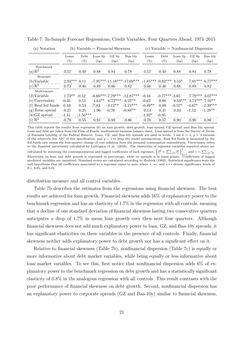
Table 7: In-Sample Forecast Regressions, Credit Variables, Four Quarters Ahead, 1973–2015

(a) Notation

Benchmark

(a)R2

Bivariate

(b)Variable(c) R2

Multivariate

(d)Variable(e) Uncertainty(f) Real fed funds(g)Term spread(h)GZ spread(i) R2

(b) Variable = Financial Skewness

Loans Debt Loan Sp GZ Sp Baa-10y

(%) (%) (bp) (bp) (bp)

0.57 0.40 0.88 0.84 0.78

2.93*** 0.11 -7.95***-11.18***-17.69***0.73 0.40 0.89 0.86 0.82

1.73** -0.52 -6.66***-7.79*** -12.87***-0.35 0.51 4.64** 6.72*** 6.27**-0.59 0.53 -7.83 -4.12** -3.15***0.21 0.25 1.96 -0.76 -0.88**

-1.41 -1.56***0.79 0.55 0.91 0.88 0.86

(c) Variable = Nonfinancial Dispersion

Loans Debt Loan Sp GZ Sp Baa-10y

(%) (%) (bp) (bp) (bp)

0.57 0.40 0.88 0.84 0.78

-1.85*** -0.82*** 3.53* 7.01*** 6.77***0.66 0.46 0.88 0.89 0.82

-0.16 -0.77***-3.65 7.79*** 3.07***-0.62 0.80 9.33*** 3.74*** 7.16**-0.89** 0.89 -8.57* -4.67* -2.39***0.14 0.41 0.33 -1.52 -1.28**

-1.92* -0.950.76 0.57 0.90 0.90 0.86

This table reports the results from regression (6) on loan growth, debt growth, loan spread, GZ spread, and Baa-10y spread.Loan and debt are taken from the Flow of Funds, nonfinancial business balance sheet. Loan spread is from the Survey of Termsof Business Lending of the Federal Reserve. Loan, GZ, and Baa-10y spreads are used in levels. I use h = 4, p = 4 becauseof the relatively low AIC of this specification, and q = 1 to keep the model parsimonious. Real fed funds is measured by thefed funds rate minus the four-quarter change of core inflation from the personal consumption expenditures. Uncertainty refersto the financial uncertainty calculated by Ludvigson et al. (2016). The elasticities of regressor variables reported above are

calculated by summing the contemporaneous and lagged coefficients of each regressor,{βk =

∑qj=0 β

kj

}5

k=1and γ =

∑qj=0 γj.

Elasticities on loan and debt growth is expressed in percentage, while on spreads is in basis points. Coefficients of laggedpredicted variables are ommitted. Standard errors are calculated according to Hodrick (1992). Statistical significance tests thenull hypothesis that all coefficients associated to a regressor equal to zero, where ∗, ∗∗, and ∗ ∗ ∗ denote significance levels of0.1, 0.05, and 0.01.

distribution measure and all control variables.

Table 7b describes the estimates from the regressions using financial skewness. The best

results are achieved for loan growth. Financial skewness adds 16% of explanatory power to the

benchmark regression and has an elasticity of 1.7% in the regression with all controls, meaning

that a decline of one standard deviation of financial skewness lasting two consecutive quarters

anticipates a drop of 1.7% in mean loan growth over then next four quarters. Although

financial skewness does not add much explanatory power to loan, GZ, and Baa-10y spreads, it

has significant elasticities on these variables in the presence of all controls. Finally, financial

skewness neither adds explanatory power to debt growth nor has a significant effect on it.

Relative to financial skewness (Table 7b), nonfinancial dispersion (Table 7c) is equally or

more informative about debt market variables, while being equally or less informative about

loan market variables. To see this, first notice that nonfinancial dispersion adds 6% of ex-

planatory power to the benchmark regression on debt growth and has a statistically significant

elasticity of 0.8% in the analogous regression with all controls. This result contrasts with the

poor performance of financial skewness on debt growth. Second, nonfinancial dispersion has

an explanatory power to corporate spreads (GZ and Baa-10y) similar to financial skewness,

21

while having a smaller coefficient on Baa-10y. Finally, nonfinancial dispersion has insignificant

coefficients on both loan growth and loan spreads in the regressions with all controls.

4 Identifying Financial Skewness Shocks

In this section, I identify financial skewness shocks by estimating BVARs and a new Keynesian

DSGE model with the financial accelerator channel (Bernanke et al. (1999)). The choice for

this DSGE model is because of its explicit predictions for the endogenous behavior of the cross-

sectional distribution of returns (Ferreira (2016)), its success in explaining the co-movement

between macro and financial variables with cross-sectional shocks (Christiano et al. (2014)),

and its wide use among academics and policymakers. Both the DSGE model and BVARs find

that financial skewness shocks are important sources of business cycles.

4.1 DSGE Model with Financial Accelerator Channel

and Cross-Sectional Skewness Shocks

Entrepreneurs and Skewness Shocks. There is a unit measure of entrepreneurs. At the end of

period t, entrepreneur i with amount of equity N it+1 gets a loan (Bi

t+1, Zit+1) from a mutual

fund, where Bit+1 is the loan amount and Zi

t+1 is the interest rate. With loan Bit+1 and

equity N it+1, entrepreneur i purchases physical capital K

i

t+1 with unit price Qt in competitive

markets. He then totals an amount of assets of QtKi

t+1 = N it+1 + Bi

t+1. In the beginning of

period t+ 1, entrepreneur i draws an exogenous idiosyncratic return ωt+1 only observable by

him, which transforms Ki

t+1 into ωt+1Ki

t+1 efficient units of physical capital. I interpret each

entrepreneur as the aggregate of a financial firm and its debtors. In this interpretation, ωt+1

measures the idiosyncratic risk of specific loan markets to which a financial firm is exposed.

To allow for both cross-sectional dispersion and skewness shocks, I model ωt as i.i.d. across

entrepreneurs and following a time-varying mixture of two lognormal distributions:

ωt ∼ Ft(ωt;m1t , s

1t ,m

2t , s

2t , p

1t ) =

{p1t · Φ

[(log(ωt)−m1

t )/s1t

]+ (1− p1

t )· Φ[(log(ωt)−m2

t )/s2t

] , (8)

where Ft is the cumulative distribution function (cdf) of ωt, Φ is the cdf of a standard normal,

and m1t , s

1t ,m

2t , s

2t and p1

t are time-varying exogenous parameters. This approach is particularly

useful because it encompasses the lognormal distribution, often used in the literature.

To focus the analysis on dispersion and skewness shocks, I make two normalizations on the

mixture Ft. First, I re-parametrize it by picking m2t and p1

t such that Et(ωt) =∫∞

0ωdFt(ω) = 1

22

Figure 7: Distribution of Idiosyncratic Asset Returns of the DSGE Model

(a) Left Tail

log(ω)-0.3 -0.25 -0.2 -0.150

0.5

1

1.5

2

2.5

3

3.5

4

4.5

5

Steady State ω

CDF of log(ω) (percent)

(b) Probability Density Function

log(ω)-0.1 -0.08 -0.06 -0.04 -0.02 0 0.02 0.04 0.06 0.08 0.1

2

4

6

8

10

12

14

16 Mixture, steady state

Mixture, lower m1,ss

Mixture, higher sdss

Lognormal

PDF of log(ω)

(c) Right Tail

log(ω)0.1 0.15 0.2 0.25 0.3

0

0.5

1

1.5

2

2.5

3

3.5

4

4.5

51-CDF of log(ω) (percent)

Figure 7a plots cumulative distribution functions (CDFs) of log(ω) under different assumptions. Analogously, Figure 7b plotsprobability density functions (PDFs) of log(ω) and Figure 7c plots complementary cumulative functions (1-CDFs) of log(ω).The black lines (Mixture, steady-state) plot the CDF/PDF/(1-CDF) of log(ω) when ω follows the steady-state distributionF ss = F (·;m1,ss, s1,ss, sdss, s2,ss). The blue lines (Mixture, lower m1,ss) plot the CDF/PDF/(1-CDF) of log(ω) when ωfollows the distribution F (·; m̃1,ss, s1,ss, sdss, s2,ss), where m̃1,ss < m1,ss. The red lines (Mixture, higher sdss) plot the

CDF/PDF/(1-CDF) of log(ω) when ω follows the distribution F (·;m1,ss, s1,ss, s̃dss, s2,ss), where s̃d

1,ss> sdss. The green

lines (Lognormal) plot the CDF/PDF/(1-CDF) of log(ω) when ω follows a lognormal distribution with the same mean andstandard deviation of F ss.

and Stdt (ωt) =∫∞

0(ω − Et(ωt))2 dFt(ω) = sdt, for any given vector (m1

t , s1t , s

2t ). Second, I

fix the s1t and s2

t at their steady-state levels. In this way, sdt measures the second moment

of Ft, while a lower/higher m1t makes Ft more negatively/positively skewed, as shown by the

variations of Ft (blue and red lines) around its steady state F ss (black line) in Figures 7a-7c.

I then model sdt and m1t as first-order autoregressions (AR(1)) and name them cross-sectional

dispersion and skewness shocks.19

During period t + 1 and with ωt+1Kit+1 efficient units of physical capital, entrepreneur i

earns rate of return ωt+1Rct+1 on its purchased capital. To do so, first, he determines capital

utilization ut+1 by maximizing profits from renting capital services ωt+1Kit+1R

kt+1ut+1 to inter-

mediate firms net of utilization costs ωt+1Ki

t+1Pt+1a(ut+1), where Rkt+1 is the nominal rental

rate of capital, a(ut+1) is a cost function,20 and Pt+1 is the nominal price level. Then, after

goods production takes place, entrepreneur i receives the depreciated capital back from in-

termediate firms and sells it to households. Thus, ωt+1Rct+1 = ωt+1

Rkt+1ut+1−Pt+1a(ut+1)+(1−δ)Qt+1

Qt.

19Besides the wanted focus on dispersion and skewness shocks, I excluded kurtosis shocks from the DSGEmodel because of the empirical results discussed in Section 2, which show strong evidence of skewness domi-nating kurtoses measures in their association with the business cycle.

20Cost function a(·) is defined by a(ut) = Υ−t rk,ss

σa [exp (σa(ut − 1))− 1] , where σa measures the curvaturein the cost of adjustment of capital utilization, and Υ is explained later.

23

Loan Markets. At the end of period t, mutual funds compete in the loan market for en-

trepreneurs with equity level N it+1 by choosing loan terms (Bi

t+1, Zit+1), where interest rate

Zit+1 may vary with (t+1)’s state of nature. It is then easier to determine loan terms with the

following change of variables: leverage Lit+1 = (QtKi

t+1)/N it+1 and threshold ωit+1, such that

Zit+1B

it+1 = ωit+1R

ct+1QtK

i

t+1 and ωit+1 may also vary with (t + 1)’s state of nature. Thresh-

old ωit+1 determines whether entrepreneur i is able to pay his debt. If ωt+1 ≥ ωit+1, then

entrepreneur i pays his lender the amount owed, Zit+1B

it+1, and keeps the rest of his assets.

Otherwise, entrepreneur i declares bankruptcy, and the lender seizes all remaining assets net

of a proportional auditing cost: (1− µ) ωt+1Rct+1QtK

i

t+1, with µ ∈ (0, 1).

Because entrepreneurs are risk neutral and only care about their equity holdings, mutual

funds compete by seeking loan contracts that maximize entrepreneurs’ expected earnings:

Et

(∫ ∞ωit+1

(ω − ωit+1

)dFt+1(ω)

Rct+1QtKit+1

N it+1

)= Et

[(1− Γt+1(ωit+1)

)Rct+1L

it+1

], (9)

where Gt+1(ωit+1) =∫ ωit+1

0ωdFt+1(ω) and Γt+1(ωit+1) = (1− Ft+1(ωit+1))ωit+1 +Gt+1(ωit+1).

In order to finance their loans, mutual funds can only issue noncontingent debt to house-

holds at the riskless interest rate Rt+1. As a result, in every contract between mutual funds

and entrepreneurs with equity level N it+1, revenues in each state of nature of period t+1 must

be greater than or equal to the amount owed to households:

(1− Ft+1(ωit+1))Bit+1Z

it+1 + (1− µ)Gft+1(ωit+1)Rct+1QtK

it+1 ≥ Rt+1B

it+1. (10)

We then normalize equation (10) by N it+1 and impose equality because competition in loan

markets drives profits to zero. Finally, we determine loan contracts by choosing (Lit+1, ωit+1)

that maximizes (9) subject to the renormalized equation (10). Notice that this maximization

does not depend on the level of equity N it+1 and, therefore, nor does its solution, thus allowing

us to drop the i superscript. In turn, this solution implies that all entrepreneurs have the

same market leverage, Lt+1, and face the same market threshold, ωt+1.

At the end of period t + 1, two additional events finally determine the entrepreneurial

equity used to apply for new loans in the next period. First, a mass of (1-γt+1) entrepreneurs

is randomly selected to transfer all of their assets to households, where γt+1 is a white noise

shock. Second, all entrepreneurs receive a lump-sum transfer of W et+1 from households. Then,

we have the following law of motion for aggregate equity:

Nt+2 = γt+1 [1− Γt+1(ωt+1)]Rct+1QtKt+1 +W et+1, where Nt+2 =

∫N it+2 di and Kt+1 =

∫Kit+1 di.

24

Cross-Sectional Distribution of Equity Returns. As shown by Ferreira (2016), we can calculate

model counterparts of empirical measures (1)− (5). To do so, define the gross realized equity

return of entrepreneur i at period t by X it , such that

Xit =

ωtRctQt−1K

it−ZitBit

N it

, if ωtRctQt−1K

it ≥ ZitBi

t

0, otherwise=

{[ωt − ωt]RctLt, if ωt ≥ ωt0, otherwise.

For instance, cross-sectional skewness of the model can be calculated as (x̃95t −x̃50

t )−(x̃50t −x̃5

t ),

where x̃vt = log(ω̃vt − ωt) and ω̃vt is the vth percentile of distribution Ft(·|ωt > ωt). The use of

Ft(·|ωt > ωt) is to match the fact that empirical measures (1) − (5) only use returns of non-

bankrupt firms (i.e., strictly positive returns). Finally, cross-sectional distribution moments

from the model are endogenous variables, as ωt is an endogenous variable.

Goods Production. A representative final goods producer uses technology Yt =[∫ 1

0Y

1/λftjt dj

]λft,

and intermediate goods Yjt, for j ∈ [0, 1], to produce a homogeneous good Yt. Cost-push

shock λft follows an AR(1) process. Intermediate producers’ production function is Yjt =

εtKαjt(ztHjt)

(1−α)−φz∗t , if εtKαjt(ztHjt)

(1−α) > φz∗t . Otherwise, Yjt equals zero. These producers

rent capital services Kjt and hire homogenous labor Hjt in competitive markets. Additionally,

εt represents an AR(1) productivity shock, zt a permanent productivity shock with an AR(1)

growth rate, and φ a fixed cost.21 Shock z∗t is explained below.

Intermediate producers monopolistically set their prices Pjt subject to Calvo-style fric-

tions. Each period, a randomly selected fraction (1 − ξp) of these producers chooses their

optimal price, while the remaining ξp fraction follows an indexation rule Pj,t = Π̃tPj,t−1,

where Π̃t = (Πtart )

ιp (Πt−1)1−ιp , Πtart is an AR(1) inflation trend, Πt−1 = Pt−1/Pt−2, and

Pt =[∫ 1

0P

1/(1−λft )jt dj

]1−λft.

Final goods Yt can be transformed by competitive firms into either investment goods, It,

consumption goods, Ct, or government expenditures, Gt. Although Yt is transformed into Ct

and Gt with a one-to-one mapping, Yt is transformed into Υtζqt units of It, where Υ > 1 and

ζqt is an AR(1) shock. Thus, Pt is the unit price of Yt, Ct, and Gt, while Pt/(Υtζqt ) is the price

of It. Finally, we also define z∗t = ztΥα/(1−α), µz,t as an AR(1) process for the growth rate of

zt, µ∗z,t as an AR(1) process for the growth rate of z∗t , µ

ssz as the steady state of µz,t and µ∗,ssz

as the steady state of µ∗z,t.

Households. There is a large number of identical households, each able to supply all types

of differentiated labor services hit, for i ∈ [0, 1]. At each period, members of each household

21The value of φ is chosen to ensure zero profits in steady state for intermediate producers.

25

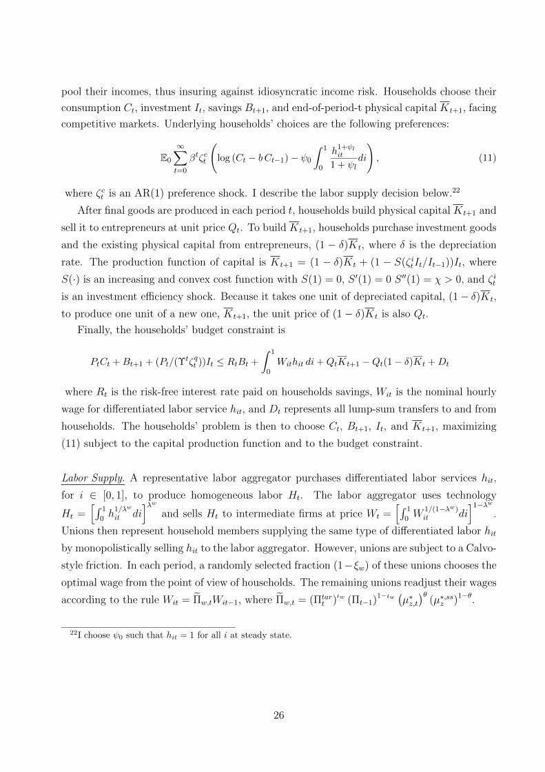
pool their incomes, thus insuring against idiosyncratic income risk. Households choose their

consumption Ct, investment It, savings Bt+1, and end-of-period-t physical capital Kt+1, facing

competitive markets. Underlying households’ choices are the following preferences:

E0

∞∑t=0

βtζct

(log (Ct − bCt−1)− ψ0

∫ 1

0

h1+ψlit

1 + ψldi

), (11)

where ζct is an AR(1) preference shock. I describe the labor supply decision below.22

After final goods are produced in each period t, households build physical capital Kt+1 and

sell it to entrepreneurs at unit price Qt. To build Kt+1, households purchase investment goods

and the existing physical capital from entrepreneurs, (1 − δ)Kt, where δ is the depreciation

rate. The production function of capital is Kt+1 = (1 − δ)Kt + (1 − S(ζ itIt/It−1))It, where

S(·) is an increasing and convex cost function with S(1) = 0, S ′(1) = 0 S ′′(1) = χ > 0, and ζ it

is an investment efficiency shock. Because it takes one unit of depreciated capital, (1− δ)Kt,

to produce one unit of a new one, Kt+1, the unit price of (1− δ)Kt is also Qt.

Finally, the households’ budget constraint is

PtCt +Bt+1 + (Pt/(Υtζqt ))It ≤ RtBt +

∫ 1

0Withit di+QtKt+1 −Qt(1− δ)Kt +Dt

where Rt is the risk-free interest rate paid on households savings, Wit is the nominal hourly

wage for differentiated labor service hit, and Dt represents all lump-sum transfers to and from

households. The households’ problem is then to choose Ct, Bt+1, It, and Kt+1, maximizing

(11) subject to the capital production function and to the budget constraint.

Labor Supply. A representative labor aggregator purchases differentiated labor services hit,

for i ∈ [0, 1], to produce homogeneous labor Ht. The labor aggregator uses technology

Ht =[∫ 1

0h

1/λw

it di]λw

and sells Ht to intermediate firms at price Wt =[∫ 1

0W

1/(1−λw)it di

]1−λw.

Unions then represent household members supplying the same type of differentiated labor hit

by monopolistically selling hit to the labor aggregator. However, unions are subject to a Calvo-

style friction. In each period, a randomly selected fraction (1−ξw) of these unions chooses the

optimal wage from the point of view of households. The remaining unions readjust their wages

according to the rule Wit = Π̃w,tWit−1, where Π̃w,t = (Πtart )

ιw (Πt−1)1−ιw (µ∗z,t)θ (µ∗,ssz )1−θ.

22I choose ψ0 such that hit = 1 for all i at steady state.

26

Government and Resource Constraint. The central bank sets its policy rate Rt according to

RtRss

=

(Rt−1

Rss

)ρr [Et(

Πt+1

Πtart

)απ (Πtart

Πss

)(∆GDPtµ∗,ssz

)αy](1−ρr)ζmpt ,

where ∆GDPt is the quarterly growth of GDP and ζmpt is a monetary policy shock. Fiscal

policy is represented by Gt following an AR(1) and by an equal amount of lump-sum taxes on

the household. For simplicity, I assume that all auditing and capital utilization costs are re-

bated as lump-sum transfers to the household. This assumption captures the idea that these

costs represent services provided by a negligible set of specialized agents who bring those

earnings to the realm of the consumption smoothing decision. Therefore, I have the following

resource constraint: Yt = Ct + It/(Υtζqt ) +Gt.

News Shocks. I allow for anticipated and unanticipated components on shocks to dispersion,

sdt, skewness, m1t , and monetary policy, ζmpt . I then model these shocks as

ζ̂t = ρζ ζ̂t−1 +4∑i=0

ξζi,t−i, ρ|i−j|ζ,ξ =

E(ξζi,tξζj,t)√

E(ξζi,t)E(ξζj,t), i, j = 0, . . . , 4,

where ζ̂t represents shocks ζmpt , sdt and m1t in log-deviation from their means, and {ξζi,t}4

i=0

measure disturbances observed by agents at time period t. I then denote ξζ0,t as the unan-

ticipated disturbance to ζ̂t and {ξζi,t−i}4i=1 as the anticipated ones, or news shocks. Distur-

bances {ξζi,t−i}4i=0 are i.i.d random variables orthogonal to {ζ̂t−i}∞i=1, with zero mean and with

E(ξ20,t) = σ2

ζ , E(ξ21,t) = . . .E(ξ2

4,t) = σ2ζ,ξ. Parameter ρζ,ξ measures the correlation between ξζi,t’s.

4.2 DSGE Model: Data, Estimation, Priors, and Posteriors

The estimation of the DSGE model uses 14 financial and macroeconomic quarterly series for

the period 1964:Q1–2015:Q2: real GDP, real consumption, real investment, hours worked,

real wage, relative investment price, the fed funds rate, core inflation, real total credit, the

real nonfinancial equity index, the spread between the Moody’s Baa rate and the 10-year

Treasury rate (Baa-10y), nonfinancial dispersion, financial skewness, and OIS expectation of

the one-year-ahead fed funds rate.23

Motivated by a potential change in structural parameters after the Great Recession and

23Quantity variables, such as GDP and credit, are transformed to per capita quarterly growth rates. Pricevariables, such as real wages and relative investment price, are expressed in quarterly growth rates, as well ascore inflation. See Appendix A.2 for details about data definitions and transformations. I include nonfinancialdispersion instead of the financial counterpart because of the evidence from Section 3.3 that it predicts debtgrowth. I then use total credit growth (loan and debt) to measure aggregate effects on credit.

27

Table 8: Parameters of the DSGE model

(a) Calibrated Parameters

Description Name Value Description Name Value

Capital share in production α 0.32 Steady-state mark-up of intermediate firms λf,ss 1.2Depreciation rate of capital δ 0.025 Labor preference ψl 1Ratio of government expenditures to GDP Gss/Y ss 0.19 Steady-state mark-up of labor unions λw 1.05Steady-state survival rate of entrepreneurs γss 0.975 Exogenous transfer to entrepreneurs1 we 0.005

Persistence of inflation trend ρπtar 0.975 Standard deviation of inflation trend σπtar

0.001

(b) Estimated Parameters

Prior distribution Posterior distributionDescription Name Shape Mean SD Mode SD

Steady-state productivity growth2 400 log(µz) invg2 1.07 0.2 0.82 0.126Investment-specific trend2 400 log(Υ) invg2 0.78 0.2 0.55 0.093Preference discount rate2 −400 log(β) invg2 1.06 0.2 0.88 0.124Steady-state inflation rate3 400 log(Πss) invg2 2 0.3 1.99 0.324Weight of GDP growth in wage indexation θ beta 0.5 0.15 0.69 0.176Calvo parameter, intermediate firms ξp beta 0.5 0.1 0.86 0.005Persistence of monetary policy rate ρr beta 0.75 0.1 0.78 0.018Weight of inflation in policy rate απ invg2 1.7 0.2 2.02 0.147Weight of GDP growth in policy rate αy beta 0.3 0.1 0.54 0.053Investment adjustment cost χ invg2 11 5 4.21 0.306Calvo parameter, labor unions ξw beta 0.75 0.1 0.92 0.011Habit persistence b beta 0.5 0.075 0.89 0.005Capital utilization cost σa invg2 2.5 2 2.01 0.713Weight of inflation trend on inflation indexation ιp beta 0.5 0.15 0.26 0.070Weight of inflation trend on wage indexation ιw beta 0.5 0.15 0.71 0.078Auditing cost µ beta 0.275 0.05 0.18 0.031Steady-state mixture probability of lognormals4 p1,ss beta 0.5 0.2 0.13 0.005Steady-state location parameter of mixture4 m1,ss normal 0 0.2 -0.05 0.003Steady-state scale parameter of mixture4 s1,ss invg2 0.2 0.1 0.10 0.004

Steady-state scale parameter of mixture4,5 αs2,ss beta 0.5 0.2 0.23 0.018

Shock autocorrelation: mark-up, intermediate firms ρλfbeta 0.5 0.2 0.03 0.045

Shock autocorrelation: preference ρζc beta 0.5 0.2 0.27 0.073Shock autocorrelation: investment price ρζq beta 0.5 0.2 0.998 0.002

Shock autocorrelation: investment efficiency ρζi beta 0.5 0.2 0.98 0.002Shock autocorrelation: government expeditures ρgov beta 0.5 0.2 0.95 0.014Shock autocorrelation: transitory TFP ρε beta 0.5 0.2 0.96 0.012Shock autocorrelation: permanent TFP ρµ∗ beta 0.5 0.2 0.25 0.063Shock autocorrelation: cross-sectional dispersion ρsd beta 0.5 0.2 0.68 0.040Shock autocorrelation: anticipated cross-sectional dispersion ρsd,ξ beta 0.5 0.2 0.53 0.163Shock autocorrelation: cross-sectional skewness ρm1 beta 0.5 0.08 0.90 0.006Shock autocorrelation: anticipated cross-sectional skewness ρm1,ξ beta 0.5 0.2 0.23 0.049Shock autocorrelation: anticipated monetary policy ρmp,ξ beta 0.5 0.2 0.83 0.044Shock standard deviation: mark-up, intermediate firms σλ invg2 0.002 0.0033 0.103 0.0035Shock standard deviation: preference σc invg2 0.002 0.0033 0.030 0.0014Shock standard deviation: investment price σq invg2 0.002 0.0033 0.005 0.0002Shock standard deviation: investment efficiency σi invg2 0.002 0.0033 0.388 0.0055Shock standard deviation: government expeditures σg invg2 0.002 0.0033 0.029 0.0015Shock standard deviation: transitory TFP σε invg2 0.002 0.0033 0.008 0.0004Shock standard deviation: permanent TFP σµ∗ invg2 0.002 0.0033 0.015 0.0017Shock standard deviation: cross-sectional dispersion σsd invg2 0.002 0.0033 0.037 0.0022Shock standard deviation: anticipated cross-sectional dispersion σsd,ξ invg2 0.001 0.0012 0.0003 0.0002Shock standard deviation: cross-sectional skewness σm1 invg2 0.002 0.0033 0.046 0.0036Shock standard deviation: anticipated cross-sectional skewness σm1,ξ invg2 0.001 0.0012 0.037 0.0010Shock standard deviation: monetary policy σmp invg2 0.002 0.0033 0.001 0.0001Shock standard deviation: anticipated monetary policy σmp,ξ invg2 0.001 0.0012 0.001 0.0001Shock standard deviation: equity σγ,e invg2 0.002 0.0033 0.033 0.0017Measurement error: dispersion σdisp,obs invg2 0.005 0.01 0.003 0.0032Measurement error: skewness σskew,obs invg2 0.005 0.01 0.015 0.0020Measurement error: equity proportion6 Γ invg2 1 0.5 0.23 0.007Measurement error: equity6 σeq invg2 0.001 0.05 0.092 0.0053Measurement error: real wages σw,obs invg2 0.001 0.05 0.006 0.0004

All shock autocorrelations and standard deviations are estimated in 2 steps, as described in Section 4.2. Remaining parameters are fixed at the

mode found in the estimation with the 1964-2006 sample (1st step). “invg2” is the inverse gamma distribution, type 2. 1Steady-state We,ss is

calibrated as a percentage we of the steady-state capital stock Kss (normalized by its growth trend). 2These parameters are only estimated in

the 2nd stage, while being fixed at their sample means during the 1st stage. 3It is only estimated in the 1st step, being fixed at 2 in the 2nd

step. 4Although I renormalize Ft from (m1t , s

1,ss,m2t , s

2,ss, p1t ) to (m1t , s

1,ss, sdt, s2,ss), I pin down the steady state of Fss by estimating

(m1,ss, s1,ss, s2,ss, p1,ss), where m2,ss is such that∫ωdFss(ω) = 1. 5To achieve identification, I estimate s2,ss as a percentage αs2,ss of

s1,ss. 6I assume that observed equity growth is Γ times model equity growth plus a measurement error.

28

Table 9: Data Averages and Steady State Moments from the Model

Description Model DataConsumption GDP ratio 0.55 0.55Investment GDP ratio 0.26 0.25Capital GDP ratio 9.03 10.9a

Inflation (APR) 2 3.41Monetary policy interest rate 4 5.29Leverage of entrepreneurs 5 1.7-15.3b

aFrom Christiano et al (2014). bThese are aggregate measures, where the lower bond is for nonfinancial businesses and theupper bound is for the domestic financial sector. Source: Financial Accounts, Federal Reserve Board.

by the adoption of a more explicit guidance about future policy rates by the Fed, I use a

two-step estimation procedure. In the first step, I estimate model parameters using data

for the period 1964:Q1–2006:Q4, excluding OIS-rates and imposing a white noise structure

on monetary policy shocks ζmpt . I calibrate some model parameters, postulate priors for the

remaining parameters, and then maximize the log-posterior of the model. In the second

step, I re-estimate the persistence and standard deviation of all shocks, using data for the

period 2002:Q1–2015:Q2, including OIS-rates and allowing for anticipated and unanticipated

monetary policy shocks. Additionally, in the second estimation step, I (i) fix at the first-step

mode all parameters not re-estimated in the second step, (ii) center the prior of re-estimated

parameters on the first-step mode, (iii) choose the standard deviation of the prior of re-

estimated parameters to be the standard deviation of the first-step posterior, and (iv) impose

a zero auto-correlation ρmp for monetary policy shocks.24 The focus of this two-step procedure

on the persistence and size of economic shocks lowers the number of parameters estimated

twice and is consistent with the evidence provided by Stock and Watson (2012). They argue

that the 2008 recession was the result of large versions of shocks already experienced and that

the response of macro variables was in line with historical standards.

Table 8 documents calibrated values as well as prior and posterior distributions of all

parameters. Most estimated parameters are within the range of estimates reported in the

literature. However, the parameters determining the steady-state distribution of idiosyncratic

asset returns F ss pin down a distribution markedly different from the lognormal case, which

is largely assumed in the financial frictions literature. Figure 7 reports F ss (black line) and a

lognormal distribution with identical mean and standard deviation (green line). We then see

that the tails of F ss are much fatter than the ones of the lognormal distribution, especially

the left one. Finally, Table 9 documents the steady state of several model variables, showing

24The reason for having an overlapping period between the samples used by the two estimation steps isto dilute the influence of a particular break-date. Additionally, I include measurement errors in real wagegrowth, equity growth, cross-sectional dispersion, and cross-sectional skewness.

29

that they are close to most of their data counterparts.25

4.3 The Primacy of Skewness Shocks in The DSGE Model

Skewness shocks are the most important driver of economic fluctuations in the DSGE model, as

shown in the variance decomposition of Table 10. It shows that skewness shocks, anticipated

and non-anticipated, account for 48% of fluctuations in GDP growth and similarly large

numbers for other endogenous variables, such as 60% for investment growth, 41% for credit

growth, and 66% for Baa-10y spread. We also see that the anticipated portion of shocks to

skewness account for the majority of their explanatory power. Shocks to TFP, investment

cost, equity, and monetary policy have moderate explanatory power for business cycles. In

contrast, dispersion shocks become essentially irrelevant. Finally, the skewness measure is

mostly exogenous, while dispersion is mostly endogenous.

Table 10: Variance Decomposition from the DSGE Model1 (Percent)

ShocksInv-Cost TFP Equity MP MP-News Disp Disp-News Skew Skew-News

Variables ζit εt, µ∗t γt ξmp0,t {ξ

mpi,t−i}4i=1 ξsd0,t {ξsdi,t−i}4i=1 ξm

1

0,t {ξm1

i,t−i}4i=1

GDP2 12 18 1 0 15 0 0 7 41Consumption2 26 17 2 0 13 0 0 5 32Investment2 11 10 2 0 16 0 0 9 51Credit2 33 7 9 0 7 0 0 6 35Equity2,3 18 0 1 0 1 0 0 1 4Baa-10y 29 0 2 0 2 0 0 16 50Dispersion 53 1 3 0 3 11 4 4 19Skewness 1 0 0 0 0 5 2 19 74

1Percentages do not add to 100 because remaining shocks account for the residual. 2Variables used in four quarter growth.3Measurement error accounts for a large variability of this variable.

Figure 8 shows that skewness shocks are important economic drivers regardless of the

state of the cycle. It shows both the data of GDP growth, investment growth, credit growth,

and Baa-10y spread (in red) and how these variables would have evolved if only skewness

shocks had impulsed the economy (in blue). The difference between the blue and red series

is accounted for by the contribution of all the other shocks used in the estimation. We then

see that skewness shocks were major contributors to all expansions and recessions throughout

the period 1964–2015. We also see that variations in credit spreads are largely explained by

skewness shocks and that these shocks account for low frequency movements in credit growth.

25Appendix A.4 also documents that the marginal likelihood of this DSGE model is close to the one froma BVAR with the same time series and sample period.

30

Figure 8: Shock Decomposition, 1964–2015

(a) GDP 4Q growthP

erce

ntag

e

-8

-6

-4

-2

0

2

4

6

Q1-1964

Q4-1969

Q3-1975

Q1-1981

Q4-1986

Q3-1992

Q2-1998

Q1-2004

Q3-2009

Q2-2015

DataAnticipated and Unanticipated Skewness Shocks

(b) Investment 4Q growth

Per

cent

age

-25

-20

-15

-10

-5

0

5

10

15

Q1-1964

Q4-1969

Q3-1975

Q1-1981

Q4-1986

Q3-1992

Q2-1998

Q1-2004

Q3-2009

Q2-2015

DataAnticipated and Unanticipated Skewness Shocks

(c) Credit 4Q growth

Per

cent

age

-10

-8

-6

-4

-2

0

2

4

6

8

Q1-1964

Q4-1969

Q3-1975

Q1-1981

Q4-1986

Q3-1992

Q2-1998

Q1-2004

Q3-2009

Q2-2015

DataAnticipated and Unanticipated Skewness Shocks

(d) Baa-10y Spread

Per

cent

age

-2

-1

0

1

2

3

4

Q1-1964

Q4-1969

Q3-1975

Q1-1981

Q4-1986

Q3-1992

Q2-1998

Q1-2004

Q3-2009

Q2-2015

DataAnticipated and Unanticipated Skewness Shocks

31

Figure 9: Impulse Response Functions from BVARs and DSGE model

(a) Skewness Shocks (b) Dispersion Shocks

32

Impulse response functions (IRFs) in Figure 9 shed light on the reason skewness shocks are

important drivers of business cycle fluctuations. Essentially, when cross-sectional skewness is

exogenously lower, endogenous variables respond with co-movements generally observed over

the cycle (black lines in Figure 9a): higher credit spreads and dispersion, and then lower credit,

equity, investment, consumption, and GDP growth. Similarly to Christiano et al. (2014), most

other shocks do not generate this entire set of co-movements, and thus are not able to account

for large shares of business cycle fluctuations.26 The exception to this argument in this paper

are dispersion shocks, shown in Figure 9b.

The question then becomes why skewness shocks are more related to the business cycle

than dispersion ones. The answer comes from comparing Figures 9a and 9b. Although IRFs to

skewness and dispersion shocks follow qualitatively similar dynamics, skewness shocks cause

much stronger effects to endogenous variables. A one standard deviation exogenous drop in

skewness increases the Baa-10y spread by 35 basis points and dispersion by about 4.5% at

their peaks, while it decreases credit growth by 0.4%, equity growth by 1%, investment growth

by 2%, consumption growth by 0.3%, and GDP growth by 0.8% at their troughs. In contrast,

these variables barely react to a one standard deviation exogenous increase in dispersion, with

the exception of dispersion itself.

Skewness shocks have stronger effects on the economy than dispersion shocks because of

two factors. First, entrepreneurial bankruptcy is more reactive to changes in skewness than to

changes in dispersion. To see this argument at its simplest form, I ignore general equilibrium

effects and (i) decrease by one standard deviation the steady-state value of the skewness

parameter from m1,ss to m̃1,ss, (ii) keep fixed the threshold ωss at its steady-state level as well

as all the other parameters of F ss, and (iii) graph the change in entrepreneurial bankruptcy

(i.e., from F(ωss;m1,ss, ·) to F(ωss; m̃1,ss, ·)). I also implement an analogous exercise to steady-

state cross-sectional dispersion sdss. Figure 7a displays these exercises. The comparison of

the increase in bankruptcy due to changes in skewness and dispersion reveals a much higher

elasticity to changes in skewness. The second factor is that skewness shocks m1t are much

more persistent than dispersion ones sdt, as seen in Table 8b.

In general equilibrium, these two factors then increase the effects of skewness shocks,

relative to dispersion ones, by amplifying the channel through which both of these shocks

affect the economy. More specifically, there is a larger and more persistent increase in the mass

of entrepreneurs with low asset returns and, in turn, higher and more persistent bankruptcy

26I report the IRFs of other shocks, including anticipated skewness shocks, in Appendix A.3. There wesee that shocks such as investment efficiency have difficulty in matching co-movements of not only creditoutstanding and credit spreads (as in Christiano et al. (2014)), but also of the series of cross-section dispersionand skewness.

33

losses (IRFs in lower right of Figures 9a and 9b); mutual funds magnify their decreases in

the amount of credit and their increases in loan interest rates to compensate for these higher

losses; equity drops more; and investment and GDP contract more decisively, which then lead

to several other larger general equilibrium effects described by Figures 9a and 9b.

4.4 Identification of Shocks in the BVARs

In addition to estimating a DSGE model, I also identify financial skewness shocks using

BVARs. The goal of using different frameworks is to reach robust conclusions about the

importance of skewness shocks to business cycles as well as about the transmission of these

shocks through the economy. I use the same data as in the estimation of the DSGE model

(Section 4.2), except that I exclude OIS rates because they only start at 2002.27

In the BVARs, I identify unanticipated skewness shocks with four strategies: three different

recursive orderings and one identification strategy based on the DSGE model. I define Order-

13 as the recursive ordering placing skewness last in the BVAR, thus allowing the remaining

variables to react to a skewness shock only with one quarter of lag. I define Order-10 as

the ordering placing skewness before equity growth, Baa-10y spread, and dispersion, thus

allowing these variables to react contemporaneously to a skewness shock, while only letting

the remaining variables react to the shock with one quarter of lag. I also define Order-1 as

the ordering placing skewness as the first variable, thus allowing all remaining variables to

react contemporaneously to a skewness shock.

The strategy for identifying skewness shocks based on the DSGE model is named BVAR-

DSGE and it works as follows. I build a vector of contemporaneous responses of all BVAR

variables to a skewness shock.28 Then, I pin down the magnitude of the responses in this

vector by using the contemporaneous responses of the same variables to an unanticipated

skewness shock estimated by the DSGE model. For completeness, I also identify dispersion

shocks using analogous recursive and BVAR-DSGE strategies.

The reason for using the BVAR-DSGE identification is to provide a cleaner comparison

between the DSGE model and the BVARs. To see this, notice that the economic analysis of

a shock in either the DSGE model or the BVARs may be divided in two components: the

economic effects of the shock at the time period of its arrival (impulse), and the propagation

of the impulse through the economy over time (propagation mechanism). Thus, when we

compare, for instance, the IRFs to skewness shocks from the DSGE model with those from

27I use the BVAR with Minnesota prior and optimal shrinkage from Giannone et al. (2015).28Uhlig (2005) shows that a sufficient condition to exactly identify a shock is to pin down a vector of

contemporaneous responses of all BVAR variables to the desired shock.

34

recursive identifications, we compare not only different impulses, but also different propaga-

tion mechanisms. Alternatively, when we compare IRFs to skewness shocks from the DSGE

model with those from the BVAR-DSGE identification, we focus only on the differences in

propagation mechanisms.

4.5 DSGE Model and BVARs: The Prominence of Skewness Shocks

Skewness shocks have sizable and long-lasting economic effects, account for a relevant share

of business cycles, and explain the majority of the fluctuations in financial skewness. I reach

these conclusions by focusing on results from IRFs and variance decompositions that are

robust across the DSGE model and the many identifications used in the BVARs.

More precisely, the conclusions above originate from three results. First, IRFs (Figure 9a)

to unanticipated skewness shocks have a considerable effect on GDP growth, decreasing it for

at least six quarters and by 0.3-0.8% at the troughs. Moreover, results for other measures of

economic activity, such as consumption and investment, show similarly strong effects. Second,

variance decompositions of GDP growth (Tables 10 and 11a) show that unanticipated skewness

shocks account for 5-20% of the fluctuations in this variable, with shares for investment

and consumption being of similar magnitudes. Third, variance decompositions of financial

skewness show that it is largely an exogenous variable. Skewness shocks (anticipated and

unanticipated) are responsible for almost all of the variance of financial skewness in the DSGE

model (Table 10) and unanticipated skewness shocks explain between 54% to 74% in the

BVAR’s recursive identifications.

Table 11: Variance Decompositions from BVARs (Percent)

(a) Skewness Shocks

IdentificationsVariables Order-1 Order-10 Order-13 BVAR-DSGEGDP1 20 7 5 9Consumption1 19 6 4 6Investment1 20 7 4 7Credit1 20 9 5 5Equity1 21 14 4 3Baa-10y 16 8 4 39Dispersion 13 7 3 8Skewness 74 63 54 22

(b) Dispersion Shocks

IdentificationsOrder-1 Order-10 Order-13 BVAR-DSGE

3 2 2 33 2 2 35 3 2 414 9 7 124 3 2 310 8 4 548 43 35 276 5 2 31

1Variables used in 4 quarter growth.

In contrast, dispersion shocks have almost negligible economic effects, account for a very

small share of business cycles, and explain only a modest share of the fluctuations in the

35

observed dispersion measure. All of these conclusions are also robust across the DSGE model

and the many identifications used in the BVARs. I reach these conclusions with the following

three results: (i) IRFs to dispersions shocks are not different from zero (Figure 9b), (ii)

the contribution of dispersion shocks to fluctuations in GDP, investment and consumption

are 0-5% (Tables 10 and 11b), and (iii) dispersion shocks account for less than half of the

fluctuations in the observed dispersion measure (Tables 10 and 11b).

4.6 The Transmission of Skewness Shocks

I then provide evidence that financial frictions is an important transmission channel of financial

skewness shocks.

4.6.1 The Larger The Response of Credit Spreads, The Larger The Macro Effects

I do so by first showing that the larger the effect of skewness shocks on credit spreads, the

larger the effect on economic activity. This result comes from looking at the IRFs in Figure 9a

in the following progression of identification strategies: Order-13, Order-10, Order-1, BVAR-

DSGE, and DSGE. First, we observe that the response of Baa-10y spread to skewness shocks

is increasing in this progression of identifications, with the IRF peak increasing from 6 basis

points to 35 basis points. Then, we observe an increasing response of economic activity in

this progression of IRFs, with the trough of GDP growth decreasing from negative 0.3% to

negative 0.8%. Investment and consumption growth also follow similar patterns.

Although the results above are consistent with financial frictions being a powerful amplifier

of skewness shocks, they do not rule out other transmission channels for these shocks. For

instance, the IRF of the Order-13 identification (Figure 9a) shows skewness shocks decreasing

GDP growth by 0.3% while credit spreads only increase by 6 basis points, a result consistent

with a nonfinancial transmission channel such as capital frictions (Ehouarne et al. (2015)).

4.6.2 Financial Accelerator Is Channel Mostly Consistent with The BVAR

I then provide further support for the importance of financial frictions in transmitting skewness

shocks by showing evidence consistent with the financial accelerator channel of the DSGE

model: After unexpected decreases in financial skewness, credit conditions tend to quickly

tighten (lower credit and equity growth, and higher credit spreads), with investment and

GDP contracting in the following quarters.

I provide the evidence above by comparing the IRFs to unanticipated skewness shocks

estimated by the DSGE model with the IRFs identified by the BVAR-DSGE procedure.

36

Intuitively, this exercise compares the transmission of a specific financial skewness shock in

two different model economies: one agnostically maximizing its data fit through a BVAR, and

another that also maximizes its data fit while being restricted to have a financial accelerator

channel. This comparison (Figure 9a) shows that IRFs of measures of economic activity (GDP,

consumption, and investment) under the BVAR-DSGE identification are similar to those from

the DSGE model, with the latter being somewhat larger. This comparison also shows that

IRFs from the DSGE model for most financial variables (credit, equity, Baa-10y spread, and

dispersion) often lie inside the probability intervals of the BVAR-DSGE IRFs.

Although the comparison of IRFs above provides support for the financial accelerator

channel of financial skewness shocks, it also shows one limitation of this model. While it takes

approximately only 3 quarters for financial skewness to return to its level prior to the shock

in the BVAR-DSGE, it takes more than 16 quarters in the DSGE model. This discrepancy

suggests that the DSGE model lacks an internal mechanism that can transmit skewness shocks

throughout the economy for many periods after the shock dissipates.

5 Conclusion

In this paper, I argue that financial skewness—the cross-sectional skewness of the distribution

of stock market returns of financial firms—is an empirical measure with considerable poten-

tial to both predict and explain business cycle fluctuations. I support this argument with

three main results. First, using data from 1926 to 2015, I show that financial skewness not

only closely track business cycles, but also predicts economic activity better than well-known

indicators. Second, I provide evidence supporting the hypothesis that the predictive ability of

financial skewness originates from the exposure of financial firms to the economic performance

of their borrowers. Third, I show that shocks to financial skewness are important drivers of

business cycles using both BVARs and a DSGE model.

This paper points to two avenues of future research. First, one investigating how high-

order moments of asset prices may shed light on understanding business cycle fluctuations.

Second, a research path in which the financial sector not only is the origin of shocks to the

economy (e.g., the 1929 and 2008 financial crises), but also is well placed to efficiently signal

shocks from other sectors. Thus, papers investigating these issues on additional asset prices,

such as bonds, and theoretical models microfounding the signaling power of financial firms

are important examples of tasks for future research.

37

References

[1] Abadir, Karim M., and Paolo Paruolo. “Two mixed normal densities from cointegration

analysis.” Econometrica 65, no. 3 (1997): 671-680.

[2] Acemoglu, Daron, Vasco M. Carvalho, Asuman Ozdaglar, and Alireza Tahbaz-Salehi.

“The network origins of aggregate fluctuations.” Econometrica 80, no. 5 (2012): 1977-

2016.

[3] Arellano, Cristina, Yan Bai, and Patrick J. Kehoe. “Financial frictions and fluctuations

in volatility.” No. w22990. National Bureau of Economic Research, 2016.

[4] Bachmann, Rdiger, and Christian Bayer. “Investment dispersion and the business cycle.”

The American Economic Review 104, no. 4 (2014): 1392-1416.

[5] Barro, Robert J. “Rare disasters and asset markets in the twentieth century.” The Quar-

terly Journal of Economics 121, no. 3 (2006): 823-866.

[6] Bassett, William F., Mary Beth Chosak, John C. Driscoll, and Egon Zakrajsek. “Changes

in bank lending standards and the macroeconomy.” Journal of Monetary Economics 62

(2014): 23-40.

[7] Bekaert, Geert, Marie Hoerova, and Marco Lo Duca. “Risk, uncertainty and monetary

policy.” Journal of Monetary Economics 60, no. 7 (2013): 771-788.

[8] Bernanke, Ben S., Mark Gertler, and Simon Gilchrist. “The financial accelerator in a

quantitative business cycle framework.” Handbook of Macroeconomics 1 (1999): 1341-

1393.

[9] Bloom, Nicholas, Max Floetotto, Nir Jaimovich, Itay Saporta-Eksten, and Stephen J.

Terry. “Really uncertain business cycles.” No. w18245. National Bureau of Economic

Research, 2012.

[10] Bloom, Nicholas. “Fluctuations in uncertainty.” The Journal of Economic Perspectives

28, no. 2 (2014): 153-175.

[11] Bloom, Nicholas, Fatih Guvenen, and Sergio Salgado. “Skewed Business Cycles.” In 2016

Meeting Papers, no. 1621. Society for Economic Dynamics, 2016.

[12] Brave, Scott A., and R. Andrew Butters. “Monitoring financial stability: A financial

conditions index approach.” (2011).

[13] Caldara, Dario, Cristina Fuentes-Albero, Simon Gilchrist, and Egon Zakrajek. “The

macroeconomic impact of financial and uncertainty shocks.” European Economic Review

88 (2016): 185-207.

38

[14] Christiano, Lawrence J., Roberto Motto, and Massimo Rostagno. “Risk shocks.” The

American Economic Review 104, no. 1 (2014): 27-65.

[15] Chugh, Sanjay K. “Firm risk and leverage-based business cycles.” Review of Economic

Dynamics 20 (2016): 111-131.

[16] Diebold, Francis X., and Robert S. Mariano. “Comparing Predictive Accuracy.” Journal

of Business & Economic Statistics 13 (1995): 253-263.

[17] Ehouarne, Cedric, Lars-Alexander Kuehn, and David Schreindorfer. “The Market Price

of Capital Misallocation.” (2015).

[18] Fama, Eugene F., and Kenneth R. French. “Common risk factors in the returns on stocks

and bonds.” Journal of Financial Economics 33, no. 1 (1993): 3-56.

[19] Ferreira, Thiago RT. “Financial Volatility and its Economic Effects.” Working paper

(2016).

[20] Gabaix, Xavier. “The granular origins of aggregate fluctuations.” Econometrica 79, no.

3 (2011): 733-772.

[21] Gabaix, Xavier. “Variable rare disasters: An exactly solved framework for ten puzzles in

macro-finance.” The Quarterly Journal of Economics (2012): qjs001.

[22] Giannone, Domenico, Michele Lenza, and Giorgio E. Primiceri.“Prior selection for vector

autoregressions.” Review of Economics and Statistics 97, no. 2 (2015): 436-451.

[23] Gilchrist, Simon, and Egon Zakrajek. “Credit spreads and business cycle fluctuations.”

The American Economic Review 102, no. 4 (2012): 1692-1720.

[24] Gilchrist, Simon, Jae W. Sim, and Egon Zakrajek. “Uncertainty, financial frictions, and

investment dynamics.” No. w20038. National Bureau of Economic Research, 2014.

[25] Gourio, Francois. “Disaster risk and business cycles.” The American Economic Review

102, no. 6 (2012): 2734-2766.

[26] Guvenen, Fatih, Serdar Ozkan, and Jae Song. “The nature of countercyclical income

risk.” Journal of Political Economy 122, no. 3 (2014): 621-660.

[27] Hodrick, Robert J. “Dividend yields and expected stock returns: Alternative procedures

for inference and measurement.” Review of Financial Studies 5, no. 3 (1992): 357-386.

[28] Kelly, Bryan, and Hao Jiang. “Tail risk and asset prices.” Review of Financial Studies

27, no. 10 (2014): 2841-2871.

[29] Kiefer, Nicholas M., Timothy J. Vogelsang, and Helle Bunzel. “Simple robust testing of

regression hypotheses.” Econometrica 68, no. 3 (2000): 695-714.

39

[30] Kiefer, Nicholas M., and Timothy J. Vogelsang. “Heteroskedasticity-autocorrelation ro-

bust standard errors using the Bartlett kernel without truncation.” Econometrica 70, no.

5 (2002): 2093-2095.

[31] Jurado, Kyle, Sydney C. Ludvigson, and Serena Ng. “Measuring uncertainty.” The Amer-

ican Economic Review 105, no. 3 (2015): 1177-1216.

[32] Lopez-Salido, David, Jeremy C. Stein, and Egon Zakrajsek. “Credit-market sentiment

and the business cycle.” The Quarterly Journal of Economics (2017): qjx014.

[33] Ludvigson, Sydney C., Sai Ma, and Serena Ng. “Uncertainty and Business Cycles: Ex-

ogenous Impulse or Endogenous Response?” No. w21803. National Bureau of Economic

Research, 2015.

[34] Luo, Shaowen and Daniel Villar Vallenas. “The Skewness of the Price Change Distribu-

tion: A New Touchstone for Sticky Price Models.” No. 2017-028. Board of Governors of

the Federal Reserve System (US), 2017.

[35] Ng, Serena, and Jonathan H. Wright. “Facts and Challenges from the Recession for

Forecasting and Macroeconomic Modeling.” Journal of Economic Literature 51, no. 4

(2013): 1120-1154.

[36] Panousi, Vasia, and Dimitris Papanikolaou. “Investment, idiosyncratic risk, and owner-

ship.” The Journal of Finance 67, no. 3 (2012): 1113-1148.

[37] Philippon, Thomas. “The bond market’s q.” The Quarterly Journal of Economics 124,

no. 3 (2009): 1011-1056.

[38] Schaal, Edouard. “Uncertainty and unemployment.” Econometrica 85, no. 6 (2017): 1675-

1721.

[39] Stock, James H., and Mark W. Watson. “Forecasting output and inflation: The role of

asset prices.” Journal of Economic Literature 41, no. 3 (2003): 788-829.

[40] Stock, James H., and Mark W. Watson. “Disentangling the Channels of the 2007-2009

Recession.” No. w18094. National Bureau of Economic Research, 2012.

[41] Zeke, David. “Financial Frictions, Volatility, and Skewness.” mimeo, University of

California-Los Angeles, 2016.

40

A Appendix

A.1 Classification: Financial and Nonfinancial Sectors

This section is reproduced from Ferreira (2016). In order to classify the firms as financial or non-

financial, I use all the information available in the sample. On the one hand, CRSP provides the

most recent U.S. Census classification, NAICS, and an older one, SIC. On the other hand, there

is an SIC code for all firms, while the NAICS is available only for some. To avoid an outdated

classification procedure of an ever-changing financial sector, I place an emphasis on the NAICS clas-

sification. Moreover, since this study focuses on private financial firms, I look for those with the

following three-digit NAICS classifications: 522 (Credit Intermediation and Related Activities), 523

(Securities, Commodity Contracts, and Other Financial Investments and Related Activities), 524

(Insurance Carriers and Related Activities), and 525 (Funds, Trusts, and Other Financial Vehicles).

With these issues in mind, I adopt the following classification procedure:

(a) for those firms with a NAICS code available, I classify:

(a1) as financial those with codes 522, 523, 524, or 525;

(a2) as nonfinancial those with codes other than those above;

(b) for those firms without a NAICS code, I use information from the U.S. Census website about

bridging the two classifications to find the SIC codes associated with the 3-digit NAICS codes

522, 523, 524, or 525. Then, I follow procedures (a1) and (a2).

A.2 Data Used by BVAR and DSGE Models

1. Core inflation is calculated using the price index of personal consumption expenditures (PCE)

that excludes food and energy.

2. Real GDP is calculated by deflating nominal GDP by the implicit GDP price index and by the

population over 15 years old.

3. Real consumption is the sum of nominal PCE in services and non-durables, deflated by the

PCE price index and by the population over 15 years old.

4. Real investment is the sum of nominal PCE in durables and nominal business investment,

deflated by the business investment price index and by the population over 15 years old.

5. Real wage is measured by the hourly compensation of all employees in non-farm business,

deflated by the core PCE price index.

6. Relative investment price is calculated as the ratio between the business investment price index

and the core PCE price index.

41

7. Real credit is sum of loans (depository institutions loans nec, other loans and advances and

total mortgages) and debt (commercial paper, municipal securities, corporate bonds) from the

financial accounts (liabilities of nonfinancial businesses) published by the Board of Governors

of the Federal Reserve System. It is then normalized by the core PCE price index and by the

population over 15 years old.

8. Nonfinancial equity index is the cumulative weighted return of all nonfinancial firms, normalized

by the core PCE price index and by the population over 15 years old.

9. Hours worked is measured by the aggregate weekly hours of production and non-supervisory

employees in all private industries, divided by the population over 15 years old.

10. Fed funds rate is the average of the daily rates over the quarter.

11. Baa-10y spread is measured by the spread between the Moody’s Baa rate and the 10-year

Treasury rate.

12. Nonfinancial dispersion is calculated as described in Section 2.

13. Financial skewness are calculated as described in Section 2.

I then take the growth rates of variables (2)-(8), while keeping variables (9)-(13) at their quarterly

levels. Finally, I demean these variables as follows: (i) for the period 1964-1985, I divide the variable

by its mean within this subsample; (ii) for the period 1986-2015, I divide the variable by its mean

within this subsample; and (iii) I splice the demeaned series from (i) and (ii). This demeaning

procedure is done to account for the evidence that long-run growth for the United States has decreased

since the 1960s and for the evidence of a structure break around 1985 due to the Great Moderation.

Given that I include inflation trend in the dynamic stochastic general equilibrium (DSGE) model, I

exclude inflation, fed funds, and OIS rates from this demeaning process.

A.3 Additional Results

42

Table 12: In-Sample GDP Forecast Regressions, Four Quarters Ahead, 1973–2015

(a) Financial Firms, Weighted Distribution Measures

Regressions SpecificationsVariable (1) (2) (3) (4) (5) (6) (7) (8) (9) (10) (11) (12)

Mean 1.01*** 0.51**Dispersion -0.42* -0.15Skewness 1.11*** 1.17*** 0.92***Left kurtosis 0.63 -0.38Right kurtosis 0.39*** -0.28***Uncertainty -0.46** 0.08Real fed funds -0.44 0.02Term spread 0.92*** 1.04***GZ spread -0.55** -0.50R2 0.08 0.23 0.13 0.26 0.13 0.11 0.19 0.12 0.28 0.23 0.32 0.53

(b) Nonfinancial Firms, Weighted Distribution Measures

Regressions SpecificationsVariable (1) (2) (3) (4) (5) (6) (7) (8) (9) (10) (11) (12)

Mean 0.94*** 0.89*** 0.61*Dispersion -0.30 -0.41Skewness 0.50** -0.91Left kurtosis 0.47** 0.37Right kurtosis 0.51** 0.82Uncertainty -0.46** 0.12Real fed funds -0.44 -0.01Term spread 0.92*** 0.98***GZ spread -0.55** -0.69R2 0.08 0.21 0.11 0.12 0.12 0.12 0.19 0.12 0.28 0.23 0.26 0.49

This table reports the results from regression (6) on average GDP growth four quarters ahead (h = 4), with p = 4 because of the relatively low

AIC of this specification, and q = 1 to keep the model parsimonious. Real fed funds is measured by the fed funds rate minus the four-quarter

change of core inflation from the personal consumption expenditures. The elasticities of regressor variables reported above are calculated by

summing the contemporaneous and lagged coefficients of each regressor,{βk =

∑qj=0 β

kj

}5

k=1and γ =

∑qj=0 γj. Coefficients of lagged GDP

growth are omitted. Standard errors are calculated according to Hodrick (1992). Statistical significance tests the null hypothesis that all

coefficients associated to a regressor equal to zero, where ∗, ∗∗, and ∗ ∗ ∗ denote significance levels of 0.1, 0.05, and 0.01.

43

Table 13: In-Sample Forecast Regressions, Credit Variables, Four Quarters Ahead, 1973–2015

(a) Notation

(1) Benchmark R2

(2)Bivariate

Variable(3) R2

(4)

Multivariate

Variable(5) Uncertainty(6) Real fed funds(7) Term spread(8) GZ spread(9) R2

(b) Variable = Financial Dispersion

Loans Debt Loan Sp(bp) GZ Sp(bp) Baa-10Y(bp)

0.57 0.40 0.88 0.84 0.78

-2.35*** 0.18* 4.69*** -0.85*** 6.99***

0.69 0.41 0.89 0.88 0.82

-2.12* 0.69* 1.95 -4.89*** 2.52***0.44* 0.28 5.79*** 9.06*** 6.66*

-0.32 0.49 -8.87* -1.41* -2.67***0.51 0.14 0.14 0.78 -1.74***

-1.97** -1.47***

0.81 0.56 0.90 0.89 0.86

(c) Variable = Nonfinancial Skewness

Loans Debt Loan Sp(bp) GZ Sp(bp) Baa-10Y(bp)

0.57 0.40 0.88 0.84 0.78

1.74*** 0.29 -4.06* -16.83*** -18.63***

0.64 0.40 0.88 0.87 0.83

0.35 -0.37 -2.21 -15.98*** -15.57***-0.68 0.65 6.20*** 8.36*** 8.57***-0.88* 0.55 -5.53 -5.29** -3.08***0.16 0.26 2.23 -2.04 -1.90**

-1.84 -1.56***

0.76 0.55 0.90 0.89 0.87

This table reports the results from regression 6 on loan growth, debt growth, loan spread, GZ spread, and Baa-10y spread. Loan and debt are taken from the Flow of Funds,nonfinancial business balance sheet, levels. Loan spread is from the Survey of Terms of Business Lending of the Federal Reserve. Loan, GZ, and Baa-10y spreads are used in levels.I use h = 4, p = 4 because of the relatively low AIC of this specification, and q = 1 to keep the model parsimonious. Real fed funds is measured by the fed funds rate minusthe four-quarter change of core inflation from the personal consumption expenditures. Uncertainty refers to the financial uncertainty calculated by Ludvigson et al. (2016). The

elasticities of regressor variables reported above are calculated by summing the contemporaneous and lagged coefficients of each regressor,{βk =

∑qj=0 β

kj

}5

k=1and γ =

∑qj=0 γj.

Elasticities on loan and debt growth is expressed in percentage, while on spreads is in basis points. Coefficients of lagged predicted variables are omitted. Standard errors arecalculated according to Hodrick (1992). Statistical significance tests the null hypothesis that all coefficients associated to a regressor equal to zero, where ∗, ∗∗, and ∗ ∗ ∗ denotesignificance levels of 0.1, 0.05, and 0.01.

44

A.4 The DSGE Model Is Statistically Comparable to BVAR

The first column of Table 14 shows that the marginal likelihood of the DSGE model from

Section 4 is close to the one from a BVAR using the same time series and sample period

(2002–2015). However, the second and third columns of Table 14 show that if we exclude

OIS rates from the estimation of the DSGE model and focus on either the entire sample

(1964–2015) or the pre-Great-Recession era (1964–2006), the marginal likelihood of the DSGE

model becomes considerably lower than those from BVARs with identical data.

Table 14: Marginal Likelihood (Log Points)

Sample 2002-2015 1964-2006 1964-2015DSGEa 2178 6154b 7374b

BVARc 2158 6368 7672aIt is computed by the Modified Harmonic Mean method from a Markov Chain Monte Carlo with 2 blocks, each with 300,000draws. b In these estimations, I use standard Bayesian methods without the two-step procedure used for the baseline modeland exclude the OIS rates from the estimation. cIt uses the exact same data as the DSGE model and it is computed from aBVAR with Minnesota prior and optimal shrinkage, as in Giannone et al (2015).

These results from Table 14 support the choice of Section 4’s DSGE model and its esti-

mation procedure as a reasonable starting point to study the transmission of skewness shocks

through financial frictions. This argument is based on the fact that the performance of the

DSGE model, relative to a BVAR, is best exactly when there is more evidence that financial

frictions contributed to a cyclical downturn of the U.S. economy.

45

Figure 10: Impulse Response Functions

4 8 12 16

% D

evia

tion

from

initi

al le

vel

-1.5

-1

-0.5

0Real GDP

4 8 12 16-1.5

-1

-0.5

0

0.5Consumption

4 8 12 16-4

-3

-2

-1

0Investment

4 8 12 16

% D

evia

tion

from

initi

al le

vel

-2

-1

0

1

2Credit

4 8 12 16-5

0

5

10

15

20

25Equity

4 8 12 16-0.4

-0.2

0

0.2

0.4Baa spread (APR)

quarters after the shock4 8 12 16

% D

evia

tion

from

initi

al le

vel

-15

-10

-5

0

5

10Dispersion

quarters after the shock4 8 12 16

-8

-6

-4

-2

0

2Skewness

Skewness shockDispersion shockInv-cost. shockEquity shockSkew-News shock

46