W. Rohringer, D. Fischer, M. Trupke, J. Schmiedmayer, T. SchummVienna Center for Quantum Science and Technology, Atominstitut,

TU Wien, 1020 ViennaAustria

1. Introduction

In 1924/25, Satyendranath Bose and Albert Einstein predicted that particles of integerspin (today called bosons) should undergo a quantum statistical phase transition whencooled to temperatures very close to absolute zero (Bose, 1924; Einstein, 1925). Thisphenomenon, nowadays called Bose-Einstein condensation, has been experimentallyobserved seventy years later using ultracold (nanokelvin temperatures) gases of bosonicneutral atoms (Anderson et al., 1995; Bradley et al., 1995; Davis et al., 1995c). This spectacularexperimental achievement was awarded the Nobel price in 1995 and has triggered a newresearch direction "ultracold quantum gases" with more than 200 groups worldwide today. 1

Bose-Einstein condensates (BEC) of ultracold atomic gases represent a fascinating exotic stateof matter with properties entirely determined by the laws of quantum mechanics. Althoughthey consisting of several thousands up to millions of atoms, the quantum state can in mostcases be described by a single collective wave function with a common quantum phase. Thiswave function usually has a spatial extent ranging between 1-100 microns, allowing us toobserve quantum mechanics essentially by eye using basic magnification optics.The Bose-Einstein condensate can be described as a coherent matter wave in close analogyto the optical field emitted by (or inside) a laser. This analogy has brought about the field of"quantum-atom-optics" which aims to implement standard elements and experiments knownfrom laser optics using matter waves. As heavy rest mass particles, such as atoms, are verysensitive to gravity or acceleration/rotations, matter-wave interferometers promise orders ofmagnitude in sensitivity gain compared to their photonic counterparts (Berman, 1996).Over the last decade, experimental tools for the creation and manipulation of ultracoldquantum matter have reached an impressive degree of sophistication. This allows theconstruction of tailored Hamiltonians for the system and the "quantum simulation" ofmore general physical situations, not connected to atomic physics alone. Optical latticepotentials allow to mimic solid state physics with a high degree of control over essentiallyall experimental parameters. Particle interactions can be tuned via Feshbach resonances,allowing the study of superconductivity, superfluidity and the formation of ultracold

1 (n.d.). see atom traps world wide: http://www.uibk.ac.at/exphys/ultracold/atomtraps.html and linkstherein.

Stochastic Optimization of Bose-Einstein Condensation Using a Genetic Algorithm

1

www.intechopen.com

molecules. One-dimensional and two-dimensional quantum systems have been realized withultracold gases in constrained geometries. Experiments have also been extended to fermionicatoms which follow completely different quantum statistics at low temperatures and will oneday allow to simulate electrons.The creation of an ultracold gas of atoms is a complex and delicate procedure whichinvolves many steps like laser cooling, conservative atom trapping, evaporative cooling etc.The fundamental steps common to most experimental approaches will briefly be outlinedin section 2. Together with the actual experiment to be performed and the detection, awhole experimental sequence takes between several tens of seconds and a few minutes.Some operations within this sequence take place (and have to be timed) on a microsecondtimescale, hence a computer based experimental control is inevitable. As the detection ofthe system is almost always destructive, the experimental cycle has to be repeated manytimes to accumulate statistics or vary experimental parameters. Complex optimizations ormulti-parameter scans can require several days of continuous operation.In most setups working with ultracold atoms the result of an experiment is an image of theatomic density distribution (see section 2.2 for details). These images are acquired usingcomputer controlled CCD cameras, yielding a graphical file for immediate data processing.With modern computers and efficient algorithms, the analysis of a single result image takesa few seconds, usually much faster than the entire experimental cycle. Hence effectivelyreal-time analysis for various feedback schemes is available, which is the basis for thestochastic optimization methods described herein.In our work, we close the loop between computer-based experimental control and equallycomputer-based real-time analysis to automatically optimize various experimental tasks usinga genetic algorithm (GA). These tasks range from optimizing specific parts of the experimentalsequence for optimal result parameters (atom number, temperature, phase space density) tocomplex ramp shapes that produce quantum gases in specific external or internal states. Toour knowledge, there are very few implementations of stochastic optimization to physicalsystems. Aside from our experiment (Rohringer et al., 2008; Wilzbach et al., 2009), someexamples are the optimization of the temporal shape of laser pulses (Baumert et al., 1997), orthe tailoring of pulse shapes to control chemical reactions (Assion et al., 1998).We wish to underline that none of the methods described here is specific to our experimentalsetup or physical system. This approach is applicable in a large variety of fields ofexperimental and industrial research.The following chapter will start with a brief and general introduction to experiments withultracold atoms in section 2. In section 3 we describe the implementation and internalstructure of the GA. Examples of stochastic optimizations on various levels are given insection 4. For comparison, a brief overview of purely computer-based optimization tasks isgiven in section 5. In section 6 we close with a summary and outlook on further developments.

2. Experiments with ultracold quantum gases

This section will give a brief introduction to experiments with ultracold atoms. Since the firstrealization of Bose-Einstein condensation in 1995, experimental techniques have evolved anddiversified. We will focus on the major steps which are still common to most approaches andwhich are necessary to understand the optimizations performed and presented in section 4.For simplicity, we divide an experimental cycle into two main phases: first the preparation ofthe ultracold gas or Bose-Einstein condensate, which in itself consists of several stages. Thesecond phase concerns the detection of the sample after manipulation, and the acquisition

4 Stochastic Optimization - Seeing the Optimal for the Uncertain

www.intechopen.com

of significant physical quantities. These allow an evaluation of the experiment run andthe chosen experimental parameters. This analysis is the starting point for the geneticoptimization routines described in sections 3 and 4. For a more comprehensive review onthe creation and characterization of ultracold Bose and Fermi gases see (Ketterle et al., 1998)and (Ketterle & Zwierlein, 2008) .

2.1 Preparation of ultracold atomic gases

In the following, we characterize a gas of neutral atoms by its temperature T, and by the

corresponding de Broglie wavelength λdB = (2πh2/mkBT)1/2, where m is the mass of theatom and kB is Boltzmanns constant.The de Broglie wavelength can be regarded as the size of a quantum mechanical wave functionof an individual atom of the gas. It increases as the gas gets colder. The gas density n is relatedto the average distance d between atoms through n = d−1/3. The quantum phase transitionto a Bose-Einstein condensate takes place when bosonic atoms are cooled to a point wherethe atomic wavepackets start to overlap, more precisely at a critical temperature Tc where thephase space density nλ3

dB ≈ 2.612. This temperature Tc is typically between 100 nK and 1 µK,

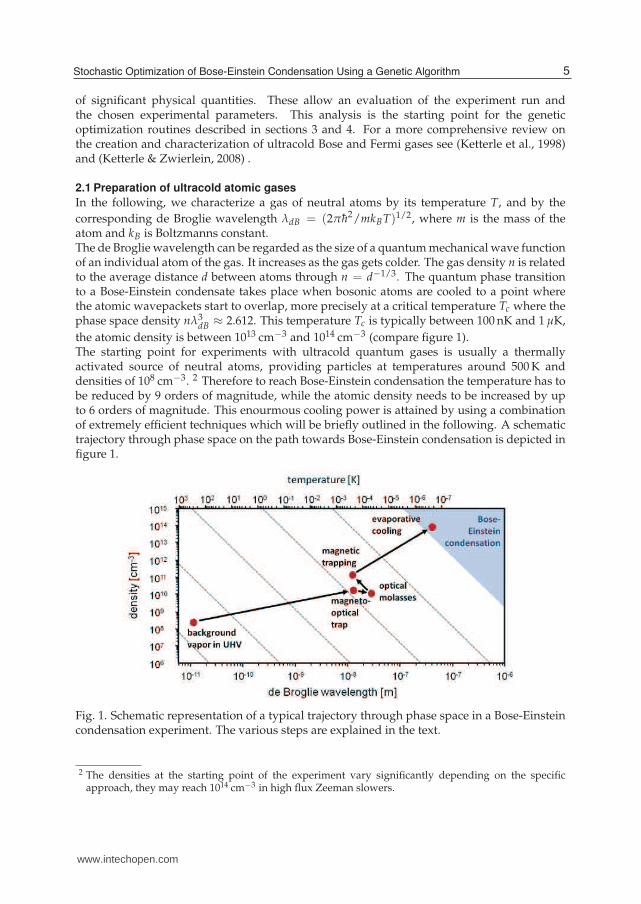
the atomic density is between 1013 cm−3 and 1014 cm−3 (compare figure 1).The starting point for experiments with ultracold quantum gases is usually a thermallyactivated source of neutral atoms, providing particles at temperatures around 500 K anddensities of 108 cm−3. 2 Therefore to reach Bose-Einstein condensation the temperature has tobe reduced by 9 orders of magnitude, while the atomic density needs to be increased by upto 6 orders of magnitude. This enourmous cooling power is attained by using a combinationof extremely efficient techniques which will be briefly outlined in the following. A schematictrajectory through phase space on the path towards Bose-Einstein condensation is depicted infigure 1.

Fig. 1. Schematic representation of a typical trajectory through phase space in a Bose-Einsteincondensation experiment. The various steps are explained in the text.

2 The densities at the starting point of the experiment vary significantly depending on the specificapproach, they may reach 1014 cm−3 in high flux Zeeman slowers.

5Stochastic Optimization of Bose-Einstein Condensation Using a Genetic Algorithm

www.intechopen.com

2.1.1 Laser cooling

Laser cooling and trapping relies on light forces, emerging when a (near-) resonant laserinteracts with atomic transitions (see (Metcalf, 1999) for a detailed description). When anatom absorbs a photon of energy hνatom, its momentum changes by hk = 2πνatom/c where kis the wave vector of the laser. When (spontaneously) emitting the photon again, the atommomentum changes again by hk. While the momentum "kick" in emission is in randomdirection and averages out over many absorption-emission cycles, the momentum transferin absorption is directive, pointing in the direction of the laser (light pressure). Hence,on average, one recoil momentum of 2πνatom/c is transferred to the atom per cycle. Theinteraction with the laser changes the momentum of an atom, which is the action of a "lightforce". This force is only determined by the frequency νatom and the scattering rate R of theatom: F = p = hkR with

R =Γ

2

s0

1 + s0 + (2Δ/Γ)2(1)

where Γ = 1/τ is the transition linewidth, s0 = I/Isat is the saturation parameter, Isat is thesaturation intensity of the atomic transition and Δ = νatom − νlaser the laser detuning withrespect to the atomic transtion frequency νatom. The maximum light force amounts to Fmax =Γhk/2 on resonance and is hence mainly determined by the linewidth of the used atomictransition. For the 780 nm D2 transition of 87Rubidium used in the experiments presentedhere, the acceleration of an atom at rest by a resonant laser is a ≈ 105 m/s2, four orders ofmagnitudes higher than gravity!Under the influence of the light force, the atom changes its velocity v quickly, giving rise to theDoppler effect. The laser now interacts with an effective detuning Δe f f = Δ+ kv. After a series

of absorption-emission cycles, (≈ 800 in the case of 87Rubidium), the effective detuning is solarge that no further interaction with the laser takes place. Turning this argument around,choosing the detuning of the laser allows to selectively address a specific velocity class ofatoms, making the light force velocity-dependent. If the laser frequency is tuned below theatomic resonance frequency νatom ("red" detuning), the laser preferably interacts with atomsmoving towards the laser, slowing them down. This method is routinely employed to slowdown atomic beams coming from a hot thermal source (Metcalf, 1999).If two counterpropagating laser beams of equal intensity and frequency are used on the atoms,the resulting light force has a dispersion-like shape. Around zero velocity, the force can beapproximated to

F = hk2 8s0Δ/Γ

(1 + (2Δ/Γ)2)2v. (2)

The light force takes the form of a friction or "molasses” force (optical molasses, see below).The cooling strength can be adjusted again by adjusting the detuning Δ. A smaller (red)detuning leads to colder temperatures. However a more narrow velocity class is thenaddressed by the laser, leading to a lower number of cooled atoms. Therefore a compromisebetween number and temperature has to be found experimentally. An optimization of lasercooling parameters using a stochastic GA can be found in section 4.The above description takes place entirely in momentum/velocity space, so far no spatialdependence and hence no trapping is introduced. To render the optical cooling force spatiallydependent, the magnetic Zeemann effect is employed. Using a quadrupole magnetic field (e.g.generated by coils in anti-Helmholtz configuration) the atomic transition is shifted, dependingon the position. With the right laser detuning (and polarization) and the right quadrupole field

6 Stochastic Optimization - Seeing the Optimal for the Uncertain

www.intechopen.com

the effective cooling force can be designed so that it points towards zero magnetic field, wherethe atoms will accumulate. The scheme can easily be extended to three dimensions, realizinga true 3d trapping of neutral atoms in free space.The combination of optical and magnetic fields to at the same time cool and spatially trapatoms is called magneto-optical-trap (MOT) and has become a standard tool in atomic physics.Its development, together with a thorough theoretical explanation of the relevant effects, ledto the award of a Nobel price in 1997 (Chu, 1998; Cohen-Tannoudji, 1998; Phillips, 1998).A MOT usually catches atoms from the low-velocity tail (≈ 10 m/s) of the thermal distributionof a background gas at room temperature or from a slowed atomic beam. Typical total atomnumbers (87Rubidium) are 108 − 109 with a density of 1011 cm−3 and a temperature of ≈200 µK. This constitutes a significant step towards Bose-Einstein condensation, as illustratedin figure 1. Almost all experiments with ultracold gases start with a phase of magneto-opticaltrapping.

2.1.2 Optical molasses

As described above, the experimental settings used in a magneto-optical trap are usuallyoptimized for trapping high number of atoms, rather than for obtaining the lowest possibletemperatures. Before loading atoms from a MOT into a conservative trapping scheme, a shortphase of "optical molasses" (1-100 ms) is employed to further lower the temperature of thegas. Here, the magnetic fields are quickly switched off, extinguishing the spatial trapping.The lasers are adjusted to different detunings (usually significantly further from the atomicresonance) and amplitudes to provide an optimal optical molasses. Atoms hence expand inthe laser field, but reduce their kinetic energy (and hence the temperature of the sample, oncerecaptured in a conservative trap). As the atoms fulfill a damped Brownian motion, they willultimately diffuse out of the volume that can be captured by a conservative trap. Again acompromise has to be found between temperature (favoring long molasses times) and atomnumber (favoring short molasses times) to be transferred.Several different processes contribute to the enhanced cooling in the optical molasses, such asSisyphus cooling or dark state effects which go beyond the simple model of Doppler coolingdescribed above. For a comprehensive overview see (Metcalf, 1999).

2.1.3 Conservative atom trapping

Even though laser cooling and optical molasses allow an enormous gain in phase spacedensity, there are fundamental limits. As all optical forces rely on absorption and successiveemission of photons, the random momentum transfer in spontaneous emission induces aheating mechanism which limits the temperatures that can be achieved. A lower bound,termed the recoil limit, can be obtained by calculating the energy associated with a singlephoton recoil:

Erecoil = kBTrecoil =h2k2

2m. (3)

For 87Rubidium atoms and the standard 780 nm D2 transition, this corresponds to atemperature of 0.4 µK.Therefore to confine and further cool the gas, another trapping scheme has to be employedwhich does not rely on photon exchange. Such traps can be constructed using the interactionof an electric3 or magnetic dipole moment with external electric or magnetic fields. These

3 Note that most experiments with ultracold atoms are performed with alkali atoms, where the electricdipole moment is only induced in the presence of en external electric field.

7Stochastic Optimization of Bose-Einstein Condensation Using a Genetic Algorithm

www.intechopen.com

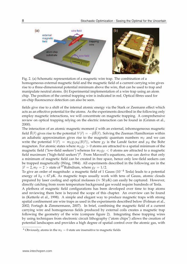
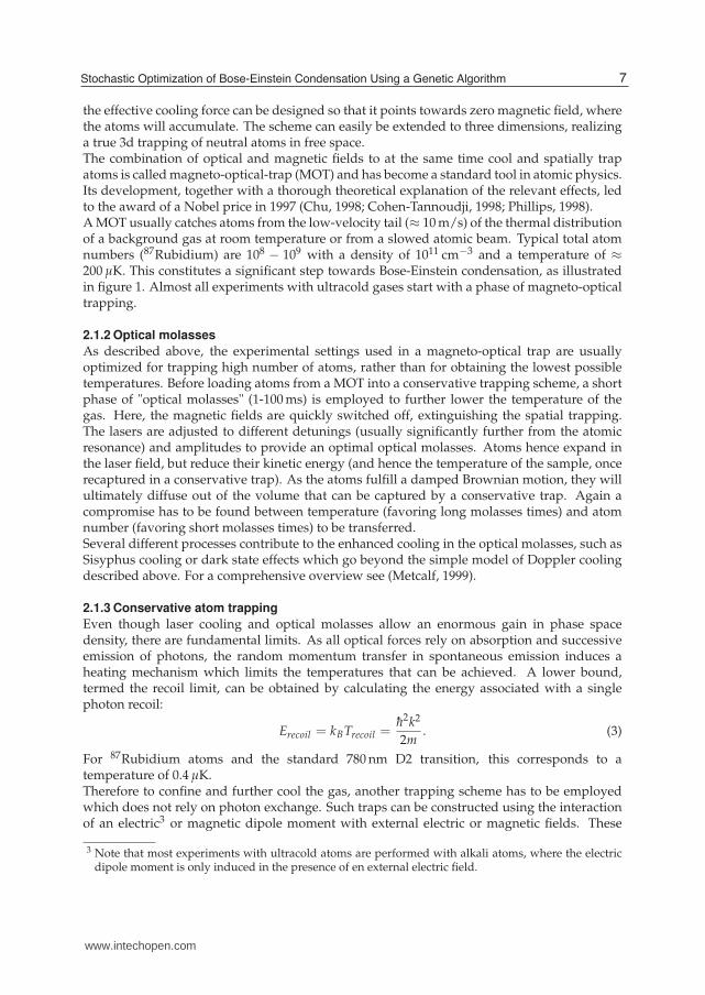
Fig. 2. (a) Schematic representation of a magnetic wire trap. The combination of ahomogeneous external magnetic field and the magnetic field of a current carrying wire givesrise to a three-dimensional potential minimum above the wire, that can be used to trap andmanipulate neutral atoms. (b) Experimental implementation of a wire trap using an atomchip. The position of the central trapping wire is indicated in red. Optical fibres used foron-chip fluorescence detection can also be seen.

fields give rise to a shift of the internal atomic energy via the Stark or Zeemann effect whichacts as an effective potential for the atoms. As the experiments described in the following onlyemploy magnetic interactions, we will concentrate on magnetic trapping. A comprehensivereview on optical trapping relying on the electric interaction can be found in (Grimm et al.,2000).The interaction of an atomic magnetic moment �µ with an external, inhomogeneous magnetic

field �B(�r) gives rise to the potential V(�r) = −�µ�B(�r). Solving the Zeeman Hamiltonian withinan adiabatic approximation gives rise to the magnetic quantum numbers mF and we canwrite the potential V(�r) = mFgFµB|B(�r)|, where gF is the Landé factor and µB the Bohrmagneton. For atomic states where mFgF > 0 atoms are attracted to a spatial minimum of themagnetic field ("low-field seekers") whereas for mFgF < 0 atoms are attracted to a magneticfield maximum ("high-field seekers")4. From Maxwell’s equations, one can derive that onlya minimum of magnetic field can be created in free space, hence only low-field seekers canbe trapped magnetically (Wing, 1984). All experiments described in the following are in the|F = 2, mF = 2 > state of 87Rubidium, where gF = 1/2.To give an order of magnitude: a magnetic field of 1 Gauss (10−4 Tesla) leads to a potentialenergy of kB × 67 µK. As magnetic traps usually work with tens of Gauss, atomic cloudsprepared by laser cooling and optical molasses (≈ 50 µK) can easily be captured. However,directly catching from room temperature background gas would require hundreds of Tesla.A plethora of magnetic field configurations has been developed over time to trap atomsand reviewing them here is beyond the scope of this chapter. An overview can be foundin (Ketterle et al., 1998). A simple and elegant way to produce magnetic traps with strongspatial confinement are wire traps as used in the experiments described below (Folman et al.,2002; Fortagh & Zimmermann, 2007). In brief, combining the magnetic field of a currentcarrying wire and homogeneous fields produced by external coils creates a magnetic trapfollowing the geometry of the wire (compare figure 2). Integrating these trapping wiresby using techniques from electronic circuit lithography ("atom chips") allows the creation ofpotential landscapes and provides a high degree of spatial control over the atomic gas, with

4 Obviously, atoms in the mF = 0 state are insensitive to magnetic fields

8 Stochastic Optimization - Seeing the Optimal for the Uncertain

www.intechopen.com

high temporal resolution. Bose-Einstein condensation on a chip was first demonstrated in2001 (Hänsel et al., 2001; Ott et al., 2001; Schneider et al., 2003), and atom chips have sincethen become a standard tool in ultracold atom research.

2.1.4 Evaporative cooling

Magnetic trapping as described above provides a means to confine neutral atoms of aspecific temperature in free space. However, as magnetic (and also electric) potentialsare conservative, no cooling takes place. The temperature of the gas can be changed by(adiabatically) changing the atomic confinement, however, phase space density is maintainedand hence no progress towards Bose-Einstein condensation can be made.

Fig. 3. (a) Principle of evaporative cooling. A thermal Maxwell-Boltzmann distributioncharacterized by a temperature Ti is truncated at energy Etrunc with Etrunc > kBTi. Thetruncated system relaxes to thermal equilibrium at a lower temperature Tf . (b) Selectiveremoval of hot atoms by adjusting the frequency ωRF driving spin flip transitions tountrapped states.

To gain in phase space density and decrease the gas temperature in a steady trap, an additionalcooling mechanism termed "evaporative cooling" is employed. Similar to blowing onto acoffee cup, evaporative cooling relies on the selective removal of energetic (hot) particles. Thesystem successively relaxes back to thermodynamic equilibrium (via particle collisions) at alower temperature (see figure 3).To selectively remove hot atoms from the magnetic trap, spin-flip transitions between trappedand untrapped Zeeman states are induced using radio frequency (RF) fields. By choosing theRF-field’s frequency, the transitions occur at distinct regions in space (magnetic equipotentialsurfaces). The "hottest" atoms with highest kinetic energy explore the outwardmost regionsof the magnetic trap, so these can be removed selectively ("RF knife"). As the systemre-thermalizes at lower temperature, the frequency of the RF field has to be adjusted. Thisleads to dynamic forced evaporative cooling with time (Davis et al., 1995b; Luiten et al., 1996).As illustrated in figure 1, evaporative cooling allows to reduce the temperature of agas by another two orders of magnitude and has enabled the creation of Bose-Einsteincondensates (Davis et al., 1995a). However, the atom number is reduced by a similar factor.So far, no cooling method able to achieve such low temperatures while maintaining theinitial atom number has been found. The details of the evaporative cooling process cruciallydepend on the details of the experimental implementation, in particular on the lifetime of

9Stochastic Optimization of Bose-Einstein Condensation Using a Genetic Algorithm

www.intechopen.com

the magnetically trapped atoms and the collision and hence re-thermalization rate. Theoptimization of evaporative cooling using a stochastic GA is described in section 4.

2.2 Detection

Most information in ultracold atom experiments is gained through the interaction of atomswith light. Although several non-optical methods for specific applications or unique atomspecies (Santos et al., 2002) are in use, optical imaging is currently the main detection methodfor cold atomic gases. As far as imaging is concerned, atom-light interactions can be dividedinto three processes: absorption, re-emission and phase alteration of incident light, givingrise to three detection methods, two of which - absorption and fluorescence imaging - areused in our experiment5. Both methods result in a picture of the atom cloud, destroyingit in the process. Quantities characterizing the state of the cloud can be extracted eitherfrom a single picture or from a series of images taken while varying one of the experimentalparameters from shot to shot. The following section will describe these quantities and how tomeasure them. Suitable light sources for excitation of atoms are lasers tunable in the frequencyrange near an atomic transition, while CCD - cameras are ideal detectors for light (or lackthereof) whenever time resolution is not a critical factor.6 In order to reach the resolutionsneeded for the examination of structures like interference fringes or vortices inside cold atomicclouds, it is neccessary to put special emphasis on the imaging optics, which usually has to becustom-built for each experiment.

2.2.1 Absorption imaging

This method consists in recording the shadow which an atom cloud casts onto a detectordue to the absorption of a certain fraction of photons when irradiated with laser light. Bycomparison with the intensity of the beam in absence of the atomic cloud, the atoms’ densitydistribution and a series of other parameters discussed in section 2.2.3 can be calculated. Thedetection beam can be absorbed almost completely if the density of the atom cloud becomessufficiently high. These optically dense clouds make a quantitative analysis of an absorptionimage difficult. In order to compensate for this, it is possible to detune the laser light fromresonance, lowering the absorption cross-section. The former introduces diffraction as well asa phase shift of the transmitted light, and going to high detunings as well as filtering out theunscattered transmitted light components leads to dispersive imaging. Absorption imagingintroduces heating: Since each absorbed photon transfers a momentum hk to the atom, thecloud is literally blown away by the imaging light, making absorption imaging a destructivetechnique.

2.2.2 Fluorescence imaging

In fluorescence imaging, the atom cloud is also irradiated with a laser beam. However now itis not the transmitted intensity that is measured, but the number of photons scattered into thesolid angle Ω covered by the detector. If Ω were equal to 4π, fluorescence imaging would justcollect all the photons missing from an absorption picture. However, since the detector usually

has a coverage factor fc =Ω4π of a few percent, in comparison the fluorescence signal is about

a factor 100 weaker. Yet, fluorescence imaging has two advantages: In situations where the

5 For a review of dispersive imaging methods, see for example (Ketterle et al., 1998) and referencestherein.

6 For fast detection, photomultipliers or avalanche photodiodes are required, trading their advantagesfor lower detection efficiency and, in most cases, lower spatial resolution.

10 Stochastic Optimization - Seeing the Optimal for the Uncertain

www.intechopen.com

dissipative light force is used to trap the atoms - the MOT and optical molasses phase in ourexperiment - fluorescence photons come “for free” and allow non-destructive measurements.Additionally, fluorescence imaging has favourable properties for imaging dilute atom clouds.A comparison of the signal to noise ratio (SNR) - neglecting all noise sources except atomicshot noise - for absorption and fluorescence imaging yields:

SNR f

SNRa=

√

fc

OD. (4)

Thus, if the cloud’s optical density OD drops below the coverage factor, fluorescence imagingbecomes better in terms of SNR, at least as long as other noise sources deliver a comparablecontribution for both methods. Hence, fluorescence imaging is the preferred technique fordetecting extremely dilute clouds. In contrast to absorption imaging, fluorescence detectorsneed not be exposed to the high light intensities of the source laser illuminating the atoms. Asa consequence, highly sensitive detectors like EMCCD cameras and avalanche photodiode- based single photon counting modules can be employed. Several techniques based onfluorescence, like lightsheet imaging (Bücker et al., 2009; Rottmann, 2006) or fiber-baseddetection methods allow to detect atomic clouds with single atom sensitivity.

2.2.3 Evaluating absorption images

The intensity of a monochromatic light beam travelling in y - direction through an opaquemedium is attenuated with

dI

dy= −σIn (5)

where σ denotes the scattering cross-section and n the density of the atomic cloud. As long asthe cross-section is a constant with respect to intensity, i.e. in the case of linear optics definedby low intensities7, this equation can simply be integrated to yield Lambert - Beer’s law as result:

I = I0e−σn. (6)

If we allow a density distribution in the (x, z) direction, this gives I(x, z) = I0(x, z)e−σnc(x,z),with column density nc(x, z) =

∫

dy n(x, y, z). The scattering cross-section depends on the

detuning Δ, with σ(Δ) = σ0/(

1 + (2Δ/Γ)2)

. The column density can then be expressed as:

nc(x, z) = σ(Δ) ln

(

I0(x, z)

It(x, z)

)

. (7)

This measured column density allows to deduce important basic properties of the diluteatomic cloud:

• Total atom numberIn the continuous case, the total atom number can be obtained by integrating the columndensity:

N =∫

nc(x, z) dx dz. (8)

In the experiment, we have to consider that x and z are discrete, their step size definedby the area A imaged onto a single CCD pixel, with the magnification M. Therefore, for

7 For high intensities, stimulated emission begins to play a role, leading to an enhanced forwardscattering rate

11Stochastic Optimization of Bose-Einstein Condensation Using a Genetic Algorithm

www.intechopen.com

a square region of interest containing p pixels, equation 8 becomes the discrete sum overthese pixels:

N = A ∑p

np(x, y) =ΔxPixelΔyPixel

M2 ∑p

np(x, y). (9)

• Thermal Atom Density in the Trap

In order to derive temperature or temperature-dependent quantities like phase spacedensity, or to gain information about the trapping potential, we need a model whichdescribes the density distribution of the atoms in the trap, as well as its evolutionafter releasing the cloud from the trap. Since thermal atom clouds and Bose - Einsteincondensates represent different thermodynamic phases, where density is closely linked tothe phase transition’s order parameter, one expects different behaviour in the two regimes.

Trapping potentials created by static magnetic fields are harmonic around the fieldminimum:

V(x, y, z) =m

2

(

ω2xx2 + ω2

yy2 + ω2z z2

)

. (10)

For a thermal cloud of bosons, the density distribution for high temperatures can beexpressed as (Ketterle et al., 1998; Reichl, 1998)

n(r) =

(

2πh2

mkBT

)3/2

g3/2 (z (r)) (11)

with z = e(µ−V(x,y,z))/kBT . Here, gj(z) = ∑izi

ij is the Bose function, introducing Boseenhancement, which means increased density compared to the classical case, where thedistribution would be Gaussian. For high temperatures or low densities, we can neglect

Bose enhancement, and with the halfwidths wi =

√

2kBTmω2

i

, i = x, y, z and zero chemical

potential, we recover a Gaussian distribution:

n(x, y, z) = n0e−(

x2

w2x+ y2

w2y+ z2

w2z

)

. (12)

Experimentally, we only have access to column densities:

nc(x, z) =∫

dy n(x, y, z) = n0

√πwye

−(

x2

w2x+ z2

w2z

)

= n0e−(

x2

w2x+ z2

w2z

)

. (13)

We can determine n0 by normalization with respect to the atom number:

N =∫

dx dz nc(x, z) ⇒ n0 =N

πwxwz. (14)

By comparison with equation 13 we can calculate the peak density of the thermal cloud:

n0 =n0√πwy

. (15)

12 Stochastic Optimization - Seeing the Optimal for the Uncertain

www.intechopen.com

Equivalently, n0 can be determined directly from normalization of equation 12. Since thepicture is integrated along y, we need an assumption about the density distribution on thisaxis. Our magnetic traps yield cigar-shaped atom clouds, therefore it usually holds thatwy = wz.

• TemperatureA thermal atom cloud released from a trap by suddenly (non-adiabatically) switchingoff the trapping potential expands isotropically, the intitial isotropic velocity distributionbeing conserved. The evolution of the cloud’s half-width is given by

wri (t)2 =

2kBT

mω2i

+2kBT

mt2. (16)

By repeatedly measuring w2ri

at different times of flight t2 and plotting the two quantities

against each other, the temperature can be determined by the resulting line’s slope 2kBT2

m .For t = 0, an estimation of the trap frequency in direction ri is possible.

• Phase Space DensityThe important quantity which has to reach a treshold value of 2.612 in order to achieveBose–Einstein condensation is the phase space density of the atomic cloud:

D = n0 λ3dB (17)

comprising the peak density n0 and the thermal de Broglie wavelength λdB =√

2πh2

mkBT .

3. Stochastic optimization in an ultracold atom experiment

3.1 Setup of the feedback loop

The goal of our experiment is the investigation of ultracold 87Rubidium clouds in chip - basedmagnetic traps, employing all steps involving preparation, manipulation and detection of theatoms described in the previous sections. The focus lies on the application of fiber opticsintegrated directly on the chip as a tool for the detection of ultracold atoms (Heine et al.,2010).Figure 4 illustrates our hardware feedback loop. A real-time control system governs thebehavior of the experimental apparatus via 30 output channels providing analog controlvoltage signals, as well as 28 digital TTL channels, with a time resolution of 25 µs. Thecontrol channels allow us to manipulate practically all aformentioned experimental quantities,including laser detunings and intensities, magnetic field strengths and radio frequency fields,both in timing and magnitude. User input is collected by an interface software written inMATLAB.Our absorption images of atomic clouds are taken with a Pixelfly QE interline CCDcamera, read out and evaluated by a MATLAB program on a dedicated computer. Thealgorithm providing feedback between acquisition and control software is also implementedin MATLAB as part of the acquisition software, and communication between acquisition andcontrol hardware is established via a UDP interface provided by MATLAB.Briefly, our experimental sequence consists of a magneto-optical trap followed by a molassesstage. The atoms are then loaded into a magnetic trap created using a macroscopicwire structure located behind the atom chip, and subsequently cooled using RF-inducedevaporation. All data discussed in section 4 was obtained by absorption imaging of atomic

13Stochastic Optimization of Bose-Einstein Condensation Using a Genetic Algorithm

www.intechopen.com

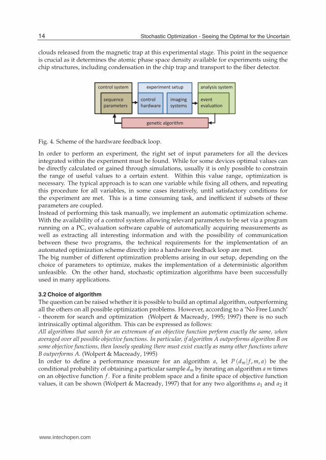
clouds released from the magnetic trap at this experimental stage. This point in the sequenceis crucial as it determines the atomic phase space density available for experiments using thechip structures, including condensation in the chip trap and transport to the fiber detector.

control system experiment setup analysis system

sequence

parameters

control

hardware

imaging

systems

event

evaluaピﾗﾐ

geneピI algorithm

Fig. 4. Scheme of the hardware feedback loop.

In order to perform an experiment, the right set of input parameters for all the devicesintegrated within the experiment must be found. While for some devices optimal values canbe directly calculated or gained through simulations, usually it is only possible to constrainthe range of useful values to a certain extent. Within this value range, optimization isnecessary. The typical approach is to scan one variable while fixing all others, and repeatingthis procedure for all variables, in some cases iteratively, until satisfactory conditions forthe experiment are met. This is a time consuming task, and inefficient if subsets of theseparameters are coupled.Instead of performing this task manually, we implement an automatic optimization scheme.With the availability of a control system allowing relevant parameters to be set via a programrunning on a PC, evaluation software capable of automatically acquiring measurements aswell as extracting all interesting information and with the possibility of communicationbetween these two programs, the technical requirements for the implementation of anautomated optimization scheme directly into a hardware feedback loop are met.The big number of different optimization problems arising in our setup, depending on thechoice of parameters to optimize, makes the implementation of a deterministic algorithmunfeasible. On the other hand, stochastic optimization algorithms have been successfullyused in many applications.

3.2 Choice of algorithm

The question can be raised whether it is possible to build an optimal algorithm, outperformingall the others on all possible optimization problems. However, according to a ’No Free Lunch’- theorem for search and optimization (Wolpert & Macready, 1995; 1997) there is no suchintrinsically optimal algorithm. This can be expressed as follows:All algorithms that search for an extremum of an objective function perform exactly the same, whenaveraged over all possible objective functions. In particular, if algorithm A outperforms algorithm B onsome objective functions, then loosely speaking there must exist exactly as many other functions whereB outperforms A. (Wolpert & Macready, 1995)In order to define a performance measure for an algorithm a, let P (dm| f , m, a) be theconditional probability of obtaining a particular sample dm by iterating an algorithm a m timeson an objective function f . For a finite problem space and a finite space of objective functionvalues, it can be shown (Wolpert & Macready, 1997) that for any two algorithms a1 and a2 it

14 Stochastic Optimization - Seeing the Optimal for the Uncertain

www.intechopen.com

applies that

∑f

P (dm| f , m, a1) = ∑f

P (dm| f , m, a2) . (18)

Therefore in order to deliver optimal performance, optimization algorithms have to bematched or tailored to specific problems. The main point in this context is the balancebetween what is called ’exploration versus exploitation’. Any random search mechanismswithin an algorithm contribute to exploration, while gradient search - based elements exploitthe parameter space structure in order to find the optimum. As a consequence, picking analgorithm and choosing its parameters to fit the problem at hand is as valid an approach aschoosing a specific algorithm.Out of the many different methods available, we choose to implement a real coded geneticalgorithm (RCGA). Belonging to the first stochastic optimization methods developed, theconvergence behavior of genetic algorithms is well documented for different classes ofproblem spaces. They belong to the class of global optimization algorithms, exploitinginformation from different parts of the problem space in parallel as opposed to localalgorithms like e.g. stochastic hill climbing or simulated annealing. This property reducesthe probability of premature convergence towards local optima. RCGAs allow to definestates directly from real valued optimization parameters, without any intermediate encoding,which is simple and intuitive. While early literature suggests that binary encoding is keyto the convergence properties of genetic algorithms, more recent studies, backed up by anincreasing number of applications, have shown that real coded algorithms suffer from nogeneral disadvantages as compared to other encoding schemes, and even perform better formany applications.

3.3 Implementation

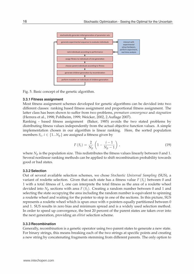
The basic concept of the algorithm, as depicted in figure 5, is the same as applies to theinitial canonical genetic algorithm and most subsequent implementations. After generationof a random starting population of states, real valued parameter vectors, the experiment isperformed and evaluated for each state with respect to a measured value representing theobjective function of the optimization problem. Based on the measurement results, the statesare ranked and fitness values are assigned accordingly. The fitness values determine theprobability for each state to be selected as a parent for a recombination procedure providingthe next generation of states. After recombination, each state undergoes mutation, a stochasticalteration of one of its parameter values, with a preset probability. Subsequently, the nextiteration begins by evaluating the resulting parameter vectors by experiment.The time consuming process in this setup is evaluating the objective function, which meansperforming the experiment, with a duration of 35 seconds. Even more so than in purelycomputational applications of GAs, it is crucial to minimize the number of iterations beforefinding the optimum. Since runtime crucially depends on the number of states within eachgeneration, the population size, the design goal is to keep this number as low as possiblewhile preventing premature convergence due to rapidly decreasing diversity of the states.Simulations, backed up by our experiments, indicate that with proper adjustment of thegenetic operators, as described in the next section, a population size of 20 states can ensurereliable convergence behavior for realistic problem spaces.

15Stochastic Optimization of Bose-Einstein Condensation Using a Genetic Algorithm

www.intechopen.com

stochasピcally generate iniピal generaピon of parameter sets

generate experimental sequence to evaluate individuals

rank individuals according to performance

assign gtness to individuals of one generaピon

choose parent individuals according to gtness

generate children generaピon by recombinaピon

perform mutaピon on individuals of children generaピon

interact with

experimental

setup hardware,

perform experiment,

real ピme analysis

Fig. 5. Basic concept of the genetic algorithm.

3.3.1 Fitness assignment

Most fitness assignment schemes developed for genetic algorithms can be devided into twodifferent classes: ranking based fitness assignment and proportional fitness assignment. Thelatter class has been shown to suffer from two problems, premature convergence and stagnation(Herrera et al., 1998; Pohlheim, 1999; Weicker, 2002, 2.Auflage 2007).Ranking - based fitness assignment (Baker, 1985) avoids the two stated problems bydistributing fitness values independently from the actual objective function values. A simpleimplementation chosen in our algorithm is linear ranking. Here, the sorted populationmembers Si, i ∈ {1...Np} are assigned a fittness given by

F (Si) =2

Np

(

1 − i − 1

Np − 1

)

, (19)

where Np is the population size. This redistributes the fitness values linearly between 0 and 1.Several nonlinear ranking methods can be applied to shift recombination probability towardsgood or bad states.

3.3.2 Selection

Out of several available selection schemes, we chose Stochastic Universal Sampling (SUS), avariant of roulette selection. Given that each state has a fitness value F (Si) between 0 and1 with a total fitness of 1, one can interprete the total fitness as the area of a roulette wheeldevided into Np sections with area F (Si). Creating a random number between 0 and 1 andselecting the state occupying the area including the random number is equivalent to spinninga roulette wheel and waiting for the pointer to stop in one of the sections. In this picture, SUSrepresents a roulette wheel which is spun once with n pointers equally partitioned between 0and 1. SUS results in zero bias and minimum spread and is a widely used selection method.In order to speed up convergence, the best 20 percent of the parent states are taken over intothe next generation, providing an elitist selection scheme.

3.3.3 Recombination

Generally, recombination is a genetic operator using two parent states to generate a new state.For binary strings, this means breaking each of the two strings at specific points and creatinga new string by concatenating fragments stemming from different parents. The only option to

16 Stochastic Optimization - Seeing the Optimal for the Uncertain

www.intechopen.com

vary in this case is the number of fragments the parents are broken in, leading to single-point,multi-point or uniform crossover. The latter represents simply an extreme case of multi-pointcrossover, where the m - bit parent states are decomposed into n fragments.For RCGAs, the state is represented by a string or vector of real numbers. Translating theidea of crossover to this situation gives what is called discrete recombination. One methodto implement this is to decide for each vector component vj of the child state SC

i (vj) whichparent (P1 or P2) contributes the variable value:

vCj = vP1

j aj + vP2

j

(

1 − aj

)

. (20)

Here, aj is randomly chosen to be 0 or 1 for each vCj separately and j ∈ {1, ..., m}, where m

denotes the total number of variables.With discrete recombination, only variable values already realized in the starting populationcan be reached. In order to gain access to new value regions, real number representedstates allow interpolation between two values. The most general recombination scheme tobe derived this way is intermediary recombination. It can be implemented with equation 20,but an aj picked from the interval [−d, 1 + d] with uniformly distributed probability for eachvariable separately. This operator is also called BLX - α (blend crossover), where α equals 2d.The hypercuboid of possible new values has a volume of

VCPS = (1 + 2d)

m

∏j=1

lj (21)

with lj as length of the value region spanned by the variables vP1,P2j and a total of m variables.

For d = 0, the hypercuboid containing the possible children values is as big as the one spannedby the parent variables. Since the probability for a child value to lie inside the cuboid is higherthan the probability to lie on its bounds, the cuboid volume will decrease with a growingnumber of iterations in this case, restricting the accessible part of the problem space withoutany influence of selection. By stretching the children’s value space by the factor (1 + 2d)one can compensate for this effect. Empirically, a value of d = 0.25 (BLX-0.5) has proven toconserve the cuboid volume in the limit of a large iteration number.If aj is not chosen for each variable separately, but rather once in the beginning of therecombination phase and kept the same for all variables, the linear recombination can berecovered as special case of intermediary recombination.Since intermediary recombination with d = 0.25 (BLX-0.5) gives optimal convergencebehaviour in many computer experiments Herrera et al. (1998); Pohlheim (1999), it has beenchosen for our algorithm. Since it delivers real numbers as variable values while our stepsizesimposes a whole number representation, the routine’s results are rounded to match the nearestallowed variable value.

3.3.4 Mutation

Mutation in an RGCA means randomly changing values in the state vector. A commonlyused mutation routine has been presented in Mühlenbein & Schlierkamp-Voosen (1993) andMühlenbein & Schlierkamp-Voosen (1995), and can be described as follows:

vmutj = vj + sj · rDj · 2−uκm . (22)

17Stochastic Optimization of Bose-Einstein Condensation Using a Genetic Algorithm

www.intechopen.com

Here, vmutj and vj denote the mutated and source states respectively, while sj randomly

chooses the sign of the mutation step, r defines the mutation range as fraction of the variabledefinition domain Dj. The last term designates the used distribution characterized by therandom number u which is uniformly distributed in the interval [−1, 1] and the mutation

precision κm. The latter defines a lower limit of 12−κm

for the mutation step size. Favoringsmall mutation steps over big ones, nonuniform mutation operators like this have shown tobe advantageous for RCGAs in computer experiments.From runs on test problems, our algorithm with population sizes between 20 and 30 hasgiven good results with κm = 10, r = 0.2 and an overall mutation rate of 10 percent. Thisis consistent with literature suggesting that optimal mutation rates are inversely proportionalto population size Haupt (2000).

4. Examples of stochastic optimization

4.1 Optimization of an optical molasses

The measurement presented here allows a simple comparison of a grid scan to thegenetic-algorithm approach. The optical molasses has already been briefly described insection 2.1.2. In this phase, it is possible to reduce the temperature of 87Rubidium atomsfrom the magneto-optical trap by an order of magnitude to ensure that a large fraction of thecloud has low enough energy to be trapped in a conservative magnetic trapping potential.This phase relies purely on the interaction of atoms with laser light. In our measurement,the optimized quantity is the atom number within the magnetic trap after the molassesphase, and the optimized parameters are molasses duration and laser detuning. Variationsin the experimental conditions due for example to environmental noise, lead to a statisticaluncertainty in the measured value. We therefore average over multiple experimental runs toreduce this uncertainty. The successful optimization of this experimental stage is shown infigure 6. In the 2d grid scan, we changed the detuning in steps of 5 MHz and the molassesduration in steps of 0.2 ms, and computed the average of 4 atom-number measurements ateach pair of values, resulting in a scan duration of approximately 17 hours. For the GAoptimization, we used a population size of 20 states and recorded the convergence over16 generations. In this case, we only averaged over 3 atom number measurements. Thisoptimization approach led to a reduction of the runtime to approximately 9 hours. The set ofsurviving parameters has already clustered near the optimum after this time, demonstratingthe efficiency of the approach.

4.2 Optimization of evaporative cooling in a magnetic trap

The goal of evaporative cooling in a magnetic trap is to increase phase space density (seesections 2.1.4 and 2.2) of the atomic cloud as efficiently as possible. Efficiency meansmaximizing the amount of removed energy per removed atom. Technically, evaporativecooling as described in 2.1.4 is implemented with the help of an RF source that is tunable infrequency and therefore can create RF - cooling ramps by lowering the frequency of the appliedfield on timescales ranging from milliseconds to seconds. Frequencies from 10 MHz down tothe 100 kHz range with sub - kHz stability and corresponding resolution have to be provided.In an ideal system, efficiency grows with ramp duration. The slower the ramp, the more timethe system has to stochastically produce atoms with high energy that are removed by the RFfield, while fast cooling means removing more atoms with lower energy. In reality, constraintsfor the steepness of these ramps are imposed mainly by two mechanisms: On the one hand,

18 Stochastic Optimization - Seeing the Optimal for the Uncertain

www.intechopen.com

0 5 10 15 20−5

0

5

10

15x 10

6

Generation

Obje

ctive F

unction V

alu

e

Mean fitness per generation

(a)

0 50 100 150 200 250−100

−80

−60

−40

−20

0

20

40

State

Para

mete

r V

alu

es

State Evolution

(b)

Detuning (MHz)

Mo

lass

es

Du

rati

on

(m

s)

−65 −60 −55 −50 −45 −40 −35 −30 −25 −20 −15 −10

11

12

13

14

15

16

17

(c)

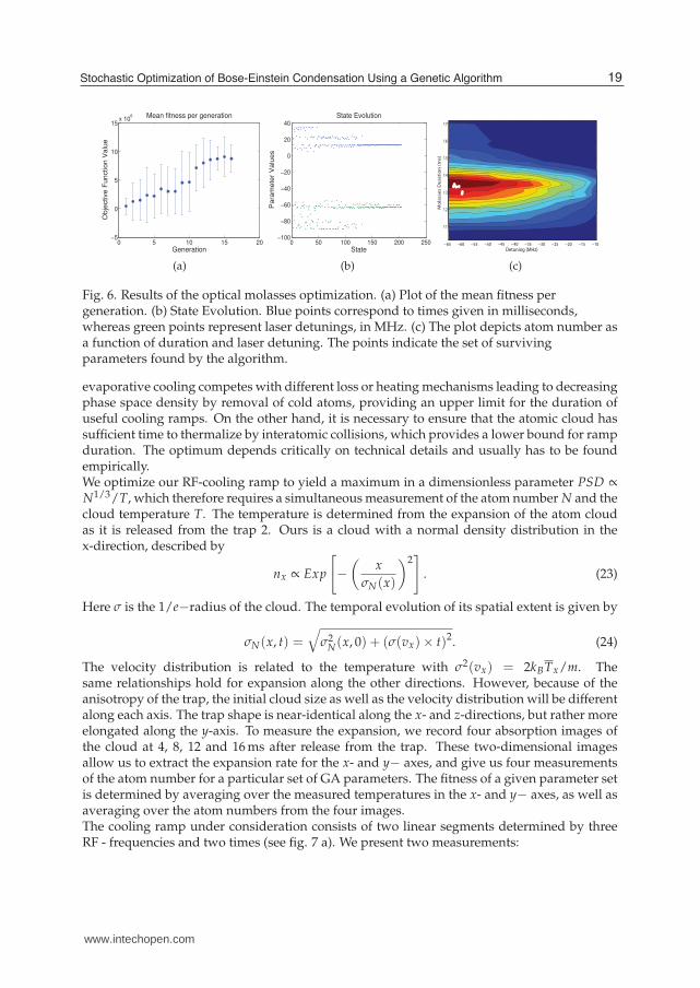
Fig. 6. Results of the optical molasses optimization. (a) Plot of the mean fitness pergeneration. (b) State Evolution. Blue points correspond to times given in milliseconds,whereas green points represent laser detunings, in MHz. (c) The plot depicts atom number asa function of duration and laser detuning. The points indicate the set of survivingparameters found by the algorithm.

evaporative cooling competes with different loss or heating mechanisms leading to decreasingphase space density by removal of cold atoms, providing an upper limit for the duration ofuseful cooling ramps. On the other hand, it is necessary to ensure that the atomic cloud hassufficient time to thermalize by interatomic collisions, which provides a lower bound for rampduration. The optimum depends critically on technical details and usually has to be foundempirically.We optimize our RF-cooling ramp to yield a maximum in a dimensionless parameter PSD ∝

N1/3/T, which therefore requires a simultaneous measurement of the atom number N and thecloud temperature T. The temperature is determined from the expansion of the atom cloudas it is released from the trap 2. Ours is a cloud with a normal density distribution in thex-direction, described by

nx ∝ Exp

[

−(

x

σN(x)

)2]

. (23)

Here σ is the 1/e−radius of the cloud. The temporal evolution of its spatial extent is given by

σN(x, t) =√

σ2N(x, 0) + (σ(vx)× t)2. (24)

The velocity distribution is related to the temperature with σ2(vx) = 2kBTx/m. Thesame relationships hold for expansion along the other directions. However, because of theanisotropy of the trap, the initial cloud size as well as the velocity distribution will be differentalong each axis. The trap shape is near-identical along the x- and z-directions, but rather moreelongated along the y-axis. To measure the expansion, we record four absorption images ofthe cloud at 4, 8, 12 and 16 ms after release from the trap. These two-dimensional imagesallow us to extract the expansion rate for the x- and y− axes, and give us four measurementsof the atom number for a particular set of GA parameters. The fitness of a given parameter setis determined by averaging over the measured temperatures in the x- and y− axes, as well asaveraging over the atom numbers from the four images.The cooling ramp under consideration consists of two linear segments determined by threeRF - frequencies and two times (see fig. 7 a). We present two measurements:

19Stochastic Optimization of Bose-Einstein Condensation Using a Genetic Algorithm

www.intechopen.com

Time

RF

freq

uen

cy

Duration 1

Duration 2

Fre

qu

en

cy 1

Freq

ue

ncy 2

(a)

0 4 8 12 16

0

100

200

300

400

t �ms�

ΣN�Μm�

(b)

Fig. 7. Example of data for one population member. a) Schematic of an RF - ramp, depictingthe used optimization parameters. Arrows indicate the RF frequencies modified in the 2d -optimization run. In the 4d scan, the cooling ramp was optimized over the rectangular areasspanning duration and frequency of the two stages. b) Fits to equation (24) for the x- and y−axes in red and blue, respectively. The inset panels show absorption images of the atomcloud as it falls and expands after release from the magnetic trap, at the corresponding times.Each panel shows a region of approximately 1.5 mm× 1.8 mm.

• A 2d measurement, where the algorithm adjusts the intermediate and final value of the RFfrequency. The values ranges from 0 to 10 and 0 to 1 MHz, respectively.

• A 4d measurement, where the algorithm adjusts both field values from the 2dmeasurement as well as both times. RF values range from 2 to 6 and 0.3 to 0.6 MHzrespectively, in steps of 0.01 MHz. The times for the first and second ramp segment cantake values each from 500 to 2000 ms (duration 1) and 500 to 3500 ms (duration 2), in stepsof 1 ms.

The results are summarized in figure 8. Unlike the molasses optimization described above, wehave not compared this measurement to a grid scan. In the case of the 4d-optimization this issimply not feasible, given that the explored parameter space contains of over 1011 individualpoints corresponding to over 10000 years of experiment runtime. Even by reducing the timeresolution to 10 ms as well and changing the frequency steps to 0.05 MHz, the measurementduration remains large, at roughly 50 years. Unless an optimization approach like ours isimplemented, only physical arguments and a certain degree of parameter separability can beused to find useful working points for ramp parameters for this and similar problems, leadingto a labor-intensive manual search.For the 2d measurement, the algorithm finds values of 3 MHz and 0.65 MHz for the RF- ramp frequencies. Although we cannot make a quantitative statement about the qualityof this solution without knowledge of the parameter space, these values are similar to thecooling ramp values which have been successfully used before GA - optimization as well asthe corresponding phase space densities. Note that the algorithm has not fully converged forthe intermediate RF value; a competing subpopulation with 2 MHz RF - value is still presentin the last generation.For the 4d measurement, the algorithm also finds an intermediate value of 3 MHz, but a lowerend frequency of 0.47 MHz. Objective function values, especially those of the best performingstates within the run, are only slightly inferior to those in the last generations of the 2dmeasurement. It is interesting to see however that performance increases towards the endof the run, at the same time when the competing subpopulation for short times of duration 1

20 Stochastic Optimization - Seeing the Optimal for the Uncertain

www.intechopen.com

0 100 200 300 4000

2

4

6

8

10

State

Para

mete

r V

alu

es

State Evolution

(a) 2d optimization run.

0 100 200 300 400 5000

1

2

3

4

5

6

State

Pa

ram

ete

r V

alu

es

State Evolution

(b) 4d optimization run I.

0 100 200 300 400 500500

1000

1500

2000

2500

3000

3500

State

Para

mete

r V

alu

es

State Evolution

(c) 4d optimization run II.

0 5 10 15 20−1

0

1

2

3

4

5

Generation

Ob

jective

Fu

nctio

n V

alu

e

Mean fitness per generation

(d) 2d optimization run.

0 5 10 15 20 25−1

0

1

2

3

4

5

Generation

Ob

jective

Fu

nctio

n V

alu

e

Mean fitness per generation

(e) 4d optimization run.

Fig. 8. Results of the RF - cooling ramp optimization. The parameters in (a) and (b) arefrequencies of the RF field during the ramp, given in MHz. In (c), parameters are times inmilliseconds. The parameters represented in (b) and (c) belong to states consisting of twotimes and two frequencies, but are presented in distinct graphs due to the different unitscales. (e), (f). Mean fitness per generation for the 2d and 4d optimization runs.

(green points) vanishes and duration 2 (blue points) begins to develop a trend towards biggervalues. A noteworthy point, however, is that overall ramp duration for these results with 3.7seconds is significantly shorter than the preset 4.5 seconds, with only marginally worse phasespace densities.In summary the algorithm has found useful working points in both optimization runs,reproducing optimal values found with the help of other experiments in one case, andsignificantly shortening the cooling ramp with only a small tradeoff in phase space densityin the second measurement.

5. Computer experiments

As stated above, algorithm runtime as part of the hardware feedback loop is on the order of afew hours due to the duration of an experimental sequence of 35 seconds. As a consequence,in order to characterize the algorithms performance and for parameter tuning, computerexperiments on several test problems have been carried out, with runtimes of seconds tominutes and full knowledge of the parameter space.The tests go from simple, unimodal problems in two dimensions to complicated,multidimensional functions commonly used as test functions for stochastic optimizationproblems. In each case, the algorithms task was to find the global maximum or minimumof the respective test function.

21Stochastic Optimization of Bose-Einstein Condensation Using a Genetic Algorithm

www.intechopen.com

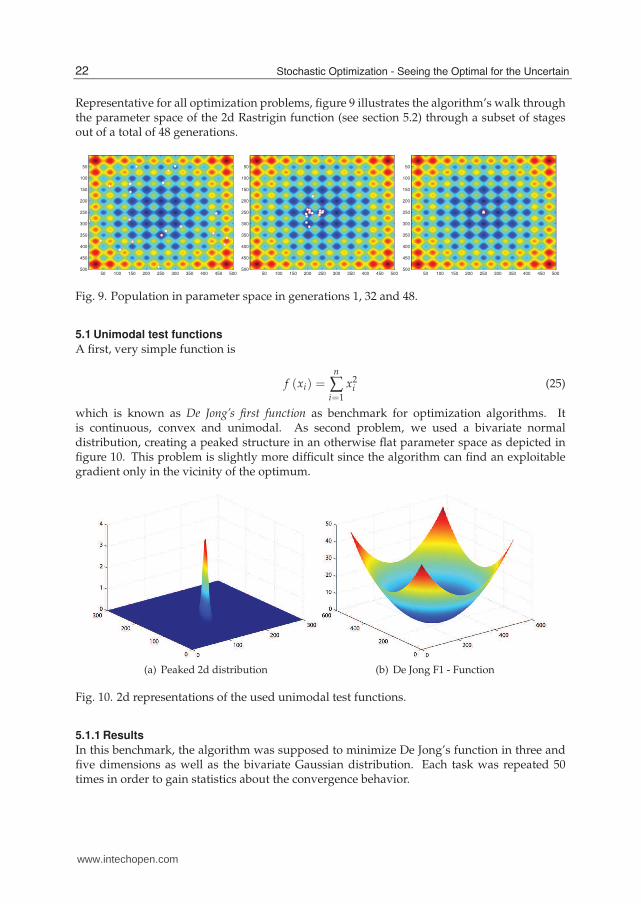
Representative for all optimization problems, figure 9 illustrates the algorithm’s walk throughthe parameter space of the 2d Rastrigin function (see section 5.2) through a subset of stagesout of a total of 48 generations.

50 100 150 200 250 300 350 400 450 500

50

100

150

200

250

300

350

400

450

50050 100 150 200 250 300 350 400 450 500

50

100

150

200

250

300

350

400

450

50050 100 150 200 250 300 350 400 450 500

50

100

150

200

250

300

350

400

450

500

Fig. 9. Population in parameter space in generations 1, 32 and 48.

5.1 Unimodal test functions

A first, very simple function is

f (xi) =n

∑i=1

x2i (25)

which is known as De Jong’s first function as benchmark for optimization algorithms. Itis continuous, convex and unimodal. As second problem, we used a bivariate normaldistribution, creating a peaked structure in an otherwise flat parameter space as depicted infigure 10. This problem is slightly more difficult since the algorithm can find an exploitablegradient only in the vicinity of the optimum.

(a) Peaked 2d distribution (b) De Jong F1 - Function

Fig. 10. 2d representations of the used unimodal test functions.

5.1.1 Results

In this benchmark, the algorithm was supposed to minimize De Jong’s function in three andfive dimensions as well as the bivariate Gaussian distribution. Each task was repeated 50times in order to gain statistics about the convergence behavior.

22 Stochastic Optimization - Seeing the Optimal for the Uncertain

www.intechopen.com

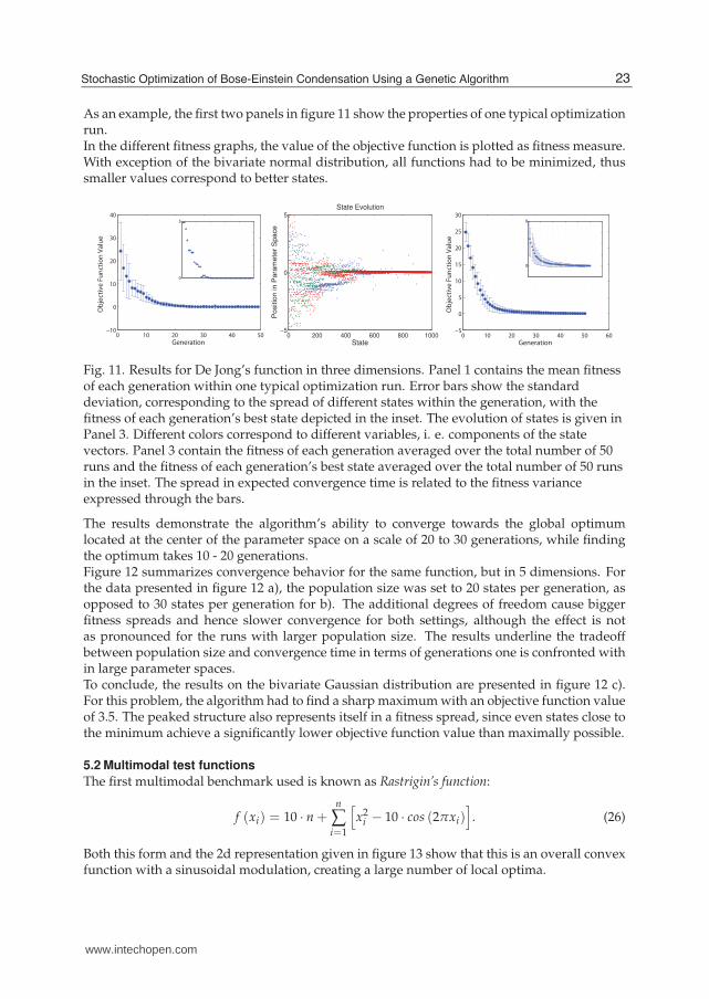
As an example, the first two panels in figure 11 show the properties of one typical optimizationrun.In the different fitness graphs, the value of the objective function is plotted as fitness measure.With exception of the bivariate normal distribution, all functions had to be minimized, thussmaller values correspond to better states.

0 10 20 30 40 50−10

0

10

20

30

40

Generation

Ob

ject

ive

Fu

nct

ion

Va

lue

0

5

0 200 400 600 800 1000−5

0

5

State

Positio

n in P

ara

mete

r S

pace

State Evolution

0 10 20 30 40 50 60−5

0

5

10

15

20

25

30

Generation

Ob

ject

ive

Fu

nct

ion

Va

lue

0

8

Fig. 11. Results for De Jong’s function in three dimensions. Panel 1 contains the mean fitnessof each generation within one typical optimization run. Error bars show the standarddeviation, corresponding to the spread of different states within the generation, with thefitness of each generation’s best state depicted in the inset. The evolution of states is given inPanel 3. Different colors correspond to different variables, i. e. components of the statevectors. Panel 3 contain the fitness of each generation averaged over the total number of 50runs and the fitness of each generation’s best state averaged over the total number of 50 runsin the inset. The spread in expected convergence time is related to the fitness varianceexpressed through the bars.

The results demonstrate the algorithm’s ability to converge towards the global optimumlocated at the center of the parameter space on a scale of 20 to 30 generations, while findingthe optimum takes 10 - 20 generations.Figure 12 summarizes convergence behavior for the same function, but in 5 dimensions. Forthe data presented in figure 12 a), the population size was set to 20 states per generation, asopposed to 30 states per generation for b). The additional degrees of freedom cause biggerfitness spreads and hence slower convergence for both settings, although the effect is notas pronounced for the runs with larger population size. The results underline the tradeoffbetween population size and convergence time in terms of generations one is confronted within large parameter spaces.To conclude, the results on the bivariate Gaussian distribution are presented in figure 12 c).For this problem, the algorithm had to find a sharp maximum with an objective function valueof 3.5. The peaked structure also represents itself in a fitness spread, since even states close tothe minimum achieve a significantly lower objective function value than maximally possible.

5.2 Multimodal test functions

The first multimodal benchmark used is known as Rastrigin’s function:

f (xi) = 10 · n +n

∑i=1

[

x2i − 10 · cos (2πxi)

]

. (26)

Both this form and the 2d representation given in figure 13 show that this is an overall convexfunction with a sinusoidal modulation, creating a large number of local optima.

23Stochastic Optimization of Bose-Einstein Condensation Using a Genetic Algorithm

www.intechopen.com

0 10 20 30 40 50 60−10

0

10

20

30

40

50

Generation

Ob

ject

ive

Fu

nct

ion

Va

lue

0

20

(a)

0 10 20 30 40 50 60−10

0

10

20

30

40

50

Generation

Ob

ject

ive

Fu

nct

ion

Va

lue

0

20

(b)

0 10 20 30 40 50 60−1

0

1

2

3

4

Generation

Ob

ject

ive

Fu

nct

ion

Va

lue

0

4

(c)

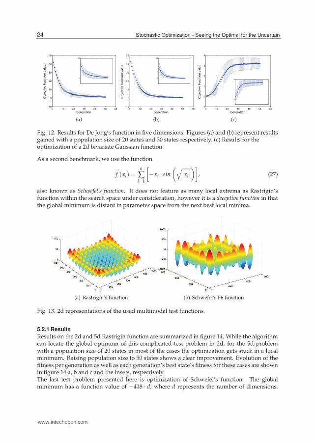
Fig. 12. Results for De Jong’s function in five dimensions. Figures (a) and (b) represent resultsgained with a population size of 20 states and 30 states respectively. (c) Results for theoptimization of a 2d bivariate Gaussian function.

As a second benchmark, we use the function

f (xi) =n

∑i=1

[

−xi · sin

(

√

|xi|)]

, (27)

also known as Schwefel’s function. It does not feature as many local extrema as Rastrigin’sfunction within the search space under consideration, however it is a deceptive function in thatthe global minimum is distant in parameter space from the next best local minima.

(a) Rastrigin’s function (b) Schwefel’s F6 function

Fig. 13. 2d representations of the used multimodal test functions.

5.2.1 Results

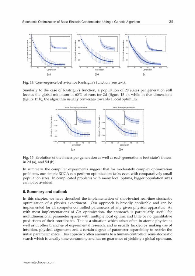
Results on the 2d and 5d Rastrigin function are summarized in figure 14. While the algorithmcan locate the global optimum of this complicated test problem in 2d, for the 5d problemwith a population size of 20 states in most of the cases the optimization gets stuck in a localminimum. Raising population size to 50 states shows a clear improvement. Evolution of thefitness per generation as well as each generation’s best state’s fitness for these cases are shownin figure 14 a, b and c and the insets, respectively.The last test problem presented here is optimization of Schwefel’s function. The globalminimum has a function value of −418 · d, where d represents the number of dimensions.

24 Stochastic Optimization - Seeing the Optimal for the Uncertain

www.intechopen.com

0 10 20 30 40 50 600

5

10

15

20

25

30

35

40

Generation

Ob

ject

ive

Fu

nct

ion

Va

lue

0

20

(a)

0 10 20 30 40 50 600

20

40

60

80

100

Generation

Ob

ject

ive

Fu

nct

ion

Va

lue

0

60

(b)

0 20 40 60 80 100 1200

20

40

60

80

100

Generation

Ob

ject

ive

Fu

nct

ion

Va

lue

0

60

(c)

Fig. 14. Convergence behavior for Rastrigin’s function (see text).

Similarly to the case of Rastrigin’s function, a population of 20 states per generation stilllocates the global minimum in 60 % of runs for 2d (figure 15 a), while in five dimensions(figure 15 b), the algorithm usually converges towards a local optimum.

0 10 20 30 40 50 60−1000

−800

−600

−400

−200

0

200

Mean �tness per generation

Generation

Ob

ject

ive

Fu

nct

ion

Va

lue

−900

−300

(a)

0 10 20 30 40 50 60−2000

−1500

−1000

−500

0

500

Mean �tness per generation

Generation

Ob

ject

ive

Fu

nct

ion

Va

lue

−1800

−400

(b)

Fig. 15. Evolution of the fitness per generation as well as each generation’s best state’s fitnessin 2d (a), and 5d (b).

In summary, the computer experiments suggest that for moderately complex optimizationproblems, our simple RCGA can perform optimization tasks even with comparatively smallpopulation sizes. In complicated problems with many local optima, bigger population sizescannot be avoided.

6. Summary and outlook

In this chapter, we have described the implementation of shot-to-shot real-time stochasticoptimization of a physics experiment. Our approach is broadly applicable and can beimplemented for all computer-controlled parameters of any given physical apparatus. Aswith most implementations of GA optimization, the approach is particularly useful formultidimensional parameter spaces with multiple local optima and little or no quantitativepredictions of their coordinates. This is a situation which arises often in atomic physics aswell as in other branches of experimental research, and is usually tackled by making use ofintuition, physical arguments and a certain degree of parameter separability to restrict theinitial parameter space. This approach often amounts to a human-controlled, semi-stochasticsearch which is usually time-consuming and has no guarantee of yielding a global optimum.

25Stochastic Optimization of Bose-Einstein Condensation Using a Genetic Algorithm

www.intechopen.com

Using the genetic-algorithm approach, we have seen rapid convergence to optimal parametersin 2- and 4-dimensional parameter spaces, and that the approach is robust even in the presenceof local optima and experimental noise. We envisage a number of possible augmentationsfor future implementations. Among these are the weighting of the fitness of a populationmember according to its experimental uncertainty, and the inclusion of qualitative physicalpredictions in some implementations. These predictions can then be progressively quantifiedwith each generation and used to steer mutations to speed up the search convergence. Infuture implementations, this method may also be extended to perform "optimal experimentalcontrol" that automatically finds the best experimental sequence to produce a defined targetquantum state. In conclusion, optimization using a genetic algorithm can be an efficient toolto improve the performance of a ‘real-life’ apparatus.

7. References

(n.d.). see atom traps world wide: http://www.uibk.ac.at/exphys/ultracold/atomtraps.htmland links therein.

Anderson, M. H., Ensher, J. R., Matthews, M. R., Wieman, C. E. & Cornell, E. A. (1995).Observation of Bose-Einstein condensation in a dilute atomic vapor, Science 269: 198.

Assion, A., Baumert, T., Bergt, M., Brixner, T., Kiefer, B., Seyfried, V., Strehle, M. & Gerber,G. (1998). Control of Chemical Reactions by Feedback-Optimized Phase-ShapedFemtosecond Laser Pulses, Science 282(5390): 919–922.URL: http://www.sciencemag.org/cgi/content/abstract/282/5390/919

Baker, J. E. (1985). Adaptive selection methods for genetic algorithms, Proceedings of the 1stInternational Conference on Genetic Algorithms, Lawrence Erlbaum Associates, Inc.,Mahwah, NJ, USA, pp. 101–111.

Baumert, T., Brixner, T., Seyfried, V., Strehle, M. & Gerber, G. (1997). Femtosecond pulseshaping by an evolutionary algorithm with feedback, Applied Physics B: Lasers andOptics 65: 779–782. 10.1007/s003400050346.URL: http://dx.doi.org/10.1007/s003400050346

Berman, P. R. (1996). Atom Interferometry, Academic Press, New York.Bose, S. N. (1924). Plancks gesetz und lichtquantenhypothese tex, Z. Phys. 26: 178.Bradley, C. C., Sackett, C. A., Tollett, J. J. & Hulet, R. G. (1995). Evidence of Bose-Einstein

condensation in an atomic gas with attractive interactions, Phys. Rev. Lett. 75: 1687.Bücker, R., Perrin, A., Manz, S., Betz, T., Koller, C., Plisson, T. , Rottmann, J., Schumm, T. &

Schmiedmayer, J. (2009). Single-particle-sensitive imaging of freely propagating ultracoldatoms, New J. Phys. 11, 103039 (2009).

Chu, S. (1998). The manipulation of neutral particles, Rev. Mod. Phys. 70: 685.Cohen-Tannoudji, C. N. (1998). Manipulating atoms with photons, Rev. Mod. Phys. 70: 707.Davis, K. B., Mewes, M.-O., Andrews, M. R., van Druten, N. J., Durfee, D. S., Kurn, D. M. &

Ketterle, W. (1995). Bose einstein condensation in a gas of sodium atoms, Phys. Rev.Lett. 75: 3969.

Davis, K. B., Mewes, M.-O., Ioffe, M. A., Andrews, M. R. & Ketterle, W. (1995). Evaporativecooling of sodium atoms, Phys. Rev. Lett. 74: 5202.

Davis, K., Mewes, M.-O. & Ketterle, W. (1995). An analytical model for evaporative cooling ofatoms, Appl. Phys. B 60: 155.

Einstein, A. (1925). Quantentheorie des einatomigen idealen gases. ii, Sitzungsber. Preuss. Akad.Wiss. Bericht 1: 3–14.

26 Stochastic Optimization - Seeing the Optimal for the Uncertain

www.intechopen.com

Folman, R., Krüger, P., Schmiedmayer, J., Denschlag, J. & Henkel, C. (2002). Microscopic atomoptics: from wires to an atom chip, Adv. At. Mol. Opt. Phys. 48: 263–356.

Fortagh, J. & Zimmermann, C. (2007). Magnetic microtraps for ultracold atoms, Rev. Mod.Phys. 79: 235.

Grimm, R., Weidemüller, M. & Ovchinnikov, Y. B. (2000). Optical dipole traps for neutralatoms, Adv. At. Mol. Opt. Phys. 42: 95.

Hänsel, W., Hommelhoff, P., Hänsch, T. W. & Reichel, J. (2001). Bose-Einstein condensation ona microelectronic chip, Nature 413: 498.

Haupt, R. (2000). Optimum population size and mutation rate for a simple real geneticalgorithm that optimizes array factors, Antennas and Propagation Society InternationalSymposium, 2000. IEEE 2: 1034–1037 vol.2.

Heine, D., Rohringer, W., Fischer, D., Wilzbach, M., Raub, T., Loziczky, S., Liu, X., Groth,S., Hessmo, B. & Schmiedmayer, J. (2010). A single-atom detector integrated onan atom chip: fabrication, characterization and application, New Journal of Physics12(9): 095005.URL: http://stacks.iop.org/1367-2630/12/i=9/a=095005

Herrera, F., Lozano, M. & Verdegay, J. L. (1998). Tackling real-coded geneticalgorithms operators and tools for behavioural analysis, Artificial Intelligence Review12(4): 265–319.URL: citeseer.ist.psu.eduherrera98tackling.html

Ketterle, W., Durfree, D. S. & Stamper-Kurn, D. M. (1998). Making, probing andunderstanding bose-einstein condensates, Contribution to the proceedings of the1998 Enrico Fermi summer school on Bose-Einstein condensation in Varenna, Italy,Academic Press, p. 1. and references therein.

Ketterle, W. & Zwierlein, M. W. (2008). Making, probing and understanding ultracold fermigases, Contribution to the proceedings of the 1998 Enrico Fermi summer school onultracold Fermi gases condensation in Varenna, Italy, IOS Press, p. 1. and referencestherein.

Luiten, O. J., Reynolds, M. W. & Walraven, J. T. M. (1996). Kinetic theory of the evaporativecooling of a trapped gas, Phys. Rev. A 53: 381.

Metcalf, H. J. (1999). Laser Cooling and Trapping, Springer Verlag, Heidelberg Berlin New York.Mühlenbein, H. & Schlierkamp-Voosen, D. (1993). Predictive models for the breeder genetic

algorithm, i.: continuous parameter optimization, Evol. Comput. 1(1): 25–49.Mühlenbein, H. & Schlierkamp-Voosen, D. (1995). Analysis of selection, mutation and

recombination in genetic algorithms, Evolution and Biocomputation, ComputationalModels of Evolution, Springer-Verlag, London, UK, pp. 142–168.

Ott, H., Fortagh, J., Schlotterbeck, G., Grossmann, A. & Zimmermann, C. (2001). Bose-Einsteincondensation in a surface microtrap, Phys. Rev. Lett. 87: 230401.

Phillips, W. D. (1998). Laser cooling and trapping of neutral atoms, Rev. Mod. Phys. 70: 721.Pohlheim, H. (1999). Evolutionre Algorithmen: Verfahren, Operatoren und Hinweise fr die

Praxis, Springer Verlag. ISBN 3-540-66413-0.Reichl, L. E. (1998). A Modern Course In Statistical Physics, John Wiley & Sons.Rohringer, W., Bücker, R., Manz, S., Betz, T., Koller, C., Göbel, M., Perrin, A., Schmiedmayer,

J. & Schumm, T. (2008). Stochastic optimization of a cold atom experiment using agenetic algorithm, Applied Physics Letters 93(26): 264101.URL: http://link.aip.org/link/?APL/93/264101/1

Rottmann, J. (2006). Towards a Single Atom Camera, Diploma thesis, University of Heidelberg.

27Stochastic Optimization of Bose-Einstein Condensation Using a Genetic Algorithm

www.intechopen.com

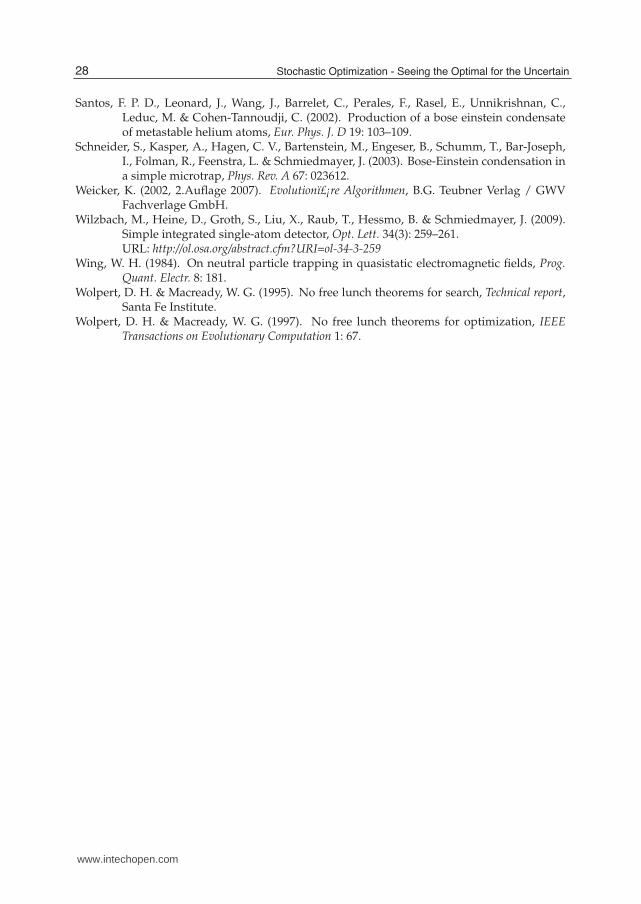
Santos, F. P. D., Leonard, J., Wang, J., Barrelet, C., Perales, F., Rasel, E., Unnikrishnan, C.,Leduc, M. & Cohen-Tannoudji, C. (2002). Production of a bose einstein condensateof metastable helium atoms, Eur. Phys. J. D 19: 103–109.

Schneider, S., Kasper, A., Hagen, C. V., Bartenstein, M., Engeser, B., Schumm, T., Bar-Joseph,I., Folman, R., Feenstra, L. & Schmiedmayer, J. (2003). Bose-Einstein condensation ina simple microtrap, Phys. Rev. A 67: 023612.

Weicker, K. (2002, 2.Auflage 2007). Evolutionre Algorithmen, B.G. Teubner Verlag / GWVFachverlage GmbH.

Wilzbach, M., Heine, D., Groth, S., Liu, X., Raub, T., Hessmo, B. & Schmiedmayer, J. (2009).Simple integrated single-atom detector, Opt. Lett. 34(3): 259–261.URL: http://ol.osa.org/abstract.cfm?URI=ol-34-3-259

Wing, W. H. (1984). On neutral particle trapping in quasistatic electromagnetic fields, Prog.Quant. Electr. 8: 181.

Wolpert, D. H. & Macready, W. G. (1995). No free lunch theorems for search, Technical report,Santa Fe Institute.

Wolpert, D. H. & Macready, W. G. (1997). No free lunch theorems for optimization, IEEETransactions on Evolutionary Computation 1: 67.

28 Stochastic Optimization - Seeing the Optimal for the Uncertain

www.intechopen.com

Stochastic Optimization - Seeing the Optimal for the UncertainEdited by Dr. Ioannis Dritsas

ISBN 978-953-307-829-8Hard cover, 476 pagesPublisher InTechPublished online 28, February, 2011Published in print edition February, 2011

InTech EuropeUniversity Campus STeP Ri Slavka Krautzeka 83/A 51000 Rijeka, Croatia Phone: +385 (51) 770 447 Fax: +385 (51) 686 166www.intechopen.com

InTech ChinaUnit 405, Office Block, Hotel Equatorial Shanghai No.65, Yan An Road (West), Shanghai, 200040, China

Phone: +86-21-62489820 Fax: +86-21-62489821

Stochastic Optimization Algorithms have become essential tools in solving a wide range of difficult and criticaloptimization problems. Such methods are able to find the optimum solution of a problem with uncertainelements or to algorithmically incorporate uncertainty to solve a deterministic problem. They even succeed in“fighting uncertainty with uncertainty†. This book discusses theoretical aspects of many such algorithmsand covers their application in various scientific fields.

How to referenceIn order to correctly reference this scholarly work, feel free to copy and paste the following:

W. Rohringer, D. Fischer, M. Trupke, J. Schmiedmayer and T. Schumm (2011). Stochastic Optimization ofBose-Einstein Condensation Using a Genetic Algorithm, Stochastic Optimization - Seeing the Optimal for theUncertain, Dr. Ioannis Dritsas (Ed.), ISBN: 978-953-307-829-8, InTech, Available from:http://www.intechopen.com/books/stochastic-optimization-seeing-the-optimal-for-the-uncertain/stochastic-optimization-of-bose-einstein-condensation-using-a-genetic-algorithm

© 2011 The Author(s). Licensee IntechOpen. This chapter is distributedunder the terms of the Creative Commons Attribution-NonCommercial-ShareAlike-3.0 License, which permits use, distribution and reproduction fornon-commercial purposes, provided the original is properly cited andderivative works building on this content are distributed under the samelicense.