Stochastic nonlinear shoaling of directional spectraalex/papers/JFM.pdf · In the case of a weakly...

J. Fluid Mech. (1997), vol. 345, pp. 79–99. Printed in the United Kingdom

c© 1997 Cambridge University Press

79

Stochastic nonlinear shoaling of directionalspectra

By Y. A G N O N1† AND A. S H E R E M E T2

1Department of Civil Engineering, Technion, Haifa 32000, Israel2CAMERI – Coastal and Marine Engineering Research Institute, Technion City,

Haifa 32000, Israel

(Received 17 May 1996 and in revised form 19 March 1997)

We derive a deterministic directional shoaling model and a stochastic directionalshoaling model for a gravity surface wave field, valid for a beach with parallel depthcontours accounting for refraction and nonlinear quadratic (three wave) interactions.A new phenomenon of non-resonant spectral evolution arises due to the medium in-homogeneity. The kernels of the kinetic equation depend on the bathymetry throughan integral operator. Preliminary tests carried out on laboratory data for a unidirec-tional case indicate that the stochastic model also works rather well beyond the regionwhere the waves may be regarded as nearly Gaussian. The limit of its applicabilityis decided by the dispersivity of the medium (relative to the nonlinearity). Goodagreement with both laboratory data and the underlying deterministic model is foundup to a value of about 1.5 for the spectral peak Ursell number. Beyond that only thedeterministic model matches the measurements.

1. IntroductionMuch of the work devoted in recent years to the study of shoaling wave fields

has been directed at the more tractable simplifications of the problem assumingunidirectionality, a mild bottom slope and weak dispersion. For the shallow-watercase one may cite the extensively tested Boussinesq-type model developed by Freilich& Guza (1984), having quadratic near-resonant interactions as the dominant energyexchange mechanism. The angular spectrum model derived by Suh, Dalrymple &Kirby (1990) falls in the class of Schrodinger-type models, valid at the deeper endof the beach, for a narrow spectrum and a dominant cubic-interaction nonlinearenergy exchange mechanism. The implied assumption of weak dispersion in theabove models is dropped in the work of Agnon et al. (1993). The evolution equationderived describes the shoaling of unidirectional arbitrary wide spectra all the wayfrom deep into shallow water, with no restriction on the dispersion of the waves.They assumed that refraction and the dominant nonlinear triad interactions are ofthe same order and neglected cubic and higher-order processes.

The degree of complexity of a model may be increased further by widening itsscope to include directional spread, breaking, mean flows – a plethora of processesmay be brought in. A deterministic model such as the ones mentioned has, however,limited utility. The sea state is essentially a stochastic process, and so in order to

† Present address: Centre for Computational Hydrodynamics (ICCH), Danish Hydraulic Insti-tute, Agern Alle 5, DK-2970 Hørsholm, Denmark.

80 Y. Agnon and A. Sheremet

obtain a viable wave forecast one has to run the model over and over again, on manydifferent initial data sets and average the results. Apart from the question of howmany such data sets one needs, deep-water wave forecasts and measured data comeusually in the form of power spectra estimates with no information about modalphases. Additional arbitrary assumptions about the missing data are then made –usually uniformly distributed random phases. The alternative, which we pursue here,is a stochastic shoaling model.

Regarding the system as stochastic, one seeks to describe its evolution by derivinga hierarchy of equations for the statistical moments, or equivalently the Fourier spacecumulants. This approach leads to the well-known closure problem fundamental tononlinear processes: the evolution equation for a moment of a given order dependson the moments of higher orders, and without additional assumptions one is left withan infinite set of equations to solve. This is the classical problem of closure.

In the case of a weakly nonlinear system such as water waves, one way to derivesome information from these equations is to use assumptions that discard all thecumulants of order higher than a specified value: the Gaussian approximation, forexample, amounts to neglecting cumulants higher than the second. Now, even if thewaves are Gaussian at one location, the evolution equation for the third-order momentcontains a fourth-order moment and a product of second-order moments (see Benney& Newell 1969), and so the third-order one should not be expected to remain zero.The shoaling processes in particular are characterized by a very fast evolution, in therange of at most a few tens of wavelengths, as the system evolves from dominantcubic to dominant quadratic near-resonant nonlinear interactions (a more intensiveenergy exchange mechanism) and from a dispersive to a weakly dispersive medium. Asa result the shallow-water waves exhibit very strongly phase-coupled Fourier modesand may by no means be regarded as Gaussian.

The first in a sequence of asymptotic closures for weakly nonlinear systems wasobtained by Benney & Saffman (1966), who were able to show that earlier results basedupon cumulant discarding assumptions were valid without the necessity of makingany restrictive assumptions. In a subsequent series of papers, Benney & Newell (1969)and Newell & Aucoin (1971) among others extended the original derivations tohigher-order closures and discussed further several specific systems. They describe themechanism that enables the closure as the action of two separate processes. The firstoccurs on a time (length) scale given by a characteristic period (wavelength) of thewaves involving the decoupling of the initial correlations due to the dispersive natureof the waves, and an approach to the Gaussian state as one might expect from theCentral Limit Theorem. The second process, occurring over longer scales, given bythe characteristic nonlinear time (length) scale, is one of regeneration of these highercumulants by nonlinear coupling. The dispersive nature of the medium is essential.Newell & Aucoin (1971) coined the phrase ‘semi-dispersive’ to denote non-dispersivemedia with more than one dimension; closure may still be obtained here with somequite fine tuning of the theory, due to the dispersive effect of waves travelling indifferent directions (these ideas appear in the stochastic directional shallow watermodel developed by Abreu, Larazza & Thornton 1992). In one-dimensional non-dispersive media there is no substitute for dispersion that can induce the decay ofthe initial correlations, which are conserved and enhanced by the nonlinearity, andno such closure seems possible.

In §2 we discuss the general restrictions imposed on the present model and makesome preparatory manipulations of the original governing equations. In the absenceof edge waves, the evolution equation derived by Agnon et al. (1993) is readily

Stochastic nonlinear shoaling 81

generalized to a nonlinear second-order shoaling one valid for obliquely incidentand directionally spread spectra, over a mildly sloped bottom. The extension to thedirectional deterministic shoaling model is straightforward and we give only its finalform. Starting from this equation, the present study derives, under the restrictionof parallel depth contours, a stochastic directional shoaling model that accounts fornearly resonant quadratic interactions, presented in §3.

The shoaling problem is one of an inhomogeneous medium. As the waves shoal,the locked, or bound, waves increase in magnitude, while the dispersion decreases.The kinetic equation for the energy spectrum has to account for the phase correlationstructure, which is reflected in the bispectrum, or in the distribution of the wavemotion at any frequency among the free waves and the locked waves at differentwavenumbers. We need an equation that has a ‘memory’, and indeed we obtain suchan equation. The kernels of the equation depend on the variation of the wavenumberswhich depend on the variation of the bottom depth. It is well known that in deepwater, or in water of constant depth, spectral evolution requires exact resonantconditions (which cannot be satisfied by triads of gravity waves). In contrast, thekernels obtained for shoaling waves have the form of ‘smeared delta functions’ andaccount for the important process of non-resonant triad interactions.

Section 4 presents experimental testing of the present model and comments on itsutility compared with the original deterministic one. The stochastic model appears tobe superior in several respects to the deterministic one, but further testing is needed.Conclusions are given in §5.

2. Formulation of the problemWe write the equations governing the irrotational flow of an inviscid fluid with a

free surface, after expanding the surface boundary conditions in power series aboutz = 0 and discarding all terms higher than quadratic in the wave steepness ε, whereε� 1. They are the Laplace equation:

∇2φ+ φzz = 0, − h 6 z 6 0, (2.1)

the bottom boundary condition:

φz + ∇h · ∇φ = 0, z = −h, (2.2)

the free-surface kinematic boundary condition:

ηt − φz + ∇ · (η∇φ) = 0, z = 0, (2.3)

and the free-surface dynamic boundary condition:

φt + gη + ηφtz + 12|∇φ|2 + 1

2(φz)

2 = 0, z = 0, (2.4)

where ∇ is the horizontal gradient and φ, η and h are the velocity potential, thefree-surface displacement and the local water depth, respectively. The origin of thereference frame is taken in deep water at the still water level, with the z-axis upwards.By eliminating η from (2.3)–(2.4) a new form of the system of governing equationsmay be obtained:

∇2φ+ φzz = 0, − h 6 z 6 0, (2.5)

φz + ∇h · ∇φ = 0, z = −h, (2.6)

φtt + gφz =

[− 1

2|∇φ|2 − 1

2(φz)

2 +1

gφtφzt

]t

− ∇ · (φt∇φ), z = 0, (2.7)


gη = −φt +1

gφtφzt − 1

2|∇φ|2 − 1

2(φz)

2, z = 0, (2.8)

where the first three equations form a closed system for φ, and η is given as a functionof φ via (2.8).

In what follows we make no assumptions regarding the shallowness of the water,which is to say kh may be O(1), with k the characteristic wavenumber, so that thelinear dispersion relation has to be used in its full form; we do assume that the beachslope is mild, that is |∇h| = O(ε) or smaller.

Next, we shall use a multiple scale approach, by defining the slow time t1 = εtwith the time derivative written accordingly as ∂t → ∂t + ε∂t1 , expand (2.5)–(2.8) andretain, for consistency, only terms up to O(ε2) with respect to the leading terms.

The velocity potential and the free-surface displacement will be expressed as

φ = φ0(x, y, t1) + εφ1(x, y, z, t, t1), (2.9)

η = εη0(x, y, t1) + εη1(x, y, t, t1). (2.10)

Here φ1 and η1 refer to the wave movement, and φ0, η0 denote the slowly varyingmean flow and set-down induced by the waves. It is assumed that ∇φ0 and ∇η0 areO(ε). The drift velocity potential is formally allowed to be of first order to account forthe growth of the current from O(ε2) in deep water to the same order as the orbitalvelocity in shallow water.

In order to separate two systems of equations, one for the slowly varying φ0 andη0, the ‘zero frequency’ mode, and another for the fast components φ1, η1, it will beuseful to eliminate the variable t by using the Fourier transform to go over to thefrequency domain:

φ(ω, t1) =

∫ ∞−∞φ(t, t1)e

−iωtdt, (2.11)

φ(t, t1) =1

2π

∫ ∞−∞φ(ω, t1)e

iωtdω. (2.12)

After some algebra, which is similar to the derivation in Agnon et al. (1993), thegoverning equations (2.1)–(2.4) yield for the fast components the system

∇2φ1 + φ1zz = 0, − h 6 z 6 0, (2.13)

φ1z + ∇h · ∇φ1 = 0, z = −h, (2.14)

−ω2φ1 + gφ1z = −2iωφ1t1 − {2iω∇φ0 · ∇φ1 + η0[ω2φ1z − g∇2φ1]}

+iω

4π

∫ ∞−∞

[∇φ(1)

1 · ∇φ(2)1 + φ

(1)1z φ

(2)1z + 2

ω1ω2

gφ

(1)1 φ

(2)1z

+2ω1

ω∇ · (φ(1)

1 ∇φ(2)1 )]δ(ω − ω1 − ω2)dω1dω2 + O(ε3), z = 0, (2.15)

−gη1 = iωφ1 + [φ1t1+ iωη0φ1z + ∇φ0 · ∇φ1]

+1

4π

∫ ∞−∞

[∇φ(1)

1 · ∇φ(2)1 + φ

(1)1zφ

(2)1z

+ 2ω1ω2

gφ

(1)1 φ

(2)1z

]×δ(ω − ω1 − ω2)dω1dω2 + O(ε3), z = 0, (2.16)

where the notation

φ(1)1 φ

(2)1 = φ1(x, y, z, ω1, t1)φ1(x, y, z, ω2, t1) (2.17)


was used in the integrands of (2.15)–(2.16). For the slowly varying components weshall prefer to use the surface boundary conditions in the form (2.3)–(2.4) and obtain[

η0t1+ ∇ · (h∇φ0)

]δ(ω) = − [∇ · (η0∇φ0)] δ(ω)

+1

4π2

∫ ∞−∞

iω

g∇ · (φ1∇φ∗1)dω + O(ε4), z = 0, (2.18)

[φ0t1

+ gη0

]δ(ω) = −

[12(∇φ0)

2]δ(ω)

− 1

8π2

∫ ∞−∞

[|∇φ1|2 + |φ1z |2 − 2

ω2

gφ1(φ1z )

∗]

dω + O(ε3), z = 0. (2.19)

The systems of equations (2.18)–(2.19) and (2.13)–(2.16) form the starting point forthe derivation of the evolution equation for a directional gravity wave spectrum thatwill be presented in the following sections.

3. The stochastic evolution equationThe main task in the derivation of the evolution equation for a shoaling directional

gravity wave spectrum is to reduce the three-dimensional system (2.13)–(2.16) to a

single equation by eliminating the vertical structure of the function φ1. Assumingthat no significant edge-wave modes are generated, a directional shoaling modelmay be obtained as a straightforward generalization of the method used by Agnonet al. (1993) for the unidirectional case. We shall not present the derivation here (thedetails may be found in Sheremet 1996), but cite only several definitions that areused as a starting point in the derivation and are also needed in what follows. Welook for a solution as a sum of a free and a locked wave forced by pairs of freewaves (higher-order locked waves are not effective on the characteristic scales of theshoaling process). The velocity potential is written as:

φ1 = φ1F + φ1L = ϕFZF +ε

µ

∫ ∞−∞ϕLZLδ(ω − ω1 − ω2)dω1dω2, (3.1a)

φ1|z=0 = ϕ = ϕF +ε

µ

∫ ∞−∞ϕLδ(ω − ω1 − ω2)dω1dω2, (3.1b)

where the functions ZF,L = cosh kF,L(z+ h)/ cosh(kF,Lh) are the free and locked wavesvertical structure respectively, with kL = kF (ω1)± kF (ω2) and kF,L = |kF,L|.

The measure of the departure of the locked wave from the free wave character isgiven by the detuning parameter:

µ =|kF (ω)− (kF (ω1)± kF (ω2))|

|kF (ω)| , (3.2)

which evolves from O(1) in deep water, where the locked wave is of second order withrespect to the free wave, to O(ε) in shallow water as the system approaches quadraticresonance and the locked wave grows to the same order as the free wave. We havetherefore taken it explicitly in (3.1) of order ε/µ. The absence of edge waves allowsone to use a formal WKB expansion that leads (see the references cited above) to theevolution equation for the complex amplitude of ϕ:


∂A

∂t1+ 1

2∇ · CgA+ C g · ∇A+ i

[ g2ω

(k2 − σ4)η0 + k · ∇φ0

]A

=

∫ ∞−∞W (0,1,2)A1A2 exp

[i

∫(k − k1 − k2)dx

]δω0:1,2dω1dω2, (3.3a)

W (0,1,2) =1

8π

(2k1 · k2 + (σ1σ2)

2 + k21

σ2

σ+ k2

2

σ1

σ− σ2σ1σ2

), (3.3b)

σ2j =

ω2j

g= kj tanh(kjh) (3.3c)

where

ϕ = Ae−i∫kdx,

δω0:1,2 is shorthand for δ(ω − ω1 − ω2) and Cg = Cgk/k is the vector group velocity.For the unidirectional case of waves propagating normally to the shore, this coincideswith the result obtained by Agnon et al. (1993). When the depth variation in thedirection parallel to the beach is much slower than the slope normal to the beach, thewavenumber in the long-shore direction is another constant of motion, in additionto the frequency. Going over to the long-shore wavenumber domain turns out tosimplify considerably the description of directional spectra (the idea is described indetail in Suh et al. 1990). Denote the cross- and long-shore coordinates by x andy respectively, and the corresponding wavenumbers kx and κ. Formally, taking theFourier transform of the evolution equation over y amounts to bringing κ and ωonto an equal footing in (3.3), which gives

∂A

∂t1+

1

2

∂

∂x

(kx

kCg

)A+ Cg

kx

k

∂A

∂x+ i[ g

2ω(k2 − σ4)η0 + kxφ0x

]A

=

∫ ∞−∞W (0,1,2)A1A2 exp

[−i

∫ x

−∞(k − k1 − k2)dx

]δω0:1,2δ

κ0:1,2dω1dω2dκ1dκ2 (3.4a)

W (0,1,2) =1

8π

[2k1 · k2 + (σ1σ2)

2 + k21

σ2

σ+ k2

2

σ1

σ− σ2σ1σ2

]. (3.4b)

The wavenumber squared is k2i = k2

x,i + κ2i . It should be noted that the function

A = A(x, x1, y, y1, ...ω, t1, ...) appearing in equation (3.3) is different from the one in(3.4), where A = A(x, x1, ..., κ, ω, t1, ...). Since, however, both functions play the samerole – an amplitude – in the derivation of the evolution equation, to keep the formulaesimple we preferred to use the same notation for both.

Equation (3.4), valid for a mildly sloping beach all the way from deep into shallowwater, is the starting point for the derivation of the stochastic model. It should bestressed that use is made of it in the following derivation only in the domain wherethe medium is still dispersive, that is beyond the region where Airy’s theory for verylong waves in shallow water is applicable (this is the ‘semi-dispersive’ domain of themodel developed by Abreu et al. 1992 and requires special treatment). We shall firstbring it to a discrete form, needed also for numerical integration purposes, by writingfor the velocity potential the Fourier expansion

φ = − i

2

∞∑l=−∞

∞∑f=1

[Afl exp

[i

(∫kx,fldx+ κly − ωft

)]−A∗fl exp

[−i

(∫kx,fldx+ κly − ωft

)]], (3.5)


which yields for the function ϕ the expression

ϕ = − i

2(2π)2

∞∑l=−∞

∞∑f=1

[Afl exp

(i

∫kx,fldx

)δ(ω + ωf)δ(κ− κl)

−A∗fl exp

(−i

∫kx,fldx

)δ(ω − ωf)δ(κ+ κl)

],

with the mesh in the (ω, κ) domain defined as ωf = fω1 and κl = lκ1, f = 1, 2, . . .(positive integer) and l = . . . ,−2, 1, 0, 1, 2, . . . (integer), and δ the Kronecker symbol.Substitution of the above into (3.4) gives the discrete equation

∂Afl

∂t1+

1

2

∂

∂x

(Cgx,fl

)Afl + Cgx,fl

∂Afl

∂x+ i

[g

2ω(k2f − σ4

f)η0 + kx,fl∂φ0

∂x

]Afl

= −i∑f1 ,l1

∑f2 ,l2

W (0,1,2)Af1l1Af2l2 exp

[−i

∫ x

−∞∆0:1,2dx

]δω0:1,2δ

κ0:1,2

−i∑f1 ,l1

∑f2 ,l2

2W (0,−1,2)Af1l1Af2l2 exp

[i

∫ x

−∞∆2:0,1dx

]δω2:0,1δ

κ2:0,1, (3.6a)

W (0,±1,2) =1

8

[±2kf1l1 · kf2l2 + (σf1

σf2)2 + k2

f1

σf2

σf± k2

f2

σf1

σf∓ σ2

fσf1σf2

], (3.6b)

where Cgx,fl = Cg,fkx,fl/kf is the cross-shore component of the group velocity and

∆0:1,2 = kx,fl − kx,f1l1 − kx,f2l2 . By introducing the variable Bfl = C1/2gx,flAfl one obtains,

for the steady-state case, the somewhat simpler form

dBfldx

+i

Cgx,fl

[g

2ωf(k2f − σ4

f)η0 + kfφ0x1

]Bfl

= −i∑f1 ,l1

∑f2 ,l2

W (0,1,2)Bf1l1Bf2l2 exp

[−i

∫ x

−∞∆0:1,2dx

]δω0:1,2δ

κ0:1,2

−i∑f1 ,l1

∑f2 ,l2

2W (0,−1,2)B∗f1l1Bf2l2 exp

[i

∫ x

−∞∆2:0,1dx

]δω2:0,1δ

κ2:0,1, (3.7a)

W (0,±1,2) = W (0,±1,2)

(Cgx,flCgx,f1l1Cgx,f2l2

)−1/2. (3.7b)

A special modification of a rather standard procedure will be used in what followsto derive the stochastic model (see Sheremet 1996 for the details). Multiply equation(3.7) by B∗fl and add to the complex conjugate of the same equation to obtain

d|Bfl |2dx

= 2∑f1 ,l1

∑f2 ,l2

W (0,1,2)Im

[B∗flBf1l1Bf2l2 exp

(−i

∫ x

−∞∆0:1,2dx

)]δω0:1,2δ

κ0:1,2

−2∑k,f

2W (0,−1,2)Im

[B∗flB

∗f1l1Bf2l2 exp

(i

∫ x

−∞∆2:0,1dx

)]δω2:0,1δ

κ2:0,1 (3.8)

where Im[F] denotes the imaginary part of F .Under the common assumption that the modal phases are to leading order un-

correlated, the right-hand side of (3.8) cancels in the average yielding the linearapproximation to the energy flux conservation equation. In order to obtain a descrip-tion of the effect of the nonlinear interactions one has to go to higher-order terms, and


evaluate the derivative of products of the type ∂ (B∗BB) /∂x using equation (3.7) andaverage again. Benney & Saffman (1966) have shown that for dispersive waves theleading-order contribution to the kinetic equation comes from products with repeatedindices. Using the notation 〈. . .〉 for the ensemble average one can write the relations

d

dx〈B∗flBf1l1Bf2l2〉 = 2i

[W (0,1,2)〈|Bf1l1 |2〉〈|Bf2l2 |2〉+ W (1,−2,0)〈|Bf2l2 |2〉〈|Bfl |2〉

+W (2,−1,0)〈|Bf1l1 |2〉〈|Bfl |2〉]

exp

[i

∫ x

−∞∆0:1,2dx

]δω0:1,2δ

κ0:1,2, (3.9a)

d

dx〈B∗flB∗f1l1

Bf2l2〉 = −2i[W (0,−1,2)〈|Bf1l1 |2〉〈|Bf2l2 |2〉+ W (1,−0,2)〈|Bf2l2 |2〉〈|Bfl |2〉

+W (2,1,0)〈|Bf1l1 |2〉〈|Bfl |2〉]

exp

[−i

∫ x

−∞∆2:0,1dx

]δω2:0,1δ

κ2:0,1, (3.9b)

which may be integrated with respect to x by assuming that the spectrum variesslowly with x. Integrating by parts, we may neglect the terms in which the derivativesof the spectrum appear, since they are O(ε2) smaller. For simplicity we neglect thebispectrum in deep water (which is very small in a nearly Gaussian sea). It can beshown that this does not affect the shoaling spectrum.

After integration and substitution back into equation (3.8) one obtains the equation:

d

dx〈|Bfl |2〉 = 4

∑f1 ,l1

∑f2 ,l2

[W (0,1,2)〈|Bf1l1 |2〉〈|Bf2l2 |2〉+ W (1,−2,0)〈|Bf2l2 |2〉〈|Bfl |2〉

+W (2,−1,0)〈|Bf1l1 |2〉〈|Bfl |2〉]W (0,1,2)Re[J0:1,2]δω0:1,2δ

κ0:1,2

+8∑f1 ,l1

∑f2 ,l2

[W (0,−1,2)〈|Bf1l1 |2〉〈|Bf2l2 |2〉+ W (1,−0,2)〈|Bf2l2 |2〉〈|Bfl |2〉

+W (2,1,0)〈|Bf1l1 |2〉〈|Bfl |2〉]W (0,−1,2)Re[J2:0,1

]δω2:0,1δ

κ2:0,1. (3.10)

Here Re[F] means the real part of F . The function J appearing in (3.10) is definedas:

J0:1,2 = exp

[−i

∫ x

−∞∆0:1,2dx

′] ∫ x

−∞exp

[i

∫ x′

−∞∆0:1,2dζ

]dx′. (3.11)

With a change of variables, we get

J0:1,2 =

∫ ∞−∞H(t) exp

[i

∫ t

0

∆0:1,2dζ

]dt, (3.12)

where H is the Heaviside function. J satisfies the simple differential equation

d

dxJ0:1,2 + i∆0:1,2J0:1,2 = 1. (3.13)

In (3.12) the dependence of J on x is by way of the argument of ∆0:1,2 = ∆0:1,2(x− ζ).If the wavenumbers do not depend on the x-coordinate, as for the case of deep water,it may be seen from (3.12) that J is simply

J0:1,2 = πδ(∆0:1,2)−i

∆0:1,2

. (3.14)

In the case of constant depth Re[J0:1,2

]= 0 and there is no triad interaction. For

waves in which triad interaction is possible, the kernel for the interaction (which plays


a role similar to that of Re[J0:1,2

]), like the kernel for traditional four-wave interac-

tion, is of a homogeneous medium, and the information of the global bathymetry doesnot enter the picture. In the case of an inhomogeneous medium, there is considerablebuild-up of the bispectrum (through the generation of large locked waves). The infor-mation about the bispectrum is implicitly brought in through the function J, whichstores the history of the bathymetry. Equation (3.10) can easily be generalized toinclude the term due to the initial bispectrum, when the sea is not initially Gaussian.We then see that this term gives rise to recurrence in the spectra of waves over a flatbottom.

The equation may also be written in terms of energy fluxes. Denote by Ffl theaveraged linear energy flux corresponding to the Fourier mode (f, l), which is relatedto the former variable 〈|B|2〉 by

Ffl =1

2

ω2f

g2〈|Bfl |2〉 (3.15)

and the new form of the equation (3.10) is

d

dxFfl = 8

∑f1 ,l1

∑f2 ,l2

[T (0,1,2)Ff1l1Ff2l2 + T (1,−2,0)Ff2l2Ffl + T (2,−1,0)Ff1l1Ffl

]T (0,1,2)

×Re[J0:1,2

]δω0:1,2δ

κ0:1,2

+16∑f1 ,l1

∑f2 ,l2

[T (0,−1,2)Ff1l1Ff2l2 + T (1,−0,2)Ff2l2Ffl + T (2,1,0)Ff1l1Ffl

]T (0,−1,2)

×Re[J2:0,1

]δω2:0,1δ

κ2:0,1, (3.16)

with the new kernel function T defined as

T (0,±1,2) =gωf

ωf1ωf2

W (0,±1,2). (3.17)

Equation (3.16) is the main result of the present work. To integrate it numericallyone needs only the power spectrum of the deep-water wave field and the beachbathymetry.

Both for reasons of simplicity and because of scarcity of data, preliminary testing ofthe stochastic directional shoaling model (3.16) has been conducted on the simplifiedunidirectional version that is obtained under the assumption that the waves propagatenormally to the shore. For this particular case (3.16) reads

d

dxFf = 8

∑f1 ,f2

[T 0,1,2Ff1

Ff2+ T (1,−2,0)Ff2

Ff + T (2,−1,0)Ff1Ff]T (0,1,2)

×Re[J0:1,2

]δω0:1,2

+16∑f1 ,f2

[T (0,−1,2)Ff1

Ff2+ T (1,−0,2)Ff2

Ff + T (2,1,0)Ff1Ff]T (0,−1,2)

×Re[J2:0,1

]δω2:0,1. (3.18)

Equations (3.18) and (3.13) form a closed system that may be integrated numericallygiven initial conditions in the form of a deep-sea power spectrum of the incomingwave field (since in this approximation the evolution of the wave field has no feedbackfrom the evolution of the mean variables η0 and φ0 we shall ignore them in whatfollows).

An illustration of the idea used in the integration of (3.9) is given in figure 1(a)


(a)

0.50

0

–0.50

–1.0

1.0

(b)

5

0

10

Bathymetry (slopes = 1%)

–10

–30

Position (m)

–20

0 500 1000 1500 2000 2500

Nor

mal

ized

fac

tors

Re(

*)

Dep

th(m

)

Figure 1. The evolution of the two factors in (3.9) plotted as functions of position for the peak andits second harmonic interaction (JONSWAP spectrum, (Tpeak = 12.2 s, Hsig = 2.2 m)), shoaling overa 1% sloped bottom. (a) The term in the square brackets (dashed line) and the imaginary part ofthe exponential term (solid line). (b) The function J computed for the same triad.

where the evolution of the term in square brackets is plotted as a function of x for atypical spectrum (peak period 12 s – see §4.2). The interaction is of the triad (f, f, 2f),f being the spectral peak frequency. The bottom slope is 1%. Also plotted is theimaginary part of the exponential term. It is seen that in this case the latter variesmuch faster than the former and we may ‘take’ the slowly varying term outside theintegration. This scale separation is less pronounced in less dispersive situations (thatis, larger Ursell parameter, see §4). Still, we find good agrreement with measurementsand with the deterministic model. The evolution of J for the same triad is plottedin figure 1(b). It is seen that the spatial resolution required is largely reduced by notresolving the bispectrum.

Numerical examples using the simplified version of (3.18) are discussed in the nextsection.

4. Comparison with laboratory measurementsWe have tested the performance of the numerical stochastic model against two

sets of laboratory simulations: one for a bimodal spectrum evolution data froman experiment carried out by WES Research Division (a detailed presentation ofthe measurements is available in Briggs, Smith & Green 1991); and one for a morerealistic unimodal shoaling spectrum (JONSWAP) from a set of measurements carried


out at CAMERI - Coastal and Marine Engineering Research Institute, Technion (fordetails see Sheremet & Stiassnie 1996).

Tests conducted on simulated data have shown that the number of modes chosen todescribe the spectral evolution is not a critical parameter as long as the main featuresof the initial spectrum are preserved. The number of equations in the system growsroughly like N2, where N is the number of Fourier modes, and although part of theequations (those for the J function) may be integrated separately, as they dependonly on the bathymetry and the modal frequencies, the numerical effort can still berather large. Therefore, the spectral analysis for the simulations was tuned to obtainsmoother and lower-resolution spectral estimates, and the tail part of the spectrumwas discarded (the energy in the discarded part was in both cases presented muchless than 1% of the total energy). The number of modes was thus reduced to 30 forthe bimodal simulations and 60 for the unimodal ones. In both cases, 50 independentruns were averaged to obtain the spectral evolution. Standard spectral analysis wasused in both cases: each individual sequence was windowed using a Hanning window,then transformed to the frequency domain using standard FFT routines. The samplespectral densities were then averaged to obtain the power spectra.

The results of the stochastic numerical model were also compared to that of theaveraged deterministic model derived by Agnon et al. (1993). We present the resultsof the runs only for one (the first) set of data, as reference – the deterministic modelbehaved consistently throughout. From measurements in time series form, the correctinitial phases are readily derived; we note, however, that in general the initial datafor such a model might well be expected to come from sources that give only spectraldensity information (an open-sea wave forecasting model for example).

To increase the readability of the numerical results, three frequency domains wereseparated by vertical lines: a ‘long waves’ a ‘medium waves’ and a ‘short waves’band. The limits of each band were defined differently from case to case. It shouldbe stressed that this division is done here in order to separate the spectral peaks. A‘band significant height’ may be defined by the relation

H2domain = 16

∫ f2

f1

S(f)df (4.1)

where domain stands for ‘long’, ‘medium’ or ‘short’ and f1 and f2 are the correspondingfrequency limits. The above parameter may be regarded as a convenient way todescribe the energy within a certain frequency interval.

As pointed out before, there is no sense in looking for a stochastic model for thecase of unidirectional non-dispersive media. The usefulness of (3.18) depends on howclose the actual data are to this case. One parameter that gives a measure of howclose the case is to Airy’s theory of very long waves in shallow water (non-dispersivemedium) is the Ursell number Ur = a/(k2h3) with a, k and h the characteristicamplitude and wavenumber of the wave field and the local depth respectively. Thecomputed Ursell numbers (based on the ‘band significant heights’ and peak frequency)are given in the plots next to each of the peaks.

As a simple test of the statistical properties of the measurements, we compare theprobability distribution of the normalized water level variable (zero mean and unitstandard deviation) to the normal probability distribution, together with the evolutionof the bicoherence. The natural evolution of the wave field during shoaling is quiteobvious in both cases: the waves peak and develop longer and shallower troughs, ineffect evolving towards a train of solitons. To obtain a measure of the modal phase


correlations we used the bispectral analysis techniques, e.g. Elgar & Guza (1985). Thebispectrum is defined as the Fourier transform of the third-order cumulant:

B(ω1, ω2) =

(1

2π

)2 ∫ ∞−∞S(τ1, τ2) exp [−iω1τ1 − iω2τ2] dτ1dτ2,

S(τ1, τ2) = 〈η(t)η(t+ τ1)η(t+ τ2)〉

(4.2)

with S the third-order cumulant and the angular brackets the averaging operator.For discretely sampled data the digital bispectrum is

B(ωk, ωj) = 〈AωkAωjA∗ωk+ωj 〉. (4.3)

The bicoherence (the magnitude of the bispectrum normalized to the [0, 1] interval),which is a more convenient way to represent the phase correlation information, isdefined by

b2(ωk, ωj) =|B(ωk, ωj)|2

〈|AωkAωj |2〉〈|Aωk+ωj |2〉. (4.4)

For a Gaussian field the bicoherence is zero. The bicoherence will exhibit a pronouncedpeak at the frequencies (ωk, ωj) if the modes k and j are phase correlated.

4.1. Bimodal spectral evolution

From the laboratory data gathered by the WES Research Division (Briggs et al.1991), the only case available to us that seemed to fit most of the restrictions imposedin the derivation of the model equation (3.18) – i.e. propagation normal to the shoreover nearly parallel depth contours, with no breaking – was code named D81, abimodal case with two peaks at the frequencies 0.4 and 0.8 Hz. The data consist oftime series, 6500 records each (sampling frequency of 10 Hz) measured in an arrayof 20 locations of which 10 locations were distributed normally to the shore.

Figure 2 shows the evolution of the leading-order energy flux density (an invariantfor a linear evolution). The plots indicate that the nonlinear evolution starts at about26 cm depth, the fourth location in the cross-shore array. Breaking or other dissipationmechanisms appear to become active around the depth of 19 cm. We shall thereforeomit the deeper locations in our presentation.

Figure 3 shows the probability distribution of the normalized water level againstthe normal distribution, together with the bicoherence at the same gauges. It seemsthat the Gaussian approximation is still valid only up to the depth of 29–25 cm.The evolution of the bicoherence given in figure 3 seems to confirm part of theexpectations. Again, the sudden degradation of the correlations seen at the 15 cmdepth indicates some dissipation.

The performance of the model (3.18) may be seen in figure 4 where the predictedpower spectral density is plotted against the measured one. The predictions followrather closely the measurements up to the depth of 15 cm. The results seem to indicatea value of Ur of about 1.5 as a possible threshold for the transition from a dispersiveto non-dispersive medium.

Figure 5 shows the behaviour of the model derived by Agnon et al. (1993). Theagreement with measurements is very good in the full range of depths, especially ifwe note that breaking begins at about 0.2 m depth. As noted above, in this regionthere is already dissipation of energy.


5

4

3

2

1

0

(×10–3)

0.5 1.0 1.5 2.0 2.5

(a) h = 0.4

Ene

rgy

flux

den

sity

5

4

3

2

1

0

(×10–3)

0.5 1.0 1.5 2.0 2.5

(c) h = 0.29

Ene

rgy

flux

den

sity

5

4

3

2

1

0

(×10–3)

0.5 1.0 1.5 2.0 2.5

(e) h = 0.23

Ene

rgy

flux

den

sity

Frequency (s–1)

5

4

3

2

1

0

(×10–3)

0.5 1.0 1.5 2.0 2.5

(b) h = 0.36

5

4

3

2

1

0

(×10–3)

0.5 1.0 1.5 2.0 2.5

(d) h = 0.26

5

4

3

2

1

0

(×10–3)

0.5 1.0 1.5 2.0 2.5

( f ) h = 0.19

Frequency (s–1)

Figure 2. WES data set. Energy flux density evolution (a–f); the energy flux density is aninvariant for linear shoaling.

4.2. Unimodal spectrum (JONSWAP) simulations

Being designed as simulations of typical storms in the Eastern Mediterranean, theCAMERI laboratory simulations (Sheremet & Stiassnie 1966) are, in a sense, a muchmore interesting testing ground for the present model. The experiment was carriedout in the CAMERI towing tank, using a bi-dimensional model (scale 1: 40) of thebathymetry in front of the Acre Harbour. The evolution of the waves was monitoredfrom 30 m depth to 6 m depth (prototype), at 13 locations uniformly distributed alonga region roughly divided into two segments: the first having a slope of about 5%, from30 to 8 m depth, and the second with a slope of about 1%, from 8 to 6 m depth. Mostof the nonlinear evolution occurred within the second shorter and shallower segment.A JONSWAP spectrum with γ = 2.8, characteristic of waves measured in the EasternMediterranean, was used to simulate the deep water spectral density. A total of 10storm simulations with different peak periods and significant heights (ranging from 9 sto 14 s and from 1.5 m to 3 m respectively – care was taken to prevent wave-breaking)were performed with the aim to provide data for testing the stochastic model. Thetwo cases we present (Tpeak = 12.2 s, Hsig = 2.2 m) and (Tpeak = 14.4 s, Hsig = 2.0 m)are representative of the overall performance of the model.

All the numbers that appear in what follows refer to the prototype scale.


0.6

0.4

0.2

0–4 –2 0 2 4

(a) h = 0.399 m

Pro

babi

lity

dis

trib

utio

n

2

1

0 1 2 3 4

(b) h = 0.399 m

Freq

uenc

y (s

–1)

0.6

0.4

0.2

0–4 –2 0 2 4

(c) h = 0.192 m

Pro

babi

lity

dis

trib

utio

n

2

1

0 1 2 3 4

(d) Depth: 0.192 mFr

eque

ncy

(s–1

)

0.6

0.4

0.2

0–4 –2 0 2 4

(e) h = 0.128 m

Pro

babi

lity

dis

trib

utio

n

2

1

0 1 2 3 4

( f ) Depth: 0.128 m

Freq

uenc

y (s

–1)

Frequency (s–1)Free surface (normal)

Figure 3. WES data set. Normalized time series histograms against the normal Gaussian distribution(a, c, e). The bicoherence at the same depths (b, d, f). The level curves are drawn at 0.2 increments.


2.0

1.5

1.0

0.5

0 1.5 2.0 2.5

Spe

ctra

l den

sity

(m

2 s) (×10–3)

Ur = 0.2

Ur = 1.1

2.0

1.5

1.0

0.5

0 1.5 2.0 2.5

(×10–3)Ur = 0.54

Ur = 2.7

meas.Hl = 0.043Hm = 0.08Hs = 0.036

modelHl = 0.043Hm = 0.08Hs = 0.036

(a) h = 0.3993 m

meas.Hl = 0.046Hm = 0.073Hs = 0.044

modelHl = 0.047Hm = 0.08Hs = 0.037

(b) h = 0.2591 m

2.0

1.5

1.0

0.5

0 1.5 2.0 2.5

Spe

ctra

l den

sity

(m

2 s) (×10–3)

Ur = 0.74

Ur = 3.5

2.0

1.5

1.0

0.5

0 1.5 2.0 2.5

(×10–3)Ur = 1.1

Ur = 4.8

meas.Hl = 0.046Hm = 0.069Hs = 0.046

modelHl = 0.049Hm = 0.08Hs = 0.038

(c) h = 0.2256 m

meas.Hl = 0.044Hm = 0.062Hs = 0.044

modelHl = 0.051Hm = 0.079Hs = 0.04

(d) h = 0.192 m

2.0

1.5

1.0

0.5

0 1.5 2.0 2.5

Spe

ctra

l den

sity

(m

2 s) (×10–3)

Ur = 1.7

Ur = 6.9

2.0

1.5

1.0

0.5

0 1.5 2.0 2.5

(×10–3)

Ur = 2.9

Ur = 9.9

meas.Hl = 0.043Hm = 0.057Hs = 0.045

modelHl = 0.055Hm = 0.076Hs = 0.045

(e) h = 0.1585 m

meas.Hl = 0.042Hm = 0.05Hs = 0.048

modelHl = 0.06Hm = 0.07Hs = 0.056

( f ) h = 0.128 m

Frequency (s–1) Frequency (s–1)

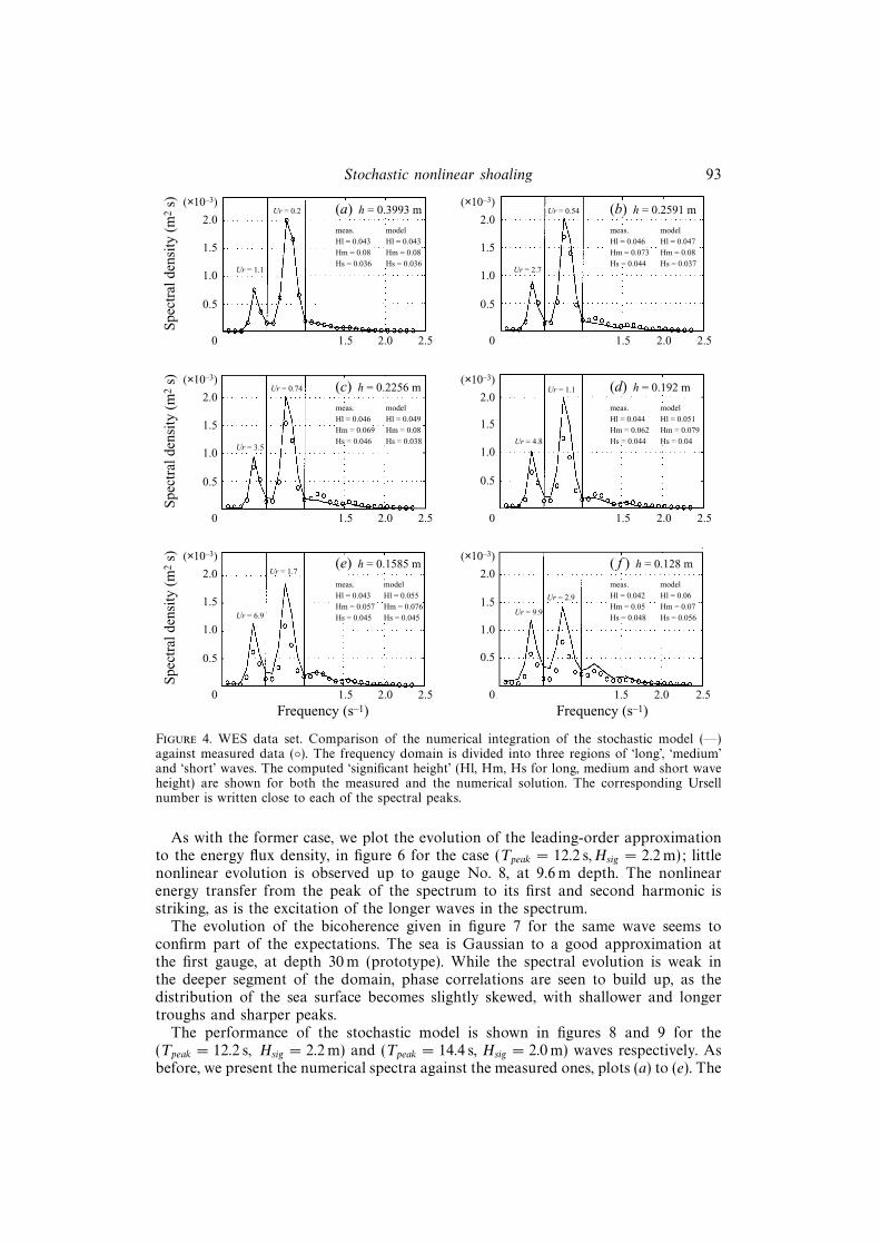
Figure 4. WES data set. Comparison of the numerical integration of the stochastic model (—)against measured data (◦). The frequency domain is divided into three regions of ‘long’, ‘medium’and ‘short’ waves. The computed ‘significant height’ (Hl, Hm, Hs for long, medium and short waveheight) are shown for both the measured and the numerical solution. The corresponding Ursellnumber is written close to each of the spectral peaks.

As with the former case, we plot the evolution of the leading-order approximationto the energy flux density, in figure 6 for the case (Tpeak = 12.2 s, Hsig = 2.2 m); littlenonlinear evolution is observed up to gauge No. 8, at 9.6 m depth. The nonlinearenergy transfer from the peak of the spectrum to its first and second harmonic isstriking, as is the excitation of the longer waves in the spectrum.

The evolution of the bicoherence given in figure 7 for the same wave seems toconfirm part of the expectations. The sea is Gaussian to a good approximation atthe first gauge, at depth 30 m (prototype). While the spectral evolution is weak inthe deeper segment of the domain, phase correlations are seen to build up, as thedistribution of the sea surface becomes slightly skewed, with shallower and longertroughs and sharper peaks.

The performance of the stochastic model is shown in figures 8 and 9 for the(Tpeak = 12.2 s, Hsig = 2.2 m) and (Tpeak = 14.4 s, Hsig = 2.0 m) waves respectively. Asbefore, we present the numerical spectra against the measured ones, plots (a) to (e). The


2.0

1.5

1.0

0.5

0 0.5 2.0 2.5

Spe

ctra

l den

sity

(m

2 s) (×10–3)

Ur = 0.2

Ur = 1.1

2.0

1.5

1.0

0.5

0 1.5 2.0 2.5

(×10–3) Ur = 0.56

Ur = 2.6

meas.Hl = 0.043Hm = 0.081Hs = 0.033

modelHl = 0.043Hm = 0.081Hs = 0.033

(a) h = 0.3993 m

meas.Hl = 0.046Hm = 0.074Hs = 0.041

modelHl = 0.049Hm = 0.077Hs = 0.041

(b) h = 0.2591 m

2.0

1.5

1.0

0.5

0 1.5 2.0 2.5

Spe

ctra

l den

sity

(m

2 s) (×10–3) Ur = 0.76

Ur = 3.3

2.0

1.5

1.0

0.5

0 1.5 2.0 2.5

(×10–3)Ur = 1.1

Ur = 4.3

meas.Hl = 0.046Hm = 0.07Hs = 0.043

modelHl = 0.05Hm = 0.075Hs = 0.045

(c) h = 0.2256 m

meas.Hl = 0.044Hm = 0.063Hs = 0.042

modelHl = 0.053Hm = 0.071Hs = 0.05

(d) h = 0.192 m

2.0

1.5

1.0

0.5

0 1.5 2.0 2.5

Spe

ctra

l den

sity

(m

2 s) (×10–3)

Ur = 1.8

Ur = 6.1

2.0

1.5

1.0

0.5

0 1.5 2.0 2.5

(×10–3)

Ur = 2.8

Ur = 8.9

meas.Hl = 0.043Hm = 0.059Hs = 0.043

modelHl = 0.056Hm = 0.068Hs = 0.053

(e) h = 0.1585 m

meas.Hl = 0.042Hm = 0.052Hs = 0.046

modelHl = 0.058Hm = 0.065Hs = 0.059

( f ) h = 0.128 m


1.0 1.5 1.00.5

1.00.51.00.5

1.00.51.00.5

Figure 5. WES data set. Comparison of averaged numerical integrations of the deterministic modelagainst measured data, power spectra (see figure 4 for notation). The phase sets were derived directlyfrom fast-Fourier-transformed data sequences. The shaded area around the averaged numericalintegrations has a vertical span equal to twice the standard deviation.

frequency domains separated by vertical lines are defined here by the ‘long wave band’upper bound (at about 25 s) and the ‘medium waves’ one (at ∼9 s) which separate thespectral peak from its second harmonic. The Ursell number value is also written closeto the spectral peak, along with the values of the ‘band significant heights’, measuredand computed. One notices that the performance of the model is very good, againas long as the Ursell number stays smaller than 1.5, in agreement with the earlierobservations. Figure 10 shows the evolution of the ‘band significant heights’ in thetwo cases presented. The model is seen to follow the trends of the measurements.

5. ConclusionsThe unidirectional model of Agnon et al. (1993) may be generalized in a rather

straightforward manner to a deterministic directional shoaling model for a non-breaking, edge-modes-free wave field over a mildly sloping beach. Imposing the addi-


100

50

0 0.15 0.20 0.25

Ene

rgy

flux

den

sity

(m

3 )

100

50

0

(a) h = 29.6 m (b) h = 9.6 m

100

50

0

Ene

rgy

flux

den

sity

(m

3 )

100

50

0

(c) h = 8 m (d) h = 7.6 m

100

50

0

Ene

rgy

flux

den

sity

(m

3 )

100

50

0 0.15 0.20 0.25

(e) h = 7 m ( f ) h = 6 m


0.100.05

0.15 0.20 0.250.100.05

0.15 0.20 0.250.100.05 0.100.05

0.15 0.20 0.250.100.05

0.15 0.20 0.250.100.05

Figure 6. CAMERI data set (Tpeak = 12.2 s, Hsig = 2.2 m). Energy flux density evolution, (a–f);the energy flux density is an invariant for linear shoaling.

tional restriction of parallel depth contours, the deterministic model may be averagedto obtain a stochastic directional shoaling model. The new stochastic model takes intoaccount the development of phase correlation in bound waves in an implicit way. Wesee that in an inhomogeneous-medium non-resonant spectral evolution occurs.

Numerical simulations based on two sets of data are presented. The CAMERI dataset is representative of the performance of the stochastic model throughout a rather ex-tensive series of tests against laboratory data. The results of the numerical simulationsagree well with the measurements, especially if one takes into account that the Acrebathymetry is not the ideal testing ground for the present model: 5% slope means ajump of 20 m in depth over a 400 m long stretch, barely twice the deep-water spectralpeak wavelength, whereas the model was developed under the specific restriction of amild bottom slope (say 1%). The model also lacks an energy dissipation mechanism– it cannot account for wave breaking, which might have occurred in the CERC ex-periment. However, it has been observed (Battjes & Beji 1992) that breaking does notchange by much the shape of the spectrum. Indeed we see that the measured spectraare similar in shape to the calculated spectra, although their energy level is reduced.


0.6

0.4

0.2

0–4 –2 0 2 4

(a) h = 29.6 m

Pro

babi

lity

dis

trib

utio

n

0.3

0.2

0 0.2 0.4 0.6

(b) h = 29.6 m

Freq

uenc

y (s

–1)

0.6

0.4

0.2

0–4 –2 0 2 4

(c) h = 9.6 m

Pro

babi

lity

dis

trib

utio

n

0.2

0.1

0 0.2 0.4 0.6

(d) Depth: 9.6 mFr

eque

ncy

(s–1

)

0.6

0.4

0.2

0–4 –2 0 2 4

(e) h = 7 m

Pro

babi

lity

dis

trib

utio

n

0.2

0.1

0 0.2 0.4 0.6

( f ) Depth: 7 m

Freq

uenc

y (s

–1)

Frequency (s–1)Free surface (normal)

0.1

0.3

0.3

Figure 7. CAMERI data set (Tpeak = 12.2 s, Hsig = 2.2 m). Normalized time series histogramsagainst the normal Gaussian distribution (a, c, e). The bicoherence at the same depths (b, d, f). Thelevel curves are drawn at 0.1 increments from the 0.3 level.


0 0.05 0.20 0.250.10 0.15

15

10

5

0 0.05 0.20 0.25

Spe

ctra

l den

sity

(m

2 s)

Ur = 0.037

15

10

5

0

Ur = 0.47

meas.Hl = 0.319Hm = 2.09Hs = 0.794

modelHl = 0.319Hm = 2.09Hs = 0.794

meas.Hl = 0.49Hm = 2.41Hs = 1.08

modelHl = 442Hm = 2.3Hs = 0.898

(b) h = 9.6 m

15

10

5

Spe

ctra

l den

sity

(m

2 s)

Ur = 0.715

10

5

Ur = 0.8meas.Hl = 0.562Hm = 2.08Hs = 1.29

modelHl = 0.492Hm = 2.27Hs = 1.12

(c) h = 8 m

meas.Hl = 0.635Hm = 2.04Hs = 1.37

modelHl = 0.543Hm = 2.2Hs = 1.29

(d) h = 7.6 m

15

10

5

Spe

ctra

l den

sity

(m

2 s)

Ur = 0.96

15

10

5

Ur = 1.3

meas.Hl = 0.691Hm = 2.04Hs = 1.22

modelHl = 0.61Hm = 2.19Hs = 1.34

(e) h = 7 m

meas.Hl = 0.762Hm = 1.96Hs = 1.3

modelHl = 0.735Hm = 2.22Hs = 1.37

( f ) h = 6 m


(a) h = 29.6 m

0.10 0.15 0.05 0.20 0.250.10 0.15

0 0.05 0.20 0.250.10 0.15

0 0.05 0.20 0.250.10 0.15 0 0.05 0.20 0.250.10 0.15

Figure 8. CAMERI data set (Tpeak = 12.2 s, Hsig = 2.2 m). Comparison of the numerical in-tegration of the stochastic model (—) against measured data (◦) – see text and figure 4 forexplanations.

Comparison with laboratory data seems to indicate that the model also worksrather well beyond the domain where the waves may be regarded as Gaussian. Thereal limit of its usefulness is decided by the dispersivity of the medium. In a non-dispersive one-dimensional medium (very long waves in shallow water) there seemsto be no possible closure and in this case unidirectional calculations lose all relevance(see the work of Abreu et al. 1992). Our numerical integrations appear to confirmthese statements.

Good agreement with measurements was obtained for both the stochastic modeland the averaged deterministic one, but it must be pointed out that although theformer seems to solve the averaging problem, it does so under additional restrictionsand assumptions. Given a sufficient number of realizations and the correct initialphases, the latter is, at least theoretically, better and valid in a wider domain. It isour feeling that the two should be regarded as complementary: for detailed analysisof an unknown sea state for which there is enough data and time, the deterministicapproach should be chosen. However, routine forecasts that need speed and are


0 0.05 0.20 0.250.10 0.15

15

10

5

0 0.05 0.20 0.25

Spe

ctra

l den

sity

(m

2 s)

Ur = 0.046

15

10

5

0

Ur = 0.59

meas.Hl = 0.303Hm = 1.81Hs = 0.596

modelHl = 0.303Hm = 1.81Hs = 0.596

meas.Hl = 0.431Hm = 2.17Hs = 0.926

modelHl = 0.412Hm = 2.1Hs = 0.719

(b) h = 9.6 m

15

10

5

Spe

ctra

l den

sity

(m

2 s)

Ur = 0.8915

10

5

Ur = 1meas.Hl = 0.535Hm = 1.84Hs = 1.18

modelHl = 0.448Hm = 2.08Hs = 0.975

(c) h = 8 m

meas.Hl = 0.626Hm = 1.67Hs = 1.42

modelHl = 0.478Hm = 1.97Hs = 1.22

(d) h = 7.6 m

15

10

5

Spe

ctra

l den

sity

(m

2 s)

Ur = 1.2

15

10

5

Ur = 1.9

meas.Hl = 0.645Hm = 1.64Hs = 1.35

modelHl = 0.519Hm = 1.91Hs = 1.36

(e) h = 0.7 m

meas.Hl = 0.702Hm = 1.71Hs = 1.29

modelHl = 0.594Hm = 1.88Hs = 1.5

( f ) h = 6 m


(a) h = 29.6 m

0.10 0.15 0.05 0.20 0.250.10 0.15

0 0.05 0.20 0.250.10 0.15

0 0.05 0.20 0.250.10 0.15 0 0.05 0.20 0.250.10 0.15

Figure 9. CAMERI data set, (Tpeak = 14.4 s, Hsig = 2.0 m). Comparison of the numerical in-tegration of the stochastic model (—) against measured data (◦) – see text and figure 4 forexplanations.

0

0.5

1.0

1.5

2.0

2.5(a)

252015105

Hei

ght (

m)

Depth (m)

TotalLong waveMedium waveShort wave

0

0.5

1.0

1.5

2.0

2.5 (b)

252015105

Depth (m)

TotalLong waveMedium waveShort wave

Figure 10. CAMERI data set. Evolution of the ‘band significant heights’ for the two cases presentedin figures 8 and 9: (a) Tpeak = 12.2 s, Hsig = 2.2 m and (b) Tpeak = 14.4 s, Hsig = 2.0 m. Symbols areused to plot the measured data; the numerical integrations are plotted as solid lines.


dealing with sea conditions that are more or less understood are better served bystochastic models.

The present work is part of an ScD thesis by A. Sheremet submitted to theDepartment of Civil Engineering, Technion. We are grateful to Dr J. M. Briggs, Dr E.Thompson and Professor M. Stiassnie for providing data and comments, and to thereferees for their discussions. This work was partly funded by the Danish NationalResearch Foundation. Their support is greatly appreciated.

REFERENCES

Abreu, M., Larazza, A. & Thornton, E. 1992 Nonlinear transformation of directional wavespectra in shallow water. J. Geophys. Res. 97, 15579–15589.

Agnon, Y., Sheremet, A., Gonsalves, J. & Stiassnie, M. 1993 A unidirectional model for shoalinggravity waves. Coastal Engng 20, 29–58.

Battjes, J. A. & Beji, S. 1992 Breaking waves propagating over a shoal. Proc. 23rd Intl Conf. onCoastal Engng pp. 42–50. ASCE.

Benney, D. J. & Newell, A. C. 1969 Random waves closures. Stud. Appl. Maths 1, 32–57.

Benney, D. J. & Saffman, P. G. 1966 Nonlinear interactions of random waves. Proc. R. Soc. Lond.A 289, 301–321.

Briggs, M. J., Smith, J. M. & Green, R. D. 1991 Wave transformations over a generalized beach.Tech. Rep. CERC-91-15 Wicksburg, Mississippi.

Elgar, S. & Guza, R. T. 1985 Observations of bispectra of shoaling of surface gravity waves. J.Fluid Mech. 161, 425–448.

Freilich, M. H. & Guza, R. T. 1984 Nonlinear effects on shoaling surface gravity waves. Phil.Trans. R. Soc. Lond. A311, 1–41.

Newell, A. C. & Aucoin, P. J. 1971 Semidispersive wave systems. J. Fluid Mech. 49, 593–609.

Sheremet, A. 1996 Wave interaction in shallow water. ScD thesis, Technion, Haifa, Israel.

Sheremet, A. & Stiassnie, M. 1996 Laboratory validation of nonlinear shoaling computations.ICZM in the Mediterranean & Black Sea, Proc. Intl Workshop, Sarigerme, Turkey, pp. 391–403.

Suh, K. D., Dalrymple, R. A. & Kirby, J. T. 1990 An angular spectrum model for propagation ofStokes waves. J. Fluid Mech. 221, 205–232.

Stochastic nonlinear shoaling of directional spectraalex/papers/JFM.pdf · In the case of a weakly...

Documents

Transcript of Stochastic nonlinear shoaling of directional spectraalex/papers/JFM.pdf · In the case of a weakly...