Refraction and shoaling analysis Using diffraction graphs...
27
Module 5 – Working with refraction and diffraction 2/9/2016 CE A676 Coastal Engineering Orson Smith, PE, Ph.D., Instructor 1 Module 5 CE A676 Coastal Engineering Orson P. Smith, PE, Ph.D. Professor Emeritus Refraction and shoaling analysis Using diffraction graphs Case studies Homer Spit – RCPWAVE analysis Nikiski – STWAVE analysis
Transcript of Refraction and shoaling analysis Using diffraction graphs...

Module 5 – Working with refraction and diffraction
2/9/2016
CE A676 Coastal EngineeringOrson Smith, PE, Ph.D., Instructor 1
Module 5CE A676 Coastal EngineeringOrson P. Smith, PE, Ph.D.Professor Emeritus
Refraction and shoaling analysis
Using diffraction graphs
Case studiesHomer Spit – RCPWAVE analysis
Nikiski – STWAVE analysis

Module 5 – Working with refraction and diffraction
2/9/2016
CE A676 Coastal EngineeringOrson Smith, PE, Ph.D., Instructor 2
Consider straight wave crests approaching shallow water at an angle
Part of crest slows before rest
Crest bends in toward shore
Snell’s Law:
Refraction Coefficient:
0
0sinsin
CC
0
0coscos
CC
Kr cos
cos
0 H H K K H
C
Cs rg
0 00 0
2
cos
cos
Module 5 – Working with refraction and diffraction
2/9/2016
CE A676 Coastal EngineeringOrson Smith, PE, Ph.D., Instructor 3
Variation of C and at contour of arbitrary orientation (fig. 5.2 & eqn. 5.2‐5.7 in text)
In terms of :
Solve this for each single‐depth cell in grid
1
2
1 Curvature of wave ray depends on gradient of C normal to wave direction: ray bends toward lower C
Lateral transfer of wave energy into a geometric shadow

Module 5 – Working with refraction and diffraction
2/9/2016
CE A676 Coastal EngineeringOrson Smith, PE, Ph.D., Instructor 4
Figures in CEM Part II, Ch. 7, after:Goda, Y., 2010. Random Seas and Design of Maritime Structures, 3rd ed., Advanced Series on Ocean Engineering: Volume 33, World Scientific
Smax = 10 (wind waves, i.e., seas); Smax = 75 (swell)
x/L
y/L

Module 5 – Working with refraction and diffraction
2/9/2016
CE A676 Coastal EngineeringOrson Smith, PE, Ph.D., Instructor 5
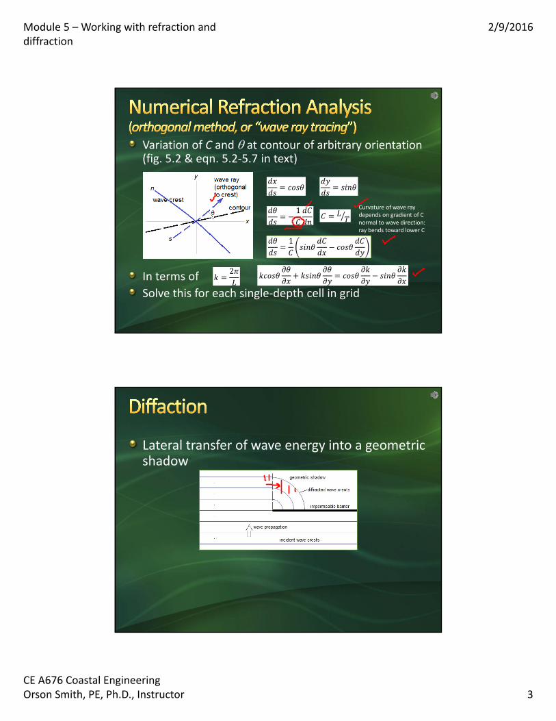
Figures in CEM Part II, Ch. 7, after Goda (2010)B/L = gap‐wavelength ratio
B
period height
Figures in CEM Part II, Ch. 7, after Goda (2010)B/L = gap‐wavelength ratio
period height ratio
Module 5 – Working with refraction and diffraction
2/9/2016
CE A676 Coastal EngineeringOrson Smith, PE, Ph.D., Instructor 6
Figures in CEM Part II, Ch. 7, after Goda (2010)B/L = gap‐wavelength ratio
Figures in CEM Part II, Ch. 7, after Goda (2010)B/L = gap‐wavelength ratio
Module 5 – Working with refraction and diffraction
2/9/2016
CE A676 Coastal EngineeringOrson Smith, PE, Ph.D., Instructor 7
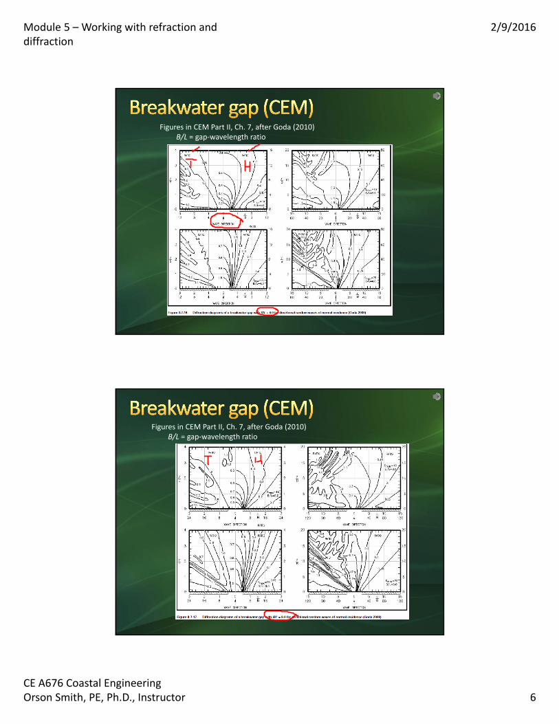
Rogue River entrance, Oregon
Coos Bay, Oregon
prevailing longshore sediment transport
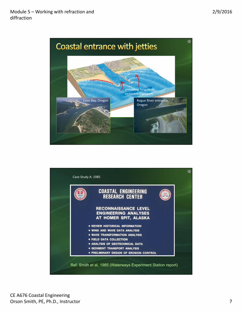
Ref. Smith et al, 1985 (Waterways Experiment Station report)
Case Study A: 1985

Module 5 – Working with refraction and diffraction
2/9/2016
CE A676 Coastal EngineeringOrson Smith, PE, Ph.D., Instructor 8

Module 5 – Working with refraction and diffraction
2/9/2016
CE A676 Coastal EngineeringOrson Smith, PE, Ph.D., Instructor 9

Module 5 – Working with refraction and diffraction
2/9/2016
CE A676 Coastal EngineeringOrson Smith, PE, Ph.D., Instructor 10
RCPWAVE numerical wave refraction, shoaling, and breaking model• Steady‐state, linear waves – monochromatic• No diffraction – open coast use only
Ref. Smith et al, 1985 (Waterways Experiment Station report)

Module 5 – Working with refraction and diffraction
2/9/2016
CE A676 Coastal EngineeringOrson Smith, PE, Ph.D., Instructor 11
Orson Smith, PE, Ph.D.Professor, UAA School of Engineering
Case Study B: 2002‐2003
Alexander Khokhlov, MS Candidate, Dept. of Civil Engineering, UAA School of Engineering
William J. Lee, Research Associate and Ph.D. candidate, Environmental Engineering Program, UAA School of Engineering
Steven Buchanan, RLS, Instructor, Dept. of Geomatics, UAA School of Engineering

Module 5 – Working with refraction and diffraction
2/9/2016
CE A676 Coastal EngineeringOrson Smith, PE, Ph.D., Instructor 12
Project Sponsors
Geomega, Inc. (Boulder, CO)
Chevron Environmental Management Company (San Ramon, CA)
Phase I Scope
Investigate geomorphologic change through history of the site and
survey data measured by UAA
Sample and classify beach materials
Characterize wave climate
Numerical simulations of nearshore wave transformation
Interpret geomorphologic changes with regard to local conditions

Module 5 – Working with refraction and diffraction
2/9/2016
CE A676 Coastal EngineeringOrson Smith, PE, Ph.D., Instructor 13
Rigtenders Dock
East Foreland
Mean Mean Spring Tide
North West Range Range Level Station Latitude Longitude (ft) (ft) (ft) Ushagat Island, Barren Islands 58° 57' 152° 16' 11.4 13.7 7.2 SELDOVIA, Kachemak Bay 59° 27' 151° 43' 15.5 18.0 9.4 Homer, Kachemak Bay 59° 38' 151° 27' 15.7 18.1 9.5 Anchor Point 59° 46' 151° 53' 15.9 18.3 9.6 Cape Ninilchik 60° 01' 151° 43' 16.5 19.1 10.1 Ninilchik 60° 03' 151° 40' 16.7 19.1 10.0 Kenai River entrance 60° 33' 151° 17' 17.7 20.7 11.0 Kenai City Pier 60° 33' 151° 14' 17.5 19.8 10.4 Nikiski 60° 41' 151° 24' 17.7 20.5 10.9East Foreland 60° 43' 151° 25' 18.0 21.0 11.2 Sunrise, Turnagain Arm 60° 54' 149° 26' 30.3 33.3 17.1 ANCHORAGE, Knik Arm 61° 14' 149° 53' 25.9 28.8 15.2 North Foreland 61° 03' 151° 10' 18.3 21.0 11.3 Drift River Terminal 60° 34' 152° 08' 15.4 18.1 9.7 Oil Bay, Kamishak Bay 59° 38' 153° 16' 12.6 13.9 7.3

Module 5 – Working with refraction and diffraction
2/9/2016
CE A676 Coastal EngineeringOrson Smith, PE, Ph.D., Instructor 14
Composite hourly dataKenai Airport (1973 ‐ 1997)
KPC Terminal, Nikiski (1997 ‐2002)
Radial scale is percent frequency of occurrence
Radial bands indicate 10‐knot wind speed classes acting toward the center
Wind rose analysis software and graphic by Josh Rogers, UAA School of Engineering
WindSpeed
Speedm/sec
Waveparameter
180 deg202.5deg
225 deg
247.5deg
270 deg
292.5deg
315 deg
0-9(5)
knots 2.57
H 0.16 0.17 0.17 0.16 0.14 0.13 0.14
T 1.56 1.77 1.70 1.55 1.43 1.34 1.39
10-19 (15)
knots 7.72
H 0.83 1.53 1.23 0.87 0.68 0.56 0.63
T 3.28 4.56 4.01 3.37 2.98 2.72 2.87
20-29 (25)
knots 12.86
H 1.43 3.19 2.32 1.64 1.28 1.06 1.18
T 4.35 6.43 5.48 4.55 4.01 3.64 3.86
30-39 (35)
knots 18.01
H 1.98 4.87 3.40 1.62
T 5.21 7.90 6.64 4.41
40-49 (45)
knots 23.15
H 2.49 6.56 4.45 2.66
T 5.94 9.16 7.64 5.60
50-59 (55)
knots 28.29
H 2.96 8.25 5.45
T 6.58 10.27 8.52
calculated using CEDAS – ACES wave prediction software ( Veri‐Tech, Inc.)

Module 5 – Working with refraction and diffraction
2/9/2016
CE A676 Coastal EngineeringOrson Smith, PE, Ph.D., Instructor 15
Extreme Waves Offshore of the Mouth of the Kenai River, 1973 - 2000
00.10.20.30.40.50.60.70.80.9
1
0 5 10 15 20 25 30
Wave Height, H' (ft)
Pro
bab
ilit
y o
f H
<H
'
Estimated Function
Data, 1973 - 2000
Extremal wave analysis by Heike Merkel from previous study sponsored by PN&D, Inc., and City of Kenai
Beach ice grows in upper tidelands and floats free to form sediment‐laden conglomerates
Average ice conditions 1‐15 February, showing color codes of concentration from 0 (no ice) to 10 tenths (100% ice cover) and hatch patterns to indicate stage of development (from Cook Inlet Ice Atlas by CRREL and UAA for NOAA, 2000)

Module 5 – Working with refraction and diffraction
2/9/2016
CE A676 Coastal EngineeringOrson Smith, PE, Ph.D., Instructor 16
Samples collected by Alexander Khokhlov
Analysis by Curtis Townsend, UAA Civil Engineering student
Sample No. 3, 4, 6, & 7
0
20
40
60
80
100
0.010.1110100
Grain Size , mm
Pe
rce
nt
Fin
er
#4: substrate below #3
#3: surface just north ofdock
#6: surface, just south ofopen-cell wall
#7: surface 40 ft offsouthern open-cell wall

Module 5 – Working with refraction and diffraction
2/9/2016
CE A676 Coastal EngineeringOrson Smith, PE, Ph.D., Instructor 17
#
#
#
#
#
#
##
#
#
#
110
100
90
80
70
60
50
4030 20 10
MLLW
13
12
11
10
9
7
6
5
3, 41, 2
8
586800
586800
587000
587000
587200
587200
587400
587400
587600
5876006728
600
672
8600
6728
800
6728
800
672
9000
6729000
672
9200
67292
00
672
940
0 6729400
672
9600
6729600
6729
800
672
9800
N
UTM Zone 5 (Meters)NAD 83
300 0 300
Feet
100 0 100
Meters
•Topographic survey: Steve Buchanan, RLS, Heike Merkel, Alissa Pempek, Josh Rogers, Alexander Khokhlov
•Hydrographic survey: Bill Lee, Alexander Khokhlov, Orson Smith
Low tide view of North inshore corner of Rigtenders Dock, July 2002.

Module 5 – Working with refraction and diffraction
2/9/2016
CE A676 Coastal EngineeringOrson Smith, PE, Ph.D., Instructor 18
Grid developed by Alexander Khokhlov and Bill Lee from NOAA archives and UAA 2002 survey data for STWAVE simulations
Steady‐state linear waves
Evolution of directional spectrumMultiple waves of different H, T, and Non‐linear transfer of energy within spectrum
Bottom friction, percolation, wind‐input, simple current interaction, breaking
Diffraction past simple structures

Module 5 – Working with refraction and diffraction
2/9/2016
CE A676 Coastal EngineeringOrson Smith, PE, Ph.D., Instructor 19
STWAVE output for Hs = 5.45 m, Tp = 9.09 sec, direction = 225° T (from southwest). Arrows are wave rays, contours are wave height, and colors are depths at mean tide level.
Climatic average condition: H = 0.6 m (2 ft), T = 4.2 sec, direction = 24 Northward
Beach barrier (Rigtenders Dock) blocks longshore transport from South

Module 5 – Working with refraction and diffraction
2/9/2016
CE A676 Coastal EngineeringOrson Smith, PE, Ph.D., Instructor 20
Offshore margin of Rigtenders Dock at low tide.

Module 5 – Working with refraction and diffraction
2/9/2016
CE A676 Coastal EngineeringOrson Smith, PE, Ph.D., Instructor 21
Phase II Scope
Extended numerical simulations
2nd topographic & hydrographic surveyQuantitative analysis of annual change
Wave measurementsEvaluation assumptions based on hindcast wave climatology
Discuss alternative engineering responses to erosion
Example BMAP analysis of profile change and of beach fill configurations
Example BMAP analysis of profile change and of beach fill configurations

Module 5 – Working with refraction and diffraction
2/9/2016
CE A676 Coastal EngineeringOrson Smith, PE, Ph.D., Instructor 22
Not For Navigational Use
Not Fo
N
EW
S
58°46'
58°52'
58°58'59°2'59°6'59°10'
59°16'
59°22'
59°28'
59°34'
59°40'
59°46'
59°52'
59°58'60°2'60°6'60°10'
60°16'
60°22'
60°28'
60°34'
60°40'
60°46'
60°52'
60°58'6
1°2'61°6'61°10'
61°16'
61°22'
154°48'
154°48'
154°36'
154°36'
154°24'
154°24'
154°12'
154°12'
154°00'
154°00'
153°48'
153°48'
153°36'
153°36'
153°24'
153°24'
153°12'
153°12'
153°00'
153°00'
152°48'
152°48'
152°36'
152°36'
152°24'
152°24'
152°12'
152°12'
152°00'
152°00'
151°48'
151°48'
151°36'
151°36'
151°24'
151°24'
151°12'
151°12'
151°00'
151°00'
150°48'
150°48'
15
15
Grid development by Alexander Khokhlov and Bill Lee, UAA/SOE
NOAA Chart 16660
NOAA Chart 16640

Module 5 – Working with refraction and diffraction
2/9/2016
CE A676 Coastal EngineeringOrson Smith, PE, Ph.D., Instructor 23
Module 5 – Working with refraction and diffraction
2/9/2016
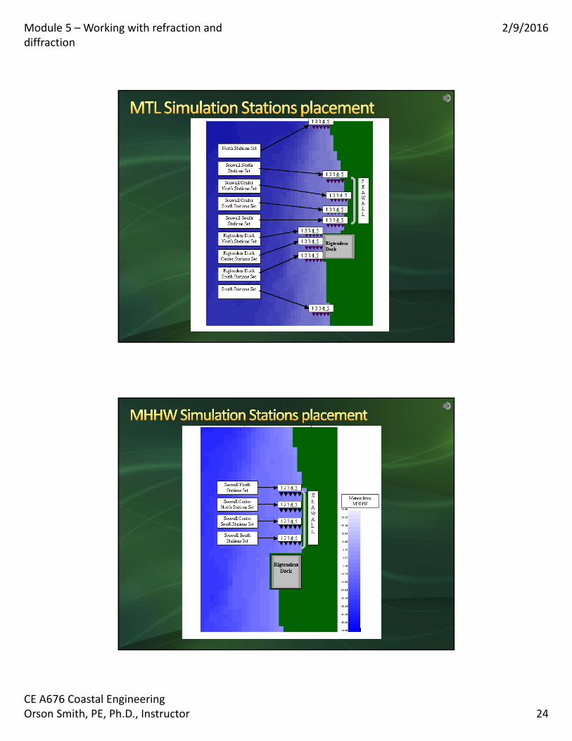
CE A676 Coastal EngineeringOrson Smith, PE, Ph.D., Instructor 24
Module 5 – Working with refraction and diffraction
2/9/2016
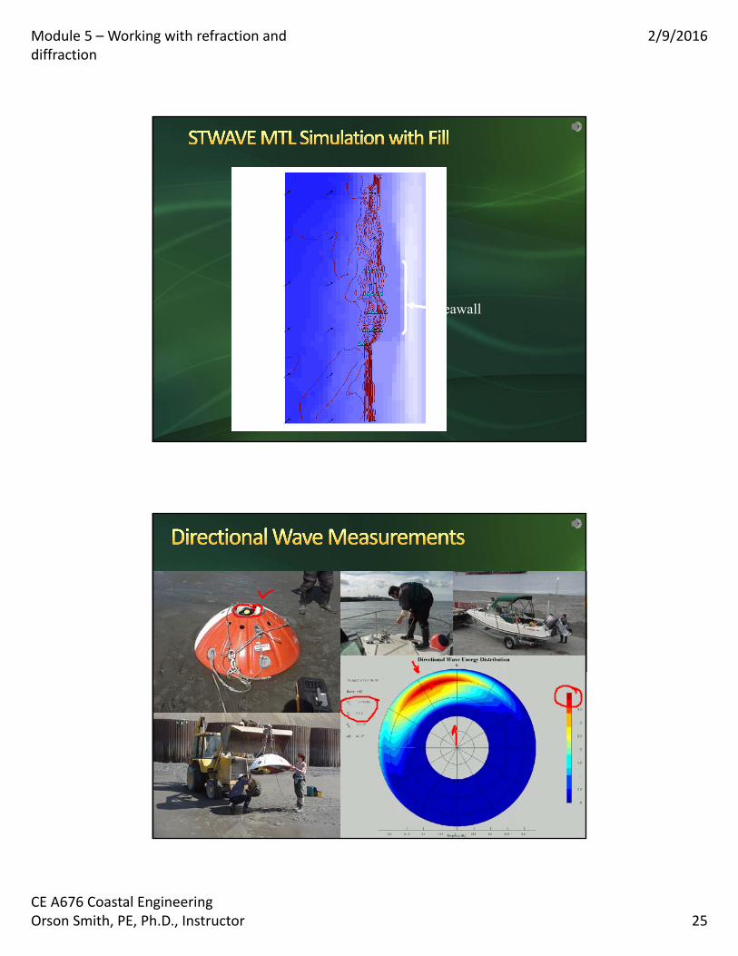
CE A676 Coastal EngineeringOrson Smith, PE, Ph.D., Instructor 25
Seawall

Module 5 – Working with refraction and diffraction
2/9/2016
CE A676 Coastal EngineeringOrson Smith, PE, Ph.D., Instructor 26
Data collected from 2003/06/09 13:36:40 to 2003/07/18 11:36:39
468 sea state measurements, 8.41 MB
Sample rate = 2 Hz, burst length = 1,024 seconds (2048 samples) every 2 hours
Spectral analysis:Frequency minimum = 0.04 Hz,
Ensemble average every 128 samples
Hanning‐type smoothing of ensembles
Wave height (from ADP data) and Wind speed (from NOAA database)Nikiski (06/09/2003 - 07/18/2003)
0
1
2
3
4
5
6
7
8
9
10
11
12
13
14
15
Date
6/10
/2003
6/11
/2003
6/12
/2003
6/13
/2003
6/14
/2003
6/14
/2003
6/15
/2003
6/16
/2003
6/17
/2003
6/18
/2003
6/19
/2003
6/20
/2003
6/21
/2003
6/22
/2003
6/23
/2003
6/24
/2003
6/25
/2003
6/25
/2003
6/26
/2003
6/27
/2003
6/28
/2003
6/29
/2003
6/30
/2003
7/1/
2003
7/2/
2003
7/3/
2003
7/4/
2003
7/5/
2003
7/6/
2003
7/6/
2003
7/7/
2003
7/8/
2003
7/9/
2003
7/10
/2003
7/11
/2003
7/12
/2003
7/13
/2003
7/14
/2003
7/15
/2003
7/16
/2003
7/17
/2003
7/17
/2003
Date
Win
d s
pee
d (
m/s
)
0
0.5
1
1.5
2
2.5
Wav
e h
eig
ht
(m)
Wind Speed (m/s) Wave Height (m)
Analysis and graph by Alexander Khokhlov, UAA/SOE

Module 5 – Working with refraction and diffraction
2/9/2016
CE A676 Coastal EngineeringOrson Smith, PE, Ph.D., Instructor 27