Stirling Engine for Solar Thermal Electric Generation · Solar thermal generation has had less...
106
Stirling Engine for Solar Thermal Electric Generation by Mike Miao He A dissertation submitted in partial satisfaction of the requirements for the degree of Doctor of Philosophy in Engineering – Electrical Engineering and Computer Sciences and the Designated Emphasis in Energy Science and Technology in the Graduate Division of the University of California, Berkeley Committee in charge: Professor Seth Sanders, Chair Professor Randy Katz Professor Dan Kammen Summer 2016
Transcript of Stirling Engine for Solar Thermal Electric Generation · Solar thermal generation has had less...

Stirling Engine for Solar Thermal Electric Generation
by
Mike Miao He
A dissertation submitted in partial satisfaction of the
requirements for the degree of
Doctor of Philosophy
in
Engineering – Electrical Engineering and Computer Sciences
and the Designated Emphasis
in
Energy Science and Technology
in the
Graduate Division
of the
University of California, Berkeley
Committee in charge:
Professor Seth Sanders, ChairProfessor Randy Katz
Professor Dan Kammen
Summer 2016

Stirling Engine for Solar Thermal Electric Generation
Copyright 2016by
Mike Miao He

1
Abstract
Stirling Engine for Solar Thermal Electric Generation
by
Mike Miao He
Doctor of Philosophy in Engineering – Electrical Engineering and Computer Sciences
University of California, Berkeley
Professor Seth Sanders, Chair
Addressing the challenge of climate change requires the large-scale development of sig-nificant renewable energy generation, but also requires these intermittent energy sources tobe balanced by energy storage or demand management to maintain a reliable electric grid.In addition, a centralized generation paradigm fails to capture and utilize thermal energyfor combined heat and power, abandoning a large portion of the available value from theprimary energy source. A solar thermal electric system utilizing Stirling engines for energyconversion solves both of these shortcomings and has the potential to be a key technology forrenewable energy generation. The ability to store thermal energy cheaply and easily allowsthe reliable generation of output power even during absences of solar input, and operatingas distributed generation allows the output thermal stream to be captured for local heat-ing applications. Such a system also can achieve relatively high conversion efficiencies, isfabricated using common and benign materials, and can utilize alternate sources of primaryenergy in an extended absence of solar input.
This dissertation discusses the design, fabrication, and testing of a Stirling engine as thekey component in a solar thermal electric system. In particular, the design addresses thelow temperature differential that is attainable with distributed solar with low concentrationratios and is designed for low cost to be competitive in the energy space. The dissertationcovers design, fabrication, and testing of a 2.5 kW Stirling Engine with a predicted thermal-to-mechanical efficiency of 20%, representing 60% of Carnot efficiency, operating between180 C and 30 C. The design process and choices of the core components of the engine arediscussed in detail, including heat exchangers, regenerator, pistons, and motor/alternator,and the process for modeling, simulation, and optimization in designing the engine. Finally,the dissertation covers the assembly and experimental testing that validates the design interms of heat exchanger performance, losses, kinematics, and cycle work.

i
To my wife, Michelle, for loving me and supporting me throughout my graduate career.

ii
Contents
Contents ii
List of Figures iii
List of Tables iv
1 Introduction 11.1 System Description . . . . . . . . . . . . . . . . . . . . . . . . . . . . . . . . 11.2 Stirling Engine Background . . . . . . . . . . . . . . . . . . . . . . . . . . . 2
2 Motivation 52.1 Broader Context . . . . . . . . . . . . . . . . . . . . . . . . . . . . . . . . . 52.2 Applications . . . . . . . . . . . . . . . . . . . . . . . . . . . . . . . . . . . . 11
3 Design and Optimization 213.1 Design Overview . . . . . . . . . . . . . . . . . . . . . . . . . . . . . . . . . 213.2 Analytical Design and Optimization . . . . . . . . . . . . . . . . . . . . . . . 223.3 Heat Exchangers . . . . . . . . . . . . . . . . . . . . . . . . . . . . . . . . . 233.4 Regenerator . . . . . . . . . . . . . . . . . . . . . . . . . . . . . . . . . . . . 323.5 Displacer Piston . . . . . . . . . . . . . . . . . . . . . . . . . . . . . . . . . . 343.6 Power Piston . . . . . . . . . . . . . . . . . . . . . . . . . . . . . . . . . . . 363.7 Adiabatic Simulation and Optimization . . . . . . . . . . . . . . . . . . . . . 393.8 Drive Train . . . . . . . . . . . . . . . . . . . . . . . . . . . . . . . . . . . . 463.9 Losses and Inefficiencies . . . . . . . . . . . . . . . . . . . . . . . . . . . . . 483.10 Pressurization . . . . . . . . . . . . . . . . . . . . . . . . . . . . . . . . . . . 563.11 Prototype Design . . . . . . . . . . . . . . . . . . . . . . . . . . . . . . . . . 59
4 Electrical Conversion and Motor Control 614.1 Alternator Design . . . . . . . . . . . . . . . . . . . . . . . . . . . . . . . . . 614.2 Drive Controls . . . . . . . . . . . . . . . . . . . . . . . . . . . . . . . . . . . 69
5 Experimental Results 805.1 Assembly and Verification . . . . . . . . . . . . . . . . . . . . . . . . . . . . 80

iii
5.2 Heat Exchanger Test . . . . . . . . . . . . . . . . . . . . . . . . . . . . . . . 815.3 Alternator Performance . . . . . . . . . . . . . . . . . . . . . . . . . . . . . . 855.4 Loss Experiments . . . . . . . . . . . . . . . . . . . . . . . . . . . . . . . . . 855.5 Forward and Reverse Operation . . . . . . . . . . . . . . . . . . . . . . . . . 88
6 Conclusion 946.1 Future Work . . . . . . . . . . . . . . . . . . . . . . . . . . . . . . . . . . . . 946.2 Final Words . . . . . . . . . . . . . . . . . . . . . . . . . . . . . . . . . . . . 94
Bibliography 96
List of Figures
1.1 System Diagram . . . . . . . . . . . . . . . . . . . . . . . . . . . . . . . . . . . 21.2 Ideal Stirling Cycle P-V Diagram . . . . . . . . . . . . . . . . . . . . . . . . . . 3
2.1 PV Installed Price . . . . . . . . . . . . . . . . . . . . . . . . . . . . . . . . . . 62.2 PV Cumulative and Annual Installed Capacity . . . . . . . . . . . . . . . . . . . 62.3 Diesel Cogeneration Payback . . . . . . . . . . . . . . . . . . . . . . . . . . . . 192.4 Diesel Cogeneration Market Segments . . . . . . . . . . . . . . . . . . . . . . . . 20
3.1 Top and bottom CAD view of heat exchanger body. . . . . . . . . . . . . . . . . 243.2 Heat Exchanger Complete View . . . . . . . . . . . . . . . . . . . . . . . . . . . 253.3 Working Fluid Channel Flow Simulation . . . . . . . . . . . . . . . . . . . . . . 283.4 Heat Exchanger External-Fluid Channel . . . . . . . . . . . . . . . . . . . . . . 303.5 Heat Exchanger External-Fluid Channel Structural FEA . . . . . . . . . . . . . 313.6 Displacer isometric and section view . . . . . . . . . . . . . . . . . . . . . . . . 343.7 Displacer deflection . . . . . . . . . . . . . . . . . . . . . . . . . . . . . . . . . . 363.8 Power piston isometric and section view. . . . . . . . . . . . . . . . . . . . . . . 373.9 P-V Diagram from Adiabatic Simulation . . . . . . . . . . . . . . . . . . . . . . 403.10 Optimization sweep over piston strokes . . . . . . . . . . . . . . . . . . . . . . . 423.11 Optimization sweep over regenerator stack length . . . . . . . . . . . . . . . . . 433.12 Working Fluid Stroke Length Sweep . . . . . . . . . . . . . . . . . . . . . . . . 453.13 Crankshaft Unconnected . . . . . . . . . . . . . . . . . . . . . . . . . . . . . . . 463.14 Crankshaft Assembled . . . . . . . . . . . . . . . . . . . . . . . . . . . . . . . . 473.15 Displacer linear bearing housing . . . . . . . . . . . . . . . . . . . . . . . . . . . 483.16 Assembled Engine with Wall . . . . . . . . . . . . . . . . . . . . . . . . . . . . . 57

iv
3.17 Pressure Vessel Drawing and Image . . . . . . . . . . . . . . . . . . . . . . . . . 583.18 Stirling Cycle Energy Flow Diagram . . . . . . . . . . . . . . . . . . . . . . . . 593.19 Engine Photographs . . . . . . . . . . . . . . . . . . . . . . . . . . . . . . . . . 60
4.1 Magnet rotor disc . . . . . . . . . . . . . . . . . . . . . . . . . . . . . . . . . . . 624.2 Assembled winding structure . . . . . . . . . . . . . . . . . . . . . . . . . . . . 634.3 Full rotor and stator assembly . . . . . . . . . . . . . . . . . . . . . . . . . . . . 644.4 Flux density versus rotor angle and fourier components . . . . . . . . . . . . . 654.5 Aspect Ratio Optimization . . . . . . . . . . . . . . . . . . . . . . . . . . . . . . 674.6 Normalized Aspect Ratio Optimization . . . . . . . . . . . . . . . . . . . . . . . 684.7 Custom Norm Level-Set . . . . . . . . . . . . . . . . . . . . . . . . . . . . . . . 754.8 Speed Control . . . . . . . . . . . . . . . . . . . . . . . . . . . . . . . . . . . . . 764.9 Control Block Diagram . . . . . . . . . . . . . . . . . . . . . . . . . . . . . . . . 774.10 Control Schematic . . . . . . . . . . . . . . . . . . . . . . . . . . . . . . . . . . 79
5.1 Engine Assembly Pictures . . . . . . . . . . . . . . . . . . . . . . . . . . . . . . 825.2 Electric Heater . . . . . . . . . . . . . . . . . . . . . . . . . . . . . . . . . . . . 835.3 Comparison of BackEmf from design and measurement . . . . . . . . . . . . . . 865.4 Spinning Losses Experiment Descriptions . . . . . . . . . . . . . . . . . . . . . . 875.5 Waveforms from Engine Test . . . . . . . . . . . . . . . . . . . . . . . . . . . . 905.6 PV Diagrams in Heat Pump mode . . . . . . . . . . . . . . . . . . . . . . . . . 915.7 PV Diagrams in Engine mode . . . . . . . . . . . . . . . . . . . . . . . . . . . . 92
List of Tables
2.1 Engine Capitol Costs . . . . . . . . . . . . . . . . . . . . . . . . . . . . . . . . . 142.2 Installed Price for Stirling vs PV . . . . . . . . . . . . . . . . . . . . . . . . . . 142.3 Full-Value Installed Price for Stirling vs PV . . . . . . . . . . . . . . . . . . . . 162.4 Diesel Generator Specifications . . . . . . . . . . . . . . . . . . . . . . . . . . . 17
3.1 Mesh longest path thermal resistances. . . . . . . . . . . . . . . . . . . . . . . . 263.2 Heat exchanger thermal resistances. . . . . . . . . . . . . . . . . . . . . . . . . . 293.3 Heat exchanger temperature drops. . . . . . . . . . . . . . . . . . . . . . . . . . 303.4 Important regenerator properties. . . . . . . . . . . . . . . . . . . . . . . . . . . 333.5 Displacer properties . . . . . . . . . . . . . . . . . . . . . . . . . . . . . . . . . 363.6 Power Piston properties . . . . . . . . . . . . . . . . . . . . . . . . . . . . . . . 39

v
3.7 Stirling engine losses . . . . . . . . . . . . . . . . . . . . . . . . . . . . . . . . . 453.8 Bearing Components . . . . . . . . . . . . . . . . . . . . . . . . . . . . . . . . . 483.9 Peak Piston Forces . . . . . . . . . . . . . . . . . . . . . . . . . . . . . . . . . . 483.10 Conduction path losses . . . . . . . . . . . . . . . . . . . . . . . . . . . . . . . . 503.11 Stirling engine losses . . . . . . . . . . . . . . . . . . . . . . . . . . . . . . . . . 543.12 Temperature drops . . . . . . . . . . . . . . . . . . . . . . . . . . . . . . . . . . 60
5.1 Heat exchanger conduction test temperature drops . . . . . . . . . . . . . . . . 835.2 Heat exchanger temperature drops. . . . . . . . . . . . . . . . . . . . . . . . . . 845.3 Heat Pump Equilibrium Thermal Test . . . . . . . . . . . . . . . . . . . . . . . 855.4 Heat Pump Equilibrium Thermal Test . . . . . . . . . . . . . . . . . . . . . . . 855.5 Spinning Losses Measurements and Predictions . . . . . . . . . . . . . . . . . . 875.6 Heat Pump Work . . . . . . . . . . . . . . . . . . . . . . . . . . . . . . . . . . . 935.7 Heat Pump and Engine Work Values . . . . . . . . . . . . . . . . . . . . . . . . 935.8 Combined Heat Pump and Engine Analysis . . . . . . . . . . . . . . . . . . . . 93

vi
Acknowledgments
I would like to thank Professor Seth Sanders for his mentorship and helping me to be abetter engineer, for his perpetual good humor and kindness, and for always being availablefor his students.
I would also like to thank Artin Der Minassians for his guidance and help. Thanks toAron, Matt, Roger, Sarah, and Shai on the Cleantech-to-Market team for their research onthe market viability of the technology. Thanks to Alan, Shong, Kelvin, Alex, and Samir andothers for their help.

1
Chapter 1
Introduction
Renewable energy is the cornerstone of humankind’s urgent endeavor to address the climatechange challenge on the technological front. The revolution of fossil energy enabled greatadvances in technology and society, but precipitated calamitous effects on the environment.To continue the pace of growth enabled thus far by plentiful energy, a new revolution willhave to be made toward clean and sustainable sources of power. Such a transition is theinevitable next step in the production of energy - the only question is the magnitude ofaccrued harm before it occurs.
To address this challenge, all forms of renewable energy should be explored and developed.Solar photovoltaic and wind power already have achieved a high profile and extraordinaryimprovements in cost and technology. Solar thermal generation has had less development andthe technology is less mature, despite possessing a set of potentially crucial advantages, suchas energy storage, combined heat and power, and potentially low-cost. This dissertation willdiscuss the design and development of a prototype Stirling engine for solar thermal energyconversion.
In this research, a full-power single phase Stirling engine prototype was designed, fab-ricated, and tested. This research builds on previous work in [22] on low-power single andmultiphase prototypes. The primary goals were to demonstrate the technical performanceand feasibility of this Stirling engine technology for use in commercial energy applicationsand to validate the design methodology to provide a path for future development.
1.1 System Description
The Stirling Engine is the central component of a distributed combined heat and powersystem envisioned in this research. The system as conceived is suitable for residential-scalepower generation and incorporates energy storage to produce consistent output power fromvariable solar resources. The rejected heat from the engine can be used for local heatingneeds, which further improves the total system efficiency.
A diagram of the solar thermal system is shown in Figure 1.1. The key components of

CHAPTER 1. INTRODUCTION 2
the system include a passive solar collector, a hot thermal storage subsystem, the Stirlingengine described herein, and an optional waste heat capture component. The system is de-signed with evacuated tube solar collectors in mind, as they provide the highest temperatureinput heat and efficiency of inexpensive commercially available collectors. The collectorsare non-tracking to reduce component count and lower cost, though passive concentratorswere added and tested to improve efficiency. Alternatively, on-site combustion can be usedas a thermal energy source in the absence of, or to balance, solar energy. The thermal en-ergy storage system can be realized with inexpensive hot water tanks that are commonlyused in residiential settings. Additional components include piping, fluid pumps, and heatexchangers for transferring heat between components and streams.
The majority of the system is designed to be composable from commercially availablecomponents to reduce cost and for simplicity. The exception to this is the Stirling engine,which requires significant engineering to achieve high performance at low cost. The Stirlingengine is the central component of the system and is the focus of this dissertation.
Figure 1.1: System Diagram
1.2 Stirling Engine Background
The Stirling engine is a heat engine that utilizes the Stirling Cycle to convert thermal energyflux into mechanical energy. The engine can also be run in reverse as a heat pump, whichcauses the inverse conversion. The Stirling Cycle is closed-cycle, which means that theinternal working fluid is retained and isolated from the external energy source. This thenrequires heat exchangers to transfer thermal energy from an external hot-side source intothe engine and from the engine to an external cold-side sink.

CHAPTER 1. INTRODUCTION 3
The Stirling Cycle is a thermodynamic cycle, and as such, is limited in efficiency by theCarnot Efficiency, given in Equation 1.1:
η = 1− TCTH
(1.1)
where η is the maximum theoretical efficiency, TC is the temperature of the cold-side reser-voir, and TH is the temperature of the hot-side reservoir.
As a gas cycle, the Stirling Cycle is usefully characterized by a P-V diagram, a plot ofthe internal pressure versus internal volume over a single cycle of the engine. An illustrativeP-V diagram is shown in Figure 1.2.
Figure 1.2: Ideal Stirling Cycle P-V Diagram
In the ideal P-V diagram, the trajectory of the engine is modeled as travelling along fourideal curves. These are shown in Figure 1.2 as a progression from point 1→ 2→ 3→ 4→ 1.

CHAPTER 1. INTRODUCTION 4
These four segments can be described as follows. 1→ 2 is an isometric (equal volume) stepwherein the enthalpy of the internal working fluid is increased by displacing gas through thehot-side heat exchanger and therefore imparting heat from the external high temperaturesource, all while keeping volume constant. The pressure increases during this step due tothe Ideal Gas Law. 2 → 3 is an isothermal expansion step wherein work is performedby expanding the internal working fluid, typically in a cylinder-piston subsystem. Thetemperature is kept constant by heat exchange with the high temperature source. 3→ 4 isanother isometric step wherein the enthalpy of the internal working fluid is descreased bydisplacing gas to the engine cold-side, while volume is kept constant. Finally, 4 → 1 is anisothermal contraction wherein work is performed on the internal working fluid to compressit, typically from the same piston that carried out the expansion earlier.
This represents a highly simplified and idealized description of the thermodynamic pro-cesses in a Stirling Cycle. In reality, several important deviations from the prior descriptionmust be noted. First, it is vastly more efficient to transfer the enthalpy of the working fluidto a regenerator in step 3 → 4, which is then returned to the working fluid in step 1 → 2.The regenerator is an important component of all real Stirling engines and is necessary forachieving high efficiency. Second, the discrete steps outlined are not traversed in disjointtimeframes, rather the real trajectory of the engine will simultaneously undergo two adjacentprocesses at each point in time. This leads to an actual P-V curve that resembles an inscribedellipse within the idealized curves shown in Figure 1.2. Third, the processes themselves arenot ideal; for example, there is no practical implementation of a truly isothermal process. Inreality, that step is more accurately modeled by an adiabatic process, wherein the enthalpyof the working fluid remains constant.
Given this description of the Stirling Cycle, the Stirling engine is then a mechanicalembodiment of the cycle. A Stirling engine can be realized in multiple different ways, butthe most common form includes two pistons, hot-side and cold-side chambers and heatexchangers, and a regenerator. One of the pistons is denoted the displacer piston, andis nominally responsible for driving the internal working fluid between the hot and coldchambers during the isometric steps. The other piston is denoted as the power piston, and isnominally responsible for the adiabatic expansion and compression of the working fluid. Thehot and cold chambers and heat exchangers serve to allow thermal flux between the workingfluid and the external hot and cold sources, respectively. The regenerator is responsible forrecapturing enthalpy during one part of the cycle and reimparting that enthalpy back to theworking fluid on the opposite half of the cycle. This configuration is a typical embodimentof a Stirling engine, and is in fact the configuration that was developed in this research. Itshould also be noted that an electric machine is required for conversion between the kineticenergy developed by the engine and electrical energy, and this component is also part of thisresearch.
A detailed discussion of the design and characterization of the components, loss terms,and non-idealities will be presented in Chapter 3.

5
Chapter 2
Motivation
This chapter will discuss the motivation behind this research into Stirling engines for ther-mal energy conversion. Additional context on renewable energy and energy storage will becovered, and then discuss potential benefits of this research on the field.
2.1 Broader Context
The endeavor of transforming the world’s energy portfolio from fossil-fuel generation torenewable generation in order to mitigate climate change is one of the biggest challenges of the21st century. Significant technological and societal advances will need to be made in additionto the extensive progress already achieved. Toward this goal, the Stirling engine systemproposed in this dissertation offers compelling advantages over many other technologies.
Over the past decade, renewable energy has undergone a period of rapid growth in tech-nology, cost-competitiveness, and production both domestically and worldwide. Not so longago, renewable energy was considered by many to be prohibitively expensive and impracticalas a bulk solution to clean energy. Since then, wind and solar energy have seen exponentialgrowth in installed capacity and continuous decline in prices. Solar photovoltaics are a com-pelling example, and are also the most direct comparison to the solar thermal technologyproposed herein.
The price of solar photovoltaics has plummeted in recent years, driven by a combinationof growth in silicon production from China, improvements in fabrication and installation ofpanels, and changes in business practices such as aggressive vertical integration in pursuit oflower costs. The median installed price of residential solar panels has dropped from $9.1/Win 2006 to about $4.3/W in 2014, and non-residential solar prices have dropped from $8.8/Win 2006 to $3.9/W for small systems (less than 500kW) and from $7.8/W to $2.8/W for largesystems (greater than 500kW) [3]. Over this same period of time, falling prices have spurredgrowth in annual installed capacity from about 110.8 MW in 2006 to about 2380.8 MW in2014 in the United States alone, with a domestic cumulative capacity of 9392.1 MW [3]. Eventhen, U.S. still ranks fourth in worldwide solar capacity, with Germany, Italy, and China

CHAPTER 2. MOTIVATION 6
leading. In 2014, worldwide installed capacity reached 178 GW, with 41 GW being added in2014 alone [26], and this growth shows no signs of slowing.
Figure 2.1: Solar photovoltaic installed price in the United States [3].
Figure 2.2: Solar photovoltaics annual and cumulative installed capacity by year in theUnited States since 1998 [3].
With the solar photovoltaic industry already expanding and maturing, it is necessary tomotivate the development of solar thermal energy as a compelling alternative technology.To that end, there are a number of fundamental technological advantages offered by solarthermal technology over solar photovoltaics, chief of which is the ability to easily store energy.The primary energy of renewable sources is fundamentally tied to intermittent and variableprocesses, such as sunlight and wind. As the installed capacity of such renewables grows, sodoes the degree of uncontrollable and unpredictable generation on the grid. The forthcoming

CHAPTER 2. MOTIVATION 7
need for energy storage has been widely recognized as a counterbalance to this increasingvariability. This energy storage can either come in the form of independent installationsof electrical storage systems, such as batteries and flywheels; or it can be derived fromdeveloping renewable energy sources that are inherently coupled with energy storage, suchas the Stirling engine solar thermal system.
Energy storage in a solar thermal system turns an unreliable resource into a reliable sourceof electricity, and does so at low cost, low complexity, and fully integrated into installation.Additionally, solar thermal also carries other important benefits, including the simplicity ofcomponents and conventionality of fabrication, which would aid in cost-competitiveness andbypassing production bottlenecks and supply chain issues; the potential for combined heatand power, which could significantly increase overall thermal efficiency; and application as adistributed generation system, fulfilling a role not available to technologies that rely on thescale of centralized installations. These motivations will be discussed in further detail.
Energy Storage
As renewable energy achieves higher penetration on the modern electric grid, the intermit-tency and variability in solar and wind energy become a more significant challenge thatmust be addressed by the industry. The underlying operation of the electric grid relies oninstantaneously fulfilling demand with regulated generation. The addition of large amountsof uncontrollable generation serves to break this contract, upending the way that the gridhas operated since the beginning. A certain amount of control must be present in the gridto maintain stability, so this gives rise to two fundamentally different but complementaryapproaches to integrating renewables.
The first is to add controllable compensation on the supply side in the form of energystorage or responsive fossil fuel generation. This addresses the challenge while serving tokeep the existing structure of supply-side control intact - good energy storage would beinvisible to the consumer. The second approach is to add controllability and responsivenessto the demand side of the grid. This has the advantage of utilizing the existing untappedflexibility of the demand side to perform the same function of balancing supply and demand,but challenges the entrenched paradigm of supply side control, and requires the introductionof pervasive intelligence and actuation on the demand side[11].
Most likely, both energy storage and controllable demand will be employed to aid in theprocess of renewable integration. The Stirling engine system as envisioned is potentially amixture of these two approaches. It incorporates energy storage to produce reliable powergeneration, but since it is a distributed system designed to be co-located with demand, itcan also autonomously balance load on the demand side. This carries advantages over eitherapproach employed independently - the storage available can balance both local generationand demand simultaneously. The technology is also attractive simply due to the fact thatit is generation with built-in storage. This enables grid integration with minimal effect ongrid stability.

CHAPTER 2. MOTIVATION 8
The energy storage potential of the Stirling engine system is a major compelling featurewhen compared to photovoltaic solar, and dramatically improves its competitiveness. Theoverall necessity for more storage is unequivocal and unambiguous in the industry, andit is quickly moving to incentivize and demand installation of storage. Examples includemandates for rapid expansion of energy storage capacities, such as California’s AB 2514,which as directed by the CPUC will mandate procurement of 1,325 MW of energy storagecapacity by the year 2020 [27], which almost doubles worldwide non-hydro storage [24] andis over 50 times California’s current installed storage capacity [25].
A Stirling-engine based thermal system contributes in two ways to the storage challenge.First, as a generation technology, its power output is reliable and consistent, presentingit as a technology that does not require additional balancing from storage. Indeed, it isflexible and controllable in its power output, both on short time scales of seconds by varyingthe frequency of the engine, or on longer time scales of minutes to hours by varying inputthermal energy. Second, the Stirling engine process is reversible, allowing it to be used asa pure energy storage mechanism by driving it in heat pump mode from grid energy, thenlater discharging stored energy in generation mode. In general, deriving a specific monetaryvalue from these advantages is difficult, depending on a number of factors including marketstructure, composition of generation sources, load profiles, and factors particular to a region.As a reference, NREL estimates that the value of electricity from a utility scale solar thermalis 2.57 times that of electricity from a solar photovoltaic plant given a 40% RenewablePortfolio Standard [15]. This comparison probably cannot be extrapolated directly to theStirling engine system, but points toward a significant value in reliable generation.
The energy storage market for non-hydro technologies is still relatively young and grow-ing. Energy storage mandates in the public sphere have been typically agnostic of tech-nologies, leaving room for a system such as the Stirling engine solar thermal system toparticipate. However, typical market structures do not easily accomodate or incentivizea distributed storage and generation technology such as this one. Renewable generation,such as photovoltaics, have mandated incentive structures, such as net metering, that donot provide additional incentives for the reliability of the source, hindering the ability of theconsumer to capture the value of storage. However, there are signs that this market structureis changing in recognition of the costs and challenges of the ever-growing share of renewablegeneration. For instance, PG&E is offering an incentive of up to $1.31/W for generationinstallations that have energy storage included [7]. Net metering programs have also facedsignificant challenges in recent years across multiple states, such as Nevada, Maine, Arizona,Hawaii, and California, partly as response to the hidden costs of providing a reliable gridwhen distributed PV is incentivized with retail electricity rates. A Stirling engine solar ther-mal system could alleviate some of these tensions between utilities and solar developers byintroducing ubiquitous energy storage along with the generation capacity.
One challenge is that monetization of the energy storage component of the Stirling enginesystem, apart from just providing firm capacity, is difficult in the current market structure.Energy storage is typically procured in the form of large centralized installations, and par-ticipates in markets in order to sell storage services such as regulation, load balancing, and

CHAPTER 2. MOTIVATION 9
reserves. Behind-the-meter energy storage is starting to gain some presence, especially sinceAB 2514, but is still in its infancy. Storage in the form of a Stirling engine system wouldhave a difficult time participating economically in energy markets in a consistent way acrossall service territories. As such, the economic value of energy storage from the proposedStirling engine system would be greatly enhanced if market structures were more universallysupportive of distributed storage. This does not diminish the value of research into sucha system, however, both in anticipation of market changes and for the intrinsic value fromdevelopment of a technically advantageous technology.
Combined Heat and Power
Combined heat and power refers to the generation of useful thermal energy in addition toelectricity. Combined heat and power enhances the value proposition from any particulartechnology by utilizing the thermal output of the system, an additional value stream thatis typically wasted or underutilized. It is particularly attractive for a thermal-based sys-tem, since conversion from thermal energy to electricity requires the rejection of heat asdetermined by the fundamental laws of thermodynamics.
The benefit derived from the supplementary thermal stream contributes to higher effi-ciency of the overall system by displacing energy otherwise needed for thermal services. Thisavoided energy use also provides another revenue stream and improves the economic propo-sition of the system. Accounting for the impact on efficiency of the supplementary thermalstream in CHP systems must be carefully done. There are in fact two measures of efficiencythat can be calculated - an overall system efficiency (thermal efficiency), and an effectiveelectrical efficiency. The two measures of efficiency have different uses. The overall systemefficiency is more straightforward and measures the fraction of useful energy produced versusthe energy consumed by the system. The effective electrical efficiency is useful to compare aCHP system with other forms of power generation without CHP. As a formula, the overallsystem efficiency is given by
ηO =WE +
∑QO
QI
(2.1)
where WE is the electrical power output of the system, QO are the useful thermal outputsof the system, and QI is the energy of the total thermal energy input. This measures thetotal useful output from the system compared to the energy input, and is well-suited forunderstanding how well the system makes use of its inputs.
The second measure of efficiency, the effective electrical efficiency, is given by the followingformula:
ηE =WE
QI −∑ QO
α
(2.2)
where WE is the electrical power output of the system, QO are the useful thermal outputsof the system, and QI , and α is the conversion efficiency of the displaced technology foreach usage of the thermal output. For example, α might be the efficiency of a water heater

CHAPTER 2. MOTIVATION 10
if the output thermal stream serves to heat water. This measure of efficiency accounts forthe value of the thermal stream as avoided input energy, taking into account the efficiencyof the avoided energy. Therefore, replacing an inefficient end-use of thermal energy is moreeffective than replacing an efficient one. This measure of efficiency is more useful for directcomparison with other forms of power generation, since it fully accounts for the differencesin energy usage due to avoidance between the forms of generation being compared.
Utilizing the thermal stream makes for a very favorable comparison between CHP ther-mal systems and other systems. For the particular system described herein, which has aconversion efficiency of 20%, these efficiency values can be calculated. If a very conservativeestimate is made that 50% of the rejected waste heat can be captured for water heating,this leads to a total system efficiency of 60%. Given that conventional water heaters areapproximately 80% - 90% efficient, this would lead to an effective electrical efficiency of 36%- 40%, a value that is significantly better than other renewable technologies and competitivewith centralized power generation.
Distributed Generation
Distributed generation is an area with a high potential of growth. By 2020, installed capac-ity of distributed generation is predicted to reach 15 to 20 GW [5]. Distributed generationconveys several important advantages as well as disadvantages versus centralized power gen-eration. These advantages include the ability to use rejected heat for onsite CHP, reductionin transmission and distribution losses and capacity, and microgrid or islanding capability.The chief disadvantage is the possibility of poor scaling of the technology down to smallscale and the lack of economies of scale with respect to manufacturing and deployment. Ap-plied to Stirling engine technology, however, the advantages are highly relevant, while thedisadvantages are less adverse, leading these considerations to favor distributed generationfor this technology.
Centralized power generation is highly limited in its ability to utilize rejected heat, dueto the fact that large power plants are typically not co-located with demand for thermalenergy. This energy stream is almost always simply dissipated to the environment, and fur-thermore is dissipated by consuming large quantities of water. According to [17], electricitygeneration in 2012 in the United States produced 12.4 Quad of electricity for 25.7 Quad ofrejected heat, representing an overall system efficiency of only 32.5%.. If this thermal energycould be utilized in a consistent manner, the overall system efficiency of electric generationcould be dramatically improved. This is one of the most important rationale for distributedgeneration. However, certain technologies are better suited than others for combined heatand power. Since the Stirling engine is a heat engine, it fundamentally must reject heat inorder to generate work according to the laws of thermodynamics. This heat is also typicallyrejected via a thermal fluid stream, rather than dissipatively to the environment. This makesit a good candidate for combined heat and power, especially at the lower input temperaturesthat are targeted by this project, which necessitate a higher fraction of rejected heat.

CHAPTER 2. MOTIVATION 11
The second major advantage of distributed generation is that transmission of power isobviated. This both reduces losses due to transmission inefficiencies and reduces the load onthe transmission system. According to the U.S. Energy Information Administration [1], 7%of transmitted energy is lost due to the transmission and distribution system. Distributedgeneration does not incur this penalty. Perhaps more importantly, expansion of utility-scale intermittent renewable energy will add significantly to transmission and distributionrequirements. Capacity of the T&D system must be sized for peak power, not averagepower, which leads to poor utilization of the capital investment in the grid. The energystorage capabilities of the Stirling engine system help to reduce this burden on transmissionand distribution - a controllable and reliable generation source requires less power transferfrom the grid than a source that adds to variability. Energy storage also aids in microgridor islanding capabilities - when there is no stable grid, a generation source with reliablepower is extremely beneficial. The alternative is to install fuel-based generation or expensivestandalone energy storage systems, such as batteries, to provide reliability.
The main disadvantages of distributed generation are due to scaling. Many technologies,including Rankine cycle or Brayton cycle machines, scale very well upwards, with largermachine size, but scale poorly down to smaller machine sizes. The opposite tends to be truefor Stirling engines - they operate at relatively high efficiencies at smaller scales correspondingto distributed generation levels, but do not scale to larger sizes as well. This is primarilydue to the difficulty of delivering thermal energy through a heat exchanger as length scalesare increased. Note that this scaling discussion refers to changing efficiencies at differentpower levels for a single machine; Stirling engines could certainly be combined in parallel toachieve higher total power ratings instead of increasing the size of a machine, but this simplyscales power linearly and does not improve the overall efficiency in fundamental ways. Atechnical discussion of scaling of Stirling engines is given in Section 3.9. In contrast, Braytonor Rankine cycles are more efficient as the engine size is scaled up. Therefore, the size andpower levels of distributed generation tend to play towards a strength of Stirling generation,namely better efficiency at smaller scales.
Distributed generation is furthermore better suited for electrification in the developingworld, compared to large-scale centralized power. In many places, long distance transmissionand distribution systems are in poor quality or non-existent, and development of significantT&D capability can be prohibitively expensive. In these cases, distributed generation withinmicrogrids presents a more likely path forward for electrification. Generation units on thescale of a few homes to small neighborhoods are well-suited for these purposes.
2.2 Applications
The Stirling engine’s flexibility with respect to thermal input allows the technology to bereadily used for multiple types of applications. This section will discuss specific applicationsand how the previously outlined advantages contribute to the value of the system. Certaincombinations of applications can be fulfilled with a single design, though others require a

CHAPTER 2. MOTIVATION 12
certain amount of redesign and sacrifices to achieve high performance. Two of the mostpromising applications for the technology will be covered - distributed generation and dieselcogeneration - along with prospects for commercialization and additional design considera-tions for these applications. Since Stirling engine technology is relatively sparse in most ofthese application spaces, the discussion is necessarily somewhat speculative.
Distributed solar generation
The original intended application for the Stirling engine system was distributed solar genera-tion. The primary competing technology in this space is rooftop photovoltaics. Photovoltaictechnology has major commercial advantages in the forms of industry adoption, manufac-turing infrastructure, public familiarity, targeted financing programs, and low cost throughmaturation on a learning curve. It also has major technical advantages including the sim-plicity of the technology compared to Stirling - in particular, the absence of plumbing andheat exchangers - and the potential for higher electrical conversion efficiency. These aresteep advantages to overcome if distributed Stirling systems are to achieve penetration inthe same market segment.
The proposition for Stirling systems in this application space therefore presumes two keyfactors - that energy storage and combined heat and power will become important advanta-geous features. As discussed previously, energy storage may become an important enablerand prerequisite for high levels of renewable generation from intermittent primary energysources. This may manifest concretely in the form of regulations or financial incentives thatpromote energy storage with distributed generation. Additionally, there may be consumerdemand for reliable renewable power for certain customers or end-uses. The ability to fullypower one’s home without drawing from the grid, including during cloudy weather or atnight, can be an appealing feature. Industrial or commercial facilities that wish to em-ploy renewable energy may find reliable generation sources much more appealing for criticalapplications, or for financial reasons like avoiding high demand charges. Possibly more im-portantly, the ability to generate reliable power is extremely relevant to electrification in thedeveloping world.
Likewise, the combined heat and power capabilities of the Stirling system add value bydisplacing a certain amount of thermal energy consumption, such as natural gas heating.This could allow users to fully supply their energy needs without purchasing any energyservices from a utility, given proper design and sizing of the system components for theparticular building. Two considerations should be noted. The first is that the ratio ofthermal output to electric output of the Stirling system is typically higher than the ratio ofthermal demand to electric demand in a typical modern U.S. household. [23] Excess thermaloutput can also be more effectively utilized by redesigning certain energy services. Heat canbe used for cooling and refrigeration by use of absorption chillers, for example. The secondis that thermal energy demand can vary greatly based on climate; such a system may bewell suited to particular locations and seasons but poorly suited to others.

CHAPTER 2. MOTIVATION 13
Though PV systems can have battery storage systems installed, this is typically pro-hibitively costly, especially on a distributed scale. For combined heat and power, PV systemscan be fitted with heat capture technology, which also serves to improve the performance ofthe PV cells by lowering their temperature. [23] However, this adds additional cost, and thequality and quantity of thermal energy recoverable is not comparable to Stirling engine sys-tem. To offer the complete feature set that the Stirling engine system offers, PV systems losetheir cost-competitiveness while still not equaling Stirling systems in each area. However,it is important to point out that the two technologies are not mutually exclusive; Stirlingsystems may cover important niches where energy storage and thermal output are valuablefeatures, while photovoltaics continue to dominate in more typical applications.
Central to the market potential of the Stirling engine system is its cost. Since a full-scale prototype was fabricted in the course of this project, a final production cost for theengine and system can be predicted with a reasonable amount of accuracy. This is based ona combination of costs for commercially available components and predictions for costs ofcustom-machined components at higher production quantities. To determine the economicviability of the Stirling engine technology, the costs and price of the 2.5 kW system wereevaluated. Table 2.1 lists component prices for manufacturing the Stirling engine at moder-ate scale. For commercially-available components, costs are taken by averaging the top 10vendors for that component. For custom machined components, the costs are quoted frommachine shops. The balance of system is estimated at 40% of total engine cost, a typicalvalue for this type of machine. A 30% margin is also accounted for, given by the industrypractice for small generators or turbines. This gives the final price of $3.10/W for the 2.5 kWengine.
The Stirling engine must be compared to a comparable distributed photovoltaic sys-tem to gain insight into its market competitiveness. Table 2.2 gives a comparison betweendistributed Stirling generation, as laid out in this dissertation, compared to distributed pho-tovoltaic generation. The capital price of the Stirling system from Table 2.1 is entered on thefirst line in this table. The price of PV panels listed is the 2014 median price for installationsunder 10 kW [3]. Additionally, the Stirling system requires the purchase of commercially-available evacuated tube collectors, which has been priced at $0.70/W by directly talkingto suppliers. This component does not apply to PV panels, which perform both functionsof collection and conversion. PV installations have both a module-price component, whichis listed in the first line, and non-module balance of system prices. The balance of systemincludes inverters, mounting hardware, labor, permitting and fees, overhead, taxes, and in-staller profit. The balance of system costs for the Stirling engine system are remarkablysimilar - each of these components are likewise necessary. The installation of collectors onthe rooftop is parallel to the installation of the PV panels themselves. Additionally, theinstallation of the engine itself, along with plumbing, storage tanks, and pumps are neces-sary for the Stirling engine. These additional costs were included in the price of the enginepreviously, in Table 2.1. Therefore, balance of system costs for PV installations are goodproxies for the remaining balance of system for Stirling systems, and are assumed to be thesame in this analysis.

CHAPTER 2. MOTIVATION 14
Hardware Components Cost per engine $ per watt
Alternator $245
Crankshaft $250
Piston Lubrication $10
Heat Exchanger Mesh $50
Custom Machined Components $1372
Other Components $1400
Assembly (20hrs $20/hr) $400
Shipping $30
Pressure Vessel $500
Engine Total $4257 $1.70
Balance of System $0.70
30% margin $0.70
Final Price $3.10
Table 2.1: Breakdown of engine capital costs for Stirling engine converter [16].
Component Stirling Engine Distributed PV [3]
Engine System $3.10/W $0.70/W
Collector $0.70/W
Balance of System $3.60/W $3.60/W
Total $7.40/W $4.30/W
Table 2.2: Installed price comparison between distributed Stirling system and distributedPV system [3]. Balance of System includes all non-module prices in an installation, and isassumed to be the same between the systems.

CHAPTER 2. MOTIVATION 15
As can be seen in this table, the Stirling engine system is not cost competitive withmodern distributed photovoltaic systems on this basis alone. In 2006, at the beginning ofthis project, distributed solar PV module prices were approximately $4/W, leading to ainstalled cost of $8.60/W. This made for a much more favorable comparison, especially withthe additional benefits of energy storage and combined heat and power. Additionally, PVis continuing its aggressive reduction in prices year after year. For example, from 2011 to2012, installed PV prices fell by $0.90/W (14%). As it stands currently, the Stirling enginesystem is not a viable competitor for direct generation on this basis. However, this is methodof comparison does not capture all the value streams in a Stirling engine, since the Stirlingsystem is more feature rich than the PV system, incorporating CHP and energy storage.
A more favorable, and more technologically even, comparison is given by including thebenefits from energy storage and CHP. Energy storage can be accounted for by includingthe price of a commensurate battery storage system with the price of the PV system. Thebattery system is sized to be equivalent to the storage in a representative design of theStirling engine, providing 4 hours of storage, a modest level of storage. Battery prices varywidely based on chemistry, manufacturing, and usage. There is no consensus cost for aresidential battery storage system, given that it is still a niche product. As a representativenumber, SolarCity has made potentially the most competitive play for residential batterystorage and has priced its system at $2000 kW−1 h [14]. With 4 hours of storage as thecomparison point, this equates to an additional cost of $8/W. Storage in the Stirling enginesystem requires only additional storage tanks, up to the quantity of storage desired, and apump with controller. Most of the other necessary components are already included in thebase Stirling system. These components only add minimal cost to the system for additionalstorage.
To account for the benefit from CHP, the value of the thermal stream must be determinedalong with an equivalent electrical value. The most direct comparison is to account forthe energy displaced by the thermal stream, including the conversion efficiency of energydisplaced. Fortunately, this is precisely what the effective electrical efficiency for a CHPsystem measures, as discussed in Section 2.1. In this accounting, the effective efficiencyof the Stirling converter becomes approximately 36% if the thermal stream is used for aubiquitous application such as water heating. This effectively increases the rated capacityof the system, and lowers the $ per watt inversely proportionally by the same amount.Accounting for these storage and CHP value streams in the Stirling engine system, a newcomparison can be made, as show in in Table 2.3.
The Stirling engine solar thermal system has a major advantage when the full cost ofenergy storage is included in a photovoltaic system. There are additional factors that favorthe Stirling engine. Battery storage systems have a shorter cycle lifetime than thermalstorage tanks, and must be replaced at some point in the lifetime of the system, addingNPV cost. This comparison is made based on 4 hours of storage, a small quantity sufficientfor basic energy shifting of peak solar input times to peak demand times. If storage capacitywere expanded to cover a full day, the calculus is even more in favor of the Stirling engine,since per-kWh costs for thermal storage are far less than for batteries. This level of storage

CHAPTER 2. MOTIVATION 16
Component Stirling Engine Distributed PV [3]
Engine System $3.10/W $0.70/W
Collector $0.70/W
Energy Storage $0.50/W $8.00/W
Balance of System $3.60/W $3.60/W
Total $7.9/W $12.30/W
Table 2.3: Installed price comparison between distributed Stirling system and distributedPV system, accounting for the full value of CHP and energy storage. Energy storage isaccounted for by additional battery storage in the PV system while CHP is accounted forby using the effective electrical efficiency of the Stirling engine.
might be desirable for microgrids for long duration islanding capability.The main barrier to realizing this advantage in this application space is the lack of a
market structure to fully incentivize the energy storage. A more likely path forward forStirling engine technology used as distributed generation is in the developing world. Inparticular, the advantages of Stirling engines in CHP and energy storage are well-suited formicrogrids or off-grid applications. Here, built-in energy storage presents itself as especiallyappealing without stable or reliable central grids to connect to. The installation of batterieswith PV as an alternative energy storage mechanism is not as attractive, due to the difficultyof manufacturing and disposal of batteries and the complexity of electrical hardware andcontrols. Thermal energy storage for the Stirling engine, on the other hand, is decidedlylow-tech and simple to implement, taking the form of storage tanks, pipes and pumps.The thermal output of the engine is also potentially highly useful for water heating wherealternatives like gas heating may not have existing infrastructure. Additionally, the fuelflexibility of Stirling engines enables the use of fuel as supplementary or backup energy,adding further flexibilty and reliability in its utilization. This is an area where the strengths ofthis technology may be valuable enough to overcome the basic cost advantage of photovoltaictechnology.
Waste Heat Capture
Waste heat capture is another important application space for Stirling engines. The termencompasses a very broad spectrum of possible applications, with sometimes very differentrequirements and characteristics, different waste heat temperatures, power quantities, andambient constraints. Some examples of potential applications include capturing industrialwaste heat byproducts, as a bottoming cycle for other generation systems, and capturingotherwise unusable energy at remote sites such as offshore oil wells. Since the applicationspace is so broad, it is difficult to characterize the applicability of Stirling engines in a general
CHAPTER 2. MOTIVATION 17
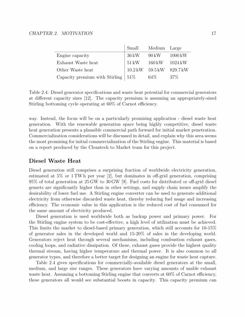
Small Medium Large
Engine capacity 36 kW 90 kW 1000 kW
Exhaust Waste heat 51 kW 160 kW 1024 kW
Other Waste heat 10.2 kW 59.5 kW 829.7 kW
Capacity premium with Stirling 51% 64% 37%
Table 2.4: Diesel generator specifications and waste heat potential for commercial generatorsat different capacity sizes [12]. The capacity premium is assuming an appropriately-sizedStirling bottoming cycle operating at 60% of Carnot efficiency.
way. Instead, the focus will be on a particularly promising application - diesel waste heatgeneration. With the renewable generation space being highly competitive, diesel wasteheat generation presents a plausible commercial path forward for initial market penetration.Commercialization considerations will be discussed in detail, and explain why this area seemsthe most promising for initial commercialization of the Stirling engine. This material is basedon a report produced by the Cleantech to Market team for this project.
Diesel Waste Heat
Diesel generation still comprises a surprising fraction of worldwide electricity generation,estimated at 5% or 1 TW h per year [2], but dominates in off-grid generation, comprising95% of total generation at 25 GW to 30 GW [9]. Fuel costs for distributed or off-grid dieselgensets are significantly higher than in other settings, and supply chain issues amplify thedesirability of lower fuel use. A Stirling engine converter can be used to generate additionalelectricity from otherwise discarded waste heat, thereby reducing fuel usage and increasingefficiency. The economic value in this application is the reduced cost of fuel consumed forthe same amount of electricity produced.
Diesel generation is used worldwide both as backup power and primary power. Forthe Stirling engine system to be cost-effective, a high level of utilization must be achieved.This limits the market to diesel-based primary generation, which still accounts for 10-15%of generator sales in the developed world and 15-20% of sales in the developing world.Generators reject heat through several mechanisms, including combustion exhaust gases,cooling loops, and radiative dissipation. Of these, exhaust gases provide the highest qualitythermal stream, having higher temperature and thermal power. It is also common to allgenerator types, and therefore a better target for designing an engine for waste heat capture.
Table 2.4 gives specifications for commercially-available diesel generators at the small,medium, and large size ranges. These generators have varying amounts of usable exhaustwaste heat. Assuming a bottoming Stirling engine that converts at 60% of Carnot efficiency,these generators all would see substantial boosts in capacity. This capacity premium can

CHAPTER 2. MOTIVATION 18
equivalently be translated into reduced fuel use - the advantage provided by the Stirlingengine can be designated on a continuum from lowered fuel usage at a constant capacityrating to higher capacity rating at a constant fuel usage.
The economic value of the Stirling engine co-system is heavily influenced by the cost ofthe diesel fuel. The range of applications and corresponding fuel prices is wide - in the UnitedStates and other highly-developed countries, the cost of diesel fuel is approximately $1 L−1;in developing countries, the cost of diesel is double that at $2 L−1; and in remote or supply-chain-sensitive applications such as military installations, the cost of disel is over $5 L−1
[4]. Based on these prices, Figure 2.3 shows payback periods in each of these applications,with additional sensitivity analysis for scenarios where the Stirling engine final price is $2/W,$3/W, and $6/W. These payback periods were calculated assuming 20 hours of operation perday, which is appropriate for diesel used as prime power. The Levelized-Cost-of-Electricitylisted in the Figure is derived by calculating the marginal cost of electricity produced byinstalling the Stirling engine.
The base case price of the Stirling engine is projected to be $3/W, as seen previouslyin Table 2.1. However, for a full understanding of market risk, the sensitivity analysisat the lower and higher price points is highly important. The base case predicted price iscalculated given the best available knowledge at this point, but could easily be higher becauseof unforeseen design modifications, supply chain problems, or legal or regulatory issues.Likewise, the price could come in lower due to advancements in design or manufacturingprocesses. Therefore, included in the payback analysis are scenarios for 33% reduction inprice, at $5/W, and doubled price, at $6/W. It should be noted that the base case costanalysis ($3/W) discussed previously in the context of distributed generation is actually, bydesign, specified fully-configured for diesel cogeneration - it includes the engine itself as wellas plumbing, balance of system, and installation of the engine that is appropriate for bothapplications. Costs that are particular to distributed solar generation were included anddiscussed separately.
As can be seen in Figure 2.3, payback period at $3/W is very attractive over the rangeof diesel prices. In high-end military applications, the payback period is a short 4 monthslong, and even for mundane developing world applications, the payback period is about ayear and a half. Even if Stirling engine prices were double the projected value, at $6/W, thepayback period is still highly competetive at 7 months for military applications and threeyears for developing world applications. Even the worst case in this set of scenarios, with apayback of three years, is compelling in economic terms.
Besides cost effectiveness, the other necessary component of profitability is sufficientmarket size. The space of this application is already limited to prime diesel cogeneration.However, this sector represents a reasonably large market segment. As shown in Figure 2.4,even limiting the space to high-end applications where the cost of diesel fuel is high enablesa market size of roughly $2.5 billion. This figure shows the various market segments forthis type of Stirling application, organized by the cost of diesel fuel and the barrier to entryin that market. Different market segments are scaled by available market size. The primeapplications are therefore military and off-grid telecom, represented at $800 million and $1.5

CHAPTER 2. MOTIVATION 19
Figure 2.3: Payback periods associated with Stirling engine diesel cogeneration in differentmarkets, with sensitivty to price per watt included.
billion, respectively. For military applications, reduction of diesel fuel usage is especiallyattractive, as the fully-burdened cost of fuel reaches $100 L−1 [8]. Microgrids are also anappealing area for second-phase growth. Once commercial and manufacturing infrastruc-ture for the technology has been established, further expansion into grid applications orcommercial microgrids is available.
Summary
In this chapter, the current state of renewable energy was discussed in order to providecontext for and to motivate the development of the Stirling engine solar thermal system.It is imperative to transform the electric grid to one based on clean, renewable generationto address the environmental challenges of modern civilization. With such a change, theimpending need for storage and reliability that accompanies the growth of intermittent gen-eration poses a deep challenge that solar thermal systems, such as the one proposed hereinthis disseration, are uniquely poised to address. The technological and economic advantageswere discussed and shown to be highly compelling, given the proper market structure andincentives. In particular, two applications have been covered which hold the greatest poten-tial: distributed generation and waste heat recovery. These application areas are selectedfor technological and economic competitivness and are the most likely path forward for thetechnology.

CHAPTER 2. MOTIVATION 20
Figure 2.4: Market segments for the Stirling engine as prime diesel cogeneration, organizedaccording to cost of diesel fuel and barrier to entry [16].
The rest of the dissertation will discuss the technical details of the design, development,and testing of the prototype Stirling engine that forms the central component of the overallsystem. This research serves to demonstrate the technological basis for the Stirling enginesystem as a promising piece of the renewable energy revolution.

21
Chapter 3
Design and Optimization
This chapter will cover the detailed design of the Stirling engine converter. The goal is tocreate a design for a Stirling engine that can operate at relatively high efficiency at a lowsystem cost, while remaining simple to fabricate. This work builds on previous work in[22], while targeting much higher power levels and expanding that work with more detailedphysical models and design procedures. The design process incorporates models from mul-tiple physical disciplines, such as heat exchanger analysis, fluid flow models, and kinematicsimulations, and also utilizes different methods of analysis, such as static model-based char-acterization, dynamic simulation, and system-wide parameter optimization. This chaptercovers the mechanical portion of the design; electrical conversion and control will be coveredin Chapter 4.
3.1 Design Overview
An extensive effort was performed to optimally design a Stirling engine for its intendedapplication. This process consisted both of numerical analysis and optimization as well asmechanical design with considerations toward cost-effectiveness and practicality. In partic-ular, extensive design is needed in order to achieve good performance while meeting theimportant constraints of low input-temperature and low-cost. These factors differentiate theStirling engine in question from the typical modern Stirling engine. As will be seen, thedesign and optimization process leads to an engine with a considerably different physicalconfiguration.
The use of solar collectors with no concentration or low concentration means that inputtemperature to the Stirling engine can realistically only reach approximately 200 C. Thispresents the most significant constraint and challenge to the design of the engine. TypicalStirling engines can utilize input temperatures in the range of 300 C to 500 C from primaryenergy sources such as fuel combustion and radio-isotopes. Lower input temperatures implya lower maximal Carnot efficiency, but in addition imply that sources of loss or inefficiencyare all relatively more detrimental to the overall performance of the engine. Temperature

CHAPTER 3. DESIGN AND OPTIMIZATION 22
drops across heat exchangers use up a much greater fraction of the available exergy of theinput heat, and losses such as friction and compression loss comprise a larger fraction of theoverall available work output. Thus, the design of a Stirling engine under these conditionsleads to an exceptional effort to reduce losses, even at the expense of lower power rating.
The cost-competitiveness of the energy generation application space also places stringentrequirements on the system. This requires the modification of several important Stirlingengine standbys. Exotic materials are often used for the hot-side heat exchanger, such asInconel for its strength and corrosion resistance at high temperatures, but add significantlyto engine cost. A very different approach has been taken with the heat exchanger in thisengine. The regenerator of a Stirling engine - one of the most important components interms of conversion efficiency - is usually engineered for very high performance but is one ofthe costliest components. However, a different approach must be taken in the design of thisengine in the pursuit of low cost. The regenerator instead is optimized for high performancewith low-cost materials. The details of these components and optimization will be discussed.
In addition to careful design of individual components, comprehensive holistic design ofthe engine must be performed. Different components in a Stirling engine are remarkablyinterdependent and interconnected. Modifications to the heat exchanger design can greatlyimpact the optimal motion of the displacer piston, for example. This is due in part to thefact that the Stirling engine is a tightly packaged, enclosed system with a working fluid thatmoves through the components repeatedly over each cycle. The components must also bedesigned to fit together well physically, as excess dead space reduces developed pressure, andexcess material increases thermal losses and cost.
The rest of the chapter will cover the process of analysis and optimization, details ofspecific components, design choices and tradeoffs, and the mechanical design through CADdrawings and component specifications.
3.2 Analytical Design and Optimization
A detailed analytical multi-physical model was written that spanned all the important com-ponents in the Stirling engine. This model was designed to predict as accurately as possiblethe performance of a Stirling engine design, and drew upon previous experience in Stirlingengines and well-established research or domain knowledge on characteristics such as thermaltransfer, losses, mechanical behaviors, etc. By incorporating these disparate elements intoa unified design package, an end-to-end design is enabled that can achieve the performancedesired for the intended application.
The Stirling engine design procedure can be categorized into three steps of evaluation,each taking the previous as input: analytical models of a variety of components or physicalbehaviors of the engine, such as heat exchangers, fluid flows, and other losses; an adiabaticdynamic simulation to evaluate the thermodynamic cycle performance of the engine; finally,an optimization step to guide design parameters for improving the design. The optimizationstep was used to improve the set of easily-adjustable design parameters for each evaluation,

CHAPTER 3. DESIGN AND OPTIMIZATION 23
but significant modal changes, such as evaluating the engine for an entirely different workingfluid, required separate runs of the procedure. These three steps were run over a variety ofinteresting design choices, and evaluated along with considerations of cost and practicality,to settle on a final example design for fabrication. The following discussion will mirror thisorder, beginning with the most important components in the engine.
3.3 Heat Exchangers
One of the most critical components in terms of achieving high performance are the hot andcold heat exchangers. This is especially true with lower temperature differentials, as is thecase with low-to-non concentrating solar collectors, since every degree of temperature dropacross the heat exchangers represents a larger fraction lost of the available exergy.
The primary tradeoff in the design of heat exchangers is between cost, frictional losses,and heat transfer efficiency. Generally speaking, a heat exchanger can transfer more heatby some combination of increasing the total wetted surface area and reducing the featuresize of the contacting components, such as fins, meshes, or tubes. This improves the heattransfer characteristics, but results in higher frictional losses from motion of the fluid andfurthermore can increase the cost of the components. This tradeoff cannot be evaluated asa standalone choice - the effect of temperature drop and frictional losses can only be fullyaccounted for by running the adiabatic simulation of the Stirling cycle.
Another important characteristic is the flow arrangement of the two fluid streams. Par-allel flow heat exchangers are inherently less effective, since the temperature of the twostreams converge along the flow path and therefore the quantity of heat exchanged is greatlyreduced. Counterflow and crossflow heat exchangers maintain higher average temperaturedifferentials through the flow path, leading to improved overall transfer. This design settledon a crossflow arrangement, with the external liquid running circumferentially through theheat exchanger, while the internal working gas flows along radial lines.
The final design of the heat exchanger used as its core a single disc of aluminum, withexternal liquid heat exchange implemented on one side of the disc (the exterior), and in-ternal working gas heat exchange implemented on the other side (the interior). Aluminumwas chosen as a body because it combines high thermal conductivity, low cost, and goodstructural strength. An inner circle of the aluminum disc is designated as space for thedisplacer piston, rather than heat exchange. The exterior side of the disc has machined cir-cumferential channels for flowing the external heat transfer fluid, with the bulk of the heattransfer accomplished by convective contact with the aluminum. The interior has machinedradial channels for gas flow - the gas flows from the displacer circle and is dispersed acrossthe annular region via these channels. Heat transfer on this side is accomplished with a finecopper mesh, attached on to the channel walls. There are two heat exchangers in the Stirlingengine - one for transferring heat into the system, and one for rejecting lower-temperatureheat out of the system. Both are identical in this design for simplicity.

CHAPTER 3. DESIGN AND OPTIMIZATION 24
Top and bottom views of the heat exchanger body are shown in Figure 3.1 and anisometric top view of the complete heat exchanger is shown in Figure 3.2.
(a) Top view (b) Bottom view
Figure 3.1: Top and bottom CAD view of heat exchanger body.
The typical method of evaluating the performance of heat exchangers is called the NTUmethod, and uses the nondimensional metric NTU , or Number of Transfer Units. The NTUmethod gives a measure of maximum heat transfer that can be achieved between two fluidsin a heat exchanger. Even though the NTU method is commonly used for heat exchangerdesign, this method of evaluation is not ideal for evaluating the Stirling engine for thefollowing reasons. First, the NTU method requires a ratio of heat capacity flux in the twofluid streams; however, this ratio is not an independent variable in the Stirling engine as isthe case in simple heat exchangers, but is rather determined by design choices. Second, thefluid flow rate is oscillatory for the internal gas half of the heat exchangers, which complicatesthe use of the NTU method.
Instead, the heat exchangers were modeled as a network of lumped thermal resistances.This allows the heat exchanger model to be incorporated into the adiabatic simulation andcohesively model the thermal components along with the thermodynamic processes. A ther-mal resistance is fundamentally a measure of the temperature difference required to drive acertain quantity of heat flux. A component can be modeled as a thermal resistance as longone can define two terminal surfaces and a thermal path, and heat flux is linearly proportionalto temperature drop. The terminal surfaces are assumed to be uniform in temperature andheat flow through the path is assumed to be adiabatic. To the extent that these conditionsare true, the thermal resistance model is accurate. Otherwise, components may be furthersubdivided into additional thermal resistances. The definition of a thermal resistance of acomponent is given by:

CHAPTER 3. DESIGN AND OPTIMIZATION 25
Figure 3.2: Complete heat exchanger shown from a top isometric view. The copper meshcan be seen.
Rthermal =∆T
Φq
(3.1)
where ∆T is the temperature drop across the component (between the two surfaces) andΦq is the heat flux through the component (through the path). Since it is important tominimize temperature drops in this low-temperature regime of the Stirling engine, the goalis to minimize thermal resistances. It should be noted that thermal resistances can becommonly defined as either an intensive or extensive property - i.e. as per unit area or as atotal quantity for a body. The latter definition holds for the following discussions in orderto characterize the overall behavior of the components.
Thermal resistances are analogous to electrical resistances for the purposes of analyticalmanipulation - they can be combined in parallel or in series to obtain lumped resistances.As can be seen from Equation 3.1, temperature drop is analogous to voltage drop in thismodel, while heat flux is analogous to current. In order to calculate the value of the thermalresistance of a component, the particular geometry and physics of that component must betaken into account. For a simple solid extruded body, such as the aluminum body of theheat exchanger, the thermal resistance is given by:

CHAPTER 3. DESIGN AND OPTIMIZATION 26
Path Type Value
In-plane Resistance 3.97× 10⁻⁵ C W−1
Out-of-plane Resistance 3.44× 10⁻⁸ C W−1
Table 3.1: Mesh longest path thermal resistances.
Rthermal =L
σA(3.2)
where L is the thermal path length through the body, A is the cross-sectional area, and σ isthe thermal conductivity for the material. Here, the contact surfaces with the external liquidloop and the internal working gas are approximately maintained at the same temperature,due to the fact that lateral heat transfer across the surface is easier than heat exchange intothe fluid. The path is nearly linear, and has leakage surfaces only at the outer and innerdiameter, which comprise only a small fraction of the path cross-sectional area. Therefore,the thermal resistance model is justified along this component.
Heat transfer from the aluminum body throughout the copper mesh in the in-plane(x, y) and out-of-plane (z) directions is important for distributing and maintaining an eventemperature at the working gas interface. If this thermal resistance is too large, then heattransfer from the copper mesh to air is compromised by smaller temperature differentialsat portions of the mesh further away from the aluminum body. Effective conductivities inthese two directions have been determined both analytically and empirically in [18, 29]. Thethermal resistances along the maximal-length path in both of these directions are thereforecalculated in Table 3.1.
Note that the out-of-plane thermal resistance is negligibly smaller than any other thermalresistance in the system. This is intended, since the copper mesh stack was chosen to besufficiently thin to elicit an even temperature distribution. The in-plane thermal resistanceis still small, compared to the mesh-to-air resistance, at about 14%. This is added to themesh-to-air resistance, even though it only represents the longest path, in order to designconservatively against the worst case.
Heat transfer from the copper mesh to the internal working gas is significantly morecomplex. Analytical determination of heat transfer from a mesh to fluids would requirecomplicated dynamic fluid modeling. Complicating the analysis is the fact that air flowthrough the mesh is oscillatory and alternating, not constant. Prevalent models of fluid floware based on constant, uni-directional flow and do not apply easily. For example, one couldattempt to determine the effective heat transfer by taking uni-directional flow models andaveraging over a range of positive and negative gas flow velocities, but alternating flow incurssignificant non-idealities such as turbulence. Instead, heat transfer is more easily and accu-rately predicted by using existing empirically-verified formula for these particular geometriesand flow regimes to calculate the Nusselt number, from which the mesh-to-gas thermal re-

CHAPTER 3. DESIGN AND OPTIMIZATION 27
sistance can be calculated. The empirical correlation for woven mesh and oscillating fluidflow[20] is given by:
Nu = (C1 + C2(RePr)C3)(1− C4(1− e)); (3.3)
where Re is the Reynolds number, Pr is the Prandtl number, e is the mesh porosity, andthe coefficients C1, C2, C3, C4 are determined empirically to be
C1 = 0;C2 = 0.42;C3 = 0.67;C4 = 0; (3.4)
The Reynolds Number and Prandtl Number are given by the following equations:
Re =vL
ν(3.5)
Pr =ν
α(3.6)
where v is the velocity of fluid at the location in consideration; L is the characteristic lengthscale of the geometry, which is typically a hydraulic diameter; ν is the kinematic viscosityof the fluid, and α is the thermal diffusivity of the fluid. Since the flow of gas is oscillating,it must be noted that the velocity u used in calculating the Reynolds number is the root-mean-square velocity.
From this, the thermal resistance can be determined by the following two equations:
h = Nuk/Dh (3.7)
R =1
hAw; (3.8)
where Nu is the Nusselt Number, k is the conductivity of the fluid, Dh is the hydraulicdiameter of the mesh, and Aw is the wetted area of the mesh.
Heat transfer from the copper mesh to the air is the most thermally resistive piece ofthe overall heat transfer path. This is true of heat exchangers in general - transfer from asolid to gas is typically the most challenging component and requires the most design care.In this design, the most important design decisions for this heat transfer component are thecharacteristics of the mesh - its hydraulic diameter and stack length. As can be seen inEquation 3.7, the hydraulic diameter directly affects the heat transfer performance, and islowered by choosing finer, more tightly packed mesh. The stack length of the mesh directlydetermines the volume of mesh that the working fluid travels through, and therefore improvesheat transfer in the same way that a longer heat exchanger would in typical applications.Choosing a mesh to optimize the performance of this component will be discussed later. Theworking fluid side of the heat exchanger along with the mesh are shown in Figure 3.2.
Even though gas flow at the mesh is oscillatory, and by extension heat flux from themesh-to-air, the heat transfer calculations discussed previously do not have to be modifiedfor oscillatory behavior. This is because, as noted previously, thermal resistance through

CHAPTER 3. DESIGN AND OPTIMIZATION 28
the mesh material and through the aluminum body are a fraction of the mesh-to-air resis-tance. Therefore, the temperature drop in these components is small, and combined withthe thermal mass of the material, allows the use of a static model with sufficient accuracy.
To reach the copper mesh, the air is pushed by the displacer piston down radial transportchannels throughout the aluminum plate. In order to achieve the heat exchange performanceas designed in the mesh, these air channels cannot significantly restrict air flow througheither excessive length or undersized cross-sectional area. An FEA was performed on fluidflow down the air channels to determine the distribution of gas flow through the channeland mesh, and guided the design of these channels to achieve a high level of uniformity. TheFEA results show uniform axial flow into the channel and negligible flow resistance downthe length of the channel, confirming its effectiveness in fluid transport. An FEA graph forthe example design is shown in Figure 3.3.
Figure 3.3: Results of an FEA showing flow velocities throughout the transport channel forthe working fluid.
The final piece is the heat transfer from the external fluid to the aluminum body. This

CHAPTER 3. DESIGN AND OPTIMIZATION 29
Resistance Component Hot side Cold side
External fluid to body 9.91× 10⁻⁵ C W−1 1.75× 10⁻⁴ C W−1
Body path 5.51× 10⁻⁵ C W−1 5.51× 10⁻⁵ C W−1
Body to mesh (longest path) 3.97× 10⁻⁵ C W−1 3.97× 10⁻⁵ C W−1
Mesh to working gas 2.70× 10⁻⁴ C W−1 2.33× 10⁻⁴ C W−1
Total 4.64× 10⁻⁴ C W−1 5.03× 10⁻⁴ C W−1
Table 3.2: Heat exchanger thermal resistances.
heat transfer occurs on the opposite side of the working fluid heat transfer. The external heattransfer fluid is pumped through a series of flat, wide channels machined into the aluminumbody, as shown in Figure 3.4. The flow surface is separated into three distinct flow channelsby ridges. The differentiation of the channel into three channels is not to improve heattransfer characteristics, which are only marginally improved, but rather to reinforce thestructural integrity of the channel. Without the ridges, the wide channel would bend orbuckle under the high forces from the engine pressurization. An FEA was performed todetermine the structural support needed in the channel. A graph of the resultant design ofthe channel is shown in Figure 3.5, which shows the significantly higher body stresses at thelocations where the ridges are not present (at the fluid inlet and outlet ports). Without thesupporting ridges throughout the rest of the body, the structure would deform significantlyand likely fail.
The heat transfer behavior of the external fluid on the aluminum body is one of a constantflow fluid past a flat metal surface, a problem that is well-characterized. This requires firstcalculating the Nusselt number and from that the heat transfer coefficient, which gives thethermal resistance as in Equation 3.7 and Equation 3.8. The Nusselt number formula for thisconfiguration is well-established in [13] and is given by the following empirical equations:
f = (0.79 ln (Re)− 1.64)−2 (3.9)
Nu =f
8
(RePr
1.07 + 12.7(f8)12 (Pr
23 − 1)
)(3.10)
where f is the friction factor, Re is the Reynolds number, and Pr is the Prandtl number, asdefined in Equation 3.5 and Equation 3.6.
The complete set of thermal resistances from the external heat-transfer fluid to the in-ternal working gas is listed in Table 3.2. Some values differ slightly between the hot andcold side heat exchangers due to differing bulk gas properties at the hot and cold chambertemperatures. The difference is relatively small, however.
Thermal resistances determine the temperature drop required to achieve a desired heatflux. The temperature drop across these components is the most important metric for the

CHAPTER 3. DESIGN AND OPTIMIZATION 30
Figure 3.4: External fluid channel for delivering heat into the engine.
Component Hot side Cold side
External fluid to body 1.24 K 1.75 K
Body path 0.69 K 0.55 K
Body to mesh (longest path) 0.50 K 0.40 K
Mesh to working gas 3.38 K 2.33 K
Total 5.80 K 5.03 K
Table 3.3: Heat exchanger temperature drops.
purposes of the Stirling engine, as that determines the amount of exergy available for the Stir-ling thermodynamic cycle. The corresponding temperature drops across these componentsare therefore listed in Table 3.3.
The temperature drops listed are comparatively low for heat exchangers, and this wasby design. As discussed previously, low temperature drops are critical for maximizing theavailable exergy at the thermodynamic cycle step of the conversion process. Temperaturedrops are minimized in the aluminum body in accordance with Equation 3.2 by increasingcross-sectional area and reducing path length. The conductivity is constrained by materialchoices; in this case, aluminum provides high conductivity with sufficient structural support.Temperature drop from the mesh to air is minimized most directly by reducing the hydraulicdiameter - in other words, reducing the gap between wires in the mesh. A large surface area

CHAPTER 3. DESIGN AND OPTIMIZATION 31
Figure 3.5: Structural simulation of the external fluid channel under pressurization forces.
(called wetted area) is also necessary, and this is achieved both by packing a sufficient quan-tity of mesh in the availabale volume and by reducing hydraulic diameter, which increasessurface area per volume. Given the geometry of the mesh, further lowering the temperaturedrop from the external liquid to the metal body is achieved primarily by increasing flowspeed; sufficient flow speed was chosen in this case to achieve acceptable temperature dropswhile trading off against flow friction loss.
The design of the heat exchanger went through several iterations, but the final design isthe single flat disc of aluminum shown previously. The single-piece design only requires asingle milling step on both sides, which helps reduce the cost compared to traditional heatexchangers with precision parts such as tubes or fins. The aluminum plate also has a verylow-profile, which allows it to be made from common stock material. More importantly, theflat profile allows for highly parallel heat transfer due to a high cross-sectional area and lowpath length, allowing much more efficient heat transfer and lower loss.
Further reduction in temperature drops can be achieved by reducing hydraulic diameter

CHAPTER 3. DESIGN AND OPTIMIZATION 32
or increasing the quantity of the active region - adding more mesh, or lengthening flow path,for example. However, this must be balanced against the additional losses incurred, whichwill be described in greater detail. This tradeoff is the primary exercise of the optimizationof the heat exchanger. The heat exchanger design described here achieves low temperaturedrops, but is actually not the most significant heat exchange component. The regeneratoris responsible for a much greater quantity of heat transfer over each cycle of the engine,and will be described next. The design process for the regenerator used much of the sameformulas and concepts as the heat exchanger.
3.4 Regenerator
The regenerator serves a critical role in the Stirling engine. It acts as a thermal reservoir,storing thermal energy during one part of the cycle and reimparting that energy into theworking gas in the rest of the cycle. In the absence of a regenerator, gas that flows from thehot side to the cold side would lose a large portion of its enthalpy and would have to be heatedup when flowing back to the hot side, leading to poor efficiency. The regenerator is involvedin storing and transferring greater amounts of thermal energy than the heat exchangers, andtherefore must be highly effective if the Stirling engine is to be efficient at conversion. Anideal regenerator would cool the working gas completely down to the cold-side temperaturewhen flowing from hot to cold, and heat the gas up completely to the hot-side temperaturewhen flowing from cold to hot. The measure of regenerator performance is the degree towhich this can be accomplished. Any uncaptured residual heat in the hot-to-cold gas flowmust be rejected by the cold-side heat exchanger, and vice versa.
The regenerator often is an expensive component in the engine. Modern designs includethe use of a sintered metal matrix or microfabricated honeycomb structures. These providehigh effectiveness, but are expensive. In the pursuit of a low-cost technology, a design witha fiberglass mesh was selected that is extremely low-cost. A high effectiveness is achievedwith this material in spite of its simplicity by the fact that the material has extremely finefibers, and therefore a very low hydraulic diameter, and by an extremely high total wettedarea, due to the fact that surface area increases as fiber features are made smaller whilekeeping total mass constant. The fiberglass mesh is also significantly compressed to form acompact matrix, to ensure a low hydraulic diameter and good contact with passing workingfluid. The native porosity of the fiberglass is approximately 96%, whereas an 86% porositywas determined to be ideal. This required a compression factor of about 3.5 to reduce thefiberglass to the desired form factor, forming a relatively dense matrix as a result. The heatexchange capability of the material thus organized is very good. Properties of the regeneratorare listed in Table 3.4.
The thermal resistance of the regenerator is calculated based on the oscillating flowcorrelation in Equation 3.3. For the regenerator, an NTU can be calculated with the followingequation:

CHAPTER 3. DESIGN AND OPTIMIZATION 33
Property Value
Thermal Conductivity 0.044 W m−1 K
Porosity 0.86%
Fiber Diamter 10.9× 10⁻⁶ m
Stack Height 3.5 cm
Hydraulic Diameter 6.70× 10⁻⁵ m
Wetted Surface Area 467 m2
Effectiveness 99.8%
Table 3.4: Important regenerator properties.
NTU =1
Rcpm(3.11)
where R is the thermal resistance, cp is the constant-pressure heat capacity of the gas, andm is the mass flow rate. A heat exchanger effectiveness can be calculated based on the NTUby:
ε =NTU
NTU + 1(3.12)
The effectiveness of a heat exchanger is typically defined as the ratio of the quantity ofheat transfered over a specified period of time to the theoretical maximum quantity of heatthat could be transferred in that time. This definition needs a slight clarification for theregenerator, which is defined to be:
ε =Qtransferred
Qadia
(3.13)
where Qtransferred is the quantity of heat transferred to the regenerator in a single passthrough the regenerator, and Qadia is the theoretical maximum that could be transferred inthe Adiabatic Model. Therefore, the effectiveness represents the fraction of energy storedfrom one part of the cycle for use in the next. An ideal regenerator would have an effectiv-ness of unity and would ensure that any working fluid that left or entered the hot or coldchamber would be at exactly the temperature of that chamber. The deviation from idealeffectiveness equates to a deviation in temperature from this ideal, and requires additionalinput heat on the hot side or additional rejected heat on the cold side. The effectiveness ofboth the storage step and the regeneration step can be assumed equivalent as long as thetemperature deviation is small - the only difference lies in temperature-dependent propertiesof the working fluid, which typically does not vary except over larger temperature ranges.

CHAPTER 3. DESIGN AND OPTIMIZATION 34
A regenerator comprised of random fibers compressed into a geometry is not a newconcept. One notable problem with fiberglass wool material for a regenerator is that itsfibers can become loose and clog parts of the machine. This design mitigates the problemby using the copper mesh of the heat exchangers as a filter and containment structure forthe regenerator. The small hydaulic diameter of the mesh serve to keep regenerator fibersfrom entering the hot or cold gas spaces. Indeed, during testing, the fiberglass material wasobserved to be well-contained.
3.5 Displacer Piston
The displacer piston is responsible for shuttling the working gas between the hot and coldchambers. In this design, it resides in the central circular region of the engine. The workinggas is pushed radially outwards, then azimuthally through the heat exchanger mesh and theregenerator matrix, then radially inwards back to the displacer region. Since the displacerpiston is not involved in the extraction of power from the cycle, it experiences significantlylower forces and stress, only having to overcome the pressure drop due to frictional drag ofthe working gas. However, the displacer piston contacts both the hot and cold chamber,and therefore experiences a temperature gradient that must be accounted for. This leads toseveral important design choices. First, the displacer piston is hollow and light. This helpsreduce conduction loss through the displacer. Since it does not experience high forces, itdoes need the same structural strength as the power piston, but it is reinforced with circleof six interior standoffs to maintain structural integrity. There is a 0.003 inches of clearancebetween the displacer and its cylinder, which gives sufficient room between the skirt of thepiston and the cylinder wall to allow thermal expansion without scraping.
(a) Isometric view
(b) Section view
Figure 3.6: Displacer isometric and section view, showing hollow design and interior supports.
The displacer design is shown in Figure 3.6. Properties of the displacer are shown inTable 3.5. The displacer consists of parallel top and bottom plates press-fit into a shelf

CHAPTER 3. DESIGN AND OPTIMIZATION 35
on a thin piston wall. Six steel spacers reinforce an otherwise hollow interior. By beinghollow, conduction through the piston is eliminated except for through the wall and spacers.A tiny bleed-hole allows the internal pressure to equilibrate with the engine pressure, butat a much slower rate than the cycle itself to prevent interactions with the gas pressurewaveform. The position of the displacer piston determines the volume in each of the hotchamber and the cold chamber, and its motion drives gas between the two chambers. Thevolume displacement due to the displacer is given by:
Vd,swept = Adxd,max sin(ωt) (3.14)
where Ad is the piston head area of the displacer, xd,max is the maximum amplitude ofdisplacer motion, and ω is the frequency. This gives the following volume variations in thehot and cold chambers, without including the component due to the power piston:
Vc = Vclc + Adxd,max sin(ωt) (3.15)
Ve = Vcle − Adxd,max sin(ωt) (3.16)
where Vc and Ve are the volumes in the compression (cold) chamber and expansion (hot)chamber, Vclc and Vcle are the clearance (dead) volumes in the compression and expansionspaces, respectively, and ω is the cycle frequency.
The displacer piston can be designed as a free-piston, or as a kinematically linked com-ponent to the power piston via a crankshaft or other mechanism. There are advantages anddisadvantages to each approach. A free piston design typically utilizes flexures, diaphragms,or a magnetic spring to constrain the motion of the piston and provide a restoring springforce, with an electromagnetic acuator to drive it. The use a of free piston design typicallyreduces losses, allows dynamic actuation and adjustment of amplitudes, and allows inde-pendent operation from the power piston. However, it adds complexity in the design andcontrol of the piston and requires a separate input of power to be driven. A direct kinematiclinkage via a crankshaft constrains the piston to a specific amplitude and phase angle, and issignificantly simpler to design. The displacer piston in this case is driven by power developedby the power piston, so no additional drive is needed. While previous research by this group[21] has used a resonant free piston, for this design, a crankshaft was chosen to simplifyactuation and controls.
Since the displacer is hollow, care must be taken to ensure that the structure is stableunder pressure. While the displacer will equilibrate with the average pressure of the engine,the engine produces a pressure waveform that exerts pressure across the top and bottom ofthe displacer. The exact amplitude of this pressure fluctuation can only be determined ata later step in the design process, as part of the adiabatic simulation. An analysis usingclassical plate deflection was performed on the displacer to calculate plate deflection underthe maximum pressure deviation developed. The spacers were assumed to be anchor points,since the top and bottom plates are rigidly attached with bolts at those points. The pressfit at the outer diameter of the plates was not assumed to provide any support in order

CHAPTER 3. DESIGN AND OPTIMIZATION 36
Property Value
Material Type Stainless Steel
Bore Diameter 20.3 cm (8 Inches)
Skirt Length 2.57 cm
OD Clearance 3 thousandths
Top and bottom plate thickness 5 mm
Wall thickness 2 mm
Peak-to-peak stroke 2.8 cm
Conduction loss 11.85 W K−1
Mass 2.8 kg
Table 3.5: Displacer properties
to design conservatively, as thermal expansion could compromise the structural support ofthe press fit. The analysis determined a plate thickness of 5 mm, which gives a maximumdeflection of approximately 0.32 mm at the OD, or about 6.4% of the plate thickness. Thedeflection along the radius of the displacer is showin in Figure 3.7.
Figure 3.7: Deflection vs radius of the top and bottom displacer plates at rated pressure.
3.6 Power Piston
The power piston is responsible for the expansion and compression strokes of the engine. Assuch, it experiences high forces and has to be more substantially built than the displacer

CHAPTER 3. DESIGN AND OPTIMIZATION 37
piston. In this design, the power piston is a solid steel cylinder with a hollowed out innercircle, as shown in Figure 3.8. The piston is located on the cold side of the engine, and assuch does not need to be designed against any significant thermal expansion. The powerpiston compresses and expands the total volume of working fluid inside the Stirling engine,extracting power during operation. The volumes in the hot and cold chambers due to thepower piston, along with the displacer volume variations, is given in the following equations:
Vc = Vclc + Adxd,max sin(ωt) + Apxp,max sin(ωt− φ) (3.17)
Ve = Vcle − Adxd,max sin(ωt) (3.18)
where Ap is the power piston head area, Vc and Ve are the volumes in the compression (cold)chamber and expansion (hot) chamber, Vclc and Vcle are the clearance (dead) volumes inthe compression and expansion space, xd,max and xp,max are the amplitudes of displacer andpower piston stroke, and ω is the cycle frequency.
(a) Isometric view
(b) Section view
Figure 3.8: Power piston isometric and section view.
The power piston experiences high forces during the compression and expansion strokes,which require reactive drive power. The pressurization of the working fluid increases thecompression forces experienced per unit of volume change. These forces can easily becomeexcessive. One approach to mitigating this is to treat the internal working fluid as a gasspring and to design the power piston mass such that at the rated pressure and motion, thepiston moves at the resonance of the mass-spring system. This allows the gas spring to takeup most of the reactive power required to drive the piston in steady-state sinusoidal motion.

CHAPTER 3. DESIGN AND OPTIMIZATION 38
To achieve a particular mass, the only relevant geometry of the power piston to the gas cycleis the interior face of the piston. This face, along with the motion of the piston, determinethe effect of the power piston on gas motion and compression. In light of this, material canbe removed from the power piston on the exterior face to achieve the desired mass withoutaffecting the internal cycle. In this design, a cylinder is bored out from the exterior face toachieve resonance with the gas spring. The intended resonant mass is given by the followingequations:
k =γpA2
p
V(3.19)
m =k
ω2(3.20)
where γ is the gas heat capacity ratio cpcv
, p is the gas pressure, Ap is the cross-sectional areaof the piston that faces the gas, V is the volume of the gas spring, and ω is the angular cyclefrequency of the engine. The designed mass of the power piston to achieve resonance at 20Hz is 14 kg.
The power piston sits at an interface between the internal working fluid and the crankspace, which in this design is pressurized to the mean working gas pressure. As the internalpressure oscillates around the mean, this pressure differential can cause leakage flow, whichimposes a loss on the engine in the form of lost P-V work. This interface must be sufficientlysealed to prevent excessive leakage of gas to or from the ambient environment. In thisengine configuration, this interface is entirely present on the cold-side of the engine, unlikein certain other Stirling engine configurations, which greatly simplifies the sealing. In thisdesign, sealing is achieved simply with a tight clearance fit between the power piston and itscylinder housing. The skirt of the piston was designed with a clearance of 1 thousandths tothe piston cylinder, achieved by an initial machined clearance of 2 thousandths, then filledwith a coating down to 1 thousandths in a precision spray-on process.
Since this is a contacting surface, it also serves as a bearing surface between the powerpiston and the rest of the engine. The lubrication of this surface is also achieved with thecoating, which is a Xylan 1620 dry-film lubricant. The Xylan material was chosen for itslow coefficient of dynamic friction (about 0.02) over a wide range of surface pressures, andgood wear resistance and corrosion protection. With this coating, the piston achieves bothlow friction in motion and adequate sealing of the working fluid.

CHAPTER 3. DESIGN AND OPTIMIZATION 39
Property Value
Material Type Steel
Bore Diameter 17.78 cm (7 Inches)
Skirt Length 10 cm
OD Clearance 1 thousandths (after coating)
Coating Xylan 1620
Peak-to-peak stroke 9 cm
Mass 14 kg
Table 3.6: Power Piston properties
3.7 Adiabatic Simulation and Optimization
A thorough evaluation of the performance of a Stirling engine design can be performed witha dynamic simulation using the Adiabatic Stirling Model, developed in [28]. The primaryeponymous assumption of the model is that the compression and expansion cycles are fastcompared to the thermal transfer time constants in the hot or cold chamber - in essense,the working fluid does not lose or gain a significant amount of thermal energy during thosesteps. This equates to an adiabatic trajectory on a thermodynamic diagram. This modelis incorporated with the collection of multiphysical losses and inefficiencies in the engine todevelop a simulation that can accurately predict the resulting efficiency and output power.These losses and inefficiences will be described in detail in a subsequent section.
The outputs of the adiabatic model are the thermodynamic work developed during thecycle, the internal pressure over the cycle, and heat flows between each of the regenerator,hot and cold chambers, and hot and cold heat exchangers. Losses are subtracted fromthe output to determine performance. This information allows evaluation of the expectedengine performance for the given design. An important output of the adiabatic model is thepredicted internal pressure and working fluid volume waveforms. Combining these waveformsgives a pV diagram, which is a trace of the thermodynamic cycle in terms of pressure andvolume. The shape of the pV diagram provides insight into the Stirling cycle output, andcomparison with a trace of an ideal pV curve shows the non-idealities of the engine in theform of lost pV area. The pV diagram produced by the adiabatic simulation is shown inFigure 3.9, along with an illustrative trace of an ideal isothermal Stirling cycle, which iscomprised of isometric steps at either side and isothermal curves through the middle. Thisillustrates that the actual thermodynamic performance only sweeps a fraction of the idealcase.
The results from the adiabatic model are fed into an optimization program to search overa parameter space of design values. The entirety of models and the adiabatic simulation arecombined with a cost function for the optimization routine, which essentially is the cycle

CHAPTER 3. DESIGN AND OPTIMIZATION 40
Figure 3.9: The P-V diagram produced by adiabatic simulation is shown, along with anillustrative diagram for the ideal Stirling cycle.
efficiency. The procedure searches the space of a specified set of parameters for the optimaldesign point. The most important parameters for the search step include the displacer andpiston swept volumes, the regenerator dimensions and packing factor, and the heat exchangermesh dimensions. Other free parameters, such as the phase angle between the pistons, weretested with the optimization procedure, but did not lead to noticeable cost-function changes.

CHAPTER 3. DESIGN AND OPTIMIZATION 41
The central tradeoffs for regenerator optimization are between heat transfer effectivenessand fluid flow losses. The displacer piston swept volume, in relation to the dead volume,determines the average temperature and pressure changes during the cycle, and thereforethe work available each cycle at the cost of frictional flow loss. For the power piston, sweptvolume determines the compression and expansion ratio, and therefore the power developedeach cycle at the cost of increased compression loss. Both pistons therefore have a sweptvolume tradeoff between power and efficiency. The search over both swept volumes allowsselection of a design that matches the design power output with optimal efficiency.
Figure 3.10 shows contour plots of conversion efficiency and output power as function ofthe stroke length, which is a proxy for the swept volume. Design candidates were adjustedto reach the desired power level within the maximum efficiency region, as shown in thisgraph. As can be seen, higher swept volumes correspond to higher output power, but canreduce conversion efficiency due to increased flow friction and other losses. Figure 3.11shows a sweep of various regenerator stack lengths at the selected piston stroke lengths.The conversion efficiency with respect to this parameter is maximized at a design point thatbalances regenerator effectiveness and flow loss. Similar optimizations were performed forheat exchanger stack lengths. The overall engine design was refined by optimizing each ofthese parameters in turn iteratively.

CHAPTER 3. DESIGN AND OPTIMIZATION 42
Figure 3.10: Optimization sweep over piston strokes, showing contour plots of efficiency andpower level.

CHAPTER 3. DESIGN AND OPTIMIZATION 43
Figure 3.11: Optimization sweep over regenerator stack length.

CHAPTER 3. DESIGN AND OPTIMIZATION 44
Working Fluid
The working fluid of the Stirling engine is an important design choice, since it interactswith every component of the engine and is responsible for heat transfer throughout threeheat exchangers (including the regenerator). The properties for an ideal choice for workingfluid would include low heat capacity, which provides greater temperature swing for a givenquantity of heat absorbed and improves regenerator effectiveness, but lowers heat transferat the heat exchanger; high thermal conductivity, which improves heat transfer at the heatexchanger and regenerator; and low viscosity, which reduces frictional drag throughout theengine. The ideal candidate for a working fluid based on material properties alone is hy-drogen gas. However, hydrogen carries practical problems. First, it is flammable, addinga significant safety concern to an otherwise benign technology. Second, the small moleculesize of hydrogen makes it hard to contain, requiring high-quality hermetic seals to preventleakage, and hydrogen also causes embrittlement of steel.
Helium is more typically used, as it is inert and has nearly the same properties as hy-drogen. Helium is also prone to leakage, but not to nearly the same degree as hydrogen.However, helium is relatively expensive, and would have to offer significant performance ad-vantages to merit its use over ordinary gases such as air and nitrogen. The full simulationand optimization procedure was performed to compare the expected performance betweenthese gases and ordinary compressed air or nitrogen. Comparisons of the most significantlychanged parameters and results are shown in Table 3.7. Different piston strokes and re-generator stack length are the most important design changes for use with these alternategases. Note that hydrogen also allows operation at a lower pressurization for the same powerlevel. Graphs of the stroke sweep step of optimization for these two designs are shown inFigure 3.12.
The final design settled on a working fluid of compressed nitrogen. Primarily chosen forits low cost and simplicity, compressed nitrogen is cheap, easy to contain, and can be easilyrepleneshed if leaks occur. The use of nitrogen does exhibit a performance penalty comparedto alternative gases, but the difference is small enough that practical considerations of usagedominate. The realities of the intended applications are also important here; low cost and lowmaintenance are crucially important in power generation, especially in developing regions.

CHAPTER 3. DESIGN AND OPTIMIZATION 45
(a) Helium (b) Hydrogen
Figure 3.12: Working Fluid Stroke Length Sweep
Nitrogen Helium Hydrogen
Optimal Efficiency (2.5 kW) 20.7% 21.7% 22.2%
Displacer Stroke Length 1.4 cm 2.0 cm 2.8 cm
Power Piston Stroke Length 1.4 cm 3.8 cm 4.2 cm
Regenerator Stack Length 3.0 cm 3.6 cm 2.2 cm
Pressurization 30 bar 30 bar 15 bar
Table 3.7: Stirling engine losses

CHAPTER 3. DESIGN AND OPTIMIZATION 46
3.8 Drive Train
The drive train of the engine is the kinematic linkage between the power piston, displacerpiston, and alternator. Two typical designs are used: a free-piston design or a crankshaft.Free piston designs have advantages in the ability to vary the swept volumes, fewer mov-ing parts, and lower frictional losses. A crankshaft design has advantages in not requiringindependent piston actuation, simpler controls, and utilization of parts which already havea ubiquitous supply chain. A crankshaft was chosen for this design for these reasons. Theprimary design implication for the engine cycle is that the swept volumes of the displacerand power pistons are fixed by the geometry of the crankshaft. The crankshaft diametermust be designed to accomodate the maximum forces developed by the power piston, as wellas the forces needed to drive the displacer piston. Bearings must also be chosen to reducelosses, as these losses are directly subtracted from output work. A picture of the final builtcrankshaft is shown in Figure 3.13, and Figure 3.14 shows it assembled with the connectingrods and pistons. At each of the connections in the crankshaft, an off-the-shelf or custombearing was used; these are listed in Table 3.8.
Figure 3.13: Crankshaft unconnected to pistons.

CHAPTER 3. DESIGN AND OPTIMIZATION 47
Figure 3.14: Crankshaft assembled with connecting rods to pistons.
The weak point of the crankshaft and drive train is the piston rod bearing for the dis-placer, which both serves as the bearing as well as enforces linear motion of the piston rod.During testing, this proved to be problematic, as the bearing failed repeatedly or developedangular play that led to the displacer contacting its cylinder. To mitigate this problem, adouble-bearing housing was designed and fabricated, as shown in Figure 3.15.

CHAPTER 3. DESIGN AND OPTIMIZATION 48
(a) Double-Bearing Housing (b) Linear Bearing
Figure 3.15: Bearing housing for the displacer linear bearing.
Purpose Bearing Type Bore OD Load Rating
Displacer rod Linear Sliding bearing 12 mm 22 mm 3335 N
Displacer connecting rod Needle bearing 35 mm 42 mm 18 700 N
Power piston crank-joint Needle bearing 35 mm 42 mm 18 700 N
Power piston piston-joint Needle bearing 15 mm 21 mm 7800 N
Crankshaft mounts Deep groove bearing 35 mm 62 mm 17 000 N
Table 3.8: Bearing Components
Component Total Force Direction-Of-Motion Orthogonal
Power Piston 708 N 684 N 184 N
Displacer Piston 251 N 250 N 17.7 N
Table 3.9: Peak Piston Forces
3.9 Losses and Inefficiencies
Losses and inefficiencies in the Stirling engine represent deviations from the ideal conceptionof heat engine operation using a Stirling cycle. These can range from friction from gas flowto thermal energy that is not fully captured by a heat exchanger. Each of these impacts theperformance of the engine in different ways - not all losses have the same impact on efficiency.

CHAPTER 3. DESIGN AND OPTIMIZATION 49
An important classification of loss is distinguishing between enthalpy loss and work loss. Thedifference between these types of loss is whether the energy has been thermodynamicallyconverted to work or not. Enthalpy losses, which are pre-conversion, are less adverse thanwork losses, which are post-conversion, because each watt of output work required multiplewatts of input thermal energy due to the efficiency of the cycle. To properly account forthis difference, enthalpy losses are multiplied by the conversion efficiency and added to worklosses to determine the total engine loss.
A second nuance is that losses can contribute or detract from the work load of the heatexchangers. For example, heat flux directly from the hot side to the cold side imposes aburden on both hot and cold side heat exchangers, as that heat must be transferred intothe engine at the hot side and transferred out of the engine at the cold side. Frictional lossmanifests in the form of added heat, but where in the engine this heat is added changes theaccounting for this loss. Frictional heat at the cold side degrades the temperature differentialbetween hot and cold chambers and must be transferred out of the engine, but frictional heatat the hot side heat exchanger passes through the Stirling cycle again and can be partiallyrecovered. The recoverable portion is again the conversion efficiency of the engine.
Taking into account these considerations when evaluating the losses in the engine, thenext sections will cover the most important losses in the engine and how they are analyzedand accounted for.
Regenerator Ineffectiveness
The single largest source of loss in the Stirling engine is regenerator ineffectiveness. Thisis essentially uncaptured enthalpy that directly moves from the hot side to the cold side,without being conserved by the regenerator. In this design, the quantity of heat movingthrough the engine is about an order of magnitude greater than the heat flux through theheat exchangers, therefore any ineffectiveness in the regenerator is very impactful. The lossdue to regenerator ineffectiveness is given by:
Pineff = Qr(1− εr) (3.21)
where Qr is the heat flux through the regenerator, and εr is the effectiveness of the regen-erator. According to the adiabatic model, the Qr is roughly 3.97× 10² kW. Even with aneffectiveness of 99.8%, this equates to almost 800 W of enthalpy loss in this design.
Conduction Losses
Conduction losses are the next biggest component, and are an enthalpy loss. The mostimportant conduction paths are through the displacer internal cylinder, through the displaceritself, and through the exterior engine wall. The displacer was designed to be hollow, withthinner walls and sufficient structural supports inside, in order to reduce the cross-sectionalarea for conduction. In this design, the exterior wall was designed to be a thin shell in

CHAPTER 3. DESIGN AND OPTIMIZATION 50
Conduction Path Loss
Displacer Cylinder 233.4 W
Displacer OD Wall 118.5 W
Engine OD Wall 74.8 W
Table 3.10: Conduction path losses
order to mitigate this loss. Normally, the exterior wall must support the pressurizationof the working fluid, but this design used secondary containment to maintain the elevatedpressure. The equation for conductive loss is the basic formula for conduction through asolid body:
Φq =∆Tσ ∗ A
L(3.22)
Important conduction loss paths include the displacer cylinder, the displacer outer diam-eter wall, and the engine outer diameter wall. Conduction through the regenerator mesh isnegligible, due to a high porosity and low conductivity of the regenerator material. The lossfrom these conduction paths is listed in Table 3.10.
Gas Flow Friction
The next biggest source of loss is gas flow frictional losses through the regenerator and heatexchanger mesh. These are work losses, since this energy must be supplied from the motionof the pistons to force the flow of gas. In this design, these components are comprisedof tightly packed small-diameter fibers, and both experience oscillatory gas flow. A fullanalytical formulation of this type of loss would be highly complicated and require fluiddynamics modeling, but empirically-tested formulas exist in the literature and have beenused for Stirling engines previously [20, 22]. The fluid flow friction through a fine mesh isgiven by the following set of equations:
fmax =Csf
Remax+ Cfd (3.23)
pmax = ρfmaxv2max
Lw2Dh
(3.24)
Pmesh =Ao2pmaxvmax (3.25)
where fmax is the friction factor; Csf and Cfd are empirically determined constants, in thiscase Csf = 175 and Cfd = 1.6; Remax is the Reynolds number at maximum velocity, definedas Remax = Dhvmax
ν; pmax is the peak pressure drop associated with frictional drag; vmax is
the maximum velocity; Lw is the length through the mesh; Dh is the hydraulic diameter of

CHAPTER 3. DESIGN AND OPTIMIZATION 51
the mesh; Pmesh is the frictional power loss in the mesh; and Ao is the open area of the meshfacing the direction of flow. These equations can be applied to both the regenerator meshand copper mesh. As can be seen from these relations, flow frictional loss scales quadraticallywith fluid velocity, inversely quadratically with hydraulic diameter, and, perhaps surprisingly,does not scale at first order with pressure.
Compression Loss
Another critical enthalpy loss is the gas spring compression loss, also known as gas hysteresisloss. This is caused by adiabatic heating of the working fluid during the compression portionof the Stirling cycle, raising the temperature of the fluid. This leads to additional thermaltransfer loss to the environment, removing enthalpy from the fluid. This lost enthalpy mustbe restored by the heat exchangers to maintain the enthalpy level of the working fluid. On theexpansion stroke, the fluid cools adiabatically beyond ideal isothermal behavior, requiringadditional input energy to maintain temperature. This loss can be understood as a resultof an expansion and compression process that is substantially faster than the rate of heattransfer of the heat exchangers. This is also the primary loss mechanism in a gas springunder sinusoidal motion. The equation for this loss is:
Wcomp =
√(
1
32ωγ3(γ − 1)Twpmeank) (
VmVo
)2Aw (3.26)
where ω is the cycle frequency, γ is the heat capacity ratio cpcv
, Tw is the temperature at thewall, pmean is the mean chamber pressure, Vm and Vo are the swept and unswept volumes,respectively, and Aw is the wetted area of the chamber. Compression loss scales quadraticallywith the volume variation Vm
Vo, and can quickly grow if piston swept volumes are designed
too high.
Channel Loss
The working gas must be forced through channels in the heat exchanger and incurs frictionalloss from this motion. This forcing is provided by the pistons, and therefore is a work loss,but contributes unevenly to the overall engine loss depending on which heat exchanger is inquestion. Hot side friction can still be partially recovered, but cold side friction is entirelydetrimental. This loss is determined from empirical formula for the friction factor along withstandard gas loss equations:
fchannel = (0.79 log(Re)− 1.64)−2; (3.27)
pchannel = ρfchannelv2max
L
2Dh
(3.28)
Pchannel = pchannelV (3.29)

CHAPTER 3. DESIGN AND OPTIMIZATION 52
where L is the length of the channel, Dh is the hydraulic diameter of the channel, V is thevolumetric flow rate through the channel. This loss roughly scales with the velocity squared,so keeping flow velocities low is the best method of lowering the loss. The external heattransfer fluid flows through similar channels on the external side of the heat exchanger andalso obeys this set of equations.
Clearance Losses
Clearance losses refer to the losses that are caused by the clearance between a piston and itscylinder, allowing a portion of gas to convect from one side of the piston to the other. Thiscreates loss due to two mechanisms: first, if a temperature differential exists between the twochambers, then this gas flow is an enthalpy loss from one chamber to the other. Second, ifthere is a pressure drop across the piston, then this flow incurs flow loss. The clearance gaparound both the displacer and power piston both exhibit this loss, but each due to a differentone of the mechanisms. The gap around the displacer is a direct path for mixing betweenthe hot and cold chambers, which results in lost enthalpy that was provided by the hot-sideheat exchanger and rejected by the cold-side heat exchanger without contributing to work.This clearance is not exposed to a significant pressure differential, however, and thereforedoes not exhibit the flow loss component. The power piston clearance does not expose asignificant temperature differential, and therefore does not incur that component. Instead,it exhibits the flow loss component due to leakage of the developed pressure waveform tothe ambient environment. The displacer loss is the larger of the two clearance losses, in partdue to the larger gap around the displacer. The model for clearance loss is derived from [28].First, the mass transfer is given by:
m = πDp1 + p2
4RTg. ∗ (vg − g3p1 − p2
6µL) (3.30)
where m is the mass flow rate through the gap, D is the diameter at the gap, p1 and p2
are the pressures on either side of the gap, R is the ideal gas constant, Tg is the averagetemperature in the gap, v is the velocity of the piston, g is the gap, µ is the dynamic viscosity,and L is the length of the gap. The equation for mass transfer incorporates two terms: thefirst term, vg, represents shear due to the motion of the piston; the second term representsflow due to a pressure differential from one side of the gap to the other. From the calculatedmass transfer, the enthalpic and pressure drop losses are given by:
PPV loss =1
t2 − t1
∫ t2
t1
∆pm
ρdt (3.31)
H =cp∆T
t2 − t1
∫ t2
t1
mdt (3.32)
where PPV loss is the loss from pressure drop, H is the loss from enthalpy transfer, t1 andt2 are the start and end times of a complete period, ∆p is the pressure drop across the

CHAPTER 3. DESIGN AND OPTIMIZATION 53
clearance, ρ is the density of the gas, cp is the constant pressure heat capacity of the gas,and ∆T is the temperature drop through the gap. These equations give the two forms ofloss: Equation 3.31 gives the pV loss due to pressure leakage, which applies to the powerpiston; Equation 3.32 gives the enthalpy loss due to sensible heat flow through the gap.
Summary of Losses
These losses are compiled in Table 3.11. These numbers are for the example design asfabricated and tested. The calculations of each of these losses were folded into the designchoices and optimization described previously and informed the resultant design chosen. Afull diagram of the losses and power flows from input to output streams is given in Figure 3.18.As shown in this figure, the accounting procedure for the losses differ slightly for enthalpyversus work losses, and for hot side versus the cold side losses.
To summarize: direct thermal losses from the hot-side heat exchanger to the cold-sideheat exchanger, such as regenerator inefficiency or conduction loss, are not as detrimentalas losses that must be subtracted from work output because they represent unconvertedenergy and are therefore discounted by the conversion efficiency. Work losses are thoselosses that are subtracted from the developed output work, such as the energy required toovercome flow friction. The localized heating from these losses has different effects dependingon the proximate chamber. Frictional heating at the cold side must be rejected to theambient environment, but frictional heating at the hot side adds to the enthalpy in thatchamber, and therefore is recycled back into the Stirling cycle. Flow friction through theregenerator is divided between the hot and cold chambers in accounting to represent the factthat this component straddles the hot and cold chambers. Each loss component is listed inits undiscounted value; the last line discounts and sums each loss accordingly, so is thereforestated in values comparable to output pV work.

CHAPTER 3. DESIGN AND OPTIMIZATION 54
Loss Mechanism Enthalpy Loss Mechanical Loss
Regenerator Ineffectiveness 794 W
Regenerator Flow Friction 135 W
Heat Exchanger Flow Friction (Hot Side) 11.5 W
Heat Exchanger Flow Friction (Cold Side) 12.5 W
External Fluid Flow Friction (Hot Side) 13.7 W
External Fluid Flow Friction (Cold Side) 18.1 W
Hot Side Channel Flow Friction 74.2 W
Cold Side Channel Flow Friction 97.7 W
Compression Loss 62.9 W
Displacer Clearance Loss 201 W
Power Piston Clearance Loss 21.5 W
Conduction Loss 426.7 W
Total Enthalpy Loss 1421.7 W
Discounted Enthalpy Loss 284.34 W
Total Mechanical Hot Side Loss 198.7 W
Discounted Mechanical Hot Side Loss 156.0 W
Total Mechanical Cold Side Loss 249.1 W
Total Effective Output Loss 732 W
Table 3.11: Accounting of losses in Stirling engine design. Enthalpy losses are differentiatedfrom mechanical losses and are discounted by the conversion efficiency, η. Mechanical lossesare separated into cold side and hot side losses, with hot side losses partially convertedthrough the cycle process and discounted by (1−η). The total effective loss is the summationof these terms.

CHAPTER 3. DESIGN AND OPTIMIZATION 55
Design Scaling
Given the example design described herein for a specific power output, an important discus-sion is the scaling of the design to different power outputs. Such scaling can be accomplishedby changing a number of different design parameters, but each change will affect performanceand incur losses in different ways. These scaling options will be discussed along with theirfirst-order effects on performance.
Increasing the cycle frequency and the working fluid pressure are both canonical ways toincrease Stirling engine power output. However, they affect performance in different waysand there are important implications for the choice of scaling for each. To first order, bothincrease power output linearly, as is seen in the well-known Beale number, which is definedas:
Bn =Wo
PV f(3.33)
where Wo is the power output, P is the working fluid pressure, V is the swept volume, andf is the cycle frequency. The PV f product contains the three primary scaling factors for agiven temperature input, and so the Beale number is a measure of performance of the engine.While this number is useful as an approximate comparison of engines, it is not as useful forthe purposes of optimizing a design precisely because of its approximate nature.
Scaling up either pressure or frequency to increase the power output of an engine hasdifferent effects on actual performance. Scaling up frequency increases the mean gas flowvelocity; this tends to increase flow frictional losses, since these losses scale as the velocitycubed. Scaling up pressure does not increase most losses to the same degree as frequency;indeed, frictional losses through mesh structures are surprisingly independent of pressure.However, higher pressure imposes more stringent requirements for the structural design ofthe engine. The displacer and engine walls must be properly sized to contain the pressure,which requires thicker walls and therefore causes more conduction loss and also increases thecost of components. Therefore, while scaling up engine pressure is locally a better choicethan frequency, the costs and constraints on scaling up pressure tend to be nonlinear andcan quickly increase based on thresholds. In general, the optimal design first scales pressureup within the limit of practical pressure containment requirements. Frequency can then bescaled to achieve the desired power rating.
Scaling up swept volume is best understood as a combination of scaling up engine size andpiston stroke length. Keeping the engine size constant, scaling up power piston swept volumeincreases the fraction of PV potential extracted each cycle, and is somewhat analogous toincreasing the compression ratio of a Brayton cycle. In addition, the swept volume is onlyuseful when compared with the total volume of the working fluid, which includes deadvolume, or volume that is not swept by the piston. It is the ratio of swept volume tototal volume that determines the power extraction each cycle. However, increasing thiscompression fraction increases the compression loss quadratically, which increases fasterthan the linear growth in power extraction. Therefore, the compression fraction should beoptimized rather than simply increased to its practical limit.

CHAPTER 3. DESIGN AND OPTIMIZATION 56
If the compression fraction is kept constant, but instead the overall size of the engineis increased, then this nominally increases power output linearly. However, this is onlytrue as a local first-order approximation. Many key components in a Stirling engine do notscale well by simply increasing the size of the engine. Heat exchangers are fundamentallyoperative over a surface area, and surface area scales quadratically with length scale, whilevolumes scale cubically. Therefore, a naive scaling of lengths will degrade heat exchangerperformance in relation to power output. In the case of the design discussed herein, theheat exchangers are planar and could be scaled in the plane to keep a constant ratio of heatexchanger surface area to working fluid volume, or the orthogonal length can be reduced toincrease the ratio of heat exchanger surface area to working fluid volume. This is how heatexchanger performance is improved to address stringent requirement at low temperaturedifferentials. However, this approach is also fundamentally limited by flow throughout theheat exchangers. As the planar design is widened, the working fluid must travel farther fromthe central displacer to the heat exchanger extremities. This increases flow frictional losses,increases dead volume (which reduces compression fraction), and leads to thermal anisotropythroughout the heat exchanger surface - i.e. a uniform temperature is no longer maintainedthroughout the heat exchanger structure, which negatively impacts heat transfer. Theseissues quickly outpace the additional benefit gained; therefore, this type of scaling is alsolimited. Ultimately, there is a fundamental limit to Stirling engine scaling by size, regardlessof geometry.
3.10 Pressurization
Engine pressurization is a significant design challenge for Stirling engines. Pressurizationtypically presents two problems: containment and thermal loss. Containment requires de-signing the external wall of the engine to be sufficiently strong to contain the pressurizationwith a safety factor, and designing the bearings and other openings to both withstand thepressure differential and prevent leakage. Strong structural components typically requirehigher thicknesses, which increase conduction loss from the hot side to the cold side.
In this design, the engine is enclosed in a pressure vessel as a secondary containmentstructure. This allows the engine wall to be drastically thinner, as it only has to containthe variable pressure in the working fluid due to the Stirling cycle, which roughly equals3 bar. The average pressurization of 30 bar is instead handled by the secondary containmentstructure, which can be designed without exacerbating conduction losses. This likewise alsoeliminates sealing challenges with bearings, since the pressure differential is reduced to aminimal amount. The engine wall was designed as a split thin 1/16th Inch steel shell, with aclamping mechanism at the split. Conduction losses for this component are greatly reducedat this thickness. The engine wall can be seen in Figure 3.16, which also shows the rest ofthe engine assembled. The wall clamps around the perimeter of the engine, with a rubbergasket at the top and bottom interfaces to aid in sealing.
The drawback of this approach is the additional cost of the secondary containment struc-

CHAPTER 3. DESIGN AND OPTIMIZATION 57
Figure 3.16: The engine core assembled with the outer wall.
ture. The containment structure for this design was greatly oversized, both for additionalsafety as well as to accomodate necessary research instrumentation and flexibility that wouldnot be necessary in a commercial design. The use of the secondary containment structure,instead of an integrated single-containment design, aided in the experimental process byeliminating the need for sealing on instruments inside the engine, instead moving wire sealsto the secondary containment vessel, where greater space and flexibility were available. Thevessel was also designed with a removable bottom hemisphere that housed the engine to aidin repeated removal from the vessel. The top portion was firmly bolted down and struc-turally supported the entire apparatus. A drawing of the pressure vessel and a picture ofthe fabricated vessel are shown in Figure 3.17.

CHAPTER 3. DESIGN AND OPTIMIZATION 58
(a) Drawing(b) Picture
Figure 3.17: Drawing and picture of the fabricated pressure vessel.

CHAPTER 3. DESIGN AND OPTIMIZATION 59
3.11 Prototype Design
Throughout this chapter, the constellation of heat fluxes and losses have been discussedindividually. These are compiled into an energy flow diagram for clarity, shown in Figure 3.18.This diagram shows the flows of energy throughout the Stirling engine, from thermal energyas an input to pV work output and rejected thermal energy output. Losses are shown asflows that are subtracted from power quantities to best represent their physical path andeffect. Colors are only illustrative of temperature, and should not be taken quantitatively.
Stirling Cycle
Heat In 12500W
Cooler Rejected
Heat 9770W
Displacer Clearance Loss 201W, 40.2 Wpv
Regenerator Ineffectiveness 794 W, 159 Wpv
PV Work 2730W
Heater Flow Loss 85.7W
½ Gas Hysteresis Loss 31.4 W
Alternator Inefficiency, Bearing Losses
Output 2500W
½ Regenerator Flow Loss 67.5 W
½ Regenerator Flow Loss 67.5 W
Cooler Flow Loss 110.2 W
½ Gas Hysteresis Loss 31.4W
Pumping Loss >18.1W
Pumping Loss >13.7 W
Conduction Loss 426 W, 85 Wpv
Heater
Power Piston Clearance Loss 21.5W
Figure 3.18: Energy flow diagram showing the path of energy from input to output andwork, including loss paths.
Important engine design parameters for the 2.5 kW engine are listed in Table 3.12. Pho-tographs of the assembled engine are shown in Figure 3.19.

CHAPTER 3. DESIGN AND OPTIMIZATION 60
(a) Front view
(b) Oblique view
Figure 3.19: Photographs of assembled engine with front and oblique view.
Rated Work Output 2.5 kW
Conversion Efficiency 20%
Fraction of Carnot Efficiency 60%
Hot-Side Temperature 180 C
Cold-Side Temperature 30 C
Pressurization 30 bar
Cycle Frequency 20 Hz
Table 3.12: Temperature drops
61
Chapter 4
Electrical Conversion and MotorControl
4.1 Alternator Design
Conversion from mechanical power developed by the Stirling Cycle into electrical powerrequires an alternator. In this engine, an integrated custom alternator was designed in orderto fit within the geometric constraints of the pressure vessel, achieve high torque at low speedin order to start the engine, and to achieve low losses. The alternator design used in thisprototype is a permanent magnet, coreless 8-pole machine. The coreless permanent magnetdesign allows high torque at low speed and eliminates core losses. The choice of 8 polesallows a symmetric winding arrangement that minimizes end turns and wasted gap space.
The available space in the pressure vessel forces a thin low-profile design for the alter-nator. This, along with the simplicity of design, makes the axial flux machine configurationcompelling. The magnets selected were N42 grade NdFeB, with a residual flux density Br
of 1.32 T and a gap flux density of about 0.66 T. A picture of the magnet rotor is shown inFigure 4.1.
The windings were constructed from Litz magnet wire and arrayed on two separate halves,then assembled together. The end turns from each half were arrayed out of the plane, toallow wires on both halves to fully occupy the gap space. The winding assembly is shown inFigure 4.2. This design used litz magnet wire with 81 strands of 33 gauge wire per bundle.The winding packing factor, defined as the fraction of copper to total cross-sectional area atthe inner radius of the winding region, is approximately 0.26. The total series resistance ofeach phase is 0.24 Ω.
The full rotor and stator assembly is shown in Figure 4.3. The two rotor discs areassembled around the winding assembly through a coupler shaft in the center hole.
The design of the windings first used an FEM simulation of the magnetic componentsto generate flux data over the gap space. Since the stator components are non-magnetic,the magnetic fields were stationary relative to the reference frame of the rotor. The flux

CHAPTER 4. ELECTRICAL CONVERSION AND MOTOR CONTROL 62
Figure 4.1: One disc of the magnet rotor. The full rotor is assembled with two facing discs.
data was then used in a Matlab simulation to calculate the EMF on various arrangements ofwindings. The magnet winding configurations were optimized in this way to maximize theeffectiveness of the alternator, represented by the V 2
Rmetric, there V is the voltage induced
and R is the resistance of the windings. The V in this metric must be chosen appropriatelyfor the application. For most applications, choosing V as the amplitude of the fundamentalvoltage component is appropriate, as the fundamental is the frequency component that iseffectively harnessed. If higher order harmonics can be effectively harnessed as well, such asif the application is a simple resistive heater, then a more inclusive V can be used in themetric.
Geometry Optimization
The axial flux machine presents some unique design considerations compared to traditionalradial flux machines. One important difference is that the magnetic flux over the magnetregion does not contribute equally to the EMF, with flux at the outer radius being moreeffective due to the higher velocity. An important design choice is the radial depth of themagnet space - i.e. given an outer radius for the magnets, what inner radius maximizes

CHAPTER 4. ELECTRICAL CONVERSION AND MOTOR CONTROL 63
Figure 4.2: The assembled winding structure. The two winding halves were assembled facingeach other on the support structure.
performance? Given some assumptions about the shape and structure of components, anoptimal aspect ratio can be determined.
This analysis can be generalized regardless of radial scale. Thus the magnet aspect ratiofactor, kd, is defined as the ratio between the inner radius of the magnets and the outerradius, ri
ro. The magnets are assumed to be sectors of an annulus with the given outer and
inner radii, placed at the corresponding location on the rotor disk. Additionally, m is definedas the number of phases, p as the number of poles, s as the number of slots per phase (twoslots per coil), and N as the number of turns in a slot. The winding structure is mechanicallyslotless, but the analysis refers to slots as wire bundles analogously with slotted designs. Toevaluate the performance of the machine, V 2
Ris used as the metric of performance, where V
is the fundamental frequency component of voltage and R is the winding resistance. Bothof these quantities need to be analytically calculated to optimize the design.
Only the axial component of the B-field is relevant to the windings, with torque-producingsections arrayed in the radial direction. The following discussion refers only to this compo-nent of the B-field. Furthermore, the sinusoidal fundamental component of the magneticfield is what contributes to the fundamental component of the back EMF, therefore the B-field over the magnet region can be approximated as varying sinusoidally in the azimuthaldirection for this analysis. In other words, the B-field can be expressed as:
B(θ) = Bpeakcos(pθ) (4.1)
The RMS value of the B-field rather than the peak is used for direct calculation ofthe RMS EMF. Additionally, the B-field differs over the span of each slot, and the EMFis calculated from integration over the slot, which derates the effective RMS value by anintegration factor. Therefore the B-field can be expressed as an effective B value for the

CHAPTER 4. ELECTRICAL CONVERSION AND MOTOR CONTROL 64
Figure 4.3: The full rotor and stator assembled on the engine crankshaft.
purposes of this analysis, given by:
Beff =Bpeak√
2
m
π
∫ pi2m
− pi2m
cos(θ) dθ = Bpeak2m
π√
2sin( π
2m
)(4.2)
where Beff is the effective B-field used for calculation of the RMS back EMF, Bpeak is the peakB-field, and m is the number of phases. For the N42 magnets selected, this evaluates to a Beff
value of 0.456T . Using the field data obtained by a magnetic FEA in Comsol, an integrationof the windings and over the motion of the rotor yields the effective flux linkage per turnover the slot as a function of position in Figure 4.4a. A harmonic decomposition, shownin Figure 4.4b, indicates that the flux density field is relatively free of higher harmonics.The B-field is also assumed to be approximately constant over the radial span from ri to ro;according to FEA results, the actual variation with radius is under 3% in this region.
From this model of the B-field, the back-emf over a slot is given by:
Vslot,eff =1
2BeffNr
2o(1− k2
d)ω (4.3)
where N is the number of turns in the slot, ro is the outer radius of the active region of thewinding (equivalent to the outer diameter of the magnets), kd is the aspect ratio factor ri
ro,
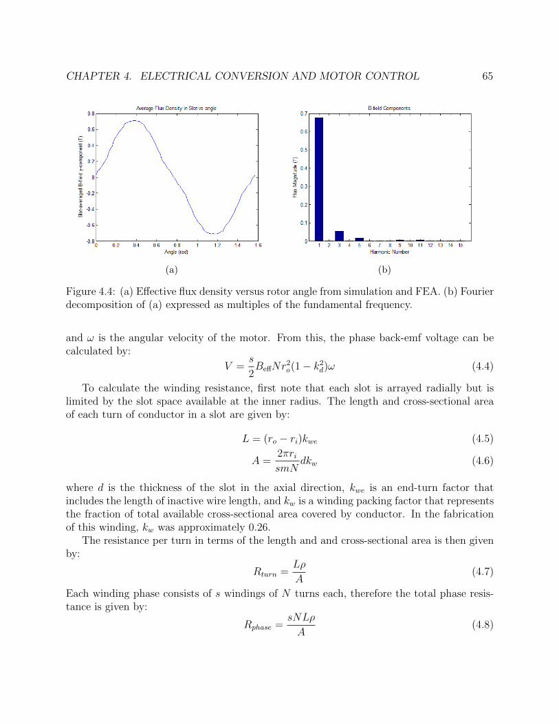
CHAPTER 4. ELECTRICAL CONVERSION AND MOTOR CONTROL 65
(a) (b)
Figure 4.4: (a) Effective flux density versus rotor angle from simulation and FEA. (b) Fourierdecomposition of (a) expressed as multiples of the fundamental frequency.
and ω is the angular velocity of the motor. From this, the phase back-emf voltage can becalculated by:
V =s
2BeffNr
2o(1− k2
d)ω (4.4)
To calculate the winding resistance, first note that each slot is arrayed radially but islimited by the slot space available at the inner radius. The length and cross-sectional areaof each turn of conductor in a slot are given by:
L = (ro − ri)kwe (4.5)
A =2πrismN
dkw (4.6)
where d is the thickness of the slot in the axial direction, kwe is an end-turn factor thatincludes the length of inactive wire length, and kw is a winding packing factor that representsthe fraction of total available cross-sectional area covered by conductor. In the fabricationof this winding, kw was approximately 0.26.
The resistance per turn in terms of the length and and cross-sectional area is then givenby:
Rturn =Lρ
A(4.7)
Each winding phase consists of s windings of N turns each, therefore the total phase resis-tance is given by:
Rphase =sNLρ
A(4.8)

CHAPTER 4. ELECTRICAL CONVERSION AND MOTOR CONTROL 66
The end turns are arrayed azimuthally at both the inner and outer radius, therefore theadditional end-turn factor kwe is given by:
kwe =(1− kd) + 4π
sm(1 + kd)
1− kd= 1 +
4π
sm
(1 + kd)
(1− kd)(4.9)
Plugging this equation and the equations for length and cross-sectional area into the phaseresistance equation, and making the substitution kd = ri
ro, the expanded equation for phase
resistance is given by:
Rphase =s2mN2ρ
2πdkw
(1− kdkd
)(1 +
4π
sm
(1 + kd)
(1− kd)
)(4.10)
From this and the EMF per phase, the V 2
Rmetric is given by:
V 2
R=
s2
4B2
effN2r4o(1− k2
d)2ω2
s2mN2ρ2πdkw
(1−kdkd
)(1 + π
sm(1+kd)(1−kd)
) (4.11)
=πB2
effN2r4oω
2dkw2mρ
(1− k2d)
2(1−kdkd
)(1 + π
sm(1+kd)(1−kd)
) (4.12)
=πB2
effN2r4oω
2dkw2mρ
kar (4.13)
where kar is defined as the aspect ratio factor kar =(1−k2d)2(
1−kdkd
)(1+ π
sm
(1+kd)
(1−kd)
) . kar is independent
of most machine parameters, such as the B-field, motor speed (ω), overall radius (ro), andslot thickness (d); the only dependent parameters are the slots per phase, s and the numberof phases, m. Therefore, maximizing kar offers general insight into the optimal geometry ofthe machine.
For the axial flux machine designed for this Stirling engine, there are three phases andeight poles, therefore s = 8 and m = 3. Given these parameters, the aspect ratio factorkar is maximized at kd = 0.51 - in other words, when the inner radius of the magnet andwinding space is half of the outer radius. The value of this aspect ratio factor over the rangeof aspect ratios is shown in Figure 4.5, showing the maximal value of kar can be seen tooccur at kd = 0.51. If the minimization of magnet volume is desired, then an additionalmagnet volume factor can be included, which further drives kar higher to approximately0.67, as shown in Figure 4.6. These conclusions agree with similar analysis in [19].
Alternator Losses
There are three main sources of loss in this alternator design: resistive winding losses, eddycurrent losses, and windage frictional losses. The resistive winding losses are simply given

CHAPTER 4. ELECTRICAL CONVERSION AND MOTOR CONTROL 67
Figure 4.5: The value of kar over varying aspect ratios reaches a maximum at approximatelykd = 0.51.
by:
PΩ =1
2I2Rw (4.14)
where I is the current in the windings and Rw is the resistance of the windings. Thisis calculated for each phase and summed together. The design and optimization aroundthe V 2/R metric already serves to minimize the quantity of these losses. A first-orderestimate of the resistance of the windings was 112 mΩ. This, however, only accounts for thecore resistance component of the windings; it did not account for contact resistances andadditional wire length for interconnecting windings and
Eddy current losses occur due to small circulating currents in conductors caused by chang-ing magnetic fields. Since there is no stator back-iron, the only conductor that contributeseddy losses are the copper wires. The wires were chosen as fine-strand litz wire bundles, withindividual strands of 30 gauge wire, in order to manage eddy current losses. The equation

CHAPTER 4. ELECTRICAL CONVERSION AND MOTOR CONTROL 68
Figure 4.6: The aspect ratio factor normalized by magnet volume.
for eddy current loss is given by [28]:
Peddy =1
16σω2d2Vcond
∞∑n=1
n2(B2myn +B2
mzn
)(4.15)
where σ is the conductivity of the material, ω is the angular frequency of alternating mag-netic fields (which is not the same as the engine cycle frequency), d is the diameter of theconductors in the gap, Vcond is the volume of conductors, n is the harmonic order number,and Bmyn and Bmzn are the harmonic components of the magnetic flux density that aretransverse to the conductor. The flux density component that is parallel to the conductor isnegligible due to the small cross-section of the wire. With a good magnetic design in whichflux at the windings is almost entirely oriented in the axial direction, as is the case with thismachine, the Bmzn component is also negligible and can be ignored. The summation in theequation is over the harmonic orders of the flux density, with higher order harmonics scaling

CHAPTER 4. ELECTRICAL CONVERSION AND MOTOR CONTROL 69
up quadratically with the order. The eddy current losses for this machine are calculated tobe below 2 W.
Windage losses are frictional losses from moving air, caused by the relative motion of therotor.
Pwindage =πω2µ(r4
o − r4i )
2g(4.16)
where ω is the mechanical angular frequency of the rotor, µ is the dynamic viscosity of theair between the rotor and stator, and g is the air gap between the rotor and stator. For theelectric machine at hand, the windage losses were conservatively estimated to be less than0.08 W, and therefore negligible. Magnetic core losses are also a signficiant component ofloss in typically motor-alternators, but since the stator is coreless in this design, this sourceof loss is negligible.
4.2 Drive Controls
The Stirling engine required the development of custom motor drive controls to overcomethe challenges associated with startup. A commercially-available motor drive was initiallyused, but was unable to start up the Stirling engine due to a high torque requirement at lowspeed. This is due to the significant force required to initially compress the gas volume ofthe engine in order to complete the first half-cycle of the engine. This compression requiresa large activation energy to be overcome at startup. The controls developed to overcomethis challenge and to run the Stirling engine during normal operation are described in thissection.
While this compression energy is a significant challenge for startup, it is mitigated duringoperation by the design of the power piston as a resonant system. The gas volumes andpower piston mass were specifically chosen to form a resonant mass-spring system at thenominal operating frequency, therefore minimal drive is required to sustain motion. Inaddition, when a temperature differential is present and the displacer is activated, the Stirlingcycle provides a thermodynamic driving force that biases the engine toward the forward(generation) direction. This effect also serves to reduce drive requirements during nominaloperation, but not during startup. Therefore, the most challenging part of the motor driveis startup. To address the challenge of startup, a custom mechanically-resonant PWM drivewas developed to overcome this initial barrier.
It should be noted that the engine at rest had the power piston in the fully expandedstate. This added to the startup challenges by requiring even greater initial compressionto begin engine motion. An alternate configuration could have allowed the power pistonto begin in a neutral compression position when at-rest, and would have eased the startupcompression required. Nonetheless, the development of the custom resonant startup drive isrelevant even in that case, as the compression forces required are still high.
The motor controls were implemented on a National Instruments sbRIO-9632, a boardthat combines an FPGA with a real-time operating system on a microcontroller. The control

CHAPTER 4. ELECTRICAL CONVERSION AND MOTOR CONTROL 70
algorithms were developed and programmed through LabView. The core of the control coderan on the FPGA, while the real-time OS was used for management, configuration, HMI,and data logging. The control algorithm used measurements of three-phase voltages andcurrents at the motor terminals in a sensorless scheme and generated PWM signals to run acustom lab inverter. An observer was used to estimate the phase angle of the motor basedon three-phase voltage measurements.
The controls had three stages of operation. The initial stage was simply an open-loopimpulse to generate enough motion for the observer to lock on. The second stage is a resonantstartup mode designed to overcome the compression work required to begin spinning. Ratherthan attempting to produce high torque at low speed to overcome compression forces, thedrive added energy at the resonance of the piston motion. This leveraged the behavior of thepiston and gas spring as a mass-spring system to gradually impart energy into the systemover the course of multiple cycles. By adding energy at the resonance of the system, thetotal activation energy required to begin normal operation could be added incrementally atlower torque over a longer period of time. The energy of the system is increased over thecourse of multiple cycles, gradually increasing the swing amplitude, until there is sufficientenergy to overcome the compression barrier. The final stage of operation is normal engineoperation, and takes place after the piston has built up enough momentum for sustainedrotation. These controls will be discussed in the following subsections.
System Equations
First, the Stirling engine, motor/alternator, and electrical interface will be described by aset of state equations in a dynamical state-space system model. These three subsystems areeach described by differential equations, which when combined characterize the behavior ofthe overall system. The state variables in these system equations are the angular positionof the engine, θ, the angular velocity of the engine, ω, and the three-phase current in theelectrical circuit, i.
The Stirling engine mechanical system is modeled as a rotating mass with rotationalinertia and frictional damping, along with PV forces from the Stirling cycle and gas spring.The motor contributes torque to the system, leading to the following engine equation:
Jd
dtω + bω + kc sin θ = τm + τS(θ) (4.17)
where J is the rotational inertia of the engine, θ is the engine angular position, with angle 0designated as the central position of the power piston, b represents frictional damping forces,kc is the effective gas spring constant, τm is the applied motor torque, and τS(theta) is drivefrom the Stirling cycle conversion between thermal and mechanical energy, and is negativefor the engine operating in motor mode and positive for generation mode.
The gas spring and Stirling drive terms, kc sin θ and τS(θ), comprise the combined PVforces of the working fluid in the Stirling engine. The PV forcing of the Stirling cycleis disaggregated in this manner to represent real and reactive components of the cycle, in

CHAPTER 4. ELECTRICAL CONVERSION AND MOTOR CONTROL 71
much the same way that AC power can be real and reactive. The gas spring term contributesforces throughout the cycle, but imparts zero net energy over a cycle, aside from losses, andis therefore analogous to reactive AC power. This term represents the component of gasforces that would still be present even in the absence of a temperature differential, andtherefore without any thermal energy conversion. The Stirling cycle conversion drive term isthe core energy conversion process of the Stirling engine, and is manifested as additional PVforces (on top of gas spring forces) from thermal energy transfer into or out of the workingfluid. This is analogous to real power in an AC system, since it represents the power that isconverted and delivered during the net Stirling cycle.
The electrical circuit includes the three-phase inverter and the motor/alternator, whichis represented by a back-emf and a series resistance and inductance. The equation for theelectrical circuit is:
Ld
dti+Ri = Vi − Ve (4.18)
where L is the per-phase inductance between the motor and inverter, R is the per-phaseresistance, Vi is the inverter voltage, i is the current, and Ve is the back-emf. Since themotor/alternator is a three-phase machine, the voltages and currents in this equation arethree phase vectors, representing three circuits, but written here as one for simplicity.
The mechanical and electrical state equations are coupled together through the equationsfor the motor/alternator, which is represented by a motor back-emf and torque with thefollowing equations:
τm = kti (4.19)
Ve = keω (4.20)
(4.21)
where ke is the back-emf constant, and kt is the torque constant. Note that the back-emfand torque constants are numerically equal when expressed in SI units.
Combining these equations into a state space model gives the following:
d
dtθ = ω (4.22)
d
dtω =
−bJω +
kc sin θ
J− kt
Ji +
τS(θ)
J(4.23)
d
dti =−keLω +
−RLi +
1
LVi (4.24)
d
dtθ = ω (4.25)
(4.26)
Or expressed in matrix notation:

CHAPTER 4. ELECTRICAL CONVERSION AND MOTOR CONTROL 72
d
dt
θωi
=
0 1 0
0 −bJ
ktJ
0 −keL
−RL
θωi
+
0
01L
(4.27)
In this model, the motor is modeled as a combination of a back-emf component, a resis-tive component, and an inductive component. The back-emf component represents the elec-tromotive force of the motor/alternator and increases proportinally with engine frequency,multiplied by the number of pole pairs in the motor/alternator. The winding inductance wasmeasured to be (171 µH) and the winding resistance was measured to be 240 mΩ. Withinthe operating range of the Stirling engine, from low frequency startup to a peak electricalfrequency of 80 Hz, the impedance of the motor windings is predominantly resistive. Thisdiffers from typical motors, which tend to be dominated by winding inductance, and is aresult of the coreless design of the motor windings. These measured impedances were mod-eled in the control loop parametrically, and used to calculate a winding voltage drop that isthen subtracted to estimate the back-emf rotor voltage Vr. This rotor voltage was used inthe calculation of control signals.
Two-Phase Representation
In a three-phase system, there are two degrees of freedom for AC voltages and currentsaround a DC common mode, and therefore three-phase information can be fully representedby two AC values and an offset. These are obtained by a transformation from three-phasespace to a two-phase vector, called the Clarke Transformation. This helps simplify controlalgorithms, and is commonly used in motor control algorithms. The two-phase coordinatesystem generated by the Clarke Transformation is by convention labeled αβγ coordinates[6]. The αβγ representation combines a two-dimensional vector represented by α and βcomponents and an common-mode offset represented by γ. The γ component is nominallyzero in a balanced three-phase system. As long as voltages are referenced to the three-phaseneutral, and there are no alternate paths for currents to flow, then three-phase voltagesand currents sum to zero and the γ component is not needed for controls. The Clarketransformation is given by the following equation:
Xα
Xβ
Xγ
=2
3
1 −1
2−1
2
0√
32−√
32
12
12
12
Xa
Xb
Xc
(4.28)
where X is the type of quantity being transformed, namely voltage V or current I, andthe a,b,c subscripts refer to three-phase quantities and α,β,γ subscripts refer to transformedquantities. As mentioned above, for balanced three phase systems, the γ component iszero and the transformed coordinates are effectively two-dimensional. The equation can be

CHAPTER 4. ELECTRICAL CONVERSION AND MOTOR CONTROL 73
rewritten in terms of line-to-line quantities, since the measured voltages were line-to-line.Therefore, the transformation equations for voltage and current are:Vα
Vβ
=
23−1
3
0 1√3
VacVbc
(4.29)
IαIβ
=
1 0
1√3
2√3
IaIb
(4.30)
The inverse transformation is given by:
Xa
Xb
Xc
=
1 0
−12
√3
2
12−√
32
Xα
Xβ
(4.31)
The αβγ space and the Clark Transformation are conceptually similar to a Direct-Quadrature (DQ) coordinate system, with the αβγ transformation differing only in thatthe reference frame does not rotate along with the rotor angle. This was chosen over theDQ transformation because it reduces the complexity of calculatons required on the FPGA.Following discussions of currents and voltages will use the αβ vector space representationfor the purposes of the control loop.
Sensing and Observer
As shown above, three phase voltages and currents can each be determined with two mea-surements given a balanced three-phase system. During experiments, differential voltagesensors were used to measure the line-to-line voltages Va − Vc and Vb − Vc, and clamp-oncurrent sensors were used to measure Ia and Ib. These sensors were connected to Analog-to-Digital converters on the National Instruments control board, and in software were convertedinto αβ quantities.
The αβ voltage measurements are used to estimate the angular position and speed of theengine, in lieu of Hall sensors or motor shaft encoders to directly measure motor position.This scheme is called Sensorless Motor Control, eponymously referring to the lack of directsensors of motor position. Instead, an observer is implemented in software to estimate themotor position using measurements of voltage. The observer represents the electrical angleof the motor in cartesian coordinates, as a vector on the unit circle, and updates its positionbased on new measurements of the voltage. Control commands are derived from the observerin order to generate voltages related to the physical state of the motor, within a reasonableerror margin.

CHAPTER 4. ELECTRICAL CONVERSION AND MOTOR CONTROL 74
The observer can be described as a set of states and update equations. The states arethe cartesian coordinates and the angular velocity. The update equations are described bythe following equations. First, the voltage measurement is used to generate an error in themeasured angle from the observer angle at each timestep, which is calculated by the followingequation:
δθ =~Vr‖Vr‖
· ~θt (4.32)
where θt is the unit tangent vector at the observer position. δθ is the component of the newvoltage position in the direction tangent to the observer position, which is a good approx-imation for the change in angle for small deviations. This is a computationally expensivecalculation, primarily due to the division by the magnitude of the measured voltage. Anapproximation to the magnitude was made using:
‖V ‖ ≈ max(|Vx|, |Vy|) +1
4min(|Vx|, |Vy|) (4.33)
This drastically reduces the norm calculation overhead, while only incurring a 5% RMS errorover the angular domain [0, 2π). This is also equivalent to 3
4‖V ‖∞+ 1
4‖V ‖1. The level-set of
this norm is shown in Figure 4.7The observer then updates its internal state based on this angle error. A rotation update
is calculated based on both a predictive component incorporating the angular velocity andthe angle error, and the angular velocity is updated based on the angle error. Both updatesare modulated by scalar gain constants α1, α2, chosen empirically to give a sufficienctly fastresponse.
∆θ = ωk + α1δθ (4.34)
ωk+1 = ωk + α2δθ (4.35)
where ∆θ is the rotation update to be used in the next equation, ωk is the prior angularvelocity, ωk+1 is the next angular velocity, δθ is the angle error calculated previously inEquation 4.32, and α1 and α2 are the observer gains.
The rotation update from Equation 4.34 is used to update the observer vector via forwardintegration. A basic method is to use simple Euler integration, as shown in Equation 4.36.
xk+1 = xk + ∆θyk
yk+1 = yk −∆θxk (4.36)
However, Euler integration leads to accumulating unbounded error. The Euler methodis a poor choice for forward integration in all but the simplest cases, requiring very smallstep sizes to reduce error. More complicated algorithms are typically used that bound andreduce the integration error drastically, such as Runge-Kutta integration, but at the cost ofmore calculation overhead. However, since the angular position observer is constrained to a

CHAPTER 4. ELECTRICAL CONVERSION AND MOTOR CONTROL 75
Figure 4.7: The level-set of the custom norm (in blue) compared to a Euclidean L2 norm(in red).
circle, a simpler method can be used with almost no impact on computational overhead. TheGauss-Seidel method of integration (also know as Euler-Cromer), shown in Equation 4.37,eliminates the growth of integration error [10]. This is the method that is used to updatethe observer angular position.
xk+1 = xk + ∆θyk
yk+1 = yk −∆θxk+1 (4.37)
With the observer providing an estimate of the motor/alternator position, the controlloop can generate a command that drives the engine as desired.

CHAPTER 4. ELECTRICAL CONVERSION AND MOTOR CONTROL 76
Controller
The controller is responsible for generating a PWM command to the inverter in order toproduce the desired behavior of the engine. It uses the speed estimate from the observer,compared with the desired speed setpoint, to generate a current magnitude command, whichis used to generate a voltage command to the inverter. Details of the control algorithm areexplained next.
First, the speed control block, shown in Figure 4.8, calculates the error in speed betweenthe observer estimate and the speed setpoint. This error is actually calculated from thedifference between the squares of the angular velocities, rather than simple linear subtraction.This was chosen for two reasons: first, it simplifies the controls to be independent of thesigns of the observer speed estimate and speed setpoint; second, it matches the physicsdimensionally, where rotational energy is proportional to ω2. It is desirable to control aquantity that is analogous to energy as the resonant control scheme is intended as a controlon the energy of the system. The current reference is generated from the speed error bymultiplying by a feedback gain, and then scaled from the motor voltage vector in order tocommand a current in phase with the motor voltage to command unity power factor. Theequation for the control is then given by:
Iref = αspeed(ω2set − ω2
obs)Vr (4.38)
where Iref is the reference current command calculated from this block, αspeed is the feed-back gain, ωset is the speed setpoint, ωobs is the observer speed estimate, and Vr is the motorvoltage. In order to finish the resonant startup mode rotating in the same direction determin-istically, the reference current was modulated assymetrically to drive harder in one directionthan the other during the startup portion of the control. This ensures that the engine alwaysrotates in the desired direction. This is important, as the direction of rotation dictates thedirection of the thermodynamic cycle; i.e. whether the engine operates in generation modeor heat pump mode. The output of this block is the current reference used in the next step.
Figure 4.8: Schematic for generating a reference scaling factor based on observer velocityand setpoint.

CHAPTER 4. ELECTRICAL CONVERSION AND MOTOR CONTROL 77
The reference current Iref is compared to the measured current I and fed into an inte-grator to obtain the voltage control signal to drive the inverter gates with PWM. This canbe expressed as:
Vcontrol = αint
∫(Iref − Imeas) (4.39)
where Vcontrol is the voltage command output, αint is the integrator gain, Iref is the referencecurrent generated in the previous step, and Imeas is the measured current. The voltagecommand is transformed using the inverse αβ transformation to three-phase voltages andthen converted to PWM gate signals to drive the inverter.
A block diagram of the overall control scheme is shown in Figure 4.9, and a full schematicof the control algorithm is shown in Figure 4.10. The control algorithm updated at a fre-quency of 15 kHz, the same frequency as the PWM algorithm, and synchronized to update onthe FPGA at the peak values of the PWM triangle modulator waveform, thereby minimizingthe possibility of glitches or additional switching in the middle of a PWM period. The valueof the important control constants were first chosen to provide sufficient bandwidth withoutcreating instability, then refined empirically to optimize behavior based on observer fidelity,low current startup, and well-behaved control while running.
Figure 4.9: Block diagram of the overall control scheme.
This control scheme successfully allowed for a softer resonant startup by injecting energyin phase with the natural resonant motion of the engine during startup. The piston wouldundergo startup by swinging in one direction, then the other, with the controller injecting

CHAPTER 4. ELECTRICAL CONVERSION AND MOTOR CONTROL 78
energy throughout the process. Once enough kinetic energy was imparted to overcome thecompression activation energy, the engine successfully rotated and engaged in normal op-eration. This same control scheme also worked during normal operation, with the changethat the drive command was no longer assymmetrically modulated as was necessary duringstartup to ensure rotation in the desired direction. The implementation of the this resonantcontrol scheme significantly reduced the startup currents. While previous algorithms com-manded upwards of 80 A, resonant startup using this control scheme reduced mean currentsto under 10 A, with brief peaks at 20 A.
The software layer above the control algorithm consisted of reading measured and gener-ated data through the FPGA FIFO, displaying and graphing the control front panel interface,and relaying user setpoints and configurations down to the FPGA. This ran on the real-timeOS portion of the board in order to save FPGA space, and ran at a signficantly slower speed,at about 10 Hz. An additional service ran on the host computer, which simply logged datacontinuously to the disk.

CHAPTER 4. ELECTRICAL CONVERSION AND MOTOR CONTROL 79
Figure 4.10: Schematic of the overall control scheme.

80
Chapter 5
Experimental Results
This chapter will discuss the results of various experiments, how the data compares to pre-dictions, and the implications for the Stirling engine system as designed. The experimentalstage focused on assessing the performance of heat exchangers and thermal transfer, on quan-tifying losses in the system, and on quantifying the Stirling cycle behavior of the engine.
Even though this engine was designed with a specific application in mind, the primarypurpose of experimentation was to confirm that the design process was accurate and robust,rather than demonstrating a commercially ready engine. A commercially ready prototypehas different requirements from a research prototype and would likely require significantchanges or additions, in particular to the pressure containment structure, to the fabricationand assembly process of components, and the integration of a solar-heated fluid loop. Thesame design procedure would be fully appropriate for such a prototype, however, and remainsthe most important contribution.
The process of testing and experimentation happened over several stages, which will bedescribed in the followings sections. The first stage was assembly and testing of componentsof the engine to verify correct high-level operation. This required the refinement of severalcomponents in order to produce the desired behavior. The next stage was to conduct isolatedtests on particular components to confirm particular design predictions. Finally, experimentswere conducted with the fully assembled engine of thermal behavior, Stirling cycle heat pumpoperation, and engine operation.
5.1 Assembly and Verification
After the core engine components were fabricated, assembly and verification were performedto confirm proper operation at a high level. As part of this stage, the assembly procedurefor the engine was tested and refined. The assembly procedure was greatly simplified withslight modification or a few components. In brief, the crankshaft and piston componentsare first assembled together around the cold-side steel plate, which serves as the structuralfoundation for the rest of the engine. Then heat exchanger and regenerator components are

CHAPTER 5. EXPERIMENTAL RESULTS 81
assembled, and the engine is then enclosed by its containment shell and insulated externally.The alternator is then assembled; first the rotor magnet discs are mated together on either-side of the stator, then the rotor is attached to the crankshaft and the stator attached to thecold-side steel plate. Finally, the engine is lifted into the pressure vessel. A series of picturesshowing stages of the engine assembly process is given in Figure 5.1.
During this stage, two significant problems were identified. One was intermittent scrapingof the displacer piston against its cylinder. This was caused by a combination of higher thanspecified angular play in the linear sliding bearing of the displacer piston rod, and out-of-speccircularity and flatness in the displacer ring and plates. The latter issue required additionalmachining to bring the parts into spec. However, the former issue required rethinking ofthe bearing mechanism for the displacer rod. As mentioned in Chapter 3, a double-bearinghousing, incorporating two of the linear sliding bearings along the same axis, was designedto structurally reduce angular play in the displacer piston rod and enforce linear motion. Aschematic of the double-bearing housing was shown in Figure 3.15a. The second significantproblem was runout in the crankshaft end. This caused large out-of-plane deviation in thespinning magnet disc, causing interference with the stator. This was fixed with a combinationof re-machining and by mounting the stator to adjustment bolts to tune its position.
There is a notable difference between the prototype as assembled and a hypotheticalcommercial system. Due to the constraints of lab experimentation, the hot side externalfluid loop could not be implemented to provide the full quantity of heat, which would haverequired a significant boiler. Instead, electric heating was installed on the hot side as a proxyfor whatever heat source would be present in an actual application, as shown in Figure 5.2.This greatly simplified the construction of the experimental apparatus, as well as allowedfor much more accurate measurements of input thermal power. The characterization ofthe engine thermal performance is still complete, except for the hot-side external fluid-to-metal component. However, this component of hardware is identical to the cold-side, whosecharacterization serves as a reasonable proxy. Identical equations are used in the design ofboth cold-side and hot-side versions, so verication on the cold-side serves to validate themodel nonetheless.
5.2 Heat Exchanger Test
The heat exchangers represent one of the most important components in the engine. As such,a number of tests were conducted to verify their performance. The important properties totest were the external fluid to body heat transfer, heat transfer through the body, and bodyto working fluid heat transfer.
The first type of experiment tested the heat transfer through the body and throughthe mesh. Heating elements were applied to the external face of the heat exchanger, withan applied heating power of 500 W, and thermocouples were placed throughout the heatexchanger structure. Temperature drops were measured throughout the heating transient.This test was repeated twice. The results of the test are compiled in Table 5.1. This table

CHAPTER 5. EXPERIMENTAL RESULTS 82
(a) (b)
(c) (d)
Figure 5.1: Pictures of the engine assembly procedure in several stages. (a) shows the engineassembled with crankshaft and pistons. (b) shows the assembly of the magnet rotor discsaround the stator using a drill press. (c) shows the alternator assembled on the end of thecrankshaft. (d) shows the engine fully assembled.

CHAPTER 5. EXPERIMENTAL RESULTS 83
Figure 5.2: The electric heater assembly is shown here, bolted against the external side ofthe hot-side heat exchanger.
Component Average Temperature Drop
External face to internal channel ridge 0.12 K
Mesh contact ridge to mesh interior 0.10 K
Table 5.1: Heat exchanger body and mesh conduction temperature drops.
shows two temperature drops: first, the temperature drops from the surface in contact withthe external fluid to the ridge on the internal side of the heat exchanger that contacts themesh; second, the temperature drop from where the mesh contacts the heat exchanger bodyto the center of working fluid flux region. This test confirmed that these temperature drops,which were predicted to be small but difficult to precisely calculate due to the high variancebased on empirical conditions, were in fact appropriately small.
A second thermal experiment tested the full path of heat flux with the engine entirelyassembled. During this test, electric heating was applied at the hot-side external face,while the cooling fluid loop was running at the cold-side. The engine was not in motionduring this test. The thermal heating transient was recorded, along with the equilibriumstabiliation temperature profile through the engine, and the cooldown transient was alsorecorded. This allows characterization of thermal properties in the context of the assembledengine. In particular, this test quantifies static leakage heat fluxes in the engine, includingheat conduction losses, heat transfer to the external fluid, and losses to the pressure vessel

CHAPTER 5. EXPERIMENTAL RESULTS 84
Component Heat Flux Temperature Drop
Total Input Power 2183 W
Cold-Side External Fluid 1873 W 0.30 C
Losses to Vessel Ambient 310 W 144 C
Engine Internal Cylinder 223 W 143.1 C
Table 5.2: Heat exchanger temperature drops.
environment. Results from this experiment at thermal equilibrium are compiled in Table 5.2.The total input power was measured by calculating the electrical input power to the
heaters. The heat flux into the cold-side external fluid was obtained by measuring thetemperature drop between the inlet and outlet, and multiplying by the heat capacity flowrate of the fluid. The losses to ambient were calculated as the difference between these twoheat fluxes. The engine internal cylinder temperature drop was calculated as the differencein measured temperature between thermocouples contacting the internal cylinder at the hotside and cold side, and the heat flux was calculated from the temperature drop by modelingthe internal cylinder as a thermal resistance due to conduction. This heat flux is included inthe heat flux to the cold-side external fluid, as the heat loss is still delivered to the cold-sidefluid. This test confirms that the engine behaves as designed with respect to static heatfluxes, most importantly in two ways. First, that the cold-side fluid heat exchanger properlycools the engine, as evidenced by a 2.3 C temperature drop from the heat exchanger metal tothe fluid, compared to a predicted 2.6 C temperature drop. Second, that conduction lossesthrough the engine are isolated to the predicted paths such as the internal cylinder, and thatthere are no other unexpected non-negligible thermal leakage paths. This is evidenced bythe internal cylinder maintaining nearly the full temperature differential (174.7 C to 32.3 C)under equilibrium.
A third thermal experiment was performed in conjunction with the heat pump and gen-eration tests, to be fully described later. This test differs from the prior tests primarilyin that it is testing for oscillatory thermal behavior rather than static thermal behavior.This allows verification of the mesh-to-air heat transfer characteristic, which is the mostsignificant component of the heat exchanger’s overall performance. This test incorporateda heating transient, equilibrium measurements, and a cooldown transient. The most directmeasurement of the mesh-to-air heat transfer performance is the equilibrium measurement.In this measurement, the temperature drop from the mesh to air was measured to be 1.5 C,while the design value under these operating conditions was 3.1 C. The improvement of themeasured value over the design value is most likely simply due to the fact that the mostconservative empirical model of mesh-to-air heat transfer was chosen as the basis for design.The experimentally measured values and design values are listed in Table 5.3.
By combining the results of these three tests, an overall characterization of the heat

CHAPTER 5. EXPERIMENTAL RESULTS 85
Mesh-to-Air Property Measurement Design
Hot-side Temperature Drop 1.7 C 3.1 C
Cold-side Temperature Drop 1.5 C 2.7 C
Table 5.3: Heat exchanger temperature drops after reaching equilibrium during heat pumptest.
Heat Exchanger Property Measurement Design
External fluid to body resistance 1.66× 10⁻⁴ C/W 1.75× 10⁻⁴ C/W
Body path 6.1× 10⁻⁵ 5.51× 10⁻⁵ C/W
Body to mesh (longest path) 4.2× 10⁻⁵ C/W 3.97× 10⁻⁵ C/W
Mesh to working fluid (Hot side) 2.70× 10⁻⁴ C/W 2.70× 10⁻⁴ C/W
Mesh to working fluid (Cold side) 1.5× 10⁻⁴ C/W 2.33× 10⁻⁴ C/W
Table 5.4: Heat exchanger temperature drops after reaching equilibrium during heat pumptest.
transfer properties of the heat exchangers can be made. A table listing the measured valuesversus the design values is given in Table 5.4.
5.3 Alternator Performance
The alternator was also tested and compared to predictions from the design process. Themost important performance characteristics to be determined are the efficiency of the alter-nator, and the harmonic content of its associated waveform. The efficiency of the alternatoris affected primarily by the electrical resistance of the windings. As previously discussed inChapter 4, back-iron losses are neglibile, and eddy losses and windage are orders of magni-tude less than resistive loss and accordingly difficult to measure. The design resistance ofthe windings was 249 mΩ per phase, while the measured resistance was 240 mΩ per phase.
The EMF waveform of the alternator was predicted in the design phase with flux datafrom FEA combined with a winding model and simulation. This waveform can be comparedto the actual measured waveform in the time domain and frequency domain.
5.4 Loss Experiments
Measuring the losses or deviations from ideality in the engine is a highly important partof engine characterization. There are a variety of different loss mechanism, detailed in

CHAPTER 5. EXPERIMENTAL RESULTS 86
Figure 5.3: Plots of the motor back EMF as predicted during the design phase versusmeasured during tests.
Chapter 3, each of which require different experiments or methods of discernment. Sincemany of these losses are small, measurement in these cases can only accurately verify thatthey fall within the bounds of expectation, which is in itself a valuable exercise for thepurposes of evaluating the Stirling engine design process.
A number of the losses only occur in the engine when it is actually operating. Theseinclude flow frictional losses in the mesh, air-channel frictional losses, displacer and powerpiston running losses. To separate and independently characterize these operating losses, aseries of experiments was performed with the engine driven by the alternator, with compo-nents installed or removed in successive tests in order to isolate their effects. The change inpower required to drive the engine therefore indicates the loss value of the change in installedcomponentry. The baseline was established by measuring driving power with only the al-ternator and crankshaft, without any additional components. This allows measurement of abaseline level of operating losses in the engine - that of the crankshaft bearings and motion.Subsequent tests measured various combination of installed components, which are detailedin Figure 5.4.
These tests were all performed at full pressurization at 30 bar and full frequency at 20 Hz,the only exception was the Compression Test which was performed at 16.2 bar and full

CHAPTER 5. EXPERIMENTAL RESULTS 87
Baseline Test - Crankshaft only - Measures bearing losses and crankshaft drag loss
Displacer Test - Crankshaft and displacer piston - Measures displacer flow friction losscompared to baseline
Heat Exchanger Test - Crankshaft, displacer, and 1x heat exchanger - Measures singleheat exchanger flow friction loss compared to Displacer Test
Regenerator Test - Crankshaft, displacer, 1x heat exchanger, and regenerator, partialenclosure - Measures regenerator flow friction loss compared to Heat Exchanger Test
Power Piston Test - Crankshaft and power piston - Measures Power Piston flow frictionand bearing loss compared to Baseline Test
Full Heat Exchanger Test - Crankshaft, displacer, both heat exchangers, regenerator,full enclosure - Measures and confirms heat exchanger loss compared to RegeneratorTest
Compression Test - Crankshaft, power piston, both heat exchangers, regenerator, fullenclosure - Measures compression loss compared to Full Heat Exchanger Test.
Figure 5.4: Descriptions of the spinning loss tests, the installed components in each test,and the marginal loss component gleaned from each test.
Loss Component Measured Loss Predicted Loss
Bearing and Crankshaft Loss 3.9 W <10 W
Displacer Flow Friction Loss 12.3 W <20 W
Heat Exchanger Flow Friction Loss 61 W 24.7 W
Regenerator Flow Friction Loss 102.5 W 115 W
Power Piston Flow Friction Loss 22.4 W <50 W
Compression Loss 72 W 54.7 W
Table 5.5: Measured and predicted spinning losses for various loss components, with theexperiments described in Figure 5.4
frequency, and compared to repeated versions of the other tests under the same conditionsin order to isolate the compression loss. By subtracting the losses from these tests andattritbuting the difference to the effect of specific components, individual component lossescan be disaggregated. These disaggregated loss measurements from these tests are listed inTable 5.5.
A few important comments should be made regarding the losses presented in Table 5.5.

CHAPTER 5. EXPERIMENTAL RESULTS 88
First, certain losses could not be determined precisely during the design process. These arechiefly due to the difficulty in calculating bearing losses, which can vary based on minutedetails or features in the fabrication or assembly process. Instead, these bearing losses hadupper bounds that were estimated in accordance with conservative empirical formula. Theresults show that measured bearing losses were indeed within the bounds given.
Second, most measured losses matched their design values. This validates much of thedesign effort to quantify and account for losses. However, the mesh flow friction loss standsout as being signficantly greater in measurement than in design. This discrepancy is notentirely unforeseen. During design, the calculation of this loss is made assuming uniform flowthroughout the mesh. However, this is not entirely accurate, as higher flow occurs closer tothe displacer piston, both in the air channel and through the mesh. These areas of higher flowgenerate greater losses than the reduction in losses elsewhere due to lower flow rate, due tothe quadratic scaling of flow loss with velocity. The total effect is to increase the losses fromthis component. This effect cannot be easily accounted for, however, without incorporatingfluid dynamics modeling into the loss calculation. A second unaccounted effect is due to thefact that the design analysis for mesh flow friction loss assumes uniformity in the structureof the mesh. In the actual assembly of the mesh in the heat exchanger, non-uniformitycan occur due to differing fiber alignment between layers. This introduces additional flowfrictional loss, as the working fluid is impeded in moving through layers of fiber. For a moreaccurate design, fluid simulations could be incorporated into the design process.
The sum total of these spinning losses, however, remains close to design predictions. Thisindicates that the design process for losses at least represents a reasonable estimate of actualperformance.
5.5 Forward and Reverse Operation
The most complete experiments for verification of the design were performed by running thefully assembled engine in forward and reverse directions, which respectively correspond toheat pump and generation modes. These tests fully engage the Stirling cycle conversion ofthe engine, static losses, and spinning losses. Running in heat pump mode requires inputpower to move heat from the cold side to the hot side, while running in generation modeconverts heat moving from the hot side to the cold side into output work. The two modesare thus inverses of each other and complimentary. The experiment was designed to takeadvantage of this and exercise both modes throughout a single test. First, the engine wasdriven in heat pump mode to build up a reservoir of heat at the hot side; then it was startedin the forward direction to move the stored heat back from the hot side to the cold side.This dual-mode procedure is also how the engine could be used in a thermal-electric energystorage system.
During this phase of testing, driving the engine at full pressuriation was a significantchallenge. The current required for starting up the engine taxed the drive hardware, some-times exceeding the ratings of the IGBT modules and causing failures. After repeated stress

CHAPTER 5. EXPERIMENTAL RESULTS 89
from startup, the displacer piston began to scrape the internal cylinder, limiting the abilityto test at higher power. As a result, the heat pump and generation tests were conducted athalf pressurization and half-frequency, at 16.2 bar and 9.6 Hz. Even though this was not atthe full-rating of the engine, this still allows complete measurement and characterization ofthe engine, and the design performance was re-evaluated at exactly these conditions for anexperimental comparison.
In evaluating the full operation of the engine, one of the most useful metrics is the P-Vcurve. The P-V curve that the engine traces through represents the action of the StirlingCycle, and comparison with the simulated P-V curve is a useful qualification of the model.The area within the curve is per-cycle work developed by the Stirling Cycle, as predictedby the adiabatic simulation. The experimental P-V curve is produced from measurementsof pressure and extraction of engine volume, which is calculated by an observer looking atthe three-phase electrical vector, in conjunction with a once-around encoder to align withmechanical phase angle and synchronize on every cycle. The pressure was measured witha Honeywell A-5 Mid 100 psi -range gauge, which is a differential transducer measuringbetween the engine internal pressure and the pressure vessel ambient pressure. The enginevolumes were calculated by using the observer estimate of the electrical angle, and then usingthe once-around encoder, which was positioned to correspond to the zero-crossings in thefirst phase. This allows extraction of the mechanical angle, and therefore the engine volume,which is well-defined the by rigid pistons. Selected time-domain waveforms of the pressure,encoder, voltages and currents are displayed in Figure 5.5.
Combining the measured pressure and volume into a P-V diagram provides insight intothe thermodynamic behavior of the engine. Comparing to the simulated P-V diagram offersa high degree of validation of the model and adiabatic dynamic simulation of the engine, andalso offers insight into the performance of the engine. P-V diagrams of the engine operatingin forward (generation) mode are shown in Figure 5.7, and P-V diagrams of the engineoperating in reverse (heat pump) mode are shown in Figure 5.6. The graphs show both themeasured P-V trajectory as a scatter plot as well as the simulated P-V trajectory at theoperating conditions of the test.
As seen in Figure 5.7 and 5.6, there is agreement between experimentally derived P-V curves and the predicted curves from the Stirling engine model and simulation. Theset of P-V curves shows a variation over temperature differential that is predicted by thesimulation. At lower temperatures differentials, the P-V curve is narrower since there is lessdeveloped work in each cycle of the engine. The noise in the measured P-V curve is due toa combination of sensor noise in the pressure, voltage, and encoder sensors, numerical errorsin analog to digital conversion, and errors in the observer estimating the engine position. Atlower temperature differential, the signal-to-noise ratio is lower and the measured P-V curvematches less closely to the simulated curve.
These experiments enabled comparison of experimentally measured work with predictedwork from the design phase. The input electric power to the engine is measured at theelectric terminals of the motor/generator, as AC voltages and currents, which together givethe electric power flowing into or out of the machine, depending on direction of operation.

CHAPTER 5. EXPERIMENTAL RESULTS 90
(a) Measured Pressure Waveform (b) Measured Encoder Output (filtered)
(c) Measured Three-Phase Currents (d) Measured Voltages
Figure 5.5: Representative time-domain waveforms from measurements during engine test
Driving the engine in heat pump mode requires power to overcome losses on top of thepower required to power the Stirling cycle engine itself. In other words, the input powerrequired to drive the engine in heat pump mode is the sum of the Stirling cycle work andlosses. In generation mode, the power extracted is equal to the Stirling cycle work, minus thesame losses. Therefore, engine losses are a burden in both directions. The engine work canbe determined in either direction by disaggregating the measured losses, which have beenmeasured in separate experiments. After subtracting these losses, the measured engine workis listed in Table 5.7 and Table 5.6 over different temperature differentials.
The measured Stirling cycle power, disaggregated from losses, matches the predictionvalues from the design phase over most of the operating points tested. At lower temperaturedifferentials, the measured power values diverge more significantly from predicted values.This is possibly due to greater relative effect of measurement error on the calculated values,as the output work at these operating points has a reduced signal-to-noise ratio.

CHAPTER 5. EXPERIMENTAL RESULTS 91
(a) PV diagram with 20 C temperature differ-ential
(b) PV diagram with 30 C temperature differ-ential
(c) PV diagram with 40 C temperature differ-ential
(d) PV diagram with 50 C temperature differ-ential
Figure 5.6: P-V diagrams for heat pump mode are shown with data from measurementsplotted together with predicted curves at that operating point, over different operating pointsof temperature differential.
The measured electrical work at the motor terminals for both heat pump operation andengine operation include mechanical losses. The electrical power in these two modes can becombined for further analysis, as shown in Table 5.8. The difference between electrical powersubtracts out losses, which are roughly equal in both modes when at the same operatingpoint, giving a combined power value that is representative of the round trip power level incycling the engine as an energy storage device.
Since these tests exercise the full operation of the Stirling engine in forward engine modeand reverse heat pump mode, they provide confidence in the methodology presented inChapter 3 for analyzing, designing, and optimizing the Stirling engine. A shortcoming of

CHAPTER 5. EXPERIMENTAL RESULTS 92
(a) PV diagram with 20 C temperature differ-ential
(b) PV diagram with 30 C temperature differ-ential
(c) PV diagram with 40 C temperature differ-ential
(d) PV diagram with 50 C temperature differ-ential
Figure 5.7: P-V diagrams for engine mode are shown with data from measurements plottedtogether with predicted curves at that operating point, over different operating points oftemperature differential.
these tests is that they were not conducted at the full level of pressuriation and speedthat were presumed for the design of the engine. This would require redesign of certainmechanical components or configurations, in particular to lessen the difficulty of startup athigh pressure. However, beyond validating the design process, this prototype also providesimportant lessons for potential changes in mechanical design to address this issue, which willbe discussed in Section 6.1.

CHAPTER 5. EXPERIMENTAL RESULTS 93
PV Work in Heat Pump Mode
∆T Measured Predicted
20 C 80.3 W 120.4 W
30 C 132.2 W 187.4 W
40 C 225.1 W 252.2 W
50 C 325.1 W 317.4 W
Table 5.6: Measured Stirling cycle work during heat pump operation compared to predictedvalues from the design process.
PV Work in Engine Mode
∆T Measured Predicted
20 C 37.6 W 45.9 W
30 C 105.1 W 118.7 W
40 C 171.2 W 188.9 W
50 C 244.6 W 253.6 W
Table 5.7: Measured Stirling cycle work during engine operation compared to predictedvalues from the design process.
Engine and Heat Pump Combined Power
Engine Electrical Power Out 120.2 W
Heat Pump Electrical Power Out −449.4 W
(Engine - Heat Pump) / 2 284.8 W
Table 5.8: Combined electrical power of heat pump and engine mode at 50 C

94
Chapter 6
Conclusion
6.1 Future Work
To continue this research, there are both technical and commercial areas in which futurework would be fruitful. In the technical domain, the Stirling engine prototype built could beimproved in a number of ways. The startup process was difficult as was described previously,and could be improved simply be changing the neutral resting position of the pistons. Thedisplacer piston design presented repeated mechanical problems, and could be greatly im-proved with more mechanical engineering attention, in particular with respect to alignment,bearings, and tolerances. The experimental prototype also took liberties with the method ofpressurization, enclosing the engine in an external pressure chamber, which simplified the de-sign, but is likely cost-prohibitive. Further engineering to integrate the pressure containmentinto the engine itself would be necessary to develop a viable commercial model.
In the commercial space, further research is needed into the specific market applicationsthat would be most suited for initial deployment. While the potential addressable market forthe technology is large, much of that market is not commercially accessible until the systemis further along the cost curve. Identifying the most promising early markets would be ofkey strategic value. In addition, reducing the cost of certain components in the prototypedesign, such as the copper mesh material, would greatly improve the commercial viability ofthe system.
6.2 Final Words
The Stirling engine described in this dissertation points toward the potential for a distributedsystem that can efficiently and reliably generate renewable electricty combined with heat.The application space for Stirling systems is large, from residential generation in a moderngrid setting to microgrids in areas lacking a reliable grid. The combined benefits of electricitygeneration, energy storage, and heat energy are a attractive combination. The potential forthis technology to play a role in decarbonizing humanity’s energy portfolio is compelling.

CHAPTER 6. CONCLUSION 95
The primary goal of this dissertation is to demonstrate the potential for a Stirling enginesystem as a clean energy technology and to prove a design methodology that can be usedfor continued development of such a system. To that end, the design process was provenout in experimental tests as a way to design and optimize a Stirling engine system. Theprototype built and tested delivered for the purposes of experimental validation of the designprocess, and challenges and lessons from this iteration can guide a path forward for futuredevelopment.

96
Bibliography
[1] U.S. Energy Information Administration. How much electricity is lost in transmissionand distribution in the united states? http://www.eia.gov/tools/faqs/faq.cfm?
id=105&t=3.
[2] International Energy Agency. International energy agency.
[3] Galen L. Barbose and Naım Darghouth. Tracking the sun viii: The installed price ofresidential and non-residential photovoltaic systems in the united states, 2015.
[4] AIT/FIA Information Center. World-wide fuel list, 2012.
[5] McKinsey & Company. Mckinsey on sustainability and resource productivity, 2012.
[6] W.C. Duesterhoeft, Max W. Schulz, and Edith Clarke. Determination of instantaneouscurrents and voltages by means of alpha, beta, and zero components. American Instituteof Electrical Engineers, Transactions of the, 70(2):1248–1255, 1951.
[7] Pacific Gas & Electric. Self-generation incentive program, 2016.
[8] Sandra I. Erwin. How much does the pentagon pay for a gallon of gas? NationalDefense Magazine, April 2010.
[9] Alliance for Rural Electrification. Alliance for rural electrification.
[10] Gene H. Golub and Charles F. van Van Loan. Matrix Computations (Johns HopkinsStudies in Mathematical Sciences)(3rd Edition). The Johns Hopkins University Press,3rd edition, 10 1996.
[11] Mike M. He, Evan M. Reutzel, Xiaofan Jiang, Randy H. Katz, Seth R. Sanders, David E.Culler, and Ken Lutz. An architecture for local energy generation, distribution, andsharing. IEEE Energy2030 Conference Proceedings, Nov 17-18 2008.
[12] Caterpillar Inc. Caterpillar diesel generation sets, 2013.
[13] Frank P. Incropera. Fundamentals of Heat and Mass Transfer. John Wiley & Sons,2006.

BIBLIOGRAPHY 97
[14] Jeff St. John. The numbers behind tesla and solarcitys home energy storage play, 2013.
[15] J. Jorgenson, P. Denholm, and M. Mehos. Estimating the value of utility-scale solartechnologies in california under a 40National Renewable Energy Laboratory, May 2014.
[16] Aron Kirschner, Roger Chen, Matt Lucas, Sarah Buchwalter, and Shai Ginsburg. Dis-tributed generation from a high-efficiency, low-cost stirling engine, 2012.
[17] Lawrence Livermore National Laboratory. Estimated u.s. energy use in 2012. https:
//flowcharts.llnl.gov/.
[18] Chen Li and G.P. Peterson. The effective thermal conductivity of wire screen. Interna-tional Journal of Heat and Mass Transfer, 49(2122):4095 – 4105, 2006.
[19] H. Lesani M. Sadeghierad, A. Darabi and H. Monsef. Design analysis of high-speedaxial-flux generator. American J. of Engineering and Applied Sciences, 2008.
[20] Tanaka Makoto, Yamashita Iwao, and Chisaka Fumitake. Flow and heat transfer char-acteristics of the stirling engine regenerator in an oscillating flow. JSME internationaljournal, 33(2):283–289, 05-15 1990.
[21] A. Der Minassians and S. R. Sanders. A magnetically-actuated resonant-displacer free-piston stirling machine. 5th International Energy Conversion Engineering Conferenceand Exhibit (IECEC), June 25-27 2007.
[22] Artin Der Minassians. Stirling Engines for Low-Temperature Solar-Thermal-ElectricPower Generation. PhD thesis, University of California - Berkeley, 2007.
[23] no one. none. none, 2013.
[24] D. Rastler. Electricity energy storage technology options. Electric Power ResearchInstitute, December 2010.
[25] D. Rastler. Grid energy storage. U.S. Department of Energy, December 2013.
[26] Manol Rekinger and Frauke Thies. Global market outlook for solar power 2015-2019,2015.
[27] Nancy Skinner. California assembly bill 2514, 2010.
[28] Israel Urieli and D.M. Berchowitz. Stirling Cycle Engine Analysis. Adam Hilger, Bristol,UK, 1984.
[29] Jun Xu and R.A. Wirtz. In-plane effective thermal conductivity of plain-weave screenlaminates. Components and Packaging Technologies, IEEE Transactions on, 25(4):615–620, 2002.