Sticky Information and Model Uncertainty inSurvey Data on Inflation Expectations∗

William A. Branch†

University of California, Irvine

July 7, 2005

Abstract

This paper compares models of heterogeneity in survey inflation expecta-tions. On the one hand, we specify two models of forecasting inflation based onlimited information flows of the type developed in Mankiw and Reis (2002). Wepresent maximum likelihood results that suggests a sticky information modelwith a time-varying distribution structure is consistent with the Michigan sur-vey of inflation expectations. We also compare these ‘sticky information’ mod-els to the endogenous model uncertainty approach in Branch (2004). Non-parametric evidence suggests that model uncertainty is a more robust elementof the data.

JEL Classifications: C53; C82; E31; D83; D84

Key Words: Heterogeneous expectations, adaptive learning, model uncer-tainty, survey expectations.

1 Introduction

Despite the prominence of rational expectations in macroeconomics there is consider-able interest in its limitations. As an alternative some researchers propose modelingagents as econometricians (Evans and Honkapohja (2001)). This adaptive learningapproach typically assumes agents have a correctly specified model with unknown

∗This paper has benefited enormously from comments and suggestions by Bruce McGough andKen Small.

†Email: wbranch@uci.edu; Department of Economics, 3151 Social Science Plaza, Irvine, CA92697; Phone: (949) 824-4221; Fax: (949) 824-2182.

1

parameters. In many models agents’ optimal decision rules are functions of thesebeliefs.

Other approaches impose bounded rationality at the primitive level; see, for ex-ample, Mankiw and Reis (2002), Ball, Mankiw, and Reis (2003), Branch, Carlson,Evans, and McGough (2004) and Sims (2003). Of these the sticky-information modelof Mankiw and Reis (2002) yields important (and tractable) implications for macro-economic policy. Mankiw and Reis (2002) replace the staggered pricing model ofCalvo (1983), which is employed extensively in Woodford (2003), with a model ofstaggered information flows. Each period, each firm, with a constant probability,updates its information set when optimally setting prices. The remaining firms arefree to set prices also, but do not update their information from the previous period.Importantly, this leads to a phillips curve with inflation as a function of past expec-tations of current inflation rather than current expectations of future inflation as inWoodford (2003). Mankiw and Reis (2002) and Ball, Mankiw, and Reis (2003) showthat this implies greater persistence in response to monetary shocks.

In an innovative paper, Mankiw, Reis, and Wolfers (2003) seek evidence of stickyinformation in survey data on inflation expectations. They examine surveys of pro-fessional forecasters and construct a data set based on the Michigan Survey of Con-sumers. Their results show that these survey data are inconsistent with either rationalor adaptive expectations and may be consistent with a sticky-information model.

There is considerable interest in empirically inferring the methods with whichagents form expectations. In particular, there is compelling evidence that surveyexpectations are heterogeneous and not rational. For example, Bryan and Venkatu(2001 a,b) document striking differences in survey expectations across demographicgroups. Carroll (2003) provides evidence that the median response in the Survey ofConsumers is a distributed lag of the median response from the Survey of ProfessionalForecasters. Branch (2004), adapting Brock and Hommes (1997), develops a method-ology for assessing the forecasting models agents use in forming expectations. In thatpaper, evidence suggests survey responses are distributed heterogeneously across uni-variate and multivariate forecasting models. Brock and Durlauf (2004) argue that ifagents are uncertain about the prevailing inflation regime then this uncertainty maymanifest itself in agents switching between myopic and forward-looking predictors;hence, model uncertainty is a key aspect of expectation formation.1

This paper has three objectives: first to characterize sticky information in surveydata in the sense that a proportion of agents do not update information each period;second, to test whether these proportions are static or dynamic; third, to provideevidence whether model uncertainty or sticky information is a more robust elementof the survey data. Carroll (2003) and Mankiw, Reis, and Wolfers (2003) provideindirect evidence of limited information flows in expectation formation. This paper

1Other papers which show heterogeneity across forecasting models include Baak (1999), Chavas(2000), and Aadland (2003). Experimental evidence is provided by Heemeijer, Hommes, Sonnemans,and Tuinstra (2004) and Hommes, Sonnemans, Tuinstra, and Velden (2005).

2

elaborates on the nature of these flows in survey data. We also bridge the stickyinformation and heterogeneous expectations literature by presenting evidence of bothmodel heterogeneity and limited information flows.

This paper extends Branch (2004) by focusing on predictors which differ tempo-rally rather than spatially. Our approach, like Mankiw, Reis, and Wolfers (2003), testsfor sticky information flows in agents’ survey expectations. We also extend Mankiw,Reis, and Wolfers (2003) by proposing two formulations of sticky-information. Thefirst is the Mankiw-Reis approach which we refer to as the static sticky informationmodel. The other approach assumes that expectations are formed by a discrete choicebetween forecasting functions which differ by the frequency with which they are re-cursively updated. Using data from the Survey of Consumers at the University ofMichigan, we provide evidence of sticky information by testing the sticky informationmodels against the full-information alternative. Maximum likelihood evidence showsthat: sticky information in survey data is dynamic in the sense that the distributionof agents across predictors is time-varying; the distribution of agents is not geometricso that, on average, the highest proportion of agents update information somewhatinfrequently. This last result is in contrast to an implication of the Mankiw-Reismodel which has the highest proportion of agents updating each period.

Our final objective is to determine whether model uncertainty is a more robustelement of the survey data than sticky information. We address this issue by compar-ing the Rationally Heterogeneous Expectations (RHE) model of Branch (2004) withthe sticky information models presented in this paper. In Branch (2004) agents areuncertain about the correct model for the economy and so each period they make adiscrete choice between alternatives.2 We (non-parametrically) estimate the densityfunctions implied by these models and compare the fit to the histogram of the actualsurvey data. We find that neither the sticky information or the model uncertaintyapproaches are statistically identical to the distribution of the survey data. However,on average, the model uncertainty approach provides a better fit than the sticky infor-mation models. As a corollary to these non-parametric results, we show that a stickyinformation model which lets the distribution of information across agents vary overtime provides a better fit than the static version of Mankiw and Reis (2002).

In this last empirical exercise, we use non-parametric techniques to assess whethermodel uncertainty or sticky information provide a better fit to the entire distributionof survey expectations. Attempting to fit the entire distribution is a challenginghurdle indeed. Because of the demographic characteristics identified by Bryan andVenkatu (2001a,b), and other unobserved idiosyncrasies, it is not reasonable to expectthat the simple empirical models, motivated by theory, will exactly match the entireperiod by period distribution of survey data. Instead, we examine how closely theycan track the evolution across time of the central tendencies and dispersion of surveyexpectations. Our results suggest that the model uncertainty and sticky informationtheories capture the time-variation reasonably well. Moreover, the model uncertainty

2Pesaran and Timmermann (1995) also find evidence of model uncertainty.

3

approach seems to provide a better fit than sticky information. This paper’s aim is to,at a first pass, assess to what degree the theoretical models can explain the primarydynamics of survey expectations.

These results are new and significant. There is considerable interest by the mone-tary policy literature in whether agents have limited information or uncertainty aboutthe true economic model. Our evidence suggests that model uncertainty plays a moreimportant part of survey data but that sticky information is a feature as well. Basedon the results of this paper, a high priority of future research should intertwine bothsticky information and model uncertainty. We present evidence which suggests thatduring periods of high volatility agents’ uncertainty about the economic environmentis a key factor in expectation formation. During periods of low volatility, model un-certainty is less critical and agents may be inattentive. One methodological noveltyof this paper is that it provides a measure of fit in terms of a model’s ability to fitthe evolution of the full distribution of survey expectations through time.

A few qualifications are in order. We acknowledge, at the outset, that our re-sults do not address whether there is heterogeneity across multivariate and univariatemodels which also differ by updating frequency. We leave this study, as well as a dy-namic version of Mankiw-Reis’ approach in Branch, Carlson, Evans, and McGough(2004), to future research. Our interest is in whether model uncertainty or stickyinformation provide the closest fit to the data relative to alternative models of expec-tation formation. It is important to note, then, that our results are specific to classesof expectation formation models. These models are those most frequently used inmacroeconomics. Our approach prevents us from making more general statementsabout all classes of models. Although the theoretical models of expectation forma-tion do not provide a perfect fit, we argue that they capture important characteristicsof the survey data and, therefore, the results here provide the first empirical com-parison of heterogeneous expectations models. Section 3.2 discusses these issues and,in particular, emphasizes that we have endeavored to keep our models and empiri-cal assumptions grounded in first principles and in line with the adaptive learningliterature.

This paper proceeds as follows. In Section 2 we present the three expectationformation models. Section 3 discusses the maximum likelihood results. Section 4compares the fit of the heterogeneous expectations models to the distribution of surveyresponses. Finally, Section 5 concludes.

2 Two Models of Sticky Information

Limited information flows as a component of expectation formation have been de-veloped in Mankiw and Reis (2002), Sims (2003), and Branch, Carlson, Evans, andMcGough (2004). In each of these models underlying expectations formation is a(costly) information gathering process. Because of the time and effort involved some

4

agents may update their information sets infrequently. Unlike the adaptive learningliterature (e.g. Evans and Honkapohja (2001)), agents in these settings have rationalexpectations but they do not condition on complete information. In Mankiw andReis (2002) information arrives stochastically and so at any moment in time agentshave heterogeneous expectations.

Supporting evidence for Mankiw-Reis’ approach is found in Carroll (2003) andMankiw, Reis, and Wolfers (2003). The evidence in favor of sticky information,though, is indirect. This paper extends Branch (2004) and Carroll (2003) by pro-viding an analysis of the nature and robustness of sticky information in survey data.Our methodology compares three alternative models of expectation formation to sur-vey data on inflation expectations.3 The first two are models of sticky information:first, the Mankiw and Reis (2002) model of sticky information; second, a discretechoice model of sticky information inspired by Brock and Hommes (1997). The thirdapproach is the model uncertainty case of Branch (2004).

2.1 Survey Expectations

This paper characterizes the twelve-month ahead inflation expectations in the Michi-gan survey. The data come from a monthly survey of approximately 500 householdsconducted by the Survey Research Center (SRC) at the University of Michigan. Theresults are published as the Survey of Consumer Attitudes and Behavior and in recentyears as the Survey of Consumers. This paper uses the data in Branch (2004) whichcovers the period 1977.11-1993.12.

We focus on the period 1977.11-1993.12 because it covers a diverse spectrumof inflation volatility and to keep the comparison sharp with our earlier work.4 Thisperiod is well-suited to our purposes because it includes changes in the level of inflationand a decrease in inflation volatility around 1984 (the Great Moderation). Althoughdata is available through 1996 via the Interuniversity Consortium for Political andSocial Research (ICPSR), the additional years will not change our results as thesample already consists of a long period of low volatility. The results presented belowshow that consumers are more likely to update their information sets less often duringperiods of economic stability. Additionally, our estimation strategy remains robustto structural change over the period.

This paper characterizes expectations of future inflation, and so the two relevantquestions are:

3Three is a sufficient number of approaches because one of the models was shown by Branch(2004) to fit survey data better than other alternatives including Rational Expectations. Thus,the approaches here encompass the classes of forecasting models employed most frequently in theliterature.

4There are some missing months in 1977, and so the sample is restricted only to continuousperiods.

5

1. During the next 12 months, do you think that prices in general will go up, down,or stay where they are now?5

2. By about what percent do you expect prices to go (up/down) on the average,during the next 12 months?

The sample consists of 93142 observations covering 187 time periods. The meanresponse was 6.9550 with a standard deviation of 12.7010. The large standard devi-ation is accounted for by a few outliers that expect inflation to be greater than 40percent. Excluding these responses does not change the qualitative results. Mankiw,Reis, and Wolfers (2003) extend the sample to prior periods by inferring a distribu-tion from the survey sample. We note, though, that the key comparison periods intheir sample, such as the Great Disinflation, are also covered in our sample. Thereare other surveys of inflation expectations. We focus on the Michigan survey becauseof its size and because it is more likely that a survey of consumers will exhibit stickyinformation than a survey of professionals. The Michigan survey is also ideally suitedto a study of inflation expectations because it consists of households who all makedecisions. Since many of these decisions are forward looking, an account of theseexpectations is an important issue.

In the Michigan survey each agent i at each date t reports their twelve-monthahead forecast πe

i,t. As is standard in the adaptive learning literature, we assume thatagents estimate a VAR of the form,

yt = A1yt−1 + ... + Apyt−p + εt

which has the VAR(1) form,

zt = Azt−1 + εt (1)

where zt = (yt, yt−1, ..., yt−p+1)′ and εt is iid zero mean. If yt consists of n variables then

zt is (np×1) and A is (np×np). The specification and estimation of the parameters ofthe model are discussed below. We now turn to specifying sticky information withinthe context of this VAR forecasting model.

One point is worth stating here: because these expectations are phrased by thesurveyor as twelve-month ahead forecasts, we assume agents look at past monthlyinflation to forecast twelve-month ahead inflation. In other words, the VAR in (1)consists of monthly data. This assumption is also made in Mankiw, Reis, and Wolfers(2004).6

5Telephone operators are instructed to ask a clarifying question if respondents answer they expectprices to stay where they are now. That question is: Do you mean that prices will go up at thesame rate as now, or that in general they will not go up during the next 12 months?

6The Labor Department in its press release reports first the monthly inflation figure. Thus, in amodel of costly information gathering this should be the input to agents’ forecasting model.

6

2.2 Static Sticky Information

In a series of papers, Mankiw and Reis (2002), Ball, Mankiw, and Reis (2003), andMankiw, Reis, and Wolfers (2003) introduce a novel information structure to expec-tation formation. Unlike much of the bounded rationality literature they assumethat agents have the cognitive ability to form conditional expectations (i.e. rationalexpectations). However, each agent faces an exogenous probability λ that they willupdate their information set each period. The information structure arises becausecostly information gathering leads agents to assemble information stochastically. Itis important to stress that in the Mankiw-Reis approach expectations are not static;those agents who do not update their information sets still update their expectations.

Define It−j as the information set of an agent who last updated j periods ago; theset It−j consists of all explanatory variables dated t − j or earlier. Using the VARforecasting model (1), an agent who last updated j periods ago will form, in timet, a twelve-step ahead forecast of monthly inflation using all information availablethrough t− j. Under these timing assumptions j = 0 is equivalent to full-informationrational expectations.7 In order to form this forecast the agent must generate a seriesof i-step ahead forecasts of monthly inflation,

πej,t+i = E (πt+i|It−j) =

(Aj+izt−j

)π

where (Aj+iz)π is the inflation component of the projection, with π denoting monthlyinflation. The agent then continues out-of-sample forecasting in order to generate thesequence πe

j,t+1, πej,t+2, ..., π

ej,t+12. The twelve month ahead forecast of annual inflation

is generated according to,

πj,t+12 =12∑i=1

πej,t+i

It is worth emphasizing the forecasting problem facing agents. Agents estimate a VARthat consists of monthly data. Information arrives stochastically, and so given themost recent information agents forecast annual inflation by iterating their forecastingmodel ahead j + 12 periods.

Given the exogenous probability of updating the information sets, a proportion λof agents update in time t. Thus, at each t there are λ agents with π0,t+12, λ (1− λ)with π1,t+12, λ (1− λ)2 with π2,t+12, and so on. The mean forecast is,

πet+12(λ) = λ

∞∑j=0

(1− λ)j πj,t+12

Below, in our empirical approach, we will sample from this sticky information dis-tribution to generate a predicted survey sample. Carroll (2003) studies whether this

7Of course, because we have not posed a model for the economy these expectations may not berational. Instead, these are the optimal linear forecasts given beliefs in (1). In the terminology ofEvans and Honkapohja (2001) these are Restricted Perceptions.

7

mean forecast is consistent with the mean response of the Michigan survey when πcomes from the Survey of Professional Forecasters (SPF). The approach of Mankiw,Reis, and Wolfers (2003) is analogous if professionals use a VAR to generate theirforecasts. Below we will assess this model’s ability to explain the entire distributionof Michigan survey responses.8

2.3 Rationally Heterogeneous Sticky Information

The Mankiw-Reis approach in the previous subsection is a heterogeneous expectationsmodel. Agents engage in information gathering which leads to a fixed and symmetricprobability of updating information sets. The result is a geometric distribution ofexpectations similar to the Calvo-style pricing structure emphasized in Woodford(2003). There are other heterogeneous expectations models. For instance, the seminalapproach of Brock and Hommes (1997) can be applied to ascertain whether agentsare distributed across predictors which differ in dimension of the zt in (1).

This subsection presents a Rationally Heterogeneous Expectations (RHE) exten-sion of Branch (2004) to limited information flows. We assume agents are confrontedwith a list of forecasting models distinct in the frequency of recursive updating. Ineach period agents choose their expectations from this list. This is an alternative toMankiw-Reis in the sense that the choice of updating probabilities is purposefullychosen and (possibly) time-varying. There is a burgeoning literature on dynamic pre-dictor selection. A prime example is the Adaptively Rational Equilibrium Dynamics(A.R.E.D.) of Brock and Hommes (1997). In the A.R.E.D. the probability an agentchooses a certain predictor is determined by a discrete choice model. There is anextensive literature which models individual decision making as a discrete choice in arandom utility setting (e.g. Manski and McFadden (1981)). The proportion of agentsusing a given predictor is increasing in its relative net benefit.

Let Ht = {πj,t+12}∞j=0 denote the collection of predictors with information setsupdated j periods ago. The static information alternative in the previous subsec-tion generates mean responses by placing a geometric structure on the componentsof Ht. In the alternative approach we assume that there are a finite number of el-ements in Ht.

9 Moreover, unlike in the previous subsection, we assume that eachpredictor πj,t+12 is recursive and updated each (j + 1) periods.10 It should be notedthat the predictors are updated each j + 1 periods since j = 0 was designated above

8In Branch and Evans (2005), a recursively estimated VAR is used to forecast inflation and GDPgrowth and then these forecasts are compared to the SPF. A VAR forecast is found to fit well. Weconjecture that replacing the VAR forecasts with the SPF, as in Carroll (2003), will not alter thequalitative results below.

9Brock, Hommes, and Wagener (2001) introduce the idea of a Large-type Limit (LTL) model ofdiscrete predictor choice. In the LTL model there are an infinite number of predictors. We notethat their approach is beyond the scope of this paper.

10In the static case, πj,t+12 is a (j + 12) step ahead out of sample forecast. As an alternative weallow updating in πj,t+12.

8

as full-information.11 This differs from Mankiw-Reis in that the RHE approach nolonger assumes expectations are rational; it imposes that agents ignore informationthat agents in Mankiw-Reis’ approach would not. Although we defend this assump-tion below, we leave which approach is a better model of bounded rationality as anempirical question.

Let Uj,t denote the relative net benefit of a predictor last updated j + 1 periodsago in time t. We define Uj,t in terms of mean square forecast error. The probabilityan agent will choose predictor j is given by the multinomial logit (MNL) map

nj,t =exp[βUj,t]∑k exp[βUk,t]

(2)

The parameter β is called the ‘intensity of choice’. It governs how strongly agentsreact to relative net benefits. The neoclassical case has β = +∞ and nj,t ∈ {0, 1}.Our hypothesis is that β > 0. Implicitly, Mankiw, Reis, and Wolfers (2003) imposethe restriction βUj,t = Uj,∀t. Our approach allows us to test this restriction. Itis worth emphasizing that (2) is a (testable) theory of expectation formation. Itformalizes the intuitively appealing assumption that the proportion of agents using apredictor is increasing in its accuracy.12

It is standard in the adaptive learning literature to assume that past forecasterror is the appropriate measure of predictor fitness. The motivation is to treat theexpectation formation decision as a statistical problem. In such settings mean-squareforecast error is a natural candidate for measuring predictor success. Moreover, solong as predictor choice reinforces forecasting success, then alternative measures offitness will not change the qualitative results.

The Rationally Heterogeneous Expectations (RHE) approach has the advantageover the Mankiw-Reis model that it does not a priori impose the structure of het-erogeneity. Rather than a stochastic information gathering process, here the processis purposeful.13 In this approach agents may switch between models with full infor-mation to models with dated information which implies agents may forget what theylearned in the past. This structure is justified, though, since in the RHE approacheach predictor is recursively re-estimated every j periods given recent data. If in-formation gathering is costly then an agent may only incorporate the most recentdata point when going from an infrequently updated to a frequently updated predic-tor. When going from a frequently updated to a less frequently updated predictor,though, it appears the theory imposes that agents dispose of useful information. How-ever, this is logically consistent if one thinks of consumers forming expectations via‘market consensus’ forecasts published in the newspaper – agents have acquired theforecast but not the forecasting method, thereby, not disposing of important infor-mation themselves. A fully specified model would also allow agents to choose, each

11Below we will change this (unfortunate) notation so that j is descriptive and represents thefrequency with which the predictor is updated.

12The theory assumes that the forecast benefits are identical across individuals. A relaxation ofthis assumption is beyond the scope of this paper and is the subject of future research.

13Up to the noise in the random utility function.

9

period, how much ‘memory’ they have. This is intractable in the current frameworkand we leave this issue to future research.

2.4 A Model Uncertainty Alternative

Rather than examining heterogeneity in information updating, Branch (2004) exam-ines heterogeneity in VAR dimensions. Specifically, suppose that agents choose froma set which consists of a VAR predictor, a univariate adaptive expectations predictor,and a univariate naive predictor. Model uncertainty leads agents to select from a setHt = {V ARt, AEt, NEt} where V ARt is identical to the full-information forecast inthe static sticky information model, AEt is an adaptive forecast of the form

AEt = (1− γ)AEt−1 + γπt−1

where γ = .216, and NEt = πt−1 is the naive forecast.

This theory restricts the set of predictors to V ARt, AEt, NEt, which are repre-sentative of the most commonly used models of expectation formation. This set ofpredictors is meant to represent the classes of multivariate and univariate forecast-ing methods. If expectation calculation is costly, and agents are uncertain of theunderlying macroeconomic model, they make a discrete choice from the set each pe-riod. Branch (2004) shows how heterogeneity across these models fits the data wellin comparison to alternatives. One goal of this paper is to extend the set of alterna-tives to include sticky information predictors. We note that our results are robust toalternative multivariate and univariate predictors.

Our definition of model uncertainty may seem non-standard. Model uncertaintyis typically expressed as ambiguity over the correct structural model for the economy,the Fed’s interest rate rule, etc. Here model uncertainty is expressed as a forecastingproblem: given costly estimation, what is the ideal forecasting model. This choice isnot trivial in practice: the forecast advantage of a VAR or adaptive predictor relativeto naive depends on the time period. The typical definition and ours are congruent,however. Brock and Durlauf (2004) argue that if agents are uncertain about theirinflation regime – where the uncertainty stems from not knowing the Fed’s monetarypolicy stance, for instance – then periods of stability may lead them to choose anaive or myopic predictor, but to switch to a VAR as past forecast errors accumulate.Switching between forecast models is meant to proxy for an underlying, deeper senseof model uncertainty. Then ‘disagreement’ in the profession over the correct economicmodel may manifest itself in consumers’ expectations.

Agents are distributed across these predictors according to the MNL (2). Branch(2004) found that there is considerable variation across time in the nj,t. Moreover,the model with agents split heterogeneously across these three models fits betterthan alternative approaches such as rational expectations and adaptive expectations.This paper extends the previous work by making a comparison to a class of stickyinformation models which are not special cases of the model uncertainty case.

10

It has been suggested by Williams (2003) that model uncertainty is the mostplausible explanation for observed heterogeneity in survey data. The disagreementamong macroeconomists over the appropriate structure of the U.S. economy maybe a likely source of heterogeneity in survey expectations. A prime objective ofthis paper is to determine whether model uncertainty or sticky information can bestexplain heterogeneity in survey data. Thus, we compare the RHE-model uncertaintyapproach to the two sticky information alternatives.

3 Empirical Results

This section presents results of an empirical analysis of the three alternative modelsof expectation formation in comparison to the survey data on inflation expectations.The approach taken in this paper is in many ways similar to Branch (2004). The RHE-model uncertainty approach is identical, though Section 4 examines its performancein fitting the entire distribution. The specification of the predictors in the RHE-sticky information model is distinct from our earlier work, but the discrete choicemechanism is similar. The sticky information models extend the earlier paper byconsidering predictors that differ in the frequency with which they are updated. Asopposed to the RHE-model uncertainty approach we emphasize a recursive forecastingstrategy.

3.1 Predictor Estimation

The first step in the empirical comparison of subjective forecasting models is a carefulconstruction of the predictor functions. The information structure is complicated andthere are subtle but important differences across approaches. We begin this sectionwith a description of how we constructed the predictor functions. The constructionfollows the steps: first, specification of the VAR and vector of explanatory variables zt;second, a description of predictor functions in the two sticky information alternatives;third, since we are interested in how agents actually forecast, we describe a processof recursive forecasting.

First, we describe the VAR which is the basis for forecasting.14 We follow Branch(2004) and Mankiw, Reis, and Wolfers (2003) in assuming that the VAR(1) consistsof monthly inflation at an annual rate, unemployment, and 3-month t-bill rates.15 AVAR with this set of variables is parsimonious and forecasts inflation well. Our metricfor forecast comparison is squared deviations from actual annual inflation. We focuson monthly inflation as a predictor of annual inflation to remain close to the manner

14We focus on VAR forecasting because it is an approximation to rational expectations and is afrequently employed forecasting strategy.

15The monthly annual inflation rate is the inflation rate from one month to the next annualized.We also note that because we are not testing for rationality, overlapping forecasts is not a concern.

11

in which the Labor Department releases the data to the public and the wording of thesurvey. We choose a lag length of twelve in order to minimize the Akaike InformationCriterion. This VAR is used to generate a twelve-month ahead forecast of inflation.

There are several issues to pin down. A model of sticky information is an assump-tion on the information sets, which evolve stochastically. Each sticky informationalternative makes specific assumptions on how agents’ information sets evolve. Thepurpose of this paper is to see if either (or both) are consistent with survey data.However, the parameters of the VAR model may be time-varying and unknown byagents. As a result, we assume that when agents update their information they alsoupdate their estimates of the model’s parameters. Because these issues are distinctfrom our earlier paper, this subsection discusses predictor estimation at length.

In the Mankiw-Reis model we assume that λ agents have forecasts based on themost recently available data, λ(1 − λ) have two step ahead out of sample forecastsbased on the most recently available data from two periods ago, and so on. To con-struct the Mankiw-Reis forecasts we recursively generate a vector of out of sampleforecasts. We then weight and sum these forecasts as described in the previous sec-tion. To test this model against the survey data we generate random draws from thedistribution implied by this information structure and then compare the densities ofthese draws to the histogram of the actual survey data. Below we discuss how para-meter estimates are updated in this context. We follow Mankiw, Reis, and Wolfers(2003) by fixing λ = .1. To ensure robustness of our results, we also let .05 ≤ λ ≤ .25.All qualitative results are robust to values of λ in this range.

In order to formulate a tractable empirical model of dynamic predictor selectionwe must impose bounds on Ht. At this point we make a notational change which willease exposition. In the previous section, j = 0 denoted full-information. To stressthat in the RHE setting full-information is equivalent to updating every period wenow denote π1 as the predictor updated each period. We assume that

Ht ={π1,t+12, π3,t+12, π6,t+12, π

e9,t+12

}That is, the available predictors update information every period, every third period,every sixth period, and once very nine periods. We make these restrictions in orderto maximize the number of identifiable predictors. We omit VAR’s estimated everyother period, every fourth period, and so on, because they produce forecasts tooclosely related to the predictors in Ht.

We also omit VAR’s estimated less frequently than every nine months becauseit seems unlikely agents will update less than once every twelve months. MoreoverVAR’s estimated every 12 (or 24) months will produce forecasts similar to the 9 monthpredictor and our estimation strategy will not be able to separately identify agentswith a 9 or 12 month predictor.16 It is important to note that this bound does notaffect the qualitative results. An advantage to the empirical procedure below is it

16This follows because to construct forecasts on 9 or 12 month predictors we are iterating a VARwhose parameter matrix has eigenvalues inside the unit circle.

12

will identify those agents that update less than once a year as π9 which still impliesexistence of sticky information.

Given a method for updating the models in Ht and the discrete choice mechanism(2), all that is needed to make the RHE sticky information model well-defined is apredictor fitness measure,

Uj,t = − (πt−1 − πj,t−1)2 − Cj ≡ −MSEj,t − Cj (3)

where Cj is a constant around which the mean predictor proportions vary. Agentsare assumed to base decisions on how a given predictor forecasted the most recentannual inflation rate. In Brock and Hommes (1997), Cj plays the role of a cost;predictors with higher computation or information gathering costs will have a largerCj. However, the theory itself is more flexible and the Cj’s may actually pick uppredisposition effects. Essentially, the Cj ensure that the empirical estimates of theproportions of agents most closely fits the data. The Cj act as thresholds throughwhich forecast errors must cross to induce switching, by agents, between predictionmethods. This role for the constants is consistent with the role of costs in Brock andHommes (1997) and is discussed in detail in Branch (2004). We note briefly thatpredictors estimated more frequently produce lower mean square errors, however, inany given period a sticky information predictor could produce a lower forecast error.

A brief justification of the form of (3) is warranted. Mean square error as afitness measure can be derived from quadratic utility and is consistent with Brockand Hommes (1997), Branch and Evans (2004), and Evans and Ramey (2003). Whilemean-square error as a metric for forecasting success is motivated by theory, theweighting of past data in the MSE measure is an empirical question. We use only themost recent forecast error not as an ad hoc assumption for convenience, but becausepreliminary explorations indicated it provided the best fit for the sticky informationmodel. It is worth noting that in our earlier paper we assumed a geometric weightingon the past squared errors in the RHE-model uncertainty approach. The qualitativeresults were robust to the weight placed on past forecast errors and the best fittingweight was close to one. This theory of ‘purposeful’ sticky information assumes agentslook at the relative past success of a sticky predictor and are more likely to choose,in any period, the one with the greatest accuracy.

We now describe how the forecasts are actually computed. We follow the learningliterature and deviate from Branch (2004) by assuming agents engage in real-timelearning by recursively updating their prior parameter estimates.17 In VAR’s withtime-varying parameters and limited samples, recursive estimation is desirable. Ourapproach is a straightforward extension of Stock and Watson (1996) to a settingwhere the parameters are updated periodically with the most recent data point. Eachforecast function differs in how often it recursively updates its parameter estimates.This approach is motivated by costly information gathering that induces agents to

17Some authors advocate forecasting based on real-time data sets (see Croushore and Stark (2002).Such an undertaking is beyond the scope of this paper.

13

sample recent data periodically and to update their prior parameter estimates at thetime of sampling.

The full VAR zt is estimated according to

zt = At−1zt−1 + εt

where

At = At−1 + t−1R−1t zt−1

(z′t − z′t−1A

′t−1

)Rt = Rt−1 + t−1

(zt−1z

′t−1 −Rt−1

)Note that Rt is the sample second moment of zt−1.

18 Since there are 3 variables and12 lags, the vector zt is (36 × 1) and At is (36 × 36). These recursions constituteRecursive Least Squares (RLS). Each predictor is a VAR whose parameter estimatesare generated at different frequencies. In the static sticky information alternative onlyλ agents have these expectations, while λ (1− λ)j form projections based on At−j−1.

It should be noted that the full VAR forecasting approach is standard and has beendemonstrated elsewhere to produce good forecasts (e.g. Stock and Watson (1996)and Branch and Evans (2005)). One concern is that because of the Great Moderation– and other structural changes after 1960 as pointed out by Sims and Zha (2005) –inflation is not stationary and our VAR forecasting model may under predict inflationin the early years and over predict in later years. The recursive forecasting approachaddresses this concern by allowing for time-varying parameters which remain alert topossible structural change. There is a long history of employing VAR’s of this form,with this set of variables, by both professional and academic forecasters.19

For the RHE sticky information model, denote zj,t as the VAR updated every jperiods. Each restricted VAR zj,t is updated every jth period according to,

Aj,t =

{Aj,t−1 + t−1R−1

j,t zj,t−1

(z′t − z′j,t−1A

′j,t−1

)every jth t

Aj,t−1 otherwise

A similar updating rule exists for Rj,t as well. The term t−1 defines a decreasinggain sequence since it places lower weight on recent realizations. Some recent modelswith learning emphasize recursive estimates generated with a constant gain sequenceinstead. By replacing t−1 with a constant, a greater weight is placed on recent re-alizations than distant ones. We note that our results are robust to RLS parameterestimates generated by a constant gain algorithm. Given an estimate for Aj,t a seriesof twelve one-step ahead forecasts are formed, just as in the static sticky informationalternative, to generate a forecast of annual inflation.

In the estimation we set the initial parameter estimates equal to its least squaresestimates over the period 1958.11-1976.10. From 1976.11 onwards each predictor

18See Evans and Honkapohja (2001) for an overview of real-time learning using recursive leastsquares.

19We refer the reader to Branch and Evans (2005), Stock and Watson (1996), and Mankiw, Reis,and Wolfers (2003).

14

updates its prior parameter estimates every j periods. This implies that the parametermatrices A1,t, A3,t, A6,t, A9,t will be different across all t > 1976.11. This assumptionis logically consistent with the underlying model of sticky information. The premise isthat agents periodically sample recent data realizations and then form good forecastsbased on that data. Implicit in the RHE specification of sticky information is thatwhen agents update information they only acquire the most recent data point; thatthey do not go back and try to find all new information since the last update is anatural assumption if information gathering is costly. A downside is that as agentsswitch from models that are updated frequently to those that are updated infrequentlyagents will be disposing of information acquired in previous periods. This is logicallyconsistent if agents are boundedly rational in the sense that they choose forecasts, πj,t,from a set of alternatives Ht. Consistent with our model is the story that agents pickforecasts but not the forecasting functions themselves. This is as if agents sampledthe newspaper infrequently for forecasts of inflation. Again, this is consistent withCarroll (2003) if the newspaper, or professionals’ forecast, is derived from a VAR.

3.2 Discussion of Forecasting Models

This subsection discusses subtleties behind several of the modeling choices: the VAR(1) as a forecasting device; the restriction to this particular class of models; theforecasting strategy based on monthly data; recursive updating of parameter estimatesin forecasting models; and, finally, the particular discrete choice recursive forecastingmodel.

Forecasts based on VAR’s like (1) are employed extensively in macroeconomics.Our choice of a VAR forecasting approach is motivated by forming the best linearforecasts possible. Ideally we could stay close to the model of Mankiw and Reis (2002)which defines sticky information in terms of expectations conditional on the trueprobability distribution. Since the true distribution for the U.S. economy is unknown,we treat the VAR model as the best linear projection. In a sense, then, the VAR modelapproximates for Rational Expectations. Because of its simple structure it is ideallysuited for developing forecasts based on limited information. One might also ask whyagents do not just adopt professionals’ forecast. Our approach is consistent with thisalternative if professionals adopt a VAR forecasting approach. The empirical analysisdoes not assume or rely on identifying VAR expectations with rational expectations.

It is important to note that the results in this section are conditional on particularclasses of models. We consider three classes: a static sticky information model witha geometric distribution of agents; a discrete choice sticky information model; andmultivariate and univariate forecasting models. Branch (2004) showed that the RHEmodel uncertainty case fits the data better than alternatives such as full-informationVAR expectations, rational and adaptive expectations, and other myopic expecta-tion formation models. Thus, our results hold over a wide range of models typicallyemployed by macroeconomists. Our results do not extend to classes of model uncer-

15

tainty or sticky information not considered here. The restricted set of forecast modelsis not just for technical convenience, but also is representative of actual forecastingbehavior. After all it is unlikely that people update their information more often thanthe government releases data (monthly).

Stock and Watson (1996) note that the best forecasting model, and estimationprocedure, depends on the variables of interest. In Branch and Evans (2005) it isshown that the optimal value of the gain in RLS depends on the out-of-sample fore-casting period if the degree of structural change is not constant over time. One mightwonder whether allowing the VAR specification and recursive updating procedureto change, in order to always produce the best forecasts, might alter our results.However, one advantage to the empirical approach in this paper is that all that isnecessary to identify agents with a predictor is that there is an ordering, in termsof forecast accuracy, on the set of predictors. There may be a VAR which forecastsslightly better and on which agents base their expectations. Our empirical approach,though, will still label agents as VAR forecasters. This paper is designed to identifythe method, in the broadest sense, agents use to form expectations. The aim is notto provide a method for forecasting inflation.

One (possible) objection to the theory of RHE-model uncertainty is that agentsshould use Bayesian model averaging to deal with their uncertainty. We do not allowfor a “model-averaged” predictor because the theory assumes that the choice madeby agents is how sophisticated of a model they should employ given that expectationcalculation is costly. Bayesian model averaging is another step in the sophisticationand it should not alter our results. To defend our approach we also appeal to themodel uncertainty story of Brock and Durlauf (2004): it is underlying uncertaintyabout the inflation regime that causes agents to adopt more sophisticated modelswhen the simple predictors have done poorly in the past.

This paper assumes that the VAR model is based on monthly data. Agents areasked to forecast inflation over the next twelve months and are assumed to constructa series of one step ahead monthly inflation forecasts; the sum of these forecasts beingtheir expectation of annual inflation. Monthly inflation as an input is motivated inBranch (2004) by the way the Labor Department releases the CPI data. Since monthlydata is the most widely available, agents who face costly information gathering shouldforecast based on these data. In order to compare the sticky information model withthe model uncertainty case we maintain the assumption here.

We stress recursive updating of forecasting models because it is most consistentwith a theory of learning and is stressed in forecasting exercises in Stock and Watson(1996). We follow the approach developed in Branch and Evans (2005) for initializingthe parameter estimates and ensuring that our results are not sensitive to choice ofgain sequence. Although the sample length of the survey data is 1977.11-1993.12, wefollow Stock and Watson’s out-of-sample forecasting approach and initialize the VARover 1958.11-1977.10. We do not present detailed results on mean square forecast

16

error as they have been documented extensively elsewhere.20 Recursive forecastingfits with the theory of sticky information well because forecasting based on parameterestimates over the entire period would make some agents condition, in part, on datanot in their information set.

The recursive updating in the RHE sticky information case was chosen to remainclose to Mankiw-Reis but with agents choosing their predictor each period. A dis-crete choice approach requires formulating a tractable and logically consistent modelof expectation formation with sticky information. In the approach presented in thispaper we assume that sticky information implies that agents periodically sample in-formation. We argue that this is equivalent to using a predictor which is updatedevery j periods. We extend Mankiw-Reis by allowing agents to switch between theseprediction methods. An implication of our approach is that agents may ignore infor-mation as they go from a predictor updated every j periods to one updated everyj′ > j periods. We defend this result as logically consistent by appealing to a storyin which agents choose forecasts not forecasting functions: they ‘purchase’ a forecastfrom a source who updates predictor functions according to the process describedabove.

Of course, empirical implementation of these theoretical models requires sometrade-offs and choices. We have labored to minimize the ad hoc assumptions. For in-stance, the discrete choice mechanism comes directly from Brock and Hommes (1997),the predictors are identical to those in the learning and dynamic macroeconomic lit-erature, and the fitness measure is standard in statistical learning models. In caseswhere theory does not provide guidance – such as the weight in the MSE predictorfitness measure or the number of sticky information predictors – we based our choiceon empirical fit. Finally, as discussed above, empirical explorations suggest that ourqualitative results are robust to the econometric choices.

3.3 Maximum likelihood estimation of RHE Sticky Informa-tion Model

This subsection presents results of estimation of the RHE sticky information model.In this subsection our objective is to test for dynamic sticky information and toestimate the distribution of agents across predictors. We achieve the first objectiveby testing H0 : β > 0, the second objective is achieved by estimating the hierarchy ofthe Cj, j = 1, 3, 6, 9. First, a brief discussion of the estimation approach.

Although the predictors are different in the RHE-sticky information and RHE-model uncertainty cases, the specification of the econometric procedure, below, isbased on Branch (2004). The theory predicts that survey responses take a discretenumber of values; namely, there are only four possible responses. However, the surveyitself is continuously valued. We specify a backwards multinomial logit approach.

20See, for example, Branch and Evans (2005).

17

Each survey response is assumed to be reported as

πei,t = πj,t+12 + νi,t (4)

where νi,t is distributed normally and j ∈ {1, 3, 6, 9}. A survey response is a twelve-month ahead forecast reported in time t. The theory behind (4) assumes agents choosea forecast based on past performance. After selecting a predictor, agents make anadjustment to the data, νi,t, and report an expectation that is their perception offuture inflation. The stochastic term νi,t has the interpretation of individual idiosyn-cratic shocks and is the standard modeling approach in RHE models. In particular,it is consistent with the findings of Bryan and Venkatu (2001 a,b) and Souleles (2001)who emphasize the difference between an expectation and a perception. Our modelassumes that agents form expectations and report perceptions. In particular, νi,t canaccount for many of the idiosyncrasies reported in (Bryan and Venkatu 2001a,b) aswell as difference in market baskets, etc.

Given the process (4), utility function (3), the density of an individual surveyresponse πe

i,t is

P (πei,t|MSEt) =

∑l∈{1,3,6,9}

nl,tP(πe

i,t|j = l)

where

P (πei,t|j = l) =

1√2πσν

exp

[−1

2

(πe

i,t − πj,t+12

σν

)2]

,

and MSEt = {MSE1,t−k, MSE3,t−k, MSE6,t−k, MSE9,t−k}tk=0. The density is com-

posed of two parts: the probability that the predictor is l, given by nl,t; the probabilityof observing the survey response given the agent used predictor l. The log-likelihoodfunction for the sample {πe

i,t}i,t is

L =∑

t

∑i

ln∑

j∈{1,3,6,9}

exp{β[−(MSEj,t + Cj)]}∑k∈{1,3,6,9} exp{β[−(MSEk,t + Ck)]}

(5)

× 1√2πσν

exp

{−1

2

(πe

i,t − πj,t+12

σν

)2}

The Appendix provides details on the derivation of the log-likelihood function. Theempirical procedure is to choose the parameters β, Cj, j = 1, 3, 6, 9, σν which maximizethe likelihood function. The maximum value of the log-likelihood function gives therelevant metric of fit.

The theoretical model of heterogeneous expectation formation assumes that theparameters β, Cj are constant throughout the sample. One can imagine scenarioswhere these deep parameters depend in some way on the economic environment. Insuch situations the MNL assumption may not be ideally suited and instead a non-parametric approach may be more appropriate in estimating the fractions assigned

18

to each predictor. One goal of this paper is to determine which characteristics of thesurvey data are accounted for by the models of heterogeneous expectations. Thus,a completely non-structural econometric strategy is orthogonal to the intent of thisstudy and is best left for future research.

This section tests whether the dynamic specification fits the data better than astatic version, i.e. that β > 0, and to provide an estimate of the distribution ofpredictor proportions. We can also test an implication of the Mankiw-Reis model.Although the static sticky information model is not nested in the RHE approach, itmakes two testable implications, that β = 0 and that C1 < C3 < C6 < C9. To testthis implication, we also test the hierarchy of the constant and that the distributionof agents is geometric. We conduct the analysis by obtaining maximum likelihoodparameter estimates of (5).

Table 1 presents maximum likelihood parameter estimates for the RHE sticky in-formation model. Identification of the parameters in the model requires normalizingone of the Cj’s to zero. For this reason, the parameter results in Table 1 are seg-mented by normalization. The results are robust across normalization.21 Estimatesof β, the ‘intensity of choice,’ are on the order of about .14. Although, quantita-tively the parameters vary across normalization it is straightforward to test that theyyield similar predictor proportion estimates. Calculating the correlation of estimatedpredictor proportions across normalizations yields correlation coefficients of .99 andabove.

INSERT TABLE 1 HERE

Table 1 also presents estimates of the constant or ‘cost’ parameters. As wasmentioned above these parameters ensure that the mean predictor proportions fit thedata best. Under each normalization the predictor updated every 6 months carriesthe lowest cost. Following the 6-month predictor the ordering is C3 < C1 < C9. Thisimplies that, on average, the predictors updated every 3 and 6 months are used bya greater proportion of agents than the predictors updated very frequently (j = 1)and infrequently (j = 9). Although this structure is different than the static stickyinformation alternative–where the highest proportion of agents update each period–these results are intuitive. Given the low volatility in the annual inflation series, weshould expect that if agents are predisposed to not updating information every period,then the 3 and 6-month predictors should be the most popular: all else equal, lowercost implies higher proportions which use that predictor.22

That we have bound the least updated predictor at 9 months – while the staticsticky information model has updating every 12 months on average – does not affectthis result. We placed the bound because predictors updated every 9 months orless produce forecasts too similar and create an identification problem. As mentionedabove, the empirical strategy will identify agents who update every 12 or more months

21For a discussion of identification in these types of models see McFadden (1984).22This intuition implicitly assumes that people are inclined to update more than once a year.

19

as using the 9 month predictor. If it were possible to identify a distinct 12 (or 24)month predictor the qualitative results would be identical.

The finding that the constants, or ‘costs’, lead to the nine-month predictor carry-ing the highest cost is not paradoxical. In the A.R.E.D. the cost acts as a thresholdthat forecast errors must cross to induce agents to switch forecast methods. We inter-pret these parameters also as a threshold or predisposition effect. Empirically, theyensure that the estimated proportions fit the data best.

These results shed light on the nature of sticky information in survey data. Weproposed two alternative models of limited information flows. The first was a staticmodel with a geometric distribution of agents across models. The second is a dynamicmodel of RHE sticky information. We tested the hypothesis H0 : β = 0 and founda log-likelihood value of −1.4619× 106, thus, in a likelihood ratio test, we reject thenull that β = 0. Moreover, our estimates of the constants suggest that agents are notdistributed geometrically. These results indicate that if sticky information exists insurvey data, it takes a dynamic form. We emphasize that these results exist when werestrict ourselves to the class of sticky information models. The next section expandsthe comparison to a larger class of non-nested models.

There are two distinctions in the RHE-sticky information from the static stickyinformation model: each predictor is updated at different rates; the proportions acrossthese predictors are time-varying. The restriction that β = 0 is the case wherethere is heterogeneous updating but with fixed proportions. Thus, the test of therestriction H0 : β = 0 is a test of whether these two distinguishing properties arejointly significant. As will be seen below, it is the time-varying proportions that areimportant in accounting for the evolution of survey expectations.

These results are interesting in the context of Carroll (2003), who finds that‘inattentiveness’ is a distributed lag of professional forecasts in the SPF. Our resultsprovide evidence that the length of the lag may vary across agents and time. Belowwe provide further evidence which suggests a generalization of Carroll (2003) willprovide the best fit to the survey data.

Figure 1 plots the estimated predictor proportions. These proportions are esti-mated by simulating (2) and (3) with the parameter estimates in Table 1. Figure 1illustrates the results from Table 1. On average, predictors 6 and 3 are used mostfrequently, followed by predictors 1 and 9 in that order. The most striking feature ofFigure 1 is the volatility around the mean predictor proportions. Although the pre-dictors 3 and 6 are used most often, on average, there are times when few agents areidentified with them. In fact, at times many agents have full-information while otherperiods a scant minority do. Most of the volatility in predictor proportions occursduring the Great Inflation and Disinflation, in line with the hypothesis of Brock andDurlauf (2004). The figure also demonstrates how the constants create a threshold orpredisposition effect. It is only when forecast errors rise above this threshold that theproportions of agents decrease from their mean values. We conclude that dynamicsticky information is consistent with the survey data.

20

INSERT FIGURE 1 HERE

It is worth emphasizing that these maximum likelihood results are conditional onthere being sticky information in the survey data. Given that there is sticky infor-mation, we find that a dynamic specification fits best. Our results do not directlyaddress the static sticky information model of Mankiw-Reis. However, our results aresuggestive of a dynamic specification over a static specification, and a different distri-bution of agent-types than assumed by the Mankiw-Reis model. Below we conducta comparison to a non-sticky information model and the static sticky informationmodel.

4 Fitting the Full Distribution

The previous section tested whether dynamic predictor selection is consistent withthe survey data. The distribution of agents across predictors was time-varying anddistinct from Mankiw-Reis’ static sticky information approach. These results are notevidence that the RHE sticky information model fits the survey data better than theMankiw-Reis model. Because of the timing differences between the two models, it isnot possible to nest the Mankiw-Reis approach as a testable restriction of the RHEapproach; the RHE approaches have more free parameters. Similarly, it is also notpossible to present likelihood evidence in favor or against RHE sticky information visa vis the RHE model uncertainty of Branch (2004). It is because these models areall non-nested that we turn in this Section to a non-parametric approach. We arguethough that although a formal test of model uncertainty against sticky informationis not possible, an empirical comparison is nonetheless a useful exercise.

Because these three approaches are not nested, the metric for model fit shouldbe its ability to explain the full distribution of survey responses. We have alreadyshown that there is heterogeneity in survey responses. Moreover, this heterogeneityis time-varying. A complete model comparison should study which theoretical modelof expectation formation tracks the shifting distribution of survey responses acrosstime.

A theoretical model of heterogeneous expectations suggests two channels for atime-varying distribution of survey expectations. The first is through the distinctresponse of heterogeneous forecasting models to economic innovations. The second isthrough a dynamic switching between forecast models. The first channel is impliedby both the static sticky information model and the two RHE models. The Mankiw-Reis approach implies a time-varying distribution because agents’ beliefs will adjustdifferently to economic shocks based on how frequently they update their informationsets. Mankiw, Reis, and Wolfers (2003) demonstrate that a static sticky informationmodel, during a period such as the Great Disinflation, may produce ‘disagreement’in the form of a multi-peaked distribution with skewness which varies over time. TheRHE approaches also may yield divergent expectations because each heterogeneous

21

forecasting model may respond distinctly to economic shocks. The RHE models arealso consistent with the second channel: agents dynamically select their forecastingmodel based on past forecast success. Thus, the dynamic predictor selection mecha-nism, at its very core, is a theory of time-varying distributions. This Section examinesto what extent each theory can account for the period-specific distributions of surveyresponses.

In order to study which model can best account for the time-varying distributionof survey responses, in this subsection, we compare the density functions of the RHEsticky information model, static sticky information model, and the RHE model un-certainty approach to the histogram of the actual survey data. Our interest is notto compare the fit to the entire sample of survey data, but how each model fits thesurvey data in each period. The hypotheses are: the evolution of the distributionof survey responses results from the dynamics of the economy when expectations areformed according to the static sticky information model; the change in the distrib-ution of survey responses is because agents adapt their predictor choice and so thedegree of heterogeneity is time-varying. A novelty to our paper is that we are able tostudy to what extent these hypotheses are confirmed by the data.

4.1 Non-Parametric Estimation of Density Functions

Our methodology is non-parametric estimation of the density functions and the his-togram of the survey data. We make sample draws from the estimated distributionfunctions of all three alternative approaches. Taking the histogram of the survey dataas the density function of the true model, we construct non-parametric estimates ofthe model density functions and compare their fit with the histogram from the actualdata set. This allows a test for whether any of the models are the same as the trueeconomic model of expectation formation. We also provide a measure of ‘closeness’between these models and the data. We follow White (1994) and conclude that themodel which yields the smallest measure between densities is also the model most con-sistent with the data. This conclusion, though, is more informal than the precedinganalysis since it is not possible to put this conclusion to a testable hypothesis.

To estimate the density functions we make 465 draws from the distribution definedby each model in each time period.23 For the RHE sticky information model (2), (3)and (4) defines a density function given the estimated parameters in Table 1. Fromthis estimated density function we generate a sample of predicted survey responses.Given an assumption on the information flow parameter λ, it is also possible to makerandom draws from the static sticky information model’s distribution. We followMankiw, Reis, and Wolfers (2003) in fixing λ = .10.24 Along these lines, we draw

23A sample size of 465 is approximately the mean size each period of the Michigan survey.24It is straightforward to choose a λ which minimizes the distance, in a measure-theoretic sense,

between the density of the actual data with that of the Mankiw-Reis density (which is a functionof λ). We instead pick λ = .10 in order to keep the analysis as close to Mankiw, Reis, and Wolfers(2003) as possible. Though to ensure robustness, we checked the qualitative conclusions when

22

from the same distribution estimated in Branch (2004).

The first question to address is whether these three models of expectation forma-tion make distinct implications about the economy. The main distinctions betweenthese three models is not how they forecast data – the VAR in each model forecastswell – but whether different choice sets of predictors have distinct implications forsurvey responses. This is the issue addressed in this Section and the first evidenceis presented in Figure 2. Figure 2 plots the mean responses of these draws fromthe estimated density functions. The figure makes it clear that each model yieldsquantitatively different predictions about survey responses. For instance, the staticsticky information model adjusts slowly to the Great Disinflation as it takes timefor information to disseminate through all agents’ information sets. The RHE-modeluncertainty responds to changes in the economic environment more quickly as agentsadjust to past forecast errors. Since each approach is essentially a distribution ofagents over heterogeneous autoregressive forecast models, it is the differences in theheterogeneous expectations models which leads to the differences in Figure 2.

INSERT FIGURE 2 HERE

We turn to a test of whether any of these models coincide with the true datagenerating process. We construct non-parametric estimates of the densities and thehistogram of the actual survey data. We then test whether these estimated densitiesare statistically identical to the density of the actual survey data, construct measuresof the closeness of the densities to the actual survey data, and present plots. TheAppendix provides details on the construction of these estimators and hypothesistests.

We first present hypothesis test results. Following the framework in Pagan andUllah (1999), denote d(πe), f(πe), g(πe), h(πe) as the true densities of the Mankiw-Reis sticky information model, the RHE sticky information model, the RHE modeluncertainty case and the survey data, respectively. The Appendix details constructionof the estimates d, f , g, h. We are interested in the following hypotheses,

H0 : d(πe) = h(πe)

H0 : f(πe) = h(πe)

H0 : g(πe) = h(πe)

We report two test statistics T, T1 of these hypotheses which are distributed standardnormal.

Table 2 reports the results of the hypothesis tests. The tests are computed monthlybetween 1979.1-1982.12. We report results for this period because it is emphasizedin Mankiw, Reis, and Wolfers (2003). Although, Mankiw, Reis, and Wolfers (2003)conduct analysis over a much longer time period, they hypothesize that sticky in-formation should be most evident during the Great Disinflation. In each case, we

.05 ≤ λ ≤ .25.

23

reject the null hypothesis at the .01 significance level.25 This suggests that none ofthe model alternatives are identical to the actual survey data generating process.

INSERT TABLE 2 HERE

That none of our alternative expectation formation models match up statisticallywith the survey data is not surprising. In each sticky information model and the RHEof Branch (2004), numerous tractability and identification assumptions are made. Wefirst presented this stringent test for completeness. We now turn to other measuresof fit besides hypothesis testing. That is, we instead turn to determining whichapproach provides the closest fit. We address this issue by constructing a measure ofcloseness between the estimated densities. The measure adopted here is the Kullback-Leibler distance measure of White (1994).26 If the Kullback-Leibler measure equals apositive number then the area between two density functions is positive. We say thatthe model with the lowest distance measure is the model most consistent with howsurvey responses are formed. There is one important caveat : we do not have a formalhypothesis that one distance is statistically less than another. Thus, it may be thatthese distances are not statistically different. To bolster our informal conclusions wealso present plots to visually compare these densities.

Figure 3 illustrates the Kullback-Leibler distance measure between the densities ofthe predicted responses for each model and the density of the actual survey responses.Figure 3 gives a clearer sense of the magnitudes of differences between the modelsand the true data generating process rather than a characterization of statistical sig-nificance. Figure 3 demonstrates that which model is the “closest” to the survey datais time-varying and period specific. On average, the RHE model uncertainty case fitsbest but not in each period. Following the RHE model is the RHE sticky informa-tion case and then the static sticky information case. In particular, the RHE modeluncertainty case provides the best fit during the period of inflation and disinflationduring the late 1970’s and early 1980’s. This is an intuitive result as the relativevolatility of that period should induce agents to update their information frequently.However, because of disagreement over the appropriate model there is heterogeneityin expectations. Over the period 1987-1990 the RHE sticky information fits best.The two RHE cases provide a closer fit than the static sticky information case.

INSERT FIGURE 3 HERE

These findings suggest a story of expectation formation in which agents have a mixof model uncertainty and inattentiveness. During periods of economic volatility, likethe 1970’s, agents are attentive but uncertain about the economic structure. Duringthe 1980’s and 1990’s agents tend to be less concerned with model uncertainty and,because of the stability, may be inattentive.

25We note that estimates of whether the models are the same as the actual data over the wholesample period are also rejected.

26Details are in the Appendix.

24

(Mankiw, Reis and Wolfers 2003) note that the hallmark of sticky informationshould be a multiple-peaked density function during disinflationary periods. To com-pare the shape of the density functions Figures 4-6 plot the estimated densities andsurvey histogram for particular times during 1979.1-1982.12. Periods 1979.4, 1981.4,1982.12 correspond to times when RHE sticky information, RHE model uncertainty,and static sticky information, respectively, produce the lowest Kullback-Leibler dis-tance measure. Figure 4 is for the case where RHE Sticky Information dominates,Figure 5 is for the case where the Mankiw-Reis approach provides the best fit, andFigure 6 is one period where the RHE of Branch (2004) is the closest to actual data.In Figure 4 there is a double peaked shape to the static sticky information model asfound in Mankiw, Reis, and Wolfers (2003). In Figure 4 the RHE sticky informa-tion density has four peaks. The RHE sticky information and Mankiw-Reis stickyinformation may lead to different shaped density functions because the RHE stickyinformation allows for the degree of sticky information to change over time. Thatthere are periods where the multi-peaked density fits best suggests that elements ofeach model may be important in explaining survey data. These figures, though, showthat model uncertainty as in Branch (2004) can also account for multiple-peaked his-tograms in the survey data. This result was suggested by Williams (2003) that agentssplit across models could account for ‘spikes’ in the histograms.

INSERT FIGURES 4-6 HERE

These results suggest that the RHE model uncertainty approach provides the clos-est fit to the survey data when compared to two classes of sticky information models.When restricted to sticky information models a time-varying RHE model provides abetter fit, on average, than the static approach. However, there are periods wherethe sticky information models provide a better explanation than model uncertainty.Based on the evidence in figures 4-6 this conclusion may seem based on weak evidence.Below we present additional evidence to bolster this conclusion. It follows from theresults in this paper that a fully specified model which includes model uncertaintyand dynamic sticky information will provide the best and most compelling fit of thesurvey data. Such an examination, though, is beyond the scope of this paper and leftto future research.

It is possible to provide greater detail by constructing confidence intervals aroundthe empirical distributions of the theoretical expectation formation models. We turnto an examination of which confidence interval best ‘covers’ the Michigan survey data.

To undertake this further analysis, we first construct 95% confidence intervalsfor the empirical distributions of the RHE model uncertainty and static sticky infor-mation approaches.27 These confidence intervals are subsets of R2. To construct ameasure of ‘coverage’ – that is, what proportion of the survey data lie within these

27We focus on these two models to economize space. As suggested by figure 3, and verified byour own explorations, the two RHE models produce similar qualitative results relative to the staticsticky information model.

25

confidence intervals – we examine separately discrete sections of the confidence inter-val: for any given survey expectation value, and any given period, we calculate theproportion of the survey sample which reports that value. We then check whetherthis proportion falls in the 95% confidence interval of either the RHE model un-certainty or the static sticky information approach. The figures above suggest thatthere may be instances where the histogram of the actual survey data lies, at least inpart, inside the 95% confidence interval of both approaches. Our desired measure ofcoverage is the percentage of these proportions out of the total number of cases con-sidered in each period. For example, if in a given month we separate the confidenceinterval into 26 discrete survey responses coinciding with −5, ..., 0, ...20 then there are26 cases considered and we calculate the proportion of these cases which lie in thevarious confidence intervals. Figure 7 reports the results.

INSERT FIGURE 7 HERE

Figure 7 plots the histograms for the coverage measure discussed above. On thehorizontal axis is the percentage of cases which lie inside a confidence interval. Thevertical axis is the number of survey sample periods in which this value was realized.The dark and light bars are for the coverage of the 95% confidence interval for theRHE model uncertainty and static sticky information approaches, respectively. Thehighest measure of coverage was .45 which was realized fewer than 10 times for bothmodels. Figure 7 also demonstrates that the coverage is greater for the RHE modeluncertainty alternative as the histogram is skewed toward higher values.28 In a givensample period the RHE model uncertainty approach is more likely to have 25% of thesurvey responses within its 95% confidence interval than the sticky information.

Figure 7 also gives a greater quantitative sense in which these models explain thesurvey data. The hypothesis tests presented above – that the distributions are statis-tically identical in a measure theoretic sense – is demanding indeed. The Kullback-Leibler distance measures give a better sense of the fit of the empirical distributionsto the actual data. Still, since distance in this section is defined as the area betweentwo density functions it is, in a sense, an average rather than median discrepancy.Figure 7 instead illustrates the percentage of the survey data’s histogram, in eachperiod, that lies within the confidence interval of the empirical distributions.

Neither model explains the data perfectly. This is not surprising as survey ex-pectations consist of idiosyncrasies for which simple economic theories set forth inthis paper can not account. For instance, Bryan and Venkatu (2001a,b) and Soule-les (2001) document demographic effects in the Michigan survey data. We argue,however, that the theories presented in this paper are the underlying basis behindthe formation of these expectations. These theories predict that survey expectationsshould be heterogeneous with the distribution of expectations time-varying. The em-pirical evidence presented above demonstrates that both theories are able to capturethis important characteristic of the data. Moreover, the evolution of the distribu-

28The coverage for the RHE sticky information model has similar skewness.

26

tion of the survey expectations is systematic, moving in much the same way as thetheoretical models predict. The demographic characteristics may be able to capturesome of the central tendencies, but not the time-varying distribution of the data.A precise characterization of the entire distribution is a daunting challenge for oursimple theories of heterogeneous expectations.

Ultimately, this paper argues that the primary evidence in favor of the theoreticalmodels of expectation formation is their ability to capture the evolution across timeof the distribution of survey data. Figures 8-9 provide further evidence on how wellthe theoretical models capture the time-varying dispersion of the survey responses.Figures 8-9 report the Interquartile range (IQR) of the estimated density functions.The IQR is the computed difference between the 75th and the 25th percentiles ofthe estimated density functions, for each period of the sample. Tracking the IQRovertime gives an estimate of how the dispersion of the data changes over time. Ithas the advantage over Kullback-Leibler in that it ignores the tails of the distribution.Figure 8 scatters changes in the IQR for the RHE model against changes in the IQRfor the survey data, and Figure 9 does similarly for the sticky information model.29

Each figure also plots the trend line. The slope of the trend in Figures 8 and 9 are.167 and .0099, respectively.

In Figure 8 there is an upward trend suggesting that as the survey data becomesmore disperse over time, then the model uncertainty theory of expectation formationpredicts a greater dispersion of the survey data as well. In Figure 9 the trend lineis increasing slightly, but the slope is not statistically different from zero. Figures8-9 provide further evidence about which theoretical model fits the data best. Thepositive correlation between the RHE model’s IQR and the Michigan survey’s IQRdemonstrates that the model uncertainty approach can explain, in part, the time-varying dispersion of the survey data. The main difference in the IQR’s for the RHEand sticky information approaches is that the static sticky information approach ismore likely to predict little or wide dispersion. This is a feature of the Mankiw-Reis structure of overlapping information updating: in periods of relative economicstability the degree of heterogeneity is small and as the economy switches to a periodof instability the dispersion will be higher.

Although, the actual distribution of survey data may result from a more com-plicated stochastic process than that predicted by the RHE-model uncertainty al-ternative, it is remarkable that a simple model of heterogeneous expectations whichpredicts that the distribution of agents across predictors should evolve with past fore-cast errors, can help explain important properties of the entire distribution of surveyresponses. For these reasons, the models of heterogeneous expectations presented inthis paper appear to be a good approximation of the actual expectation formationprocess.

29Plotting the level of IQR produces similar results as Figures 8-9. Also, the plot for changesin IQR for the RHE sticky information model produces an upward trend that is not statisticallysignificant.

27

This section presented evidence regarding the fit of the theories of heterogeneousexpectations. Both sticky information and model uncertainty can explain some of theevolution across time of the distribution of survey data. We also presented evidencewhich suggests the RHE approach provides a better fit. There are some limitations tothe interpretation of these results. The models are not nested and so we present non-parametric evidence. This precludes a formal test, but the analysis is still instructiveregarding general empirical implications of these theoretical models. Because the ap-proach is non-parametric it is also, to a certain extent, subjective evidence. For thisreason we emphasize again that both models can explain time-varying dispersion ininflation expectations. The time-varying proportions of agents using each predictorintuitively lead to the RHE model providing a better fit to this feature in the data. Be-cause model uncertainty and sticky information are non-nested, and formally testingone against the other is not possible, it might seem more fruitful to alter one theoryto take into account non-normal idiosyncrasies and try to better fit this distribution.Such an exercise may be useful, however, both model uncertainty and sticky informa-tion are receiving considerable attention in the theoretical literature. We argue thatit is useful to have some basis for empirical comparison – even between non-nestedmodels. While both theoretical approaches can produce non-degenerate distributionsof expectations, the results of this section demonstrate qualitative differences.

4.2 Further Discussion

This Section presented evidence regarding the time-varying nature of the distributionof survey responses. Three candidate theoretical models have been advanced, each ofwhich could plausibly account for the evolution of inflation expectations. The staticsticky information model of Mankiw and Reis (2002) implies that, when informationis dispersed across the population, sudden shocks to the economy can produce het-erogeneous expectations; the distribution of expectations will evolve as informationdisseminates through the economy. We also argued that the distribution of agentsacross sticky information forecasting models may change over time. According to theRHE-sticky information model, heterogeneity may arise under sticky information anddynamic predictor selection. The third theory is that agents are split across heteroge-neous forecasting models, rather than information sets, and that this distribution maychange over time. A time-varying distribution of survey responses may arise as theforecast models change and the distribution of agents across these models varies overtime. The results in the previous subsection suggest that the RHE-model uncertaintyapproach provides the best fit, on average, to the distribution of the survey data: theevidence also shows that each theory may provide the best fit in a particular period.

As mentioned in the introduction, these three theories do not constitute an ex-haustive list. One alternative merits special attention. Fry and Harris (2002) presentan interesting alternative theory which they term “digit preferencing.” Fry and Harrisdemonstrate that survey responses, drawn from an Australian version of the Survey ofConsumers, exhibit higher frequencies at round values such as 5%, 10%, 15%, and so

28

on. They posit a theory of expectation formation where agents have a preference forcertain digits. This preference depends on demographic characteristics as suggestedby Bryan and Venkatu (2001a,2001b). An examination of the histogram of the Michi-gan data over the entire sample, for example, also shows multiple peaks at integervalues 3%, 5%, 10%. If there is ‘digit preferencing’ then a multi-modal distribution isa possible outcome.

A priori, the digit preferencing theory or the heterogeneous expectations theoriesare plausible explanations of the survey data. Our interest in this paper is to assesswhether the sticky information and model uncertainty approaches often applied inthe dynamic macroeconomics literature are consistent with the data. Considering allalternative theories is beyond the scope of this paper. However, an empirical concernof this paper is whether the finding that the model uncertainty approach providesthe best fit to the survey data results from assuming agents form expectations byselecting from just a few predictors. The finding that the RHE-model uncertainty fitsthe data best might be spurious if agents have ‘digit preferencing’: what we identify asrationally heterogeneous expectations would really be a model of “digit preferencing.”

This subsection provides greater detail of the density functions to serve two pur-poses: first, for greater insight into the dynamic properties of the estimated densityfunctions; second, to provide support that our findings in the previous subsection werenot spurious. We argue that “digit preferencing” – that is, a multi-modal distribu-tion – is also consistent with theories of heterogeneous expectations. As demonstratedby Fry and Harris (2002), digit preferencing manifests itself in the data as multiplepeaks in the histogram of survey responses. The previous subsection mentioned thatmultiple peaks might appear in the density function from heterogeneous expectationsand/or sticky information. Moreover, the theories advocated here suggest that thenumber and size of peaks in the histogram may be time-varying.

If “digit preferencing” is consistent with the theories in this paper, then the peaksin the density functions should vary over time. To bolster this argument we first notethat the percent of the sample at values of either 3%, 5%, or 10% varies across time.See, for instance, Table 3. This suggests that survey responses clustering around 3%is not because of an innate digit preference for 3% but because the economy is morelikely to produce inflation of about 3%.30 Over the sample period there are peaks inthe distribution of actual annual inflation at values near 2%− 5%, 10%, 11%, 14%.

INSERT TABLE 3 HERE

Figure 10 summarizes the estimated number of peaks in the density functions forthe survey data, RHE-model uncertainty, and static sticky information models. The

30A (potential) econometric concern is whether survey respondents report integer values becauseof “digit preferencing” (Fry and Harris (2002)) or because agents round off their true expectation.Our argument is that the theories of sticky information and heterogeneous expectations is consistentwith time-varying distributions of survey responses. The central tendencies of the estimated densitiestend to accord well with the data and adjusting the likelihood function to incorporate rounding isunlikely to alter the qualitative results of this paper.

29

left column plots the frequency (histogram) of peaks over the period 1979.1-1982.12while the right column is for 1979.1-1993.12. It is evident in Figure 10 that the peaksand shape of the density functions varies over time. The top histogram shows that“digit preferencing” by agents, while apparent in the aggregate, is period specific. Thebottom two histograms also show that each theory is consistent with multi-peakeddistributions. In particular, that the static sticky information model can producemultiple peaks is supportive of Mankiw, Reis, and Wolfers (2003) and also impliesthat it is not the assumption of a finite number of RHE predictors which accounts forthe finding that RHE-model uncertainty is a more robust element of the data thanthe sticky information. We base this conclusion on the finding in Figure 10 that thestatic sticky information, which is a weighted average of many out-of-sample forecastmodels, also produces multiple peaks. We can expect that increasing the number ofpredictors in the RHE-model uncertainty alternatives set will not alter our findingof multiple peaks in the density functions. Figure 10, along with the measures offit in the previous subsection, provide striking evidence in favor of our theories ofheterogeneous expectations.

INSERT FIGURE 10 HERE

While “digit preferencing” may be a plausible alternative to the theories advancedhere, this paper studies whether a reasonable theory of heterogeneous expectations,motivated by micro-foundations, can account for time-variation in the distributionof survey responses? The novelty of the theories in this paper is that they providea theoretical explanation for the evolution of the distribution of survey responses.While the results show that the heterogeneous expectations theories can not perfectlyexplain the distribution, they do a fine job at fitting the central tendencies (e.g., time-varying mean, variance, and skewness).31 The appeal of the theories set forth in thispaper is that the moments of the distribution are determined by the distribution ofagents across forecasting model and/or the distribution of information across agents.

5 Conclusion

This paper examined sticky information and model uncertainty in survey data oninflation expectations. This paper achieved two objectives: first, a characterizationof sticky information in survey data; second, a check of whether sticky informationor model uncertainty is a more robust element of the data. We compared two modelsof sticky information against the Rationally Heterogeneous Expectations model un-certainty approach of Branch (2004). Our first model of sticky information was anapplication of the novel approach in Mankiw and Reis (2002). Our second model,was an extension of Mankiw and Reis (2002) to the framework of Brock and Hommes

31As a robustness check we also investigated which model best fits the variance and skewness ofthe period specific distributions of survey responses. The results of this less demanding test areanalogous to those in this Section.

30

(1997) where we assume agents make a discrete choice between recursive forecastingfunctions which differ by the frequency with which they are updated.

We first characterized limited information flows in the survey data by restrictingagents to a class of sticky information models. We show that a sticky informationmodel with a time-varying distribution structure provides a better fit than the staticapproach of Mankiw and Reis (2002). We provide maximum likelihood evidencethat, on average, the highest proportion of agents in the Michigan survey updatetheir information sets every 3 to 6 months. A lower proportion of agents update theirexpectations every period and few agents update their expectations at periods of 9months or more. We also provide evidence, like Branch (2004), that these proportionsvary over time.

We also presented a test of whether any of the three expectation formation modelsimply a density function identical to the density of the true model. We reject thehypothesis that any of these models are identical to the data generating process.Instead we provide non-parametric evidence suggestive of which model lies closest tothe data. Non-parametric evidence suggests that model uncertainty is a more robustelement of the data than sticky information. We construct estimates of the densityfunctions for each model and compare them to the histogram of the actual surveydata. The model uncertainty case is closer, in a measure-theoretic sense, to the actualdata than the sticky information models. However, this result holds, on average, andthere are periods, particularly during the late 1980’s and early 1990’s, in which stickyinformation provides the best fit.

These results suggest that agents’ expectations are a mix of uncertainty aboutthe true economic model and inattentiveness to new data. During the 1970’s and1980’s the high inflation volatility led agents to update each period but they switchedbetween candidate models. During the late 1980’s the relatively low inflation volatilitymade it possible for agents to be inattentive and not switch forecasting models.

These results are significant. There is considerable interest in the applied literatureon the effects of model uncertainty and sticky information. This paper suggests thatboth are elements of the data. The models presented here, though, do not allow forsticky information across competing models of the economy. Future research shouldaddress this issue as it may present the best fit of the data.

Appendix

Log-likelihood Function Derivation

Recall, that the actual observed survey response is given by

πei,t = πj,t+12 + νi,t (6)

where πj,t+12 ∈ {π1,t+12, π3,t+12, π6,t+12, π9,t+12}. The probability of using the jth pre-dictor was given by the theoretical model as a MNL,

Pr(j|Uj,t) = nj,t =exp{β [−(MSEj,t + Cj)]}∑

k∈{1,3,6,9} exp{β [−(MSEk,t + Ck)]}

31

Since vi,t is distributed normally, the density of πei,t is

P (πei,t|MSEt) =

∑k∈{1,3,6,9}

nk,tP (πei,t|j = k)

where MSEt = {MSEj,t}j∈{1,3,6,9} and

P (πei,t|j = k) =

1√2πσν

exp

{−1

2

(πe

i,t − πj,t+12

σv

)2}

.

Since the sample changes each period, the probability of observing the sample isgiven by the following density function:

P (πei,t, i = 1, ..., N, t = 1, ..., T |MSEt,Ht(π

t), t = 1, ..., T )

=∏

t

∏i P (πe

i,t|MSEt)

=∏

t

∏i

{∑k∈{1,3,6,9} nk,tP (πe

i,t|j = k)}

.

Taking logs leads to the form (5).

Non-parametric Density Estimation

We discuss the details of the non-parametric density estimation in Section 3.3.Our approach uses the Rosenblatt-Parzen Kernel Estimator as detailed in Pagan andUllah (1999). This approach computes an empirical density function. Essentially itreplaces a histogram, which computes the number of observations in a given window-width, with a probability density function which assigns a probability mass to a givenwindow-width. Thus, the kernel estimator is

f(x) =1

nh

n∑i=1

K

(xi − x

h

)where f is the estimator of f , the true density, {xi}n

i=1 is the sequence of observedvalues, and h is the window-width. The function K is the kernel function which isusually chosen to be a well-known probability density function. Following Pagan andUllah (1999) we choose K to be the pdf of a standard normal. The remaining issueis the selection of h. Clearly the estimator is sensitive to the choice of h. We notethat Figures 4-6 are illustrative and not a test of the validity of the estimate densityfunctions. The density hypothesis testing are robust to choices of h. Pagan and Ullahnote that a popular choice of h is one that minimizes the Integrated Mean SquaredError, which is essentially a measure of both the bias and variance of the estimates.The recommendation of this approach is to set h = n−.2 where n is the number ofobservations in the sample.

Non-parametric Density Hypothesis Tests

The text considers the test of whether two non-parametrically estimated densitiesare identical. That is, for two pdfs f(x), g(x), the null hypothesis is H0 : f(x) = g(x).

32

In the text we consider three different hypothesis. Denote d(x), f(x), g(x), h(x) asthe densities of the Mankiw-Reis, RHE sticky information, RHE model uncertainty,and actual data respectively. We test the following three hypotheses:

H0 : d(x) = h(x)

H0 : f(x) = h(x)

H0 : g(x) = h(x)

Pagan and Ullah (1999) detail test statistics for these null-hypotheses when thetrue density is unknown. These tests are based on Kernel estimates of the densityfunctions. Pagan and Ullah show that the appropriate test statistics are:

T = nh.5

(I − c2(n)

)σ

T1 = nh.5 I1

σ

where

I =1

n2h

n∑i=1

n∑j=1

[K

(xi − xj

h

)+ K

(yi − yj

h

)− 2K

(yi − xj

h

)]

I1 =1

n2h

n∑i=1

n∑j 6=i

[(xi − xj

h

)+ K

(yi − yj

h

)−K

(yi − xj

h

)−K

(xi − yj

h

)]

σ =2

n3h

n∑i=1

n∑j=1

[K

(xi − xj

h

)+ K

(yi − yj

h

)+ 2K

(xi − yj

h

)] ∫K2(ω)dω

Because K is Gaussian∫

K2(ω)dω can be estimated as n−1∑

i K(ωi) where ωi =(xj−xi

h

) (yj−yi

h

).32

Pagan and Ullah note that T, T1 are distributed N(0, 1) if h → 0 and hn → ∞.In our estimation of T, T1 we set h = n−.2, but we note that our results are robust tovalues of h ∈ (0, 1).

In the text we reject each H0, however, we are also interested in which density isclosest to our estimate of the sample density. The text reports the Kullback-LeiblerInformation Measure as a measure of the distance between estimated densities. White(1994) calculates this measure as

I∗ =

∫x

f(x)log

{f(x)

h(x)

}dx

The measure I∗ approximates distance in the sense that if f(x) = h(x) in the ap-propriate sense, then I∗ = 0. Thus, I∗ 6= 0 iff f(x) 6= h(x) for some x. We use ournon-parametrically estimated density functions to compute this measure.

32See Pagan and Ullah (1999) for a justification.

33

References

[1] Aadland, David, 2003, “Cattle Cycles, Heterogeneous Expectations, and theAge Distribution of Capital,” forthcoming Journal of Economic Dynamics andControl.

[2] Baak, Saan Joon, 1999, “Tests for Bounded Rationality with a Linear DynamicModel Distorted by Heterogeneous Expectations,” Journal of Economic Dynam-ics and Control, 23, 1517-1543.

[3] Ball, Laurence, N. Gregory Mankiw, and Ricardo Reis, 2003, “Monetary Policyfor Inattentive Economies,” forthcoming Journal of Monetary Economics.

[4] Branch, William A., 2004, “The Theory of Rationally Heterogeneous Expecta-tions: Evidence from Survey Data on Inflation Expectations,” Economic Journal,114, 497.

[5] Branch, William A., John Carlson, George W. Evans, and Bruce McGough, 2004,“Monetary Policy, Endogenous Inattention, and the Inflation-Output VarianceTradeoff,” mimeo.

[6] Branch, William A., and George W. Evans, 2004, “Intrinsic Heterogeneity inExpectation Formation,” forthcoming Journal of Economic Theory.

[7] Branch, William A., and George W. Evans, 2005, “A Simple Recursive Forecast-ing Model,” mimeo.

[8] Brock, William A., and Steven N. Durlauf, 2004, “Macroeconomics and ModelUncertainty,” mimeo.

[9] Brock, William A., and Cars H. Hommes, 1997, “A Rational Route to Random-ness,” Econometrica, 65, 1059-1160.

[10] Brock, William A., Cars H. Hommes, and Florian O.O. Wagener, 2001, “Evo-lutionary Dynamics in Markets with Many Trader Types,” forthcoming Journalof Mathematical Economics.

[11] Bryan, Michael F., and Guhan Venkatu, 2001a, “The Demographics of InflationOpinion Surveys,” Economic Commentary, Federal Reserve Bank of Cleveland.

[12] Bryan, Michael F., and Guhan Venkatu, 2001b, “The Curiously Different Infla-tion Perspectives of Men and Women,” Economic Commentary, Federal ReserveBank of Cleveland.

[13] Calvo, Guillermo, 1983, “Staggered Prices in a Utility-Maximizing Framework,”Journal of Monetary Economics, 12, 393-398.

[14] Carroll, Christopher D., 2003, “The Epidemiology of Macroeconomic Expecta-tions,” Quarterly Journal of Economics, 118,1.

34

[15] Chavas, Jean-Paul, 2000, “On Information and Market Dynamics: The Case ofthe U.S. Beef Market,” Journal of Economic Dynamics and Control, 24, 833-853.

[16] Croushore, Dean, and Tom Stark, 2002, “A Real-Time Data Set for Macroecono-mists: Does the Data Vintage Matter?” forthcoming Review of Economics andStatistics.

[17] Evans, George W., and Seppo Honkapohja, 2001, Learning and Expectations inMacroeconomics, Princeton University Press.

[18] Evans, George W., and Garey Ramey, 2003, “Adaptive Expectations, Under-parameterization, and the Lucas Critique,” forthcoming Journal of MonetaryEconomics.

[19] Fry, Tim R.L., and Mark N. Harris, 2002, “The DOGEV Model,” Monash Uni-versity Working paper.

[20] Heemeijer, P., C.H. Hommes, J. Sonnemans, and J. Tuinstra, 2004, “FormingPrice Expectations in Positive and Negative Feedback Systems,” mimeo.

[21] Hommes, C.H., J. Sonnemans, J. Tuinstra, and H. van de Velden, 2005, “AStrategy Experiment in Dynamic Asset Pricing,” forthcoming Review of Finan-cial Studies.

[22] Mankiw, N. Gregory, and Ricardo Reis, 2002, “Sticky Information Versus StickyPrices: A Proposal to Replace the New Keynesian Phillips Curve,” QuarterlyJournal of Economics, 117, 4, 1295-1328.

[23] Mankiw, N. Gregory, Ricardo Reis, and Justin Wolfers, “Disagreement aboutInflation Expectations,” forthcoming NBER Macroeconomics Annual 2003, ed.Mark Gertler and Kenneth Rogoff.

[24] Manski, Charles F., and Daniel McFadden, 1981, Structural Analysis of DiscreteData with Econometric Applications, MIT Press, Cambridge, MA. trilligator,Elsevier.

[25] McFadden, Daniel, 1984, “Econometric Analysis of Qualitative Response Mod-els,” Handbook of Econometrics, Vol. II, ed. Z. Griliches and M.D. Intrilligator,Elsevier.

[26] Pagan, Adrian, and Aman Ullah, 1999, Nonparametric Econometrics, CambridgeUniversity Press, Cambridge.

[27] Pesaran, M. Hashem, and Allan Timmermann, 1995, “Predictability of StockReturns: Robustness and Economic Significance,” The Journal of Finance, 50,4, 1201-1228.

[28] Sims, Christopher A., 2003, “Implications of Rational Inattention,” Journal ofMonetary Economics, 50, 3, 665-690.

35

[29] Sims, Christopher A., and Tao Zha, 2005, “Were there Regime Switches in U.S.Monetary Policy?” forthcoming American Economic Review.

[30] Souleles, Nicholas S., 2001, “Consumer Sentiment: Its Rationality and Useful-ness in Forecasting Expenditure – Evidence from the Michigan Micro Data,”forthcoming Journal of Money, Credit, and Banking.

[31] Stock, James H., and Mark W. Watson, 1996, “Evidence on Structural Instabilityin Macroeconomic Time Series Relations,” Journal of Business and EconomicStatistics, 14, 1, 11-30.

[32] White, Halbert, 1994, Estimation, Inference and Specification Analysis, Cam-bridge University Press, Cambridge.

[33] Williams, John C., 2003, “Discussion of ‘Disagreement about Inflation Expecta-tions’,” forthcoming NBER Macroeconomics Annual 2003, ed. Mark Gertler andKenneth Rogoff.

[34] Woodford, Michael, 2003, Interest and Prices: Foundations of a Theory of Mon-etary Policy, Princeton University Press.

36

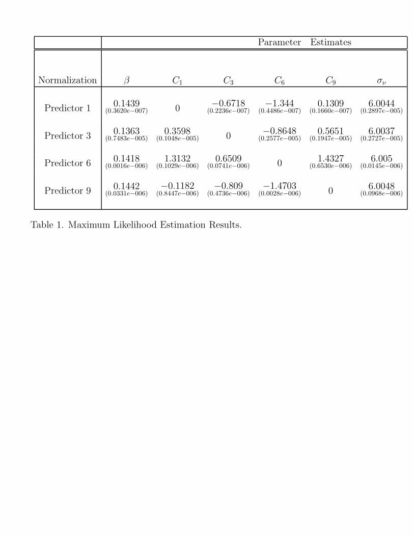
Parameter Estimates

Normalization β C1 C3 C6 C9 σν

Predictor 1 0.1439(0.3620e−007) 0

−0.6718(0.2236e−007)

−1.344(0.4486e−007)

0.1309(0.1660e−007)

6.0044(0.2897e−005)

Predictor 3 0.1363(0.7483e−005)

0.3598(0.1048e−005) 0

−0.8648(0.2577e−005)

0.5651(0.1947e−005)

6.0037(0.2727e−005)

Predictor 6 0.1418(0.0016e−006)

1.3132(0.1029e−006)

0.6509(0.0741e−006) 0 1.4327

(0.6530e−006)6.005

(0.0145e−006)

Predictor 9 0.1442(0.0331e−006)

−0.1182(0.8447e−006)

−0.809(0.4736e−006)

−1.4703(0.0028e−006) 0 6.0048

(0.0968e−006)

Table 1. Maximum Likelihood Estimation Results.

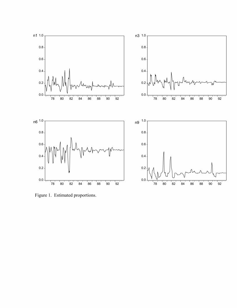
0.0

0.2

0.4

0.6

0.8

1.0

78 80 82 84 86 88 90 920.0

0.2

0.4

0.6

0.8

1.0

78 80 82 84 86 88 90 92

0.0

0.2

0.4

0.6

0.8

1.0

78 80 82 84 86 88 90 920.0

0.2

0.4

0.6

0.8

1.0

78 80 82 84 86 88 90 92

n1 n3

n6 n9

Figure 1. Estimated proportions.

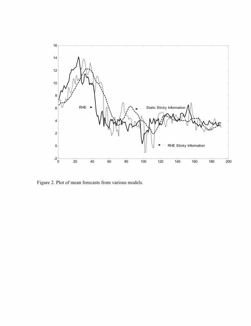
0 20 40 60 80 100 120 140 160 180 200-2

0

2

4

6

8

10

12

14

16

RHE Sticky Information

Static Sticky Information RHE

Figure 2. Plot of mean forecasts from various models.

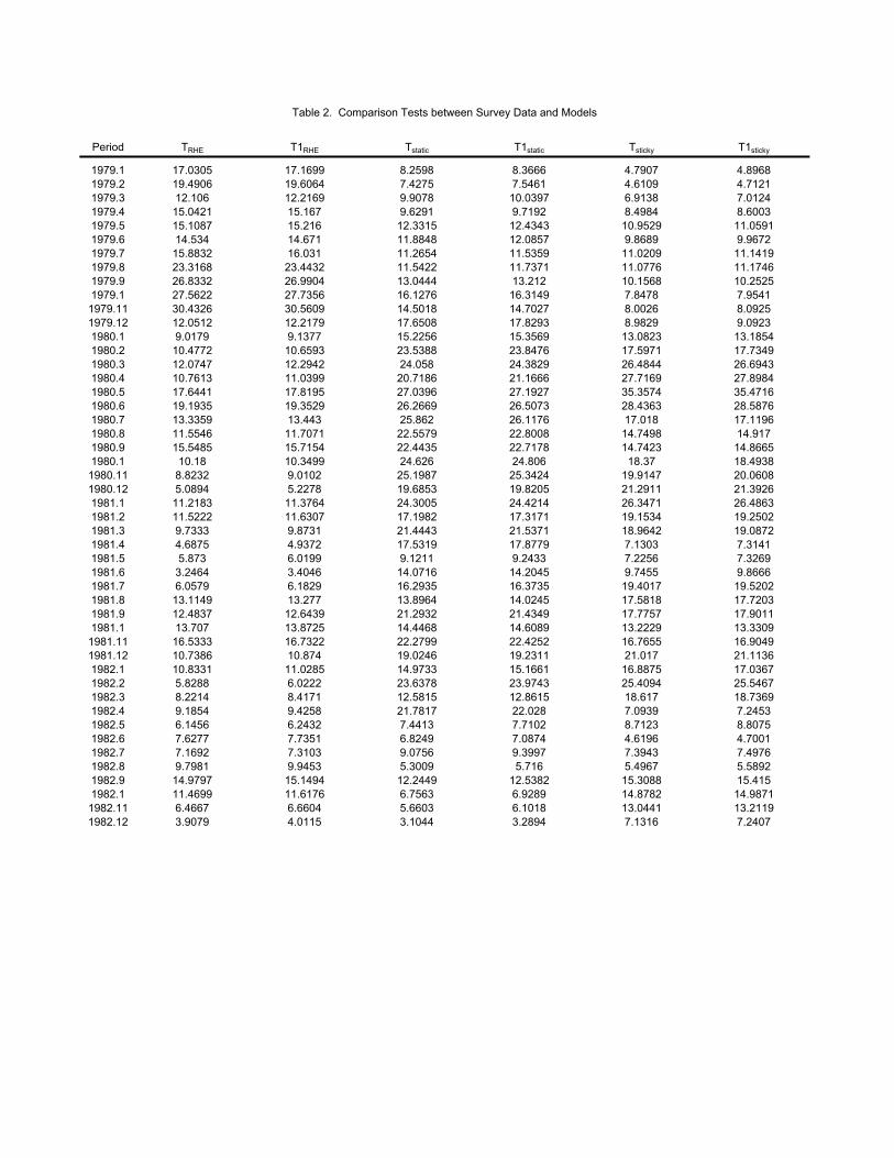
Period

1979.11979.21979.31979.41979.51979.61979.71979.81979.91979.11979.111979.121980.11980.21980.31980.41980.51980.61980.71980.81980.91980.11980.111980.121981.11981.21981.31981.41981.51981.61981.71981.81981.91981.11981.111981.121982.11982.21982.31982.41982.51982.61982.71982.81982.91982.11982.111982.12

Table 2. Comparison Tests between Survey Data and Models

15.41514.987113.2119

17.036725.546718.73697.2453

17.901113.3309

7.2407

8.80754.70017.49765.5892

16.904921.1136

7.32699.866619.520217.7203

26.486319.250219.08727.3141

14.866518.493820.060821.3926

35.471628.587617.119614.917

13.185417.734926.694327.8984

10.25257.95418.09259.0923

7.1316

T1sticky

4.89684.71217.01248.600311.05919.967211.141911.1746

5.496715.308814.878213.0441

7.09398.71234.61967.3943

21.01716.887525.409418.617

17.581817.775713.222916.7655

7.13037.22569.745519.4017

21.291126.347119.153418.9642

14.749814.742318.37

19.9147

27.716935.357428.436317.018

8.982913.082317.597126.4844

11.077610.15687.84788.0026

6.10183.2894

4.7907

Tsticky

4.61096.91388.498410.95299.868911.0209

9.39975.716

12.53826.9289

12.861522.0287.71027.0874

22.425219.231115.166123.9743

16.373514.024521.434914.6089

21.537117.87799.243314.2045

25.342419.820524.421417.3171

26.117622.800822.717824.806

24.382921.166627.192726.5073

14.702717.829315.356923.8476

11.535911.737113.21216.3149

3.1044

T1RHE Tstatic T1static

8.36667.546110.03979.719212.434312.0857

5.300912.24496.75635.6603

21.78177.44136.82499.0756

19.024614.973323.637812.5815

13.896421.293214.446822.2799

17.53199.121114.071616.2935

19.685324.300517.198221.4443

22.557922.443524.62625.1987

20.718627.039626.266925.862

17.650815.225623.538824.058

11.542213.044416.127614.5018

11.61766.66044.0115

8.25987.42759.90789.629112.331511.884811.2654

7.73517.31039.945315.1494

6.02228.41719.42586.2432

13.872516.732210.87411.0285

3.40466.182913.27712.6439

11.63079.87314.93726.0199

10.34999.01025.227811.3764

19.352913.44311.707115.7154

10.659312.294211.039917.8195

27.735630.560912.21799.1377

3.9079

17.169919.606412.216915.16715.21614.67116.03123.443226.9904

9.798114.979711.46996.4667

9.18546.14567.62777.1692

10.738610.83315.82888.2214

13.114912.483713.70716.5333

4.68755.873

3.24646.0579

5.089411.218311.52229.7333

11.554615.548510.18

8.8232

10.761317.644119.193513.3359

12.05129.017910.477212.0747

23.316826.833227.562230.4326

15.042115.108714.53415.8832

17.0305

TRHE

19.490612.106

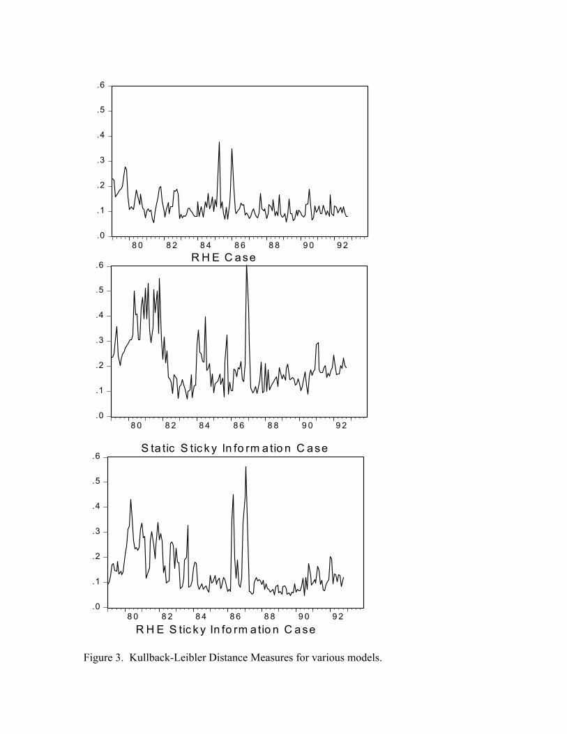
.0

.1

.2

.3

.4

.5

.6

8 0 8 2 8 4 8 6 8 8 9 0 9 2

.0

.1

.2

.3

.4

.5

.6

8 0 8 2 8 4 8 6 8 8 9 0 9 2

.0

.1

.2

.3

.4

.5

.6

8 0 8 2 8 4 8 6 8 8 9 0 9 2

R H E C ase

S ta tic S tic k y In fo rm a tio n C ase

R H E S tic k y In fo rm atio n C ase

Figure 3. Kullback-Leibler Distance Measures for various models.

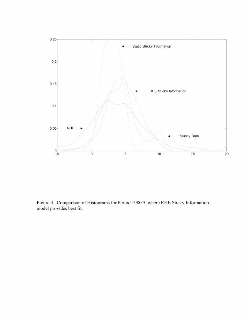
-5 0 5 10 15 200

0.05

0.1

0.15

0.2

0.25

Static Sticky Information

RHE Sticky Information

Survey Data

RHE

Figure 4. Comparison of Histograms for Period 1980.5, where RHE Sticky Information model provides best fit.

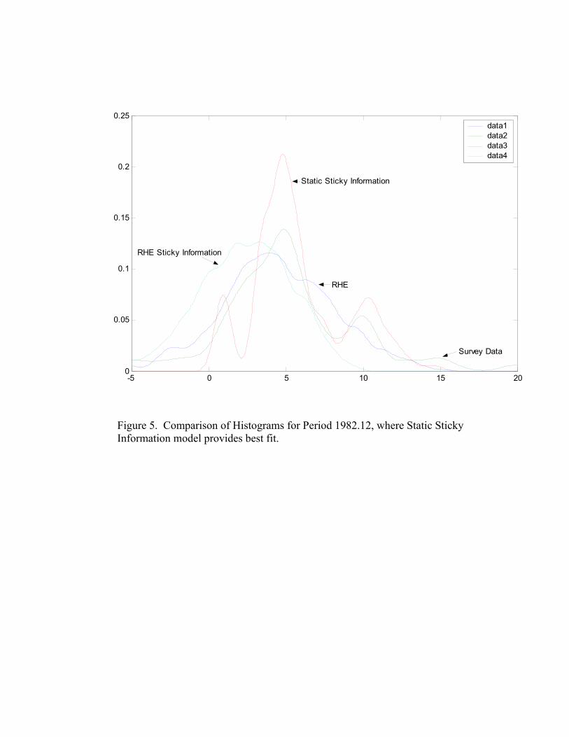
-5 0 5 10 15 200

0.05

0.1

0.15

0.2

0.25data1data2data3data4

RHE

Survey Data

Static Sticky Information

RHE Sticky Information

Figure 5. Comparison of Histograms for Period 1982.12, where Static Sticky Information model provides best fit.

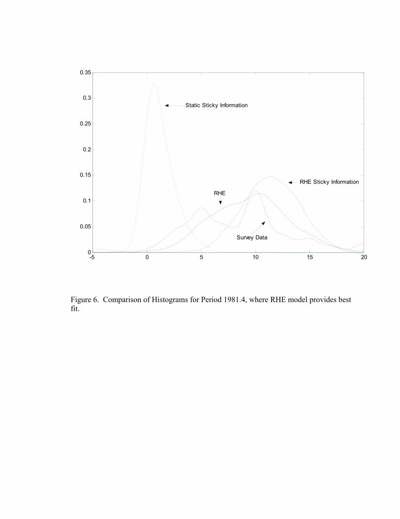
-5 0 5 10 15 200

0.05

0.1

0.15

0.2

0.25

0.3

0.35

Static Sticky Information

RHE Sticky Information

Survey Data

RHE

Figure 6. Comparison of Histograms for Period 1981.4, where RHE model provides best fit.

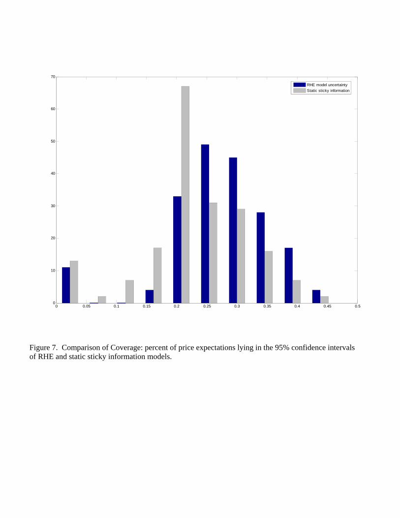
0 0.05 0.1 0.15 0.2 0.25 0.3 0.35 0.4 0.45 0.50

10

20

30

40

50

60

70

RHE model uncertaintyStatic sticky information

Figure 7. Comparison of Coverage: percent of price expectations lying in the 95% confidence intervals of RHE and static sticky information models.

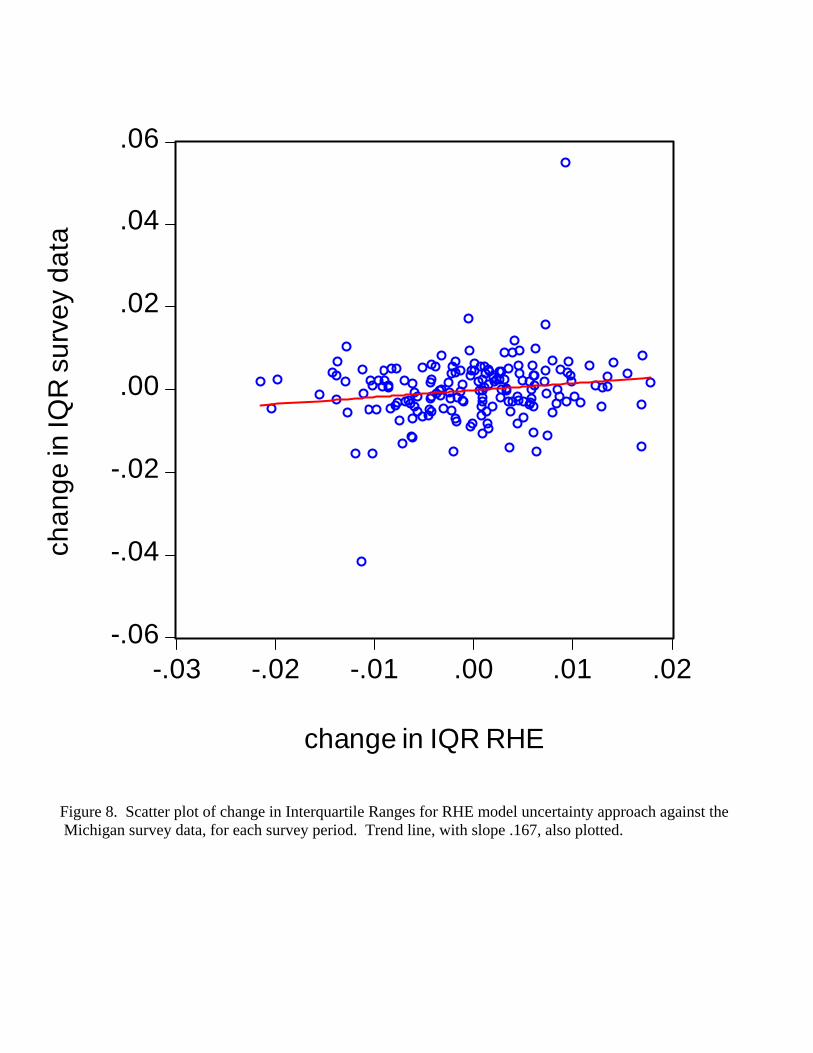
-.06

-.04

-.02

.00

.02

.04

.06

-.03 -.02 -.01 .00 .01 .02

change in IQR RHE

chan

ge in

IQR

sur

vey

data

Figure 8. Scatter plot of change in Interquartile Ranges for RHE model uncertainty approach against the

Michigan survey data, for each survey period. Trend line, with slope .167, also plotted.

-.06

-.04

-.02

.00

.02

.04

.06

-.08 -.04 .00 .04 .08

change in IQR static sticky info

Cha

nge

in IQ

R s

urve

y da

ta

Figure 9. Scatter plot of changes in Interquartile Ranges for static sticky information approach against the

Michigan survey data, for each survey period. Trend line, with slope .0099, also plotted.

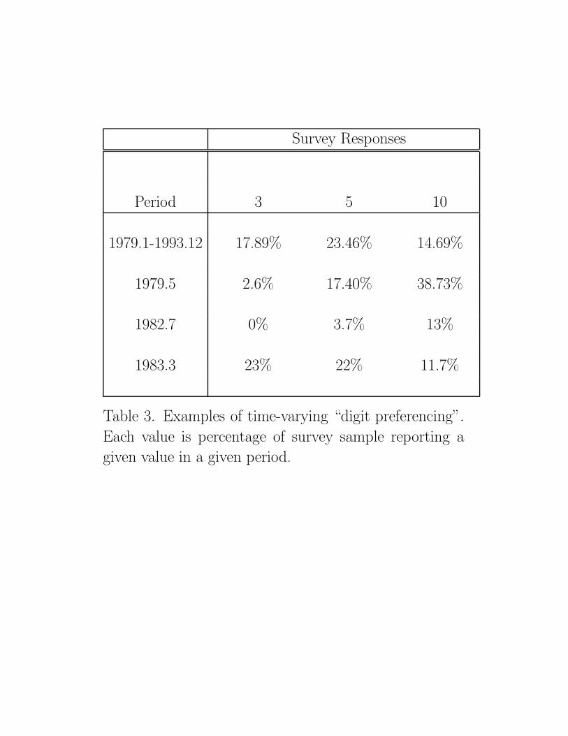
Survey Responses

Period 3 5 10

1979.1-1993.12 17.89% 23.46% 14.69%

1979.5 2.6% 17.40% 38.73%

1982.7 0% 3.7% 13%

1983.3 23% 22% 11.7%

Table 3. Examples of time-varying “digit preferencing”.

Each value is percentage of survey sample reporting a

given value in a given period.

1 2 3 4 5 6 7 8 9 10 11 120

5

10

15

20

number of peaks in distribution of survey data

frequ

ency

1 2 3 4 5 6 7 8 9 10 11 120

5

10

15

20

number of peaks in distribution of RHE-model uncertainty

frequ

ency

1 2 3 4 5 6 7 8 9 10 11 120

5

10

15

20

number of peaks in distribution of static sticky information

frequ

ency

1 2 3 4 5 6 7 8 9 10 11 120

10

20

30

40

50

60

number of peaks in distribution of survey data

frequ

ency

1 2 3 4 5 6 7 8 9 10 11 120

10

20

30

40

50

60

number of peaks in distribution of RHE-model uncertainty

frequ

ency

1 2 3 4 5 6 7 8 9 10 11 120

10

20

30

40

50

60

number of peaks in distribution of static sticky information

frequ

ency

1979.1-1982.12 1979.1-1993.12

Figure 10. Plots the number of peaks in the distributions of survey data, density functions of RHE-model uncertainty and static sticky information. The left column of histograms plots the number of peaks in a given time-period’s distribution over the period 1979.1-1982.12. The right column plots the number of peaks in a given time period’s distribution over the period 1979.1-1993.12.