Sticky information and model uncertainty in survey …wbranch/Templates/stickyinfojedcpub.pdf ·...

ARTICLE IN PRESS

Journal of Economic Dynamics & Control 31 (2007) 245–276

0165-1889/$ -

doi:10.1016/j

�Tel.: +1 9

E-mail ad

www.elsevier.com/locate/jedc

Sticky information and model uncertainty insurvey data on inflation expectations

William A. Branch�

Department of Economics, 3151 Social Science Plaza, Irvine, CA 92697, USA

Received 7 July 2005; accepted 11 November 2005

Available online 15 March 2006

Abstract

This paper compares three reduced-form models of heterogeneity in survey inflation

expectations. On the one hand, we specify two models of forecasting inflation based on limited

information flows of the type developed in Mankiw and Reis [2002. Sticky information versus

sticky prices: a proposal to replace the new Keynesian Phillips curve. Quarterly Journal of

Economics 117(4), 1295–1328]. We present maximum likelihood results that suggests a sticky

information model with a time-varying distribution structure is consistent with the Michigan

survey of inflation expectations. We also compare these ‘sticky information’ models to the

endogenous model uncertainty approach in Branch [2004. The theory of rationally

heterogeneous expectations: evidence from survey data on inflation expectations. Economic

Journal 114, 497]. Non-parametric evidence suggests that models which allow the degree of

heterogeneity to change over time provide a better fit of the data.

r 2006 Elsevier B.V. All rights reserved.

JEL classification: C53; C82; E31; D83; D84

Keywords: Heterogeneous expectations; Adaptive learning; Model uncertainty; Survey expectations

see front matter r 2006 Elsevier B.V. All rights reserved.

.jedc.2005.11.002

49 824 4221; fax: +1 949 824 2182.

dress: [email protected].

www.elsevier.com/locate/jedc

dx.doi.org/10.1016/j.jedc.2005.11.002

mailto:[email protected]

ARTICLE IN PRESS

W.A. Branch / Journal of Economic Dynamics & Control 31 (2007) 245–276246

1. Introduction

Despite the prominence of rational expectations in macroeconomics there isconsiderable interest in its limitations. Recent approaches impose boundedrationality at the primitive level; see, for example, Mankiw and Reis (2002), Ballet al. (2005), Reis (2004), Branch et al. (2004) and Sims (2003). Of these the stickyinformation model of Mankiw and Reis (2002) yields important (and tractable)implications for macroeconomic policy. Mankiw and Reis (2002) replace thestaggered pricing model of Calvo (1983), which is employed extensively in Woodford(2003), with a model of staggered information flows. Each period, each firm, with aconstant probability, updates its information set when optimally setting prices. Theremaining firms are free to set prices also, but do not update their information fromthe previous period.

This paper has three objectives: first, to characterize sticky information in surveydata in the sense that a proportion of agents do not update information each period;second, to test whether these proportions are static or dynamic; third, compare howwell three competing reduced-form models of expectation formation fit the surveydata. Carroll (2003) and Mankiw et al. (2003) provide indirect evidence of limitedinformation flows in expectation formation. This paper elaborates on the nature ofthese flows in survey data. We also bridge the sticky information and heterogeneousexpectations literature by presenting evidence of both model heterogeneity andlimited information flows.

There is considerable interest in empirically inferring the methods with whichagents form expectations. In particular, there is compelling evidence that surveyexpectations are heterogeneous and not rational. In an innovative paper, Mankiw etal. (2003) seek evidence of sticky information in survey data on inflationexpectations. They examine surveys of professional forecasters and construct a dataset based on the Michigan Survey of Consumers. Their results show that these surveydata are inconsistent with either rational or adaptive expectations and may beconsistent with a sticky information model. Bryan and Venkatu (2001a, b) documentstriking differences in survey expectations across demographic groups. Carroll(2003) provides evidence that the median response in the Survey of Consumers is adistributed lag of the median response from the Survey of Professional Forecasters.Branch (2004), adapting Brock and Hommes (1997), develops a methodology forassessing the forecasting models agents use in forming expectations. In that paper,evidence suggests survey responses are distributed heterogeneously across univariateand multivariate forecasting models. Brock and Durlauf (2004) argue that if agentsare uncertain about the prevailing inflation regime then this uncertainty maymanifest itself in agents switching between myopic and forward-looking predictors;hence, model uncertainty may be an aspect of expectation formation.1

1Other papers which show heterogeneity across forecasting models include Baak (1999), Chavas (2000),

and Aadland (2004). Experimental evidence is provided by Heemeijer et al. (2004) and Hommes et al.

(2005).

ARTICLE IN PRESS

W.A. Branch / Journal of Economic Dynamics & Control 31 (2007) 245–276 247

This paper extends Branch (2004) by enlarging the set of competing reduced formmodels. Our approach, like Mankiw et al. (2003), tests for a particular form of stickyinformation flows in agents’ survey expectations. We also extend Mankiw et al.(2003) by proposing two formulations of sticky information. The first is theMankiw–Reis approach which we refer to as the static sticky information model. Reis(2004), in a microfounded model of inattentiveness, shows that with costly updatingof information firms may choose to be inattentive, and under certain conditions thedistribution of information may be in line with Mankiw–Reis. Motivated by Reis’purposeful model of inattention, the other approach assumes that expectations areformed by a discrete choice between forecasting functions which differ by thefrequency with which they are recursively updated. Using data from the Survey ofConsumers at the University of Michigan, we provide evidence of sticky informationby testing the reduced-form sticky information models against the full-informationalternative. Maximum likelihood evidence shows that: sticky information in surveydata is dynamic in the sense that the distribution of agents across predictors is time-varying; the distribution of agents is not geometric so that, on average, the highestproportion of agents update information somewhat infrequently. This last result is incontrast to an implication of the Mankiw–Reis model which has the highestproportion of agents updating each period.

Our final objective is to compare these models with the approach presented inBranch (2004). In Branch (2004) agents make a discrete choice between (non-nested)alternatives.2 We (non-parametrically) estimate the density functions implied bythese models and compare the fit to the histogram of the actual survey data. We findthat neither the sticky information or the model uncertainty reduced-formapproaches are statistically identical to the distribution of the survey data. Weshow, however, that a sticky information model which lets the distribution ofinformation across agents vary over time provides a better fit than the static versionof Mankiw and Reis (2002).

In this last empirical exercise, we use non-parametric techniques to assess how welleach model fits the entire period by period distribution of survey expectations. Sinceit is not reasonable to expect that the simple empirical models, motivated by theory,will provide an exact match to the data, we examine how closely they can track theevolution across time of the central tendencies and dispersion of survey expectations.Our results suggest that the model uncertainty and sticky information theories, witha time-varying distribution of agents across models, capture the time-variationreasonably well. This paper’s aim is to, at a first pass, assess to what degree thetheoretical models can explain the primary dynamics of survey expectations.

Our results suggest that a structural approach to model uncertainty andinattentiveness along the lines of Reis (2004) may further enhance our understandingof the process of expectation formation. It is important to note, then, that ourresults are specific to classes of expectation formation models. Our approachprevents us from making more general statements about all classes of models ormaking broader structural claims about model uncertainty or inattentiveness.

2Pesaran and Timmermann (1995) also find evidence of model uncertainty.

ARTICLE IN PRESS


Although the theoretical models of expectation formation do not provide a perfectfit, we argue that they capture important characteristics of the survey data. Theresults here provide the first empirical comparison of heterogeneous expectationsmodels.

This paper proceeds as follows. In Section 2 we present the three expectationformation models. Section 3 discusses the maximum likelihood results. Section 4compares the fit of the heterogeneous expectations models to the distribution ofsurvey responses. Finally, Section 5 concludes.

2. Two models of sticky information

Our methodology compares three alternative models of expectation formation tosurvey data on inflation expectations.3 The first two are models of stickyinformation: first, the Mankiw and Reis (2002) model of sticky information; second,a discrete choice model of sticky information inspired by Brock and Hommes (1997).The third approach is the model uncertainty case of Branch (2004).4

2.1. Survey expectations

This paper characterizes the 12-month ahead inflation expectations in theMichigan survey. The data come from a monthly survey of approximately 500households conducted by the Survey Research Center (SRC) at the University ofMichigan. The results are published as the Survey of Consumer Attitudes andBehavior and in recent years as the Survey of Consumers. This paper uses the data inBranch (2004), which covers the period 1977.11–1993.12, because it covers a diversespectrum of inflation volatility (e.g. great inflation and great moderation) and tokeep the comparison sharp with our earlier work.5 This paper characterizesexpectations of future inflation6 and the sample consists of 93 142 observationscovering 187 time periods. The mean response was 6.9550 with a standard deviationof 12.7010. The large standard deviation is accounted for by a few outliers thatexpect inflation to be greater than 40%. Excluding these responses does not changethe qualitative results. Mankiw et al. (2003) extend the sample to prior periods byinferring a distribution from the survey sample.

3Three is a sufficient number of approaches because one of the models was shown by Branch (2004) to

fit survey data better than other alternatives including rational expectations. Thus, the approaches here

encompass the classes of forecasting models employed most frequently in the literature.4We use the terms sticky information and model uncertainty as descriptors of the reduced-form models.

The underlying micro behavior which leads to these empirical models is not implied by these terms.5There are some missing months in 1977, and so the sample is restricted only to continuous periods.6The two relevant questions are:

1. During the next 12 months, do you think that prices in general will go up, down, or stay where they are

now?

2. By about what percent do you expect prices to go (up/down) on the average, during the next 12

months?

ARTICLE IN PRESS


In the Michigan survey each agent i at each date t reports their 12-month aheadforecast ~pe

i;t. We assume that agents estimate a VAR of the form,

yt ¼ A1;t�1yt�1 þ � � � þ Ap;t�1yt�p þ et,

which has the VAR(1) form,

zt ¼ At�1zt�1 þ ~et, (1)

where zt ¼ ðyt; yt�1; . . . ; yt�pþ1Þ0 and ~et is iid zero mean. If yt consists of n variables

then zt is ðnp� 1Þ and A is ðnp� npÞ. The specification and estimation of theparameters of the model are discussed below.

Notice that in (1) we allow agents to estimate a VAR with time-varyingparameters. This is in accordance with the adaptive learning literature whereagents, uncertain about the true value of A, estimate At�1 in real-time. Then (1)could also be a particular theory of model uncertainty. Below, we are interested inhow survey expectations are distributed across several variants of this model. Wenow turn to specifying sticky information within the context of this VAR forecastingmodel.

One point is worth stating here: because these expectations are phrased by thesurveyor as 12-month ahead forecasts, we assume agents look at past monthlyinflation to forecast 12-month ahead inflation. In other words, the VAR in (1)consists of monthly data. This assumption is also made in Mankiw et al. (2003).7

2.2. Static sticky information

In a series of papers, Mankiw and Reis (2002), Ball et al. (2005), and Mankiw et al.(2003) introduce a novel information structure to expectation formation. Unlikemuch of the bounded rationality literature they assume that agents have thecognitive ability to form conditional expectations (i.e. rational expectations).However, each agent faces an exogenous probability l that they will update theirinformation set each period. It is important to stress that in the Mankiw–Reisapproach expectations are not static; those agents who do not update theirinformation sets still update their expectations.

Define I t�j as the information set of an agent who last updated j periods ago; theset I t�j consists of all explanatory variables dated t� j or earlier. Using the VARforecasting model (1), an agent who last updated j periods ago will form, in time t, atwelve-step ahead forecast of monthly inflation using all information availablethrough t� j. Under these timing assumptions j ¼ 0 is equivalent to full-information.8 Full information in this setting is not complete information since (1)is a reduced-form VAR that could represent model uncertainty (because of the time-varying parameters). In order to form this forecast the agent must generate a series

7The Labor Department in its press release reports first the monthly inflation figure. Thus, it is not

unreasonable to assume it is an input to agents’ forecasting model.8Of course, because we have not posed a model for the economy these expectations may not be rational.

Instead, at best these are the optimal linear forecasts given beliefs in (1). In the terminology of Evans and

Honkapohja (2001) these are restricted perceptions.

ARTICLE IN PRESS


of i-step ahead forecasts of monthly inflation,

pej;tþi ¼ EðptþijI t�jÞ ¼ ðA

jþit�jzt�jÞp,

where ðAjþit�jzÞp is the inflation component of the projection, with p denoting monthly

inflation.9 The agent then continues out-of-sample forecasting in order to generatethe sequence pe

j;tþ1;pej;tþ2; . . . ;p

ej;tþ12. The 12-month ahead forecast of annual inflation

is generated according to,

pj;tþ12 ¼X12i¼1

pej;tþi.

It is worth emphasizing the forecasting problem facing agents. Agents estimate aVAR that consists of monthly data. Information arrives stochastically, and so giventhe most recent information agents forecast annual inflation by iterating theirforecasting model ahead j þ 12 periods.

Given the exogenous probability of updating the information sets, a proportion lof agents update in time t. Thus, at each t there are l agents with p0;tþ12, lð1� lÞwith p1;tþ12, lð1� lÞ2 with p2;tþ12, and so on. The mean forecast is,

petþ12ðlÞ ¼ l

X1j¼0

ð1� lÞjpj;tþ12.

Reis (2004) shows that, in a model where firms face costly updating of information, itis possible that aggregate inattentiveness could also yield this reduced-form. Below,in our empirical approach, we will sample from this sticky information distributionto generate a predicted survey sample and assess this model’s ability to explain theentire distribution of Michigan survey responses.10

2.3. Rationally heterogeneous sticky information

The Mankiw–Reis approach in the previous subsection is a reduced-formheterogeneous expectations model with a geometric distribution of expectationssimilar to the Calvo-style pricing structure emphasized in Woodford (2003). Thereare other heterogeneous expectations models. For instance, the seminal approach ofBrock and Hommes (1997) can be applied to ascertain whether agents are distributedacross predictors which differ in dimension of the zt in (1).

This subsection presents a rationally heterogeneous expectations (RHE) extensionof Branch (2004) to limited information flows. We assume agents are confronted

9The implicit assumption in this projection is that agents assume A remains constant over the forecast

horizon. An interesting extension would be to consider a setting where agents account for their uncertainty

in A when constructing conditional forecasts.10In Branch and Evans (2005), a recursively estimated VAR is used to forecast inflation and GDP

growth and then these forecasts are compared to the SPF. A VAR forecast is found to fit well. We

conjecture that replacing the VAR forecasts with the SPF, as in Carroll (2003), will not alter the qualitative

results below.

ARTICLE IN PRESS


with a list of forecasting models distinct in the frequency of recursive updating. Ineach period agents choose their expectations from this list. This approach can beviewed as a reduced-form generalization of Reis (2004). Reis’ model is a firstprincipled alternative to Mankiw–Reis in the sense that the choice of updatingprobabilities is purposefully chosen and (possibly) time-varying. One could envisionthe reduced-form in this paper as arising from Reis’ model extended to includestructural change.

There is a burgeoning literature on dynamic predictor selection. A prime exampleis the adaptively rational equilibrium dynamics (ARED) of Brock and Hommes(1997). In the ARED the probability an agent chooses a certain predictor isdetermined by a discrete choice model. There is an extensive literature which modelsindividual decision making as a discrete choice in a random utility setting (e.g.Manski and McFadden, 1981). The proportion of agents using a given predictor isincreasing in its relative net benefit.

Let Ht ¼ fpj;tþ12g1j¼0 denote the collection of predictors with information sets

updated j periods ago. The static information alternative in the previous subsectiongenerates mean responses by placing a geometric structure on the components ofHt.In the alternative approach we assume that there are a finite number of elements inHt.

11 Moreover, unlike in the previous subsection, we assume that each predictorpj;tþ12 is recursive and updated each ðj þ 1Þ periods.12 It should be noted that thepredictors are updated each j þ 1 periods since j ¼ 0 was designated above as full-information.13 This differs from Mankiw–Reis in that the RHE approach no longerassumes expectations are rational; it imposes that agents ignore information thatagents in Mankiw–Reis’ approach would not. Although we defend this assumptionbelow, we leave which approach is a better reduced-form model as an empiricalquestion.

Let Uj;t denote the relative net benefit of a predictor last updated j þ 1 periods agoin time t. We define Uj;t in terms of mean square forecast error. The probability anagent will choose predictor j is given by the multinomial logit (MNL) map

nj;t ¼exp½bUj;t�Pk exp½bUk;t�

. (2)

The parameter b is called the ‘intensity of choice’. It governs how strongly agentsreact to relative net benefits. The neoclassical case has b ¼ þ1 and nj;t 2 f0; 1g. Ourhypothesis is that b40. Implicitly, Mankiw et al. (2003) impose the restrictionbUj;t ¼ U j ; 8t. Our approach allows us to test this restriction. It is worthemphasizing that (2) is a (testable) theory of expectation formation. It formalizes

11Brock et al. (2005) introduce the idea of a large-type limit (LTL) model of discrete predictor choice. In

the LTL model there are an infinite number of predictors. We note that their approach is beyond the scope

of this paper.12In the static case, pj;tþ12 is a ðj þ 12Þ step ahead out of sample forecast. As an alternative we allow

updating in pj;tþ12.13Below we will change this (unfortunate) notation so that j is descriptive and represents the frequency

with which the predictor is updated.

ARTICLE IN PRESS


the intuitively appealing assumption that the proportion of agents using a predictoris increasing in its accuracy.14

It is standard in the adaptive learning literature to assume that past forecast erroris the appropriate measure of predictor fitness. The motivation is to treat theexpectation formation decision as a statistical problem. In such settings mean-squareforecast error is a natural candidate for measuring predictor success. Moreover, solong as predictor choice reinforces forecasting success, then alternative measures offitness will not change the qualitative results.

The RHE approach has the advantage over the Mankiw–Reis model that it doesnot a priori impose the structure of heterogeneity. Rather than a stochasticinformation gathering process, here the process is purposeful.15 In this approachagents may switch between models with full information to models with datedinformation which implies agents may forget what they learned in the past. Thisstructure is justified, though, since in the RHE approach each predictor is recursivelyre-estimated every j periods given recent data. If information gathering is costly thenan agent may only incorporate the most recent data point when going from aninfrequently updated to a frequently updated predictor. When going from afrequently updated to a less frequently updated predictor, though, it appears thetheory imposes that agents dispose of useful information. However, this is logicallyconsistent if one thinks of consumers forming expectations via ‘market consensus’forecasts published in the newspaper – agents have acquired the forecast but not theforecasting method, thereby, not disposing of important information themselves. Afully specified model would also allow agents to choose, each period, how much‘memory’ they have. This is intractable in the current framework and we leave thisissue to future research.

2.4. Model uncertainty

Rather than examining heterogeneity in information updating, Branch (2004)examines heterogeneity in VAR dimensions. Specifically, suppose that agents choosefrom a set which consists of a VAR predictor, a univariate adaptive expectationspredictor, and a univariate naive predictor. We interpret model uncertainty as agentsselecting from the set Ht ¼ fVARt;AEt;NEtg where VARt is identical to the full-information forecast in the static sticky information model, AEt is an adaptiveforecast of the form

AEt ¼ ð1� gÞAEt�1 þ gpt�1,

where g ¼ :216, and NEt ¼ pt�1 is the naive forecast. Agents are distributed acrossthese predictors according to the MNL (2).

This theory restricts the set of predictors to VARt;AEt;NEt, which arerepresentative of the most commonly used models of expectation formation. This

14The theory assumes that the forecast benefits are identical across individuals. A relaxation of this

assumption is beyond the scope of this paper and is the subject of future research.15Up to the noise in the random utility function.

ARTICLE IN PRESS


set of predictors is meant to represent the classes of multivariate and univariateforecasting methods. Branch (2004) shows how heterogeneity across these models fitsthe data well in comparison to alternatives. One goal of this paper is to extend the setof alternatives to include sticky information predictors that are not special cases ofthe model uncertainty case.

Our use of the term ‘model uncertainty’ may seem non-standard. Modeluncertainty is typically expressed as ambiguity over the correct structural modelfor the economy, the Fed’s interest rate rule, etc. Here model uncertainty is expressedas a forecasting problem: given costly estimation, what is the ideal forecasting model.This choice is not trivial in practice: the forecast advantage of a VAR or adaptivepredictor relative to naive depends on the time period. The typical definition andours are congruent, however, as switching between forecast models is meant to proxyfor an underlying, deeper sense of model uncertainty. Because the RHE modeluncertainty alternative is meant as a representation of more fundamental behavior,we cannot interpret poor empirical fit as an indictment against all forms of modeluncertainty.

3. Empirical results

This section presents results of an empirical analysis of the two sticky informationmodels in comparison to the survey data on inflation expectations.

3.1. Predictor estimation

We begin this section with a description of how we constructed the predictorfunctions. The construction follows the steps: first, specification of the VAR andvector of explanatory variables zt; second, a description of predictor functions in thetwo sticky information alternatives; third, we describe a process of recursiveforecasting.

First, we describe the VAR which is the basis for forecasting.16 We follow Branch(2004) and Mankiw et al. (2003) in assuming that the VAR(1) consists of monthlyinflation, unemployment, and 3-month t-bill rates. A VAR with this set of variablesis parsimonious and forecasts inflation well. Our metric for forecast comparison issquared deviations from actual annual inflation. We choose a lag length of 12 inorder to minimize the Akaike Information Criterion. This VAR is used to generate a12-month ahead forecast of inflation.

There are several issues to pin down. The model of sticky information presented inthis paper is an assumption on the information sets, which evolve stochastically.Each sticky information alternative makes specific assumptions on how agents’information sets evolve. However, the parameters of the VAR model may be time-varying and unknown by agents. As a result, we assume that when agents update

16We focus on VAR forecasting because it is often cited as an approximation to rational expectations

and is a frequently employed forecasting strategy.

ARTICLE IN PRESS


their information they also update their estimates of the model’s parameters.Because these issues are distinct from our earlier paper, this subsection discussespredictor estimation at length.

In the Mankiw–Reis model we assume that l agents have forecasts based on themost recently available data, lð1� lÞ have two-step ahead out of sample forecastsbased on the most recently available data from two periods ago, and so on. Toconstruct the Mankiw–Reis forecasts we recursively generate a vector of out ofsample forecasts. We then weight and sum these forecasts as described in theprevious section. To test this model against the survey data we generate randomdraws from the distribution implied by this information structure and then comparethe densities of these draws to the histogram of the actual survey data. Below wediscuss how parameter estimates are updated in this context. We follow Mankiw etal. (2003) by fixing l ¼ :1. To ensure robustness of our results, we also let:05plp:25.17 All qualitative results are robust to values of l in this range.

In order to formulate a tractable empirical model of dynamic predictor selectionwe must impose bounds on Ht. At this point we make a notational change whichwill ease exposition. In the previous section, j ¼ 0 denoted full-information. To stressthat in the RHE setting full-information is equivalent to updating every period wenow denote p1 as the predictor updated each period. We assume that

Ht ¼ fp1;tþ12; p3;tþ12; p6;tþ12; p9;tþ12g.

That is, the available predictors update information every period, every third period,every sixth period, and once every nine periods. We make these restrictions in orderto maximize the number of identifiable predictors. We omit VARs estimated everyother period, every fourth period, and so on, because they produce forecasts tooclosely related to the predictors in Ht.

We also omit VARs estimated less frequently than every 9 months. VARsestimated every 12 (or 24) months will produce forecasts similar to the 9 monthpredictor and our estimation strategy will not be able to separately identify agentswith a 9 or 12 month predictor.18 It is important to note that this bound does notaffect the qualitative results. An advantage to the empirical procedure below is it willidentify those agents that update less than once a year as p9 which still implies ‘stickyinformation’ in this context.

Given a method for updating the models in Ht and the discrete choice mechanism(2), all that is needed to make the RHE sticky information model well-defined is apredictor fitness measure,

Uj;t ¼ �ðpt�1 � pj;t�1Þ2� Cj � �MSEj;t � Cj, (3)

17It is straightforward to choose a l which minimizes the distance, in a measure-theoretic sense, between

the density of the actual data with that of the Mankiw–Reis density (which is a function of l). Empirical

exploration suggests that the optimal l falls in the range ½:05; :25� based on minimizing a Kullback–Leibler

distance measure. A smaller value of l (.05) is preferred if the objective is to minimize the total distance

from the actual data and a larger value (.25) if minimizing the mean distance across periods is the goal.18This follows because to construct forecasts on 9 or 12 month predictors we are iterating a VAR whose

parameter matrix has eigenvalues inside the unit circle.

ARTICLE IN PRESS


where Cj is a constant around which the mean predictor proportions vary. Agentsare assumed to base decisions on how well a given predictor forecasted the mostrecent annual inflation rate. In Brock and Hommes (1997), Cj plays the role of a cost;predictors with higher computation or information gathering costs will have a largerCj . However, the theory itself is more flexible and the Cj’s may actually pick uppredisposition effects. Essentially, the Cj ensure that the empirical estimates of theproportions of agents most closely fits the data. The Cj act as thresholds throughwhich forecast errors must cross to induce switching, by agents, between predictionmethods. This role for the constants is consistent with the role of costs in Brock andHommes (1997) and is discussed in detail in Branch (2004). We note briefly thatpredictors estimated more frequently produce lower mean square errors, however, inany given period a sticky information predictor could produce a lower forecast error.

A brief justification of the form of (3) is warranted. While mean-square error as ametric for forecasting success is motivated by theory, the weighting of past data inthe MSE measure is an empirical question. We use only the most recent forecasterror not as an ad hoc assumption for convenience, but because preliminaryexplorations indicated it provided the best fit for the sticky information model. It isworth noting that in our earlier paper we assumed a geometric weighting on the pastsquared errors in the RHE model uncertainty approach.

We now describe how the forecasts are actually computed. We assume agentsengage in real-time learning by recursively updating their prior parameterestimates.19 In VARs with time-varying parameters and limited samples, recursiveestimation is desirable. Our approach is a straightforward extension of Stock andWatson (1996) to a setting where the parameters are updated periodically with themost recent data point. Each forecast function differs in how often it recursivelyupdates its parameter estimates. This approach is motivated by costly informationgathering that induces agents to sample recent data periodically and to update theirprior parameter estimates at the time of sampling.

The full VAR zt is estimated according to

zt ¼ At�1zt�1 þ ~et,

where

At ¼ At�1 þ t�1R�1t zt�1ðz0t � z0t�1A

0t�1Þ,

Rt ¼ Rt�1 þ t�1ðzt�1z0t�1 � Rt�1Þ.

Note that Rt is the sample second moment of zt�1.20 Since there are three variables

and 12 lags, the vector zt is ð36� 1Þ and At is ð36� 36Þ. These recursions constituterecursive least squares (RLS). Each predictor is a VAR whose parameter estimatesare generated at different frequencies. In the static sticky information alternativeonly l agents have these expectations, while lð1� lÞj form projections based onAt�j�1.

19Some authors advocate forecasting based on real-time data sets (see Croushore and Stark, 2003). Such

an undertaking is beyond the scope of this paper.20See Evans and Honkapohja (2001) for an overview of real-time learning using recursive least squares.

ARTICLE IN PRESS


One (potential) concern is that because of the great moderation – and otherstructural changes after 1960 as pointed out by Sims and Zha (2005) – inflation is notstationary and our VAR forecasting model may under predict inflation in the earlyyears and over predict in later years. The recursive forecasting approach addressesthis concern by allowing for time-varying parameters which remain alert to possiblestructural change.

For the RHE sticky information model, denote zj;t as the VAR updated every j

periods. Each restricted VAR zj;t is updated every jth period according to,

Aj;t ¼Aj;t�1 þ t�1R�1j;t zj;t�1ðz

0t � z0j;t�1A

0j;t�1Þ every jth t;

Aj;t�1 otherwise:

(

A similar updating rule exists for Rj;t as well. The term t�1 defines a decreasing gainsequence since it places lower weight on recent realizations. Some recent models withlearning emphasize recursive estimates generated with a constant gain sequenceinstead. By replacing t�1 with a constant, a greater weight is placed on recentrealizations than distant ones. We note that our results are robust to RLS parameterestimates generated by a constant gain algorithm. Given an estimate for Aj;t a seriesof 12 one-step ahead forecasts are formed, just as in the static sticky informationalternative, to generate a forecast of annual inflation.

In the estimation we set the initial parameter estimates equal to its least squaresestimates over the period 1958.11–1976.10. From 1976.11 onwards each predictorupdates its prior parameter estimates every j periods. This implies that the parametermatrices A1;t;A3;t;A6;t;A9;t will be different across all t41976:11. Implicit in theRHE specification of sticky information is that when agents update information theyonly acquire the most recent data point. A downside is that as agents switch frommodels that are updated frequently to those that are updated infrequently agents willbe disposing of information acquired in previous periods. As mentioned above, thisis logically consistent if agents are boundedly rational in the sense that they chooseforecasts, pj;t, from a set of alternatives Ht.

3.2. Discussion of forecasting models

Forecasts based on VARs like (1) are employed extensively in macroeconomics.One might also ask why agents do not just adopt professionals’ forecast. Ourapproach is consistent with this alternative if professionals adopt a VAR forecastingapproach. One (possible) objection to the theory of RHE model uncertainty is thatagents should use Bayesian model averaging to deal with their uncertainty. We donot allow for a ‘model-averaged’ predictor because the theory assumes that thechoice made by agents is how sophisticated of a model they should employ given thatexpectation calculation is costly. Bayesian model averaging is another step in thesophistication and it should not alter our results.

It is important to note that the results in this section are conditional on particularclasses of reduced-form models. We consider three classes: a static sticky informationmodel with a geometric distribution of agents; a discrete choice sticky information

ARTICLE IN PRESS


model; and multivariate and univariate forecasting models. Branch (2004) showedthat the RHE model uncertainty case fits the data better than alternatives such asfull-information VAR expectations, rational and adaptive expectations, and othermyopic expectation formation models. Thus, our results extend the earlier paper tothese two additional models. Our results do not extend to classes of modeluncertainty or sticky information not considered here. Because the models arereduced-form it is not possible to draw structural conclusions from the empiricalresults. A time-varying VAR for example could represent uncertainty about thestructural model parameters. Univariate forecasting models, on the other hand,could arise from a model where agents are ‘inattentive’ to other factors, such asoutput growth.

Although the sample length of the survey data is 1977.11–1993.12, we follow Stockand Watson’s out-of-sample forecasting approach and initialize the VAR over1958.11–1977.10, thus ensuring our results are not sensitive to choice of gainsequence (see Branch and Evans, 2005).

3.3. Maximum likelihood estimation of RHE sticky information model

In this subsection we address the paper’s primary objective: to test for dynamicsticky information and to estimate the distribution of agents across predictors. Weachieve the first objective by testing H0 : b40, the second objective is achieved byestimating the hierarchy of the Cj ; j ¼ 1; 3; 6; 9. First, a brief discussion of theestimation approach.

Although the predictors are different in the RHE sticky information and RHEmodel uncertainty cases, the specification of the econometric procedure, below, isbased on Branch (2004). The theory predicts that survey responses take a discretenumber of values; namely, there are only four possible responses. However, thesurvey itself is continuously valued. To this end, we specify a backwards MNLapproach. Each survey response is assumed to be reported as

~pei;t ¼ pj;tþ12 þ ni;t, (4)

where ni;t is distributed normally and j 2 f1; 3; 6; 9g. A survey response is a 12-monthahead forecast reported in time t. The theory behind (4) assumes agents choose aforecast based on past performance. After selecting a predictor, agents make anadjustment to the data, ni;t, and report an expectation that is their perception offuture inflation. The stochastic term ni;t has the interpretation of individualidiosyncratic shocks and is the standard modeling approach in RHE models. Theseidiosyncratic shocks represent unobserved heterogeneity and are unrelated to ourinterpretation of model uncertainty or sticky information. In particular, it isconsistent with the findings of Bryan and Venkatu (2001a, b) and Souleles (2004)who emphasize the difference between an expectation and a perception. Our modelassumes that agents form expectations and report perceptions. In particular, ni;t canaccount for many of the idiosyncrasies reported in Bryan and Venkatu (2001a, b) aswell as difference in market baskets, etc.

ARTICLE IN PRESS


Given process (4), utility function (3), the density of an individual survey response~pe

i;t is

Pð ~pei;tjMSEtÞ ¼

Xl2f1;3;6;9g

nl;tPð ~pei;tjj ¼ lÞ,

where

Pð ~pei;tjj ¼ lÞ ¼

1ffiffiffiffiffiffi2pp

snexp �

1

2

~pei;t � pj;tþ12

sn

� �2" #

,

and MSEt ¼ fMSE1;t�k;MSE3;t�k;MSE6;t�k;MSE9;t�kgtk¼0. The density is com-

posed of two parts: the probability that the predictor is l, given by nl;t; the probabilityof observing the survey response given the agent used predictor l. The log-likelihoodfunction for the sample f ~pe

i;tgi;t is

L ¼X

t

Xi

lnX

j2f1;3;6;9g

expfb½�ðMSEj;t þ CjÞ�gPk2f1;3;6;9g expfb½�ðMSEk;t þ CkÞ�g

�1ffiffiffiffiffiffi2pp

snexp �

1

2

~pei;t � pj;tþ12

sn

� �2( )

. ð5Þ

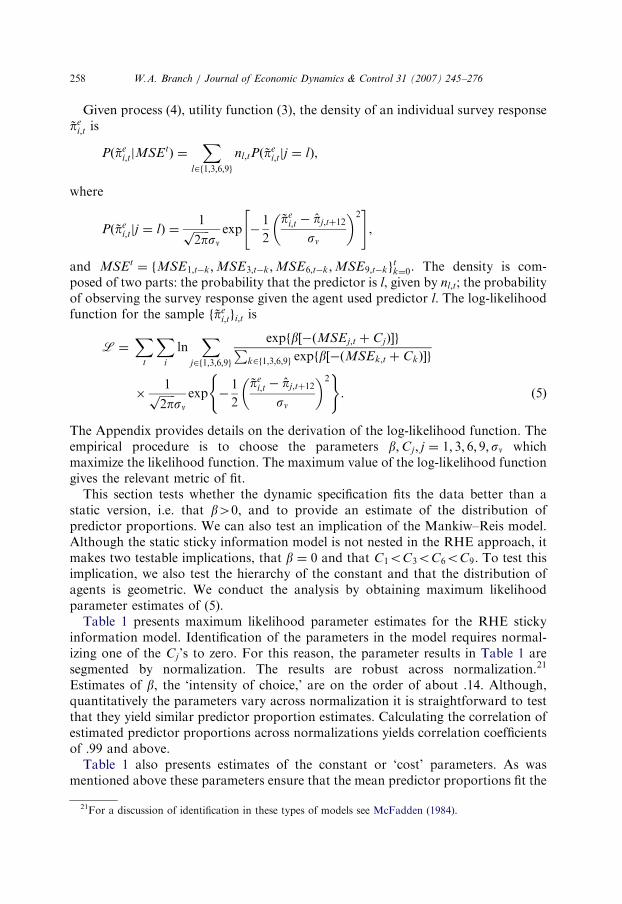
The Appendix provides details on the derivation of the log-likelihood function. Theempirical procedure is to choose the parameters b;Cj ; j ¼ 1; 3; 6; 9; sn whichmaximize the likelihood function. The maximum value of the log-likelihood functiongives the relevant metric of fit.

This section tests whether the dynamic specification fits the data better than astatic version, i.e. that b40, and to provide an estimate of the distribution ofpredictor proportions. We can also test an implication of the Mankiw–Reis model.Although the static sticky information model is not nested in the RHE approach, itmakes two testable implications, that b ¼ 0 and that C1oC3oC6oC9. To test thisimplication, we also test the hierarchy of the constant and that the distribution ofagents is geometric. We conduct the analysis by obtaining maximum likelihoodparameter estimates of (5).

Table 1 presents maximum likelihood parameter estimates for the RHE stickyinformation model. Identification of the parameters in the model requires normal-izing one of the Cj’s to zero. For this reason, the parameter results in Table 1 aresegmented by normalization. The results are robust across normalization.21

Estimates of b, the ‘intensity of choice,’ are on the order of about .14. Although,quantitatively the parameters vary across normalization it is straightforward to testthat they yield similar predictor proportion estimates. Calculating the correlation ofestimated predictor proportions across normalizations yields correlation coefficientsof :99 and above.

Table 1 also presents estimates of the constant or ‘cost’ parameters. As wasmentioned above these parameters ensure that the mean predictor proportions fit the

21For a discussion of identification in these types of models see McFadden (1984).

ARTICLE IN PRESS

Table 1

Maximum likelihood estimation results

Normalization Parameter estimates

b C1 C3 C6 C9 sn

Predictor 1 0.1439 0 �0.6718 �1.344 0.1309 6.0044

ð0:3620e� 007Þ ð0:2236e� 007Þ ð0:4486e� 007Þ ð0:1660e� 007Þ ð0:2897e� 005Þ

Predictor 3 0.1363 0.3598 0 �0.8648 0.5651 6.0037


Predictor 6 0.1418 1.3132 0.6509 0 1.4327 6.005


Predictor 9 0.1442 �0.1182 �0.809 �1.4703 0 6.0048



data best. Under each normalization the predictor updated every 6 months carriesthe lowest cost. Following the 6-month predictor the ordering is C3oC1oC9. Thisimplies that, on average, the predictors updated every 3 and 6 months are used by agreater proportion of agents than the predictors updated very frequently (j ¼ 1) andinfrequently (j ¼ 9). Although this structure is different than the static stickyinformation alternative – where the highest proportion of agents update each period– these results are intuitive. Given the low volatility in the annual inflation series, weshould expect that if agents are predisposed to not updating information everyperiod, then the 3- and 6-month predictors should be the most popular: all else equal,lower cost implies higher proportions which use that predictor.22

That we have bound the least updated predictor at 9 months – while the staticsticky information model has updating every 12 months on average – does not affectthis result. We placed the bound because predictors updated every 9 months or lessproduce forecasts too similar and create an identification problem. As mentionedabove, the empirical strategy will identify agents who update every 12 or moremonths as using the 9 month predictor. If it were possible to identify a distinct 12 (or24) month predictor the qualitative results would be identical.

The finding that the constants, or ‘costs’, lead to the 9-month predictor carryingthe highest cost is not paradoxical. In the ARED the cost acts as a threshold thatforecast errors must cross to induce agents to switch forecast methods: we interpretthese parameters also as a threshold or predisposition effect. Empirically, they ensurethat the estimated proportions fit the data best.

These results shed light on the nature of sticky information in survey data. Weproposed two alternative models of limited information flows. The first was a staticmodel with a geometric distribution of agents across models. The second is adynamic model of RHE sticky information. We tested the hypothesis H0 : b ¼ 0 andfound a log-likelihood value of �1:4619� 106, thus, in a likelihood ratio test, we

22This intuition implicitly assumes that people are inclined to update more than once a year.

ARTICLE IN PRESS


reject the null that b ¼ 0. Moreover, our estimates of the constants suggest thatagents are not distributed geometrically. These results indicate that if stickyinformation exists in survey data, it takes a dynamic form. We emphasize that theseresults exist when we restrict ourselves to the class of sticky information models. Thenext section expands the comparison to a larger class of non-nested models.However, the finding of a non-geometric distribution is a primary finding of thispaper.

There are two distinctions in the RHE sticky information from the static stickyinformation model: each predictor is updated at different rates; the proportionsacross these predictors are time-varying. The restriction that b ¼ 0 is the case wherethere is heterogeneous updating but with fixed proportions. Thus, the test of therestriction H0 : b ¼ 0 is a test of whether these two distinguishing properties arejointly significant. As will be seen below, it is the time-varying proportions that areimportant in accounting for the evolution of survey expectations.

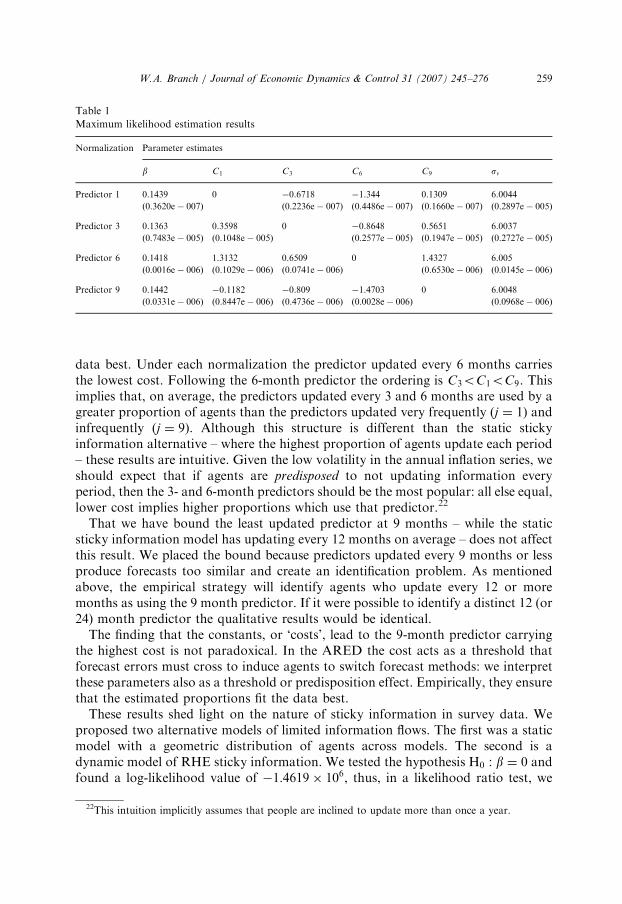
Fig. 1 plots the estimated predictor proportions. These proportions are estimatedby simulating (2) and (3) with the parameter estimates in Table 1. On average,predictors 6 and 3 are used most frequently, followed by predictors 1 and 9 in thatorder. The most striking feature of Fig. 1 is the volatility around the mean predictorproportions. Although the predictors 3 and 6 are used most often, on average, thereare times when few agents are identified with them. In fact, at times many agents

0.0

0.2

0.4

0.6

0.8

1.0

78 80 82 84 86 88 90 920.0

0.2

0.4

0.6

0.8

1.0

78 80 82 84 86 88 90 92

0.0

0.2

0.4

0.6

0.8

1.0

78 80 82 84 86 88 90 920.0

0.2

0.4

0.6

0.8

1.0

78 80 82 84 86 88 90 92

n1 n3

n6 n9

Fig. 1. Estimated proportions.

ARTICLE IN PRESS


have full-information while other periods a scant minority do. Most of the volatilityin predictor proportions occurs during the great inflation and disinflation, in linewith the hypothesis of Brock and Durlauf (2004). Greater volatility in proportionsduring periods of high economic volatility is predicted by the model. This is becauseagents are assumed to respond to the most recent squared forecast error, and it ismore likely that predictors with higher average errors will coincidentally produce thelowest error in a given period in such times.23 The figure also demonstrates how theconstants create a threshold or predisposition effect. It is only when forecast errorsrise above this threshold that the proportions of agents decrease from their meanvalues. We conclude that dynamic sticky information is consistent with the surveydata. It would be interesting for future research to investigate whether thesedynamics could be implied by an extension of Reis (2004) to a setting with structuralchange.

4. Fitting the full distribution

The results above are not evidence that the RHE sticky information model fits thesurvey data better than the Mankiw–Reis model. Because of the timing differencesbetween the two models, it is not possible to nest the Mankiw–Reis approach as atestable restriction of the RHE approach; the RHE approaches have more freeparameters. Similarly, it is also not possible to present likelihood evidence in favor oragainst RHE sticky information vis-a-vis the RHE model uncertainty of Branch(2004). It is because these models are all non-nested that we turn in this section to anon-parametric approach.

A complete model comparison should study which reduced-form models ofexpectation formation track the shifting distribution of survey responses acrosstime. A theoretical model of heterogeneous expectations suggests two channelsfor a time-varying distribution of survey expectations. The first is through thedistinct response of heterogeneous forecasting models to economic innovations.The second is through a dynamic switching between forecast models. The firstchannel is implied by both the static sticky information model and the two RHEmodels. The Mankiw–Reis approach implies a time-varying distribution becauseagents’ beliefs will adjust differently to economic shocks based on how frequentlythey update their information sets. Mankiw et al. (2003) demonstrate that a staticsticky information model, during a period such as the great disinflation, mayproduce ‘disagreement’ in the form of a multi-peaked distribution with skewnesswhich varies over time. The RHE approaches also may yield divergent expectationsbecause each heterogeneous forecasting model may respond distinctly to economicshocks. The RHE models are also consistent with the second channel: agentsdynamically select their forecasting model based on past forecast success. Thus, the

23One concern may be that the higher volatility, observed at the beginning of the survey sample is

because of transient behavior. As detailed above, we used a pre-sample initialization period to eliminate

transient dynamics.

ARTICLE IN PRESS


dynamic predictor selection mechanism, at its very core, is a theory of time-varyingdistributions.

Our interest is not to compare the fit to the entire sample of survey data, but howeach model fits the survey data in each period. The hypotheses are: the evolution ofthe distribution of survey responses results from the dynamics of the economy whenexpectations are formed according to the static sticky information model; the changein the distribution of survey responses is because agents adapt their predictor choiceand so the degree of heterogeneity is time-varying.

4.1. Non-parametric estimation of density functions

Our methodology is non-parametric estimation of the density functions and thehistogram of the survey data. We make sample draws from the estimateddistribution functions of all three alternative approaches. Taking the histogram ofthe survey data as the density function of the true model, we construct non-parametric estimates of the model density functions and compare their fit with thehistogram from the actual data set. This allows a test for whether any of the modelsare the same as the true economic model of expectation formation. We also provide ameasure of ‘closeness’ between these models and the data. We follow White (1994)and conclude that the model which yields the smallest measure between densities isalso the model most consistent with the data.

To estimate the density functions we make 465 draws from the distribution definedby each model in each time period.24 For the RHE sticky information model (2), (3)and (4) defines a density function given the estimated parameters in Table 1. Fromthis estimated density function we generate a sample of predicted survey responses.Given an assumption on the information flow parameter l, it is also possible to makerandom draws from the static sticky information model’s distribution. We followMankiw et al. (2003) in fixing l ¼ :10. Along these lines, we draw from the samedistribution estimated in Branch (2004).

The first question to address is whether these three models of expectationformation have distinct implications about the economy. To this end, Fig. 2 plotsthe mean responses of these draws from the estimated density functions. Thefigure makes it clear that each model yields quantitatively different predictionsabout survey responses. For instance, the static sticky information model adjustsslowly to the great disinflation as it takes time for information to disseminatethrough all agents’ information sets. The RHE model uncertainty respondsto changes in the economic environment more quickly as agents adjust to pastforecast errors.

We first present hypothesis test results. Following the framework in Pagan andUllah (1999), denote dðpeÞ; f ðpeÞ; gðpeÞ; hðpeÞ as the true densities of the Mankiw–Reissticky information model, the RHE sticky information model, the RHEmodel uncertainty case and the survey data, respectively. The Appendix detailsconstruction of the estimates d; f ; g; h and hypothesis tests. We are interested in the

24A sample size of 465 is approximately the mean size each period of the Michigan survey.

ARTICLE IN PRESS

-4

0

4

8

12

16

80 82 84 86 88 90 92

Mean Forecast: static sticky info.Mean Forecast: RHE-model uncertaintyMean Forecast: RHE-sticky info.

Fig. 2. Plot of mean forecasts from various models.


following hypotheses,

H0 : dðpeÞ ¼ hðpeÞ,

H0 : f ðpeÞ ¼ hðpeÞ,

H0 : gðpeÞ ¼ hðpeÞ.

We report two test statistics T ;T1 of these hypotheses which are distributed standardnormal.

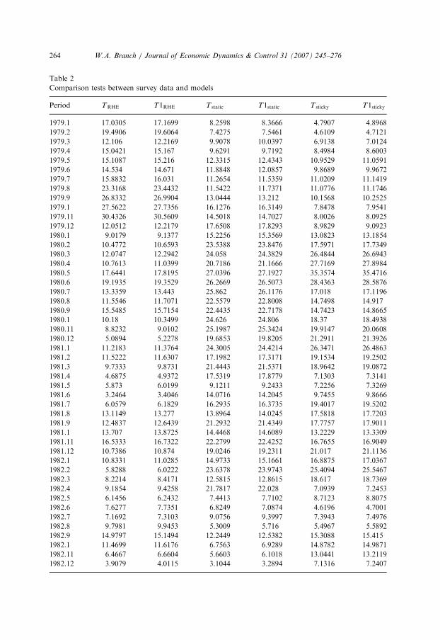
Table 2 reports the results of the hypothesis tests. The tests are computed monthlybetween 1979.1 and 1982.12. We report results for this period because it isemphasized in Mankiw et al. (2003) who hypothesize that sticky information shouldbe most evident during the great disinflation. In each case, we reject the nullhypothesis at the .01 significance level.25 This suggests that none of the modelalternatives are identical to the actual survey data generating process.

That none of our alternative expectation formation models match up statisticallywith the survey data is not surprising. We now turn to other measures of fit besideshypothesis testing. We address this issue by constructing a measure of closenessbetween the estimated densities. The measure adopted here is the Kullback–Leiblerdistance measure of White (1994).26 If the Kullback–Leibler measure equals a

25We note that estimates of whether the models are the same as the actual data over the whole sample

period are also rejected.26Details are in the Appendix.

ARTICLE IN PRESS

Table 2

Comparison tests between survey data and models

Period TRHE T1RHE T static T1static T sticky T1sticky

1979.1 17.0305 17.1699 8.2598 8.3666 4.7907 4.8968

1979.2 19.4906 19.6064 7.4275 7.5461 4.6109 4.7121

1979.3 12.106 12.2169 9.9078 10.0397 6.9138 7.0124

1979.4 15.0421 15.167 9.6291 9.7192 8.4984 8.6003

1979.5 15.1087 15.216 12.3315 12.4343 10.9529 11.0591

1979.6 14.534 14.671 11.8848 12.0857 9.8689 9.9672

1979.7 15.8832 16.031 11.2654 11.5359 11.0209 11.1419

1979.8 23.3168 23.4432 11.5422 11.7371 11.0776 11.1746

1979.9 26.8332 26.9904 13.0444 13.212 10.1568 10.2525

1979.1 27.5622 27.7356 16.1276 16.3149 7.8478 7.9541

1979.11 30.4326 30.5609 14.5018 14.7027 8.0026 8.0925

1979.12 12.0512 12.2179 17.6508 17.8293 8.9829 9.0923

1980.1 9.0179 9.1377 15.2256 15.3569 13.0823 13.1854

1980.2 10.4772 10.6593 23.5388 23.8476 17.5971 17.7349

1980.3 12.0747 12.2942 24.058 24.3829 26.4844 26.6943

1980.4 10.7613 11.0399 20.7186 21.1666 27.7169 27.8984

1980.5 17.6441 17.8195 27.0396 27.1927 35.3574 35.4716

1980.6 19.1935 19.3529 26.2669 26.5073 28.4363 28.5876

1980.7 13.3359 13.443 25.862 26.1176 17.018 17.1196

1980.8 11.5546 11.7071 22.5579 22.8008 14.7498 14.917

1980.9 15.5485 15.7154 22.4435 22.7178 14.7423 14.8665

1980.1 10.18 10.3499 24.626 24.806 18.37 18.4938

1980.11 8.8232 9.0102 25.1987 25.3424 19.9147 20.0608

1980.12 5.0894 5.2278 19.6853 19.8205 21.2911 21.3926

1981.1 11.2183 11.3764 24.3005 24.4214 26.3471 26.4863

1981.2 11.5222 11.6307 17.1982 17.3171 19.1534 19.2502

1981.3 9.7333 9.8731 21.4443 21.5371 18.9642 19.0872

1981.4 4.6875 4.9372 17.5319 17.8779 7.1303 7.3141

1981.5 5.873 6.0199 9.1211 9.2433 7.2256 7.3269

1981.6 3.2464 3.4046 14.0716 14.2045 9.7455 9.8666

1981.7 6.0579 6.1829 16.2935 16.3735 19.4017 19.5202

1981.8 13.1149 13.277 13.8964 14.0245 17.5818 17.7203

1981.9 12.4837 12.6439 21.2932 21.4349 17.7757 17.9011

1981.1 13.707 13.8725 14.4468 14.6089 13.2229 13.3309

1981.11 16.5333 16.7322 22.2799 22.4252 16.7655 16.9049

1981.12 10.7386 10.874 19.0246 19.2311 21.017 21.1136

1982.1 10.8331 11.0285 14.9733 15.1661 16.8875 17.0367

1982.2 5.8288 6.0222 23.6378 23.9743 25.4094 25.5467

1982.3 8.2214 8.4171 12.5815 12.8615 18.617 18.7369

1982.4 9.1854 9.4258 21.7817 22.028 7.0939 7.2453

1982.5 6.1456 6.2432 7.4413 7.7102 8.7123 8.8075

1982.6 7.6277 7.7351 6.8249 7.0874 4.6196 4.7001

1982.7 7.1692 7.3103 9.0756 9.3997 7.3943 7.4976

1982.8 9.7981 9.9453 5.3009 5.716 5.4967 5.5892

1982.9 14.9797 15.1494 12.2449 12.5382 15.3088 15.415

1982.1 11.4699 11.6176 6.7563 6.9289 14.8782 14.9871

1982.11 6.4667 6.6604 5.6603 6.1018 13.0441 13.2119

1982.12 3.9079 4.0115 3.1044 3.2894 7.1316 7.2407


ARTICLE IN PRESS


positive number then the area between two density functions is positive. We say thatthe model with the lowest distance measure is the model most consistent with howsurvey responses are formed. Using the Kullback–Leibler preferred model is anappealing model selection criteria because there is a complete axiomatic foundationsupporting it (see Shore and Johnson, 1980; Csiszar, 1991).

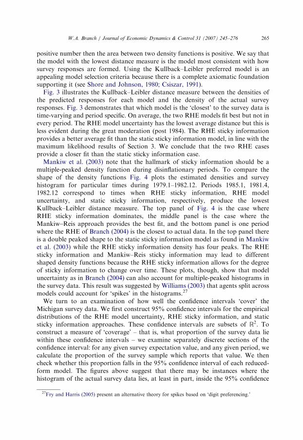
Fig. 3 illustrates the Kullback–Leibler distance measure between the densities ofthe predicted responses for each model and the density of the actual surveyresponses. Fig. 3 demonstrates that which model is the ‘closest’ to the survey data istime-varying and period specific. On average, the two RHE models fit best but not inevery period. The RHE model uncertainty has the lowest average distance but this isless evident during the great moderation (post 1984). The RHE sticky informationprovides a better average fit than the static sticky information model, in line with themaximum likelihood results of Section 3. We conclude that the two RHE casesprovide a closer fit than the static sticky information case.

Mankiw et al. (2003) note that the hallmark of sticky information should be amultiple-peaked density function during disinflationary periods. To compare theshape of the density functions Fig. 4 plots the estimated densities and surveyhistogram for particular times during 1979.1–1982.12. Periods 1985.1, 1981.4,1982.12 correspond to times when RHE sticky information, RHE modeluncertainty, and static sticky information, respectively, produce the lowestKullback–Leibler distance measure. The top panel of Fig. 4 is the case whereRHE sticky information dominates, the middle panel is the case where theMankiw–Reis approach provides the best fit, and the bottom panel is one periodwhere the RHE of Branch (2004) is the closest to actual data. In the top panel thereis a double peaked shape to the static sticky information model as found in Mankiwet al. (2003) while the RHE sticky information density has four peaks. The RHEsticky information and Mankiw–Reis sticky information may lead to differentshaped density functions because the RHE sticky information allows for the degreeof sticky information to change over time. These plots, though, show that modeluncertainty as in Branch (2004) can also account for multiple-peaked histograms inthe survey data. This result was suggested by Williams (2003) that agents split acrossmodels could account for ‘spikes’ in the histograms.27

We turn to an examination of how well the confidence intervals ‘cover’ theMichigan survey data. We first construct 95% confidence intervals for the empiricaldistributions of the RHE model uncertainty, RHE sticky information, and staticsticky information approaches. These confidence intervals are subsets of R2. Toconstruct a measure of ‘coverage’ – that is, what proportion of the survey data liewithin these confidence intervals – we examine separately discrete sections of theconfidence interval: for any given survey expectation value, and any given period, wecalculate the proportion of the survey sample which reports that value. We thencheck whether this proportion falls in the 95% confidence interval of each reduced-form model. The figures above suggest that there may be instances where thehistogram of the actual survey data lies, at least in part, inside the 95% confidence

27Fry and Harris (2005) present an alternative theory for spikes based on ‘digit preferencing.’

ARTICLE IN PRESS

0.0

0.1

0.2

0.3

0.4

0.5

0.6

80 82 84 86 88 90 92

0.0

0.1

0.2

0.3

0.4

0.5

0.6

80 82 84 86 88 90 92

0.0

0.1

0.2

0.3

0.4

0.5

0.6

80 82 84 86 88 90 92

RHE Case

Static Sticky Information Case

RHE Sticky Information Case

Fig. 3. Kullback–Leibler distance measures for various models.


ARTICLE IN PRESS

-5 0 5 10 15 200

0.35

-5 0 5 10 15 200

0.4

-5 0 5 10 15 200

RHE model uncertaintysurvey datastatic sticky informationRHE sticky information

0.3

0.25

0.2

0.15

0.1

0.05

0.45

0.35

0.3

0.25

0.2

0.15

0.1

0.05

0.45

0.4

0.35

0.3

0.25

0.2

0.15

0.1

0.05



Fig. 4. Comparisons of histograms. Top panel (1985.1) is where RHE sticky information provides best fit.

Middle panel (1982.12) is where static sticky information provides best fit. Bottom panel (1981.4) is where

RHE model uncertainty fists best.


ARTICLE IN PRESS

00

10

20

30

40

50

60

70

RHE model uncertainty

Static sticky information

0.05 0.1 0.15 0.2 0.25 0.3 0.35 0.4 0.45 0.5

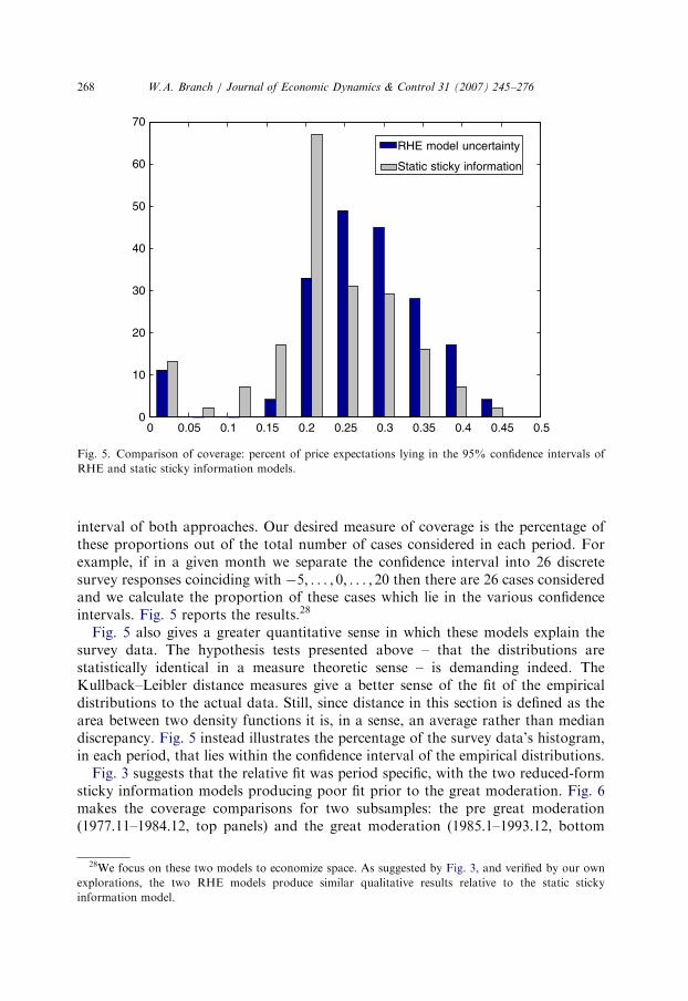
Fig. 5. Comparison of coverage: percent of price expectations lying in the 95% confidence intervals of

RHE and static sticky information models.


interval of both approaches. Our desired measure of coverage is the percentage ofthese proportions out of the total number of cases considered in each period. Forexample, if in a given month we separate the confidence interval into 26 discretesurvey responses coinciding with �5; . . . ; 0; . . . ; 20 then there are 26 cases consideredand we calculate the proportion of these cases which lie in the various confidenceintervals. Fig. 5 reports the results.28

Fig. 5 also gives a greater quantitative sense in which these models explain thesurvey data. The hypothesis tests presented above – that the distributions arestatistically identical in a measure theoretic sense – is demanding indeed. TheKullback–Leibler distance measures give a better sense of the fit of the empiricaldistributions to the actual data. Still, since distance in this section is defined as thearea between two density functions it is, in a sense, an average rather than mediandiscrepancy. Fig. 5 instead illustrates the percentage of the survey data’s histogram,in each period, that lies within the confidence interval of the empirical distributions.

Fig. 3 suggests that the relative fit was period specific, with the two reduced-formsticky information models producing poor fit prior to the great moderation. Fig. 6makes the coverage comparisons for two subsamples: the pre great moderation(1977.11–1984.12, top panels) and the great moderation (1985.1–1993.12, bottom

28We focus on these two models to economize space. As suggested by Fig. 3, and verified by our own

explorations, the two RHE models produce similar qualitative results relative to the static sticky

information model.

ARTICLE IN PRESS

00

2

4

6

8

10

12

14

16

18

201977.11-1984.12

0

2

4

6

8

10

12

14

16

18

201977.11-1984.12

0

5

10

15

20

0

5

10

15

20

25

30

351985.01-1993.12

RHE model uncertaintyStatic sticky info.

35

30

25

0.05 0.1 0.15 0.50.450.40.350.30.250.2

0.50.450.40.350.30.250.20.150.10.450.40.350.30.250.20.150.10.05

0.50.450.40.350.30.250.20.150.10.05

1985.01-1993.12

RHE model uncertaintyRHE sticky info.

RHE model uncertaintyStatic sticky info.

RHE model uncertaintyRHE sticky info.

Fig. 6. Comparison of coverage. Left panels for the pre-Great Moderation period, right panels for the

Great Moderation. Upper panels compare RHE model uncertainty and static sticky information. Lower

panels compare RHE model uncertainty and RHE sticky information.


panels). The left panels compare RHE model uncertainty to static sticky informationand the right graphs compare the two RHE models. As a metric of fit we say that amodel provides better coverage if the number of periods in which the coveragepercentage is greater than .25 is higher than the alternative. Using this measure, Fig.6 suggests that the two models with time-varying distribution have greater coveragethan the static sticky information alternative. This is particularly true during thegreat moderation. Fig. 6 also suggests the RHE sticky information has greatercoverage than the RHE model uncertainty during the great moderation.

ARTICLE IN PRESS


These findings suggest an interpretation along the following lines: during periodsof economic volatility, like the 1970s, the RHE model uncertainty alternativefits best; during the great moderation of the 1980s and 1990s the RHE stickyinformation model provides a closer fit.

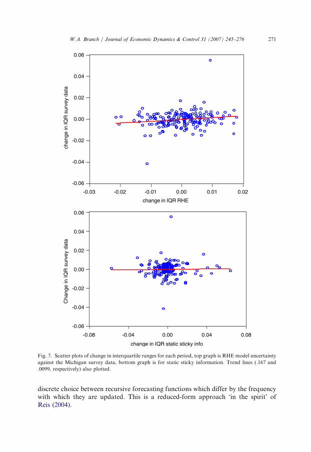
Ultimately, this paper argues, through parametric and non-parametric evidence, infavor of those models that are able to capture the evolution across time of thedistribution of survey data. Fig. 7, top panel, provides further evidence on how wellthe RHE models capture the time-varying dispersion of the survey responses. Fig. 7reports the interquartile range (IQR) of the estimated density functions. The IQR isthe computed difference between the 75th and the 25th percentiles of the estimateddensity functions, for each period of the sample. Tracking the IQR overtime gives anestimate of how the dispersion of the data changes over time. It has the advantageover Kullback–Leibler in that it ignores the tails of the distribution. The top panel ofFig. 7 scatters changes in the IQR for the RHE model against changes in the IQR forthe survey data, and the bottom graph does similarly for the static sticky informationmodel.29 Each figure also plots the trend line. The slope of the trend in the top andbottom panels are .167 and .0099, respectively.

In Fig. 7, top panel, there is an upward trend suggesting that as the survey databecomes more disperse over time, then the RHE model uncertainty approachpredicts a greater dispersion of the survey data as well. In the bottom panel, thetrend line is increasing slightly, but the slope is not statistically different from zero.The positive correlation between the RHE model’s IQR and the Michigan survey’sIQR demonstrates that the model uncertainty approach can explain, in part, thetime-varying dispersion of the survey data. The main difference in the IQRs for theRHE and static sticky information approach is that the static sticky informationapproach is more likely to predict little or wide dispersion. This is a feature of theMankiw–Reis structure of overlapping information updating: in periods of relativeeconomic stability the degree of heterogeneity is small and as the economy switchesto a period of instability the dispersion will be higher.

5. Conclusion

This paper examined three reduced-form models of heterogeneous expectations.This paper achieved two objectives: first, a characterization of sticky information insurvey data; second, an examination of how well each model fits the full distributionof survey responses. We compared two models of sticky information againstthe RHE model uncertainty approach of Branch (2004). Our first model ofsticky information was an application of the novel approach in Mankiw andReis (2002). Our second model, was an extension of Mankiw and Reis (2002) tothe framework of Brock and Hommes (1997) where we assume agents make a

29Plotting the level of IQR produces similar results as Fig. 7. Also, the plot for changes in IQR for the

RHE sticky information model produces a similar, though less steep, trend as the RHE model uncertainty

case.

ARTICLE IN PRESS

change in IQR RHE

chan

ge in

IQR

sur

vey

data

change in IQR static sticky info

Cha

nge

in IQ

R s

urve

y da

ta

0.06

0.04

0.02

0.00

-0.02

-0.04

-0.06

-0.03 -0.02 -0.01 0.00 0.01 0.02

0.080.040.00-0.04-0.08

0.06

0.04

0.02

0.00

-0.02

-0.04

-0.06

Fig. 7. Scatter plots of change in interquartile ranges for each period, top graph is RHE model uncertainty

against the Michigan survey data, bottom graph is for static sticky information. Trend lines (.167 and

.0099, respectively) also plotted.


discrete choice between recursive forecasting functions which differ by the frequencywith which they are updated. This is a reduced-form approach ‘in the spirit’ ofReis (2004).

ARTICLE IN PRESS


We first characterized limited information flows in the survey data by restrictingagents to a particular class of sticky information models. In the paper’s main results,we show that a sticky information model with a time-varying distribution structureprovides a better fit than the static approach of Mankiw and Reis (2002). We providemaximum likelihood evidence that, on average, the highest proportion of agents inthe Michigan survey update their information sets every 3–6 months. A lowerproportion of agents update their expectations every period and few agents updatetheir expectations at periods of 9 months or more. We also provide evidence, likeBranch (2004), that these proportions vary over time.

We also presented a test of whether any of the three expectation formation modelsimply a density function identical to the density of the true model. We reject thehypothesis that any of these models are identical to the data generating process.Instead we provide non-parametric measures of fit. Non-parametric evidencesuggests that the two rationally heterogeneous expectations models provide a betterfit than the static sticky information model. We construct estimates of the densityfunctions for each model and compare them to the histogram of the actual surveydata. However, this result holds, on average, and there are periods, particularlyduring the late 1980s and early 1990s, in which static sticky information provides thebest fit.

These results are significant. There is considerable interest in the appliedliterature on the effects of model uncertainty and sticky information. Thispaper suggests that both may be elements of the data. Most significantly, thedistribution of heterogeneity is non-geometric and time-varying. The modelspresented here, though, do not allow for sticky information across competingmodels of the economy. Future research should address structural explanations ofthese findings.

Acknowledgments

This paper has benefited enormously from comments and suggestions by theEditor, Peter Ireland, two anonymous referees, Bruce McGough, Fabio Milani, andKen Small.

Appendix A. Log-likelihood function derivation

Recall, that the actual observed survey response is given by

~pei;t ¼ pj;tþ12 þ ni;t, (6)

where pj;tþ12 2 fp1;tþ12; p3;tþ12; p6;tþ12; p9;tþ12g. The probability of using the jthpredictor was given by the theoretical model as a MNL,

PrðjjUj;tÞ ¼ nj;t ¼expfb½�ðMSEj;t þ CjÞ�gP

k2f1;3;6;9g expfb½�ðMSEk;t þ CkÞ�g.

ARTICLE IN PRESS


Since vi;t is distributed normally, the density of ~pei;t is

Pð ~pei;tjMSEtÞ ¼

Xk2f1;3;6;9g

nk;tPð ~pei;tjj ¼ kÞ,

where MSEt ¼ fMSEj;tgj2f1;3;6;9g and

Pð ~pei;tjj ¼ kÞ ¼

1ffiffiffiffiffiffi2pp

snexp �

1

2

~pei;t � pj;tþ12

sv

� �2( )

.

Since the sample changes each period, the probability of observing the sample isgiven by the following density function:

Pð ~pei;t; i ¼ 1; . . . ;N; t ¼ 1; . . . ;T jMSEt;HtðptÞ; t ¼ 1; . . . ;TÞ

¼Y

t

Yi

Pð ~pei;tjMSEtÞ

¼Y

t

Yi

Xk2f1;3;6;9g

nk;tPð ~pei;tjj ¼ kÞ

( ).

Taking logs leads to form (5).

Appendix B. Non-parametric density estimation

We discuss the details of the non-parametric density estimation in Section 3.3. Ourapproach uses the Rosenblatt–Parzen kernel estimator as detailed in Pagan andUllah (1999). This approach computes an empirical density function. Essentially itreplaces a histogram, which computes the number of observations in a givenwindow-width, with a probability density function which assigns a probability massto a given window-width. Thus, the kernel estimator is

f ðxÞ ¼1

nh

Xn

i¼1

Kxi � x

h

� �,

where f is the estimator of f, the true density, fxigni¼1 is the sequence of observed

values, and h is the window-width. The function K is the kernel function which isusually chosen to be a well-known probability density function. Following Paganand Ullah (1999) we choose K to be the pdf of a standard normal. The remainingissue is the selection of h. Clearly the estimator is sensitive to the choice of h. We notethat Figs. 4–6 are illustrative and not a test of the validity of the estimate densityfunctions. The density hypothesis testing are robust to choices of h. Pagan and Ullahnote that a popular choice of h is one that minimizes the integrated mean squarederror, which is essentially a measure of both the bias and variance of the estimates.The recommendation of this approach is to set h ¼ n�:2 where n is the number ofobservations in the sample.

ARTICLE IN PRESS


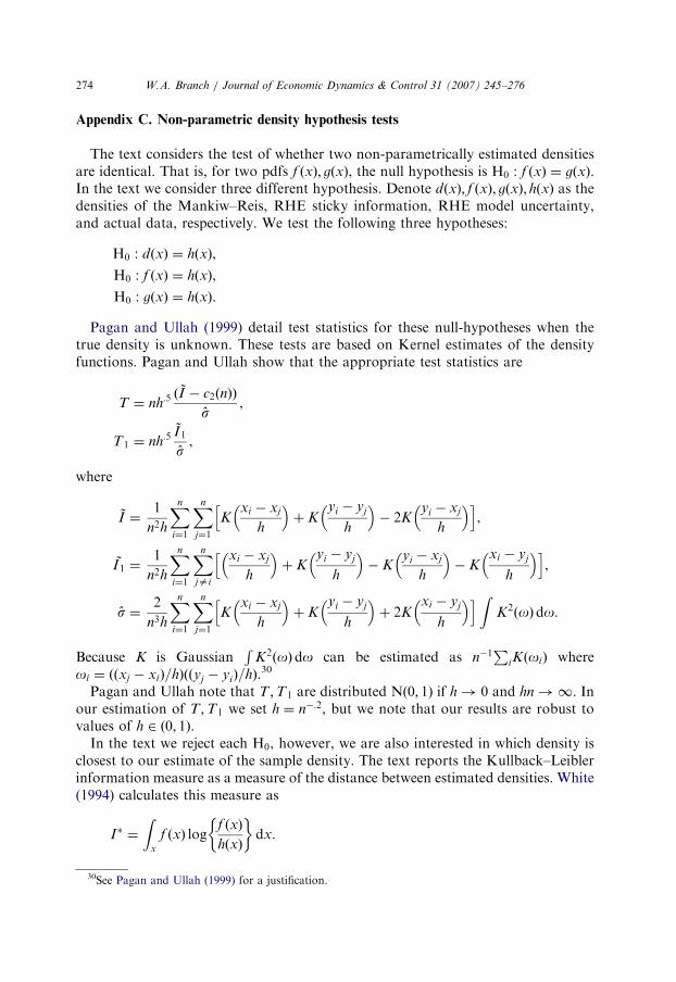
Appendix C. Non-parametric density hypothesis tests

The text considers the test of whether two non-parametrically estimated densitiesare identical. That is, for two pdfs f ðxÞ; gðxÞ, the null hypothesis is H0 : f ðxÞ ¼ gðxÞ.In the text we consider three different hypothesis. Denote dðxÞ; f ðxÞ; gðxÞ; hðxÞ as thedensities of the Mankiw–Reis, RHE sticky information, RHE model uncertainty,and actual data, respectively. We test the following three hypotheses:

H0 : dðxÞ ¼ hðxÞ,

H0 : f ðxÞ ¼ hðxÞ,

H0 : gðxÞ ¼ hðxÞ.

Pagan and Ullah (1999) detail test statistics for these null-hypotheses when thetrue density is unknown. These tests are based on Kernel estimates of the densityfunctions. Pagan and Ullah show that the appropriate test statistics are

T ¼ nh:5ð ~I � c2ðnÞÞ

s,

T1 ¼ nh:5~I1s,

where

~I ¼1

n2h

Xn

i¼1

Xn

j¼1

Kxi � xj

h

� �þ K

yi � yj

h

� �� 2K

yi � xj

h

� �h i,

~I1 ¼1

n2h

Xn

i¼1

Xn

jai

xi � xj

h

� �þ K

yi � yj

h

� �� K

yi � xj

h

� �� K

xi � yj

h

� �h i,

s ¼2

n3h

Xn

i¼1

Xn

j¼1

Kxi � xj

h

� �þ K

yi � yj

h

� �þ 2K

xi � yj

h

� �h i ZK2ðoÞdo.

Because K is GaussianR

K2ðoÞdo can be estimated as n�1P

iKðoiÞ whereoi ¼ ððxj � xiÞ=hÞððyj � yiÞ=hÞ.30

Pagan and Ullah note that T ;T1 are distributed Nð0; 1Þ if h! 0 and hn!1. Inour estimation of T ;T1 we set h ¼ n�:2, but we note that our results are robust tovalues of h 2 ð0; 1Þ.

In the text we reject each H0, however, we are also interested in which density isclosest to our estimate of the sample density. The text reports the Kullback–Leiblerinformation measure as a measure of the distance between estimated densities. White(1994) calculates this measure as

I� ¼

Zx

f ðxÞ logf ðxÞ

hðxÞ

� �dx.

30See Pagan and Ullah (1999) for a justification.

ARTICLE IN PRESS


The measure I� approximates distance in the sense that if f ðxÞ ¼ hðxÞ in theappropriate sense, then I� ¼ 0. Thus, I�a0 iff f ðxÞahðxÞ for some x. We use ournon-parametrically estimated density functions to compute this measure.

References

Aadland, D., 2004. Cattle cycles, heterogeneous expectations, and the age distribution of capital. Journal

of Economic Dynamics and Control 28(10), 1977–2002.

Baak, S.J., 1999. Tests for bounded rationality with a linear dynamic model distorted by heterogeneous

expectations. Journal of Economic Dynamics and Control 23, 1517–1543.

Ball, L., Mankiw, N.G., Reis, R., 2005. Monetary policy for inattentive economies. Journal of Monetary

Economics 52, 4.

Branch, W.A., 2004. The theory of rationally heterogeneous expectations: evidence from survey data on

inflation expectations. Economic Journal 114, 497.

Branch, W.A., Evans, G.W., 2005. A simple recursive forecasting model. Economics Letters, forthcoming.

Branch, W.A., Carlson, J., Evans, G.W., McGough, B., 2004. Monetary Policy, Endogenous Inattention,

and the Inflation-Output Variance Tradeoff, Mimeo.

Brock, W.A., Durlauf, S.N., 2004. Macroeconomics and Model Uncertainty, Mimeo.

Brock, W.A., Hommes, C.H., 1997. A rational route to randomness. Econometrica 65, 1059–1160.

Brock, W.A., Hommes, C.H., Wagener, F.O.O., 2005. Evolutionary dynamics in markets with many

trader types. Journal of Mathematical Economics 41(1–2), 7–42.

Bryan, M.F., Venkatu, G., 2001a. The demographics of inflation opinion surveys. Economic

Commentary, Federal Reserve Bank of Cleveland.

Bryan, M.F., Venkatu, G., 2001b. The curiously different inflation perspectives of men and women.

Economic Commentary, Federal Reserve Bank of Cleveland.

Calvo, G., 1983. Staggered prices in a utility-maximizing framework. Journal of Monetary Economics 12,

393–398.

Carroll, C.D., 2003. The epidemiology of macroeconomic expectations. Quarterly Journal of Economics

118, 1.

Chavas, J.-P., 2000. On information and market dynamics: the case of the U.S. beef market. Journal of

Economic Dynamics and Control 24, 833–853.

Croushore, D., Stark, T., 2003. A real-time data set for macroeconomists: does the data vintage matter?

Review of Economics and Statistics 85, 605–617.

Csiszar, I., 1991. Why least squares and maximum entropy? An axiomatic approach to inference for linear

inverse problems. Annals of Statistics 19 (4), 2032–2066.

Evans, G.W., Honkapohja, S., 2001. Learning and Expectations in Macroeconomics. Princeton University

Press, Princeton, NJ.

Fry, T.R.L., Harris, M.N., 2005. The dogit ordered generalized extreme value model. Australian and New

Zealand Journal of Statistics, forthcoming.

Heemeijer, P., Hommes, C.H., Sonnemans, J., Tuinstra, J., 2004. Forming Price Expectations in Positive

and Negative Feedback Systems, Mimeo.

Hommes, C.H., Sonnemans, J., Tuinstra, J., van de Velden, H., 2005. A strategy experiment in dynamic

asset pricing. Review of Financial Studies 18, 955–980.

Mankiw, N.G., Reis, R., 2002. Sticky information versus sticky prices: a proposal to replace the New

Keynesian Phillips curve. Quarterly Journal of Economics 117 (4), 1295–1328.

Mankiw, N.G., Reis, R., Wolfers, J., 2003. Disagreement about inflation expectations. In: Gertler, M.,

Rogoff, K. (Eds.). NBER Macroeconomics Annual 2003.

Manski, C.F., McFadden, D., 1981. Structural Analysis of Discrete Data with Econometric Applications.

MIT Press, Cambridge, MA (Trilligator, Elsevier).

McFadden, D., 1984. Econometric analysis of qualitative response models. Handbook of Econometrics,

vol. II. In: Griliches, Z., Intrilligator, M.D. (Eds.). Elsevier, Amsterdam.

Pagan, A., Ullah, A., 1999. Nonparametric Econometrics. Cambridge University Press, Cambridge.

ARTICLE IN PRESS


Pesaran, M.H., Timmermann, A., 1995. Predictability of stock returns: robustness and economic

significance. The Journal of Finance 50 (4), 1201–1228.

Reis, R., 2004. Inattentive Producers, Mimeo.

Shore, J.E., Johnson, R.W., 1980. Axiomatic derivation of the principle of maximum entropy and the

principle of minimum-cross entropy. IEEE Transactions on Information Theory 26, 26–37.

Sims, C.A., 2003. Implications of rational inattention. Journal of Monetary Economics 50 (3), 665–690.

Sims, C.A., Zha, T., 2005. Were there regime switches in U.S. monetary policy? American Economic

Review, forthcoming.

Souleles, N.S., 2004. Consumer sentiment: its rationality and usefulness in forecasting expenditure –

evidence from the Michigan micro data. Journal of Money, Credit, and Banking 36(1), 39–72.

Stock, J.H., Watson, M.W., 1996. Evidence on structural instability in macroeconomic time series

relations. Journal of Business and Economic Statistics 14 (1), 11–30.

White, H., 1994. Estimation, Inference and Specification Analysis. Cambridge University Press,

Cambridge.

Williams, J.C., 2003. Discussion of ‘Disagreement about Inflation Expectations’. In: Gertler, M., Rogoff,

K. (Eds.). NBER Macroeconomics Annual 2003.

Woodford, M., 2003. Interest and Prices: Foundations of a Theory of Monetary Policy. Princeton

University Press, Princeton, NJ.

Sticky information and model uncertainty in survey …wbranch/Templates/stickyinfojedcpub.pdf ·...

Documents

Transcript of Sticky information and model uncertainty in survey …wbranch/Templates/stickyinfojedcpub.pdf ·...