University of Tennessee at Chattanooga

Steady State and Step Response

By: Alex Bedley

Engineering 3280L

Buff

(Alexander Hudson, Ashley Poe)

February 1, 2013

Alex Bedley February 1, 2013 2

Introduction

In the past two experiments, we were conducting experiments to obtain steady state

operating curves and step response curves with respect to certain motor input

percentages. To begin the experiments for the steady state operating curve (SSOC), trial

and error is needed to approximate the input percentage, in order to have the proper

output for each particular range (low, middle, and high). Once the desired input and

output have been figured, a graph was generated to determine the SSOC; this curve will

help to approximate an output value given at any specific input value within the desired

range.

The SSOC can help with the next lab, the objective of the second experiment is to

determine the system steady state gain, time constant, and dead time for the flow system

with a step response using a variety of different step sizes and input values.

Following the introduction, the background and the theory will be discussed in order to

provide a further detailed understanding of the lab experiment and setup process. After

the background and the theory, the operating procedure is explained in order to run the

experiment and understand the included operating variables. Results and discussion then

follow and state the values gathered in the lab in tabular and graphical form, emphasize

and the importance of the values gathered. Finally, the conclusion and recommendations

will give an overview of the results and the possible ways to improve the experiment.

Alex Bedley February 1, 2013 3

Background and Theory

The filter wash flow control system is operated via the internet. The flow system is

accessed by a link to weblab.utc.edu which can be found on the ENGR3280L

homepage. The system allows for different input percentages to be applied. These

different inputs proved specific flow rate outputs. The system inputs, the valve

positions (open or closed), and experimental time duration can be varied during the

experiment by the user.

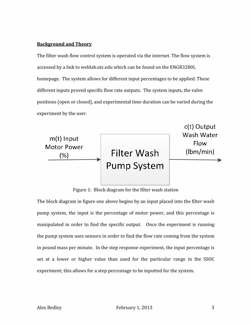
Figure 1: Block diagram for the filter wash station

The block diagram in figure one above begins by an input placed into the filter wash

pump system, the input is the percentage of motor power, and this percentage is

manipulated in order to find the specific output. Once the experiment is running

the pump system uses sensors in order to find the flow rate coming from the system

in pound mass per minute. In the step response experiment, the input percentage is

set at a lower or higher value than used for the particular range in the SSOC

experiment; this allows for a step percentage to be inputted for the system.

Alex Bedley February 1, 2013 4

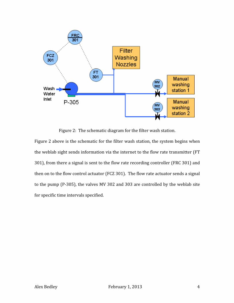
Figure 2: The schematic diagram for the filter wash station.

Figure 2 above is the schematic for the filter wash station, the system begins when

the weblab sight sends information via the internet to the flow rate transmitter (FT

301), from there a signal is sent to the flow rate recording controller (FRC 301) and

then on to the flow control actuator (FCZ 301). The flow rate actuator sends a signal

to the pump (P-305), the valves MV 302 and 303 are controlled by the weblab site

for specific time intervals specified.

Alex Bedley February 1, 2013 5

Procedure

Both experiments begin with a screen that will control the input percentage, total

time for the experiment, and the time for the valves to be closed or open. Our

system requires outputs in the range of 19-31 lbm/min with both valves closed for

the entire experimental time duration.

To begin the steady state operating experiment, a basic value needs to be guessed to

receive an output for the system. Trial and error is needed to pin point the input for

our particular output, this will take several iterations. Once the output is reached

for several values throughout the desired range, the input and output can be used to

predict a steady state operation curve. The curve predicts output given an input

multiplied by an operation constant.

The step response experiment has a place to input the beginning input percentage

and an added step value on the screen. For the step response experiment, the step

values can be either positive or negative, in order to get a step up or step down

output vs. time. The step response uses the final input that falls between the

individual ranges; the input used in the SSOC experiment will become the final value

after the step is performed. A lower or higher value is placed in the initial input on

the left side of the screen, with both valves closed and a step value must be inputted

into the right side of the screen to allow for calculations to be produced after the

experiments.

The step value must be negative for a step down function and positive for a step up.

Also inputted on the main screen of the step response is the time for the step to

Alex Bedley February 1, 2013 6

occur and total time for the experiment; the experiment worked well when the total

experiment time was around 40 seconds with a step at 20 seconds, this time frame

allowed the system to reach steady state before and after the step. At the bottom of

the screen, both valves need to be closed for the entire experiment. Once the

experiment has run the entire time set, the values from the sensor can be exported

to Excel.

Alex Bedley February 1, 2013 7

Results

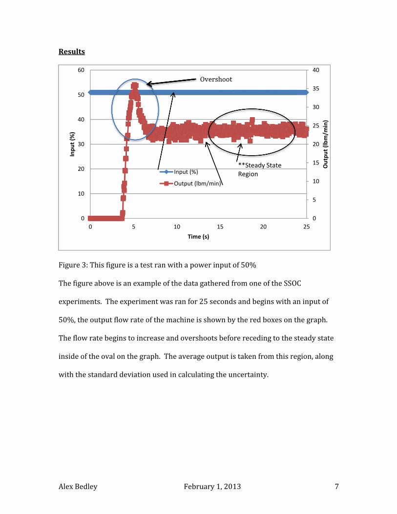
Figure 3: This figure is a test ran with a power input of 50%

The figure above is an example of the data gathered from one of the SSOC

experiments. The experiment was ran for 25 seconds and begins with an input of

50%, the output flow rate of the machine is shown by the red boxes on the graph.

The flow rate begins to increase and overshoots before receding to the steady state

inside of the oval on the graph. The average output is taken from this region, along

with the standard deviation used in calculating the uncertainty.

0

5

10

15

20

25

30

35

40

0

10

20

30

40

50

60

0 5 10 15 20 25

Ou

tpu

t (l

bm

/min

)

Inp

ut

(%)

Time (s)

Input (%)

Output (lbm/min)

**Steady State

Region

Alex Bedley February 1, 2013 8

Input (%)

Output

(lbm/min) Uncertainty

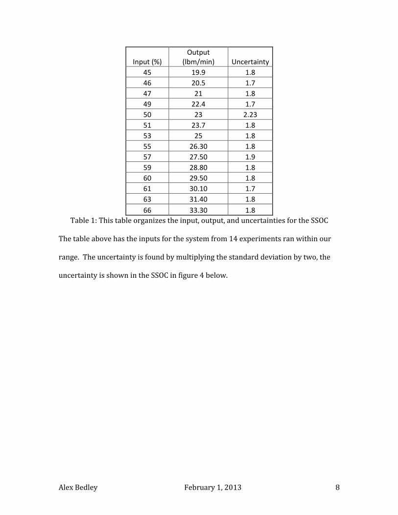
45 19.9 1.8

46 20.5 1.7

47 21 1.8

49 22.4 1.7

50 23 2.23

51 23.7 1.8

53 25 1.8

55 26.30 1.8

57 27.50 1.9

59 28.80 1.8

60 29.50 1.8

61 30.10 1.7

63 31.40 1.8

66 33.30 1.8

Table 1: This table organizes the input, output, and uncertainties for the SSOC

The table above has the inputs for the system from 14 experiments ran within our

range. The uncertainty is found by multiplying the standard deviation by two, the

uncertainty is shown in the SSOC in figure 4 below.

Alex Bedley February 1, 2013 9

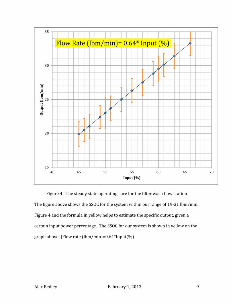
Figure 4: The steady state operating cure for the filter wash flow station

The figure above shows the SSOC for the system within our range of 19-31 lbm/min.

Figure 4 and the formula in yellow helps to estimate the specific output, given a

certain input power percentage. The SSOC for our system is shown in yellow on the

graph above; [Flow rate (lbm/min)=0.64*Input(%)].

Flow Rate (lbm/min)= 0.64* Input (%)

15

20

25

30

35

40 45 50 55 60 65 70

Ou

tpu

t (l

bm

/m

in)

Input (%)

Alex Bedley February 1, 2013 10

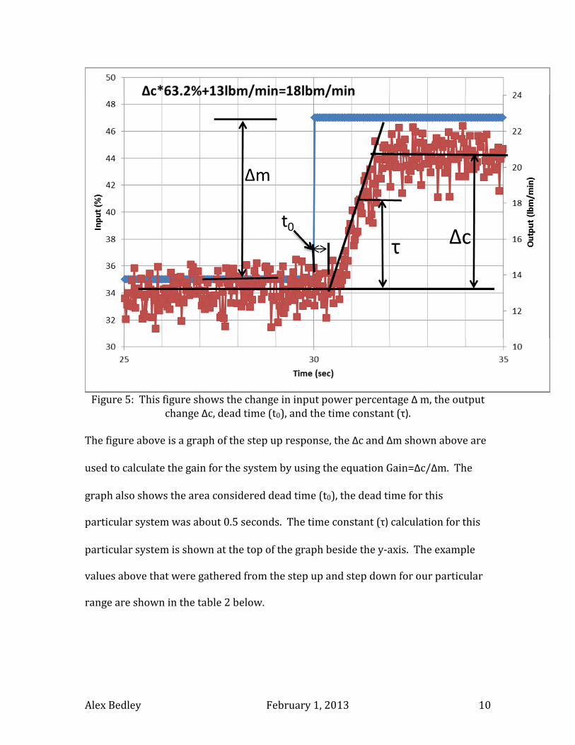
Figure 5: This figure shows the change in input power percentage Δ m, the output

change Δc, dead time (t0), and the time constant (τ).

The figure above is a graph of the step up response, the Δc and Δm shown above are

used to calculate the gain for the system by using the equation Gain=Δc/Δm. The

graph also shows the area considered dead time (t0), the dead time for this

particular system was about 0.5 seconds. The time constant (τ) calculation for this

particular system is shown at the top of the graph beside the y-axis. The example

values above that were gathered from the step up and step down for our particular

range are shown in the table 2 below.

Alex Bedley February 1, 2013 11

Regions Gain up Gain down τ up τ down t0 up t0 down

Low 0.62 0.71 0.83 0.87 0.48 0.57

Medium 0.66 0.63 0.80 0.87 0.57 0.53

High 0.63 0.67 0.77 0.53 0.60 0.67

Uncertainty Gain up Gain down τ up τ down t0 up t0 down

Low 0.09 0.01 0.12 0.12 0.06 0.12

Medium 0.02 0.04 0.20 0.12 0.12 0.12

High 0.12 0.12 0.12 0.23 0.00 0.23

Table 2: Values gathered for gain, time constant, and dead time.

This table is a list of averages for each team member for the gain, time constant and

dead time. The uncertainties for each of the characteristics of the step response are

located in the lower set of tables. These uncertainties are used in the following

figures as (I) shaped bars centered on the top of each colored or textured bar.

Alex Bedley February 1, 2013 12

Figure 6: Gain for the system using the values from table 2 including the uncertainty.

In figures 6, the step up response is shown in the graphs as the blue textured block,

and the step downs are the red boxes. The uncertainties for each system

characteristic are shown in the graphs as the black (I) centered at the top of the

graph as explained before.

0.00

0.10

0.20

0.30

0.40

0.50

0.60

0.70

0.80

0.90

1.00

Low Medium High

Gain (lbm/min/%) Gain up

Gain down

Alex Bedley February 1, 2013 13

Figure 7: Time constant for the system using the values from table 2 including the

uncertainty.

In figures 7, the step up response is shown in the graphs as the blue textured block,

and the step downs are the red boxes. The uncertainties for each system

characteristic are shown in the graphs as the black (I) centered at the top of the

graph as explained before.

0.00

0.20

0.40

0.60

0.80

1.00

1.20

Low Medium High

τ (sec) τ up

τ down

Alex Bedley February 1, 2013 14

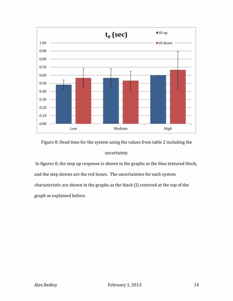
Figure 8: Dead time for the system using the values from table 2 including the

uncertainty.

In figures 8, the step up response is shown in the graphs as the blue textured block,

and the step downs are the red boxes. The uncertainties for each system

characteristic are shown in the graphs as the black (I) centered at the top of the

graph as explained before.

0.00

0.10

0.20

0.30

0.40

0.50

0.60

0.70

0.80

0.90

1.00

Low Medium High

t0 (sec) t0 up

t0 down

Alex Bedley February 1, 2013 15

Discussion

In the first experiment, the steady state operating curve showed that the flow rate

was 0.64*Input (%). For the output range that we were trying to fall within, the

required motor input was between 45-66%. For the flow station, the SSOC shows

that the system is very linear and consistent; this mathematical model gives fairly

accurate results when trying to predict the output for the system when specifying

the input.

In the step response experiment, the results throughout the output range of 19-31

lbm/min, the gains, time constant, and dead time for the system are pretty

consistent from low range to the high range with the uncertainty bars for each set of

data almost falling within the range of the other values for the system characteristic.

The average gain for the system was 0.65 which is very similar to the constant value

of 0.64 obtained in the steady state operating curve. The dead time and time

constant for the system averaged around 0.8 seconds and 0.55 seconds respectively.

The uncertainties were slightly larger in the higher end of our range except for the

step up dead time.

Alex Bedley February 1, 2013 16

Conclusions and Recommendations

The objective of the experiment was to create a steady state operating curve for the

filter wash flow control system with outputs of 27-31 lbm/min with both valves

closed for the entire experiment, and to study three system characteristics for a step

response. The inputs for the system were manipulated in order to control what the

output for the system. The linear fit for the SSOC became Flow rate

(lbm/min)=0.64(lbm/min/%)*Input(%). The linear fit slope of the steady state

operating curve was within a hundredth of the average gain from the step response.

The time constant and dead times throughout the system were similar within the

high, medium, and low sections of our output range. The experiments ran well, the

system took a few experiments to warm up and give consistent data; overall the

system provided usable data.

Alex Bedley February 1, 2013 17

Appendices

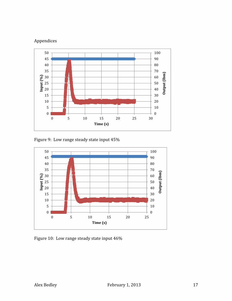
Figure 9: Low range steady state input 45%

Figure 10: Low range steady state input 46%

0

10

20

30

40

50

60

70

80

90

100

0

5

10

15

20

25

30

35

40

45

50

0 5 10 15 20 25 30

Ou

tpu

t (l

bm

)

Inp

ut

(%)

Time (s)

0

10

20

30

40

50

60

70

80

90

100

0

5

10

15

20

25

30

35

40

45

50

0 5 10 15 20 25

Ou

tpu

t (l

bm

)

Inp

ut

(%)

Time (s)

Alex Bedley February 1, 2013 18

Figure 11: Low range steady state input 46%

Figure 12: Mid range steady state input 49%

0

5

10

15

20

25

30

35

40

0

5

10

15

20

25

30

35

40

45

50

0 5 10 15 20 25

Ou

tpu

t (l

bm

)

Inp

ut

(%)

Time (s)

0

10

20

30

40

50

60

70

80

90

0

10

20

30

40

50

60

0 5 10 15 20 25

Ou

tpu

t (l

bm

)

Inp

ut

(%)

Time (s)

Alex Bedley February 1, 2013 19

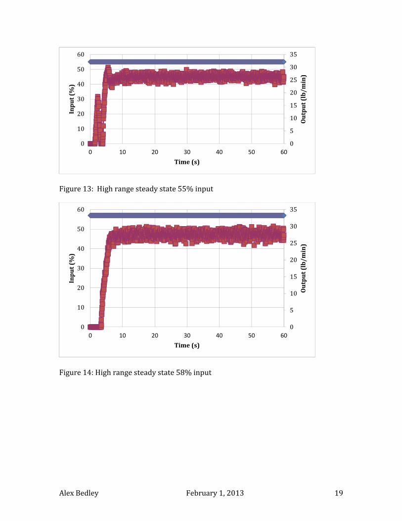
Figure 13: High range steady state 55% input

Figure 14: High range steady state 58% input

0

5

10

15

20

25

30

35

0

10

20

30

40

50

60

0 10 20 30 40 50 60

Ou

tpu

t (l

b/

min

)

Inp

ut

(%)

Time (s)

0

5

10

15

20

25

30

35

0

10

20

30

40

50

60

0 10 20 30 40 50 60

Ou

tpu

t (l

b/

min

)

Inp

ut

(%)

Time (s)

Alex Bedley February 1, 2013 20

Figure 15: High range steady state 60% input

Figure 16: High range steady state 61% input

0

5

10

15

20

25

30

35

40

45

50

0

10

20

30

40

50

60

70

0 10 20 30 40 50 60

Ou

tpu

t (l

b/

min

)

Inp

ut

(%)

Time (s)

0

5

10

15

20

25

30

35

0

10

20

30

40

50

60

70

0 10 20 30 40 50 60

Ou

tpu

t (l

b/

min

)

Inp

ut

(%)

Time (s)

Alex Bedley February 1, 2013 21

Figure 17: High range steady state input 61%

Figure 18: High range steady state 63% input

0

10

20

30

40

50

60

70

80

90

0

10

20

30

40

50

60

70

0 10 20 30 40 50 60

Ou

tpu

t (l

b/

min

)

Inp

ut

(%)

Time (s)

0

5

10

15

20

25

30

35

40

0

10

20

30

40

50

60

70

0 10 20 30 40 50 60

Ou

tpu

t (l

b/

min

)

Inp

ut

(%)

Time (s)

Alex Bedley February 1, 2013 22

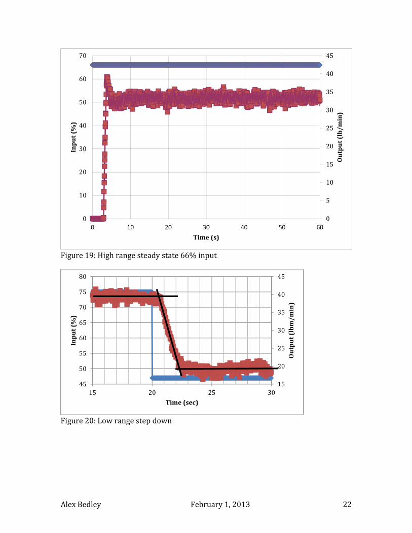
Figure 19: High range steady state 66% input

Figure 20: Low range step down

0

5

10

15

20

25

30

35

40

45

0

10

20

30

40

50

60

70

0 10 20 30 40 50 60

Ou

tpu

t (l

b/

min

)

Inp

ut

(%)

Time (s)

15

20

25

30

35

40

45

45

50

55

60

65

70

75

80

15 20 25 30

Ou

tpu

t (l

bm

/m

in)

Inp

ut

(%)

Time (sec)

Alex Bedley February 1, 2013 23

Figure 21: Low range step down

Figure 22: Low range step down

15

20

25

30

35

40

45

45

50

55

60

65

70

75

80

15 20 25 30

Ou

tpu

t (l

bm

/m

in)

Inp

ut

(%)

Time (sec)

15

20

25

30

35

40

45

45

50

55

60

65

70

75

80

15 20 25 30

Ou

tpu

t (l

bm

/m

in)

Inp

ut

(%)

Time (sec)

Alex Bedley February 1, 2013 24

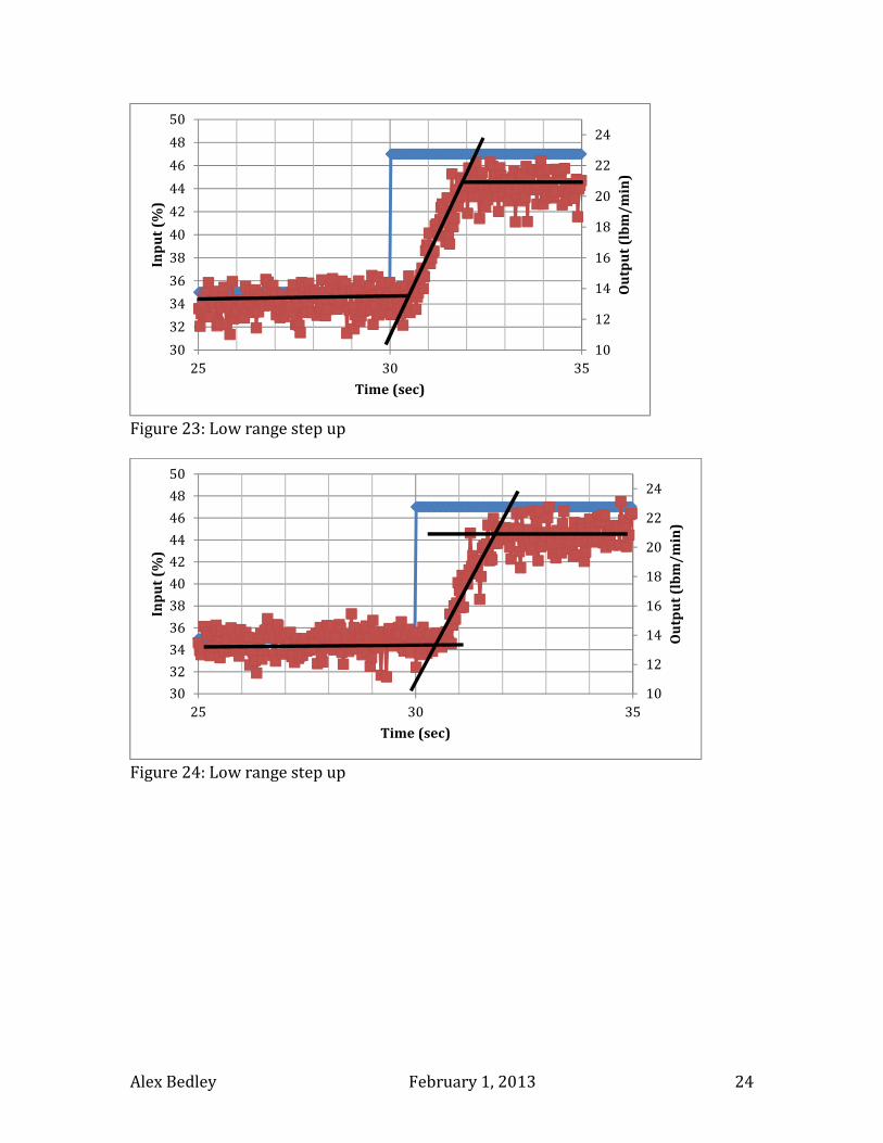
Figure 23: Low range step up

Figure 24: Low range step up

10

12

14

16

18

20

22

24

30

32

34

36

38

40

42

44

46

48

50

25 30 35

Ou

tpu

t (l

bm

/m

in)

Inp

ut

(%)

Time (sec)

10

12

14

16

18

20

22

24

30

32

34

36

38

40

42

44

46

48

50

25 30 35

Ou

tpu

t (l

bm

/m

in)

Inp

ut

(%)

Time (sec)

Alex Bedley February 1, 2013 25

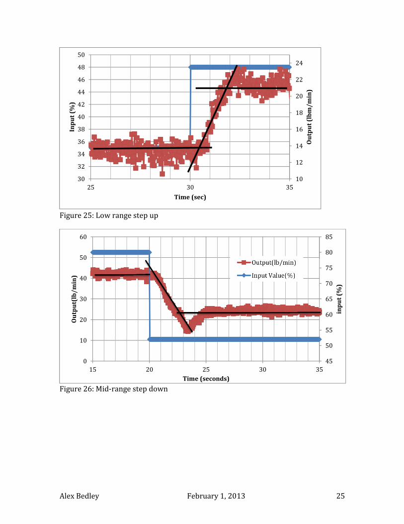
Figure 25: Low range step up

Figure 26: Mid-range step down

10

12

14

16

18

20

22

24

30

32

34

36

38

40

42

44

46

48

50

25 30 35

Ou

tpu

t (l

bm

/m

in)

Inp

ut

(%)

Time (sec)

45

50

55

60

65

70

75

80

85

0

10

20

30

40

50

60

15 20 25 30 35

inp

ut

(%)

Ou

tpu

t(lb

/m

in)

Time (seconds)

Output(lb/min)

Input Value(%)

Alex Bedley February 1, 2013 26

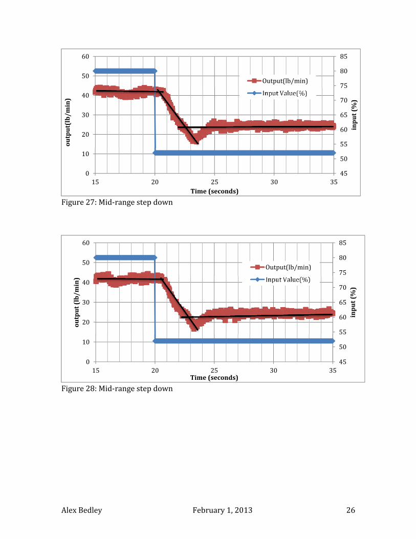
Figure 27: Mid-range step down

Figure 28: Mid-range step down

45

50

55

60

65

70

75

80

85

0

10

20

30

40

50

60

15 20 25 30 35

inp

ut

(%)

ou

tpu

t(lb

/m

in)

Time (seconds)

Output(lb/min)

Input Value(%)

45

50

55

60

65

70

75

80

85

0

10

20

30

40

50

60

15 20 25 30 35

inp

ut

(%)

ou

tpu

t (l

b/

min

)

Time (seconds)

Output(lb/min)

Input Value(%)

Alex Bedley February 1, 2013 27

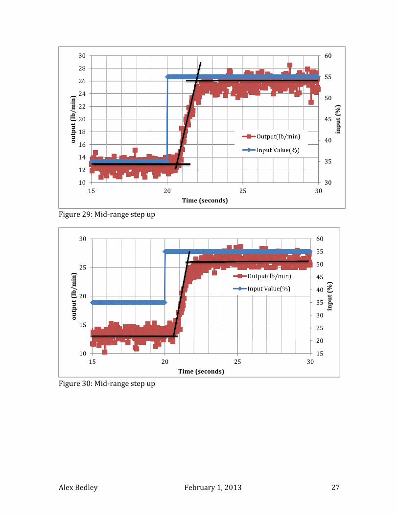
Figure 29: Mid-range step up

Figure 30: Mid-range step up

30

35

40

45

50

55

60

10

12

14

16

18

20

22

24

26

28

30

15 20 25 30

inp

ut

(%)

ou

tpu

t (l

b/

min

)

Time (seconds)

Output(lb/min)

Input Value(%)

15

20

25

30

35

40

45

50

55

60

10

15

20

25

30

15 20 25 30

inp

ut

(%)

ou

tpu

t (l

b/

min

)

Time (seconds)

Output(lb/min)

Input Value(%)

Alex Bedley February 1, 2013 28

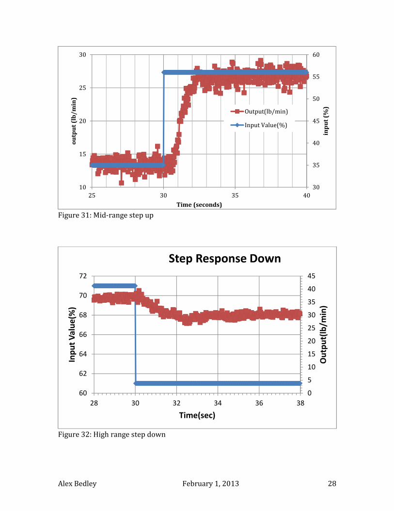
Figure 31: Mid-range step up

Figure 32: High range step down

30

35

40

45

50

55

60

10

15

20

25

30

25 30 35 40

inp

ut

(%)

ou

tpu

t (l

b/

min

)

Time (seconds)

Output(lb/min)

Input Value(%)

0

5

10

15

20

25

30

35

40

45

60

62

64

66

68

70

72

28 30 32 34 36 38

Ou

tpu

t(lb

/min

)

Inp

ut

Va

lue

(%)

Time(sec)

Step Response Down

Alex Bedley February 1, 2013 29

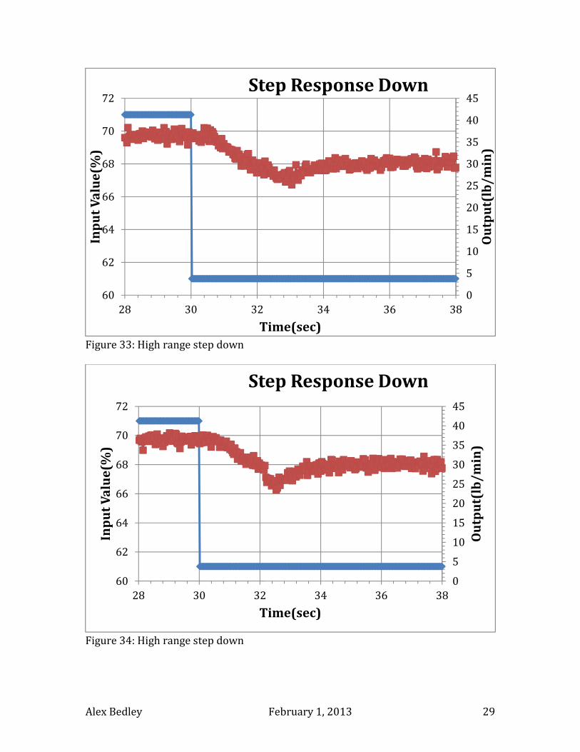
Figure 33: High range step down

Figure 34: High range step down

0

5

10

15

20

25

30

35

40

45

60

62

64

66

68

70

72

28 30 32 34 36 38

Ou

tpu

t(lb

/m

in)

Inp

ut

Va

lue

(%)

Time(sec)

Step Response Down

0

5

10

15

20

25

30

35

40

45

60

62

64

66

68

70

72

28 30 32 34 36 38

Ou

tpu

t(lb

/m

in)

Inp

ut

Va

lue

(%)

Time(sec)

Step Response Down

Alex Bedley February 1, 2013 30

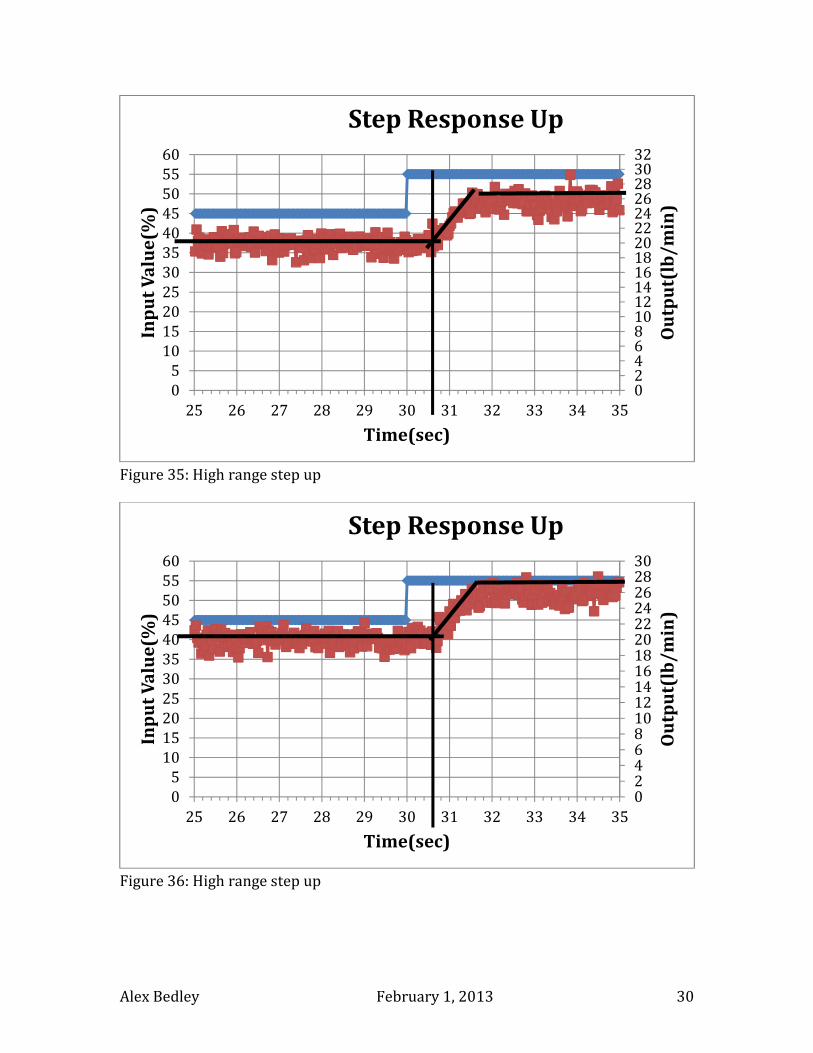
Figure 35: High range step up

Figure 36: High range step up

02468101214161820222426283032

0

5

10

15

20

25

30

35

40

45

50

55

60

25 26 27 28 29 30 31 32 33 34 35

Ou

tpu

t(lb

/m

in)

Inp

ut

Va

lue

(%)

Time(sec)

Step Response Up

024681012141618202224262830

0

5

10

15

20

25

30

35

40

45

50

55

60

25 26 27 28 29 30 31 32 33 34 35

Ou

tpu

t(lb

/m

in)

Inp

ut

Va

lue

(%)

Time(sec)

Step Response Up

Alex Bedley February 1, 2013 31

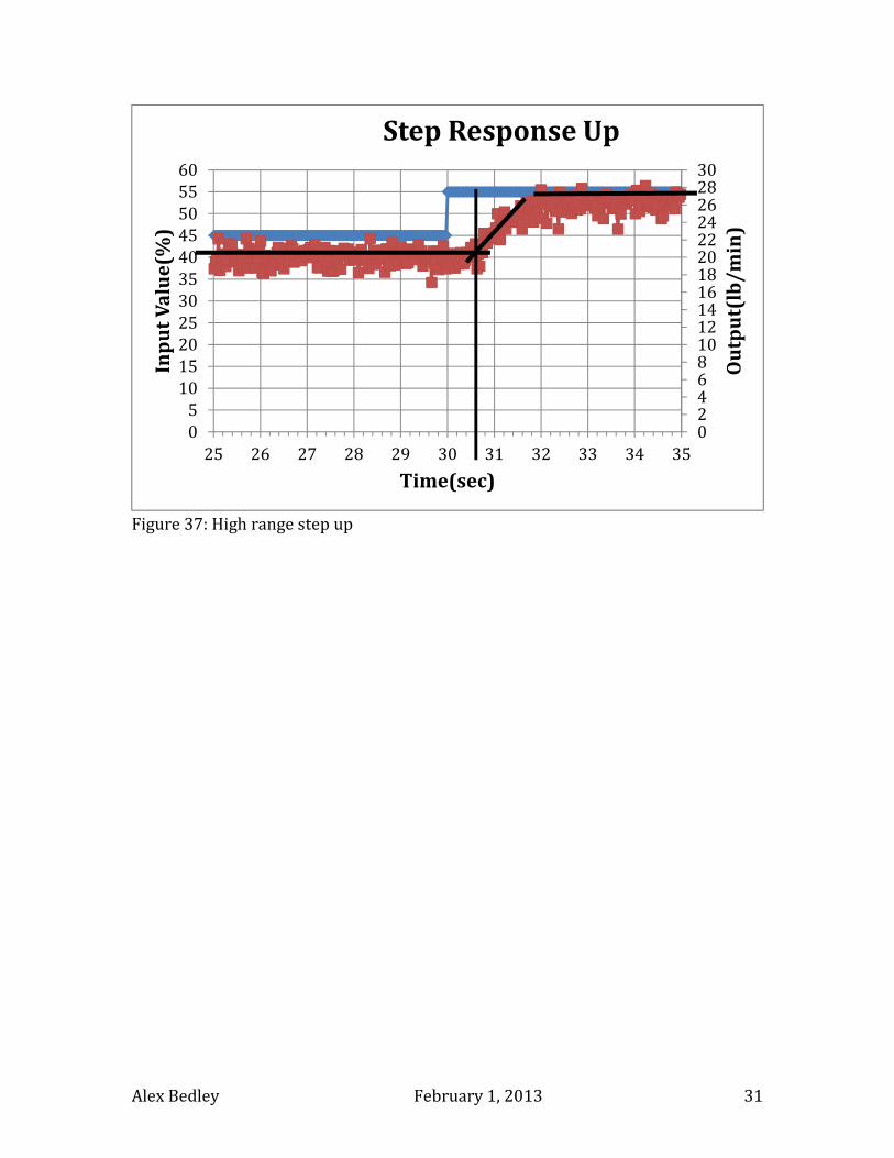
Figure 37: High range step up

024681012141618202224262830

0

5

10

15

20

25

30

35

40

45

50

55

60

25 26 27 28 29 30 31 32 33 34 35

Ou

tpu

t(lb

/m

in)

Inp

ut

Va

lue

(%)

Time(sec)

Step Response Up