Statistik Bisnis 2 - devilia.staff.telkomuniversity.ac.id
66
Statistik Bisnis Week 11 Two-Sample Tests
Transcript of Statistik Bisnis 2 - devilia.staff.telkomuniversity.ac.id

Statistik Bisnis
Week 11
Two-Sample Tests
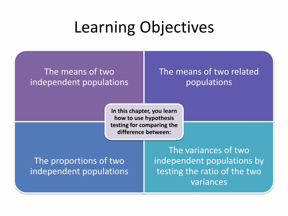
Learning Objectives
The means of two independent populations
The means of two related populations
The proportions of two independent populations
The variances of two independent populations by testing the ratio of the two
variances
In this chapter, you learn how to use hypothesis
testing for comparing the difference between:

Two-Sample Tests
Two-Sample Tests
Population Means
Independent Samples
unknown, assumed
equal
unknown, assumed unequal
Related Samples
Population Proportions
Population Variances

Difference Between Two Means
Goal: Test hypothesis or form a confidence interval for the difference between two population means, μ1 – μ2
The point estimate for the difference is
X1 – X2
Independent Samples
unknown, assumed
equal
unknown, assumed unequal

Difference Between Two Means: Independent Samples
Different data sources • Unrelated • Independent
– Sample selected from one population has no effect on the sample selected from the other population
Use Sp to estimate unknown σ. Use a Pooled-Variance t test.
Use S1 and S2 to estimate unknown σ1 and σ2. Use a Separate-Variance t test.
Independent Samples
unknown, assumed
equal
unknown, assumed unequal
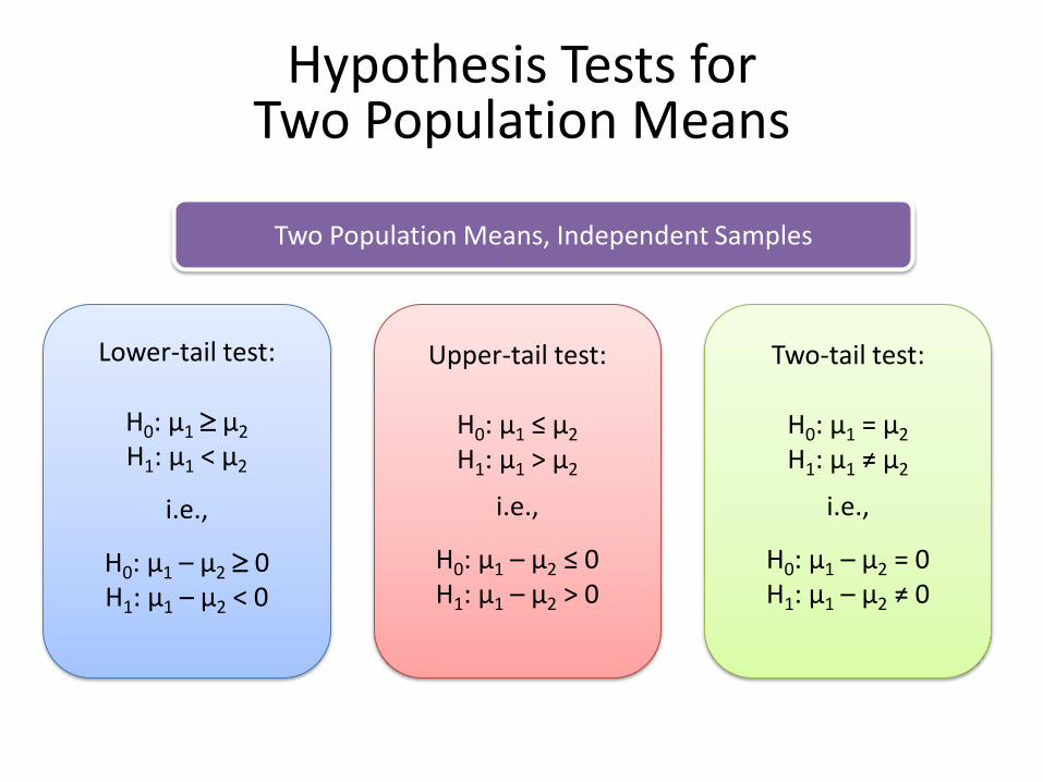
Hypothesis Tests for Two Population Means
Upper-tail test:
H0: μ1 ≤ μ2
H1: μ1 > μ2
i.e.,
H0: μ1 – μ2 ≤ 0 H1: μ1 – μ2 > 0
Lower-tail test:
H0: μ1 μ2 H1: μ1 < μ2
i.e.,
H0: μ1 – μ2 0 H1: μ1 – μ2 < 0
Two-tail test:
H0: μ1 = μ2
H1: μ1 ≠ μ2
i.e.,
H0: μ1 – μ2 = 0 H1: μ1 – μ2 ≠ 0
Two Population Means, Independent Samples
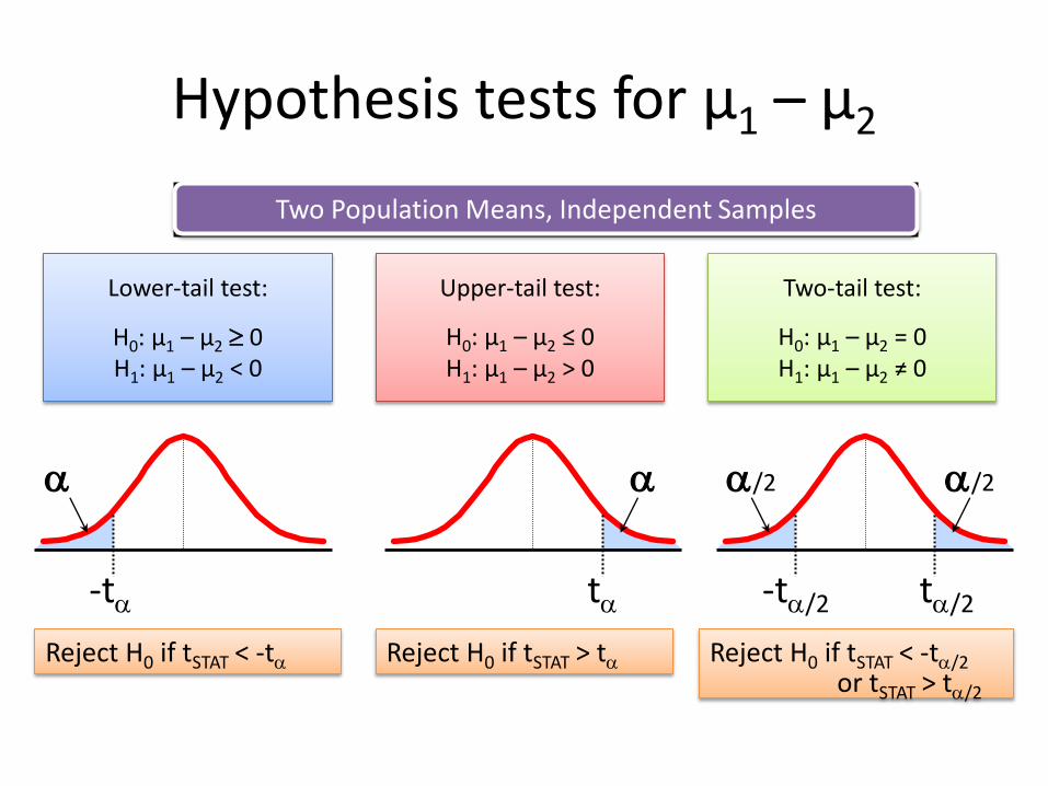
Upper-tail test:
H0: μ1 – μ2 ≤ 0 H1: μ1 – μ2 > 0
Lower-tail test:
H0: μ1 – μ2 0 H1: μ1 – μ2 < 0
Two Population Means, Independent Samples
Two-tail test:
H0: μ1 – μ2 = 0 H1: μ1 – μ2 ≠ 0
a a/2 a/2 a
-ta -ta/2 ta ta/2
Reject H0 if tSTAT < -ta Reject H0 if tSTAT > ta Reject H0 if tSTAT < -ta/2
or tSTAT > ta/2
Hypothesis tests for μ1 – μ2

Hypothesis tests for µ1 - µ2 with σ1 and σ2 unknown and assumed equal
Assumptions:
Samples are randomly and independently drawn
Populations are normally distributed or both sample sizes are at least 30 Population variances are unknown but assumed equal
Independent Samples
unknown, assumed
equal
unknown, assumed unequal

Hypothesis tests for µ1 - µ2 with σ1 and σ2 unknown and assumed equal
• The pooled variance is:
• The test statistic is:
• Where tSTAT has d.f. = (n1 + n2 – 2)
(continued)
1)n()1(n
S1nS1nS
21
2
22
2
112
p
21
2
p
2121
STAT
n
1
n
1S
μμXXt
Independent Samples
unknown, assumed
equal
unknown, assumed unequal

21
2
p/221
n
1
n
1SXX at
The confidence interval for
μ1 – μ2 is:
Where tα/2 has d.f. = n1 + n2 – 2
Confidence interval for µ1 - µ2 with σ1 and σ2 unknown and assumed equal
Independent Samples
unknown, assumed
equal
unknown, assumed unequal

Pooled-Variance t Test Example
Anda adalah seorang analis keuangan dan ingin mengetahui apakah terdapat perbedaan hasil dividen antara saham yang terdaftar di NYSE & NASDAQ? Anda mengumpulkan data:
NYSE NASDAQ Jumlah 21 25 Rata-rata sampel 3.27 2.53 Std dev sampel 1.30 1.16
Dengan mengasumsikan bahwa kedua populasi berdistribusi normal dengan variansi sama, apakah terdapat perbedaan pada rata-rata hasil (a = 0.05)?

Pooled-Variance t Test Example: Calculating the Test Statistic
1.5021
1)25(1)-(21
1.161251.30121
1)n()1(n
1n1n22
21
2
22
2
112
SSSP
2.040
25
1
21
15021.1
02.533.27
n
1
n
1S
μμXXt
21
2
p
2121
STAT
The test statistic is:
(continued)
H0: μ1 - μ2 = 0 i.e. (μ1 = μ2) H1: μ1 - μ2 ≠ 0 i.e. (μ1 ≠ μ2)
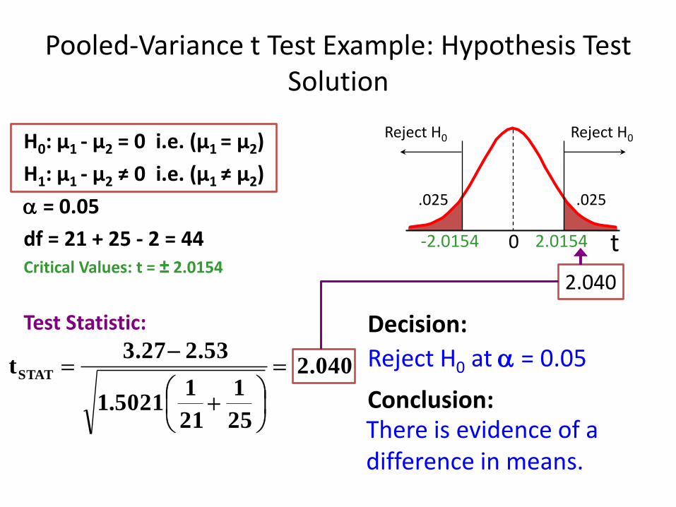
Pooled-Variance t Test Example: Hypothesis Test Solution
H0: μ1 - μ2 = 0 i.e. (μ1 = μ2)
H1: μ1 - μ2 ≠ 0 i.e. (μ1 ≠ μ2)
a = 0.05
df = 21 + 25 - 2 = 44 Critical Values: t = ± 2.0154
Test Statistic: Decision:
Conclusion:
Reject H0 at a = 0.05
There is evidence of a difference in means.
t 0 2.0154 -2.0154
.025
Reject H0 Reject H0
.025
2.040
2.040
25
1
21
15021.1
2.533.27tSTAT

Pooled-Variance t Test Example: Confidence Interval for µ1 - µ2
Since we rejected H0 can we be 95% confident that µNYSE > µNASDAQ?
95% Confidence Interval for µNYSE - µNASDAQ
Since 0 is less than the entire interval, we can be 95% confident that µNYSE > µNASDAQ
)471.1,009.0(3628.00154.274.0 n
1
n
1SXX
21
2
p/221
at
DCOVA

Hypothesis tests for µ1 - µ2 with σ1 and σ2 unknown, not assumed equal
Assumptions:
Samples are randomly and independently drawn
Populations are normally distributed or both sample sizes are at least 30 Population variances are unknown and cannot be assumed to be equal
Independent Samples
unknown, assumed
equal
unknown, assumed unequal
(continued)
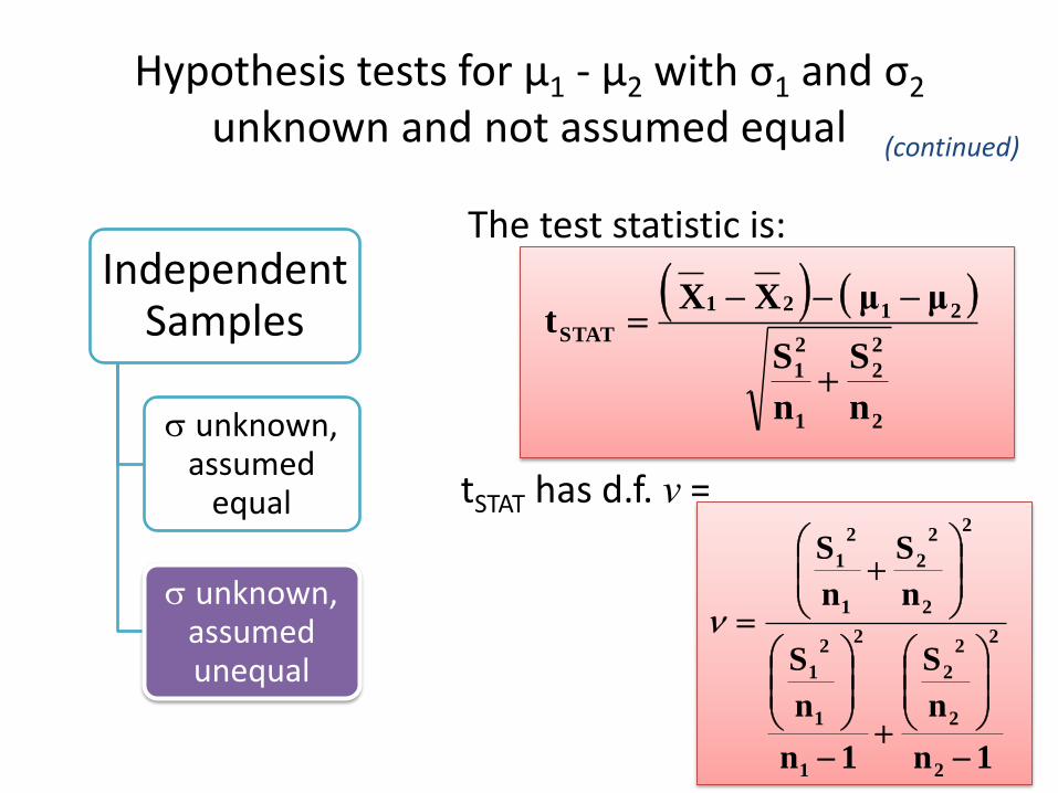
Hypothesis tests for µ1 - µ2 with σ1 and σ2 unknown and not assumed equal
1n
n
S
1n
n
S
n
S
n
S
2
2
2
2
2
1
2
1
2
1
2
2
2
2
1
2
1
The test statistic is:
2
2
2
1
2
1
2121
STAT
n
S
n
S
μμXXt
tSTAT has d.f. ν =
Independent Samples
unknown, assumed
equal
unknown, assumed unequal

EXERCISE
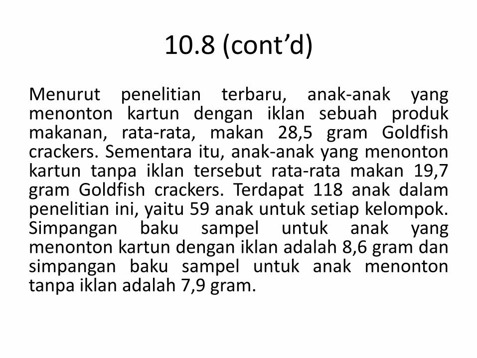
10.8 (cont’d)
Menurut penelitian terbaru, anak-anak yang menonton kartun dengan iklan sebuah produk makanan, rata-rata, makan 28,5 gram Goldfish crackers. Sementara itu, anak-anak yang menonton kartun tanpa iklan tersebut rata-rata makan 19,7 gram Goldfish crackers. Terdapat 118 anak dalam penelitian ini, yaitu 59 anak untuk setiap kelompok. Simpangan baku sampel untuk anak yang menonton kartun dengan iklan adalah 8,6 gram dan simpangan baku sampel untuk anak menonton tanpa iklan adalah 7,9 gram.

10.8
Dengan mengasumsikan variansi populasi sama dan α=0,05, apakah terdapat cukup bukti bahwa rata-rata jumlah Goldfish crackers yang dimakan oleh anak-anak yang menonton kartun dengan iklan lebih tinggi?

10.10 (cont’d)
Computer Anxiety Rating Scale (CARS) mengukur tingkat kecemasan terhadap komputer (computer anxiety), dengan skala dari 20 (tidak ada kecemasan) hingga 100 (sangat cemas). Peneliti dari Miami University menyebarkan CARS pada 172 mahasiswa bisnis. Salah satu tujuan dari penelitian tersebut adalah menentukan apakah terdapat perbedaan tingkat kecemasan komputer yang dirasakan oleh mahasiswa bisnis pria dan wanita. Mereka menemukan data berikut:
Pria Wanita
𝑋 40,26 36,85 s 13,35 9,42 n 100 72

10.10
Dengan tingkat signifikansi 0.05, apakah terdapat bukti bahwa kecemasan komputer yang dirasakan oleh mahasiswa bisnis wanita berbeda dari yang dirasakan oleh mahasiswa bisnis pria?

10.13
Sebuah cabang Bank Mandiri yang terletak di area komersial ingin meningkatkan pelayanannya dengan memperpendek waktu tunggu. Berikut adalah data waktu tunggu untuk dilayani pada cabang Bank Mandiri tersebut (data diambil dari sampel 15 orang nasabah):
Waktu tunggu(Bank 1) Rata-rata 4,29
Standar Deviasi 1,64

10.13
Misalkan terdapat cabang lain yang terletak di area perumahan juga ingin memperpendek waktu tunggu pelayanannya. Pada bank ini dipilih juga sebuah sampel yang terdiri dari 15 orang nasabah, dengan hasil sebagai berikut:
Waktu Tunggu (Bank 2)
Rata-rata 7,11
Standar Deviasi 2,08

10.13
Dengan mengasumsikan bahwa variansi populasi kedua bank tersebut tidak sama, apakah terdapat bukti yang menunjukkan rata-rata waktu menunggu di kedua cabang tersebut berbeda? (Gunakan α = 0,05)

10.16 (cont’d)
Apakah anak-anak menggunakan telepon selular? Sepertinya demikian, menurut penelitian baru-baru ini, pengguna telepon selular berusia dibawah 12 tahun rata-rata melakukan 137 panggilan telepon per bulan. Cukup tinggi, jika dibandingkan dengan 231 panggilan telepon per bulan yang dilakukan oleh pengguna telepon selular berusia 13 hingga 17 tahun.

10.16 (cont’d)
Misalkan hasil tersebut diambil dari sampel 50 orang pengguna telepon selular untuk setiap grup pengguna dan simpangan baku sampel pengguna telepon selular berusia dibawah 12 tahun adalah 51,7 panggilan telepon per bulan dan simpangan baku sampel pengguna telepon selular berusia 13 hingga 17 tahun adalah 67,6 panggilan telepon per bulan.

10.16
Dengan mengasumsikan bahwa variansi populasi dari pengguna telepon selular adalah sama, adakah bukti yang menunjukkan bahwa terdapat perbedaan rata-rata penggunaan telepon selular antara kelompok usia dibawah 12 tahun dan kepompok usia 13 hingga 17 tahun? (Gunakan tingkat signifikansi 0,05.)

Two-Sample Tests
Two-Sample Tests
Population Means
Independent Samples
unknown, assumed
equal
unknown, assumed unequal
Related Samples
Population Proportions
Population Variances
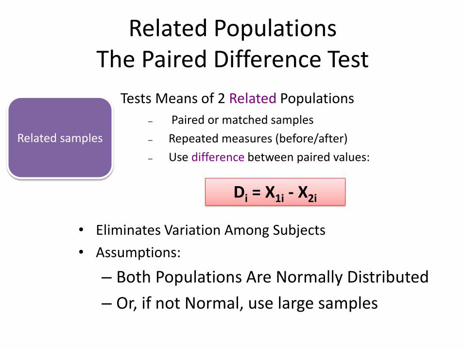
Related Populations The Paired Difference Test
Tests Means of 2 Related Populations
– Paired or matched samples
– Repeated measures (before/after)
– Use difference between paired values:
• Eliminates Variation Among Subjects
• Assumptions:
– Both Populations Are Normally Distributed
– Or, if not Normal, use large samples
Related samples
Di = X1i - X2i

Related Populations The Paired Difference Test
The ith paired difference is Di , where
Di = X1i - X2i
The point estimate for the paired Difference population mean μD is D :
n
D
D
n
1i
i
n is the number of pairs in the paired sample
1n
)D(D
S
n
1i
2
i
D
The sample standard deviation is SD
(continued)
Related samples
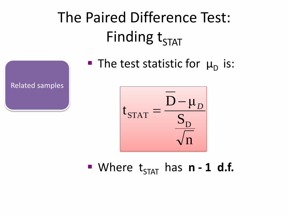
The Paired Difference Test: Finding tSTAT
The test statistic for μD is:
Where tSTAT has n - 1 d.f.
n
S
μDt
DSTAT
D
Related samples

Upper-tail test:
H0: μD ≤ 0
H1: μD > 0
Lower-tail test:
H0: μD 0 H1: μD < 0
Two-tail test:
H0: μD = 0
H1: μD ≠ 0
Paired Samples
The Paired Difference Test: Possible Hypotheses
a a/2 a/2 a
-ta -ta/2 ta ta/2
Reject H0 if tSTAT < -ta Reject H0 if tSTAT > ta Reject H0 if tSTAT < -ta/2
or tSTAT > ta/2
Where tSTAT has n - 1 d.f.
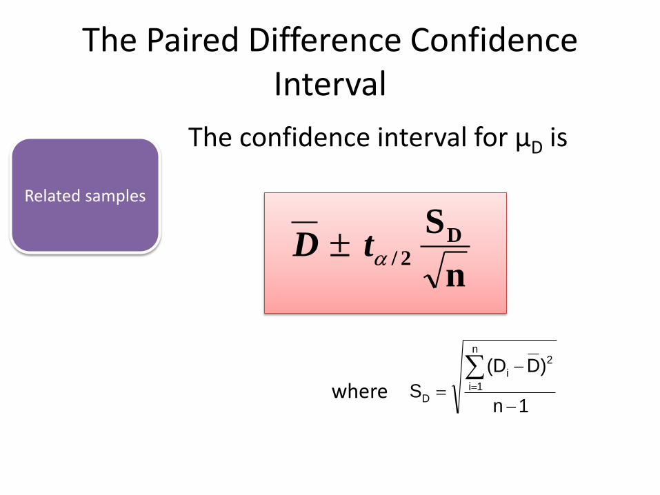
The Paired Difference Confidence Interval
The confidence interval for μD is
1n
)D(D
S
n
1i
2
i
D
n
SD2/atD
where
Related samples

Paired Difference Test: Example
Misalkan anda mengirimkan karyawan anda untuk mengikuti pelatihan “customer service”. Apakah pelatihan ini mempengaruhi jumlah keluhan yang masuk? Anda mengumpulkan data sebagai berikut:
Jumlah Keluhan: Karyawan Sebelum Sesudah C.B. 6 4
T.F. 20 6
M.H. 3 2
R.K. 0 0
M.O. 4 0

Paired Difference Test: Example
Misalkan anda mengirimkan karyawan anda untuk mengikuti pelatihan “customer service”. Apakah pelatihan ini mempengaruhi jumlah keluhan yang masuk? Anda mengumpulkan data sebagai berikut:
Jumlah Keluhan: (2) - (1) Karyawan Sebelum (1) Sesudah (2) Selisih, Di C.B. 6 4 - 2
T.F. 20 6 -14
M.H. 3 2 - 1
R.K. 0 0 0
M.O. 4 0 - 4
-21
D = Di
n
5.67
1n
)D(DS
2
i
D
= -4.2

Paired Difference Test: Solution
• Has the training made a difference in the number of complaints (at the 0.01 level)?
- 4.2 D =
1.6655.67/
04.2
n/S
μt
D
STATD
D
H0: μD = 0 H1: μD 0
Test Statistic:
t0.005 = ± 4.604
d.f. = n - 1 = 4
Reject
a/2
- 4.604 4.604
Decision: Do not reject H0
(tstat is not in the reject region)
Conclusion: There is insufficient evidence there is significant change in the number of complaints.
Reject
a/2
- 1.66 a = .01

EXERCISE

10.20 (cont’d)
Sembilan ahli memberi penilaian pada dua merek kopi Kolombia dalam sebuah percobaan taste-testing. Sebuah rating berskala 7 (1 = sangat tidak memuaskan, 7 = sangat memuaskan) diberikan untuk empat karakteristik: rasa, aroma, richness, dan keasaman. Data berikut menunjukkan total rating dari keempat karakteristik tersebut.
Merek Ahli A B C.C. 24 26 S.E. 27 27 E.G. 19 22 B.L. 24 27 C.M. 22 25 C.N. 26 27 G.N. 27 26 R.M. 25 27 P.V. 22 23

10.20
Dengan tingkat signifikansi 0,05, adakah bukti yang menunjukkan bahwa rata-rata rating antara kedua merek tersebut berbeda?

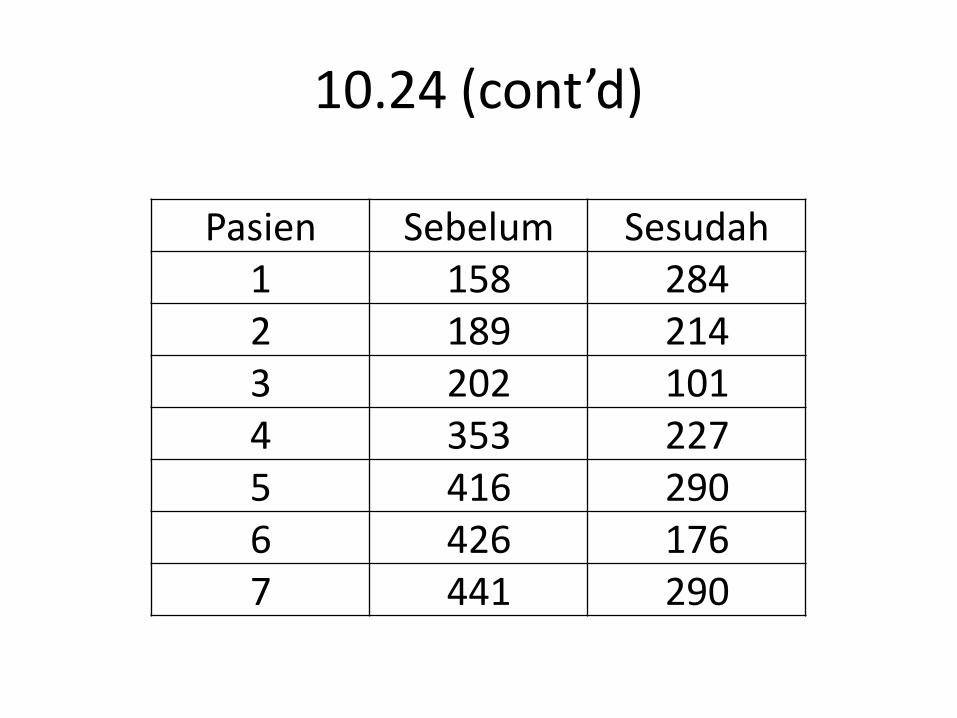
10.24 (cont’d)
Kanker plasma darah (Multiple myeloma), dapat diketahui dari peningkatan pembentukkan pembuluh darah (angiogenesis) pada sumsung tulang yang merupakah faktor penentu keberlangsungan hidup penderitanya. Salah satu pengobatan untuk penyakit ini adala transplantasi sel induk (stem cell). Berikut merupakan data kepadatan pembuluh darah pada sumsum tulang pada pasien yang telah menyelesaikan prosedur transplantasi sel induk (diukur dengan tes darah dan urin).
10.24 (cont’d)
Pasien Sebelum Sesudah 1 158 284 2 189 214 3 202 101 4 353 227 5 416 290 6 426 176 7 441 290
10.24
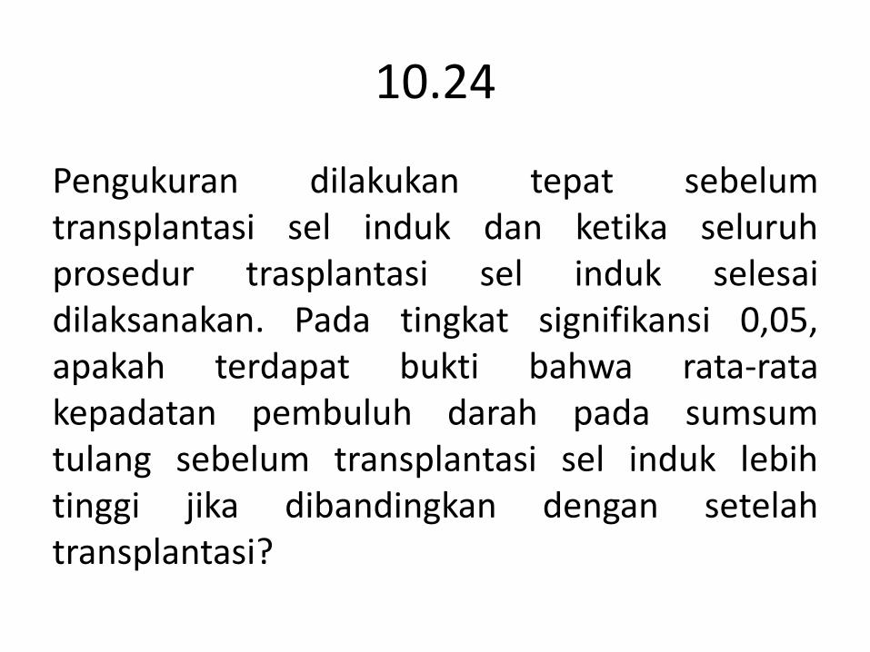
Pengukuran dilakukan tepat sebelum transplantasi sel induk dan ketika seluruh prosedur trasplantasi sel induk selesai dilaksanakan. Pada tingkat signifikansi 0,05, apakah terdapat bukti bahwa rata-rata kepadatan pembuluh darah pada sumsum tulang sebelum transplantasi sel induk lebih tinggi jika dibandingkan dengan setelah transplantasi?

Two-Sample Tests
Two-Sample Tests
Population Means
Independent Samples
unknown, assumed
equal
unknown, assumed unequal
Related Samples
Population Proportions
Population Variances

Two Population Proportions
Goal: test a hypothesis or form a confidence interval for the difference between two population proportions,
π1 – π2
The point estimate for the difference is 21 pp
Population proportions

Two Population Proportions
21
21
nn
XX
p
The pooled estimate for the overall proportion is:
where X1 and X2 are the number of items of interest in samples 1 and 2
In the null hypothesis we assume the null
hypothesis is true, so we assume π1 = π2 and
pool the two sample estimates Population proportions
Two Population Proportions
21
2121
11)1(
nnpp
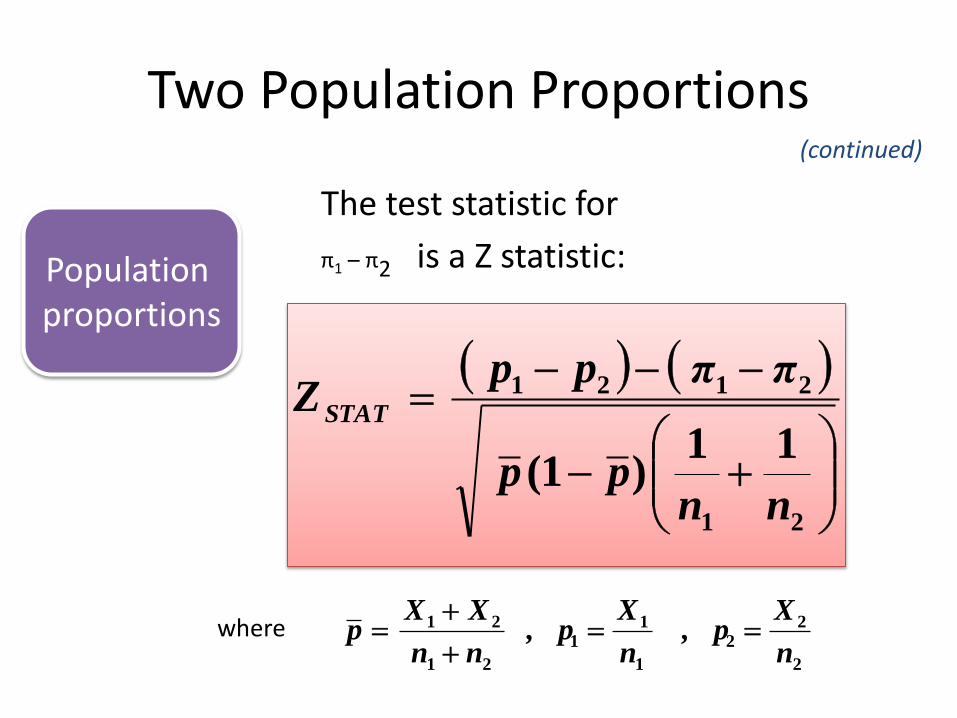
ππppZSTAT
The test statistic for
π1 – π2 is a Z statistic:
(continued)
2
22
1
11
21
21
n
X , p
n
X , p
nn
XXp
where
Population proportions

Upper-tail test:
H0: π1 ≤ π2
H1: π1 > π2
i.e.,
H0: π1 – π2 ≤ 0 H1: π1 – π2 > 0
Lower-tail test:
H0: π1 π2 H1: π1 < π2
i.e.,
H0: π1 – π2 0 H1: π1 – π2 < 0
Hypothesis Tests for Two Population Proportions
Population proportions
Two-tail test:
H0: π1 = π2
H1: π1 ≠ π2
i.e.,
H0: π1 – π2 = 0 H1: π1 – π2 ≠ 0

Upper-tail test:
H0: π1 – π2 ≤ 0 H1: π1 – π2 > 0
Lower-tail test:
H0: π1 – π2 0 H1: π1 – π2 < 0
Hypothesis Tests for Two Population Proportions
Population proportions
Two-tail test:
H0: π1 – π2 = 0 H1: π1 – π2 ≠ 0
a a/2 a/2 a
-za -za/2 za za/2
Reject H0 if ZSTAT < -Za Reject H0 if ZSTAT > Za Reject H0 if ZSTAT < -Za/2
or ZSTAT > Za/2
(continued)
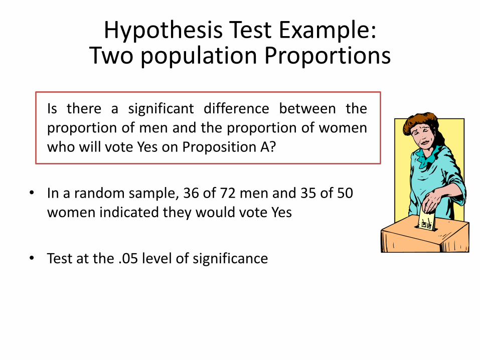
Hypothesis Test Example: Two population Proportions
Is there a significant difference between the proportion of men and the proportion of women who will vote Yes on Proposition A?
• In a random sample, 36 of 72 men and 35 of 50 women indicated they would vote Yes
• Test at the .05 level of significance

Hypothesis Test Example: Two population Proportions
• The hypothesis test is: H0: π1 – π2 = 0 (the two proportions are equal) H1: π1 – π2 ≠ 0 (there is a significant difference between proportions)
The sample proportions are:
Men: p1 = 36/72 = 0.50
Women: p2 = 35/50 = 0.70
5820122
71
5072
3536
21
21 .nn
XXp
The pooled estimate for the overall proportion is:
(continued)
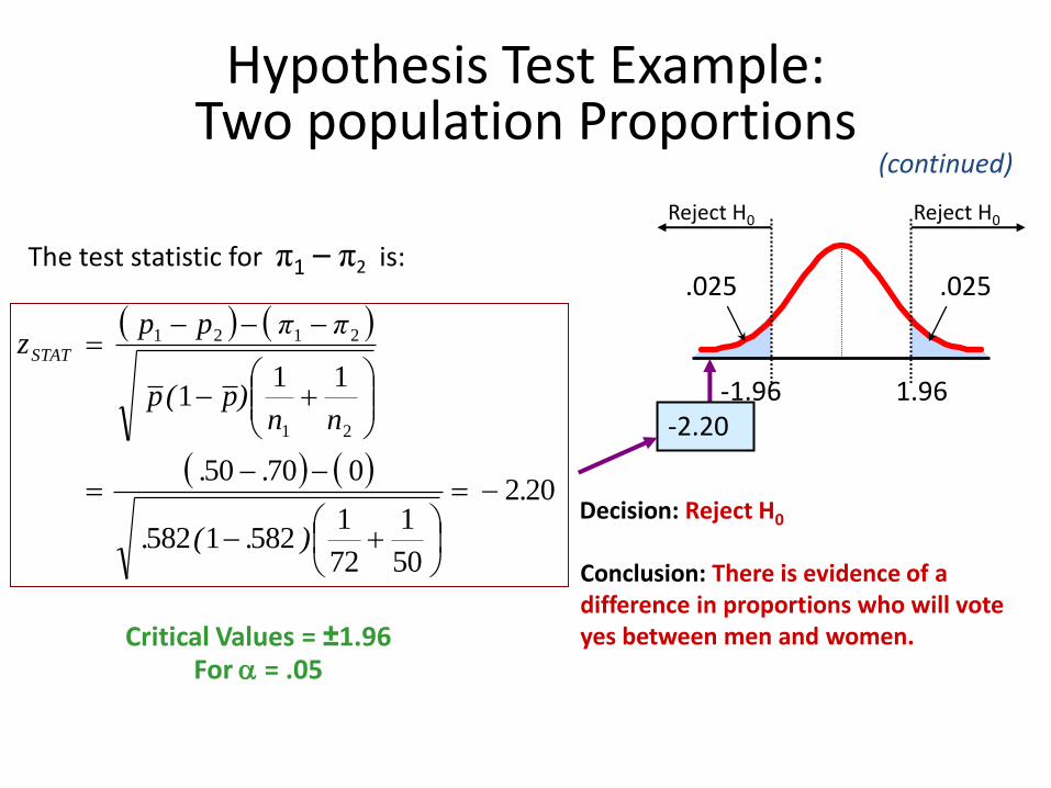
The test statistic for π1 – π2 is:
Hypothesis Test Example: Two population Proportions
(continued)
.025
-1.96 1.96
.025
-2.20
Decision: Reject H0
Conclusion: There is evidence of a difference in proportions who will vote yes between men and women.
202
50
1
72
15821582
07050
111
21
2121
.
).(.
..
nn)p(p
ππppzSTAT
Reject H0 Reject H0
Critical Values = ±1.96 For a = .05

Confidence Interval for Two Population Proportions
2
22
1
11/221
n
)p(1p
n
)p(1pZpp
a
The confidence interval for
π1 – π2 is: Population proportions

Two-Sample Tests
Two-Sample Tests
Population Means
Independent Samples
unknown, assumed
equal
unknown, assumed unequal
Related Samples
Population Proportions
Population Variances
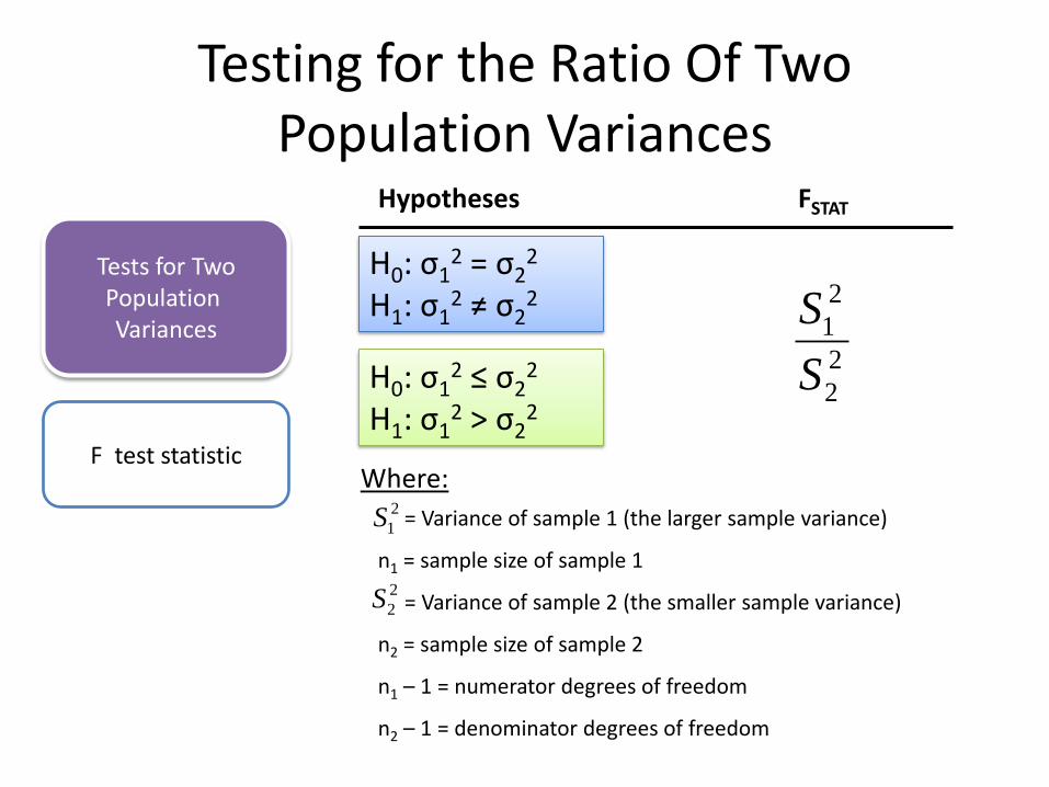
Testing for the Ratio Of Two Population Variances
Tests for Two Population Variances
F test statistic
H0: σ12 = σ2
2 H1: σ1
2 ≠ σ22
H0: σ12 ≤ σ2
2 H1: σ1
2 > σ22
Hypotheses FSTAT
= Variance of sample 1 (the larger sample variance)
n1 = sample size of sample 1
= Variance of sample 2 (the smaller sample variance)
n2 = sample size of sample 2
n1 – 1 = numerator degrees of freedom
n2 – 1 = denominator degrees of freedom
Where: 2
1S
2
2S
2
2
2
1
S
S

• The F critical value is found from the F table
• There are two degrees of freedom required: numerator and denominator
• The larger sample variance is always the numerator
• When
• In the F table,
– numerator degrees of freedom determine the column
– denominator degrees of freedom determine the row
The F Distribution
df1 = n1 – 1 ; df2 = n2 – 1 2
2
2
1
S
SFSTAT

Finding the Rejection Region
H0: σ12 = σ2
2 H1: σ1
2 ≠ σ22
H0: σ12 ≤ σ2
2 H1: σ1
2 > σ22
F 0 a
Fα Reject H0 Do not
reject H0
Reject H0 if FSTAT > Fα
F 0
a/2
Reject H0 Do not reject H0 Fα/2
Reject H0 if FSTAT > Fα/2

F Test: An Example
Anda adalah seorang analis keuangan dan ingin membandingkan hasil dividen antara saham yang terdaftar di NYSE & NASDAQ? Anda mengumpulkan data sebagai berikut:
NYSE NASDAQ Jumlah 21 25 Rata-rata sampel 3.27 2.53 Std dev sampel 1.30 1.16
Apakah terdapat perbedaan
variansi antara hasil dividen pada
NYSE & NASDAQ pada tingkat
signifikansi 0,05?

F Test: Example Solution
• Form the hypothesis test:
(there is no difference between variances)
(there is a difference between variances)
Find the F critical value for a = 0.05:
Numerator d.f. = n1 – 1 = 21 –1 = 20
Denominator d.f. = n2 – 1 = 25 –1 = 24
Fα/2 = F.025, 20, 24 = 2.33
2
2
2
11
2
2
2
10
σ : σH
σ : σH

• The test statistic is:
0
256.116.1
30.12
2
2
2
2
1 S
SFSTAT
a/2 = .025
F0.025=2.33 Reject H0 Do not
reject H0
H0: σ12 = σ2
2 H1: σ1
2 ≠ σ22
F Test: Example Solution
FSTAT = 1.256 is not in the rejection region, so we do not reject H0
(continued)
Conclusion: There is insufficient evidence of a difference in variances at a = .05
F

EXERCISE

10.30 (cont’d)
Apakah tahun ini diperlukan usaha lebih untuk keluar dari sebuah mailing list dari tahun sebelumnya? Sebuah penelitian dari 100 peritel online besar menunjukkan data berikut:
PERLU TIGA ATAU LEBIH KLIK
SEBELUM KELUAR TAHUN Ya Tidak
2009 39 61 2008 7 93

10.30
a. Tentukan hipothesis kosong dan hipothesis alternatif untuk mengetahui apakah diperlukan usaha lebih untuk keluar dari sebuah mailing list jika dibandingkan dengan tahun sebelumnya.
b. Lakukan uji hipothesis untuk poin (a), dengan menggunakan tingkat signifikansi 0,05.
c. Apakah hasil dari poin (b) sesuai dengan klaim bahwa diperlukan usaha lebih untuk keluar dari sebuah mailing list jika dibandingkan dengan tahun sebelumnya?
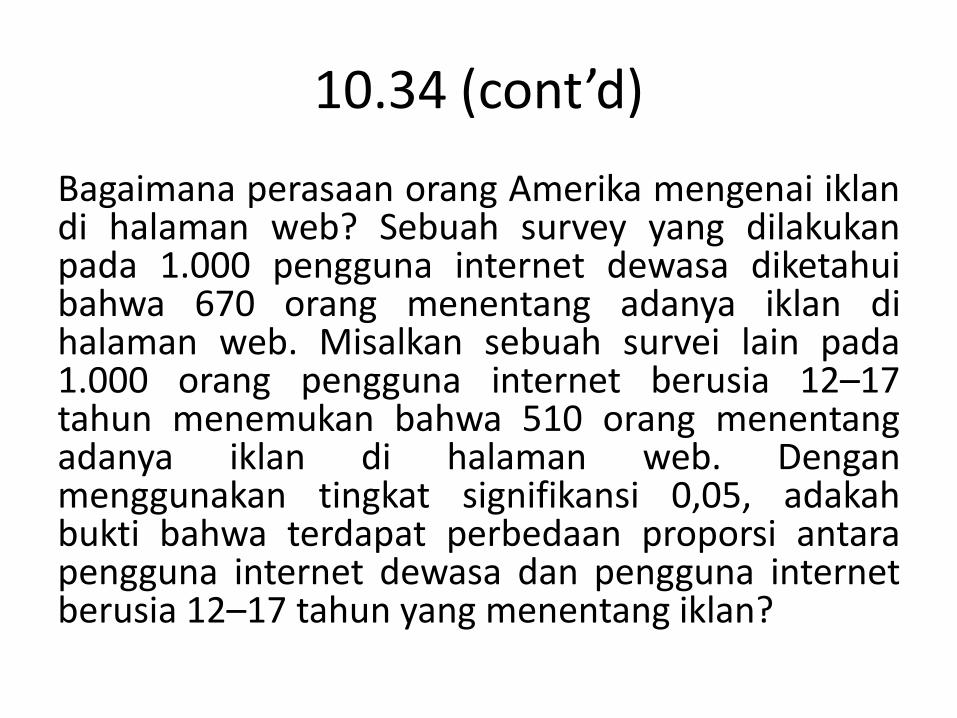
10.34 (cont’d)
Bagaimana perasaan orang Amerika mengenai iklan di halaman web? Sebuah survey yang dilakukan pada 1.000 pengguna internet dewasa diketahui bahwa 670 orang menentang adanya iklan di halaman web. Misalkan sebuah survei lain pada 1.000 orang pengguna internet berusia 12–17 tahun menemukan bahwa 510 orang menentang adanya iklan di halaman web. Dengan menggunakan tingkat signifikansi 0,05, adakah bukti bahwa terdapat perbedaan proporsi antara pengguna internet dewasa dan pengguna internet berusia 12–17 tahun yang menentang iklan?

10.46 (cont’d)
Computer Anxiety Rating Scale (CARS) mengukur tingkat kecemasan terhadap komputer (computer anxiety), dengan skala dari 20 (tidak ada kecemasan) hingga 100 (sangat cemas). Peneliti dari Miami University menyebarjab CARS pada 172 mahasiswa bisnis. Salah satu tujuan dari penelitian tersebut adalah menentukan apakah terdapat perbedaan tingkat kecemasan komputer yang dirasakan oleh mahasiswa bisnis pria dan wanita. Mereka menemukan data berikut:
Pria Wanita X 40.26 36.85 S 13.35 9.42 n 100 72

10.46
a. Dengan tingkat signifikansi 0,05, adakah bukti yang menunjukkan perbedaan sebaran (variability) kecemasan komputer (computer anxiety) yang dialami pria dan wanita?
b. Asumsi apa yang anda perlukan tentang kedua populasi tersebut untuk dapat menggunakan uji F?
c. Berdasarkan poin (a) dan (b), uji t manakah yang seharusnya anda gunakan untuk menguji apakah ada perbedaan yang signifikan antara kecemasan komputer yang dirasakan oleh wanita dan pria?

THANK YOU