STATISTICAL PHYSICS AND ECOLOGY
143
The Pennsylvania State University The Graduate School Department of Physics STATISTICAL PHYSICS AND ECOLOGY A Thesis in Physics by Igor Volkov c 2005 Igor Volkov Submitted in Partial Fulfillment of the Requirements for the Degree of Doctor of Philosophy August 2005
Transcript of STATISTICAL PHYSICS AND ECOLOGY
The Pennsylvania State University
The Graduate School
Department of Physics
STATISTICAL PHYSICS AND ECOLOGY
A Thesis in
Physics
by
Igor Volkov
c© 2005 Igor Volkov
Submitted in Partial Fulfillmentof the Requirements
for the Degree of
Doctor of Philosophy
August 2005

ii
The thesis of Igor Volkov has been reviewed and approved∗ by the following:
Jayanth Banavar
Distinguished Professor and Head of Physics
Thesis Adviser
Chair of Committee
Bryan Grenfell
Alumni Professor of the Biological Sciences
Julian Maynard
Distinguished Professor of Physics
Peter Schiffer
Professor of Physics
∗Signatures are on file in the Graduate School.
iii
Abstract
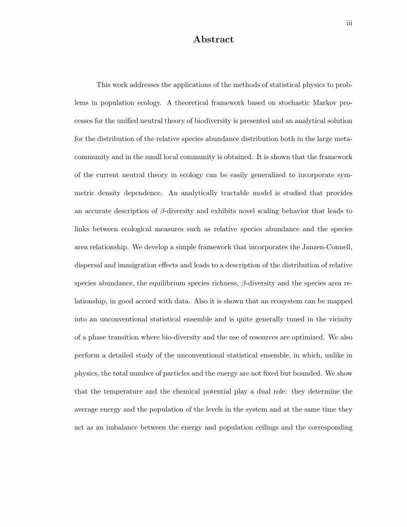
This work addresses the applications of the methods of statistical physics to prob-
lems in population ecology. A theoretical framework based on stochastic Markov pro-
cesses for the unified neutral theory of biodiversity is presented and an analytical solution
for the distribution of the relative species abundance distribution both in the large meta-
community and in the small local community is obtained. It is shown that the framework
of the current neutral theory in ecology can be easily generalized to incorporate sym-
metric density dependence. An analytically tractable model is studied that provides
an accurate description of β-diversity and exhibits novel scaling behavior that leads to
links between ecological measures such as relative species abundance and the species
area relationship. We develop a simple framework that incorporates the Janzen-Connell,
dispersal and immigration effects and leads to a description of the distribution of relative
species abundance, the equilibrium species richness, β-diversity and the species area re-
lationship, in good accord with data. Also it is shown that an ecosystem can be mapped
into an unconventional statistical ensemble and is quite generally tuned in the vicinity
of a phase transition where bio-diversity and the use of resources are optimized. We also
perform a detailed study of the unconventional statistical ensemble, in which, unlike in
physics, the total number of particles and the energy are not fixed but bounded. We show
that the temperature and the chemical potential play a dual role: they determine the
average energy and the population of the levels in the system and at the same time they
act as an imbalance between the energy and population ceilings and the corresponding
iv
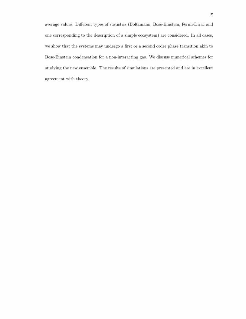
average values. Different types of statistics (Boltzmann, Bose-Einstein, Fermi-Dirac and
one corresponding to the description of a simple ecosystem) are considered. In all cases,
we show that the systems may undergo a first or a second order phase transition akin to
Bose-Einstein condensation for a non-interacting gas. We discuss numerical schemes for
studying the new ensemble. The results of simulations are presented and are in excellent
agreement with theory.
v
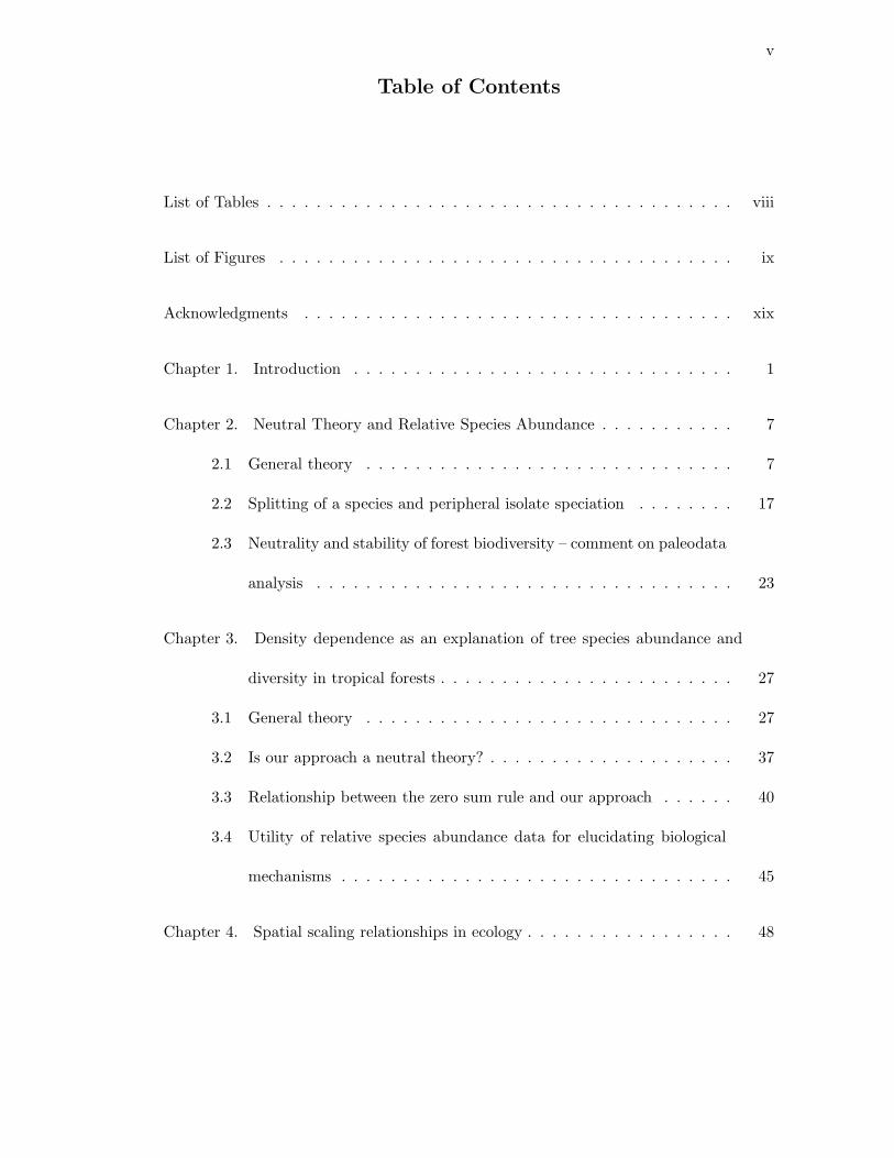
Table of Contents
List of Tables . . . . . . . . . . . . . . . . . . . . . . . . . . . . . . . . . . . . . . viii
List of Figures . . . . . . . . . . . . . . . . . . . . . . . . . . . . . . . . . . . . . ix
Acknowledgments . . . . . . . . . . . . . . . . . . . . . . . . . . . . . . . . . . . xix
Chapter 1. Introduction . . . . . . . . . . . . . . . . . . . . . . . . . . . . . . . 1
Chapter 2. Neutral Theory and Relative Species Abundance . . . . . . . . . . . 7
2.1 General theory . . . . . . . . . . . . . . . . . . . . . . . . . . . . . . 7
2.2 Splitting of a species and peripheral isolate speciation . . . . . . . . 17
2.3 Neutrality and stability of forest biodiversity – comment on paleodata
analysis . . . . . . . . . . . . . . . . . . . . . . . . . . . . . . . . . . 23
Chapter 3. Density dependence as an explanation of tree species abundance and
diversity in tropical forests . . . . . . . . . . . . . . . . . . . . . . . . 27
3.1 General theory . . . . . . . . . . . . . . . . . . . . . . . . . . . . . . 27
3.2 Is our approach a neutral theory? . . . . . . . . . . . . . . . . . . . . 37
3.3 Relationship between the zero sum rule and our approach . . . . . . 40
3.4 Utility of relative species abundance data for elucidating biological
mechanisms . . . . . . . . . . . . . . . . . . . . . . . . . . . . . . . . 45
Chapter 4. Spatial scaling relationships in ecology . . . . . . . . . . . . . . . . . 48
vi
Chapter 5. Spatial patterns of ecological communities: α-β diversity and species-
area relationship . . . . . . . . . . . . . . . . . . . . . . . . . . . . . 58
Chapter 6. Organization of ecosystems in the vicinity of a novel phase transition 71
6.1 Sketch of the derivation . . . . . . . . . . . . . . . . . . . . . . . . . 73
6.2 Results and conclusions . . . . . . . . . . . . . . . . . . . . . . . . . 78
Appendix. A novel ensemble in statistical physics . . . . . . . . . . . . . . . . . 83
A.1 Theoretical framework . . . . . . . . . . . . . . . . . . . . . . . . . . 85
A.2 Theoretical and numerical results for systems with different statistics 94
A.2.1 Boltzmann Statistics (Figures A.1, A.2 and A.3) . . . . . . . 94
A.2.1.1 Theory . . . . . . . . . . . . . . . . . . . . . . . . . 94
A.2.1.2 Simulations . . . . . . . . . . . . . . . . . . . . . . . 95
A.2.2 Fermi-Dirac Statistics (Figures A.4, A.5, A.6 and A.7) . . . . 96
A.2.2.1 Theory . . . . . . . . . . . . . . . . . . . . . . . . . 96
A.2.2.2 Simulations . . . . . . . . . . . . . . . . . . . . . . . 97
A.2.3 Bose-Einstein Statistics (Figures A.8 - A.14) . . . . . . . . . 97
A.2.3.1 Theory . . . . . . . . . . . . . . . . . . . . . . . . . 97
A.2.3.2 Simulations . . . . . . . . . . . . . . . . . . . . . . . 98
A.2.4 Ecological case (Figures A.15 and A.16) . . . . . . . . . . . . 98
A.2.4.1 Theory . . . . . . . . . . . . . . . . . . . . . . . . . 98
A.2.4.2 Simulations . . . . . . . . . . . . . . . . . . . . . . . 99
A.3 Conclusions . . . . . . . . . . . . . . . . . . . . . . . . . . . . . . . . 99

vii
References . . . . . . . . . . . . . . . . . . . . . . . . . . . . . . . . . . . . . . . . 114
viii
List of Tables
3.1 Maximum likelihood estimates of the density-dependant symmetric model
and dispersal limitation model[83] parameters (upper table) and com-
parison between the models (lower table) for the six data sets of tropical
forests. In the six plots coordinated by the Center for Tropical Forest
Science of the Smithsonian (http://www.ctfs.si.edu), we considered trees
with diameter at breast height ≥ 10 cm. S is the number of species, J is
the total abundance and θ1 and θ2 are the biodiversity parameters in the
dispersal limitation model[83] and equation (3.1) respectively (note that
θ2 is a function of c, x and S and both models have the same number of
fitting parameters). The comparison of the models was carried out with
the likelihood ratio test[3, 30, 40]. The lower table presents deviance
(twice the difference in the log-likelihoods L1 and L2) between the two
models and the corresponding P -value of the χ2-distribution with one de-
gree of freedom. The main result is that the dispersal limitation model
and the simple symmetric density dependent model presented here are
statistically comparable to each other in their ability to fit the tropical
forest data. . . . . . . . . . . . . . . . . . . . . . . . . . . . . . . . . . . 34
4.1 Scaling exponents for d = 1, 2, 3 determined from the scaling collapse of
the RSA and SAR plots (Figs. 4.1 and 4.2). . . . . . . . . . . . . . . . 50
ix
List of Figures
2.1 Data on tree species abundances in 50 hectare plot of tropical forest
in Barro Colorado Island, Panama taken from Condit et al.[21]. The
total number of trees in the dataset is 21457 and the number of distinct
species is 225. The red bars are observed numbers of species binned into
log(2) abundance categories, following Preston’s method[75]. The first
histogram bar represents〈φ1〉
2 , the second bar〈φ1〉
2 +〈φ2〉
2 , the third bar
〈φ2〉2 + 〈φ3〉+
〈φ4〉2 , the fourth bar
〈φ4〉2 + 〈φ5〉+ 〈φ6〉+ 〈φ7〉+
〈φ8〉2 and
so on. The black curve shows the best fit to a lognormal distribution
〈φn〉 = Nn exp(− (log2 n−log2 n0)2
2σ2) (N = 46.29, n0 = 20.82 and σ =
2.98), while the green curve is the best fit to our analytic expression
Eq.(2.14) (m = 0.1 from which one obtains θ = 47.226 compared to the
Hubbell[45] estimates of 0.1 and 50 respectively and McGill’s best fits[66]
of 0.079 and 48.5 respectively.) . . . . . . . . . . . . . . . . . . . . . . . 16
2.2 The red bars represent the numbers of species derived from Eq.(2.26)
binned into log(2) abundance categories, following Hubbell’s method[45].
The first histogram bar represents 〈φ1〉, the second bar 〈φ2〉 + 〈φ3〉, the
third bar 〈φ4〉 + 〈φ5〉 + 〈φ6〉 + 〈φ7〉 and so on. Here θ = 40 and p = 40. 22
x
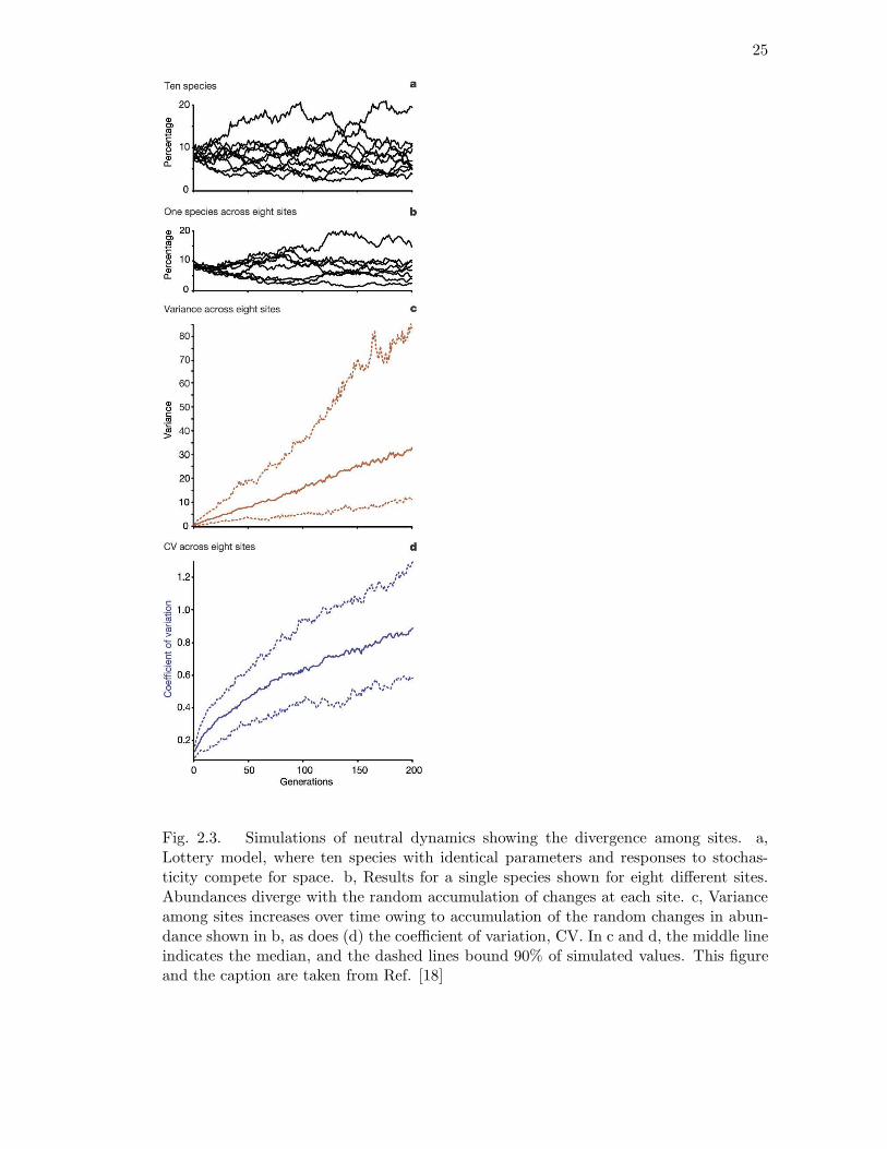
2.3 Simulations of neutral dynamics showing the divergence among sites. a,
Lottery model, where ten species with identical parameters and responses
to stochasticity compete for space. b, Results for a single species shown
for eight different sites. Abundances diverge with the random accumula-
tion of changes at each site. c, Variance among sites increases over time
owing to accumulation of the random changes in abundance shown in
b, as does (d) the coefficient of variation, CV. In c and d, the middle
line indicates the median, and the dashed lines bound 90% of simulated
values. This figure and the caption are taken from Ref. [18] . . . . . . . 25
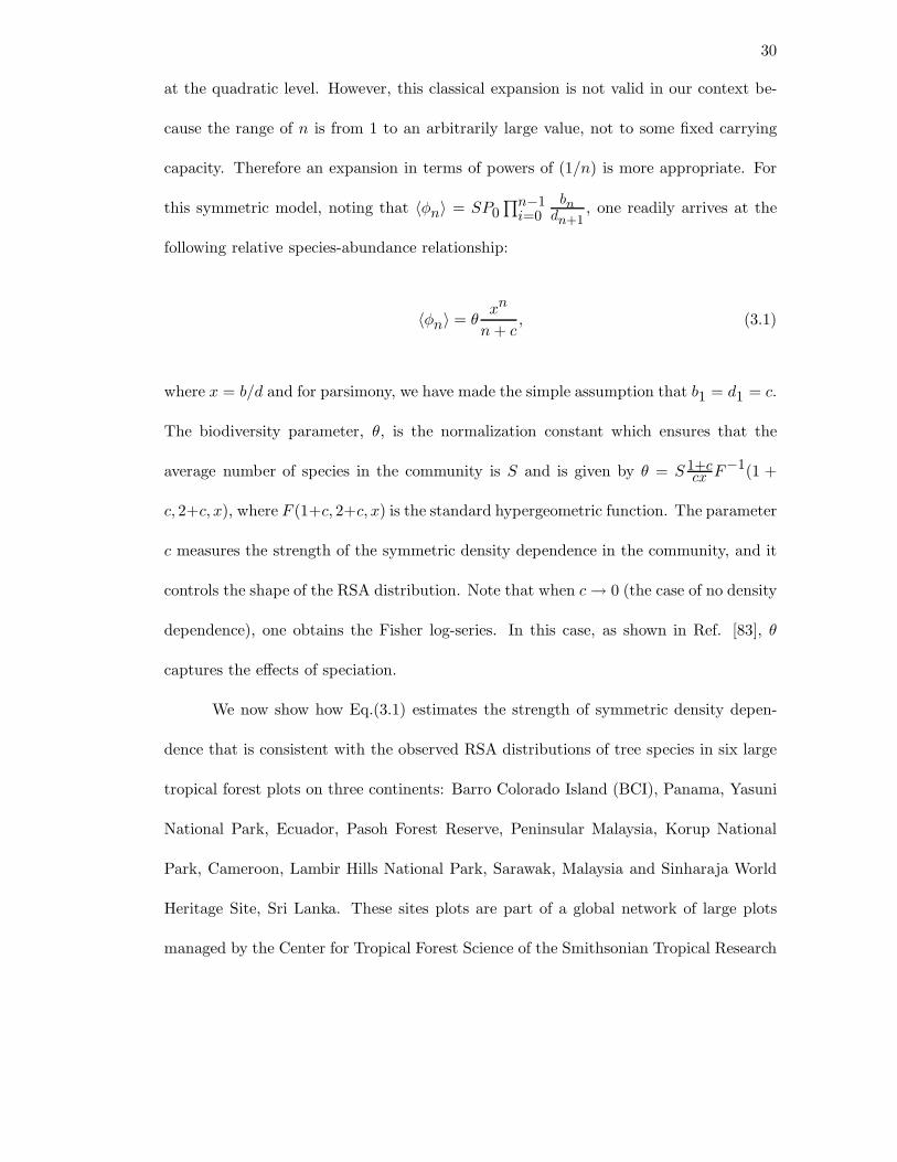
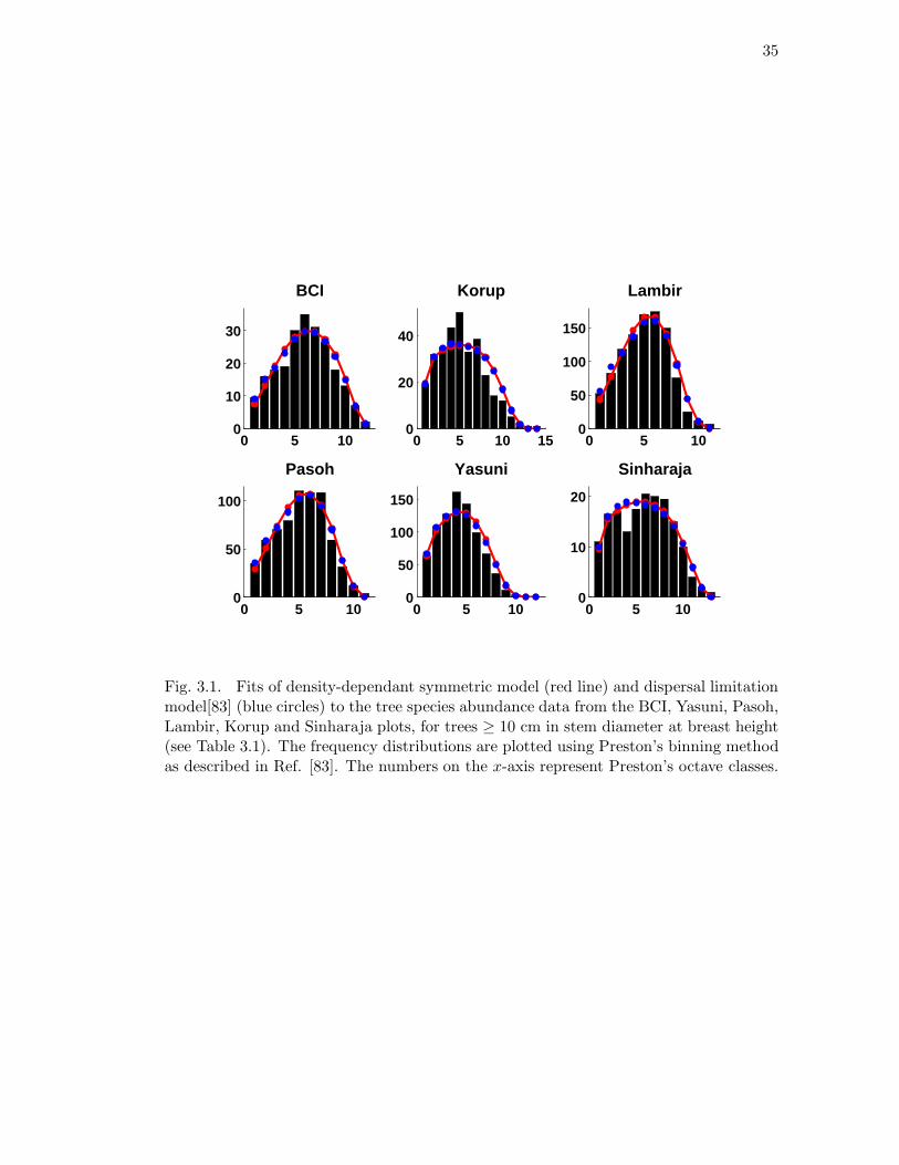
3.1 Fits of density-dependant symmetric model (red line) and dispersal lim-
itation model[83] (blue circles) to the tree species abundance data from
the BCI, Yasuni, Pasoh, Lambir, Korup and Sinharaja plots, for trees
≥ 10 cm in stem diameter at breast height (see Table 3.1). The frequency
distributions are plotted using Preston’s binning method as described in
Ref. [83]. The numbers on the x-axis represent Preston’s octave classes. 35
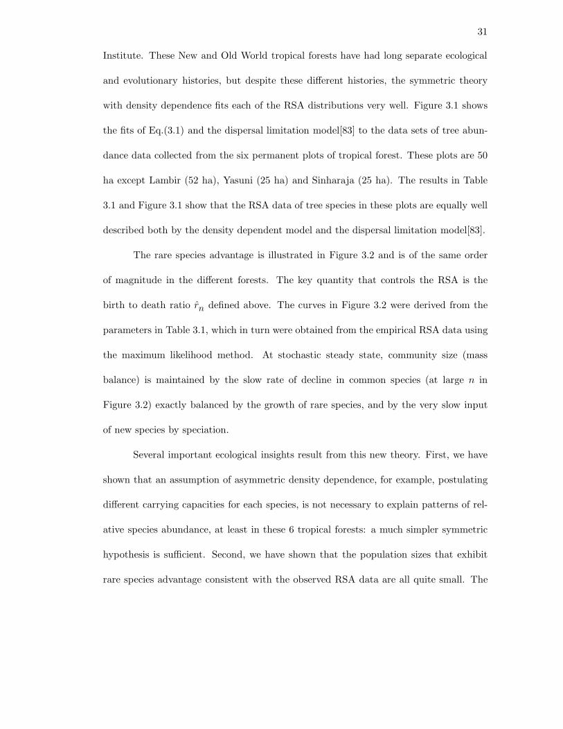
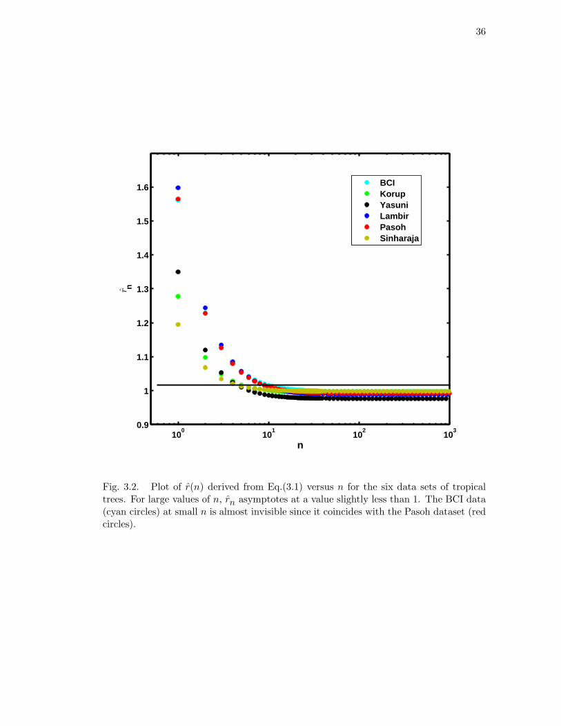
3.2 Plot of r(n) derived from Eq.(3.1) versus n for the six data sets of tropical
trees. For large values of n, rn asymptotes at a value slightly less than
1. The BCI data (cyan circles) at small n is almost invisible since it
coincides with the Pasoh dataset (red circles). . . . . . . . . . . . . . . . 36
xi
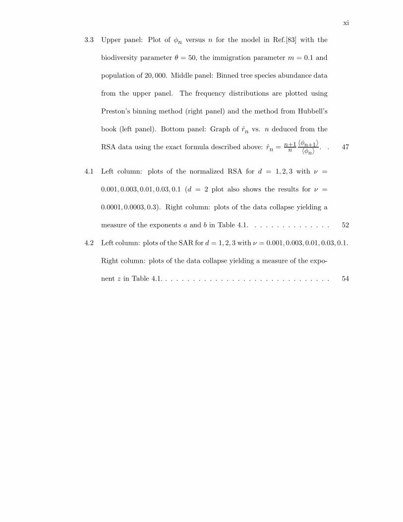
3.3 Upper panel: Plot of φn versus n for the model in Ref.[83] with the
biodiversity parameter θ = 50, the immigration parameter m = 0.1 and
population of 20, 000. Middle panel: Binned tree species abundance data
from the upper panel. The frequency distributions are plotted using
Preston’s binning method (right panel) and the method from Hubbell’s
book (left panel). Bottom panel: Graph of rn vs. n deduced from the
RSA data using the exact formula described above: rn = n+1n
〈φn+1〉〈φn〉
. . 47
4.1 Left column: plots of the normalized RSA for d = 1, 2, 3 with ν =
0.001, 0.003, 0.01, 0.03, 0.1 (d = 2 plot also shows the results for ν =
0.0001, 0.0003, 0.3). Right column: plots of the data collapse yielding a
measure of the exponents a and b in Table 4.1. . . . . . . . . . . . . . . 52
4.2 Left column: plots of the SAR for d = 1, 2, 3 with ν = 0.001, 0.003, 0.01, 0.03, 0.1.
Right column: plots of the data collapse yielding a measure of the expo-
nent z in Table 4.1. . . . . . . . . . . . . . . . . . . . . . . . . . . . . . . 54

xii
5.1 Relative Species Abundance plots for a metacommunity with JM =
11400 individuals. Here 〈φn〉 is the number of species with population n,
S denotes the total number of species, ν is the speciation rate and R is the
Janzen-Connell length scale. The two mean field cases are well-described
by the Fisher log-series (thin blue line fits). The three cases with ν = 0.1
(dashed lines) lead to overlapping plots. The Janzen-Connell effects are
not important in these cases because of the few individuals per species.
For the three cases with ν = 0.005, there is a pronounced internal mode
with the behavior at intermediate values of R being distinct from the
R = 0 and ∞ cases. . . . . . . . . . . . . . . . . . . . . . . . . . . . . . 67
5.2 Beta Diversity data along with the best fits using Equation (1) for plots in
(a) Panama (R = 46m, γ−10
= 68m, γ−11
= 210km and c0 = 120m) and
in (b) Ecuador-Peru (Yasuni) (R = 86m, γ−10
= 69m, γ−11
= 23, 500km
and c0 = 19m). The Janzen-Connell effect pushes conspecific individuals
further away from each other and thus the probability function F declines
more steeply within the zone of its operation than at larger distances as
in the data. . . . . . . . . . . . . . . . . . . . . . . . . . . . . . . . . . . 68
xiii
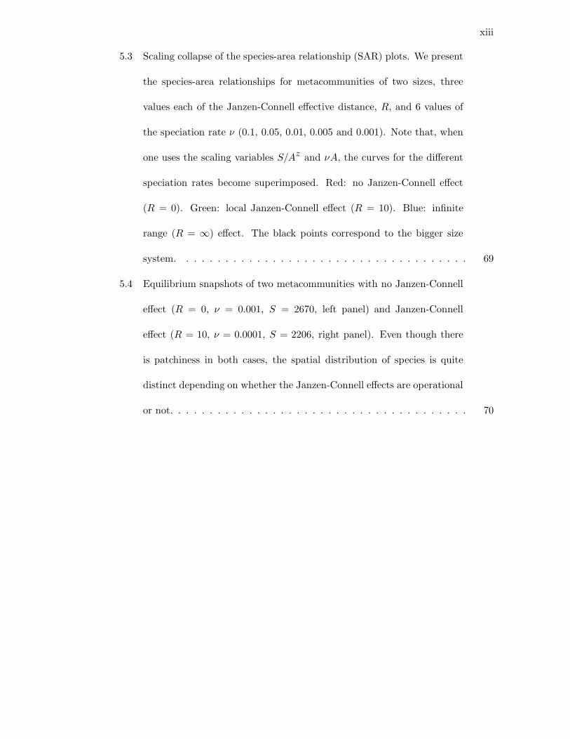
5.3 Scaling collapse of the species-area relationship (SAR) plots. We present
the species-area relationships for metacommunities of two sizes, three
values each of the Janzen-Connell effective distance, R, and 6 values of
the speciation rate ν (0.1, 0.05, 0.01, 0.005 and 0.001). Note that, when
one uses the scaling variables S/Az and νA, the curves for the different
speciation rates become superimposed. Red: no Janzen-Connell effect
(R = 0). Green: local Janzen-Connell effect (R = 10). Blue: infinite
range (R = ∞) effect. The black points correspond to the bigger size
system. . . . . . . . . . . . . . . . . . . . . . . . . . . . . . . . . . . . . 69
5.4 Equilibrium snapshots of two metacommunities with no Janzen-Connell
effect (R = 0, ν = 0.001, S = 2670, left panel) and Janzen-Connell
effect (R = 10, ν = 0.0001, S = 2206, right panel). Even though there
is patchiness in both cases, the spatial distribution of species is quite
distinct depending on whether the Janzen-Connell effects are operational
or not. . . . . . . . . . . . . . . . . . . . . . . . . . . . . . . . . . . . . . 70

xiv
6.1 Comparison of the results of computer simulations of an ecosystem with
theory. We consider a system with 100, 000 energy levels with εk = k2/3,
k = 1..100, 000, corresponding to d = 1/2. We work with a constant
Emax (the figure shows the results for several values of Emax) and con-
sider a dynamical process of birth and death. We have verified that the
equilibrium distribution is independent of the initial condition. At any
given time step, we make a list of all the individuals and the empty
energy levels. One of the entries from the list is randomly picked for
possible action with a probability proportional to the total number of
entries in the list. Were an individual to be picked, it is killed with 50%
probability or reproduced (an additional individual of the same species
is created) with 50% probability provided the total energy of the system
does not exceed Emax. When an empty energy level is picked, specia-
tion occurs with 50% probability and a new individual of that species is
created provided again the energy of the system does not exceed Emax.
With 50% probability, no action is taken. This procedure is iterated un-
til equilibrium is reached. The effective temperature of the ecosystem is
defined as the imbalance between Emax and the average energy of the
system (Eq. (6.1)). The figure shows a plot of the effective temperature
of the ecosystem deduced from the simulations. The circles denote the
data averaged over a run of 109 time steps with the last 500 million used
to compute the average temperature while the solid line is the theoretical
prediction. . . . . . . . . . . . . . . . . . . . . . . . . . . . . . . . . . . . 80
xv
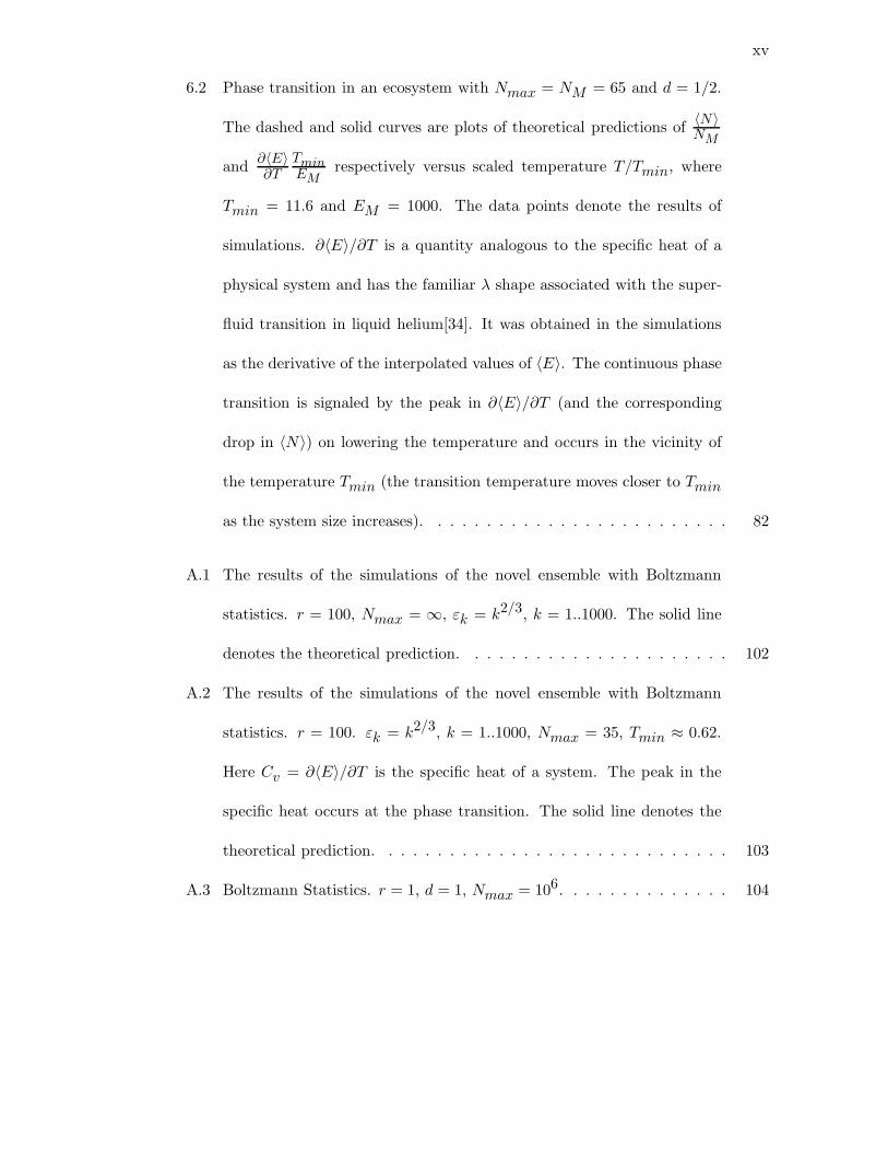
6.2 Phase transition in an ecosystem with Nmax = NM = 65 and d = 1/2.
The dashed and solid curves are plots of theoretical predictions of〈N〉NM
and∂〈E〉∂T
TminEM
respectively versus scaled temperature T/Tmin, where
Tmin = 11.6 and EM = 1000. The data points denote the results of
simulations. ∂〈E〉/∂T is a quantity analogous to the specific heat of a
physical system and has the familiar λ shape associated with the super-
fluid transition in liquid helium[34]. It was obtained in the simulations
as the derivative of the interpolated values of 〈E〉. The continuous phase
transition is signaled by the peak in ∂〈E〉/∂T (and the corresponding
drop in 〈N〉) on lowering the temperature and occurs in the vicinity of
the temperature Tmin (the transition temperature moves closer to Tmin
as the system size increases). . . . . . . . . . . . . . . . . . . . . . . . . 82
A.1 The results of the simulations of the novel ensemble with Boltzmann
statistics. r = 100, Nmax = ∞, εk = k2/3, k = 1..1000. The solid line
denotes the theoretical prediction. . . . . . . . . . . . . . . . . . . . . . 102
A.2 The results of the simulations of the novel ensemble with Boltzmann
statistics. r = 100. εk = k2/3, k = 1..1000, Nmax = 35, Tmin ≈ 0.62.
Here Cv = ∂〈E〉/∂T is the specific heat of a system. The peak in the
specific heat occurs at the phase transition. The solid line denotes the
theoretical prediction. . . . . . . . . . . . . . . . . . . . . . . . . . . . . 103
A.3 Boltzmann Statistics. r = 1, d = 1, Nmax = 106. . . . . . . . . . . . . . 104
xvi
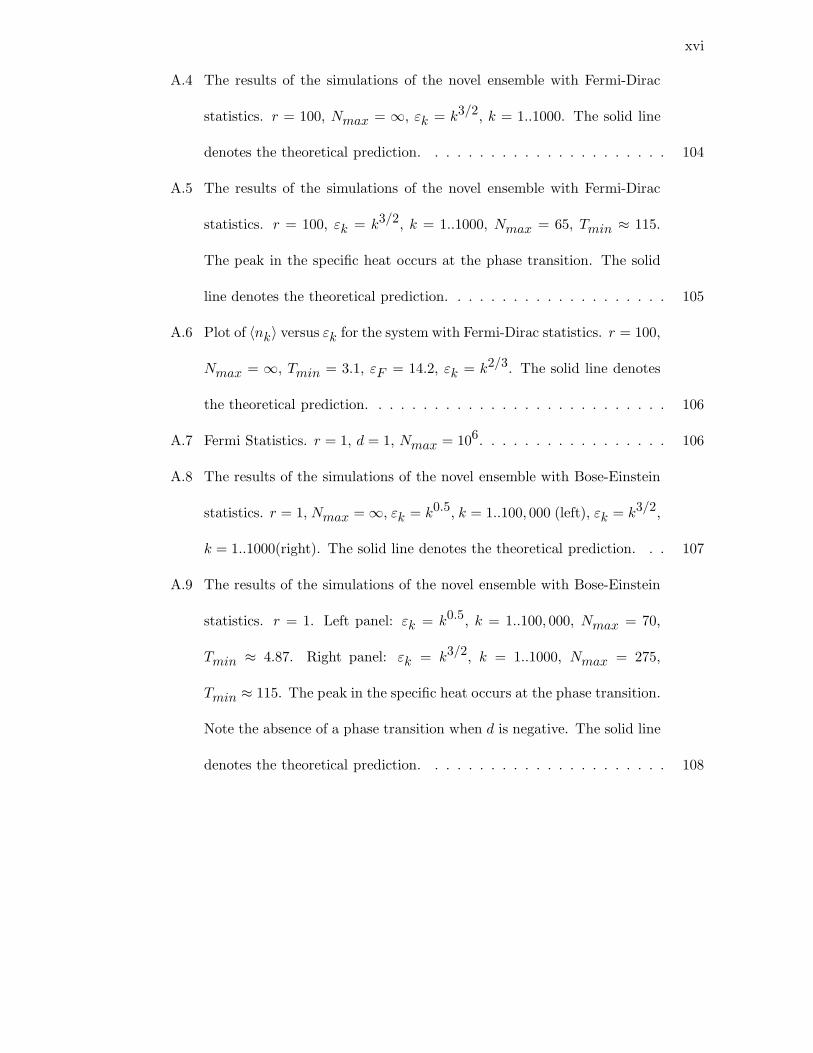
A.4 The results of the simulations of the novel ensemble with Fermi-Dirac
statistics. r = 100, Nmax = ∞, εk = k3/2, k = 1..1000. The solid line
denotes the theoretical prediction. . . . . . . . . . . . . . . . . . . . . . 104
A.5 The results of the simulations of the novel ensemble with Fermi-Dirac
statistics. r = 100, εk = k3/2, k = 1..1000, Nmax = 65, Tmin ≈ 115.
The peak in the specific heat occurs at the phase transition. The solid
line denotes the theoretical prediction. . . . . . . . . . . . . . . . . . . . 105
A.6 Plot of 〈nk〉 versus εk for the system with Fermi-Dirac statistics. r = 100,
Nmax = ∞, Tmin = 3.1, εF = 14.2, εk = k2/3. The solid line denotes
the theoretical prediction. . . . . . . . . . . . . . . . . . . . . . . . . . . 106
A.7 Fermi Statistics. r = 1, d = 1, Nmax = 106. . . . . . . . . . . . . . . . . 106
A.8 The results of the simulations of the novel ensemble with Bose-Einstein
statistics. r = 1, Nmax = ∞, εk = k0.5, k = 1..100, 000 (left), εk = k3/2,
k = 1..1000(right). The solid line denotes the theoretical prediction. . . 107
A.9 The results of the simulations of the novel ensemble with Bose-Einstein
statistics. r = 1. Left panel: εk = k0.5, k = 1..100, 000, Nmax = 70,
Tmin ≈ 4.87. Right panel: εk = k3/2, k = 1..1000, Nmax = 275,
Tmin ≈ 115. The peak in the specific heat occurs at the phase transition.
Note the absence of a phase transition when d is negative. The solid line
denotes the theoretical prediction. . . . . . . . . . . . . . . . . . . . . . 108
xvii
A.10 The results of the simulations of the novel ensemble with Bose-Einstein
statistics. r = 0.33/0.67. Nmax = ∞. Left panel: εk = k3/2, k =
1..1000. Right panel : εk = k2/3, k = 1..10000. The solid line denotes
the theoretical prediction. . . . . . . . . . . . . . . . . . . . . . . . . . . 109
A.11 The results of the simulations of the novel ensemble with Bose-Einstein
statistics. r = 0.33/0.67. Left panel: Nmax = 45, εk = k3/2, k =
1..1000, Tmin ≈ 545. Right panel: Nmax = 16, εk = k2/3, k = 1..10000,
Tmin ≈ 7.5. . . . . . . . . . . . . . . . . . . . . . . . . . . . . . . . . . . 110
A.12 The results of the simulations of the novel ensemble with Bose-Einstein
statistics. r = 0.67/0.33, Nmax = ∞, εk = k2/3, k = 1..1000. Solid
lines and circles represent theory and simulations, respectively. Note
the deviation from the theory as the system approaches the “infinite”
temperature ε1/ ln(r). The solid line denotes the theoretical prediction. 111
A.13 The results of the simulations of the novel ensemble with Bose-Einstein
statistics. r = 0.67/0.33, Nmax = 50, εk = k2/3, k = 1..1000 . . . . . . 111
A.14 Bose Statistics. r = 1, d = 1, Nmax = 106. . . . . . . . . . . . . . . . . 112
A.15 The results of the simulations of the model of an ecosystem with r = 1,
Nmax = ∞. Left panel: εk = k3/2, k = 1..1000. Right panel : εk =
k2/3, k = 1..1000. The solid line denotes the theoretical prediction. . . . 112

xviii
A.16 The results of the simulations of the model of an ecosystem with r = 1.
Left panel: Nmax = 200, εk = k3/2, k = 1..1000, Tmin ≈ 400. Right
panel: Nmax = 10, εk = k2/3, k = 1..1000, Tmin ≈ 3.6. The peak in
the specific heat occurs at the phase transition. Note that the similarity
between this figure and Fig. A.9 for Bose-Einstein statistics. . . . . . . . 113

xix
Acknowledgments
I am deeply indebted to my adviser, Prof. Jayanth Banavar, for his continuous
support, kind advice and patient guidance through my graduate career. I also would like
to thank Prof. Amos Maritan for his invaluable help and collaboration. I am grateful to
Marek Cieplak, Steve Hubbell and Tommaso Zillio for all their input and collaboration.
I also wish to thank the members of my thesis committee for their encouraging and
valuable comments on my dissertation. I would like to express my sincere gratitude to
Prof. Serguei Zavtrak for his tremendous help during my studies at the Belarus State
University. Finally, this work would be impossible without the support and help of Oleg,
Tanya and significant others.
1
Chapter 1
Introduction
An ecological community represents a formidable many-body problem – one has
an interacting many body system with imperfectly known interactions and a wide range
of spatial and temporal scales. In tropical forests across the globe, ecologists recently
have been able to measure certain quantities such as the distribution of relative species
abundance (RSA), the species area relationship (SAR), and the probability that two
individuals drawn randomly from forests a specified distance apart belong to the same
species (also called β-diversity). In order to make theoretical progress toward under-
standing the relationships among these measures, it is useful to compare the data with
the predictions of tractable models which begin to capture some of the features that are
known to be important in tropical forest tree communities. The performance of the the-
ory confronted by the data should help guide the development of more realistic models
of communities and the processes that assemble them.
A traditional way of describing an ecological community is to assume that the
species differ one from each other in their response to the available resources and in-
teractions with other species. Such differences (known as niches) lead to the situation
where each species is specialized in utilizing it’s partition of the resources and has a
unique role in the functioning of the ecosystem. The total number of species in a par-
ticular ecosystem which defines the biodiversity is thus determined by the variety of the
2
available resources and the ways the species can utilize them. The mathematical models
that seek to capture the niche structure of the ecosystems are, therefore, very complex
and need to rely on a lot of empirical assumptions.
Recently, it has been suggested that niche approach may not be adequate for the
description of the particular ecological communities. For example, there are hundreds
of tree species in the tropical forests that coexist in the environment with a very few
available resources (sun energy, water, soil). It is argued that such a systems cannot
have enough niches to accommodate such a large number of species.
An alternative approach to the description of the community structure, which
is called neutral theory, has been recently proposed by Hubbell[45]. In this model the
population dynamics of the ecosystem is purely stochastic and there are no differences
between species, so that each individual in an ecosystem, regardless of the species it
belongs to, has the same chances of giving birth or dying. Hence, there are no direct
interactions between the species – all the interactions arise from the limited size of the
community. In the neutral model, the species diversity is maintained by the processes of
speciation, when a completely new species emerges.
Unlike niche theory, neutral models use a very small number of inputs, such as the
birth and death rates, and allow for an elegant mathematical formulation of the problem
in the form of a stochastic master equation for a one-step Markov process[82]. Since all
the species are equivalent, one can consider a mean field approach, where a single species
is treated against the backdrop of the others. While neutral theory is controversial in
ecology, such approaches have been employed in physics for a long time. Indeed, one
can draw analogies between the “neutral” treatment of individuals in the ecosystem and
3
the concept of the ideal gas in physics, where the interactions between the particles are
neglected. Similar to the ideal gas, neutral theory can serve as a “null” model for studies
of ecosystems. Starting with the neutral framework one can begin to incorporate the
differences and interactions among species thus finally approaching niche theory. In this
thesis we demonstrate how the neutral model, with very simple modifications, can be
used successfully in the analysis of community patterns.
We begin with the study of the theory of island biogeography[63] which asserts
that an island or a local community approaches an equilibrium species richness as a
result of the interplay between the immigration of species from the much larger meta-
community source area and local extinction of species on the island (local community).
Hubbell[45] generalized this neutral theory to explore the expected steady-state distri-
bution of relative species abundance (RSA) in the local community under restricted
immigration. In Chapter 2 we present a theoretical framework for the unified neutral
theory of biodiversity[45] and an analytical solution for the distribution of the RSA both
in the metacommunity (Fisher’s logseries) and in the local community, where there are
fewer rare species. Rare species are more extinction-prone, and once they go locally
extinct, they take longer to re-immigrate than do common species. Contrary to recent
assertions[66], we show that the analytical solution provides a better fit, with fewer free
parameters, to the RSA distribution of tree species on Barro Colorado Island (BCI)[21]
than the lognormal distribution[75, 65].
Explaining recurrent patterns in the commonness and rarity of species in ecolog-
ical communities has been a central goal of community ecology for more than half a
century[35, 75]. In Chapter 3 we show that the framework of the current neutral theory
4
in ecology[83, 45, 7, 67, 8, 81, 42, 3] can be easily generalized to incorporate symmetric
density dependence[51, 22, 17, 16]. One can calculate precisely the strength of the rare
species advantage that is needed for an explanation of a given RSA distribution. In
Chapter 2 we demonstrated that a mechanism of dispersal limitation also fits RSA data
well[83, 45]. Here we compare fits of the dispersal and density dependence mechanisms
for the empirical RSA data on tree species in six New and Old World tropical forests and
demonstrate that both mechanisms offer sufficient and independent explanations. We
suggest that RSA data by themselves cannot be used to discriminate among these expla-
nations of RSA patterns[31] – empirical studies will be required to determine whether
RSA patterns are due to one or the other mechanism, or to some combination of both.
Another major scientific challenge is to explain the very high levels of tree di-
versity in many tropical forests. One aspect of this challenge is to understand the
evolutionary origin and maintenance of this diversity on large spatial and temporal
scales[69]. Another is to understand how such extraordinarily high tree diversity can
be maintained on very local scales in some tropical forests. For example, there are over
a thousand tree species in a 52 ha plot in Borneo (Lambir, Sarawak). Numerous mech-
anisms have been proposed to explain tropical tree species coexistence on local scales;
many of these hypotheses invoke density- and frequency dependent mechanisms. Two
of the most prominent of these hypotheses are the Janzen-Connell hypothesis[51, 22]
and the Chesson-Warner hypothesis[17]. The Janzen-Connell hypothesis is that seeds
that disperse farther away from the maternal parent are more likely to escape mortality
from host-specific predators or pathogens. This spatially structured mortality disfa-
vors the population growth of locally abundant species relative to uncommon species

5
by reducing the probability of species’ self-replacement in the same location in the
next generation. The Chesson-Warner hypothesis is that a rare-species reproductive
advantage arises when species have similar per capita rates of mortality but reproduce
asynchronously, and there are overlapping generations. Processes that hold the abun-
dance of a common species in check inevitably lead to rare species advantage because
the space or resources freed up by density-dependent deaths are then exploited by less
common species. Therefore, among-species frequency dependence is the community level
consequence of within-species density dependence, and thus they are two different mani-
festations of the same phenomenon. There is accumulating empirical evidence that such
density- and frequency dependent processes may play a large role in maintaining the
diversity of tropical tree communities[5, 47, 37, 20, 38, 89].
In Chapter 4 we present an analytically tractable model that provides an accurate
description of β-diversity and exhibits novel scaling behavior that leads to links between
ecological measures such as relative species abundance and the species area relationship.
A simple framework presented in Chapter 5, incorporates the Janzen-Connell,
dispersal and immigration effects and leads to a description of the distribution of relative
species abundance, the equilibrium species richness, β diversity and the species area
relationship, in good accord with data.
An ecological community consists of individuals of different species occupying
a confined territory and sharing its resources[63, 65, 60, 88]. One may draw parallels
between such a community and a physical system consisting of particles. One of the
most marvelous phenomena in physics is Bose-Einstein condensation[10, 27, 28] (BEC)
in which a system of a conserved number of indistinguishable particles, on cooling to very

6
low temperatures, abruptly occupies the lowest possible energy state. BEC is related to
superfluidity[53, 71] and superconductivity[52, 6] and has been observed in dilute gases
of alkali atoms[4, 23]. In Chapter 6 we show that an ecosystem can be mapped into
an unconventional statistical ensemble and is quite generally tuned in the vicinity of a
phase transition where bio-diversity and the use of resources are optimized. Strikingly
this transition is analogous to BEC but in a classical context.
In the Appendix we present a detailed derivation of the unconventional statistical
ensemble, in which, unlike in physics, the total number of particles and the energy
are not fixed but bounded. We show that the temperature and the chemical potential
play a dual role: they determine the average energy and the population of the levels
in the system and at the same time they act as an imbalance between the energy and
population ceilings and the corresponding average values. Different types of statistics
(Boltzmann, Bose-Einstein, Fermi-Dirac and one corresponding to the description of a
simple ecosystem) are considered. In all cases, we show that the systems may undergo
a first or a second order phase transition akin to Bose-Einstein condensation for a non-
interacting gas. We discuss numerical schemes for studying the new ensemble. The
results of simulations are presented and are in excellent agreement with theory.
7
Chapter 2
Neutral Theory and Relative Species Abundance
2.1 General theory
The neutral theory in ecology[45, 8] seeks to capture the influence of speciation,
extinction, dispersal, and ecological drift on the RSA under the assumption that all
species are demographically alike on a per capita basis. This assumption, while only
an approximation[24, 80, 86], appears to provide a useful description of an ecological
community on some spatial and temporal scales[45, 8]. More significantly, it allows
the development of a tractable null theory for testing hypotheses about community
assembly rules. However, until now, there has been no analytical derivation of the
expected equilibrium distribution of RSA in the local community, and fits to the theory
have required simulations[45] with associated problems of convergence times, unspecified
stopping rules, and precision[66].
The dynamics of the population of a given species is governed by generalized birth
and death events (including speciation, immigration and emigration). Let bn,k and dn,k
represent the probabilities of birth and death, respectively, in the k-th species with n
individuals with b−1,k = d0,k = 0. Let pn,k(t) denote the probability that the k-th
species contains n individuals at time t. In the simplest scenario, the time evolution of
8
pn,k(t) is regulated by the master equation[11, 13, 33]:
dpn,k(t)
dt= pn+1,k(t)dn+1,k + pn−1,k(t)bn−1,k − pn,k(t)(bn,k + dn,k) (2.1)
which leads to the steady-state or equilibrium solution, denoted by P :
Pn,k = P0,k
n−1∏
i=0
bi,k
di+1,k, (2.2)
for n > 0 and where P0,k can be deduced from the normalization condition∑
n Pn,k = 1.
Note that there is no requirement of conservation of community size. One can show
that the system is guaranteed to reach the stationary solution (2.2) in the infinite time
limit[82].
The frequency of species containing n individuals is given by
φn =S∑
k=1
Ik, (2.3)
where S is the total number of species and the indicator Ik is a random variable which
takes the value 1 with probability Pn,k and 0 with probability (1 − Pn,k). Thus the
average number of species containing n individuals is given by
〈φn〉 =S∑
k=1
Pn,k . (2.4)
The RSA relationship we seek to derive is the dependence of 〈φn〉 on n.
9
Let a community consist of species with bn,k ≡ bn and dn,k ≡ dn being indepen-
dent of k (the species are assumed to be demographically identical). From Eq.(2.4), it
follows that 〈φn〉 is simply proportional to Pn, leading to
〈φn〉 = SP0
n−1∏
i=0
bidi+1
. (2.5)
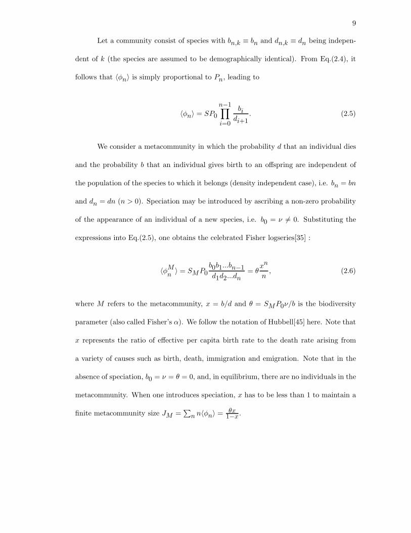
We consider a metacommunity in which the probability d that an individual dies
and the probability b that an individual gives birth to an offspring are independent of
the population of the species to which it belongs (density independent case), i.e. bn = bn
and dn = dn (n > 0). Speciation may be introduced by ascribing a non-zero probability
of the appearance of an individual of a new species, i.e. b0 = ν 6= 0. Substituting the
expressions into Eq.(2.5), one obtains the celebrated Fisher logseries[35] :
〈φMn
〉 = SMP0b0b1...bn−1
d1d2...dn= θ
xn
n, (2.6)
where M refers to the metacommunity, x = b/d and θ = SMP0ν/b is the biodiversity
parameter (also called Fisher’s α). We follow the notation of Hubbell[45] here. Note that
x represents the ratio of effective per capita birth rate to the death rate arising from
a variety of causes such as birth, death, immigration and emigration. Note that in the
absence of speciation, b0 = ν = θ = 0, and, in equilibrium, there are no individuals in the
metacommunity. When one introduces speciation, x has to be less than 1 to maintain a
finite metacommunity size JM =∑
n n〈φn〉 = θx1−x .

10
We turn now to the case of a local community of size J undergoing births and
deaths accompanied by a steady immigration of individuals from the surrounding meta-
community. When the local community is semi-isolated from the metacommunity, one
may introduce an immigration rate m, which is the probability of immigration from the
metacommunity to the local community. For constant m (independent of species), im-
migrants belonging to the more abundant species in the metacommunity will arrive in
the local community more frequently than those of rarer species.
We study the dynamics within a local community following the mathematical
framework of McKane et al.[67], who studied a mean-field stochastic model for species-
rich assembled communities. In our context, the dynamical rules[45] governing the
stochastic processes in the community are:
1) With probability 1 − m, pick two individuals at random from the local com-
munity. If they belong to the same species, no action is taken. Otherwise, with equal
probability, replace one of the individuals with the offspring of the other. In other words,
the two individuals serve as candidates for death and parenthood.
2) With probability m, pick one individual at random from the local community.
Replace it by a new individual chosen with a probability proportional to the abundance of
its species in the metacommunity. This corresponds to the death of the chosen individual
in the local community followed by the arrival of an immigrant from the metacommunity.
Note that the sole mechanism for replenishing species in the local community is immigra-
tion from the metacommunity, which for the purposes of local community dynamics is
treated as a permanent source pool of species, as in the theory of island biogeography[63].

11
These rules are encapsulated in the following expressions for effective birth and
death rates for the k-th species:
bn,k = (1 − m)n
J
J − n
J − 1+ m
µkJM
(1 − n
J
), (2.7)
dn,k = (1 − m)n
J
J − n
J − 1+ m
(1 − µk
JM
)n
J, (2.8)
where µk is the abundance of the k-th species in the metacommunity and JM is the
total population of the metacommunity.
The right hand side of Eq.(2.7) consists of two terms. The first corresponds
to Rule (1) with a birth in the k-th species accompanied by a death elsewhere in the
local community. The second term accounts for an increase of the population of the k-
th species due to immigration from the metacommunity. The immigration is, of course,
proportional to the relative abundance µk/JM of the k-th species in the metacommunity.
Eq.(2.8) follows in a similar manner. Note that bn,k and dn,k not only depend on the
species label k but also are no longer simply proportional to n.
Substituting Eq.(2.7) and Eq.(2.8) into Eq.(2.2), one obtains the expression[67]
Pn,k =J !
n!(J − n)!
Γ(n + λk)
Γ(λk)
Γ(ϑk − n)
Γ(ϑk − J)
Γ(λk + ϑk − J)
Γ(λk + ϑk)≡ F (µk), (2.9)
where
λk =m
(1 − m)(J − 1)
µkJM
(2.10)
12
and
ϑk = J +m
(1 − m)(J − 1)
(1 − µk
JM
). (2.11)
Note that the k dependance in Eq.(2.9) enters only through µk. On substituting
Eq.(2.9) into Eq.(2.4), one obtains
〈φn〉 =
SM∑
k=1
F (µk) = SM 〈F (µk)〉 = SM
∫dµρ(µ)F (µ). (2.12)
Here ρ(µ)dµ is the probability distribution of the mean populations of the species in the
metacommunity and has the form of the familiar Fisher logseries (in a singularity-free
description[35, 76])
ρ(µ)dµ =1
Γ(ε)δε exp(−µ/δ)µε−1
dµ, (2.13)
where δ = x1−x . Substituting Eq.(2.13) into the integral in Eq.(2.12), taking the limits
SM → ∞ and ε → 0 with θ = SM ε approaching a finite value[35, 76] and on defining
y = µ γδθ , one obtains our central result, which is an analytic expression for the RSA of
the local community:
〈φn〉 = θJ !
n!(J − n)!
Γ(γ)
Γ(J + γ)
∫ γ
0
Γ(n + y)
Γ(1 + y)
Γ(J − n + γ − y)
Γ(γ − y)exp(−yθ/γ)dy, (2.14)
where Γ(z) =∫∞0
tz−1e−tdt which is equal to (z − 1)! for integer z and γ =m(J−1)
1−m .
As expected, 〈φn〉 is zero when n exceeds J . The computer calculations in Hubbell’s
book[45] as well as those more recently carried out by McGill[66] were aimed at estimating
〈φn〉 by simulating the processes of birth, death and immigration.

13
One can evaluate the integral in Eq.(2.14) numerically for a given set of parame-
ters: J , θ and m. For large values of n, the integral can be evaluated very accurately and
efficiently using the method of steepest descent[70]. Any given RSA data set contains
information about the local community size, J , and the total number of species in the
local community, SL =∑J
k=1〈φk〉. Thus there is just one free fitting parameter at one’s
disposal.
McGill asserted[66] that the lognormal distribution is a “more parsimonious” null
hypothesis than the neutral theory, a suggestion which is not borne out by our reanalysis
of the BCI data. We focus only on the BCI data set because, as pointed out by McGill[66],
the North American Breeding Bird Survey data are not as exhaustively sampled as the
BCI data set, resulting in fewer individuals and species in any given year in a given
location. Furthermore, McGills analysis seems to rely on adding the bird counts of 5
years at the same sampling locations even though these data sets are not independent.
Figure 2.1 shows a Preston-like binning[75] of the BCI data[21] and the fit of
our analytic expression with one free parameter (11 degrees of freedom) along with a
lognormal having three free parameters (9 degrees of freedom). Standard chi-square
analysis[74] yields values of χ2 = 3.20 for the neutral theory and 3.89 for the lognormal.
The probabilities of such good agreement arising by chance are 1.23% and 8.14% for
the neutral theory and lognormal fits, respectively. Thus one obtains a better fit of the
data with the analytical solution to the neutral theory to BCI than with the lognormal,
even though there are two fewer free parameters. McGill’s analysis[66] on the BCI
data set was based on computer simulations in which there were difficulties in knowing
when to stop the simulations, i.e. when equilibrium had been reached. It is unclear
14
whether McGill averaged over an ensemble of runs, which is essential to obtain repeatable
and reliable results from simulations of stochastic processes because of their inherent
noisiness. However, simulations of the neutral theory are no longer necessary, and all
problems with simulations are moot, because an analytical solution is now available.
The lognormal distribution is biologically less informative and mathematically less
acceptable as a dynamical null hypothesis for the distribution of RSA than the neutral
theory. The parameters of the neutral theory or RSA are directly interpretable in terms
of birth and death rates, immigration rates, size of the metacommunity, and speciation
rates. A dynamical model of a community cannot yield a lognormal distribution with
finite variance because in its time evolution, the variance increases through time without
bound. However, as shown by Sugihara et al.[79], the lognormal distribution can arise
in static models, such as those based on niche hierarchy.
The steady-state deficit in the number of rare species compared to that expected
under the logseries can also occur because rare species grow differentially faster than
common species and therefore move up and out of the rarest abundance categories due
to their rare species advantage[15]. Indeed, it is likely that several different models (e.g.
an empirical lognormal distribution, niche hierarchy models[79] or the theory presented
here) might provide comparable fits to the RSA data (we have found that the lognormal
does slightly better than the neutral theory for the Pasoh data set[64], a tropical tree
community in Malaysia). Such fitting exercises in and of themselves, however, do not
constitute an adequate test of the underlying theory. Neutral theory predicts that the
degree of skewing of the RSA distribution ought to increase as the rate of immigration
into the local community decreases. Dynamic data on rates of birth, death, dispersal and

15
immigration are needed to evaluate the assumptions of neutral theory and determine the
role played by niche differentiation in the assembly of ecological communities.
Our analysis should also apply to the field of population genetics in which the
mutation-extinction equilibrium of neutral allele frequencies at a given locus has been
studied for several decades [55, 32, 54, 85, 57, 56].
16
1 2 4 8 16 32 64 128 256 512 1024 20480
5
10
15
20
25
30
35
BCI Plot
Number of individuals (log2 scale)
Num
ber
of s
peci
es
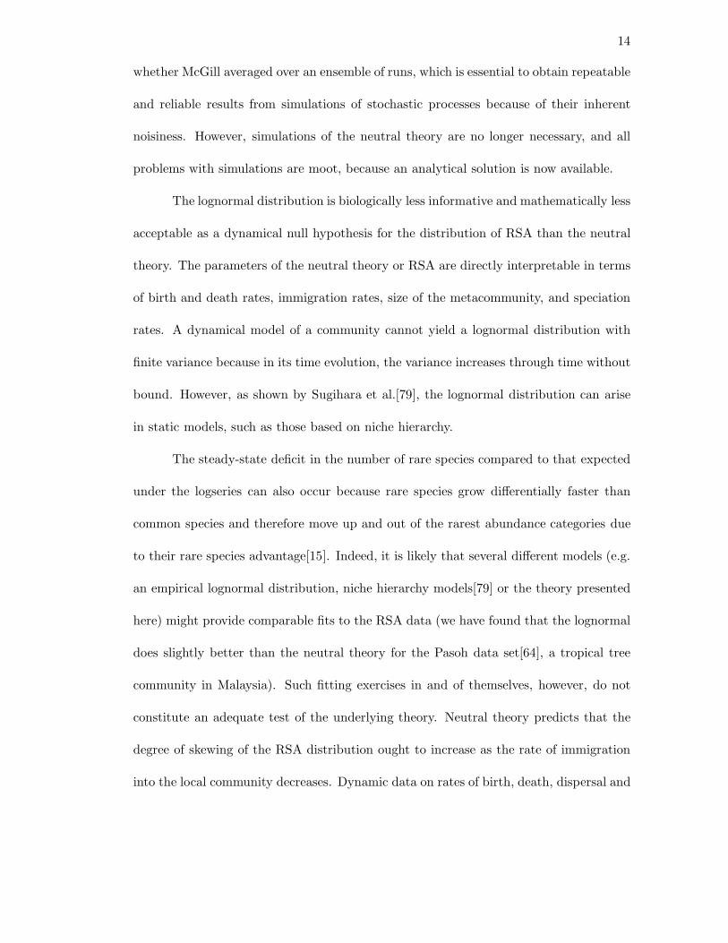
Fig. 2.1. Data on tree species abundances in 50 hectare plot of tropical forest inBarro Colorado Island, Panama taken from Condit et al.[21]. The total number oftrees in the dataset is 21457 and the number of distinct species is 225. The red bars areobserved numbers of species binned into log(2) abundance categories, following Preston’s
method[75]. The first histogram bar represents〈φ1〉
2 , the second bar〈φ1〉
2 +〈φ2〉
2 , the third
bar〈φ2〉
2 +〈φ3〉+〈φ4〉
2 , the fourth bar〈φ4〉
2 +〈φ5〉+〈φ6〉+〈φ7〉+〈φ8〉
2 and so on. The black
curve shows the best fit to a lognormal distribution 〈φn〉 = Nn exp(− (log2 n−log2 n0)2
2σ2)
(N = 46.29, n0 = 20.82 and σ = 2.98), while the green curve is the best fit to ouranalytic expression Eq.(2.14) (m = 0.1 from which one obtains θ = 47.226 compared tothe Hubbell[45] estimates of 0.1 and 50 respectively and McGill’s best fits[66] of 0.079and 48.5 respectively.)

17
2.2 Splitting of a species and peripheral isolate speciation
The master equation approach outlined above lends itself straightforwardly to
the consideration of several distinct modes of speciation. The case considered above
corresponds to a point mutation wherein a new species has just one individual in it. It
is straightforward to write down similar master equations for other interesting cases. As
an illustration, we consider here the master equation for a case in which we allow for the
possibility that a species splits into two different species.
Let φn be the number of species with population n. The total number of species
is fixed to be S =∑∞
n=0φn. Let P(~φ, t) be the probability that at time t we have the
configuration ~φ = (φ0, φ1, φ2, ...), i.e. φ0 species with zero individuals, φ1 species with
one individual and so on. Pn, the probability that a given species has population n, is
Pn = 〈φn〉/S ≡ 1
S
∑
~φ
P(~φ)φn. (2.15)
The evolution equation is of the form:
∂P(~φ)
∂t=∑
~φ′
[W (~φ, ~φ′)P(~φ′) − W (~φ′, ~φ)P(~φ)]. (2.16)
The transition rate W (~φ, ~φ′) denotes the probability that configuration ~φ′ is con-
verted into ~φ and is affected by three processes: birth, death and speciation. For the
birth process in a species with population n, at a rate bn, only two φ’s are influenced:
Wbirth(~φ, ~φ′) =∑
n
φ′nbnΓn,n+1(~φ, ~φ′), (2.17)
18
where Γi,j(~φ, ~φ′) is equal to zero unless φi = φ′
i− 1, φj = φ′
j+ 1 and φk = φ′
k, k 6= i, j,
in which case Γi,j takes on the value 1.
Likewise, for the death process occurring in a species with population n with rate
dn we have:
Wdeath(~φ, ~φ′) =∑
n
φ′ndnΓn,n−1(
~φ, ~φ′) (2.18)
As in our earlier work, we will assume that dn = bn = 0 when n 6 0.
We now turn to splitting of a species and peripheral isolate speciation. Let us
postulate that a species with population k can lose k−n > 0 individuals with a transition
rate Wn,k. Also, a species with population k = 0 can obtain n > 0 individuals with a
transition rate Wn,k=0. Thus
Wsplit(~φ, ~φ′) =
∑
n,k
Wn,kΓk,n(~φ, ~φ′). (2.19)
Note that the Wn,k’s are zero when n > k 6= 0. This corresponds to forbidding a jump
in the population of an already existing species.
On averaging Eqn.(2.16) (by multiplying both sides by φn and summing over ~φ)
we obtain the following evolution equation:
∂Pn∂t
=∑
~φ,~φ′
W (~φ, ~φ′)P(~φ′)(φn − φ′n) (2.20)
which results in

19
∂Pn∂t
= Pn+1dn+1 + Pn−1bn−1 − Pn(bn + dn) +∞∑
k=0
Wn,kPk −∞∑
k=0
Wk,nPn. (2.21)
Choosing the transition rates as Wi,j = νWi,jΘ(j − i) + µWi,0δj,0, where Θ(k) = 1 if
k > 0 and zero otherwise, we get
∂Pn∂t
= Pn+1dn+1 + Pn−1bn−1 − Pn(bn + dn) +
µWn,0P0 + ν∞∑
k=n+1
Wn,kPk − µδn,0
∞∑
k=0
Wk,0P0 − νn−1∑
k=0
Wk,nPn. (2.22)
Let us consider the biological situation in which the birth and death rates are much
bigger than those for speciation or splitting. In equilibrium,∂Pn∂t = 0 and assuming that
both µ and ν are much less than 1, one can obtain1 the expression for Pn:
Pn = µP0
n∑
i=1
1
di
n−1∏
k=i
bkdk+1
∞∑
j=i
Wj,0 + O(µν), n > 0. (2.23)
The above equation underscores the fact that when one has any peripheral isolate
speciation, the random splitting term corresponding to Mayr’s allopatric speciation is
necessarily of higher order and can be neglected safely i.e. no qualitatively new behavior
results when one has both random splitting and peripheral speciation (including point
mutation). Note that the simulations carried out by Hubbell[45] considered the special
1An easy way to obtain this solution is to solve∑n
k=0
∂Pk∂t
= 0 rather than ∂Pn∂t
= 0.
20
case in which he excluded peripheral speciation but one may question the biological
validity of such an assumption.
After taking the limits ν → 0, S → ∞, µ → 0 such that Sµ/b1 → θ, the expression
for 〈φn〉 simplifies to
〈φn〉 = θ
n∑
i=1
b1di
n−1∏
k=i
bkdk+1
∞∑
j=i
Wj,0. (2.24)
This is our central result.
Let us consider the frequency-independent case and choose the birth/death rates
to be bn = bn, dn = dn, where b/d = x < 1. Then
〈φn〉 = θxn
n
n∑
i=1
x1−i
∞∑
j=i
Wj,0. (2.25)
A knowledge of 〈φn〉 allows one to determine Sobs =∑∞
n=1〈φn〉 – the “observable” num-
ber of species, namely the number of species with non-zero population, and∑∞
n=1n〈φn〉
– the total population of the community.
Let us consider a peripheral isolate speciation mechanism in which one could have
two parallel processes. The first is a splitting process in which a species with population
n ≥ p loses p = const > 0 individuals, namely, Wi,n = nδn−i,p. The factor n accounts
for the fact that the species undergoing fission is chosen with probability proportional
to its population. The speciation process leads to the creation of a new species with
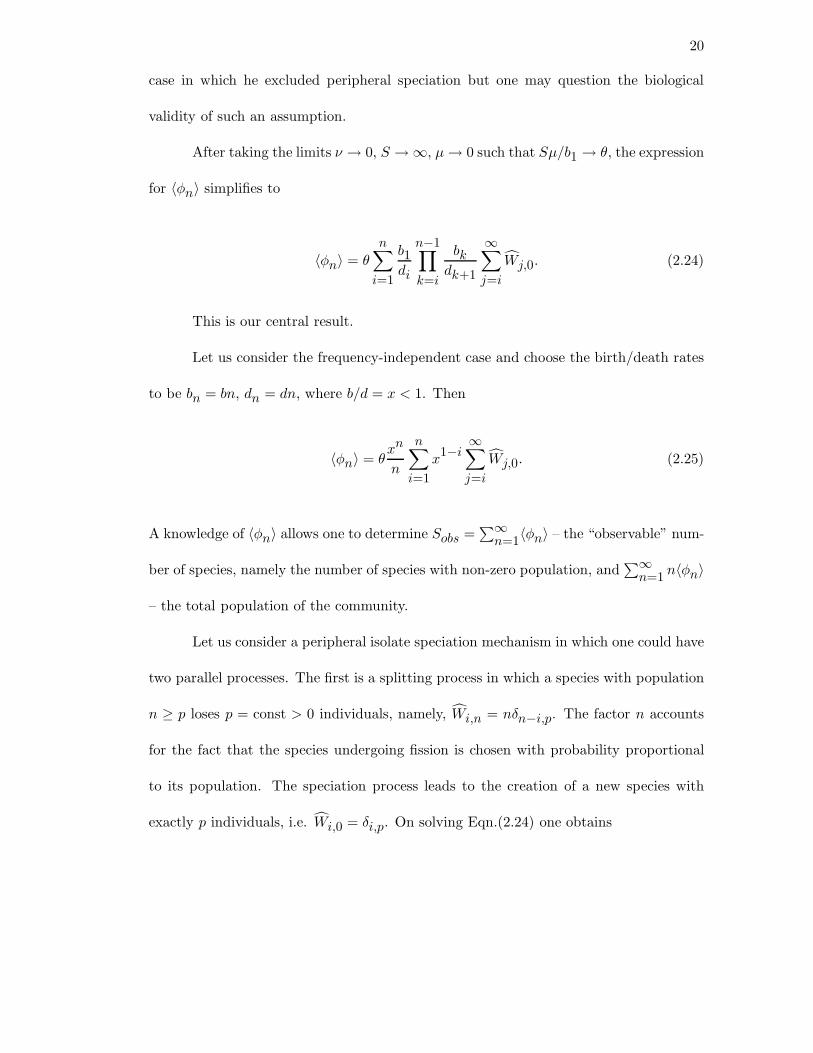
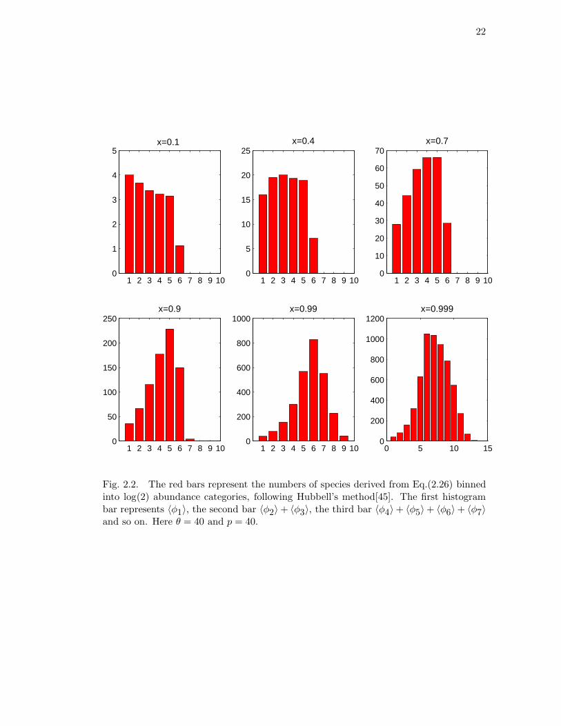
exactly p individuals, i.e. Wi,0 = δi,p. On solving Eqn.(2.24) one obtains
21
〈φn〉 = θx
1 − x
[1 − xn
nΘ(p − n − 1) +
1 − xp
xpxn
nΘ(n − p)
], (2.26)
where Θ(k) = 1 if k > 0 and zero otherwise (see Figure 2.2).
When p = 1 the above formula reduces to the well-known Fisher log-series: 〈φn〉 =
θxn/n, n > 0.
Note that one can obtain an exact analytical solution of Eqn.(2.22) in equilibrium
for arbitrary ν. Strikingly, one obtains the same form of the solution for 〈φn〉 as in
Eqn.(2.26) except that x is replaced by y with x = y[1+ν(1−yp)/(1−y)]. As expected,
x = y, when ν = 0.
22
1 2 3 4 5 6 7 8 9 100
1
2
3
4
5x=0.1
1 2 3 4 5 6 7 8 9 100
5
10
15
20
25x=0.4
1 2 3 4 5 6 7 8 9 100
10
20
30
40
50
60
70x=0.7
1 2 3 4 5 6 7 8 9 100
50
100
150
200
250x=0.9
1 2 3 4 5 6 7 8 9 100
200
400
600
800
1000x=0.99
0 5 10 150
200
400
600
800
1000
1200x=0.999
Fig. 2.2. The red bars represent the numbers of species derived from Eq.(2.26) binnedinto log(2) abundance categories, following Hubbell’s method[45]. The first histogrambar represents 〈φ1〉, the second bar 〈φ2〉 + 〈φ3〉, the third bar 〈φ4〉+ 〈φ5〉+ 〈φ6〉+ 〈φ7〉and so on. Here θ = 40 and p = 40.
23
2.3 Neutrality and stability of
forest biodiversity – comment on paleodata analysis
The unified neutral theory of biodiversity[45] provides a dynamic null hypothesis
for the assembly of natural communities and has proved to be useful for understanding
the influence of speciation, extinction, dispersal, and ecological drift on some spatial and
temporal scales. Recently, Clark and McLachlan[18] have argued that neutral drift is
inconsistent with paleodata. We show that their analysis is based on a misunderstanding
of neutral theory and that their data alone cannot unambiguously test its validity.
Hubbell’s approach[45] builds on the theory of island biogeography[63], which
asserts that an island or a local community approaches a steady-state species richness
at equilibrium between immigration of species from the much larger metacommunity
source area and local extinction of species on the island or in the local community.
Quite generally, the dynamics of the population of a given species is governed by birth
and death events. The Fisher log-series distribution is obtained in the metacommunity
when the per-capita birth and death rates are independent of the species and speciation
is introduced by ascribing a non-zero probability of the appearance of an individual of a
new species[83]. The characteristic time scale for random evolutionary drift accompanied
by speciation and natural selection is, of course, much longer than the 200 generation
period studied in Ref.[18] and during this time interval, the metacommunity distribution
of relative species abundance ought to be essentially constant.
We now turn to an analysis of the consequences of the assumption that the fossil
pollen record analyzed in Ref.[18] is from 8 local sites. The neutral theory[45, 83] for

24
a local community considers the dynamics of birth and death events accompanied by
a steady flow of individuals from the surrounding metacommunity. When the local
community is semi-isolated from the metacommunity, one may introduce an immigration
rate, which is the probability of immigration from the metacommunity to the local
community. For constant immigration rate (taken to be independent of the species),
immigrants belonging to the more abundant species in the metacommunity will arrive
in the local community more frequently than those of rarer species. For the time scale
of 200 generations, the metacommunity provides a fixed backdrop for the action within
the local community and the key point is that not all species are equivalent during
this limited time scale in the metacommunity – there are some that are more abundant
than others. Indeed, in the local community, unlike in the metacommunity, the original
relative species abundance is recovered after a perturbing influence.
Figure 1 of the Clark and McLachlan paper[18] (reproduced here as Figure 2.3)
is misleading. It is based on simulations of neutral dynamics within a lottery model
and claims to show the divergence among sites with time. One can prove rigorously for
their model, which does not admit extinction, that the variance does not increase indef-
initely with time but levels off on reaching equilibrium. Thus their data merely shows
an approach to equilibrium starting from a zero variance initial condition. Their state-
ment that “drift results in rapid accumulation of among-site variance which is readily
identifiable and would continue to increase until much of the diversity was lost through
extinction” is confused. Apart from the fact that the variance does not grow indefinitely,
the time scale for equilibration in their simulations is vastly different from the evolution-
ary time scales associated with speciation in the metacommunity. Indeed, biodiversity
25
Fig. 2.3. Simulations of neutral dynamics showing the divergence among sites. a,Lottery model, where ten species with identical parameters and responses to stochas-ticity compete for space. b, Results for a single species shown for eight different sites.Abundances diverge with the random accumulation of changes at each site. c, Varianceamong sites increases over time owing to accumulation of the random changes in abun-dance shown in b, as does (d) the coefficient of variation, CV. In c and d, the middle lineindicates the median, and the dashed lines bound 90% of simulated values. This figureand the caption are taken from Ref. [18]
26
is maintained in equilibrium in neutral theory due to the balance between extinction of
species and speciation.
More importantly, the simplified lottery model used as a benchmark does not
capture the basic premise of the unified neutral theory of biodiversity[45], that not all
species are equivalent in the local community because of their unequal abundances in the
metacommunity. Thus the “strong evidence for stabilizing forces in the paleo-record”[18]
is not inconsistent with neutral drift.
27
Chapter 3
Density dependence as an explanation of
tree species abundance and diversity
in tropical forests
3.1 General theory
Density and frequency dependence are familiar mechanisms in population biology,
but it is surprising how rarely their consequences for species diversity and relative species
abundance in communities have been discussed [see Chapter 3 of Ref. [45]]. Here we show
that these mechanisms are sufficient to explain quite precisely the species abundance
patterns in six tropical forest communities on three continents.
The neutral theory of biodiversity provides a convenient theoretical framework
for linking community diversity patterns to the fundamental mechanisms of population
biology (e.g., birth, death and migration) and speciation[45]. The celebrated statisti-
cal distribution for relative species abundance, Fisher’s logseries[35], can be shown to
arise directly from the stochastic equations of population growth under neutrality at the
speciation-extinction equilibrium. More significantly, Fisher’s logseries arises when the
birth and death rates are density independent[83]. According to the theory, the mean
number of species with n individuals, 〈φn〉, in a community at the stochastic speciation-
extinction equilibrium takes the general form: 〈φn〉 = SP0
⟨∏n−1i=0
bi,kdi+1,k
⟩
k, where
〈. . .〉k represents the arithmetic average over all species, S is the average number of
species present in the ecosystem, P0 is a constant, and bi,k and di,k are birth and death

28
rates for the k-th species with i individuals. Here we have subscripted the birth and
the death rates for arbitrary species k to indicate that these rates could, in principle, be
species-specific for an asymmetric community. In contrast, “... symmetry occurs at the
species level when no change in community dynamics or the fates of individuals occurs
upon switching the species of any two given populations in the community. Any given
population behaves as it would previously, despite is new species label, and its effects
on other populations remain the same, regardless of their species labels.” (P. Chesson,
personal communication).
We note that what is important in determining the mean number of species,
〈φn〉, are not the absolute rates of birth or death but their ratio, ri,k =bi,k
di+1,k. Indeed,
〈φn〉 is proportional to 〈r1,kr2,k . . . rn−1,k〉k. This formulation is sufficiently general to
represent communities of either symmetric or asymmetric species. Such a situation could
arise, for example, from niche differences or from differing immigration fluxes resulting
from the different relative abundances of the species in the metacommunity. Hereafter,
however, we consider only the symmetric case of a community of non-interacting species
with identical vital demographic rates. For large community size, this formulation is
equivalent to the case of zero-sum dynamics studied by Hubbell[45].
Let us define rn =bn
dn+1
n+1n , where the factor n+1
n is chosen to obtain rn = x for
the Fisher log-series 〈φn〉 ∝ xn/n. In Fisher’s case, rn does not change with population
density and is an intraspecific parameter that measures the relative vital rates of birth
and death of a population. In order to obtain intraspecific density dependence, rn
becomes a function of the population density n. Within our framework,〈φn+1〉〈φn〉
=
nn+1 rn.
29
We now introduce the modified symmetric theory that captures density depen-
dence (rare species advantage or common species disadvantage). In the modified the-
ory, rn will be a decreasing function of abundance, thereby incorporating density de-
pendence. The equations of density dependence in the per capita birth and death
rates for an arbitrary species of abundance n are:b(n)n = b ·
[1 +
b1n + o
(1n2
)]and
d(n)n = d ·
[1 +
d1n + o
(1n2
)], for n > 0 as the leading terms of a power series in (1/n),
b(n)n = b ·
∑∞l=0
bln−l and
d(n)n = d ·
∑∞l=0
dln−l, where bl and dl are constants. This
expansion captures the essence of density-dependence by ensuring that the per-capita
birth rate-death rate ratios decrease and approach a constant value for large n. This
happens because the higher order terms are negligible. Note that the quantity that con-
trols the RSA distribution is the ratio bn/dn+1. Thus the birth and death rates, bn
and dn, are defined up to multiplicative factors f(n + 1) and f(n) respectively, where
f is any arbitrary well-behaved function. One expects that the per capita birth rate
or the fecundity goes down as the abundance increases whereas the mortality ought to
increase with abundance. Indeed, the per capita death rate can be arranged to be an
increasing function of n, as observed in nature, by choosing an appropriate function f
and adjusting the birth rate appropriately so that the ratio bn/dn+1 remains the same.
For example, the choice f(n) = n/(n+c) yields a constant per capita death rate dn = dn
and a fecundity which decreases with increasing abundance.
This mathematical formulation of density dependence may seem unusual to ecol-
ogists familiar with the logistic or Lotka-Volterra systems of equations, in which density
dependence is typically described as a polynomial expansion of powers of n truncated
30
at the quadratic level. However, this classical expansion is not valid in our context be-
cause the range of n is from 1 to an arbitrarily large value, not to some fixed carrying
capacity. Therefore an expansion in terms of powers of (1/n) is more appropriate. For
this symmetric model, noting that 〈φn〉 = SP0∏n−1
i=0bn
dn+1, one readily arrives at the
following relative species-abundance relationship:
〈φn〉 = θxn
n + c, (3.1)
where x = b/d and for parsimony, we have made the simple assumption that b1 = d1 = c.
The biodiversity parameter, θ, is the normalization constant which ensures that the
average number of species in the community is S and is given by θ = S 1+ccx F−1(1 +
c, 2+c, x), where F (1+c, 2+c, x) is the standard hypergeometric function. The parameter
c measures the strength of the symmetric density dependence in the community, and it
controls the shape of the RSA distribution. Note that when c → 0 (the case of no density
dependence), one obtains the Fisher log-series. In this case, as shown in Ref. [83], θ
captures the effects of speciation.
We now show how Eq.(3.1) estimates the strength of symmetric density depen-
dence that is consistent with the observed RSA distributions of tree species in six large
tropical forest plots on three continents: Barro Colorado Island (BCI), Panama, Yasuni
National Park, Ecuador, Pasoh Forest Reserve, Peninsular Malaysia, Korup National
Park, Cameroon, Lambir Hills National Park, Sarawak, Malaysia and Sinharaja World
Heritage Site, Sri Lanka. These sites plots are part of a global network of large plots
managed by the Center for Tropical Forest Science of the Smithsonian Tropical Research
31
Institute. These New and Old World tropical forests have had long separate ecological
and evolutionary histories, but despite these different histories, the symmetric theory
with density dependence fits each of the RSA distributions very well. Figure 3.1 shows
the fits of Eq.(3.1) and the dispersal limitation model[83] to the data sets of tree abun-
dance data collected from the six permanent plots of tropical forest. These plots are 50
ha except Lambir (52 ha), Yasuni (25 ha) and Sinharaja (25 ha). The results in Table
3.1 and Figure 3.1 show that the RSA data of tree species in these plots are equally well
described both by the density dependent model and the dispersal limitation model[83].
The rare species advantage is illustrated in Figure 3.2 and is of the same order
of magnitude in the different forests. The key quantity that controls the RSA is the
birth to death ratio rn defined above. The curves in Figure 3.2 were derived from the
parameters in Table 3.1, which in turn were obtained from the empirical RSA data using
the maximum likelihood method. At stochastic steady state, community size (mass
balance) is maintained by the slow rate of decline in common species (at large n in
Figure 3.2) exactly balanced by the growth of rare species, and by the very slow input
of new species by speciation.
Several important ecological insights result from this new theory. First, we have
shown that an assumption of asymmetric density dependence, for example, postulating
different carrying capacities for each species, is not necessary to explain patterns of rel-
ative species abundance, at least in these 6 tropical forests: a much simpler symmetric
hypothesis is sufficient. Second, we have shown that the population sizes that exhibit
rare species advantage consistent with the observed RSA data are all quite small. The

32
transition to a Fisher log-series-like value for x = b/d which is slightly less than replace-
ment occurs at what would be considered low tree species populations densities in these
forests (< 1 tree/ha). Third, the theory shows why density dependence is scale depen-
dent and must give way to density independence at large spatial scales on which we have
proved that Fisher’s log-series must apply[83]. This means that density dependence has
a characteristic length scale in these tropical forests, above which the strength of density
dependence must necessarily diminish.
Finally, we have demonstrated that symmetric density dependence gives an equally
sufficient mechanistic explanation for RSA patterns in addition to and independent of
dispersal limitation[83]. In Table 3.1, we show the fits of the two mechanisms to the RSA
data from the 6 forests, from which it is clear that both mechanisms yield fits that cannot
be distinguished statistically in quality. However the ecological explanation that accom-
panies each of these mechanisms is very different. According to the dispersal mechanism,
the explanation for the lower frequency of rare species compared to species of middling
abundance is that rare species are more extinction-prone, and when they go extinct in a
community, they take longer to re-immigrate than common species do. According to the
density dependence mechanism, on the other hand, the reduced steady-state frequency
of rare species arises because populations of rare species grow differentially faster into
higher abundance categories due to a rare-species advantage. An important conclusion
is that one cannot deduce the mechanisms causing a particular RSA pattern from RSA
data alone. Because these mechanisms are not mutually exclusive, it must be left to
empirical research to uncover the relative contributions of each mechanism to observed
RSA patterns. However, we do note one distinction between the two mechanisms. The

33
dispersal limitation mechanism generally implies that one is considering a local commu-
nity into which immigration is possible. However, the density dependence mechanism
can apply equally well to local communities or to the metacommunity. If one general-
izes “immigration” to include speciation events, however, then the “dispersal limitation”
mechanism can apply to the the metacommunity as well.

34
Plot S J θ1 m θ2 c xBCI, Panama 225 21457 48.1 0.09 47.5 1.80 0.9978Yasuni, Ecuador 821 17546 204.2 0.43 213.2 0.51 0.9883Pasoh, Malaysia 678 26554 192.5 0.09 189.5 1.95 0.9932Korup, Cameroon 308 24591 52.9 0.54 53.0 0.24 0.9979Lambir, Malaysia 1004 33175 288.8 0.11 301.0 2.02 0.9915Sinharaja, Sri Lanka 167 16936 27.3 0.55 28.3 0.38 0.9983
Plot L1 L2 Deviance P -valueBCI, Panama −314.0 −315.0 2.0 0.16Yasuni, Ecuador −301.0 −303.6 5.2 0.02Pasoh, Malaysia −363.7 −365.3 3.2 0.07Korup, Cameroon −322.3 −323.1 1.6 0.21Lambir, Malaysia −390.5 −391.2 1.4 0.24Sinharaja, Sri Lanka −258.9 −258.5 0.8 0.37
Table 3.1. Maximum likelihood estimates of the density-dependant symmetric modeland dispersal limitation model[83] parameters (upper table) and comparison between themodels (lower table) for the six data sets of tropical forests. In the six plots coordinatedby the Center for Tropical Forest Science of the Smithsonian (http://www.ctfs.si.edu),we considered trees with diameter at breast height ≥ 10 cm. S is the number of species,J is the total abundance and θ1 and θ2 are the biodiversity parameters in the dispersallimitation model[83] and equation (3.1) respectively (note that θ2 is a function of c, xand S and both models have the same number of fitting parameters). The comparisonof the models was carried out with the likelihood ratio test[3, 30, 40]. The lower tablepresents deviance (twice the difference in the log-likelihoods L1 and L2) between the two
models and the corresponding P -value of the χ2-distribution with one degree of freedom.The main result is that the dispersal limitation model and the simple symmetric densitydependent model presented here are statistically comparable to each other in their abilityto fit the tropical forest data.
35
0 5 100
10
20
30
BCI
0 5 10 150
20
40
Korup
0 5 100
50
100
150
Lambir
0 5 100
50
100
Pasoh
0 5 100
50
100
150
Yasuni
0 5 100
10
20
Sinharaja
Fig. 3.1. Fits of density-dependant symmetric model (red line) and dispersal limitationmodel[83] (blue circles) to the tree species abundance data from the BCI, Yasuni, Pasoh,Lambir, Korup and Sinharaja plots, for trees ≥ 10 cm in stem diameter at breast height(see Table 3.1). The frequency distributions are plotted using Preston’s binning methodas described in Ref. [83]. The numbers on the x-axis represent Preston’s octave classes.
36
100
101
102
103
0.9
1
1.1
1.2
1.3
1.4
1.5
1.6
n
n
BCIKorupYasuniLambirPasohSinharaja
r
Fig. 3.2. Plot of r(n) derived from Eq.(3.1) versus n for the six data sets of tropicaltrees. For large values of n, rn asymptotes at a value slightly less than 1. The BCI data(cyan circles) at small n is almost invisible since it coincides with the Pasoh dataset (redcircles).
37
3.2 Is our approach a neutral theory?
Let us address the issue of what constitutes neutrality. We draw from Peter
Chesson’s definition (private communication and references below): “Symmetry at the
individual level means that the species that an individual belongs to is irrelevant to
its fate or the fates of its off spring. An individual’s species could be changed without
affecting the individual in any other way, and without affecting the impact that the
given individual has on other individuals, regardless of species. This form of symmetry,
symmetry at the individual level, is the actual definition of neutrality applicable to the
models in the recent monograph on neutral theory by Steve Hubbell.” This definition,
while simple and concise, may lead to ambiguity when applied to particular models. As
an example, let us consider the model proposed in McKane et al[67]. In that model birth
and death rates are given by the following expressions:
gn = C∗(1 − µ)n
N
N − n
N − 1+
µ
S
(1 − n
N
)(3.2)
and
rn = C∗(1 − µ)n
N
N − n
N − 1+
µ
S(S − 1)
n
N, (3.3)
where N is the total population, S is the total number of species and µ is the immigration
rate.
It is clear from the description of the dynamical rules governing the evolution that
the system is neutral. Indeed, at each time step one picks a random individual, removes

38
(kills) it and places a new one which is either an offspring of another randomly chosen
individual or an immigrant (for simplicity, let us assume that every species has an equal
chance of receiving an immigrant at each time step).
One the other hand, it is also clear from the above equations that the per-capita
birth and death rates, gn/n and rn/n, are density dependant. Thus it is also possible
to view this model as a non-neutral one in which the fate of each individual depends on
the population of the species it belongs to and thus changing an individual’s species will
affect it’s probabilities of giving birth or dying.
Thus the question arises: is the system described in McKane et al[67] neutral
or not? One cannot answer this question merely by inspecting the governing equations.
Rather one needs information on the basis for the dynamical rules of the system. Indeed,
per capita density dependance in and of itself does not preclude the system from being
neutral.
(Interestingly, the more complete model of McKane et al[67] is not neutral because
it relies on the community interaction matrix. When the matrix elements are chosen
randomly, one ends up with a model that can be viewed as being neutral, which they
studied using a mean field type of approach.)
Similarly, consider a simplified case in which the birth and death rates are given
by
bn = b(n + c) (3.4)
39
and
dn = d(n + c) (3.5)
with c > 0.
Note that equation for the birth rate does not necessarily preclude a “neutral”
interpretation. For example, consider a system with the following dynamics: at each
time step either a birth or a death event happens and the probabilities for these events
are constant and proportional to b and d, respectively. For a given event one has two
options (with the probability for each option also fixed): either one chooses a random
individual or an individual from a randomly chosen species. The first option corresponds
to the linear term in the rhs of the above equations and the second option corresponds
to the constant term. With these rules the dynamics of the birth events in the system
is neutral (see the discussion of the model proposed in McKane et al (2000) above).
While the dynamical rules for the birth rates (Eq. (3)) are biologically meaning-
ful (the constant term may be assigned to immigration processes), the presence of the
constant term in the death process does not have a simple ecological basis. Also, in the
form given above, the per capita death rate decreases as n increases, which is in conflict
with our expectations. This unrealistic form of the death rate does not invalidate our
model because the RSA distribution that we obtained is controlled not by the individual
birth and death rates but by the ratio bn/dn+1. Thus the birth and death rates, bn
and dn, are defined up to multiplicative factors f(n + 1) and f(n) respectively, where
f is any arbitrary well-behaved function. One expects that the per capita birth rate

40
or the fecundity goes down as the abundance increases whereas the mortality ought to
increase with abundance. Indeed, the per capita death rate can be arranged to be an
increasing function of n, as observed in nature, by choosing an appropriate function f
and adjusting the birth rate appropriately so that the ratio bn/dn+1 remains the same.
For example, in a limiting case, the choice f(n) = n/(n + c) yields a constant per capita
death rate dn = dn and a fecundity which decreases with increasing abundance. Thus
the resulting formulae for the actual birth and death rates may not necessarily have a
simple interpretation and may very well be non-neutral in character.
3.3 Relationship between the zero sum rule and our approach
There is a departure in our model from the original “zero-sum dynamics” proposed
in Hubbell’s book[45]. The total population is not held fixed in our approach; instead,
we allow the total population to fluctuate and fix it’s average value by choosing the ratio
b/d < 1. A value of b/d = 1 would lead to an exploding population. The competition
between the species for the finite available resources yields an effective b/d < 1 thereby
placing a constraint on the average total population. Our approach is analogous to that
used in statistical physics (see Ref. [43], pp.193-199). Indeed, the zero-sum assumption
corresponds to the microcanonical ensemble, whereas our model corresponds to the grand
canonical ensemble. In the former ensemble, the total number of particles is fixed; in the
latter the average total number of particles is fixed by introducing a chemical potential
which is a measure of the resources needed for the introduction of a new particle into
the system. By adjusting the value of the chemical potential, one can fix the average
41
total population. In our model, the parameter x is analogous to the chemical potential
(more details in a different context are presented in Volkov et al[84]).
Consider an ecosystem consisting of S species with populations of n1, n2, . . . , nS
individuals. We assume that there is a zero sum rule in effect which constrains the total
population to be exactly N .
Let P (n) denote the probability that a given species contains n individuals. Then
the multivariate distribution is given by the following expression:
P (n1, n2, ...nS) =1
Q
S∏
k=1
P (nk)δ(N − n1 − n2 − ... − nS), (3.6)
where the δ function imposes the zero sum rule and the normalization factor (also referred
to as a partition function) is given by
Q =∑
n1,n2,...,nS
S∏
k=1
P (nk)δ(N − n1 − n2 − ... − nS)
=∑
n1,n2,...,nS
S∏
k=1
P (nk)
∫
γ
dz
2πez(N−n1−n2−...−nS)
=
∫
γ
dz
2πezN
[ ∞∑
n=0
P (n)e−zn
]S
=
∫
γ
dz
2πeg(z), (3.7)
where g(z) = zN − f(z)S and
e−f(z) =∞∑
n=0
P (n)e−zn. (3.8)
42
and the contour γ is parallel to the imaginary axis with all it’s points having a fixed real
part x (i.e. z ∈ γ ⇔ z = x + iy,−∞ < y < +∞ ). The integral is independent of x
provided x is positive[70].
In order to estimate the above integral we will use the method of steepest descent
(see Ref. [70], pp.434-443). The basic idea is that if g(z) is a function with a steep
maximum, a result valid in the large community size limit, the dominant contribution
to the integral arises from z-values in the vicinity of this maximum. Let us denote the
value of z at which the maximum occurs by µ. We thus expand g(z) around µ + i0 so
that g′(µ + i0) = N − f ′(µ + i0)S = 0 and keep the first two non-zero terms (again an
approximation justified for a large system):
Q =
∫ ∞
−∞dy
2πeg(µ)−g′′(µ)y2/2+... ≈ eg(µ)
√g′′(µ)
=eµN−f(µ)S√
−f ′′(µ)S(3.9)
From Eq.(3.8) one can show that
f ′(µ) =
∑∞n=0
nP (n)e−µn
∑∞n=0
P (n)e−µn ≡ 〈n〉 (3.10)
is the average number 〈n〉 of individuals per species. One can therefore determine µ by
solving the equation 〈n〉 = N/S.
Likewise
f ′′(µ) = 〈n〉2 − 〈n2〉 < 0. (3.11)

43
Finally, Eq.(3.7) can be rewritten as
Q =∑
n1,n2,...,nS
S∏
k=1
P (nk)e−µnk (3.12)
so that the “effective” probability becomes Peff (nk) = P (nk)e−µnk .
Thus the effect of considering all species simultaneously constrained by the zero
sum rule is entirely equivalent in the large community size limit to treating the species
as being effectively independent of each other but with their abundances controlled by
the quantity µ, the chemical potential.
Indeed, the zero-sum assumption and our approach of fixing the average total
population do lead to the same result for large systems. For example, the distribution
proposed in Ref. [81], which correctly describes Hubbell’s zero-sum metacommunity
model, converges to the Fisher log-series in the limit of large metacommunity size JM
and k ≪ JM :
〈φk〉M =θΓ(JM + 1)Γ(JM + θ − k)
Γ(JM + 1 − k)Γ(JM + θ)≈ θ
xk
k, (3.13)
where x = e−θ/JM / 1.
One can carry out a self-consistency check that the approximation k ≪ JM is
not unreasonable. Consider, for example, the BCI island data, given approximately by
φn = 47.50.9978n
n+1.8 . The total population of the community is more than 20, 000 and the
total number of species is 225. The number of species with a population of more than
2000 individuals is found to be 0.11, which is effectively zero after discretization. Thus
44
the most abundant species is expected to have a population less than around 10% of
the total population in accord with the empirical observation that the most abundant
species has 1717 trees.
There is a clear advantage, in some instances, to our approach. The complexity
of the analysis is greatly reduced. Indeed, by not imposing a zero-sum constraint (i.e.
by allowing the population of each species to run from zero to infinity), one can treat
the species completely independently but with a controlling chemical potential. Our
assumption of fixing the average population is more biologically meaningful because
ecosystems do undergo fluctuations in their abundance. It is important to note, however,
that the full analysis with zero sum rule is specially valuable for understanding the
behavior of species poor communities[3] (for example communities whose biodiversity
number θ is less than 1).
In simple terms there are two entirely equivalent ways of studying a large commu-
nity. One could require that the total number of individuals is fixed at all times so that
the growth in population of one species can only occur at the expense of the number of
individuals of another. Alternatively, one could consider the different species completely
independently and control their average abundance by an effective birth/death rates ra-
tio less than one. The striking result is that two approaches yield the same behavior for
large community size.
45
3.4 Utility of relative species abundance data for elucidating biological
mechanisms
Consider the dispersal limitation model studied by Volkov et al. [83] with the
biodiversity parameter θ = 50 and the immigration parameter m = 0.1. The top panel
of Figure 3.3 shows the RSA data for this model obtained through the analytic expres-
sion. The middle panel shows two different binnings of the same data underscoring
the sensitivity of the shape of the curve on the binning scheme employed. The bottom
panel shows a graph of rn vs. n deduced from the RSA data using the exact formula:
rn = n+1n
〈φn+1〉〈φn〉
, where φn represents the number of species with abundance n. As-
sume now that we were given the RSA data in the top panel and asked what we could
learn from it. Clearly the dispersal limitation model from which the data was derived
provides a perfect description of the data and one may be tempted to conclude that the
mechanism underlying the data is in fact dispersal limitation with the selected model
parameters. However, a symmetric density dependence mechanism yielding rn vs. n in
the bottom panel would also yield exactly the same RSA data. Furthermore, rn does not
constrain the individual birth and death rates but only their ratio. This provides even
greater flexibility in the range of models and mechanisms that are able to fit the data
exactly. One would expect that the RSA data from six forests would contain additional
information which one might use to identify the biological mechanisms underlying them.
However, as shown in Figure 3.1 and the fitting parameters in Table 3.1, both dispersal
limitation and symmetric density dependence provide plausible explanations for all six

46
forests. Thus exercises of estimating the quality of data fits are useful for ruling out mod-
els or parameter values which do not provide a good description of the data. The more
important task of elucidating the underlying biological mechanisms will need additional
empirical data such as data on dynamics or multivariate probability distributions.
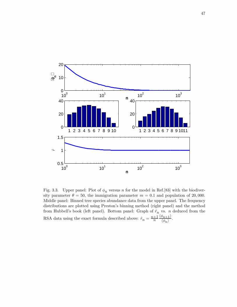
47
100
101
102
103
0
10
20
n
⟨φn⟩
1 2 3 4 5 6 7 8 9 100
20
40
1 2 3 4 5 6 7 8 9 10110
20
40
100
101
102
103
0.5
1
1.5
n
r
Fig. 3.3. Upper panel: Plot of φn versus n for the model in Ref.[83] with the biodiver-sity parameter θ = 50, the immigration parameter m = 0.1 and population of 20, 000.Middle panel: Binned tree species abundance data from the upper panel. The frequencydistributions are plotted using Preston’s binning method (right panel) and the methodfrom Hubbell’s book (left panel). Bottom panel: Graph of rn vs. n deduced from the
RSA data using the exact formula described above: rn = n+1n
〈φn+1〉〈φn〉
.
48
Chapter 4
Spatial scaling relationships in ecology
In this chapter, we take a first step towards the development of an analytically
tractable model that, despite its simplicity, leads to a remarkably accurate quantitative
description of β-diversity in two different tropical forests. It also indicates the existence of
novel scaling behavior, revealing previously unexpected relationships between β-diversity,
RSA, and SAR. The model we study is a version of the well-known voter model [41] which
has been applied to a variety of situations in physics and ecology [26, 78]. The results
presented here were obtained in collaboration with Tommaso Zillio, a doctoral student
in SISSA, Italy.
Let us begin with a phenomenological equation for the time evolution of F (r, t),
the probability density that two randomly drawn individuals separated from each other
by r at time t are of the same species (for simplicity, the system is assumed to be
translationally invariant and F depends only on the separation distance):
F (r, t) =(∇2F (r, t) − γ2F (r, t)
)+ u + sδ(r). (4.1)
where the first term on the right hand side represents dispersal or diffusion; the second is
a decay term arising from the invasion of other species due to speciation or immigration
from a surrounding metacommunity, whose coefficient, γ2, could generally be a function
of r; the u > 0 term allows for the possibility that, in the steady state, F could attain a

49
non-zero value at large distances (as would be expected when the system is dominated
by the effects of immigration [83]); and the last term recognizes that when r is zero, one
has the same species by definition.
The above equation was written down based on general considerations, but it
can also be derived, for example, from the following microscopic model: consider a
hypercubic lattice in d dimensions with each site representing a single individual. At
each time step an individual chosen at random is killed and replaced, with probability
1 − ν with an offspring of one of its nearest neighbors or, with probability ν, with an
individual of a completely new species, not already present in the system throughout
its history. This last process is called speciation and the parameter ν is called the
speciation rate. The special case with ν = 0 has been thoroughly studied (see, for
example, [58, 36, 61, 62, 25]) and on a finite lattice results in a stationary state with just
a single species (monodominance). The more general version with ν 6= 0 has also been
studied [26, 14], but is not as well understood. The equation for F t+1~x
may be written
as
F t+1~x
= F t~x− 2
NF t
~x+
1 − ν
Nd
d∑
µ=1
(F t
~x+µ+ F t
~x−µ
), (4.2)
where ~x denotes the vector separation between two individuals of the same species, N
is the number of sites in the lattice, the sum runs over the basis vector set and one has
the boundary condition F t0
= 1. In steady state, one obtains (with periodic boundary
conditions):
F~x =
∫−π<pi<π
dd~p
(2π)dei~p·~x 1
l(~p)
∫−π<qi<π
dd~q
(2π)d1
l(~q)
, (4.3)

50
d a b z1 0.5 1.05 0.032 0.87 1.2 0.33 0.95 1.21 0.5
Table 4.1. Scaling exponents for d = 1, 2, 3 determined from the scaling collapse of theRSA and SAR plots (Figs. 4.1 and 4.2).
where
l(~p) = −1 +1 − ν
d
d∑
µ=1
cos(pµ). (4.4)
In d = 1
Fr = e−r/ξ , (4.5)
where r ≡ |~x| and the correlation length
ξ =
(ln
1 − ν
1 −√
ν(2 − ν)
)−1
(4.6)
decreases monotonically with increase of ν. In the continuum, one recovers an equation
of the form (4.1) with F (r, t) ≡ F t~x
a−d, γ2 = 2dν/a2, u = 0, and the time has been
rescaled as t → 2dt/a2, where a is the lattice parameter. Note that γ has dimensions
of an inverse length and is proportional to the square root of ν, a fact that we will use
later. The solution of the continuum equation is
F (r) =sγd−2
(2π)d2
(γr)2−d2 K2−d
2
(γr) + u/(γ2), (4.7)
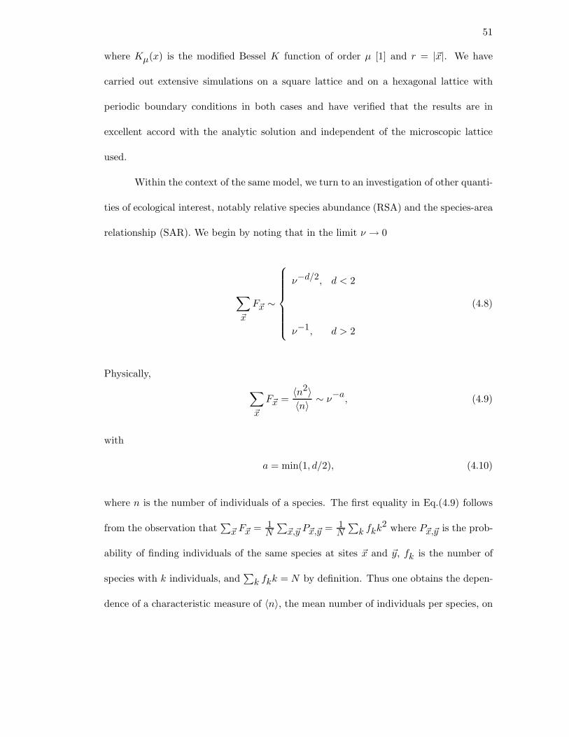
51
where Kµ(x) is the modified Bessel K function of order µ [1] and r = |~x|. We have
carried out extensive simulations on a square lattice and on a hexagonal lattice with
periodic boundary conditions in both cases and have verified that the results are in
excellent accord with the analytic solution and independent of the microscopic lattice
used.
Within the context of the same model, we turn to an investigation of other quanti-
ties of ecological interest, notably relative species abundance (RSA) and the species-area
relationship (SAR). We begin by noting that in the limit ν → 0
∑
~x
F~x ∼
ν−d/2, d < 2
ν−1, d > 2
(4.8)
Physically,
∑
~x
F~x =〈n2〉〈n〉 ∼ ν−a, (4.9)
with
a = min(1, d/2), (4.10)
where n is the number of individuals of a species. The first equality in Eq.(4.9) follows
from the observation that∑
~x F~x = 1N
∑~x,~y P~x,~y = 1
N
∑k fkk2 where P~x,~y is the prob-
ability of finding individuals of the same species at sites ~x and ~y, fk is the number of
species with k individuals, and∑
k fkk = N by definition. Thus one obtains the depen-
dence of a characteristic measure of 〈n〉, the mean number of individuals per species, on
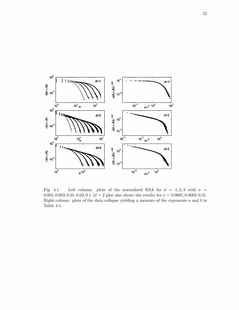
52
Fig. 4.1. Left column: plots of the normalized RSA for d = 1, 2, 3 with ν =0.001, 0.003, 0.01, 0.03, 0.1 (d = 2 plot also shows the results for ν = 0.0001, 0.0003, 0.3).Right column: plots of the data collapse yielding a measure of the exponents a and b inTable 4.1.
53
ν and the identification of a scaling variable nνa. The second scaling variable Aνd/2
follows from dimensional analysis because, as stated before, the speciation length scale is
inversely proportional to the square root of ν. One is therefore led to postulate a scaling
form for the RSA, the number of species f(n, ν,A) with n individuals in an area A (or
volume, if d = 3) when the speciation rate is ν
f(n, ν,A) = n−β f(nνa, Aνd/2). (4.11)
From this equation, one can compute the total number of species S ≡∑n f(n, ν,A)
and a measure of the total area A ≡∑n n f(n, ν,A) (recall that A is equal to the total
number of individuals) as
S ∼ νa(β−1)∫ ∞
νadx x−β f(x,Aνd/2), (4.12)
A ∼ νa(β−2)∫ ∞
νadx x1−β f(x,Aνd/2). (4.13)
The dependence of S in Eq.(4.12) on the area A defines the SAR, i.e. the number
of species S(ν,A) present in an area A when the speciation rate is ν. One can immediately
deduce a scaling form for the SAR:
S(ν,A) = Az S(Aνd/2). (4.14)
54
101
102
103
100
102
A
S
10−1
100
101
102
103
100
102
Aνd/2
S A
−z
102
103
100
102
A
S
10−2
100
102
100
102
Aνd/2
S A
−z
101
102
103
104
100
102
A
S
10−4
10−2
100
102
104
10−1
100
101
102
Aνd/2
S A
−z
d=1
d=2
d=3
d=1
d=2
d=3
Fig. 4.2. Left column: plots of the SAR for d = 1, 2, 3 with ν =0.001, 0.003, 0.01, 0.03, 0.1. Right column: plots of the data collapse yielding a measureof the exponent z in Table 4.1.
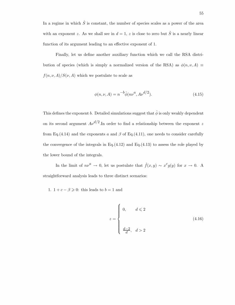
55
In a regime in which S is constant, the number of species scales as a power of the area
with an exponent z. As we shall see in d = 1, z is close to zero but S is a nearly linear
function of its argument leading to an effective exponent of 1.
Finally, let us define another auxiliary function which we call the RSA distri-
bution of species (which is simply a normalized version of the RSA) as φ(n, ν,A) ≡
f(n, ν,A)/S(ν,A) which we postulate to scale as
φ(n, ν,A) = n−bφ(nνa, Aνd/2). (4.15)
This defines the exponent b. Detailed simulations suggest that φ is only weakly dependent
on its second argument Aνd/2.In order to find a relationship between the exponent z
from Eq.(4.14) and the exponents a and β of Eq.(4.11), one needs to consider carefully
the convergence of the integrals in Eq.(4.12) and Eq.(4.13) to assess the role played by
the lower bound of the integrals.
In the limit of nνa → 0, let us postulate that f(x, y) ∼ xcg(y) for x → 0. A
straightforward analysis leads to three distinct scenarios:
1. 1 + c − β > 0: this leads to b = 1 and
z =
0, d 6 2
d−2d , d > 2
(4.16)
56
2. −1 6 1 + c − β < 0: this leads to 1 < b < 2 and the scaling relation
a(2 − b) =d
2(1 − z) (4.17)
3. 1 + c − β < −1: this leads to b = β − c > 2, c = −max(1, d/2) and z = 1.
In order to select between these three cases, we have carried out extensive simula-
tions with hypercubic lattices of various sizes in d = 1, 2, 3. A series of simulations with
fixed size and varying speciation was used for the determination of the RSA fraction of
species (L = 200 for d = 2 and L = 100 for d = 1, 3, L being the side of the hypercube
used). Another series of simulations, varying both the speciation rate and L was carried
out to determine the SAR curves. In this case we consider as the value of S(ν,A) the
mean number of species in a simulation with speciation rate ν on a hypercubic lattice of
size A = Ld.
In order to carry out the collapse, we used the automated procedure described
in [9]. Applying this procedure to the data on the RSA fraction of species obtained by
simulation we were able to obtain the values of the exponents a and b (see Table 4.1,
and Fig.4.1).
Strikingly, in all dimensions b was found to be in the interval (1, 2), confirming
the validity of the second case above. The scaling exponents in Table 4.1 approximately
satisfy Eq.(4.17) . Figure 4.2 shows a collapse plot which confirms the scaling postulates
above. The biggest deviation from our theory can be found in the value of a in d = 2, the
upper critical dimension for diffusive processes. Our results are suggestive of logarithmic

57
corrections but we were not able to find the exact nature of these. Interestingly, our
scaling relation seems to hold even for this case.
58
Chapter 5
Spatial patterns of ecological communities:
α-β diversity and species-area relationship
The spatial model presented in this chapter is based on neutral theory in ecology
[45, 8, 83] and provides a useful starting point for the quantitative study of the role
of interactions and niche differences between species. In tree communities, the spatial
density dependence is known as the Janzen-Connell effect1 [51, 22], which refers to the
negative effect of nearby individuals of a given species on the probability of recruitment,
growth and survival of new individuals of the same species in the community. Note that
the Janzen-Connell effect may be considered as a non-neutral component of otherwise
neutral theory. Indeed, the symmetry on the individual level, which is a key assumption
of neutrality, is broken in the Janzen-Connell mechanism – survival probabilities for
the offsprings depend on the conspecific density and can be regarded as intraspecific
interactions.
1In celebrated papers published more than three decades ago, Janzen [51] and Connell [22]independently hypothesized that tropical forest tree diversity would be enhanced by an inter-action between seed dispersal and density- dependent seed predation. If most seeds fall nearmaternal parents but are killed in the vicinity of the parent by predators and pathogens, and ifthe probability of seed or seedling survival (avoidance of predation) increases with the distancea seed is dispersed from the parent, then tree species will have a reduced probability of replacingthemselves in the next generation in exactly the same location, opening recruitment sites forother tree species in the forest. This spatially structured density dependence will cause a reduc-tion in the probability that two nearby trees are the same species expected from dispersal alone.Over the last two decades, empirical research on large mapped plots of tropical forest have pro-vided increasing evidence for the existence, strength and pervasiveness of Janzen-Connell effectsin species-rich tropical tree communities [87, 38, 46, 2].

59
The community is modeled by a space-filling community of trees of different
species with the following dynamics. A tree, selected at random, is replaced with an
immigrant from the metacommunity (with probability of immigration m) or with an
offspring of one of the neighboring trees (with probability 1 − m) chosen at random.
The metacommunity is assumed to be very large compared with the RSA represented
by the Fisher log-series. The Janzen-Connell effect is captured by introducing a survival
probability for the new tree, which decreases linearly with increase in the number of
conspecific trees in a neighborhood of spatial extent R around the tree. The special case
with R = 0 leads to a simpler model with just the effects of dispersal.
Figure 5.1 shows the results of computer simulations of our model on a hexagonal
lattice with periodic boundary conditions (i.e. a torus to eliminate edge effects) with
the total number of trees equal to JM = 11400. The results we obtain are universal
in that the qualitative behavior is independent of the specific lattice employed or on
the precise shape of the neighborhood around a tree. We depict four cases, Case (1)
the “mean field” approximation, in which choice of the offspring species depends on the
metacommunity relative species abundances and there is no dispersal limitation; Case
(2) in which there are no Janzen-Connell effects (R = 0), but dispersal is limited; Case
(3) in which there are Janzen-Connell effects, but they operate globally (R = ∞); and
case (4) which has intermediate range Janzen-Connell effects (R = 10). In Cases (2) -
(4), we limited dispersal in one time step to between adjacent lattice hexagons. We also
examined the effect of varying the speciation rate.
Case (1), the mean-field approximation with no dispersal limitation and no Janzen-
Connell effects, is fit quite precisely by the Fisher logseries, φn = θxn/n, where θ ∝ JMν

60
(thin blue lines through the black solid and dashed lines). One of the most important
general results is that the Fisher logseries (the mean field case) is supplanted by an RSA
distribution having a mode at intermediate species abundances as soon as one includes
symmetric density dependence in the model. The resulting distribution bears a striking
similarity to ecological data in tropical forests[45]. The distribution of RSA for case (2),
R = 0, and case (3), R = ∞, are very similar – when R is very large, the survival of an
offspring does not depend on the density of its species in its immediate neighborhood and
thus it is similar to the case in which there are no Janzen-Connell effects at all (R = 0).
The most pronounced modal value arises in Case (4), the case with an intermediate
Janzen-Connell length scale, and reflects the fact that the Janzen-Connell density de-
pendence causes community-level frequency dependence (rare species advantage). This
frequency dependence in turn causes species to have more similar relative abundances
at equilibrium.
When the speciation rate, ν, is very small, so that θ ≪ 1 (not shown in Fig. 5.1),
the RSA has a maximum for n = JM and the system approaches monodominance.
The larger the metacommunity, the smaller the value of ν must be in order to obtain
monodominance. Because our metacommunity simulations are for relatively small JM
by comparison with natural communities, the value of ν is chosen to be relatively large.
For rapid speciation, the distribution of RSA is no longer strongly dependent on the
value of R. This is because at high rates of speciation, large numbers of species are
present at steady state in the metacommunity, most of which are at low abundance. In
the numerical case studied, a value of ν = 0.1 results in a mean species abundance of
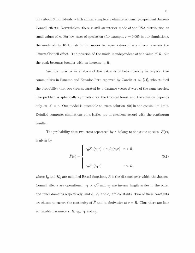
61
only about 3 individuals, which almost completely eliminates density-dependent Janzen-
Connell effects. Nevertheless, there is still an interior mode of the RSA distribution at
small values of n. For low rates of speciation (for example, ν = 0.005 in our simulation),
the mode of the RSA distribution moves to larger values of n and one observes the
Janzen-Connell effect. The position of the mode is independent of the value of R, but
the peak becomes broader with an increase in R.
We now turn to an analysis of the patterns of beta diversity in tropical tree
communities in Panama and Ecuador-Peru reported by Condit et al. [21], who studied
the probability that two trees separated by a distance vector ~x were of the same species.
The problem is spherically symmetric for the tropical forest and the solution depends
only on |~x| = r. Our model is amenable to exact solution [90] in the continuum limit.
Detailed computer simulations on a lattice are in excellent accord with the continuum
results.
The probability that two trees separated by r belong to the same species, F (r),
is given by
F (r) =
c0K0(γ0r) + c1I0(γ0r) r < R;
c2K0(γ1r) r > R,
(5.1)
where I0 and K0 are modified Bessel functions, R is the distance over which the Janzen-
Connell effects are operational, γ1 ∝ √ν and γ0 are inverse length scales in the outer
and inner domains respectively, and c0, c1 and c2 are constants. Two of these constants
are chosen to ensure the continuity of F and its derivative at r = R. Thus there are four
adjustable parameters, R, γ0, γ1 and c0.
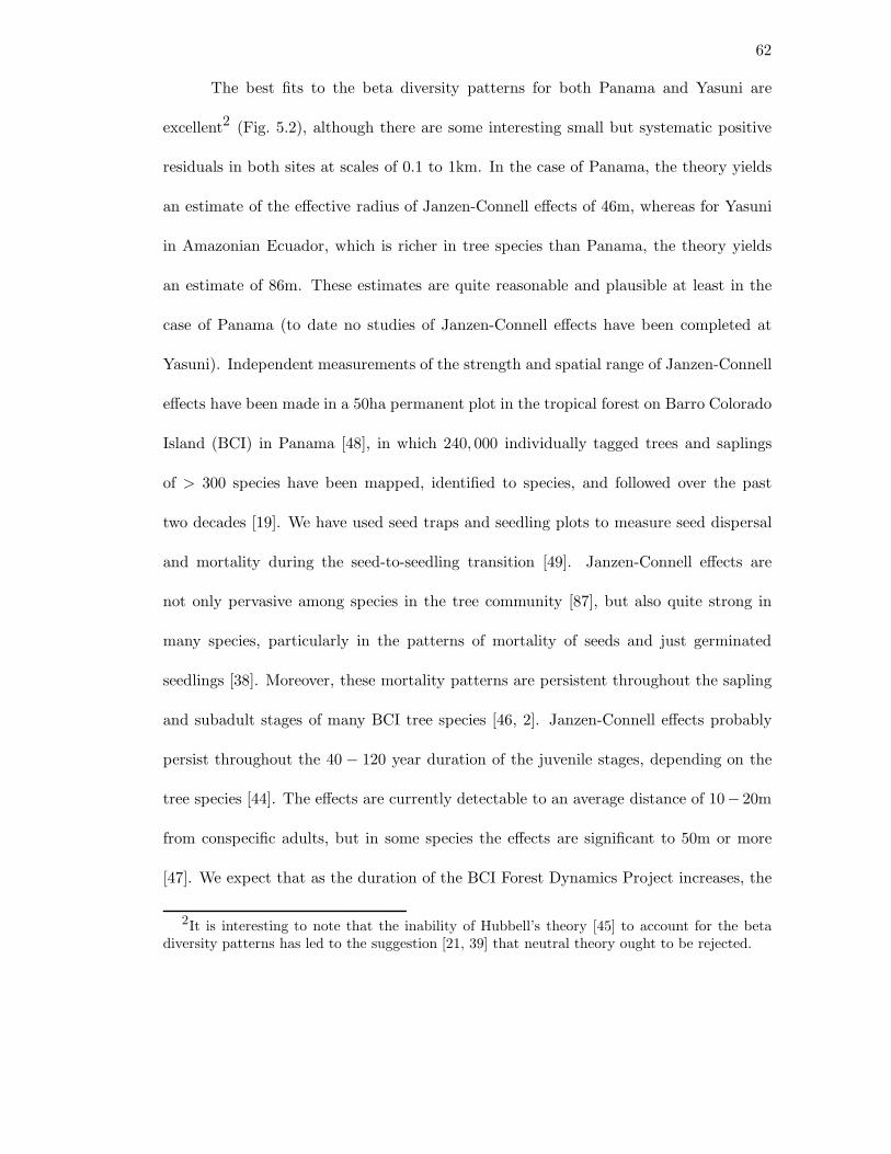
62
The best fits to the beta diversity patterns for both Panama and Yasuni are
excellent2 (Fig. 5.2), although there are some interesting small but systematic positive
residuals in both sites at scales of 0.1 to 1km. In the case of Panama, the theory yields
an estimate of the effective radius of Janzen-Connell effects of 46m, whereas for Yasuni
in Amazonian Ecuador, which is richer in tree species than Panama, the theory yields
an estimate of 86m. These estimates are quite reasonable and plausible at least in the
case of Panama (to date no studies of Janzen-Connell effects have been completed at
Yasuni). Independent measurements of the strength and spatial range of Janzen-Connell
effects have been made in a 50ha permanent plot in the tropical forest on Barro Colorado
Island (BCI) in Panama [48], in which 240, 000 individually tagged trees and saplings
of > 300 species have been mapped, identified to species, and followed over the past
two decades [19]. We have used seed traps and seedling plots to measure seed dispersal
and mortality during the seed-to-seedling transition [49]. Janzen-Connell effects are
not only pervasive among species in the tree community [87], but also quite strong in
many species, particularly in the patterns of mortality of seeds and just germinated
seedlings [38]. Moreover, these mortality patterns are persistent throughout the sapling
and subadult stages of many BCI tree species [46, 2]. Janzen-Connell effects probably
persist throughout the 40 − 120 year duration of the juvenile stages, depending on the
tree species [44]. The effects are currently detectable to an average distance of 10− 20m
from conspecific adults, but in some species the effects are significant to 50m or more
[47]. We expect that as the duration of the BCI Forest Dynamics Project increases, the
2It is interesting to note that the inability of Hubbell’s theory [45] to account for the betadiversity patterns has led to the suggestion [21, 39] that neutral theory ought to be rejected.

63
spatial range over which these significant Janzen-Connell effects are detected will also
increase.
Our simulations of the species-area relationship (SAR) were carried out on two
metacommunities, one with dispersal limitation, and the other with both dispersal lim-
itation and symmetric Janzen-Connell effects. We used a hexagonal lattice with peri-
odic boundary conditions in both cases, we varied the metacommunity size (11, 400 and
46, 000 sites respectively) and we ran the simulations out to 20, 000 death-birth events
on average per site to ensure that equilibrium was reached. We selected 100 sites in the
lattice at random, calculated the SAR, taking each of these sites as the center, and then
we averaged the SAR results over all 100 sites. We calculated SARs for three values of
R (R = 0, R = 10, and R = ∞). We also varied the speciation rate, ν: 0.1, 0.05, 0.01,
0.005 and 0.001.
When plotted in a conventional log-log plot of S versus A, one does obtain three
phases. At short length scales, one has non-universal behavior which depends on the
details of the lattice. At intermediate length scales, one has a power law with an effective
exponent which increases. Finally, in the third phase, there is a linear dependence of S
on A.
Except for very small metacommunity sizes, the species area curves exhibit the
triphasic behavior in a conventional species-area log-log plot (not shown). At short
length scales, one has non-universal behavior which depends on the details of the lattice.
At intermediate length scales, one has a power law with an effective exponent which
increases. Finally, in the third phase, there is a linear dependence of S on A.
64
Strikingly, the data obtained for different areas and speciation rates exhibit a
scaling collapse (see Figure 5.3) consistent with
S ∼ AzFR(νA), (5.2)
where, for large argument the R-dependent scaling function FR(w) ∼ w1−z. The data
confirm the theoretical expectation of a characteristic area per species which is inversely
proportional to the number of species or equivalently the inverse of ν. The effective
values of z for R = 0, 10 and ∞ are 0.28, 0.45 and 0.36 respectively and are in excellent
accord with observational data at intermediate spatial scales. Note that the shallowest
species area curves arise when the Janzen-Connell effects are operational.
Figure 5.4, panels A and B, are snapshots of the species distribution of the two
metacommunities in equilibrium. Each color represents a different species. We chose the
speciation rates so that there is approximately the same number of species (about 110) in
both metacommunities. There are interesting differences between the two landscapes: in
Panel B, with strong Janzen-Connell effects, all of the species patches are approximately
of the same size (approximately equal abundances), whereas in Panel A, the patch sizes
vary considerably (no Janzen-Connell effects). In Panel B, two competing processes affect
the size of the patch: birth/dispersal and Janzen-Connell effects. Because they give rare
species a growth advantage, Janzen-Connell effects reduce the rate of extinction, thereby
increasing the steady-state diversity in the metacommunity. This diversifying effect was
previously reported by Chave et al. [15] and Hubbell and Lake [50].
65
We have shown that the shape of the distribution of relative species abundance in
local communities and the metacommunity is affected by the strength of density depen-
dence, as are steady-state species-area relationships. Questions about the importance
of Janzen-Connell effects in explaining tropical forest tree diversity have been raised
[59] after the discovery of similar Janzen-Connell effects in temperate forests [72]. Our
theory bears on this debate. It shows that Janzen-Connell effects not only influence
the α diversity of tropical forest tree communities on local spatial scales, but also that
they increase species persistence times (times to extinction) and thereby increase the
steady-state species richness at the speciation-extinction equilibrium in the entire meta-
community. However, to our knowledge no data yet exist on the spatial range of such
effects in temperate forests.
In summary, we have demonstrated that the simple model presented here is a
good foundation for the development of a unified understanding of several outstanding
problems in biodiversity. In spite of turning off the interactions and our treatment of
all species in a symmetric manner, our model does an excellent job of capturing the key
features of the observations. This does not mean that an ecosystem is symmetric and
non-interacting. What it does suggest is that the interactions act on top of and in addi-
tion to the demographic processes in the non-interacting system and lead to systematic
but relatively small second-order changes in the statistical properties of the interacting
ecosystem. For example, our non-interacting model produces patchy species distributions
[15] so that the instantaneous pattern of spatial organization of the species in our model
resembles the effects of spatial heterogeneity. In other words, one cannot discern from
the inspection of a “snapshot” whether the heterogeneity has been incorporated into the

66
model or not. Indeed, this patchiness can be thought of as the backdrop provided by
our simplified model, which, in turn, is stabilized by heterogeneous niche effects.
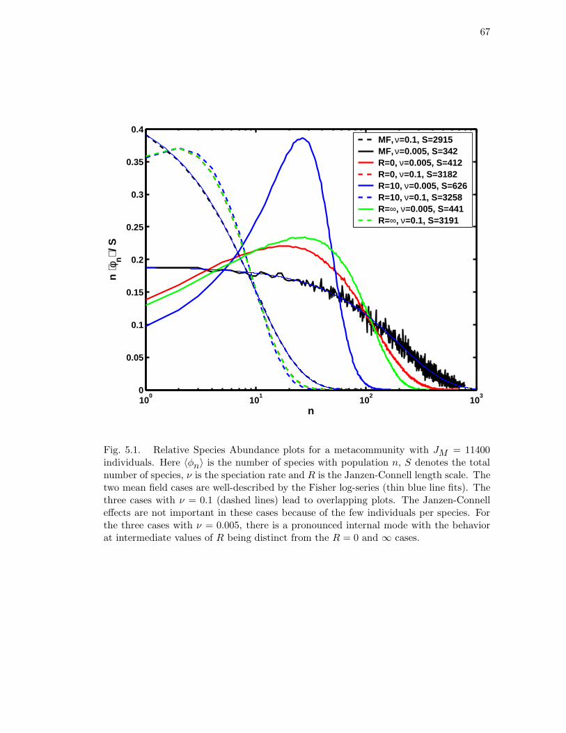
67
100
101
102
103
0
0.05
0.1
0.15
0.2
0.25
0.3
0.35
0.4
n
n ⟨φ
n⟩ /
S
MF, ν=0.1, S=2915MF, ν=0.005, S=342R=0, ν=0.005, S=412R=0, ν=0.1, S=3182R=10, ν=0.005, S=626R=10, ν=0.1, S=3258R=∞, ν=0.005, S=441R=∞, ν=0.1, S=3191
Fig. 5.1. Relative Species Abundance plots for a metacommunity with JM = 11400individuals. Here 〈φn〉 is the number of species with population n, S denotes the totalnumber of species, ν is the speciation rate and R is the Janzen-Connell length scale. Thetwo mean field cases are well-described by the Fisher log-series (thin blue line fits). Thethree cases with ν = 0.1 (dashed lines) lead to overlapping plots. The Janzen-Connelleffects are not important in these cases because of the few individuals per species. Forthe three cases with ν = 0.005, there is a pronounced internal mode with the behaviorat intermediate values of R being distinct from the R = 0 and ∞ cases.
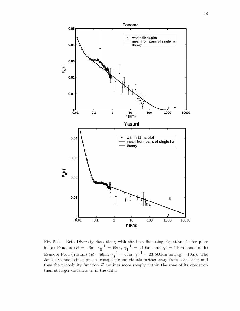
68
0.01 0.1 1 10 100 1000 100000
0.01
0.02
0.03
0.04
0.05Panama
r (km)
F0(r
)
within 50 ha plot mean from pairs of single hatheory
0.01 0.1 1 10 100 1000 100000
0.01
0.02
0.03
0.04
Yasuni
r (km)
F0(r
)
within 25 ha plotmean from pairs of single hatheory
Fig. 5.2. Beta Diversity data along with the best fits using Equation (1) for plots
in (a) Panama (R = 46m, γ−10
= 68m, γ−11
= 210km and c0 = 120m) and in (b)
Ecuador-Peru (Yasuni) (R = 86m, γ−10
= 69m, γ−11
= 23, 500km and c0 = 19m). The
Janzen-Connell effect pushes conspecific individuals further away from each other andthus the probability function F declines more steeply within the zone of its operationthan at larger distances as in the data.
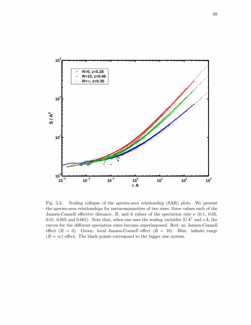
69
10−3
10−2
10−1
100
101
102
103
100
101
102
103
ν A
S /
Az
R=0, z=0.28R=10, z=0.46R=∞, z=0.35
Fig. 5.3. Scaling collapse of the species-area relationship (SAR) plots. We presentthe species-area relationships for metacommunities of two sizes, three values each of theJanzen-Connell effective distance, R, and 6 values of the speciation rate ν (0.1, 0.05,0.01, 0.005 and 0.001). Note that, when one uses the scaling variables S/Az and νA, thecurves for the different speciation rates become superimposed. Red: no Janzen-Connelleffect (R = 0). Green: local Janzen-Connell effect (R = 10). Blue: infinite range(R = ∞) effect. The black points correspond to the bigger size system.

70
Fig. 5.4. Equilibrium snapshots of two metacommunities with no Janzen-Connell effect(R = 0, ν = 0.001, S = 2670, left panel) and Janzen-Connell effect (R = 10, ν = 0.0001,S = 2206, right panel). Even though there is patchiness in both cases, the spatialdistribution of species is quite distinct depending on whether the Janzen-Connell effectsare operational or not.
71
Chapter 6
Organization of ecosystems in
the vicinity of a novel phase transition
An ecological community consists of individuals of different species occupying
a confined territory and sharing its resources[63, 65, 60, 88]. One may draw parallels
between such a community and a physical system consisting of particles. In this chapter,
we show that an ecosystem can be mapped into an unconventional statistical ensemble
and is quite generally tuned in the vicinity of a phase transition where biodiversity and
the use of resources are optimized.
Consider an ecological community, represented by individuals of different species
occupying a confined territory and sharing its common resources, whose sources (for
example, solar energy and freshwater supplies) depend on the area of the territory, its
geography, climate and environmental conditions. The amount of these resources and
their availability to the community may change as a result of human activity and natural
cataclysms such as climate change due to global warming, oil spills, deforestation due to
logging or volcanic eruptions.
Generally, species differ from each other in the amount and type of resources
that they need in order to survive and successfully breed. One may ascribe a positive
characteristic energy intake per individual, εk, of the k-th species (0 < ε0 < ε1 < . . . ),
which ought to depend on the typical size of the individual[77, 12, 68, 73]. The individuals
72
of the k-th species play the role of particles in a physical system housed in the energy
level εk .
We make the simplifying assumption that there is no direct interaction between
the individuals in the ecosystem. Our analysis does not take into account predator-prey
interactions but rather focuses on the competition between species for the same kind of
resources.
In ecology, unlike in physical systems where one has a fixed (average) number
of particles and an associated average energy of the system, one needs to define a new
statistical ensemble. One may define the maximum amount of resources available to the
ecological community to be Emax. The actual energy used by the ecosystem, 〈E〉, can
be no more than Emax
Emax = T + 〈E〉 (6.1)
and, strikingly, as shown later, the energy imbalance, T > 0, plays a dual role. First, for
a given Emax, the smaller the T , the larger the amount of energy utilized by the system.
Thus, in order to make best use of the available resources, a system seeks to minimize this
imbalance. Second, T behaves like a traditional ‘temperature’ in the standard ensembles
in statistical mechanics[34] and, in an ecosystem, controls the relative species abundance.
73
6.1 Sketch of the derivation
Consider the joint probability that the first species has n1 individuals, the second
species has n2 individuals and so on:
Peq(n1, n2, ...) ∝∏
k
P (nk)Θ(Emax −S∑
j=1
εjnj), (6.2)
where S is the total number of species (we assume that S ≫ 1) and Θ(u) is a Heaviside
step-function (defined to be zero for negative argument u and 1 otherwise) which ensures
that the constraint is not violated. Here, P (n) represents the probability that a species
has n individuals in the absence of any constraint and is the same for all species. Note
that P (n) does not have to be normalizable – one can have an infinite population in the
absence of the energy constraint.
As in statistical mechanics[34], the partition function (the inverse of the normal-
ization factor), Q, is obtained by summing over all possible microstates (the abundances
of the species in our case):
Q =∑
{nk}Peq(n1, n2, ...). (6.3)
On substituting Eq. (6.2) into Eq. (6.3) and representing the step-function in the integral
form one obtains
Q =∑
{nk}
∏
k
P (nk)
∫
γ
dz
2πizez(Emax−
∑Sj=1
εjnj) =
∫
γ
dz
2πizezEmax−
∑k h(zεk), (6.4)
74
where e−h(β) =∑
n e−nβP (n) and the contour γ is parallel to the imaginary axis with
all its points having a fixed real part z0 (i.e. z ∈ γ ⇔ z = z0 + iy,−∞ < y < +∞ ).
The integral is independent of z0 provided z0 is positive[70].
We evaluate the integral in Eq. (6.4) by the saddle point method[70] by choosing
z0 in such a way that the maximum of the integrand of Eq. (6.4) occurs when y = 0:
Emax − 1
z0=∑
k
εkh′(z0εk), (6.5)
where the prime indicates a first derivative with respect to the argument. Note that the
rhs is simply∑
k εk〈nk〉 with the average taken with the weight P (nk) exp[−z0εknk].
Comparing Eq. (6.5) with Eq. (6.1), one can make the identification z0 = 1/T
and therefore
Q ∝∑
{nk}
∏
k
P (nk) exp(−εknk/T ). (6.6)
This confirms the role played by the energy imbalance as the temperature of the ecosys-
tem. Indeed, the familiar Boltzmann factor is obtained independent of the form of
P (nk). Note that Eq. (6.6) with P (n) = 1 leads to a system of non interacting identical
and indistinguishable Bosons, whereas P (n) = 1/n! describes distinguishable particles
obeying Boltzmann statistics. It is important to note that terms neglected in the eval-
uation of the integral in Eq. (6.4) contribute for finite size systems but these vanish in
the thermodynamic limit.
In order to derive an expression P (n), consider the dynamical rules of birth, death
and speciation in an ecosystem. In the simplest scenario[45], the birth and death rates
75
per individual may be taken to be independent of the population of the species, with
the ratio of these rates denoted by x. Furthermore, when a species has zero population,
we ascribe a non-zero probability of creating an individual of the species (speciation).
Without loss of generality, we choose this probability to be equal to the per capita birth
rate.
One may write down a master equation for the dynamics[82, 83, 39] and show
that the steady state probability of having n individuals in a given species, P (n), is given
by the distribution:
P (n) = P (0)xn
n, n = 1, 2, 3, ... (6.7)
When x is less than 1, this leads to the classic Fisher log-series distribution[35] for the
average number of species having a population n, φ(n) ∝ P (n).
On substituting Eq. (6.7) into Eq. (6.6), one obtains
Q ∝∑
{nk}
∏
k
[x exp(−εk/T )]nk
nk, (6.8)
where the term [x exp(−εk/T )]nk/nk is replaced by 1 when nk = 0. Note that this
leads to an effective birth to death rate ratio equal to x exp(−εk/T ) < 1 for the k-th
species. In a non-equilibrium situation, such as an island with abundant resources and
no inhabitants, the ratio of births to deaths can be bigger than 1 leading to a build-
up of the population. In steady state, however, the deaths are balanced by births and
speciation (creation of individuals of new species).
76
It is interesting to consider an ecosystem with an additional ceiling on the total
number of individuals, Nmax, that the territory can hold. In analogy with physics, one
may define a chemical potential[34], µ 6 0, so that its absolute value is the basic energy
cost for introducing an individual into the ecosystem. Thus the total energy cost for
introducing an additional individual of the k-th species into the ecosystem is equal to
εk − µ – effectively, all the energy levels are shifted up by a constant amount equal to
this basic cost.
The chemical potential may also be defined as the negative of the ratio of the
energy imbalance to the population imbalance:
µ = −Emax − 〈E〉Nmax − 〈N〉 = − T
Nmax − 〈N〉 , (6.9)
where 〈N〉 is the average population. It follows then that
Nmax = − 1
ln(α)+ 〈N〉, (6.10)
where α = exp(µ/T ) 6 1. This equation has the same structure as Eq. (6.1). Inter-
estingly, the link between the population imbalance and the chemical potential can also
be established formally starting from Eq. (6.2), but with an additional ceiling on the
total number of individuals. The introduction of the ceiling on the population leads to
an additional suppression of the effective birth to death rate ratio which now becomes
αx exp(−εk/T ).
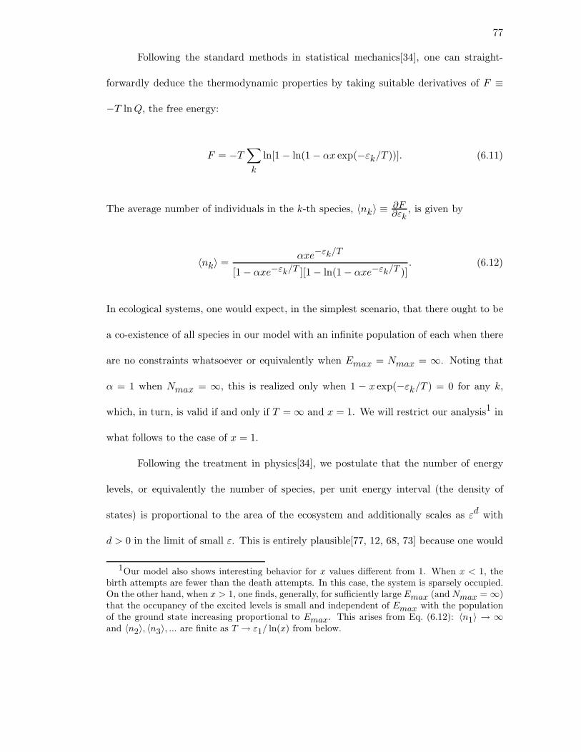
77
Following the standard methods in statistical mechanics[34], one can straight-
forwardly deduce the thermodynamic properties by taking suitable derivatives of F ≡
−T ln Q, the free energy:
F = −T∑
k
ln[1 − ln(1 − αx exp(−εk/T ))]. (6.11)
The average number of individuals in the k-th species, 〈nk〉 ≡ ∂F∂εk
, is given by
〈nk〉 =αxe−εk/T
[1 − αxe−εk/T ][1 − ln(1 − αxe−εk/T )]. (6.12)
In ecological systems, one would expect, in the simplest scenario, that there ought to be
a co-existence of all species in our model with an infinite population of each when there
are no constraints whatsoever or equivalently when Emax = Nmax = ∞. Noting that
α = 1 when Nmax = ∞, this is realized only when 1 − x exp(−εk/T ) = 0 for any k,
which, in turn, is valid if and only if T = ∞ and x = 1. We will restrict our analysis1 in
what follows to the case of x = 1.
Following the treatment in physics[34], we postulate that the number of energy
levels, or equivalently the number of species, per unit energy interval (the density of
states) is proportional to the area of the ecosystem and additionally scales as εd with
d > 0 in the limit of small ε. This is entirely plausible[77, 12, 68, 73] because one would
1Our model also shows interesting behavior for x values different from 1. When x < 1, thebirth attempts are fewer than the death attempts. In this case, the system is sparsely occupied.On the other hand, when x > 1, one finds, generally, for sufficiently large Emax (and Nmax = ∞)that the occupancy of the excited levels is small and independent of Emax with the populationof the ground state increasing proportional to Emax. This arises from Eq. (6.12): 〈n1〉 → ∞and 〈n2〉, 〈n3〉, ... are finite as T → ε1/ ln(x) from below.
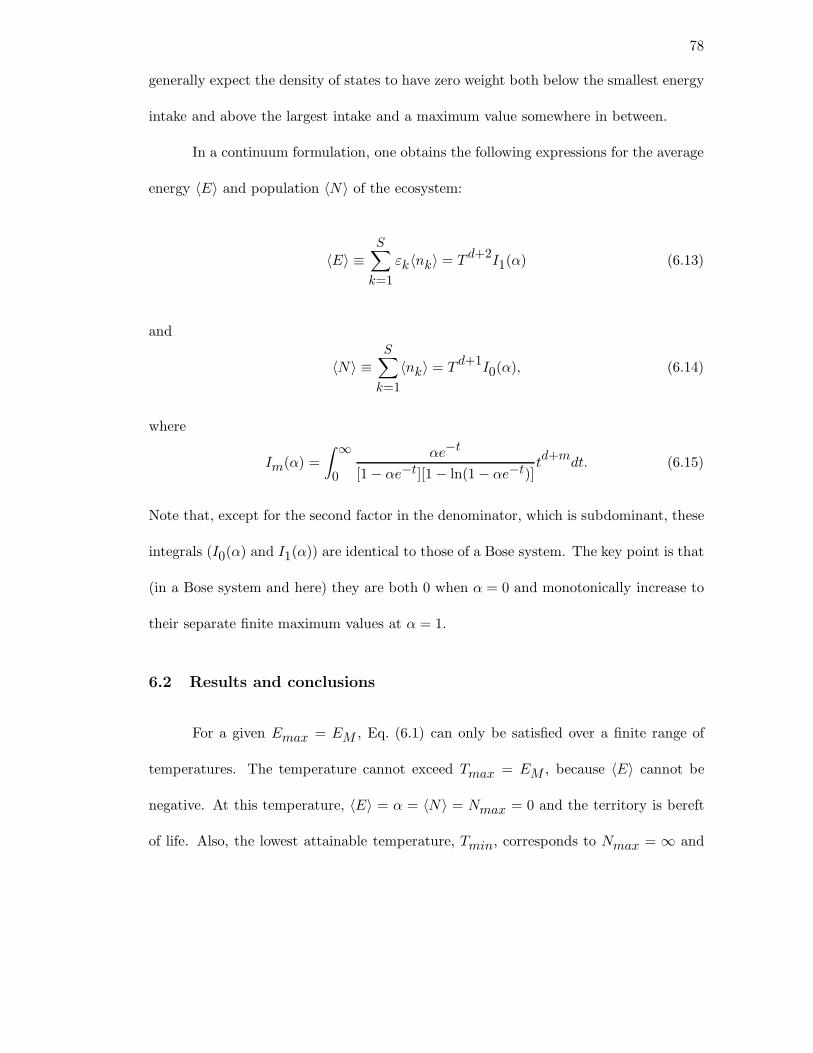
78
generally expect the density of states to have zero weight both below the smallest energy
intake and above the largest intake and a maximum value somewhere in between.
In a continuum formulation, one obtains the following expressions for the average
energy 〈E〉 and population 〈N〉 of the ecosystem:
〈E〉 ≡S∑
k=1
εk〈nk〉 = Td+2I1(α) (6.13)
and
〈N〉 ≡S∑
k=1
〈nk〉 = Td+1I0(α), (6.14)
where
Im(α) =
∫ ∞
0
αe−t
[1 − αe−t][1 − ln(1 − αe−t)]td+m
dt. (6.15)
Note that, except for the second factor in the denominator, which is subdominant, these
integrals (I0(α) and I1(α)) are identical to those of a Bose system. The key point is that
(in a Bose system and here) they are both 0 when α = 0 and monotonically increase to
their separate finite maximum values at α = 1.
6.2 Results and conclusions
For a given Emax = EM , Eq. (6.1) can only be satisfied over a finite range of
temperatures. The temperature cannot exceed Tmax = EM , because 〈E〉 cannot be
negative. At this temperature, 〈E〉 = α = 〈N〉 = Nmax = 0 and the territory is bereft
of life. Also, the lowest attainable temperature, Tmin, corresponds to Nmax = ∞ and
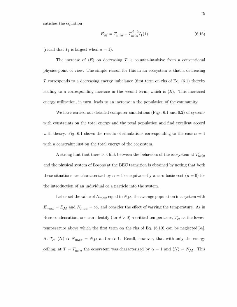
79
satisfies the equation
EM = Tmin + Td+2min
I1(1) (6.16)
(recall that I1 is largest when α = 1).
The increase of 〈E〉 on decreasing T is counter-intuitive from a conventional
physics point of view. The simple reason for this in an ecosystem is that a decreasing
T corresponds to a decreasing energy imbalance (first term on rhs of Eq. (6.1) thereby
leading to a corresponding increase in the second term, which is 〈E〉. This increased
energy utilization, in turn, leads to an increase in the population of the community.
We have carried out detailed computer simulations (Figs. 6.1 and 6.2) of systems
with constraints on the total energy and the total population and find excellent accord
with theory. Fig. 6.1 shows the results of simulations corresponding to the case α = 1
with a constraint just on the total energy of the ecosystem.
A strong hint that there is a link between the behaviors of the ecosystem at Tmin
and the physical system of Bosons at the BEC transition is obtained by noting that both
these situations are characterized by α = 1 or equivalently a zero basic cost (µ = 0) for
the introduction of an individual or a particle into the system.
Let us set the value of Nmax equal to NM , the average population in a system with
Emax = EM and Nmax = ∞, and consider the effect of varying the temperature. As in
Bose condensation, one can identify (for d > 0) a critical temperature, Tc, as the lowest
temperature above which the first term on the rhs of Eq. (6.10) can be neglected[34].
At Tc, 〈N〉 ≈ Nmax = NM and α ≈ 1. Recall, however, that with only the energy
ceiling, at T = Tmin the ecosystem was characterized by α = 1 and 〈N〉 = NM . This
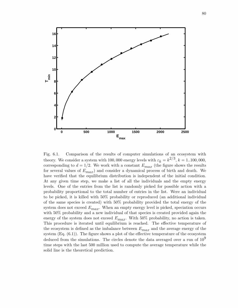
80
0 500 1000 1500 2000 25000
2
4
6
8
10
12
14
16
Emax
Tm
in
Fig. 6.1. Comparison of the results of computer simulations of an ecosystem with
theory. We consider a system with 100, 000 energy levels with εk = k2/3, k = 1..100, 000,corresponding to d = 1/2. We work with a constant Emax (the figure shows the resultsfor several values of Emax) and consider a dynamical process of birth and death. Wehave verified that the equilibrium distribution is independent of the initial condition.At any given time step, we make a list of all the individuals and the empty energylevels. One of the entries from the list is randomly picked for possible action with aprobability proportional to the total number of entries in the list. Were an individualto be picked, it is killed with 50% probability or reproduced (an additional individualof the same species is created) with 50% probability provided the total energy of thesystem does not exceed Emax. When an empty energy level is picked, speciation occurswith 50% probability and a new individual of that species is created provided again theenergy of the system does not exceed Emax. With 50% probability, no action is taken.This procedure is iterated until equilibrium is reached. The effective temperature ofthe ecosystem is defined as the imbalance between Emax and the average energy of thesystem (Eq. (6.1)). The figure shows a plot of the effective temperature of the ecosystem
deduced from the simulations. The circles denote the data averaged over a run of 109
time steps with the last 500 million used to compute the average temperature while thesolid line is the theoretical prediction.
81
confirms that Tc = Tmin. The macroscopic depletion of the community population,
when T < Tmin is entirely akin to the macroscopic occupation of the ground state in
BEC (Fig. 6.2).
When T is larger than Tmin, the energy resources are sufficient to maintain the
maximum allowed population and 〈N〉 = NM . Physically, the state at Tmin corre-
sponds to a maximally efficient use of the energy resources so that any decrease in T
below Tmin inevitably leads to a decrease of the population and the biodiversity in the
community. The existence of this novel transition is quite general and is independent of
specific counting rules such as the ones used in the classic examples of distinguishable
and indistinguishable particles[34].

82
0 0.2 0.4 0.6 0.8 1 1.2 1.4 1.6 1.8 20
0.2
0.4
0.6
0.8
1
1.2
1.4
1.6
1.8
T/Tmin
Fig. 6.2. Phase transition in an ecosystem with Nmax = NM = 65 and d = 1/2.
The dashed and solid curves are plots of theoretical predictions of〈N〉NM
and∂〈E〉∂T
TminEM
respectively versus scaled temperature T/Tmin, where Tmin = 11.6 and EM = 1000.The data points denote the results of simulations. ∂〈E〉/∂T is a quantity analogousto the specific heat of a physical system and has the familiar λ shape associated withthe superfluid transition in liquid helium[34]. It was obtained in the simulations as thederivative of the interpolated values of 〈E〉. The continuous phase transition is signaledby the peak in ∂〈E〉/∂T (and the corresponding drop in 〈N〉) on lowering the temperatureand occurs in the vicinity of the temperature Tmin (the transition temperature movescloser to Tmin as the system size increases).
83
Appendix
A novel ensemble in statistical physics
The conventional grand canonical ensemble in physics describes two systems, one
of which (“the reservoir”) has many more degrees of freedom than the other (“the sys-
tem”). They are placed in contact with each other and allowed to exchange both energy
and particles. The average values of the energy and number of particles are controlled
by the temperature T and the chemical potential µ, respectively. The utility of such an
ensemble lies in the fact that it closely represents the conditions under which experiments
are often performed.
Recently, a theoretical scheme for the modification of the grand canonical ensem-
ble has been proposed[84] in the context of an ecosystem. In that ensemble, the system
consists of an infinite number of energy levels and is coupled with a reservoir. The total
energy and number of particles of both the system and the reservoir are fixed at some
predefined values Emax and Nmax, respectively. Again, the particles and the energy
associated with them are permitted to travel back and forth from the system to the
reservoir. It was found both theoretically and via simulations that, in equilibrium, the
temperature T played a dual role: it controlled the average energy 〈E〉 of the system
(as in the conventional approach) and at the same time it was equal to the imbalance
84
between Emax and 〈E〉. The chemical potential also had a dual role: apart from control-
ling the average number of particles 〈N〉, T/|µ| served as an imbalance between Nmax
and 〈N〉.
The above scheme arises naturally in the studies of the dynamics of ecosystems.
Indeed, as a first approximation, an ecosystem can be modeled as a community of non-
interacting individuals (particles) belonging to different species (energy levels). The
concept of finite Emax and Nmax arises from the limited resources available to an
ecosystem such as space, solar radiation and freshwater supplies.
In the simplest ecologically relevant scenario, the probabilities of the birth and
death events (arrival from / departure into the reservoir) in a given level can be chosen to
be density independent or proportional to the current population of the species. A non-
zero birth rate (speciation) is ascribed to unoccupied levels. This leads to a logarithmic
distribution[83] of the the number of individuals in each level.
Our earlier theoretical and computational studies of the model of the ecosystem
showed that in the absence of the constraints on the total population (Nmax = ∞)
an ecosystem may organize in the vicinity of a phase transition akin to Bose-Einstein
condensation. The transition is signalled by the macroscopic depletion of the population
below a critical temperature.
In this 2Appendix, we generalize our previous work by applying our model to sys-
tems obeying Bose-Einstein, Fermi-Dirac and Boltzmann statistics and carrying out both
theoretical and computational studies. We show that for a system with Bose-Einstein
statistics, the results are similar to the previously studied ecology case. Interestingly,
the systems obeying Fermi-Dirac or Boltzmann statistics also exhibit a first order phase
85
transition and, unlike the ecological or Bose-Einstein cases, this behavior is independent
of the density of states. Also, we expand our previous study of ecological systems and
demonstrate that depending on the value of the birth/death rate ratio there exist three
regimes with distinct behaviors.
The outline of the Appendix is as follows. In Section A.1, starting with the
one-step master equation, we provide a derivation of the partition function of the new
ensemble. For Boltzmann statistics, we demonstrate that the correct counting arises
naturally and the Gibbs paradox is averted. In Section A.2, we consider different types
of statistics and develop the numerical algorithms for simulations. Also, we present
the results of the simulations and compare them to theoretical expectations. Finally,
in Section A.3, we discuss the connections between our ensemble and those in classical
physics and consider a few examples of our model.
A.1 Theoretical framework
Consider S independent boxes in which balls (particles) can be inserted or re-
moved. We label the boxes (energy levels) using the numbers 1, 2, .., S. We postulate
that the dynamics of the balls is governed by simple, physically motivated rules. Our
goal will be to determine the steady state configuration of the system under these rules.
Let N represent the total number of balls in the system.
Let us postulate a constant death rate (or removal rate) per ball equal to d. The
rate of insertion (which may be thought of as a birth rate) of a ball into a given box may
be taken generally to be a function, b(n), of n, the number of balls within the box.
86
Let P (t;n) denote the probability that a given box contains n balls at time t.
The time evolution of P is regulated by the master equation[82]:
dP (t;n)
dt= P (t;n + 1)(n + 1)d +
P (t;n − 1)b(n − 1) − P (t;n)(nd + b(n)). (A.1)
The first (second) term on the right hand side corresponds to the removal (insertion)
of a ball from the box containing n + 1 (n − 1) particles leading to an enhancement of
the probability on the left hand side, whereas the last term corresponds to a depletion
of this probability. The stationary solution can be seen to satisfy detailed balance and
corresponds to an equilibrium situation[82] with
P (n) ∝n−1∏
m=0
b(m)
(m + 1)d. (A.2)
It follows that, when there are S boxes, all satisfying the same birth-death rules,
the unique equilibrium solution is
P (n1, n2, ...nS) =S∏
k=1
P (nk). (A.3)
One can readily work out other special cases of the framework we have presented.
If one chooses b(n) = b0(n + 1), one obtains a pure exponential distribution P (n) =
zn(1− z), where z = b0/d, which, in turn, leads to the Bose-Einstein distribution[43] for
non-degenerate energy levels, i.e. P (n1, n2, ...nS) = zN (1 − z)S . On the other hand, if
b(n) = 0 for any n greater than 0 and equal to b0 otherwise, we find P (n) = zn/(1 + z)
87
for n = 0 or 1 and zero for other values of n and the Fermi-Dirac distribution[43]
P (n1, n2, ...nS) = zN /(1+z)S , provided each of the ni’s is 0 or 1 and P (n1, n2, ...nS) = 0
is zero otherwise.
Note, that the same framework lends itself to the study of the species abun-
dance problem in ecology[45, 83, 84]. Consider the dynamical rules of birth, death
and speciation which govern the population of an individual species. In order to en-
sure that the community will not become extinct, speciation may be introduced by
ascribing a non-zero probability of the appearance of an individual of a new species, i.e
b(0) = b0 6= 0. If one chooses b(n) = b0n for n > 0 (this amounts to the assumption
that the birth rate per individual is constant), one obtains the logarithmic distribution
P (n) = [1 − ln(1 − z)]−1zn/n which, in turn, leads to the well-known Fisher log-series
distribution[35], i.e. 〈φn〉 = θzn/n, where θ = S/[1 − ln(1 − z)] and n > 0. Here, 〈φn〉
represents the average number of species (boxes) with population n.
If b(n) = b0 is taken to be constant, one finds the Poisson distribution P (n) =
e−zzn/n!. This leads to P (n1, n2, ...nS) ∝ zN /∏S
k=1nk!, which is the celebrated Boltz-
mann counting in physics in the grand canonical ensemble and where z plays the role
of a fugacity and N =∑
k nk. It is noteworthy that, unlike in conventional classical
treatments[43] in which one obtains an additional factor of N !, here one gets the correct
Boltzmann counting and one avoids the well-known Gibbs paradox in this scheme. If one
were to ascribe energy values εk to each of the boxes and enforce a fixed average total
energy, one would get the standard Boltzmann result that the probability of occupancy
of an energy level ε is proportional to e−βε, where β is proportional to the inverse of
the temperature.
88
Now let us assign the energy εk to the k-th level (box) so that 0 < ε0 < ε1 < . . . ,
and introduce the constraints Emax and Nmax on the total energy and population of
the system.
The partition function for the system with fixed Emax and Nmax may be written
as
Q =∑
{nk}
∏
k
P (nk)Θ(Emax − ε1n1 − ε2n2 − ...)
Θ(Nmax − n1 − n2 − ...), (A.4)
where Θ(x) is the unit step function, equal to 0 for x < 0 and 1 for x > 0.
Using the integral representation for Θ function[70] one can rewrite the above
equation in the following form:
Q =∑
{nk}
∏
k
P (nk)
∫
γ1
dz12πiz1
ez1(Emax−ε1n1−ε2n2−...)
∫
γ2
dz22πiz2
ez2(Nmax−n1−n2−...) =
∫
γ1
dz12πiz1
ez1Emax
∫
γ2
dz22πiz2
ez2Nmax∏
k
∞∑
n=0
P (n)e−(z2+z1εk)n, (A.5)
where the contours γ1,2 are parallel to the imaginary axis with all their points having
a fixed real part x1,2 (i.e. z1,2 ∈ γ1,2 ⇔ z1,2 = x1,2 + iy1,2, −∞ < y1,2 < +∞). The
integral is independent of x1,2 provided x1,2 is positive[70].
89
Let
e−f(x)
=
∞∑
n=0
P (n)e−xn
. (A.6)
Then
Q =
∫
γ1
∫
γ2
dz1dz2eg(z1,z2), (A.7)
where
g(z1, z2) = − ln(z1) − ln(z2) + z1Emax + z2Nmax −
∑
k
f(z2 + z1εk). (A.8)
In order to evaluate the integral in Eq.(A.7) we will apply the steepest descent method[70].
Let us expand g(z1, z2) about the point (x1 + i0, x2 + i0), where it is maximum:
g(z1, z2) ≈ g(x1, x2) − 1
2!gz21
(x1, x2)y21−
1
2!gz22
(x1, x2)y22− gz1,z2
(x1, x2)y1y2, (A.9)
where gzk11
,zk22
≡ ∂k1+k2g(z1,z2)
∂zk11
∂zk22
. Because g(x1, x2) is a maximum,
gz1(x1, x2) = gz2
(x1, x2) = 0. (A.10)
90
Substituting this expression into Eq.(A.7) and performing the integration one obtains
Q =eg(x1,x2)
√gz21
(x1, x2)gz22
(x1, x2) − g2z1,z2
(x1, x2)=
exp[Emax−µNmax
T −∑k f(
εk−µT
)]
√1 −∑k
ε2k+µ2
T 2f ′′(
εk−µT
) (A.11)
Here we omit the constant factor in the expression for Q and replace x1 and x2 by 1/T
and −µ/T , respectively (T > 0 and µ 6 0). Eq.(A.10) yields
Emax = T +∑
k
εkf ′(
εk − µ
T
)(A.12)
and
Nmax = −T
µ+∑
k
f ′(
εk − µ
T
). (A.13)
The free energy, F , is given by
F ≡ −T ln Q = −Emax + µNmax + F0 + F1, (A.14)
where
F0 = T∑
k
f
(εk − µ
T
)(A.15)

91
and
F1 =1
2T ln
1 −
∑
k
ε2k
+ µ2
T 2f ′′(
εk − µ
T
) . (A.16)
The last term, F1, can be neglected for large enough systems because F1/F0 ∝ ln(V )/V ≪
1, where V is the characteristic size of the system.
Using Eq.(A.14), one can find the entropy S:
S = −∂F
∂T= −
∑
k,n
Pn,k(T ) lnPn,k(T )
Pn, (A.17)
where
Pn,k(T ) =Pne−εkn/T
∑m Pme−εkm/T
. (A.18)
The average population of the k-th level is given by
〈nk〉 =∂F
∂εk= f ′
(εk − µ
T
)(A.19)
and the average population and the total energy of the system are defined as 〈N〉 =
∑k〈nk〉 and 〈E〉 =
∑k εk〈nk〉, respectively. Thus one can rewrite Eqs.(A.12) and
(A.13) as
Emax = T + 〈E〉 (A.20)
92
and
Nmax = − 1
ln(α)+ 〈N〉, (A.21)
where α ≡ exp(µ/T ).
The above equations demonstrate the dual role of the temperature and the chem-
ical potential, which was discussed earlier and represent the central result of our deriva-
tion.
Let us postulate that εk = k1/(d+1) with d > −1, i.e. the number of energy levels
per unit energy interval (the density of states) scales as V εd, where V is the size of the
system. In what follows we will work in units in which V is set equal to 1.
In a continuum formulation, one obtains the following expressions for the average
energy 〈E〉 and population 〈N〉 of the ecosystem:
〈E〉 = Td+2I1(α) (A.22)
and
〈N〉 = Td+1I0(α), (A.23)
where
Im(α) = (d + 1)
∫ ∞
0f′[t − ln(α)]t
d+mdt. (A.24)
93
In the next section we will show, by explicitly calculating the integrals in Eq.(A.24),
that for systems with Bose-Einstein, Fermi-Dirac and Boltzmann statistics, I0,1(α) are
0 when α = 0 and monotonically increase as α approaches 1.
From Eqs.(A.20)-(A.23) one can see that, for a given Emax, the temperature T
cannot become lower than some value Tmin, which occurs when there is no constraint
on the total population, i.e Nmax = ∞. Similarly, the system reaches the maximum
T = Emax when Nmax = 0 and the system is empty.
In order to analyze whether the system can undergo a phase transition, we will
use a scheme similar to the familiar one in Bose-Einstein condensation[34]. Let us fix
the value of Nmax in Eq.(A.21) and vary the temperature (this can be done by varying
Emax). At very high temperatures, the values of α are very small and thus one can
neglect the first term (imbalance) in the rhs of Eq.(A.21). This means that the system
is populated to its full capacity Nmax. As we decrease the temperature, α approaches 1
and the imbalance can no longer be neglected (the system undergoes depletion). If I0(1)
is finite then one can introduce a critical temperature Tc
Tc =
(NmaxI0(1)
) 1d+1
(A.25)
above which 〈N〉 ≈ Nmax and below which the system undergoes a rapid depletion.
Note that in our ensemble the imbalance −1/ ln(α) acts as a zero groundstate level in
the conventional grand canonical ensemble: the macroscopic depletion of the population
of the former is analogous to the macroscopic occupation of the groundstate of the latter.
94
Finally, let us note that α = 1 is related to two cases: first, it enters the expression
for Tc and, second, α = 1 when the system has just the Emax constraint (Nmax = ∞).
This suggests that Tmin = Tc provided that Tc exists (i.e. I0(1) is finite). Indeed, let
us consider the following scenario: when Nmax = ∞ the system organizes at Tmin with
some average population NM and from Eq.(A.23) it follows that Tmin =
(NMI0(1)
) 1d+1
.
But this is also the critical temperature for the system with Nmax = NM . Note that
in the simulations the actual transition temperature T ′c
slightly differs from Tc since for
finite Nmax the value of α cannot reach 1.
A.2 Theoretical and numerical results for systems with different statis-
tics
We now consider four distinct cases and demonstrate that the behavior observed
in simulations is in excellent accord with the theoretical predictions.
A.2.1 Boltzmann Statistics (Figures A.1, A.2 and A.3)
A.2.1.1 Theory
For Boltzmann statistics (bn = b and dn = dn) the average population of the k-th
level and Eqs.(A.20) and (A.21) give
〈nk〉 = αre−εk/T , (A.26)
Emax = T + (d + 1)Γ(d + 2)αrTd+2 (A.27)
95
and
Nmax = − 1
lnα+ Γ(d + 2)αrT
d+1, (A.28)
where r = b/d and Γ(x) =∫∞0
tz−1e−tdt is the gamma function.
One can see that I0(1) is finite for any d. Thus the system with Boltzmann
statistics can undergo a first order phase transition (see Figure A.3).
From Eq.(A.26) it follows that the average population of any level cannot exceed
r, hence r should be large (we used r = 100 in simulations).
A.2.1.2 Simulations
At any given time step, a level is randomly picked and a random number R in the
interval [0, 1) is generated. If R < b/(n + 1) and there is sufficient energy and available
particles in the reservoir a birth event occurs (here n is the occupancy of the level). If
R > 1− d and the level is occupied, a death event occurs. Otherwise no action is taken.
Note that in this scheme the birth and death rates are chosen to be bn = b/(n + 1) and
dn = d (this is equivalent to bn = b and dn = dn since only the ratio bn/dn+1 enters the
expression for the probability). This choice is helpful because both bn and dn are finite
for arbitrary n.
The absolute value of b (recall that d = b/r) is not important provided that it is
less than 0.5.
96
A.2.2 Fermi-Dirac Statistics (Figures A.4, A.5, A.6 and A.7)
A.2.2.1 Theory
For Fermi-Dirac statistics (b0 = b, d1 = d) the average population of the k-th
level and Eqs.(A.20) and (A.21) give
〈nk〉 =αre−εk/T
1 + αre−εk/T, (A.29)
Emax = T − (d + 1)Γ(d + 2)Lid+2(−αr)Td+2 (A.30)
and
Nmax = − 1
ln α− Γ(d + 2)Lid+1(−αr)Td+1, (A.31)
where Lin(z) =∑∞
k=1zk/kn is a polylogarithm function.
As in the case of Boltzmann statistics, the system can undergo a phase transition
for any d.
Note that Eq.(A.29) can be represented as
〈nk〉 =e−(εk−µ∗)/T
1 + e−(εk−µ∗)/T, (A.32)
where µ∗ = µ + T ln r is an ‘effective’ chemical potential and when positive can be
associated with the Fermi energy εF . If a system has a constraint on Emax only, then
µ = 0 and εF = T ln r which means that at small temperatures only the levels with
energies less than εF are filled (this effect is shown in Fig. A.6: if one increases r and
decreases T so that T ln r remains finite, one would observe a sharper effect).
97
A.2.2.2 Simulations
The simulation algorithm is analogous to the case of Boltzmann statistics:
At any given time step, a level is randomly picked and a random number R in the interval
[0, 1) is generated. If the level is empty and R < b and there are sufficient energy and
particles in the reservoir a birth event occurs. If R > 1 − d and the level is occupied a
death event occurs. Otherwise no action is taken.
A.2.3 Bose-Einstein Statistics (Figures A.8 - A.14)
A.2.3.1 Theory
For Bose-Einstein statistics (bn = b(n + 1), dn = dn) the average population of
the k-th level and Eqs.(A.20) and (A.21) give
〈nk〉 =αre−εk/T
1 − αre−εk/T, (A.33)
Emax = T + (d + 1)Γ(d + 2)Lid+2(αr)Td+2 (A.34)
and
Nmax = − 1
lnα+ Γ(d + 2)Lid+1(αr)T
d+1. (A.35)
Let us consider the behavior of the system with different values of r.
When r < 1, the system is underpopulated, i.e. 〈nk〉 is finite for any value of T .
Since Lid+2(r) is finite for any value of d > −1, the system undergoes a phase transition.
98
When r = 1, Lid+1(1) diverges when d 6 0 and is finite otherwise. Thus the
system can undergo a continuous phase transition only for a class of density of states
with d > 0 (see Figure A.14).
Finally, when r > 1, one finds, generally, for sufficiently large Emax (and Nmax =
∞) that the occupancy of the excited levels is small and independent of Emax with
the population of the ground state increasing proportional to Emax. This arises from
Eq. (A.33): 〈n1〉 → ∞ and 〈n2〉, 〈n3〉, ... are finite as T → ε1/ ln(r) from below. The
behavior of the system is qualitatively independent of d.
A.2.3.2 Simulations
The simulation algorithm is the following:
At any given time step, a level is randomly picked and a random number R in the interval
[0, 1) is generated. If R < b and there are sufficient energy and particles in the reservoir a
birth event occurs. If R > 1−d and the level is occupied a death event occurs. Otherwise
no action is taken. Note that the birth and death rates are chosen as bn = b and dn = d
(these rates lead to the same ratio bn/dn+1 as bn = b(n + 1) and dn = dn).
A.2.4 Ecological case (Figures A.15 and A.16)
A.2.4.1 Theory
For the ecosystem obeying logarithmic distribution (bn = b(n + δn,0), dn = dn)
the average population of the k-th level is[84]
〈nk〉 =αre−εk/T
[1 − αre−εk/T ][1 − ln(1 − αre−εk/T )]. (A.36)
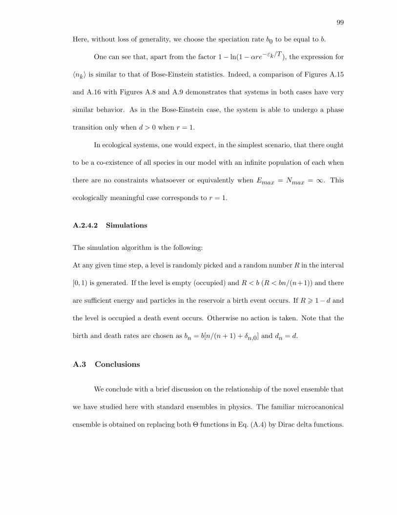
99
Here, without loss of generality, we choose the speciation rate b0 to be equal to b.
One can see that, apart from the factor 1 − ln(1 − αre−εk/T ), the expression for
〈nk〉 is similar to that of Bose-Einstein statistics. Indeed, a comparison of Figures A.15
and A.16 with Figures A.8 and A.9 demonstrates that systems in both cases have very
similar behavior. As in the Bose-Einstein case, the system is able to undergo a phase
transition only when d > 0 when r = 1.
In ecological systems, one would expect, in the simplest scenario, that there ought
to be a co-existence of all species in our model with an infinite population of each when
there are no constraints whatsoever or equivalently when Emax = Nmax = ∞. This
ecologically meaningful case corresponds to r = 1.
A.2.4.2 Simulations
The simulation algorithm is the following:
At any given time step, a level is randomly picked and a random number R in the interval
[0, 1) is generated. If the level is empty (occupied) and R < b (R < bn/(n+1)) and there
are sufficient energy and particles in the reservoir a birth event occurs. If R > 1− d and
the level is occupied a death event occurs. Otherwise no action is taken. Note that the
birth and death rates are chosen as bn = b[n/(n + 1) + δn,0] and dn = d.
A.3 Conclusions
We conclude with a brief discussion on the relationship of the novel ensemble that
we have studied here with standard ensembles in physics. The familiar microcanonical
ensemble is obtained on replacing both Θ functions in Eq. (A.4) by Dirac delta functions.
100
Indeed, by implementing the steepest descent method on Emax term, one obtains the
canonical ensemble whereas on using the steepest descent method on both the Emax
and Nmax terms, one obtains the grand canonical ensemble.
Our numerical scheme is readily modified for the study of the canonical ensemble.
At each timestep, two events occur (provided that the energy constraint is satisfied): two
levels are chosen randomly and a death of a particle in one level is followed by a birth
of the particle in another, provided that the energy constraint is satisfied (otherwise no
action is taken). No action is taken if the first level chosen has no particles in it. We have
implemented this scheme and confirmed that it is in excellent accord with theoretical
expectations.
As a possible application of our model, one can consider the effect of photoex-
citation (and/or photoionization), which occurs when the radiation produced when an
external source interacts with the surrounding atomic gas (e.g., planetary nebulae or OB
star associations embedded in gas clouds[29]). In this case, the processes of birth/death
are represented by excitation/deexcitation (ionization/recombination). The maximum
number of electrons that can possibly go into excited states (or, in the case of ionization,
leave the atom) corresponds to Nmax and the radiation flux can be associated with
Emax. One would expect then that the stimulated emission from the gas will follow the
phase transition scenario described here, i. e. on decreasing Emax below some critical
value one would observe a rapid decline in the flux of stimulated emission.
A more direct example of our ensemble is a shopping game. Consider a con-
sumer shopping in a supermarket. The energy levels correspond to the different types
of products (the products are distinguished from each other by their price only). The
101
total amount of money that the consumer has corresponds to Emax. The analog of
Nmax is the limit on the maximum number of items that the consumer could buy and
is determined, say, by the size of the consumer’s shopping cart. The dynamics of the
game consists of the following rules. The analog of birth is selection of an item from the
store shelf and adding to the cart provided that the number of items in the cart does
not exceed the threshold and provided that the shopper has sufficient money to buy all
the merchandise in the cart. The removal of an item from the cart and returning it to
the shelves corresponds to a death event.
Let us reformulate the rules discussed earlier in the language of this shopping
game. For Boltzmann statistics, the addition event corresponds to the placement of an
item of a randomly picked product in the cart and the death event is the removal of a
random item from the cart. For Bose-Einstein statistics, the addition event is the same
as for Boltzmann statistics and the death event corresponds to the removal of an item of
a randomly picked product already in the cart. For this case, r is a measure of the ratio
of addition to removal attempts. Fermi statistics has the same rules as Bose-Einstein
statistics with the constraint that at most there is just one item in the cart of any given
product. The ecology case consists of addition of an item of a product already contained
in the cart with a probability proportional to the number of such items, a non-zero
probability of the addition of an item of a product not already represented in the cart
and the removal of a randomly picked item present in the cart. Note that the above
rules are not unique and there are many ways to obtain any desired statistics.
Our two key results can be stated as follows. First, the average quantity of money
remaining in the shopper’s wallet (the imbalance) is non-zero and determines the relative
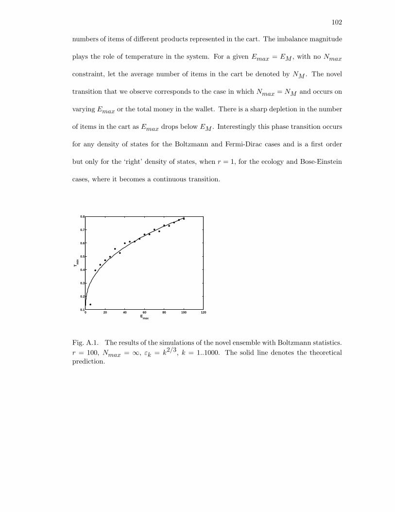
102
numbers of items of different products represented in the cart. The imbalance magnitude
plays the role of temperature in the system. For a given Emax = EM , with no Nmax
constraint, let the average number of items in the cart be denoted by NM . The novel
transition that we observe corresponds to the case in which Nmax = NM and occurs on
varying Emax or the total money in the wallet. There is a sharp depletion in the number
of items in the cart as Emax drops below EM . Interestingly this phase transition occurs
for any density of states for the Boltzmann and Fermi-Dirac cases and is a first order
but only for the ‘right’ density of states, when r = 1, for the ecology and Bose-Einstein
cases, where it becomes a continuous transition.
0 20 40 60 80 100 1200.1
0.2
0.3
0.4
0.5
0.6
0.7
0.8
Emax
Tm
in
Fig. A.1. The results of the simulations of the novel ensemble with Boltzmann statistics.
r = 100, Nmax = ∞, εk = k2/3, k = 1..1000. The solid line denotes the theoreticalprediction.
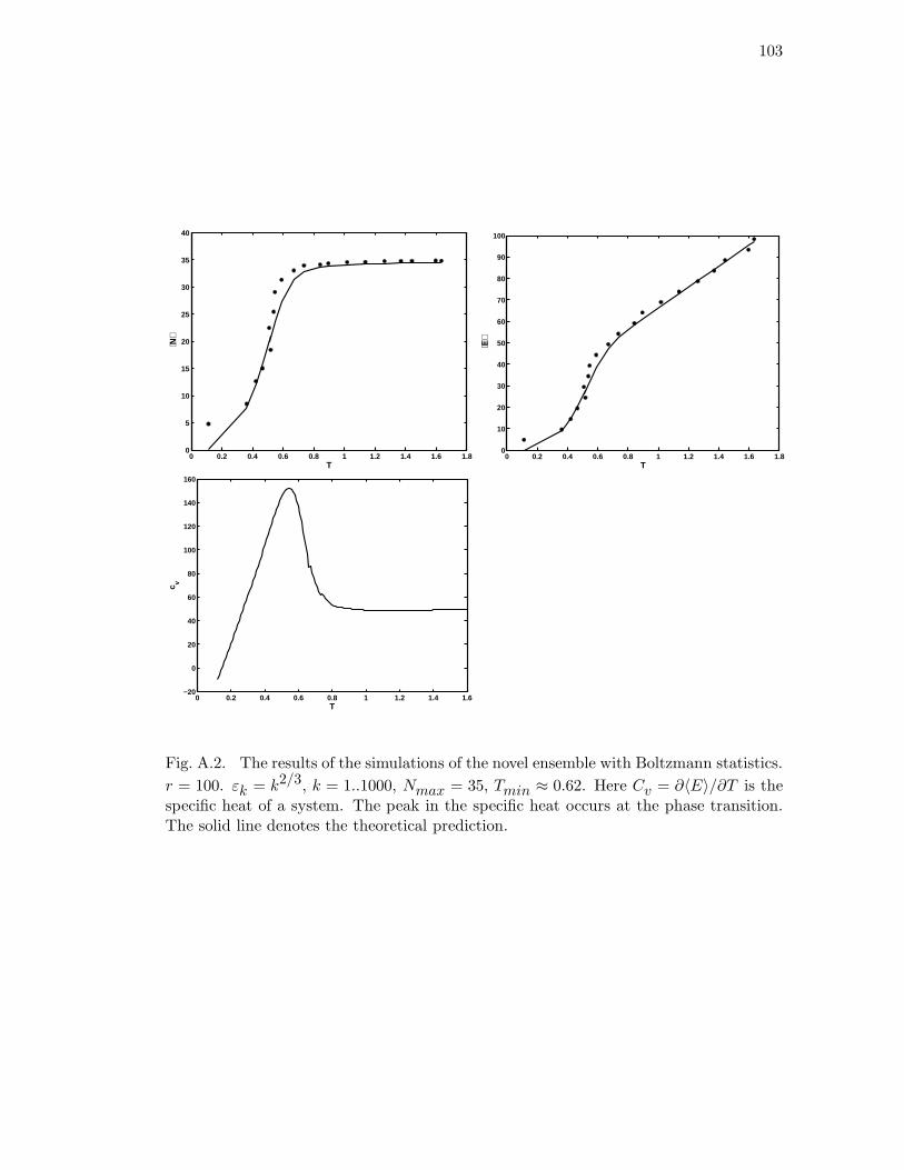
103
0 0.2 0.4 0.6 0.8 1 1.2 1.4 1.6 1.80
5
10
15
20
25
30
35
40
T
⟨N⟩
0 0.2 0.4 0.6 0.8 1 1.2 1.4 1.6 1.80
10
20
30
40
50
60
70
80
90
100
T
⟨E⟩
0 0.2 0.4 0.6 0.8 1 1.2 1.4 1.6−20
0
20
40
60
80
100
120
140
160
T
c v
Fig. A.2. The results of the simulations of the novel ensemble with Boltzmann statistics.
r = 100. εk = k2/3, k = 1..1000, Nmax = 35, Tmin ≈ 0.62. Here Cv = ∂〈E〉/∂T is thespecific heat of a system. The peak in the specific heat occurs at the phase transition.The solid line denotes the theoretical prediction.
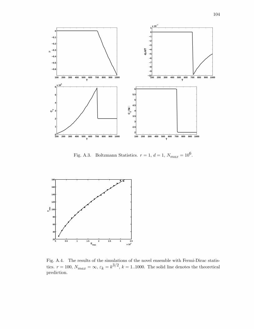
104
100 200 300 400 500 600 700 800 900 1000
−0.6
−0.5
−0.4
−0.3
−0.2
−0.1
0
T
µ
100 200 300 400 500 600 700 800 900 1000−10
−9
−8
−7
−6
−5
−4
−3
−2
−1
0
1x 10
−7
T
dµ/
dT
100 200 300 400 500 600 700 800 900 10000
1
2
3
4
5
6x 10
6
T
Cv
100 200 300 400 500 600 700 800 900 1000
2
2.5
3
3.5
4
4.5
5
5.5
6
T
Cv/⟨N
⟩
Fig. A.3. Boltzmann Statistics. r = 1, d = 1, Nmax = 106.
0 0.5 1 1.5 2 2.5 3 3.5
x 104
20
40
60
80
100
120
140
160
180
Emax
Tm
in
Fig. A.4. The results of the simulations of the novel ensemble with Fermi-Dirac statis-
tics. r = 100, Nmax = ∞, εk = k3/2, k = 1..1000. The solid line denotes the theoreticalprediction.
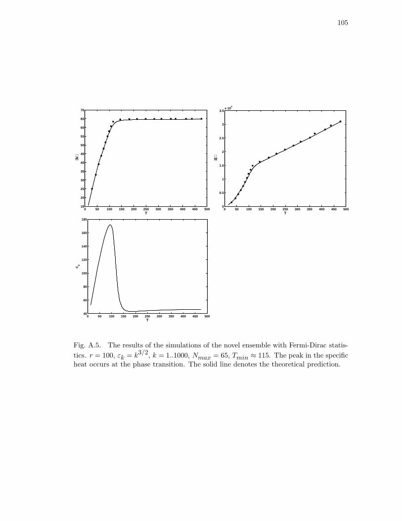
105
0 50 100 150 200 250 300 350 400 450 50015
20
25
30
35
40
45
50
55
60
65
70
T
⟨N⟩
0 50 100 150 200 250 300 350 400 450 5000
0.5
1
1.5
2
2.5
3
3.5x 10
4
T⟨E
⟩
0 50 100 150 200 250 300 350 400 450 50040
60
80
100
120
140
160
180
T
c v
Fig. A.5. The results of the simulations of the novel ensemble with Fermi-Dirac statis-
tics. r = 100, εk = k3/2, k = 1..1000, Nmax = 65, Tmin ≈ 115. The peak in the specificheat occurs at the phase transition. The solid line denotes the theoretical prediction.
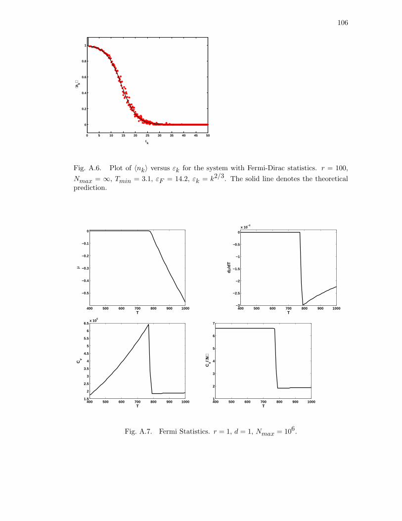
106
0 5 10 15 20 25 30 35 40 45 50
0
0.2
0.4
0.6
0.8
1
εk
⟨nk⟩
Fig. A.6. Plot of 〈nk〉 versus εk for the system with Fermi-Dirac statistics. r = 100,
Nmax = ∞, Tmin = 3.1, εF = 14.2, εk = k2/3. The solid line denotes the theoreticalprediction.
400 500 600 700 800 900 1000
−0.5
−0.4
−0.3
−0.2
−0.1
0
T
µ
400 500 600 700 800 900 1000−3
−2.5
−2
−1.5
−1
−0.5
0x 10
−3
T
dµ/
dT
400 500 600 700 800 900 10001.5
2
2.5
3
3.5
4
4.5
5
5.5
6
6.5x 10
6
T
Cv
400 500 600 700 800 900 10001
2
3
4
5
6
7
T
Cv/⟨N
⟩
Fig. A.7. Fermi Statistics. r = 1, d = 1, Nmax = 106.
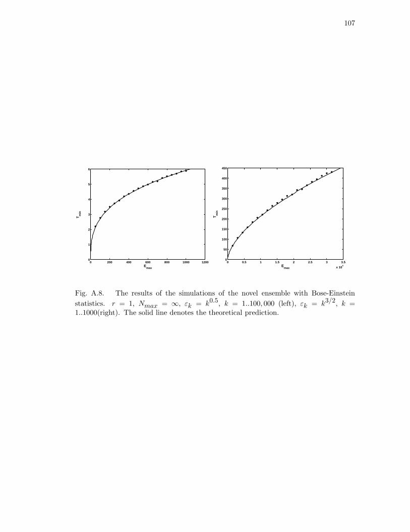
107
0 200 400 600 800 1000 12000
1
2
3
4
5
6
Emax
Tm
in
0 0.5 1 1.5 2 2.5 3 3.5
x 104
0
50
100
150
200
250
300
350
400
450
Emax
Tm
in
Fig. A.8. The results of the simulations of the novel ensemble with Bose-Einstein
statistics. r = 1, Nmax = ∞, εk = k0.5, k = 1..100, 000 (left), εk = k3/2, k =1..1000(right). The solid line denotes the theoretical prediction.
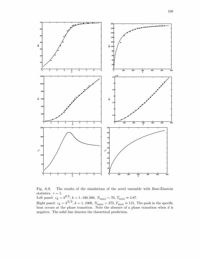
108
1 2 3 4 5 6 7 8 90
10
20
30
40
50
60
70
T
⟨N⟩
0 100 200 300 400 500 6000
20
40
60
80
100
120
140
160
180
200
T
⟨N⟩
1 2 3 4 5 6 7 8 90
200
400
600
800
1000
1200
T
⟨E⟩
0 100 200 300 400 500 6000
0.5
1
1.5
2
2.5
3
3.5x 10
4
T
⟨E⟩
1 2 3 4 5 6 7 8 90
50
100
150
200
250
T
c v
0 100 200 300 400 500 6000
10
20
30
40
50
60
70
80
90
T
c v
Fig. A.9. The results of the simulations of the novel ensemble with Bose-Einsteinstatistics. r = 1.Left panel: εk = k0.5, k = 1..100, 000, Nmax = 70, Tmin ≈ 4.87.
Right panel: εk = k3/2, k = 1..1000, Nmax = 275, Tmin ≈ 115. The peak in the specificheat occurs at the phase transition. Note the absence of a phase transition when d isnegative. The solid line denotes the theoretical prediction.
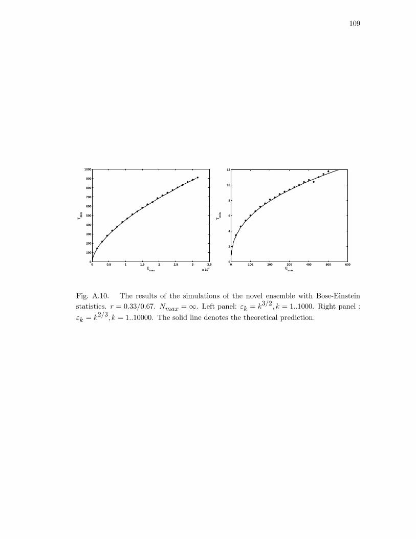
109
0 0.5 1 1.5 2 2.5 3 3.5
x 104
0
100
200
300
400
500
600
700
800
900
1000
Emax
Tm
in
0 100 200 300 400 500 6000
2
4
6
8
10
12
Emax
Tm
in
Fig. A.10. The results of the simulations of the novel ensemble with Bose-Einstein
statistics. r = 0.33/0.67. Nmax = ∞. Left panel: εk = k3/2, k = 1..1000. Right panel :
εk = k2/3, k = 1..10000. The solid line denotes the theoretical prediction.
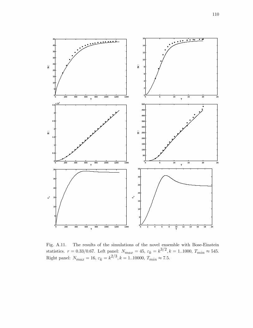
110
0 200 400 600 800 1000 1200 14000
5
10
15
20
25
30
35
40
45
T
⟨N⟩
0 5 10 15 20 250
2
4
6
8
10
12
14
16
T
⟨N⟩
0 200 400 600 800 1000 1200 14000
0.5
1
1.5
2
2.5
3
3.5x 10
4
T
⟨E⟩
0 5 10 15 20 250
50
100
150
200
250
300
350
400
450
500
T
⟨E⟩
0 200 400 600 800 1000 1200 14000
5
10
15
20
25
30
T
c v
0 2 4 6 8 10 12 14 16 18 200
5
10
15
20
25
30
35
T
c v
Fig. A.11. The results of the simulations of the novel ensemble with Bose-Einstein
statistics. r = 0.33/0.67. Left panel: Nmax = 45, εk = k3/2, k = 1..1000, Tmin ≈ 545.
Right panel: Nmax = 16, εk = k2/3, k = 1..10000, Tmin ≈ 7.5.
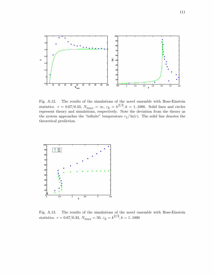
111
0 10 20 30 40 50 60 70 80 90 1000.9
1
1.1
1.2
1.3
1.4
1.5
1.6
Emax
T
0.9 1 1.1 1.2 1.3 1.4 1.5 1.60
10
20
30
40
50
60
70
80
90
100
T
⟨ N⟩
Fig. A.12. The results of the simulations of the novel ensemble with Bose-Einstein
statistics. r = 0.67/0.33, Nmax = ∞, εk = k2/3, k = 1..1000. Solid lines and circlesrepresent theory and simulations, respectively. Note the deviation from the theory asthe system approaches the “infinite” temperature ε1/ ln(r). The solid line denotes thetheoretical prediction.
1 1.5 2 2.5 3 3.50
10
20
30
40
50
60
70
80
90
100
T
<E><N>
Fig. A.13. The results of the simulations of the novel ensemble with Bose-Einstein
statistics. r = 0.67/0.33, Nmax = 50, εk = k2/3, k = 1..1000
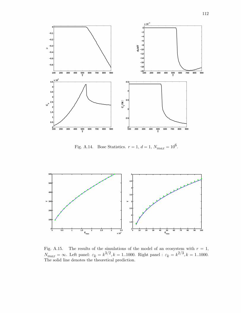
112
100 200 300 400 500 600 700 800 900
−0.6
−0.5
−0.4
−0.3
−0.2
−0.1
0
T
µ
100 200 300 400 500 600 700 800 900−20
−18
−16
−14
−12
−10
−8
−6
−4
−2
0
x 10−4
T
dµ/
dT
100 200 300 400 500 600 700 800 9000
0.5
1
1.5
2
2.5
3
3.5
4
4.5x 10
6
T
Cv
100 200 300 400 500 600 700 800 9002
2.5
3
3.5
4
4.5
T
Cv/⟨N
⟩
Fig. A.14. Bose Statistics. r = 1, d = 1, Nmax = 106.
0 0.5 1 1.5 2 2.5 3 3.5
x 104
0
100
200
300
400
500
600
Emax
T
0 10 20 30 40 50 60 70 80 90 1001
1.5
2
2.5
3
3.5
4
4.5
5
Emax
T
Fig. A.15. The results of the simulations of the model of an ecosystem with r = 1,
Nmax = ∞. Left panel: εk = k3/2, k = 1..1000. Right panel : εk = k2/3, k = 1..1000.The solid line denotes the theoretical prediction.
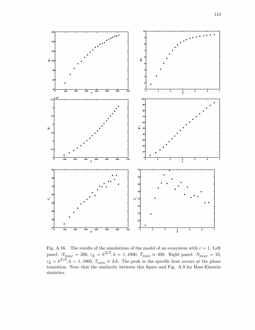
113
0 100 200 300 400 500 600 70040
60
80
100
120
140
160
T
⟨N⟩
1 2 3 4 5 6 71
2
3
4
5
6
7
8
9
10
T
⟨N⟩
0 100 200 300 400 500 600 7000
0.5
1
1.5
2
2.5
3
3.5x 10
4
T
⟨E⟩
1 2 3 4 5 6 70
10
20
30
40
50
60
70
80
90
100
T
⟨E⟩
0 100 200 300 400 500 600 70020
30
40
50
60
70
80
90
T
Cv
1 2 3 4 5 6 78
10
12
14
16
18
20
22
24
T
Cv
Fig. A.16. The results of the simulations of the model of an ecosystem with r = 1. Left
panel: Nmax = 200, εk = k3/2, k = 1..1000, Tmin ≈ 400. Right panel: Nmax = 10,
εk = k2/3, k = 1..1000, Tmin ≈ 3.6. The peak in the specific heat occurs at the phasetransition. Note that the similarity between this figure and Fig. A.9 for Bose-Einsteinstatistics.
114
References
[1] M. Abramowitz and I. A. Stegun. Handbook of Mathematical Functions. Dover,
New York, NY, 1965.
[2] J. Ahumada, S. P. Hubbell, R. Condit, and R. B. Foster. In E. Losos and E. G.
Leigh Jr., editors, Forest Diversity and Dynamism: Findings from a Network of
Large-Scale Tropical Forest Plots. Univ. of Chicago Press, Chicago, Il, in press.
[3] D. Alonso and A. J. McKane. Sampling Hubbell’s neutral theory of biodiversity.
Ecology Letters, 7:911–914, 2004.
[4] M. H. Anderson, J. R. Ensher, M. R. Mathews, C. E. Wieman, and E. A. Cor-
nell. Observation of Bose-Einstein condensation in a dilute atomic vapor. Science,
269:198–201, 1995.
[5] C. K. Augspurger. Seedling survival of tropical tree species: interactions of dispersal
distance, light gaps, and pathogens. Ecology, 65:1705–1712, 1984.
[6] J. Bardeen, L. N. Cooper, and J. R. Schrieffer. Theory of superconductivity. Phys.
Rev., 108:1175–1204, 1957.
[7] G. Bell. The distribution of abundance in neutral communities. Amer. Nat.,
155:606–617, 2000.
[8] G. Bell. Neutral macroecology. Science, 293:2413–2418, 2001.
115
[9] S. M. Bhattacharjee and F. Seno. A measure of data collapse for scaling. J. Phys.
A, 34:6375–6380, 2001.
[10] S. N. Bose. Plancks Gesetz und Lichtquan-tenhypothese. Zeitschr. Physik, 26:178–
181, 1924.
[11] M. T. Boswell, J. K. Ord, and G. P. Patil. Statistical Distributions in Ecological
Work, pages 3–157. International Co-operative Publishing House, Fairland, MD,
1979.
[12] W. A. Calder III. Size, Function, and Life History. Harvard Univ. Press, Cambridge,
Massachusetts, 1984.
[13] T. Caraco. Statistical Distributions in Ecological Work, pages 371–387. International
Co-operative Publishing House, Fairland, MD, 1979.
[14] J. Chave and E. G. Leigh. A spatially explicit neutral model of beta-diversity in
tropical forests. Theor. Popul. Biol., 62:153–168, 2002.
[15] J. Chave, H. C. Muller-Landau, and S. A. Levin. Comparing classical community
models: Theoretical consequences for patterns of diversity. Am. Nat., 159:1–23,
2002.
[16] P. Chesson. A need for niches? Trends in Ecology and Evolution, 6:26–28, 1991.
[17] P. L. Chesson and R. R. Warner. Environmental variability promotes coexistence
in lottery competitive systems. Am. Nat., 117:923–943, 1981.
116
[18] J. S. Clark and J. S. McLachlan. Stability of forest biodiversity. Nature, 423:635–
638, 2003.
[19] R. Condit. Tropical Forest Plots. Springer-Verlag New York, Inc., New York, NY,
1998.
[20] R. Condit, S. P. Hubbell, and R. B. Foster. Density dependence in two understory
tree species in a neotropical forest. Ecology, 75:671–680, 1994.
[21] R. Condit, N. Pitman, E. G. Leigh Jr., J. Chave, J. Terborgh, R. B. Foster, Percy
Nunez V., S. Aguilar, R. Valencia, G. Villa, H. C. Muller-Landau, E. Losos, and
S. P. Hubbell. Beta-diversity in tropical forest trees. Science, 295:666–669, 2002.
[22] J. H. Connell. On the role of natural enemies in preventing competitive exclusion
in some marine animals and in rain forest trees. Dynamics of Populations, pages
298–312, Wageningen, The Netherlands, 1971. PUDOC.
[23] K. B. Davis, M.-O. Mewes, M. R. Andrews, N. J. van Druten, D. S. Durfee, D. M.
Kurn, and W. Ketterle. Bose-Einstein condensation in a gas of sodium atoms. Phys.
Rev. Lett., 75:3969–3973, 1975.
[24] J. Diamond and T. J. Case, editors. Community Ecology. Harper and Row, New
York, NY, 1986.
[25] R. Durrett and S. A. Levin. Stochastic spatial models: a user’s guide to ecological
applications. Phil. Trans. R. Soc. Lond. B, 343:329–350, 1994.
117
[26] R. Durrett and S. A. Levin. Spatial models for species area curves. J. Theoret.
Biol., 179:119–127, 1996.
[27] A. Einstein. Quantentheorie des Einatomi-gen Idealen Gases. Sitz. Ber. Preuss. Ak.
Wiss., 1924:261–267, 1924.
[28] A. Einstein. Quantentheorie des Einatomi-gen Idealen Gases, Zweite Abhandlung.
Sitz. Ber. Preuss. Ak. Wiss., 1925:3–14, 1925.
[29] D. Emerson. Interpreting Astronomical Spectra. John Wiley & Sons, New York,
NY, 1996.
[30] R. S. Etienne. A new sampling formula for neutral biodiversity. Ecology Letters,
8:253–260, 2005.
[31] R. S. Etienne and H. Olff. A novel genealogical approach to neutral biodiversity
theory. Ecology Letters, 7:170–175, 2004.
[32] W. J. Ewens. The sampling theory of selectively neutral alleles. Theor. Popul. Biol.,
3:87–112, 1972.
[33] W. Feller. An Introduction to Probability Theory and Its Applications, Volume 1.
John Wiley & Sons, Hoboken, NJ, 1968.
[34] R. P. Feynman. Statistical Mechanics. Addison-Wesley, Reading, MA, 1998.
[35] R. A. Fisher, A. S. Corbet, and C. B. Williams. The relation between the number of
species and the number of individuals in a random sample of an animal population.
J. of Anim. Ecol., 12:42–58, 1943.
118
[36] L. Frachebourg and P. L. Krapivsky. Exact results for kinetics of catalytic reactions.
Phys. Rev. E, 53:R3009–R3012, 1996.
[37] G. S. Gilbert, S. P. Hubbell, and R. B. Foster. Density and distance-to-adult effects
of a canker disease of trees in a moist tropical forest. Oecologia, 98:100–108, 1994.
[38] K. E. Harms, S. J. Wright, O. Calderon, A. Hernandez, and E. A. Herre. Perva-
sive density-dependent recruitment enhances seedling diversity in a tropical forest.
Nature, 404:493–495, 2000.
[39] J. Harte. Tail of death and resurrection. Nature, 424:1006–1007, 2003.
[40] R. Hilborn and M. Mangel. The Ecological Detective. Confronting Models with Data.
Princeton Univ. Press, Princeton, NJ, 1997.
[41] R. Holley and T. M. Liggett. Ergodic theorems for weakly interacting particle
systems in the voter model. Ann. Probab., 3:643–663, 1975.
[42] B. Houchmandzadeh and M. Vallade. Clustering in neutral ecology. Phys. Rev. E,
68:061912, 2003.
[43] K. Huang. Statistical Mechanics. John Wiley & Sons, New York, NY, 1987.
[44] S. P. Hubbell. In F. Dallmeier and J. A. Comiskey, editors, Forest Biodiversity,
Research, Monitoring and Modeling, volume 20 of Man and the Biosphere Series,
pages 17–44. UNESCO and Parthenon Publishing, Paris, 1999.
[45] S. P. Hubbell. The Unified Neutral Theory of Biodiversity and Biogeography. Prince-
ton Univ. Press, Princeton, NJ, 2001.
119
[46] S. P. Hubbell, J. Ahumada, R. Condit, and R. B. Foster. Local neighborhood effects
on long-term survival of individual trees in a neotropical forest. Ecological Research,
16:859–875, 2001.
[47] S. P. Hubbell, R. Condit, and R. B. Foster. Presence and absence of density de-
pendence in a Neotropical tree community. Trans. Roy. Soc. London. (B), 330:269,
1990.
[48] S. P. Hubbell and R. B. Foster. In Tropical Rain Forest: Ecology and Management,
pages 25–44. Blackwell, Oxford, U.K., 1983.
[49] S. P. Hubbell, R. B. Foster, S. T. O’Brien, K. E. Harms, R. Condit, B. Wechsler,
S. J. Wright, and S. Loo de Lao. Light-Gap Disturbances, Recruitment Limitation,
and Tree Diversity in a Neotropical Forest. Science, 283(5401):554–557, 1999.
[50] S. P. Hubbell and J. Lake. In T. Blackburn and K. Gaston, editors, Macroecology:
Concepts and Consequences, pages 45–63. Blackwell, Oxford, U.K., 2003.
[51] D. H. Janzen. Herbivores and the number of tree species in tropical forest. Am.
Nat., 104:501–528, 1970.
[52] H. Kamerlingh Onnes. Nobel Lectures, volume 1, pages 306–336. Elsevier, Amster-
dam, 1964.
[53] P. L. Kapitsa. Viscosity of liquid helium below the λ-point. Nature, 141:74, 1938.
[54] J. Karlin and J. McGregor. Addendum to a paper of W. Ewens. Theor. Popul.
Biol., 3:113–116, 1972.
120
[55] M. Kimura. Evolutionary rate at the molecular level. Nature, 217:624–626, 1968.
[56] M. Kimura. The Neutral Theory of Molecular Evolution. Cambridge Univ. Press,
Cambridge, UK, 1983.
[57] M. Kimura and T. Ohta. Theoretical Aspects of Population Genetics. Princeton
Univ. Press, Princeton, NJ, 1971.
[58] P. L. Krapivsky. Kinetics of monomer-monomer surface catalytic reactions. Phys.
Rev. A, 45:1067–1072, 1992.
[59] J. H. A. Lambers, J. S. Clark, and B. Beckage. Density dependent mortality and
the latitudinal gradient in species diversity. Nature, 417:732–735, 2002.
[60] S. A. Levin. Fragile Dominion: Complexity and the Commons. Perseus Publishing,
Cambridge, MA, 2000.
[61] T. M. Liggett. Interacting Particle Systems. Springer, New York, NY, 1985.
[62] T. M. Liggett. Stochastic Interacting Systems: Contact, Voter and Exclusion Pro-
cesses. Springer, Berlin, Germany, 1999.
[63] R. H. MacArthur and E. O. Wilson. The Theory of Island Biogeography. Princeton
Univ. Press, Princeton, NJ, 1967.
[64] N. Manokaran, J. V. LaFrankie, K. O. Kochummen, E. S. Quah, J. E. Klahn, P. S.
Ashton, and S. P. Hubbell. Stand Tables and Species Distributions in the Fifty
Hectare Plot at Pasoh Forest Reserve. Forest Research Institute Malaysia, Kuala
Lumpur, Malaysia, 1992.
121
[65] R. M. May. Patterns of species abundance and diversity. In M. L. Cody and J. M.
Diamond, editors, Ecology and Evolution of Communities, pages 81–120. Harvard
Univ. Press, Cambridge, MA, 1975.
[66] B. J. McGill. A test of the unified neutral theory of biodiversity. Nature, 422:881–
885, 2003.
[67] A. McKane, D. Alonso, and R. V. Sole. Mean-field stochastic theory for species-rich
assembled communities. Phys. Rev. E, 62:8466–8484, 2000.
[68] T. A. McMahon and J. T. Bonner. On Size and Life. Scientific American Books,
New York, NY, 1983.
[69] R. J. Morley. Origin and evolution of tropical rainforests. Wiley, New York, NY,
2000.
[70] P. M. Morse and H. Feshbach. Methods of Theoretical Physics, Part I. McGraw-Hill
Book Company, Inc., New York, NY, 1953.
[71] D. D. Osheroff, R. C. Richardson, and D. M. Lee. Evidence for a new phase of solid
He-3. Phys. Rev. Lett., 28:885, 1972.
[72] A. Packer and K. Clay. Soil pathogens and spatial patterns of seedling mortality in
a temperate tree. Nature, 404:478, 2000.
[73] R. H. Peters. The Ecological Implications of Body Size. Cambridge Univ. Press,
Cambridge, UK, 1983.
122
[74] W. H. Press, B. P. Flannery, S. A. Teukolsky, and W. T. Vetterling. Numerical
Recipes in C: The Art of Scientific Computing. Cambridge Univ. Press, Cambridge,
UK, 1993.
[75] F. W. Preston. The commonness and rarity of species. Ecology, 29:254–283, 1948.
[76] C. R. Rao. Statistical Ecology Vol. 1: Spatial Patterns and Statistical Distributions,
pages 131–142. The Penn. State Univ. Press, University Park, PA, 1971.
[77] K. Schmidt-Nielsen. Scaling: Why is Animal Size So Important? Cambridge Univ.
Press, Cambridge, UK, 1984.
[78] J. Silvertown, S. Holtier, J. Johnson, and P. Dale. Cellular automaton models of
interspecific competition for space - the effect of pattern on process. Journal of
Ecology, 80:527–534, 1992.
[79] G. Sugihara, L. Bersier, T. R. E. Southwood, S. L. Pimm, and R. M. May. Predicted
correspondence between species abundances and dendrograms of niche similarities.
Proc. Natl. Acad. Sci., 100:5246–5251, 2003.
[80] D. Tilman. Plant Strategies and the Dynamics and Structure of Plant Communities.
Princeton Univ. Press, Princeton, NJ, 1988.
[81] M. Vallade and B. Houchmandzadeh. Analytical solution of a neutral model of
biodiversity. Phys. Rev. E, 68:061902, 2003.
[82] N. G. Van Kampen. Stochastic Processes in Physics and Chemistry. North-Holland,
Amsterdam, 2001.
123
[83] I. Volkov, J. R. Banavar, S. P. Hubbell, and A. Maritan. Neutral theory and relative
species abundance in ecology. Nature, 424:1035–1037, 2003.
[84] I. Volkov, J. R. Banavar, and A. Maritan. Organization of ecosystems in the vicinity
of a novel phase transition. Phys. Rev. Lett., 92:218703, 2004.
[85] G. A. Watterson. Models for the logarithmic species abundance distributions. Theor.
Popul. Biol., 6:217–250, 1975.
[86] E. Weiher and P. Keddy, editors. Ecological Assembly Rules: Perspectives, Ad-
vances, and Retreats. Cambridge Univ. Press, Cambridge, UK, 1999.
[87] C. Wills, R. Condit, S. P. Hubbell, and R. B. Foster. Strong density- and diversity-
related effects help to maintain tree species diversity in a neotropical forest. Proc.
Natl. Acad. Sci., 94:1252–1257, 1997.
[88] E. O. Wilson. The Future of Life. Knopf, New York, NY, 2002.
[89] S. J. Wright. Plant diversity in tropical forests: a review of mechanisms of species
coexistence. Oecologia, 130:1–14, 2002.
[90] T. Zillio, I. Volkov, J. R. Banavar, S. P. Hubbell, and A. Maritan. unpublished.
Vita
Igor Volkov
Department of Physics
104 Davey Lab
The Pennsylvania State University
University Park, PA 16802-6300
(814) 880-7930 (Phone)
(814) 865-3604 (Fax)
Education
1998 — : Graduate Student at The Pennsylvania State University.
Thesis advisor: Jayanth Banavar
Diploma 1996 : Physics, Belarusian State University, Belarus.
Advisor: Serguei Zavtrak