Nonequilibrium Statistical Physics in Ecology: Vegetation...
174
Nonequilibrium Statistical Physics in Ecology: Vegetation Patterns, Animal Mobility and Temporal Fluctuations PhD THESIS Ricardo Mart´ ınez Garc´ ıa Director: Dr. Crist´ obal L ´ opez 2014
Transcript of Nonequilibrium Statistical Physics in Ecology: Vegetation...

Nonequilibrium Statistical Physics inEcology: Vegetation Patterns, AnimalMobility and Temporal Fluctuations
PhD THESIS
Ricardo Martınez Garcıa
Director:
Dr. Cristobal Lopez2014

Nonequilibrium Statistical Physics in Ecology: Vegetation Patterns, Animal Mobilityand Temporal Fluctuations
Ricardo Martınez GarcıaTesis realizada en el Instituto de Fısica Interdisciplinar y Sistemas Complejos, IFISC (CSIC-UIB).Presentada en el Departamento de Fısica de la Universitat de les Illes Balears.
For an updated version of this thesis please contact:[email protected] or [email protected]
PhD Thesis
Director: Dr. Cristobal Lopez
Palma de Mallorca, 2 de Mayo de 2014.
The cover shows two aerial photographies of vegetation patterns taken from von Hardenberg et al.[2001], and a Mongolian gazelle offspring taken from www.lhnet.org.


Cristobal Lopez Sanchez, Profesor Titular de Universidad
CERTIFICA:
que esta tesis doctoral ha sido realizada por el doctorando Sr. Ricardo MartınezGarcıa bajo su direccion en el Instituto de Fısica Interdisciplinar y SistemasComplejos y, para que conste, firma la presente
Director:
Dr. Cristobal Lopez Sanchez
Doctorando:
Ricardo Martınez Garcıa
Palma de Mallorca,
2 de Mayo de 2014.


A mis padres y hermano.
Look up to the sky.You will never find rainbows
if you are looking down.
Charles Chaplin.

Agradecimientos
En primer lugar, quisiera agradecer a Cristobal el haberme dado la oportunidadde hacer esta tesis doctoral. Gracias por todo lo aprendido, pero sobre todo por tubuen humor y continuo apoyo. Gracias tambien por darme la libertad necesariapara equivocarme y tener mis propias ideas, o al menos intentarlo. I also want tothank Justin Calabrese who I have considered my second PhD supervisor sincemy stay in Front Royal. Thanks for your friendliness and for teaching me so manythings. No quisiera olvidarme de Emilio Hernandez-Garcıa y Federico Vazquez,siempre habeis tenido un rato para sentaros conmigo. Gracias especialmente atı, Fede, por tantas horas juntos delante del ordenador buscando power laws.Finally, thank you Miguel Angel Munoz, Chris Fleming, Thomas Mueller andKirk Olson for spending part of your time on me.
Empezando por el principio, quiero dedicar unas palabras a Juan Francisco, pordedicarme tanto tiempo en el colegio y por despertar el interes por la fısica en mı.Tambien a Daniel Alonso, por ayudarme a recuperarlo, y a Santiago Brouard,por iniciarme en el mundo de la investigacion en La Laguna.
En el IFISC he encontrado el ambiente ideal para disfrutar de esta tesis. Graciasa todos por hacerlo posible. En particular a Marta, Inma, Rosa Campomar yRosa Rodrıguez por hacer de la burocracia algo mas sencillo. A Edu, Ruben,Antonia y David, porque sin su ayuda seguramente esta trabajo no habrıa idopara delante. Espero no haber dado mucho la lata, y si lo he hecho, os debo undesayuno. Siempre estare agradecido a todos mis companeros en la profundidadde la S07. Al Dr. Luis F. Lafuerza, por su acogida durante mi primer verano ypor estar siempre dispuesto a echarme una mano. A Luca: Calvia y Milan nuncaestuvieron tan cerca. A Pablo y Vıctor, por nuestras conversaciones sobre arteprecolombino y vuestro sentido del humor, y a Enrico y Simone, por las clasesgratis de italiano. Muchas gracias tambien a todos los demas: Przemyslaw(espero haberlo escrito bien), Miguel Angel, Pedro, Adrian, Julian, Juan, Xavi,Marie, Ismael, Leo, Alejandro, Toni Perez...
Part of this Thesis has been done in other institutions. I have really enjoyedthese experiences, but they would not have been the same without all the nicepeople that I could meet. Thanks to Nat, Ben, Fan, Meng, Tuya, Leah, Caroline,Bettina, Christian, Jan... for the time in Front Royal, y gracias a Pablo por algunaescapada por Dresden.
ix
x
A nivel institucional, gracias al CSIC y a la Univeristat de les Illes Balears, puessin sus fondos nunca podrıa haber completado este doctorado, y a los proyectosFISICOS e INTENSE@COSYP.
Estos anos en Mallorca han sido mucho mas que anos de trabajo. A traves delfutbol sala he podido conocer a muchısima gente. Gracias a todos, especialmentea mis companeros de La Salle Pont d’Inca por haber sido una familia desde elprimer dia. ¿Que pasa ...? Nombraros a todos ocuparıa mucho espacio, perolo voy a hacer: Bily, Biel, Raul, Xevi, Hector, Colo, Edu, Toni, Roberto, Berni,Baia (gran futuro delante de las camaras), Toni Mir, Pitu, Majoni, Rafa, Alberto,Perillas y Bernat. Muchısimas gracias tambien a todos los ninos que he tenidola inmensa fortuna de entrenar. Sobre todo a los mas pequenos, de quienestenemos muchısimo que aprender.
He tenido la gran suerte de vivir con grandes companeros. Miguel, uno de losmejores amigos que se pueden tener y probablemente la persona con mayorvision de futuro. Mario, importador a Mallorca de la ultima tecnologıa riojana:el motorabo. ¡Dale que suene! Siempre. Juntos hemos compartido muchosde los mejores momentos. Gracias. Gracias Angel por ensenarme la isla y pornuestros momentos de pesca. No me olvido de vosotros, Luis, Gloria, Kike,Laura y Adrian porque por vuestra culpa llegar a Mallorca fue facil e irse seradifıcil.
Estas ultimas lıneas van para la gente que mas quiero. A mis amigos de Tenerife,los de siempre. A Paula, por ser como eres, por tu sonrisa, y por acompanarme.A Guillermo, Barbara y Miki, por preocuparos por mi. Pero sobre todo dedicoeste trabajo a mis padres, por ser el mejor ejemplo y por creer y confiar en mi.Ya que no os lo recuerdo muy a menudo, aprovecho estas palabras para deciroslo mucho que os quiero. A mi hermano, el mejor companero y un ejemplo comocientıfico. Gracias por mis primeros trabajo de campo a los 2 anos. Poca gentetiene la suerte de saber que es un coleoptero antes de ir a la guarderıa1. Porultimo, a mis abuelos, a los que ya no estan Alejandro, Rosa e Isidro y a Cuquita,por poder disfrutarte cada dıa.
1Orden de insectos masticadores que poseen un caparazon duro y dos alas, tambien duras,llamadas elitros, que cubren a su vez dos alas membranosas
Resumen
Esta tesis doctoral se centra en la aplicacion de tecnicas propias de la fısicaestadıstica del no equilibrio al estudio de problemas con trasfondo ecologico.
En la primera parte se presenta una breve introduccion con el fin de contextu-alizar el uso de modelos cuantitativos en el estudio de problemas ecologicos.Para ello, se revisan los fundamentos teoricos y las herramientas matematicasutilizadas en los trabajos que ocupan los capıtulos siguientes. En primer lu-gar, se explican las distintas maneras de describir matematicamente este tipode sistemas, estableciendo relaciones entre ellas y explicando las ventajas e in-covenientes que presenta cada una. En esta seccion tambien se introducen laterminologıa y la notacion que se emplearan mas adelante.
En la segunda parte se comienzan a presentar resultados originales. Se estudia laformacion de patrones de vegetacion en sistemas en los que el agua es un factorque limita la aparicion de nuevas plantas. Esta parte se divide en dos capıtulos.
• El primero se centra en el caso particular de sabanas mesicas, con unaprecipitacion media anual intermedia, y en las que los arboles coexistencon otros tipos de vegetacion mas baja (arbustos y hierbas). Se presentaun modelo en el que se incluyen los efectos de la competicion por recur-sos y la presencia de incendios. En este ultimo caso, la proteccion quelos arboles adultos proporcionan a los jovenes contra el fuego supone unainteraccion de facilitacion a muy corto alcance entre la vegetacion. El prin-cipal resultado de este estudio concluye que, incluso en el lımite en el quelos mecanismos facilitativos tienen un alcance muy corto (local), aparecenpatrones en el sistema. Finalmente, incluyendo la naturaleza estocastica dela dinamica de nacimiento y muerte de los arboles se recuperan estructurascon formas mas parecidas a las observadas en sabanas reales.
• El segundo capıtulo de esta parte estudia la formacion de patrones en sis-temas aridos, cuyas formas son mucho mas regulares que en las sabanasmesicas. Ademas, las precipitaciones tambien son mas escasas. El ori-gen de estas estructuras se atribuye tradicionalmente a la presencia dediferentes interacciones entre las plantas que actuan en distintas escalasespaciales. En particular, muchos de los trabajos previos defienden quese deben a la combinacion de mecanismos que facilitan el crecimiento devegetacion a corto alcance (facilitacion) con otros, de mayor alcance, quelo inhiben (competicion). En este capıtulo se presentan modelos en los que
xi
xii
unicamente se incluyen interacciones competitivas, a pesar de lo cual serecupera la secuencia tıpica de patrones obtenida en modelos previos. Seintroduce el concepto de zonas de exclusion como mecanismo biologicoresponsable de la formacion de patrones.
En la tercera parte de la tesis se presentan modelos para el estudio del movimientoy comportamiento colectivo de animales. En concreto, se investiga la influenciaque tiene la comunicacion entre individuos en los procesos de busqueda queestos llevan a cabo, con especial enfasis en la busqueda de recursos. Consta dedos capıtulos.
• En primer lugar, se analiza desde un punto de vista teorico la influencia dela comunicacion en los tiempos de busqueda. En general, comunicacionesa escalas intermedias resultan en tiempos de busqueda menores, mientrasque alcances mas cortos o mas largos proporcionan una cantidad de in-formacion insuficiente o excesiva al resto de la poblacion. Esto impide alos individuos decidir correctamente en que direccion moverse, lo cual dalugar a tiempos de busqueda mayores. El capıtulo se completa estudiandola influencia que tiene el tipo de movimiento de los individuos (brownianoo Levy) en los resultados del modelo.
• Esta parte finaliza presentando una aplicacion del modelo desarrolladoen el capıtulo anterior al caso de las gacelas que habitan las estepas cen-troasiaticas (Procapra gutturosa). En los ultimos anos, se ha observadoun gran decrecimiento en la poblacion de esta especie. Esto se debe ala caza masiva de estos animales y a una perdida y fragmentacion de suhabitat provocada por la accion del hombre. Conocer sus habitos migra-torios y comportamiento resulta, por tanto, fundamental para desarrollarestrategias de conservacion eficientes. En particular, en este capıtulo seestudia la busqueda de pastos por parte de estas gacelas, utilizando mapasreales de vegetacion y medidas GPS del posicionamiento de un grupo deindividuos. Se presta especial atencion al efecto de la comunicacion vocalentre animales, midiendo la eficiencia de la busqueda en terminos de suduracion y de la formacion de grupos en las zonas mas ricas en recursos.Las gacelas encuentran buenos pastos de una manera optima cuando se co-munican emitiendo sonidos cuyas frecuencias coinciden con las obtenidasen medidas reales hechas en grabaciones de estos animales. Este resultadosugiere la posibilidad de que a lo largo de su evolucion la gacela Procapragutturosa haya optimizado su tracto vocal para facilitar la comunicacionen la estepa.
En la cuarta parte, que consta de un unico capıtulo, se analiza el efecto que tieneun medio externo cuyas propiedades cambian estocasticamente en el tiemposobre diferentes propiedades de un sistema compuesto por muchas partıculasque interaccionan entre sı. Se estudian los tiempos de paso cuando el parametrode control del problema fluctua en torno a un valor medio. Se encuentra unaregion finita del diagrama de fases en la cual los tiempos escalan como una leyde potencia con el tamano del sistema. Este resultado es contrario al caso puro,

xiii
en el que el parametro de control es constante y esto unicamente ocurre en elpunto critico. Con estos resultados se extiende el concepto de Fases Temporalesde Griffiths a un mayor numero de sistemas.
La tesis termina con las conclusiones del trabajo y senalando posibles lıneas deinvestigacion que toman como punto de partida los resultados obtenidos.

Abstract
This thesis focuses on the applications of mathematical tools and conceptsbrought from nonequilibrium statistical physics to the modeling of ecologicalproblems.
The first part provides a short introduction where the theoretical concepts andmathematical tools that are going to be used in subsequent chapters are pre-sented. Firstly, the different levels of description usually employed in the mod-els are explained. Secondly, the mathematical relationships among them arepresented. Finally, the notation and terminology that will be used later on areexplained.
The second part is devoted to studying vegetation pattern formation in regionswhere precipitations are not frequent and resources for plant growth are scarce.This part comprises two chapters.
• The first one studies the case of mesic savannas. These systems are charac-terized by receiving an intermediate amount of water and by a long termcoexistence of layer made of grass and shrubs interspersed with irregularclusters of trees. A minimalistic model considering only long range compe-tition among plants and the effect of possible fires is presented. In this latercase, adult trees protect the growth of juvenile individuals against the firesby surrounding them and creating an antifire shell. This introduces a localfacilitation effect for the establishment of new trees. Despite the range of fa-cilitative interactions is taken to its infinitesimally short limit, the spectrumof patterns obtained in models with competitive and facilitative nonlocalinteractions is recovered. Finally, considering the stochasticity in the birthand death dynamics of trees, the shapes of the structures reproduce theirregularity observed in aerial photographs of mesic savannas.
• The second chapter investigates the formation of patterns in arid regions,that are typically more regular than in mesic savannas. Previous stud-ies attribute the origin of these structures to the existence of competitiveand facilitative interactions among plants acting simultaneously but at dif-ferent spatial scales. More precisely, to the combination of a short-rangefacilitation and a long-range competition (scale-depedent feedback). Thefindings of this chapter are based on the study of a theoretical model thatassumes only long-range competitive interactions and shows the existenceof vegetation patterns even under these conditions. This result suggests
xv
xvi
that the role of facilitative interactions could be superfluous in the develop-ment of these spatial structures. The biological concept of exclusion areasis proposed as an alternative to conventional scale-dependent feedback.
The third part of the thesis develops a series of mathematical models describingthe collective movement and behavior of some animal species. Its primaryobjective is to investigate the effect that communication among foragers has onsearching times and the formation of groups. It consists of two chapters:
• In the first one, the model is established and its properties studied from atheoretical point of view. The main novelty of this work is the inclusionof communication among searchers to share information about the loca-tion of the targets. Communication and amount of shared information aredirectly connected through the range of the signals emitted by successfulsearchers. In this context, searching processes are optimized in terms ofduration when the individuals share intermediate amounts of information,corresponding to mid-range communication. Both a lack and an excess ofinformation may worsen the search. The first implies an almost unin-formed search, while the latter causes a loss in the directionality of themovement since individuals are overwhelmed with information comingfrom many targets. Finally, the influence of the type of movement on thesearch efficiency is investigated, comparing the Brownian and Levy cases.Some analytical approximations and a continuum description of the modelare also presented.
• This part ends with an application of the previous model to the foragingbehavior of Mongolian gazelles (Procapra gutturosa). The population ofthis species has decreased in the last century because of massive hunt-ing and a progressive habitat degradation and fragmentation caused byhuman disturbances in the Eastern steppe of Mongolia. Studying theirmobility patterns and social behavior improves the development of con-servation strategies. This chapter suggests possible searching strategiesused by these animals to increase their forage encounters rate. The studyis supported by the use of real vegetation maps based on satellite imageryand GPS data tracking the position of a group of gazelles. The main focusis on the effect that nonlocal vocal communication among individuals hason foraging times and group formation in the areas with better resources.According to the results of the model, the searching time is minimizedwhen the communication takes place at a frequency that agrees with mea-surements made in gazelle’s acoustic signals. This suggests that, throughits evolution, Procapra gutturosa may have optimized its vocal tract inorder to facilitate the communication in the steppe.
The fourth part covers the effect of stochastic temporal disorder, mimicking cli-mate and environmental variability, on systems formed by many interactingparticles. These models may serve as an example of ecosystems. The tempo-ral disorder is implemented making the control parameter fluctuating around

xvii
a mean value close to the critical point. The effect of this external variability isquantified using passage times. The results show a change in the behavior of thismagnitude compared with the pure case, that is, in the absence of external fluc-tuations. Within a finite region of the phase diagram, close to the critical point,the passage times scale as a power law with continuously varying exponent. Inthe pure model this behavior is only observed at the critical point. After theseresults, the concept of Temporal Griffiths Phases, introduced in the spreading ofepidemics, is extended to a vast range of models.
The thesis ends with a summary and devising future research lines.

Contents
Titlepage i
Agradecimientos x
Resumen xiii
Abstract xvii
I Introduction 1
1 Methods and tools 71.1 From Individual Based to Population Level Models . . . . . . . . 7
1.1.1 The Master equation . . . . . . . . . . . . . . . . . . . . . . 71.1.2 The Fokker-Planck equation . . . . . . . . . . . . . . . . . . 121.1.3 The Langevin equation . . . . . . . . . . . . . . . . . . . . . 13
1.2 Linear stability analysis . . . . . . . . . . . . . . . . . . . . . . . . 161.3 First-passage times processes . . . . . . . . . . . . . . . . . . . . . 17
II Vegetation Patterns 19
2 Mesic savannas 212.1 Introduction . . . . . . . . . . . . . . . . . . . . . . . . . . . . . . . 212.2 The deterministic description . . . . . . . . . . . . . . . . . . . . . 23
2.2.1 The nonlocal savanna model . . . . . . . . . . . . . . . . . 232.2.2 Linear stability analysis . . . . . . . . . . . . . . . . . . . . 252.2.3 Numerical simulations . . . . . . . . . . . . . . . . . . . . . 29
2.3 Stochastic model . . . . . . . . . . . . . . . . . . . . . . . . . . . . 312.4 Discussion . . . . . . . . . . . . . . . . . . . . . . . . . . . . . . . . 342.5 Summary . . . . . . . . . . . . . . . . . . . . . . . . . . . . . . . . . 36
3 Semiarid systems 393.1 Introduction . . . . . . . . . . . . . . . . . . . . . . . . . . . . . . . 393.2 Competition in a nonlocal nonlinear birth term . . . . . . . . . . . 413.3 Competition in a nonlocal nonlinear death term . . . . . . . . . . 473.4 Competition in a nonlocal linear death term . . . . . . . . . . . . . 513.5 Summary and conclusions . . . . . . . . . . . . . . . . . . . . . . . 52
Appendices 55
xix
xx CONTENTS
A Linear stability analysis 55
B Numerical integration of Eq. (2.19) 57
C Derivation of the effective nonlocal description from tree-water dynam-ics 59
III Animal mobility 61
4 Optimal search in interacting populations 634.1 Introduction . . . . . . . . . . . . . . . . . . . . . . . . . . . . . . . 634.2 The Individual Based Model for Brownian searchers . . . . . . . . 654.3 Levy flights . . . . . . . . . . . . . . . . . . . . . . . . . . . . . . . 674.4 One-dimensional analytical approximations . . . . . . . . . . . . . 69
4.4.1 Brownian motion . . . . . . . . . . . . . . . . . . . . . . . . 714.4.2 Levy flights. . . . . . . . . . . . . . . . . . . . . . . . . . . . 74
4.5 Continuum approximation . . . . . . . . . . . . . . . . . . . . . . . 754.6 Brownian jumps vs. Levy flights . . . . . . . . . . . . . . . . . . . 764.7 Summary and conclusions . . . . . . . . . . . . . . . . . . . . . . . 78
5 Foraging in Procapra gutturosa 815.1 Introduction . . . . . . . . . . . . . . . . . . . . . . . . . . . . . . . 815.2 The model for acoustic communication . . . . . . . . . . . . . . . 835.3 Results and discussion . . . . . . . . . . . . . . . . . . . . . . . . . 85
Appendices 89
D Derivation of the macroscopic Eq. (4.3) 89
E Voronoi diagrams of the model. 91
IV Temporal fluctuations 93
6 Temporal disorder in up-down symmetric systems 956.1 Introduction . . . . . . . . . . . . . . . . . . . . . . . . . . . . . . . 956.2 Spatial disorder. Rare regions and the Griffiths Phase. . . . . . . . 976.3 Mean-field theory of Z2-symmetric models with temporal disorder. 996.4 Ising transition with temporal disorder . . . . . . . . . . . . . . . 102
6.4.1 The Langevin equation . . . . . . . . . . . . . . . . . . . . . 1026.4.2 Numerical results . . . . . . . . . . . . . . . . . . . . . . . . 1036.4.3 Analytical results . . . . . . . . . . . . . . . . . . . . . . . . 106
6.5 Generalized Voter transition with temporal disorder . . . . . . . . 1086.5.1 The Langevin equation . . . . . . . . . . . . . . . . . . . . . 1086.5.2 Numerical Results . . . . . . . . . . . . . . . . . . . . . . . 1096.5.3 Analytical results . . . . . . . . . . . . . . . . . . . . . . . . 109
6.6 Summary and conclusions . . . . . . . . . . . . . . . . . . . . . . . 111
CONTENTS xxi
Appendices 113
F Ito-Stratonovich discussion. 113F.1 Stochastic integration. . . . . . . . . . . . . . . . . . . . . . . . . . 113F.2 Ito’s formula. . . . . . . . . . . . . . . . . . . . . . . . . . . . . . . 114F.3 From Stratonovich to Ito. . . . . . . . . . . . . . . . . . . . . . . . . 115F.4 Stratonovich / Ito dilemma. . . . . . . . . . . . . . . . . . . . . . . 117
G Analytical calculations on the escape time for the Ising Model 119G.1 Case α , 1 . . . . . . . . . . . . . . . . . . . . . . . . . . . . . . . . 121
G.1.1 α < 1 . . . . . . . . . . . . . . . . . . . . . . . . . . . . . . . 122G.1.2 α > 1 . . . . . . . . . . . . . . . . . . . . . . . . . . . . . . . 122
G.2 Case α = 1 Critical point. . . . . . . . . . . . . . . . . . . . . . . . . 123
V Conclusions and outlook 127
7 Conclusions and outlook 129
Bibliography 143
Curriculum Vitae 145

Part I
Introduction
Ludwig Boltzmann
(1844-1906)
Austrian physicist and philosopher. His most important scientific
contributions were in kinetic theory, linking the microscopic and
macroscopic properties of a system: S = −kBlnΩ. He was also one
of the founders of quantum mechanics, suggesting in 1877 the
discreteness of the energy levels of physical systems.
1

Statistical physics focuses on the study of those systems that comprise alarge number of simple components. Regardless of the particular nature of thesefundamental entities, it describes the interactions among them and the globalproperties that appear at a macroscopic scale. These emergent phenomena arethe hallmark of complex systems. Such systems are used to model processes inseveral disciplines, most of the times, far from the physical sciences. That’s why,during the last few years, statistical physics has become a powerful cross dis-ciplinary tool, supplying a theoretical framework and mathematical techniquesthat allow the study of many different problems in biology, economics or sociol-ogy. It provides a scenario that makes possible to encapsulate the huge numberof microscopic degrees of freedom of a complex system into just a few collectivevariables.
On the other hand, ecology is concerned with the study of the relationships be-tween organisms and their environment. In terms of this thesis, it is a paradig-matic example of complexity science. Ecological systems are formed by a hugenumber of heterogeneous constituents that interact and evolve stochastically intime. In addition, they are subject to changes and fluctuations in the surround-ings, that apart them from equilibrium2.
Because of this complex nature, ecology was originally an empirical science withpurely descriptive purposes. Ancient Greek philosophers such as Hippocratesand Aristotles laid the foundations of ecology in their studies on natural history.However, over the years, the need for a mathematical formalism to tighten all theobservations increased, and ecology adopted a more analytical approach in thelate 19th century. The first models attracted the attention of many physicist andmathematicians that started developing new techniques and tools. Nowadays,theoretical ecology is a well established discipline that deals with several topicsrelated not only with environmental conservation but also with evolutionarybiology, ethology and genetics. It constitutes, together with recent technologicaladvances, a potent instrument to better understand the natural environment.
Ecological systems show characteristic variability on a range of spatial, temporaland organizational scales [Levin, 1992]. However, when we observe them, wedo it in a limited range. Theoretical studies aim to comprehend how informationis transferred from one level to other. They permit understanding natural phe-nomena in terms of the processes that govern them, and consequently develop
2Here equilibrium refers to the thermodynamic equilibrium. It is a state of balance characterizedby the absence of fluxes and currents in the system¡.
3
management strategies. Without this knowledge, each stress must be evalu-ated separately in every system, and it would not be possible to extrapolatethe knowledge obtained from one situation to another. But, what is the role ofstatistical physics in this task? On the one hand, most ecological systems canexhibit multistability, abrupt transitions, patterns or self-organization when acontrol parameter is varied. These concepts are characteristic of nonlinear sys-tems, that have been traditionally studied by statistical physicists. Particularlyinteresting are those cases in which the dynamics at one level of organizationcan be understood as a consequence of the collective behavior of multiple sim-ilar identities. This reminds the definition of the systems that are the focus ofstatistical physics, which serves for developing simple models that retain andcondense the essential information, omitting unnecessary details.
There is a large list of recent developments that may serve as examples of thisrelationship [Fort, 2013]: collective animal movement [Cavagna et al., 2010],demographic stochasticity in multiple species systems [McKane and Newman,2005; Butler and Goldenfeld, 2009], evolutionary theory [Chia and Goldenfeld,2011], population genetics [Vladar and Barton, 2011], species distribution [Harteet al., 2008; Volkov et al., 2003], complex ecological networks [Montoya et al.,2006; Bastolla et al., 2009], animal foraging [Mendez et al., 2014; Viswanathanet al., 2011], or species invasion [Seebens et al., 2013]. In this thesis, I will abroaddifferent problems within the framework of statistical physics, in particular veg-etation pattern formation, animal behavior and ecosystem’s robustness. It isimportant to remark the diverse nature of each of these systems. Plants are inert,and so the development of patterns is a consequence of the interaction with theenvinronment and the birth-death dynamics. On the other hand, animals usu-ally show large migratory displacements and tend to form groups of individualsby coming together. Gathering these problems, the objective of this dissertationis to emphasize the connection between statistical physics and environmentalsciences and its role in the development of ecological models.
The powerful of statistical physics as a cross disciplinary tool allows to tackledifferent questions depending on the particularities of each system. Here wewonder how external variability affects robustness and evolution of ecosystemsand the mean lifetime of the species. We are also interested in disentanglingthe different facilitative and competitive interaction among plants in vegetationsystems to unveil its role in the formation of patterns. Are both needed to main-tain these regular structures? How efficient are inhomogeneous distributions ofvegetation to avoid desertification in water-limited systems? Finally, we will tryto shed light on the relationship between communication and foraging efficiency.This is one of the less investigated topics in the study of searching strategies.How can different communication mechanisms affect searching processes? Is themean searching time a good metrics to quantify search efficiency? Does it existan optimal communication range that accelerates the search? How does sharinginformation affect the collective use of a heterogeneous landscape? Answeringthese and other issues will be the goal of this thesis.
The results of each chapter can be found in the following publications:
4
• Chapter 2:
– R. Martınez-Garcıa, J.M. Calabrese, and C. Lopez, (2013), Spatial pat-terns in mesic savannas: the local facilitation limit and the role ofdemographic stochasticity, Journal of Theoretical Biology, 333, 156-165.
• Chapter 3:
– R. Martınez-Garcıa, J.M. Calabrese, E. Hernandez-Garcıa and C. Lopez,(2013), Vegetation pattern formation in semiarid systems without fa-cilitative mechanisms, Geophysical Research Letters, 40, 6143-6147.
– R.Martınez-Garcıa, J.M. Calabrese, E. Hernandez-Garcıa and C. Lopez,(2014), Minimal mechanisms for vegetation patterns in semiarid re-gions, Reviewed and resubmitted to Philosophical Transactions of theRoyal Society A.
• Chapter 4:
– R. Martınez-Garcıa, J.M. Calabrese, T. Muller, K.A. Olson, and C.Lopez, (2013), Optimizing the Search for Resources by Sharing Infor-mation: Mongolian Gazelles as a Case Study, Physical Review Letters,110, 248106.
– R. Martınez-Garcıa, J.M. Calabrese, and C. Lopez, (2014), Optimalsearch in interacting populations: Gaussian jumps versus Levy flights,Physical Review E, 89, 032718,
• Chapter 5:
– R. Martınez-Garcıa, J.M. Calabrese, T. Muller, K.A. Olson, and C.Lopez, (2013), Optimizing the Search for Resources by Sharing Infor-mation: Mongolian Gazelles as a Case Study, Physical Review Letters,110, 248106.
• Chapter 6:
– R. Martınez-Garcıa, F. Vazquez, C. Lopez, and M.A. Munoz, (2012)Temporal disorder in up-down symmetric systems, Physical ReviewE, 85, 051125.
5

CHAPTER 1Methods and tools
1.1
From Individual Based to Population Level Models
1.1.1 The Master equation
The master equation provides a complete description of a stochastic dynamics.It encapsulates, in the evolution of the probability of finding the system in aparticular state, all the processes that occur with given transition rates. Let usconsider an arbitrary system with N possible states. The probability of findingit in a particular one, c, at a time t + ∆t is
Pc(t + ∆t) =
1 −∑
c′ωc→c′∆t
Pc(t) +∑
c′ωc′→c∆tPc′(t), (1.1)
where c′ in the first term denotes the set of states that can be reached from cwhile in the second one it refers to the states from which c can be reached. Thefirst term in Eq. (1.1) is the probability of having the system in the state c at timet and still remaining there at time t+∆t (no transitions occur in the time interval∆t). The second one gives the probability of finding the system at any state c′ attime t and then jumping to c in a time interval ∆t.
In the limit of infinitely short time steps, ∆t→ dt, Eq. (1.1) becomes an evolutionequation for the probability of finding the system at each state c. This is themaster equation:
∂Pc(t)∂t
=∑
c′ωc′→cPc′ (t) −
∑c′ωc→c′Pc(t). (1.2)
Gain and loss terms in Eq. (1.2) balance each other, so the probability distributionremains normalized. In addition, the coefficients ωc→c′ are rates rather thanprobabilities, so they have units of [time]−1 and may be greater than one.
Master equations are often hard to solve because they involve a set of several,many times infinite, coupled first order ordinary differential equations. The
7
CHAPTER 1. METHODS AND TOOLS
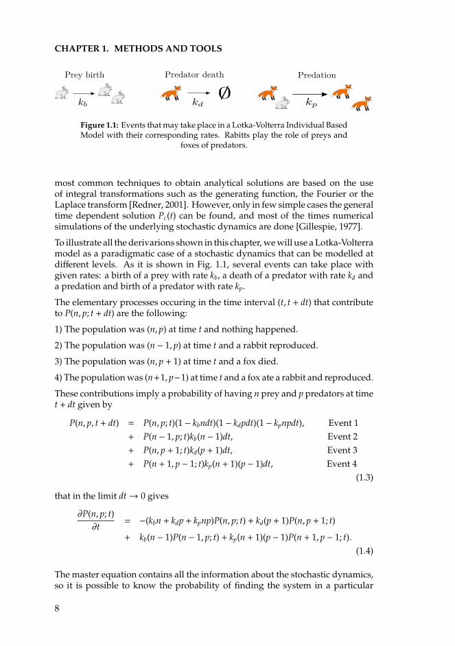
Prey birth Predator death Predation
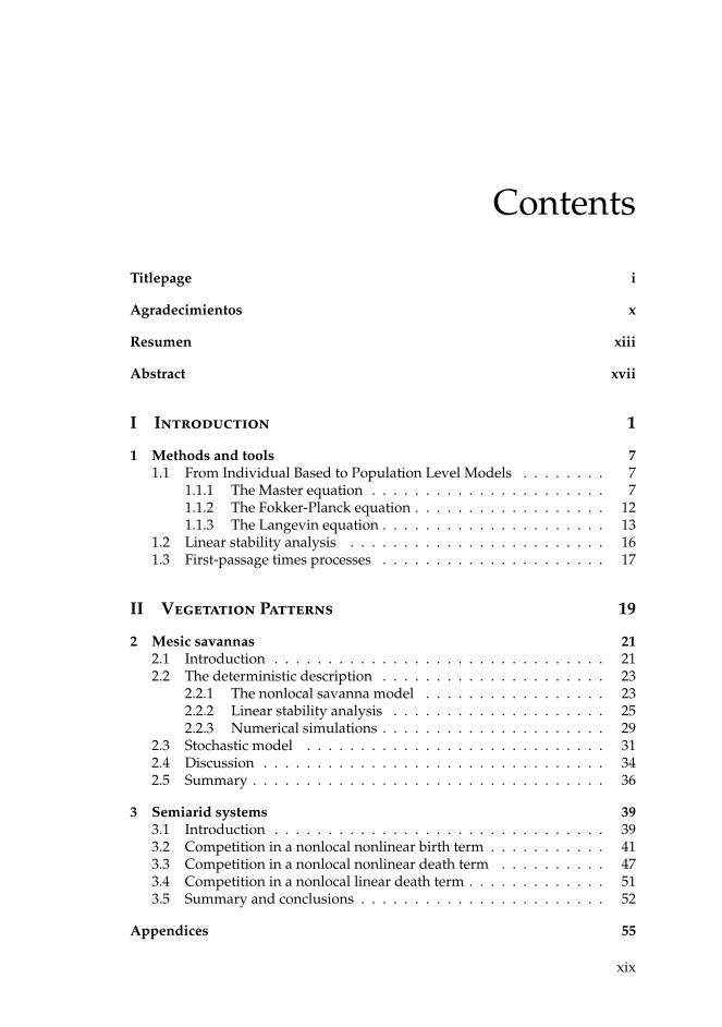
Figure 1.1: Events that may take place in a Lotka-Volterra Individual BasedModel with their corresponding rates. Rabitts play the role of preys and
foxes of predators.
most common techniques to obtain analytical solutions are based on the useof integral transformations such as the generating function, the Fourier or theLaplace transform [Redner, 2001]. However, only in few simple cases the generaltime dependent solution Pc(t) can be found, and most of the times numericalsimulations of the underlying stochastic dynamics are done [Gillespie, 1977].
To illustrate all the derivarions shown in this chapter, we will use a Lotka-Volterramodel as a paradigmatic case of a stochastic dynamics that can be modelled atdifferent levels. As it is shown in Fig. 1.1, several events can take place withgiven rates: a birth of a prey with rate kb, a death of a predator with rate kd anda predation and birth of a predator with rate kp.
The elementary processes occuring in the time interval (t, t + dt) that contributeto P(n, p; t + dt) are the following:
1) The population was (n, p) at time t and nothing happened.
2) The population was (n − 1, p) at time t and a rabbit reproduced.
3) The population was (n, p + 1) at time t and a fox died.
4) The population was (n+1, p−1) at time t and a fox ate a rabbit and reproduced.
These contributions imply a probability of having n prey and p predators at timet + dt given by
P(n, p, t + dt) = P(n, p; t)(1 − kbndt)(1 − kdpdt)(1 − kpnpdt), Event 1+ P(n − 1, p; t)kb(n − 1)dt, Event 2+ P(n, p + 1; t)kd(p + 1)dt, Event 3+ P(n + 1, p − 1; t)kp(n + 1)(p − 1)dt, Event 4
(1.3)
that in the limit dt→ 0 gives
∂P(n, p; t)∂t
= −(kbn + kdp + kpnp)P(n, p; t) + kd(p + 1)P(n, p + 1; t)
+ kb(n − 1)P(n − 1, p; t) + kp(n + 1)(p − 1)P(n + 1, p − 1; t).(1.4)
The master equation contains all the information about the stochastic dynamics,so it is possible to know the probability of finding the system in a particular
8
1.1. FROM INDIVIDUAL BASED TO POPULATION LEVEL MODELS
state as a function of time. However, due to the difficulties that one usuallyfinds to obtain its complete solution, many numerical techniques and analyticalapproximations have been developed to deal with it. This is the case of theGillespie algorithm and the mean-field approximation, that will be explainednext.
The Gillespie algorithm
The Gillespie algorithm [Gillespie, 1977] is a Monte Carlo method used to sim-ulate stochastic processes where transitions from one state to another take placewith different rates. The main objective of the algorithm is to calculate the timeuntil the next transition takes place and the state where the system will moveto. In principle, one should obtain the time at which every transition occurs,then select the one that happens first and execute it. The advantage of Gillespiemethod is that it avoids simulating all the transitions and, instead, only the onethat takes place first has to be reproduced.
The algorithm can be explained in four steps:
1. Considering that the system is initially in one of the possible M states, weobtain the total escape rate from it
Ωi =∑j,i
ωi→ j, i = 1, . . . ,M (1.5)
where j is the set of accesible states from i and ωi→ j are the individualtransition rates from i to each of the states labelled by j.
2. The time until the next jump, dt, is computed. It is drawn from an ex-ponential distribution of mean 1/Ωi. To this aim one generates a randomnumber uniformly distributed, u0, and computes dt as
dt =−lnu0
Ωi. (1.6)
3. The final state has to be determined. Each of the possible transitions takesplace with a probability pi→ j that is proportional to the corresponding rateωi→ j,
pi→ j =ωi→ j
Ωi(1.7)
4. The time is updated t→ t + dt
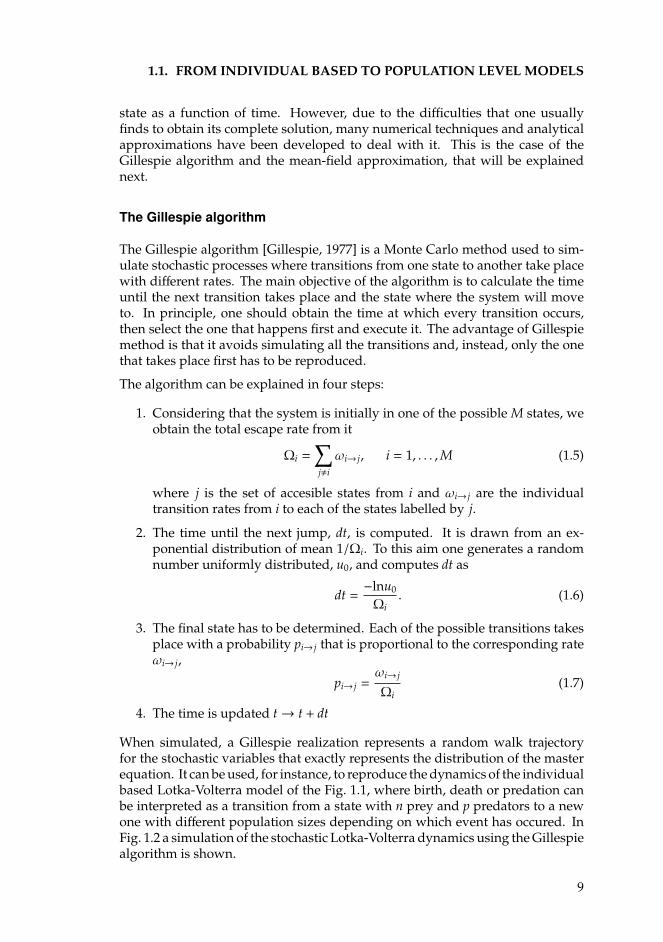
When simulated, a Gillespie realization represents a random walk trajectoryfor the stochastic variables that exactly represents the distribution of the masterequation. It can be used, for instance, to reproduce the dynamics of the individualbased Lotka-Volterra model of the Fig. 1.1, where birth, death or predation canbe interpreted as a transition from a state with n prey and p predators to a newone with different population sizes depending on which event has occured. InFig. 1.2 a simulation of the stochastic Lotka-Volterra dynamics using the Gillespiealgorithm is shown.
9
CHAPTER 1. METHODS AND TOOLS
0 50 100 150 200t
0
100
200
300
Figure 1.2: Evolution of the population of preys (red line) and predators(blue line) from numerical simulations of the stochastic dynamics in Fig. 1.1using Gillespie algorithm. Initial condition 100 preys (rabbits) and 100
predators (foxes)
Mean-field approximation
It is the simplest analytical approximation to deal with a master equation. Itallows the derivation of deterministic differential equations for the mean valuesof the stochastic variables and establishes the simplest class of population-levelmodels. Referring to the Lotka-Volterra model as a guiding example, we willderive the equations for the evolution of the mean number of preys, n, andpredators, p. Given a multivariate probability density function with discretevariables, as it is P(n, p; t), the expected values are defined as
〈n(t)〉 =∞∑
p,n=0
nP(n, p; t), 〈p(t)〉 =∞∑
p,n=0
pP(n, p; t). (1.8)
Multiplying the master equartion, Eq. (1.4), by n and p respectively and makingthe summation over both variables, one gets the equations for the temporalevolution of the mean values coupled to the higher moments 〈n(t)p(t) >
ddt〈n(t)〉 = kb〈n(t)〉 − kp〈n(t)p(t)〉
ddt〈p(t)〉 = kp〈n(t)p(t)〉 − kd〈p(t)〉. (1.9)
It is possible to obtain the equation for the temporal evolution of 〈n(t)p(t)〉, but itwould be again coupled to higher moments, leading to an infinite system of cou-pled differential equations. The main assumption of the mean-field approxima-tion is to consider that both populations are independent, 〈n(t)p(t)〉 = 〈n(t)〉〈p(t)〉,so it is possible to write a closed system of deterministic differential equationsfor the mean value of preys and predators
dNdt
= N(kb − kpP),
dPdt
= P(kpN − kd), (1.10)
10
1.1. FROM INDIVIDUAL BASED TO POPULATION LEVEL MODELS
0 5 10 15 20 25 300.0
0.5
1.0
1.5
2.0
2.5
x
Figure 1.3: Numerical solutions of the nondiemsional Lotka-Volterra equa-tions (1.12) with an initial condition u(0) = 1 and v(0) = 2. α = 1. Thered-dashed line corresponds to the evolution of preys and the blue-full line
to predators.
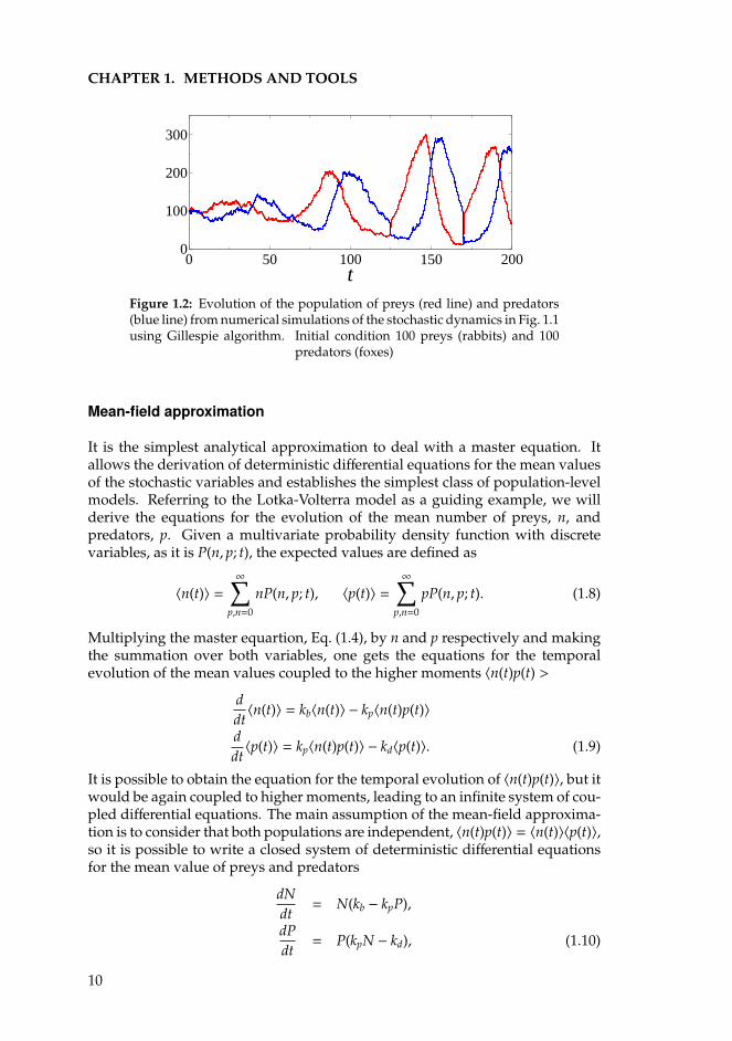
where N(t) ≡ 〈n(t)〉 and P(t) ≡ 〈p(t)〉.For simplicity, the set of equations (1.10) can be nondimensionalised by writing[Murray, 2002]
u(τ) =kpNkd, v(τ) =
kpPkb, τ = kbt, α =
kd
kb, (1.11)
and it becomes,
dudt= u(1 − v),
dvdt= αv(u − 1). (1.12)
The nondimensional system (1.12) can be solved analytically, although this is notthe general case for nonlinear systems. Most of the times one has to use linearapproximations and other techniques developed in the study of dynamical sys-tems. Additionally, it is always possible to numerically integrate the equations.This has been done for equations (1.12) and the results are shown in Fig. 1.3.
The mean-field equations are a simplified version of the complete stochasticdynamics, but still contain most of the relevant information of the system. Forinstance, the oscillations in the populations are preserved for the Lotka-Volterramodel. However, there are many other approximations that, although morecomplicated, are able to keep the inherent stochasticity of the system. TheFokker-Planck and the Langevin equations are two of them.
11
CHAPTER 1. METHODS AND TOOLS
1.1.2 The Fokker-Planck equation
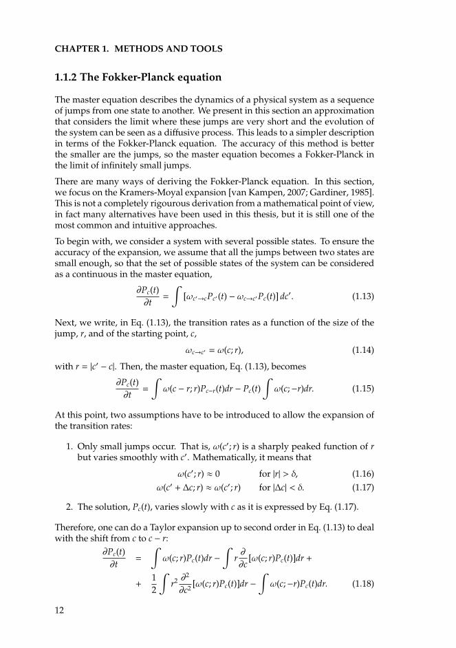
The master equation describes the dynamics of a physical system as a sequenceof jumps from one state to another. We present in this section an approximationthat considers the limit where these jumps are very short and the evolution ofthe system can be seen as a diffusive process. This leads to a simpler descriptionin terms of the Fokker-Planck equation. The accuracy of this method is betterthe smaller are the jumps, so the master equation becomes a Fokker-Planck inthe limit of infinitely small jumps.
There are many ways of deriving the Fokker-Planck equation. In this section,we focus on the Kramers-Moyal expansion [van Kampen, 2007; Gardiner, 1985].This is not a completely rigourous derivation from a mathematical point of view,in fact many alternatives have been used in this thesis, but it is still one of themost common and intuitive approaches.
To begin with, we consider a system with several possible states. To ensure theaccuracy of the expansion, we assume that all the jumps between two states aresmall enough, so that the set of possible states of the system can be consideredas a continuous in the master equation,
∂Pc(t)∂t
=
∫[ωc′→cPc′(t) − ωc→c′Pc(t)] dc′. (1.13)
Next, we write, in Eq. (1.13), the transition rates as a function of the size of thejump, r, and of the starting point, c,
ωc→c′ = ω(c; r), (1.14)
with r = |c′ − c|. Then, the master equation, Eq. (1.13), becomes
∂Pc(t)∂t
=
∫ω(c − r; r)Pc−r(t)dr − Pc(t)
∫ω(c;−r)dr. (1.15)
At this point, two assumptions have to be introduced to allow the expansion ofthe transition rates:
1. Only small jumps occur. That is, ω(c′; r) is a sharply peaked function of rbut varies smoothly with c′. Mathematically, it means that
ω(c′; r) ≈ 0 for |r| > δ, (1.16)ω(c′ + ∆c; r) ≈ ω(c′; r) for |∆c| < δ. (1.17)
2. The solution, Pc(t), varies slowly with c as it is expressed by Eq. (1.17).
Therefore, one can do a Taylor expansion up to second order in Eq. (1.13) to dealwith the shift from c to c − r:
∂Pc(t)∂t
=
∫ω(c; r)Pc(t)dr −
∫r∂
∂c[ω(c; r)Pc(t)]dr +
+12
∫r2 ∂
2
∂c2 [ω(c; r)Pc(t)]dr −∫ω(c;−r)Pc(t)dr. (1.18)
12
1.1. FROM INDIVIDUAL BASED TO POPULATION LEVEL MODELS
The first and fourth term in the right-hand side of Eq. (1.18) cancel each other,and defining the jump moments
αν(c) =∫ +∞
−∞rνω(c; r)dr, (1.19)
the final result can be written as
∂Pc(t)∂t
= − ∂∂c
[α1(c)Pc(t)] +12∂2
∂c2 [α2(c)Pc(t)]. (1.20)
This is the Fokker-Planck equation. It is important to remark that we have notshown a completely rigurous derivation. The election of the small parameter toperform the Taylor expansion has not been justified and there are many processesin which this expansion fails. This is the case of systems with jump size ±1 orsome small integer, whereas typical sizes of the variable may be large, e.g., thenumber of molecules in a chemical reaction or the position of a random walker ona long lattice. In those cases expansions where the small parameter is explicitlytaken are much more appropiate (See Chapter 6 for a rigorous derivation of theFokker-Planck equation). Nevertheless, this description provides a good firstcontact with the Fokker-Planck equation, that allows the development of a largevariety of population level spatial models.
On the other hand, many ecological systems, such as groups of animals andvegetation landscapes that will be studied in this thesis, are formed by manyparticles. Let us now suppose that we have a suspension of a very large numberof identical individuals, and denote its local density by ρ(x, t). If the suspensionis sufficiently diluted, to the extent that particles can be considered independent,then ρ(x, t) will obey the same Eq. (1.20) [Peliti, 2011]. This family of modelsbased on the density of individuals is the basis of the studies on vegetationpatterns shown in the Part II of this thesis.
In either case, and independently of the way used to write it, the Fokker-Planckequation describes a large class of stochastic dynamics in which the system hasa continuous sample path. The state of the system can be written as a stochasticand continuous function of time. From this picture, it seems obvious to seek adescription in some direct probabilistic way and in terms of stochastic differentialequations for the path of the system. This procedure is discused next.
1.1.3 The Langevin equation
In some cases it is useful to describe a system in terms of a differential equation,that gives the stochastic evolution of its state as a trajectory in the phase space.This is the Langevin equation, that has the general form
dcdt= f (c, t) + g(c, t)η(t), (1.21)
where c is a stochastic variable that gives the state of the system at every time.f (c, t) and g(c, t) are known functions and η(t) is a rapidly fluctuating term whose
13
CHAPTER 1. METHODS AND TOOLS
average over single realizations is equal to zero, 〈η(t)〉 = 0. Any nonzero meancan be absorbed into the definition of f (c, t). An idealization of a term like η(t)must be that in which if t , t′, η(t) and η(t′) are statistically independent (whitenoise), so
〈η(t)η(t′)〉 = Γδ(t − t′), (1.22)
where Γ gives the strength of the random function.
To be rigorous, the differential equation (1.21) is not properly defined, althoughthe corresponding integral equation,
c(t) − c(0) =∫ t
0f [c(s), s]ds +
∫ t
0g[c(s), s]η(s)ds, (1.23)
can be consistently defined understanding the integral of the white noise as aWiener process W(t) [van Kampen, 2007; Gardiner, 1985]:
dW(t) ≡W(t + dt) −W(t) = η(t)dt. (1.24)
Hence
c(t) − c(0) =∫ t
0f [c(s), s]ds +
∫ t
0g[c(s), s]dW(s), (1.25)
where the second integral can be seen like a kind of Riemann integral withrespect to a sample function W(t).
The definition of the Langevin equation (1.21), requires a careful interpretationdue to this lack of mathematical rigor. When the noise term appears multiplica-tively, that is, g(c, t) is not a constant, ambiguities appear in some mathematicalexpressions. Giving a sense to the undefined expressions constitutes one of themain goals when integrating a Langevin equation. The most widely used in-terpretations are those of Ito and Stratonovich (Appendix F). The Ito integral ispreferred by mathematicians [van Kampen, 2007], but it is not always the mostnatural choice from a physical point of view. The Stratonovich integral is moresuitable, for instance, when η(t) is a real noise with finite correlation time wherethe vanishing correlation time limit wants to be taken. (In the Appendix F weshow a more detailed discussion). The matter is not what is the right definitionof the stochastic integral, but how stochastic processes can model real systems.That is, in what situations either Ito or Stratonovich choice is the most suitable.
Langevin equations are also valid to go beyond a mean-field description. Inthese cases a new term enters in the equation to include diffusion, besides otherspatial couplings and degrees of freedom. The variable c(t) becomes a continuousfield φ(r, t) that depends on space and time. The Langevin equation becomes astochastic partial differential equation of the type
∂φ(r, t)∂t
= f (φ(r, t), t) + ∇2φ(r, t) + g(φ(r, t), t)η(r, t). (1.26)
This approach is quite useful for spatially extended systems or to study theformation of patterns.
14
1.1. FROM INDIVIDUAL BASED TO POPULATION LEVEL MODELS
From the Fokker-Planck to Langevin equation and vice versa.
To close this overview on the modeling of stochastic systems, we will show therelationship between Fokker-Planck and Langevin equations. Starting from aFokker-Planck equation for the probability distribution of the variable c
∂P(c, t)∂t
= − ∂∂cα1(c)P(c, t) +
12∂2
∂c2α2(c)P(c, t), (1.27)
it is easy to write down a Langevin equation of the type (1.21) [Gardiner, 1985;van Kampen, 2007]
dcdt= f (c, t) + g(c, t)η(t), (1.28)
where η(t) is a white, Gaussian and zero mean noise.
The coefficients of the equations are related according to
f (c, t) = α1(c, t), (1.29)
g(c, t) =√α2(c, t). (1.30)
provided that the Ito interpretation is chosen.
The first term in Eq. (1.27) is called drift, because it leads to the deterministicpart of the Langevin equation, and the second one, the diffusion term, since itdetermines the stochastic part of the Langevin equation.
In the Stratonovich scheme an additional drift appears,
dcdt= f (c, t) +
12
g(c, t)∂g(c, t)∂c
+ g(c, t)η(t). (1.31)
On the other hand, if the starting point is a Langevin equation
dcdt= f (c, t) + g(c, t)η(t), (1.32)
to obtain the Fokker-Planck equation one has to specify if the Ito or the Stratonovichcalculus will be used. In the Stratonovich interpretation the Fokker-Planck is
∂P(c, t)∂t
= − ∂∂c
f (c)P(c, t) +12∂
∂cg(c)
∂
∂cg(c)P(c, t), (1.33)
while in the Ito case it is∂P(c, t)∂t
= − ∂∂c
f (c)P(c, t) +12∂2
∂c2 [g(c)]2P(c, t). (1.34)
The diffusion term vanishes typically with the number of components as N−1/2,so it is negligible if the system is large enough. Therefore, in the thermodynamiclimit where N and the volume V tend to infinity keeping N/V finite, a determin-istic mean-field approximation gives an accurate description. Sometimes, thisway is walked on the inverse sense. One may start with a deterministic equa-tion and, using heuristic arguments, add noise to obtain the Langevin equation.Then, following the steps that have been explained in this section it is possibleto get a Fokker-Planck equation.
15
CHAPTER 1. METHODS AND TOOLS
1.2
Linear stability analysis
Linear stability analysis is the simplest analytical tool used to study the forma-tion of patterns in deterministic spatially extended systems. It assumes an idealinfinite system and uses Fourier analysis to investigate the stability of its homo-geneous state. We will consider in this section the two dimensional case. Thestarting point is the equation for the evolution of a field φ
∂φ(x, y, t)∂t
= f(φ(x, y, t),
∂φ
∂x,∂φ
∂y,∂2φ
∂x2 ,∂2φ
∂y2 ,∂2φ
∂x∂y; R
)(1.35)
where R is the control parameter. The linear stability analysis assumes that thesystem is at the homogeneous (spatially independent) stationary stateφ(x, t) = φ0and studies its stability against small perturbations that will be denoted byψ(x, t),with |ψ| 1. The technique is applied in the Appendix A to one particular caseand the calculations explained in detail. In this section we will introduce anddiscuss the theoretical basis and the main results that can be obtained. Pluggingthe ansatz φ(x, t) = φ0 +ψ(x, t) into the model Eq. (1.35) and retaining only linearterms in the perturbation, one obtains a linear equation for the evolution ofthe perturbation at short times that can be solved using the Fourier transform.Then, the final task is to solve the transformed equation for the perturbation,ψ(k, t). Assuming that at short time scales the temporal dependence is ψ(k, t) ∝exp(λ(k)), where λ is the growth rate, then ψ(k, t) = λ(k)ψ(k, t). Finally anexpression for λ(k) can be obtained. It is called the dispersion relation andcontains all the information about the evolution of the Fourier modes of ψ(k, t).The modes k with a negative growth rate will be stable while those correspondingto λ ≥ 0 are unstable and lead to perturbations growing in time and, therefore, tospatial patterns in the system. The dispersion relation also allows to obtain thecharacteristic wavelength of the pattern through the value of the most unstableFourier mode, kc, that most of the times corresponds with the one with thehighest growth rate.
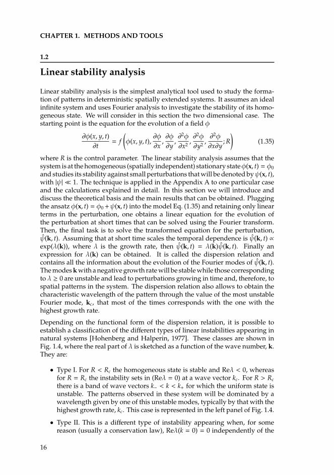
Depending on the functional form of the dispersion relation, it is possible toestablish a classification of the different types of linear instabilities appearing innatural systems [Hohenberg and Halperin, 1977]. These classes are shown inFig. 1.4, where the real part of λ is sketched as a function of the wave number, k.They are:
• Type I. For R < Rc the homogeneous state is stable and Reλ < 0, whereasfor R = Rc the instability sets in (Reλ = 0) at a wave vector kc. For R > Rcthere is a band of wave vectors k− < k < k+ for which the uniform state isunstable. The patterns observed in these system will be dominated by awavelength given by one of this unstable modes, typically by that with thehighest growth rate, kc. This case is represented in the left panel of Fig. 1.4.
• Type II. This is a different type of instability appearing when, for somereason (usually a conservation law), Reλ(k = 0) = 0 independently of the
16

1.3. FIRST-PASSAGE TIMES PROCESSES
kc
Reλ
k k k
R < Rc
R = Rc
R > Rc
I II III
k−
k+ k+
Figure 1.4: Different types of linear instabilities depicted in the real part ofthe dispersion relation.
value of the control parameter R. This corresponds with the central panelof Fig. 1.4. The critical wave vector, the one that becomes unstable by thefirst time, is now kc = 0, and a band of unstable modes appears between 0and k+ for R > Rc. The pattern occurs on a long length scale. This case isremarkable because the critical wave vector is different from that with thehighest growth rate.
• Type III. In this case both the instability and the maximum growth rateoccur at kc = 0. There is not an intrinsic length scale, and patterns willoccur over a length scale defined by the system size or the dynamics. Thissituation is depicted in the right panel of Fig. 1.4.
Finally, there are two subtypes for each type of instability depending on thetemporal instability: stationary if Imλ = 0, and oscillatory if Imλ , 0.
Linear stability analysis provides analytical results about the formation of pat-terns in spatially extended systems, such as the dominant wavelength and thetype of instability leading the structure. However, it is important to remark thatthe analysis assumes that the perturbations of the uniform state are small. Thisassumption is good at short times and for an initial condition that has a smallmagnitude, but at long times the nonlinear terms left out in the linear approxima-tion become important [Cross and Greenside, 2009]. One effect of nonlinearityis to quench the assumed exponential growth. Further analysis, such as weaklynonlinear stability analysis [Cross and Hohenberg, 1993], must be used in thesecases.
1.3
First-passage times processes
First-passage phenomena are of high relevance in stochastic processes that aretriggered by a first-passage event [Redner, 2001] and play a fundamental role
17
CHAPTER 1. METHODS AND TOOLS
quantifying and limiting the success of different processes that can be mappedinto random walks. Ecology and biology offer some examples such as the lifetimeof a population or the duration of a search or a biochemical reaction.
In this section we will present some results on first-passage times in the simplecase of a discrete symmetric random walk moving in a finite interval [x−, x+][Redner, 2001]. The extension to higher dimensions is straightforward. Let usdenote the mean time to exit the interval starting at x by T(x). This quantityis equal to the exit time of a given trajectory times the probability of that path,averaged over all the trajectories,
T(x) =∑
p
Pptp(x), (1.36)
where tp is the exit time of the trajectory p that starts at x and Pp the probabilityof the path. Because of the definition of a symmetric random walk on a discretespace, the mean exit time also obeys
T(x) =12[T(x + δx) + δt] + [T(x − δx) + δt] , (1.37)
with boundary conditions T(x−) = T(x+) = 0 which correspond to a mean exittime equal to zero if the particle starts at either border of the interval. δx is thejumping length. This recursion relation expresses the mean exit time starting atx in terms of the outcome one step in the future, for which the initial walk canbe seen as restarting in x ± δx (each with probability 1/2) but also with the timeincremented by δt.
Doing a Taylor expansion to the lowest nonvanishing order in Eq. (1.37), andconsidering the limit of continuous time and space, it yields
Dd2Tdx2 = −1, (1.38)
where D = δx2/2δt is the difussion constant. In the case of a two dimensionaldomain Eq. (1.38) is
D∇2T(x) = −1. (1.39)
These results can be extended to the case of general jumping processes with asingle-step jumping probability given by px→x′ . The equivalent of Eq. (1.37) is
T(x) =∑
x′px→x′[T(x′) + δt], (1.40)
that provides an analog of Eq. (1.39) that is
D∇2T(x) + v(x) ·∇T(x) = −1, (1.41)
where v(x) is a local velocity that gives the mean displacement after a single stepwhen starting from x in the hopping process. This equation can be solved ineach particular case. We have used it in this thesis as an starting point of manyof the calculations in the Part IV. See Appendix G for a detailed calculation.
18
Part II
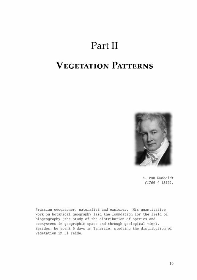
Vegetation Patterns
A. von Humboldt
(1769 1859).
Prussian geographer, naturalist and explorer. His quantitative
work on botanical geography laid the foundation for the field of
biogeography (the study of the distribution of species and
ecosystems in geographic space and through geological time).
Besides, he spent 6 days in Tenerife, studying the distribution of
vegetation in El Teide.
19

CHAPTER 2Mesic savannas
In this chapter we propose a continuum description for the dynamics of treedensity in mesic savannas inspired on the individual based model introduced inCalabrese et al. [2010]. It considers only long-range competition among trees andthe effect of fires resulting in a local facilitation mechanism. Despite short-rangefacilitation is taken to the local-range limit, the standard full spectrum of spatialstructures obtained in general vegetation models is recovered. Long-range com-petition is thus the key ingredient for the development of patterns. This resultopens new questions on the role that facilitative interactions play in the mainte-nance of vegetation patterns. The long time coexistence between trees and grass,the effect of fires on the survival of trees as well as the maintenance of the patternsare also studied. The influence of demographic noise is analyzed. The stochasticsystem, under parameter constraints typical of more humid landscapes, showsirregular patterns characteristic of realistic situations. The coexistence of treesand grass still remains at reasonable noise intensities.
2.1
Introduction
Savanna ecosystems are characterized by the long-term coexistence between acontinuous grass layer and scattered or clustered trees [Sarmiento, 1984]. Oc-curring in many regions of the world, in areas with very different climatic andecological conditions, the spatial structure, persistence, and resilience of sa-vannas have long intrigued ecologists [Scholes and Archer, 1997; Sankaran et al.,2005; Borgogno et al., 2009; Belsky, 1994]. However, despite substantial research,the origin and nature of savannas have not yet been fully resolved and muchremains to be learned.
Savanna tree populations often exhibit pronounced, non-random spatial struc-tures [Skarpe, 1991; Barot et al., 1999; Jeltsch et al., 1999; Caylor et al., 2003;Scanlon et al., 2007]. Much research has therefore focused on explaining howspatial patterning in savannas arises [Jeltsch et al., 1996, 1999; Scanlon et al., 2007;
21
CHAPTER 2. MESIC SAVANNAS
Skarpe, 1991; Calabrese et al., 2010; Vazquez et al., 2010]. In most natural plantsystems both facilitative and competitive processes are simultaneously present[Scholes and Archer, 1997; Vetaas, 1992] and hard to disentangle [Veblen, 2008;Barbier et al., 2008]. Some studies have pointed toward the existence of short-distance facilitation [Caylor et al., 2003; Scanlon et al., 2007], while others havedemonstrated evidence of competition [Skarpe, 1991; Jeltsch et al., 1999; Barotet al., 1999], with conflicting reports sometimes arriving from the same regions.
Different classes of savannas, which can be characterized by how much rainfallthey typically receive, should be affected by different sets of processes. Forexample, in semiarid savannas water is extremely limited (low mean annualprecipitation) and competition among trees is expected to be strong, but fire playslittle role because there is typically not enough grass biomass to serve as fuel.In contrast, humid savannas should be characterized by weaker competitionamong trees, but also by frequent and intense fires. In-between these extremes,in mesic savannas, trees likely have to contend with intermediate levels of bothcompetition for water and fire [Calabrese et al., 2010; Sankaran et al., 2005, 2008;Bond et al., 2003; Bond, 2008; Bucini and Hanan, 2007].
Competition among trees is mediated by roots that typically extend well beyondthe crown [Borgogno et al., 2009; Barbier et al., 2008]. Additionally, fire can leadto local facilitation due to a protection effect, whereby vulnerable juvenile treesplaced near adults are protected from fire by them [Holdo, 2005]. We are par-ticularly interested in how the interplay between these mechanisms governs thespatial arrangement of trees in mesic savannas, where both mechanisms may op-erate. On the other side, it has frequently been claimed that pattern formation inarid systems can be explained by a combination of long-distance competition andshort-distance facilitation [Klausmeier, 1999; Lefever and Lejeune, 1997; Lefeveret al., 2009; Lefever and Turner, 2012; Rietkerk et al., 2002; von Hardenberg et al.,2001; D’Odorico et al., 2006b]. This combination of mechanisms is also known toproduce spatial structures in many other natural systems [Cross and Hohenberg,1993]. Although mesic savannas do not display the same range of highly regularspatial patterns that arise in arid systems (e.g., tigerbush), similar mechanismsmight be at work. Specifically, the interaction between long-range competitionand short-range facilitation might still play a role in pattern formation in savannatree populations, but only for a limited range of parameter values and possiblymodified by demographic stochasticity.
Although the facilitation component has often been thought to be a key com-ponent in previous vegetation models [D’Odorico et al., 2006b,c; Rietkerk et al.,2002; Scanlon et al., 2007], Rietkerk and Van de Koppel [Rietkerk and van deKoppel, 2008], speculated, but did not show, that pattern formation could oc-cur without short-range facilitation in the particular example of tidal freshwatermarsh. In the case of savannas, as stated before, the presence of adult trees favorthe establishment of new trees in the area, protecting the juveniles against fires.Considering this effect, we take the facilitation component to its infinitesimallyshort spatial limit, and study its effect in the emergence of spatially periodicstructures of trees. To our knowledge, this explanation, and the interrelation
22
2.2. THE DETERMINISTIC DESCRIPTION
between long-range competition and local facilitation, has not been explored fora vegetation system.
To this aim, we develop a minimalistic model of savannas that considers two ofthe factors, as already mentioned, thought to be crucial to structure mesic savan-nas: tree-tree competition and fire, with a primary focus on spatially nonlocalcompetition. Employing standard tools used in the study of pattern formationphenomena in physics (stability analysis and the structure function) [Cross andHohenberg, 1993], we explore the conditions under which the model can pro-duce non-homogeneous spatial distributions. A key strength of our approach isthat we are able to provide a complete and rigorous analysis of the patterns themodel is capable of producing, and we identify which among these correspondto situations that are relevant for mesic savannas. We further examine the role ofdemographic stochasticity in modifying both spatial patterns and the conditionsunder which trees persist in the system in the presence of fire, and discuss theimplications of these results for the debate on whether the balance of processesaffecting savanna trees is positive, negative, or is variable among systems. This isthe framework of our study: the role of long-range competition, local facilitationand demographic fluctuations in the spatial structures of mesic savannas.
2.2
The deterministic description
In this section we derive the deterministic equation for the local density oftrees, such that dynamics is of the logistic type and we only consider tree-treecompetition and fire. We study the formation of patterns via stability analysisand provide numerical simulations, showing the emergence of spatial structures.
2.2.1 The nonlocal savanna model
Calabrese et al. [2010] introduced a simple discrete-particle lattice savanna modelthat considers the birth-death dynamics of trees, and where tree-tree competitionand fire are the principal ingredients. These mechanisms act on the probabilityof establishment of a tree once a seed lands at a particular point on the lattice. Inthe discrete model, seeds land in the neighborhood of a parent tree with a rateb, and establish as adult trees if they are able to survive both competition neigh-boring trees and fire. As these two phenomena are independent, the probabilityof establishment is PE = PCPF, where PC is the probability of surviving the com-petition, and PF is the probability of surviving a fire event. From this dynamics,we write a deterministic differential equation describing the time evolution ofthe global density of trees (mean field), ρ(t), where the population has logisticgrowth at rate b, and an exponential death term at rate α. It reads:
dρdt= bPE(ρ)ρ(t)
(1 − ρ(t)
) − αρ(t). (2.1)
23
CHAPTER 2. MESIC SAVANNAS
Generalizing Eq. (2.1), we propose an evolution equation for the space-dependent(local) density of trees, ρ(x, t):
∂ρ(x, t)∂t
= bPEρ(x, t)(1 − ρ(x, t)) − αρ(x, t). (2.2)
We allow the probability of overcoming competition to depend on tree crowdingin a local neighborhood, decaying exponentially with the density of surroundingtrees as
PC = exp(−δ
∫G(x − r)ρ(r, t)dr
), (2.3)
where δ is a parameter that modulates the strength of the competition, and G(x)is a positive kernel function that introduces a finite range of influence. Thismodel is related to earlier one of pattern formation in arid systems [Lefever andLejeune, 1997], and subsequent works [Lefever et al., 2009; Lefever and Turner,2012], but it differs from standard kernel-based models in that the kernel functionaccounts for the interaction neighborhood, and not for the type of interactionwith the distance. Note also that the nonlocal term enters nonlinearly in theequation.
Following Calabrese et al. [2010], PF is assumed to be a saturating function ofgrass biomass, 1 − ρ(x, t), similar to the implementation of fire of Jeltsch et al. in[Jeltsch et al., 1996]
PF =σ
σ + 1 − ρ(x, t), (2.4)
where σ governs the resistance to fire, so σ = 0 means no resistance to fires.Notice how our model is close to the one in [Calabrese et al., 2010] through thedefinitions of PC and PF, although we consider the probability of surviving a firedepending on the local density of trees, and in [Calabrese et al., 2010] it dependson the global density. The final deterministic differential equation that considerstree-tree competition and fire for the spatial tree density is
∂ρ(x, t)∂t
= be f f (ρ)ρ(x, t)(1 − ρ(x, t)
) − αρ(x, t), (2.5)
where
be f f (ρ) =be−δ
∫G(x−r)ρ(r,t)drσ
σ + 1 − ρ(x, t). (2.6)
Thus, we have a logistic-type equation with an effective growth rate that de-pends nonlocally on the density itself, and which is a combination of long-rangecompetition and local facilitation mechanisms (fire). The probability of surviv-ing a fire is higher when the local density of trees is higher, as can be seen fromthe definition in Eq. (refprobfire).
In Fig. 2.1 we show numerical solutions for the mean field Eq. (refeq:mf) (lines)and the spatially explicit model (equation 2.5) (dots) in the stationary state (t→∞) using different values of the competition. We have used a top-hat function asthe competition kernel, G(x) (See Sec. 2.2.2 for more details on the kernel choice).
24
2.2. THE DETERMINISTIC DESCRIPTION
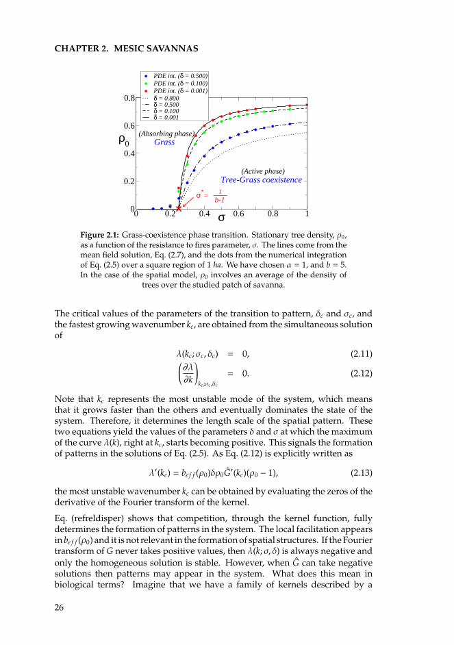
We observe a very good agreement of both descriptions which becomes worsewhen we get closer to the critical point σ∗, where the model presents a phasetransition from a tree-grass coexistence to a grassland state. This disagreementappears because while the mean field equation describes an infinite system, theEq. (2.5) description forces us to choose a size for the system.
The model reproduces the long-term coexistence between grass and trees thatis characteristic of savannas. To explore this coexistence, we study the long-time behavior of the system and analyze the homogeneous stationary solutionsof Eq. (2.5), which has two fixed points. The first one is the absorbing staterepresenting the absence of trees, ρ0 = 0, and the other can be obtained, in thegeneral case, by numerically solving
be f f (ρ0)(1 − ρ0) − α = 0. (2.7)
In the regime where ρ0 is small (near the critical point), if competition intensity,δ, is also small, it is possible to obtain an analytical expression for the criticalvalue of the probability of surviving a fire, σ∗,
σ∗ =α
b − α. (2.8)
Outside of the limit where δ 1, we can solve Eq. (2.7) numerically in ρ0 to showthat the critical value of the fire resistance parameter, σ∗, does not depend oncompetition. A steady state with trees is stable for higher fire survival probability(Fig. 2.1).
There is, then, a transition from a state where grass is the only form of vegetationto another state where trees and grass coexist at σ∗. In what follows, we fix α = 1,so we choose our temporal scale in such a way that time is measured in units ofα. This choice does not qualitatively affect our results.
2.2.2 Linear stability analysis
The spatial patterns can be studied by performing a linear stability analysis[Cross and Hohenberg, 1993] of the stationary homogeneous solutions of Eq. (ref-sav1), ρ0 = ρ0(σ, δ). The stability analysis is performed by considering smallharmonic perturbations around ρ0, ρ(x, t) = ρ0 + εeλt−ik · x, ε 1. After somecalculations1, one arrives at a perturbation growth rate given by
λ(k; σ, δ) = be f f
(ρ0)1 + σ(1 − 2ρ0)σ − ρ0 + 1
−ρ0
[2 − ρ0 + δG(k)(ρ0 − 1)(ρ0 − 1 − σ)
](σ − ρ0 + 1)
− 1,
(2.9)where G(k), k = |k|, is the Fourier transform of the kernel,
G(k) =∫
G(x)e−ik · xdx. (2.10)
1A linear stability analysis in a similar equation modeling vegetation in arid systems is shownin detail in Appendix A.
25
CHAPTER 2. MESIC SAVANNAS
0 0.2 0.4 0.6 0.8 1σ0
0.2
0.4
0.6
0.8
ρ0
PDE int. (δ = 0.500)PDE int. (δ = 0.100)PDE int. (δ = 0.001)δ = 0.800δ = 0.500δ = 0.100δ = 0.001
Tree-Grass coexistence
Grass
(Active phase)
(Absorbing phase)
σ*= 1
b-1
Figure 2.1: Grass-coexistence phase transition. Stationary tree density, ρ0,as a function of the resistance to fires parameter, σ. The lines come from themean field solution, Eq. (2.7), and the dots from the numerical integrationof Eq. (2.5) over a square region of 1 ha. We have chosen α = 1, and b = 5.In the case of the spatial model, ρ0 involves an average of the density of
trees over the studied patch of savanna.
The critical values of the parameters of the transition to pattern, δc and σc, andthe fastest growing wavenumber kc, are obtained from the simultaneous solutionof
λ(kc; σc, δc) = 0, (2.11)(∂λ
∂k
)kc;σc,δc
= 0. (2.12)
Note that kc represents the most unstable mode of the system, which meansthat it grows faster than the others and eventually dominates the state of thesystem. Therefore, it determines the length scale of the spatial pattern. Thesetwo equations yield the values of the parameters δ and σ at which the maximumof the curve λ(k), right at kc, starts becoming positive. This signals the formationof patterns in the solutions of Eq. (2.5). As Eq. (2.12) is explicitly written as
λ′(kc) = be f f (ρ0)δρ0G′(kc)(ρ0 − 1), (2.13)
the most unstable wavenumber kc can be obtained by evaluating the zeros of thederivative of the Fourier transform of the kernel.
Eq. (refreldisper) shows that competition, through the kernel function, fullydetermines the formation of patterns in the system. The local facilitation appearsin be f f (ρ0) and it is not relevant in the formation of spatial structures. If the Fouriertransform of G never takes positive values, then λ(k; σ, δ) is always negative andonly the homogeneous solution is stable. However, when G can take negativesolutions then patterns may appear in the system. What does this mean inbiological terms? Imagine that we have a family of kernels described by a
26
2.2. THE DETERMINISTIC DESCRIPTION
parameter p: G(x) = exp(−|(x)/R|p) (R gives the range of competition). Thekernels are more peaked around x = 0 for p < 2 and more box-like when p > 2.It turns out that this family of functions has non-negative Fourier transform for0 ≤ p < 2, so that no patterns appear in this case. A lengthy discussion of thisproperty in the context of competition of species can be found in Pigolotti et al.[2007]. Thus, the shape of the competition kernel dictates whether or not patternswill appear in the system. If pattern formation is possible, then the values of thefire and competition parameters govern the type of solution (see Sec. 2.2.3).
Our central result for nonlocal competition is that, contrary to conventionalwisdom, it can, in the limit of infinitesimally short (purely local) facilitation,promote the clustering of trees. Whether or not this occurs depends entirely onthe shape of the competition kernel. For large p we have a box-like shape, andin these cases trees compete strongly with other trees, roughly within a distanceR from their position. The mechanism behind this counterintuitive result is thattrees farther than R away from a resident tree area are not able to invade the zonedefined by the radius R around the established tree (their seeds do not establishthere), so that an exclusion zone develops around it. For smaller p there is lesscompetition and the exclusion zones disappear. We will develop longer thisconcept in the next chapter.
For a more detailed analysis, one must choose an explicit form for the kernelfunction. Our choice is determined by the original PC taken in [Calabrese et al.,2010], so that it decays exponentially with the number of trees in a neighborhoodof radius R around a given tree. Thus, for G we take the step function (limitp→∞)
G(|r|) =
1 i f |r| ≤ R
0 i f |r| > R.(2.14)
As noticed before, the idea behind the nonlocal competition is to capture theeffect of the long roots of a tree. The kernel function defines the area of influenceof the roots, and it can be modeled at first order with the constant function ofEq. (refkerneldd). Thus the parameter R, which fixes the nonlocal interactionscale, must be of the order of the length of the roots [Borgogno et al., 2009].Since the roots are the responsible for the adsorption of resources (water andsoil nutrients), a strong long-range competition term implies strong resourcedepletion. For this kernel the Fourier transform is [Lopez and Hernandez-Garcıa, 2004] G(k) = 2πR2J1(kR)/kR and its derivative is G′(k) = −2πR2 J2(kR)/k,where k ≡ |k|, and Ji is the ith-order Bessel function. Since G(k) can take positiveand negative values, pattern solutions may arise in the system, that will inturn depend on the values of δ and σ. The most unstable mode is numericallyobtained as the first zero of λ′(k), Eq. (2.13), which means the first zero of theBessel function J2(kR). This value only depends on R, being independent of theresistance to fires and competition, and it is kc = 5.136/R. Because a pattern of ncells is characterized by a wavenumber kc = 2πn/L, where L is the system size,the typical distance between clusters, dt = L/n, using the definition of the criticalwavenumber is given by dt ≈ 1.22R. In other words, it is approximately the
27
CHAPTER 2. MESIC SAVANNAS
range of interaction R. This result is also independent of the other parameters ofthe system.
Since we are interested in the effect of competition and fire on the distributionof savanna trees, we will try to fix all the parameters but σ and δ. We willexplore the effect of different values of these parameters on the results. First,we have chosen, as in Calabrese et al. [2010], the death rate α = 1, and solvingEq. (2.7) we will roughly estimate the birth rate, b. We will work in the limitof intermediate to high mean annual precipitation, so water is non-limiting andthus we can neglect the effects of competition (δ = 0). At this intermediate tohigh mean annual precipitation the empirically observed upper limit of savannatree cover is approximately ρ0 = 0.8 [Sankaran et al., 2005; Bucini and Hanan,2007]. To reach this upper limit in the tree cover, disturbances must also beabsent, implying no fire (σ → ∞). In this limit, the mean field Eq. (refeq:mf) isquantitatively accurate, as it is shown in Fig. 2.1, and the stationary mean fieldsolution of the model depends only on the birth rate
ρ0(σ→∞) =b − 1
b. (2.15)
It can be solved for b for a fixed ρ0 = 0.8, and it yields b = 5 [Calabrese et al.,2010]. In the following we just consider the dependence of our results on δ andσ. In particular, ρ0 = ρ0(σ, δ).
The phase diagram of the model, computed numerically, is shown in Fig. 2.2,where we plot the spatial character of the steady solution (homogeneous orinhomogeneous) as a function of δ and σ. Note that increasing competitionenhances the inhomogeneous or pattern solution. This is because, as we are nowin the case of a kernel giving rise to clusters, increasing δ makes it more difficultto enter the exclusion zones in-between the clusters. For very strong competition(high, unrealistic, δ), fire has no influence on the pattern.
The critical line separating these two solutions (pattern and homogeneous) canbe obtained analytically as a function of the parameters δ, σ, ρ0 and G(kc). Takingb = 5 and α = 1, it is
σc =(ρ0−1)[5(ρ0−1)(δG(kc)ρ0−1)−2eδπR2ρ0 ]+(ρ0−1)
√5[5(ρ0−1)2(δG(kc)ρ0−1)2−4eδπR2ρ0ρ0
]10
[1−2ρ0+δG(kc)ρ0(1+ρ0)−eδπR2ρ0 /5
] .
(2.16)
This complicated expression must be evaluated numerically together with thesolution of Eq. (2.7) for the stationary density of trees, which is also a functionof the competition and fire parameters. We show the results in Fig. 2.2, wherethe curve, represented with the black crosses, fits perfectly with the numericalresults from the linear stability analysis.
With b = 5, in the absence of fire (σ → ∞), and for weak competition, we cantake the limits δ→ 0 and σ→∞ of the dispersion relation Eq. (2.9), leading to
λ(k; δ→ 0, σ→∞) = 4 − 10ρ0. (2.17)
28
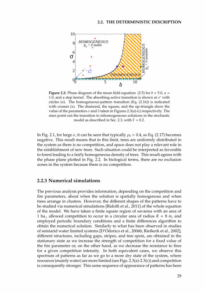
2.2. THE DETERMINISTIC DESCRIPTION
0 5 10δ0
2
4
6
8
10
σ
INHOMOGENEOUS
HOMOGENEOUS
HO
MO
GE
NE
OU
Sρ 0 =
0 u
nsta
ble
σ* =
ρ0 = 0 stable
1b-1
Figure 2.2: Phase diagram of the mean field equation (2.5) for b = 5.0, α =1.0, and a step kernel. The absorbing-active transition is shown at σ∗ withcircles (o). The homogeneous-pattern transition (Eq. (2.16)) is indicatedwith crosses (x). The diamond, the square, and the up-triangle show thevalue of the parameters σ and δ taken in Figures 2.3(a)-(c) respectively. Thestars point out the transition to inhomogeneous solutions in the stochastic
model as described in Sec. 2.3, with Γ = 0.2.
In Fig. 2.1, for large σ, it can be seen that typically ρ0 > 0.4, so Eq. (2.17) becomesnegative. This result means that in this limit, trees are uniformly distributed inthe system as there is no competition, and space does not play a relevant role inthe establishment of new trees. Such situation could be interpreted as favorableto forest leading to a fairly homogeneous density of trees. This result agrees withthe phase plane plotted in Fig. 2.2. In biological terms, there are no exclusionzones in the system because there is no competition.
2.2.3 Numerical simulations
The previous analysis provides information, depending on the competition andfire parameters, about when the solution is spatially homogenous and whentrees arrange in clusters. However, the different shapes of the patterns have tobe studied via numerical simulations [Ridolfi et al., 2011] of the whole equationof the model. We have taken a finite square region of savanna with an area of1 ha., allowed competition to occur in a circular area of radius R = 8 m, andemployed periodic boundary conditions and a finite differences algorithm toobtain the numerical solution. Similarly to what has been observed in studiesof semiarid water limited systems [D’Odorico et al., 2006b; Rietkerk et al., 2002],different structures, including gaps, stripes, and tree spots, are obtained in thestationary state as we increase the strength of competition for a fixed value ofthe fire parameter or, on the other hand, as we decrease the resistance to firesfor a given competition intensity. In both equivalent cases, we observe thisspectrum of patterns as far as we go to a more dry state of the system, whereresources (mainly water) are more limited (see Figs. 2.3(a)-2.3(c)) and competitionis consequently stronger. This same sequence of appearance of patterns has been
29
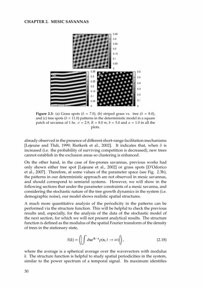
CHAPTER 2. MESIC SAVANNAS
Figure 2.3: (a) Grass spots (δ = 7.0), (b) striped grass vs. tree (δ = 8.0),and (c) tree spots (δ = 11.0) patterns in the deterministic model in a squarepatch of savanna of 1 ha. σ = 2.9, R = 8.0 m, b = 5.0 and α = 1.0 in all the
plots.
already observed in the presence of different short-range facilitation mechanisms[Lejeune and Tlidi, 1999; Rietkerk et al., 2002]. It indicates that, when δ isincreased (i.e. the probability of surviving competition is decreased), new treescannot establish in the exclusion areas so clustering is enhanced.
On the other hand, in the case of fire-prones savannas, previous works hadonly shown either tree spot [Lejeune et al., 2002] or grass spots [D’Odoricoet al., 2007]. Therefore, at some values of the parameter space (see Fig. 2.3b),the patterns in our deterministic approach are not observed in mesic savannas,and should correspond to semiarid systems. However, we will show in thefollowing sections that under the parameter constraints of a mesic savanna, andconsidering the stochastic nature of the tree growth dynamics in the system (i.e.demographic noise), our model shows realistic spatial structures.
A much more quantitative analysis of the periodicity in the patterns can beperformed via the structure function. This will be helpful to check the previousresults and, especially, for the analysis of the data of the stochastic model ofthe next section, for which we will not present analytical results. The structurefunction is defined as the modulus of the spatial Fourier transform of the densityof trees in the stationary state,
S(k) =⟨∣∣∣∣∣∫ dxeik · xρ(x, t→∞)
∣∣∣∣∣⟩ , (2.18)
where the average is a spherical average over the wavevectors with modulusk. The structure function is helpful to study spatial periodicities in the system,similar to the power spectrum of a temporal signal. Its maximum identifies
30
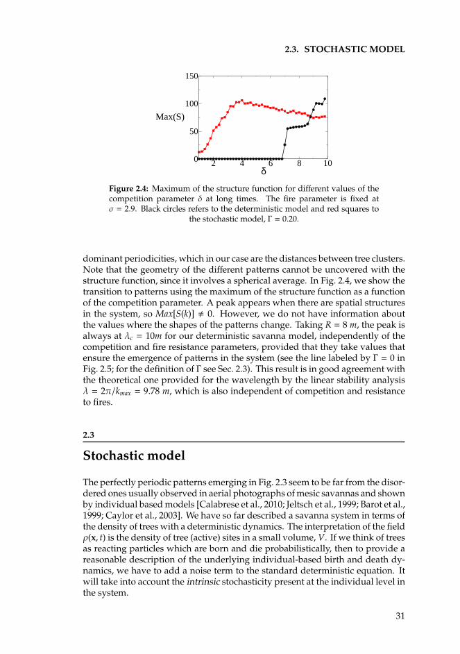
2.3. STOCHASTIC MODEL
2 4 6 8 10δ
0
50
100
150
Max(S)
Figure 2.4: Maximum of the structure function for different values of thecompetition parameter δ at long times. The fire parameter is fixed atσ = 2.9. Black circles refers to the deterministic model and red squares to
the stochastic model, Γ = 0.20.
dominant periodicities, which in our case are the distances between tree clusters.Note that the geometry of the different patterns cannot be uncovered with thestructure function, since it involves a spherical average. In Fig. 2.4, we show thetransition to patterns using the maximum of the structure function as a functionof the competition parameter. A peak appears when there are spatial structuresin the system, so Max[S(k)] , 0. However, we do not have information aboutthe values where the shapes of the patterns change. Taking R = 8 m, the peak isalways at λc = 10m for our deterministic savanna model, independently of thecompetition and fire resistance parameters, provided that they take values thatensure the emergence of patterns in the system (see the line labeled by Γ = 0 inFig. 2.5; for the definition of Γ see Sec. 2.3). This result is in good agreement withthe theoretical one provided for the wavelength by the linear stability analysisλ = 2π/kmax = 9.78 m, which is also independent of competition and resistanceto fires.
2.3
Stochastic model
The perfectly periodic patterns emerging in Fig. 2.3 seem to be far from the disor-dered ones usually observed in aerial photographs of mesic savannas and shownby individual based models [Calabrese et al., 2010; Jeltsch et al., 1999; Barot et al.,1999; Caylor et al., 2003]. We have so far described a savanna system in terms ofthe density of trees with a deterministic dynamics. The interpretation of the fieldρ(x, t) is the density of tree (active) sites in a small volume, V. If we think of treesas reacting particles which are born and die probabilistically, then to provide areasonable description of the underlying individual-based birth and death dy-namics, we have to add a noise term to the standard deterministic equation. Itwill take into account the intrinsic stochasticity present at the individual level inthe system.
31
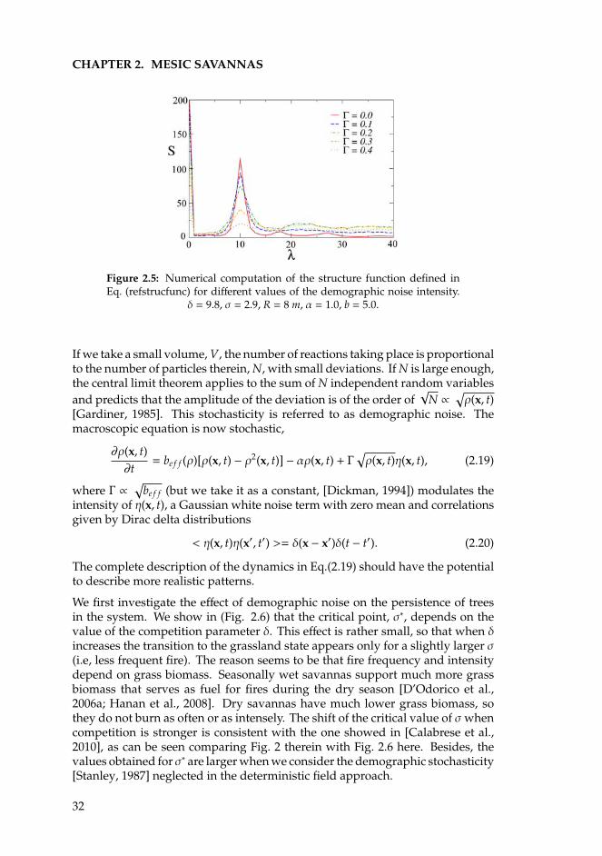
CHAPTER 2. MESIC SAVANNAS
Figure 2.5: Numerical computation of the structure function defined inEq. (refstrucfunc) for different values of the demographic noise intensity.
δ = 9.8, σ = 2.9, R = 8 m, α = 1.0, b = 5.0.
If we take a small volume, V, the number of reactions taking place is proportionalto the number of particles therein, N, with small deviations. If N is large enough,the central limit theorem applies to the sum of N independent random variablesand predicts that the amplitude of the deviation is of the order of
√N ∝
√ρ(x, t)
[Gardiner, 1985]. This stochasticity is referred to as demographic noise. Themacroscopic equation is now stochastic,
∂ρ(x, t)∂t
= be f f (ρ)[ρ(x, t) − ρ2(x, t)] − αρ(x, t) + Γ√ρ(x, t)η(x, t), (2.19)
where Γ ∝√
be f f (but we take it as a constant, [Dickman, 1994]) modulates theintensity of η(x, t), a Gaussian white noise term with zero mean and correlationsgiven by Dirac delta distributions
< η(x, t)η(x′, t′) >= δ(x − x′)δ(t − t′). (2.20)
The complete description of the dynamics in Eq.(2.19) should have the potentialto describe more realistic patterns.
We first investigate the effect of demographic noise on the persistence of treesin the system. We show in (Fig. 2.6) that the critical point, σ∗, depends on thevalue of the competition parameter δ. This effect is rather small, so that when δincreases the transition to the grassland state appears only for a slightly larger σ(i.e, less frequent fire). The reason seems to be that fire frequency and intensitydepend on grass biomass. Seasonally wet savannas support much more grassbiomass that serves as fuel for fires during the dry season [D’Odorico et al.,2006a; Hanan et al., 2008]. Dry savannas have much lower grass biomass, sothey do not burn as often or as intensely. The shift of the critical value of σwhencompetition is stronger is consistent with the one showed in [Calabrese et al.,2010], as can be seen comparing Fig. 2 therein with Fig. 2.6 here. Besides, thevalues obtained for σ∗ are larger when we consider the demographic stochasticity[Stanley, 1987] neglected in the deterministic field approach.
32
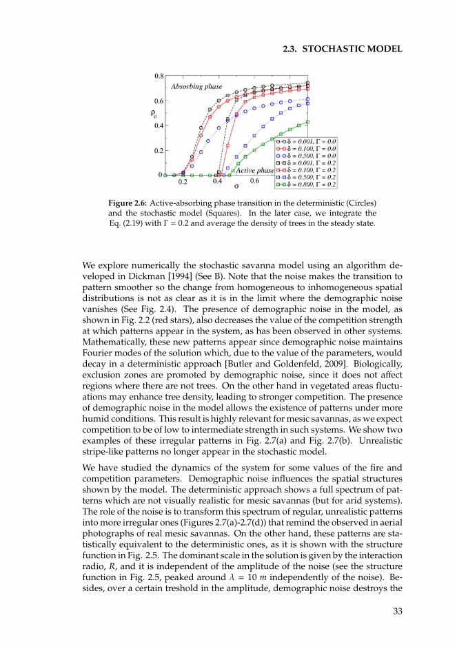
2.3. STOCHASTIC MODEL
Figure 2.6: Active-absorbing phase transition in the deterministic (Circles)and the stochastic model (Squares). In the later case, we integrate theEq. (2.19) with Γ = 0.2 and average the density of trees in the steady state.
We explore numerically the stochastic savanna model using an algorithm de-veloped in Dickman [1994] (See B). Note that the noise makes the transition topattern smoother so the change from homogeneous to inhomogeneous spatialdistributions is not as clear as it is in the limit where the demographic noisevanishes (See Fig. 2.4). The presence of demographic noise in the model, asshown in Fig. 2.2 (red stars), also decreases the value of the competition strengthat which patterns appear in the system, as has been observed in other systems.Mathematically, these new patterns appear since demographic noise maintainsFourier modes of the solution which, due to the value of the parameters, woulddecay in a deterministic approach [Butler and Goldenfeld, 2009]. Biologically,exclusion zones are promoted by demographic noise, since it does not affectregions where there are not trees. On the other hand in vegetated areas fluctu-ations may enhance tree density, leading to stronger competition. The presenceof demographic noise in the model allows the existence of patterns under morehumid conditions. This result is highly relevant for mesic savannas, as we expectcompetition to be of low to intermediate strength in such systems. We show twoexamples of these irregular patterns in Fig. 2.7(a) and Fig. 2.7(b). Unrealisticstripe-like patterns no longer appear in the stochastic model.
We have studied the dynamics of the system for some values of the fire andcompetition parameters. Demographic noise influences the spatial structuresshown by the model. The deterministic approach shows a full spectrum of pat-terns which are not visually realistic for mesic savannas (but for arid systems).The role of the noise is to transform this spectrum of regular, unrealistic patternsinto more irregular ones (Figures 2.7(a)-2.7(d)) that remind the observed in aerialphotographs of real mesic savannas. On the other hand, these patterns are sta-tistically equivalent to the deterministic ones, as it is shown with the structurefunction in Fig. 2.5. The dominant scale in the solution is given by the interactionradio, R, and it is independent of the amplitude of the noise (see the structurefunction in Fig. 2.5, peaked around λ = 10 m independently of the noise). Be-sides, over a certain treshold in the amplitude, demographic noise destroys the
33

CHAPTER 2. MESIC SAVANNAS
Figure 2.7: Patterns of the stochastic model in a square patch of savannaof 1 ha. σ = 2.9, R = 8.0 m, b = 5.0 and α = 1.0 in all the plots. (a) Γ = 0.2,
δ = 3.0. (b) Γ = 0.2, δ = 5.0. (c) Γ = 0.1, δ = 10.0. (b) Γ = 0.2, δ = 10.0.
population of trees. Therefore, the model presents an active-absorbing transitionwith the noise strength, Γ, being the control parameter.
2.4
Discussion
Understanding the mechanisms that produce spatial patterns in savanna treepopulations has long been an area of interest among savanna ecologists [Skarpe,1991; Jeltsch et al., 1999; Barot et al., 1999; Caylor et al., 2003; Scanlon et al., 2007].A key step in such an analysis is defining the most parsimonious combinationof mechanisms that will produce the pattern in question. In this paper thecombination of long-range competition for resources and the facilitation inducedby fire are considered the responsible of the spatial structures, in the line ofstudies of vegetation pattern formation in arid systems, where also a combinationof long-range inhibition and short-range facilitation is introduced [Klausmeier,1999; Lefever and Lejeune, 1997; Rietkerk et al., 2002; von Hardenberg et al., 2001].The main difference is that the facilitation provided by the protection effect ofadult trees against fires in our savanna model takes the short-range facilitationto its infinitesimally short limit (i.e, local limit). Under this assumption we havestudied the conditions under which our model could account for patterns. Wehave shown that nonlocal competition combined with local facilitation inducesthe full range of observed spatial patterns, provided the competition term entersnonlinearly in the equation for the density of trees, and that competition is strongenough.
34
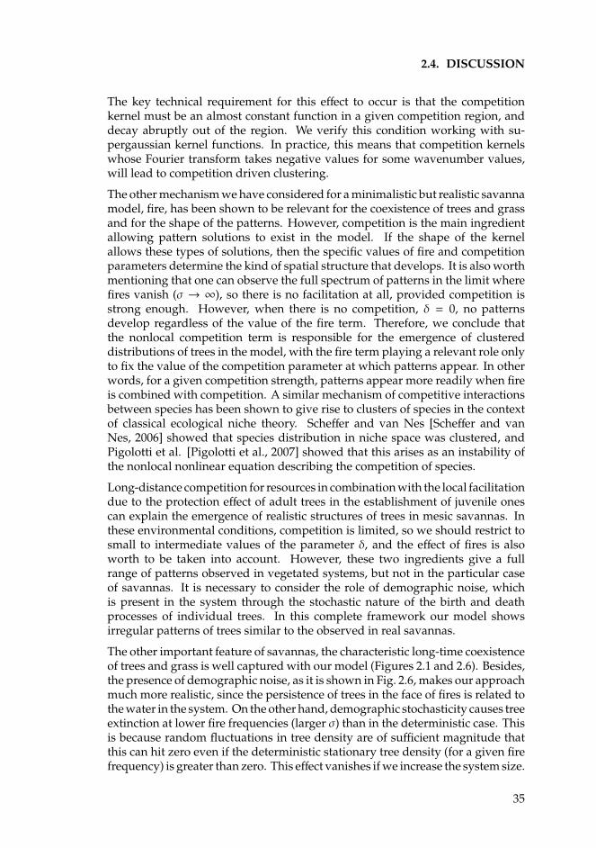
2.4. DISCUSSION
The key technical requirement for this effect to occur is that the competitionkernel must be an almost constant function in a given competition region, anddecay abruptly out of the region. We verify this condition working with su-pergaussian kernel functions. In practice, this means that competition kernelswhose Fourier transform takes negative values for some wavenumber values,will lead to competition driven clustering.
The other mechanism we have considered for a minimalistic but realistic savannamodel, fire, has been shown to be relevant for the coexistence of trees and grassand for the shape of the patterns. However, competition is the main ingredientallowing pattern solutions to exist in the model. If the shape of the kernelallows these types of solutions, then the specific values of fire and competitionparameters determine the kind of spatial structure that develops. It is also worthmentioning that one can observe the full spectrum of patterns in the limit wherefires vanish (σ → ∞), so there is no facilitation at all, provided competition isstrong enough. However, when there is no competition, δ = 0, no patternsdevelop regardless of the value of the fire term. Therefore, we conclude thatthe nonlocal competition term is responsible for the emergence of clustereddistributions of trees in the model, with the fire term playing a relevant role onlyto fix the value of the competition parameter at which patterns appear. In otherwords, for a given competition strength, patterns appear more readily when fireis combined with competition. A similar mechanism of competitive interactionsbetween species has been shown to give rise to clusters of species in the contextof classical ecological niche theory. Scheffer and van Nes [Scheffer and vanNes, 2006] showed that species distribution in niche space was clustered, andPigolotti et al. [Pigolotti et al., 2007] showed that this arises as an instability ofthe nonlocal nonlinear equation describing the competition of species.
Long-distance competition for resources in combination with the local facilitationdue to the protection effect of adult trees in the establishment of juvenile onescan explain the emergence of realistic structures of trees in mesic savannas. Inthese environmental conditions, competition is limited, so we should restrict tosmall to intermediate values of the parameter δ, and the effect of fires is alsoworth to be taken into account. However, these two ingredients give a fullrange of patterns observed in vegetated systems, but not in the particular caseof savannas. It is necessary to consider the role of demographic noise, whichis present in the system through the stochastic nature of the birth and deathprocesses of individual trees. In this complete framework our model showsirregular patterns of trees similar to the observed in real savannas.
The other important feature of savannas, the characteristic long-time coexistenceof trees and grass is well captured with our model (Figures 2.1 and 2.6). Besides,the presence of demographic noise, as it is shown in Fig. 2.6, makes our approachmuch more realistic, since the persistence of trees in the face of fires is related tothe water in the system. On the other hand, demographic stochasticity causes treeextinction at lower fire frequencies (larger σ) than in the deterministic case. Thisis because random fluctuations in tree density are of sufficient magnitude thatthis can hit zero even if the deterministic stationary tree density (for a given firefrequency) is greater than zero. This effect vanishes if we increase the system size.
35
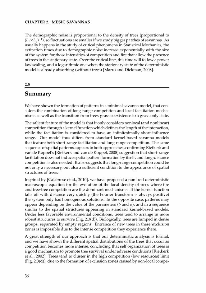
CHAPTER 2. MESIC SAVANNAS
The demographic noise is proportional to the density of trees (proportional to(Lx×Ly)−1), so fluctuations are smaller if we study bigger patches of savannas. Asusually happens in the study of critical phenomena in Statistical Mechanics, theextinction times due to demographic noise increase exponentially with the sizeof the system for those intensities of competition and fire that allow the presenceof trees in the stationary state. Over the critical line, this time will follow a powerlaw scaling, and a logarithmic one when the stationary state of the deterministicmodel is already absorbing (without trees) [Marro and Dickman, 2008].
2.5
Summary
We have shown the formation of patterns in a minimal savanna model, that con-siders the combination of long-range competition and local facilitation mecha-nisms as well as the transition from trees-grass coexistence to a grass only state.
The salient feature of the model is that it only considers nonlocal (and nonlinear)competition through a kernel function which defines the length of the interaction,while the facilitation is considered to have an infinitesimally short influencerange. Our model thus differs from standard kernel-based savanna modelsthat feature both short-range facilitation and long-range competition. The samesequence of spatial patterns appears in both approaches, confirming Rietkerk andvan de Koppel’s [Rietkerk and van de Koppel, 2008] suggestion that short-rangefacilitation does not induce spatial pattern formation by itself, and long-distancecompetition is also needed. It also suggests that long-range competition could benot only a necessary, but also a sufficient condition to the appearance of spatialstructures of trees.
Inspired by [Calabrese et al., 2010], we have proposed a nonlocal deterministicmacroscopic equation for the evolution of the local density of trees where fireand tree-tree competition are the dominant mechanisms. If the kernel functionfalls off with distance very quickly (the Fourier transform is always positive)the system only has homogenous solutions. In the opposite case, patterns mayappear depending on the value of the parameters (δ and σ), and in a sequencesimilar to the spatial structures appearing in standard kernel-based models.Under less favorable environmental conditions, trees tend to arrange in morerobust structures to survive (Fig. 2.3(d)). Biologically, trees are lumped in densegroups, separated by empty regions. Entrance of new trees in these exclusionzones is impossible due to the intense competition they experience there.
A great strength of our approach is that our deterministic analysis is formal,and we have shown the different spatial distributions of the trees that occur ascompetition becomes more intense, concluding that self organization of trees isa good mechanism to promote tree survival under adverse conditions [Rietkerket al., 2002]. Trees tend to cluster in the high competition (low resources) limit(Fig. 2.3(d)), due to the formation of exclusion zones caused by non-local compe-
36
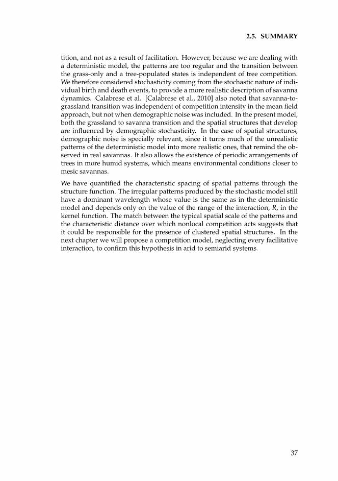
2.5. SUMMARY
tition, and not as a result of facilitation. However, because we are dealing witha deterministic model, the patterns are too regular and the transition betweenthe grass-only and a tree-populated states is independent of tree competition.We therefore considered stochasticity coming from the stochastic nature of indi-vidual birth and death events, to provide a more realistic description of savannadynamics. Calabrese et al. [Calabrese et al., 2010] also noted that savanna-to-grassland transition was independent of competition intensity in the mean fieldapproach, but not when demographic noise was included. In the present model,both the grassland to savanna transition and the spatial structures that developare influenced by demographic stochasticity. In the case of spatial structures,demographic noise is specially relevant, since it turns much of the unrealisticpatterns of the deterministic model into more realistic ones, that remind the ob-served in real savannas. It also allows the existence of periodic arrangements oftrees in more humid systems, which means environmental conditions closer tomesic savannas.
We have quantified the characteristic spacing of spatial patterns through thestructure function. The irregular patterns produced by the stochastic model stillhave a dominant wavelength whose value is the same as in the deterministicmodel and depends only on the value of the range of the interaction, R, in thekernel function. The match between the typical spatial scale of the patterns andthe characteristic distance over which nonlocal competition acts suggests thatit could be responsible for the presence of clustered spatial structures. In thenext chapter we will propose a competition model, neglecting every facilitativeinteraction, to confirm this hypothesis in arid to semiarid systems.
37

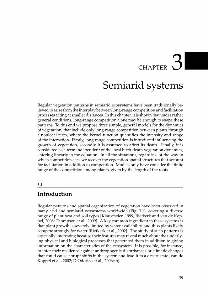
CHAPTER 3Semiarid systems
Regular vegetation patterns in semiarid ecosystems have been traditionally be-lieved to arise from the interplay between long-range competition and facilitationprocesses acting at smaller distances. In this chapter, it is shown that under rathergeneral conditions, long-range competition alone may be enough to shape thesepatterns. To this end we propose three simple, general models for the dynamicsof vegetation, that include only long-range competition between plants througha nonlocal term, where the kernel function quantifies the intensity and rangeof the interaction. Firstly, long-range competition is introduced influencing thegrowth of vegetation, secondly it is assumed to affect its death. Finally, it isconsidered as a term independent of the local birth-death vegetation dynamics,entering linearly in the equation. In all the situations, regardless of the way inwhich competition acts, we recover the vegetation spatial structures that accountfor facilitation in addition to competition. Models only have consider the finiterange of the competition among plants, given by the length of the roots.
3.1
Introduction
Regular patterns and spatial organization of vegetation have been observed inmany arid and semiarid ecosystems worldwide (Fig. 3.1), covering a diverserange of plant taxa and soil types [Klausmeier, 1999; Rietkerk and van de Kop-pel, 2008; Thompson et al., 2009]. A key common ingredient in these systems isthat plant growth is severely limited by water availability, and thus plants likelycompete strongly for water [Rietkerk et al., 2002]. The study of such patterns isespecially interesting because their features may reveal much about the underly-ing physical and biological processes that generated them in addition to givinginformation on the characteristics of the ecosystem. It is possible, for instance,to infer their resilience against anthropogenic disturbances or climatic changesthat could cause abrupt shifts in the system and lead it to a desert state [van deKoppel et al., 2002; D’Odorico et al., 2006c,b].
39
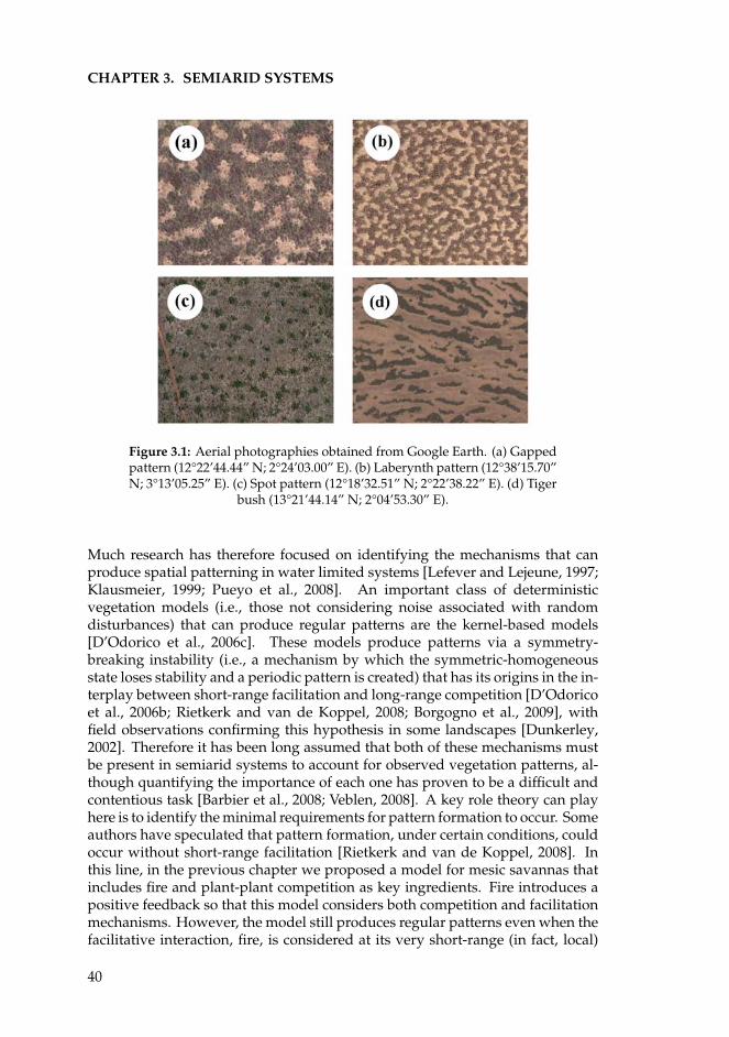
CHAPTER 3. SEMIARID SYSTEMS
Figure 3.1: Aerial photographies obtained from Google Earth. (a) Gappedpattern (12°22’44.44” N; 2°24’03.00” E). (b) Laberynth pattern (12°38’15.70”N; 3°13’05.25” E). (c) Spot pattern (12°18’32.51” N; 2°22’38.22” E). (d) Tiger
bush (13°21’44.14” N; 2°04’53.30” E).
Much research has therefore focused on identifying the mechanisms that canproduce spatial patterning in water limited systems [Lefever and Lejeune, 1997;Klausmeier, 1999; Pueyo et al., 2008]. An important class of deterministicvegetation models (i.e., those not considering noise associated with randomdisturbances) that can produce regular patterns are the kernel-based models[D’Odorico et al., 2006c]. These models produce patterns via a symmetry-breaking instability (i.e., a mechanism by which the symmetric-homogeneousstate loses stability and a periodic pattern is created) that has its origins in the in-terplay between short-range facilitation and long-range competition [D’Odoricoet al., 2006b; Rietkerk and van de Koppel, 2008; Borgogno et al., 2009], withfield observations confirming this hypothesis in some landscapes [Dunkerley,2002]. Therefore it has been long assumed that both of these mechanisms mustbe present in semiarid systems to account for observed vegetation patterns, al-though quantifying the importance of each one has proven to be a difficult andcontentious task [Barbier et al., 2008; Veblen, 2008]. A key role theory can playhere is to identify the minimal requirements for pattern formation to occur. Someauthors have speculated that pattern formation, under certain conditions, couldoccur without short-range facilitation [Rietkerk and van de Koppel, 2008]. Inthis line, in the previous chapter we proposed a model for mesic savannas thatincludes fire and plant-plant competition as key ingredients. Fire introduces apositive feedback so that this model considers both competition and facilitationmechanisms. However, the model still produces regular patterns even when thefacilitative interaction, fire, is considered at its very short-range (in fact, local)
40
3.2. COMPETITION IN A NONLOCAL NONLINEAR BIRTH TERM
limit. These considerations suggest that local facilitation may be superfluous forpattern formation, and that a deeper exploration of the range of conditions un-der which pattern formation can occur in the absence of facilitation is thereforewarranted. This will be the major concern of this chapter.
We will study simple, but quite general, single-variable models for vegetationdensity in water-limited regions. Only competitive interactions are considered,modeled in different ways to analyse if patterns depend on how competitionenters in the dynamical equations. The role of nonlinearities is also investigated.We show that when only a single broadly applicable condition is met, that com-petitive interactions have a finite range, the full set of regular patterns formerlyattributed to the interaction between short-range facilitation and long-distancecompetition can be produced in the absence of facilitation.
3.2
Competition in a nonlocal nonlinear birth term
Arid and semiarid ecosystems are typified by patches of vegetation interspersedwith bare ground. Water is a very limited resource for which juvenile plantsmust compete with those that have already established. Logistic-type popula-tion models have been used in a wide variety of applications including semi-arid systems and, as shown in the previous chapter, savannas [Calabrese et al.,2010]. They thus form a reasonable and very general starting point. Specifi-cally, we consider the large-scale long-time description of the model in termsof a continuous-time evolution equation for the density of trees, ρ(x, t). Deathoccurs at a constant rate α, whereas population growth occurs via a sequenceof seed production, dispersal, and seed establishment processes. Seed produc-tion occurs at a rate β0 per plant. For simplicity we consider dispersal to bepurely local and then if all seeds would give rise to new plants the growth ratewould be β0ρ(x, t). But once a seed lands, it will have to overcome competitionin order to establish as a new plant. We consider two different competitionmechanisms. First, space availability alone limits density to a maximum valuegiven by ρmax. Thus, 0 ≤ ρ(x, t) ≤ ρmax. The proportion of available space atsite x is 1 − ρ(x, t)/ρmax, so that the growth rate given by seed production shouldbe reduced by this factor. Second, once the seed germinates, it has to overcomecompetition for resources with other plants. This is included in the model by anadditional factor r = r(ρ, δ), 0 ≤ r ≤ 1, which is the probability of overcomingcompetition. This probability decreases with increasing average vegetation den-sity within a neighborhood ρ, and the strength of this decrease depends on thecompetition intensity parameter, δ. Higher values of δ represent more arid lands,and thus stronger competition for water. In the following, we measure densityin units so that ρmax = 1. Combining all processes, the evolution equation for thedensity then takes the form:
41
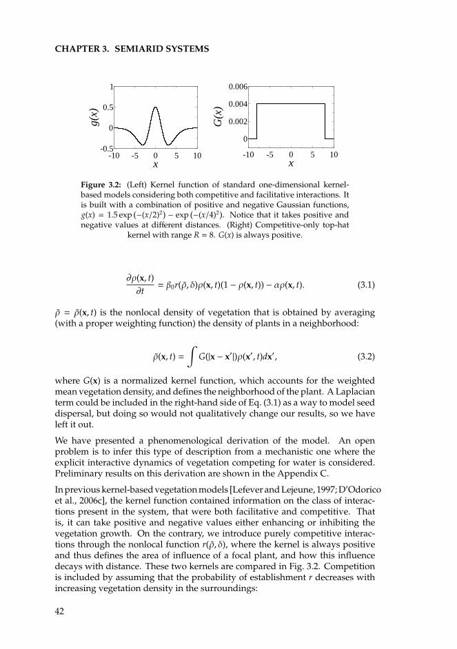
CHAPTER 3. SEMIARID SYSTEMS
-10 -5 0 5 10x
-0.5
0
0.5
1g(
x)
-10 -5 0 5 10x
0
0.002
0.004
0.006
G(x
)
Figure 3.2: (Left) Kernel function of standard one-dimensional kernel-based models considering both competitive and facilitative interactions. Itis built with a combination of positive and negative Gaussian functions,g(x) = 1.5 exp
(−(x/2)2) − exp(−(x/4)2). Notice that it takes positive and
negative values at different distances. (Right) Competitive-only top-hatkernel with range R = 8. G(x) is always positive.
∂ρ(x, t)∂t
= β0r(ρ, δ)ρ(x, t)(1 − ρ(x, t)) − αρ(x, t). (3.1)
ρ = ρ(x, t) is the nonlocal density of vegetation that is obtained by averaging(with a proper weighting function) the density of plants in a neighborhood:
ρ(x, t) =∫
G(|x − x′|)ρ(x′, t)dx′, (3.2)
where G(x) is a normalized kernel function, which accounts for the weightedmean vegetation density, and defines the neighborhood of the plant. A Laplacianterm could be included in the right-hand side of Eq. (3.1) as a way to model seeddispersal, but doing so would not qualitatively change our results, so we haveleft it out.
We have presented a phenomenological derivation of the model. An openproblem is to infer this type of description from a mechanistic one where theexplicit interactive dynamics of vegetation competing for water is considered.Preliminary results on this derivation are shown in the Appendix C.
In previous kernel-based vegetation models [Lefever and Lejeune, 1997; D’Odoricoet al., 2006c], the kernel function contained information on the class of interac-tions present in the system, that were both facilitative and competitive. Thatis, it can take positive and negative values either enhancing or inhibiting thevegetation growth. On the contrary, we introduce purely competitive interac-tions through the nonlocal function r(ρ, δ), where the kernel is always positiveand thus defines the area of influence of a focal plant, and how this influencedecays with distance. These two kernels are compared in Fig. 3.2. Competitionis included by assuming that the probability of establishment r decreases withincreasing vegetation density in the surroundings:
42
3.2. COMPETITION IN A NONLOCAL NONLINEAR BIRTH TERM
∂r(ρ, δ)∂ρ
≤ 0. (3.3)
As δmodulates the strength of the competition, it must be that r(ρ, δ = 0) = 1, andr(ρ, δ → ∞) = 0. This means that when water is abundant (δ = 0) competitionfor water is not important (r = 1), whereas new plants cannot establish in thelimit of extremely arid systems, δ→∞.
Note the generality of this vegetation competition model: a spatially nonlocalpopulation growth term of logistic type with rate fulfilling Eq. (3.3), and a lineardeath term. A complete description of our model should specify both the kernelfunction G as well as r, but we can go further with the analysis in general terms.
The possible homogenous stationary values of the density for Eq. (3.1) are: a) novegetation ρ = 0, and b) the vegetated state ρ = ρ0. The system will show eitherone or the other depending on the relationship between the seed productionand death rates, β0 and α [Calabrese et al., 2010]. The non-trivial homogeneousstationary solution, ρ0, can be obtained by solving
β0r(ρ0, δ)(1 − ρ0) − α = 0, (3.4)
that has only one solution in the interval ρ0 ∈ [0, 1] because of the conditionsimposed on the function r in equation(3.3). We now ask if this stationary solutiongives rise to periodic structures via a symmetry-breaking instability as happensin other models that include not only competition but also facilitation mecha-nisms in the interactions [Borgogno et al., 2009]. To explore this possibility in ourmodel, we perform a linear stability analysis [Cross and Hohenberg, 1993] intro-ducing a small perturbation to the stationary solution, so ρ(x, t) = ρ0 + εψ(x, t),with ε 1. Technical details of this derivation may be found in Appendix A.The perturbation growth rate is
λ(k) = −αρ0
[1
1 − ρ0−
r′(ρ0, δ)r(ρ0, δ)
G(k)], (3.5)
where G(k) is the Fourier transform of the kernel, G(k) =∫
G(x) exp(ik · x)dx,and r′(ρ0, δ) ≡
(∂r∂ρ
)ρ=ρ0
.
Patterns appear if the maximum of the growth rate (i.e., of the most unstablemode), λ(kc), is positive, which means that the perturbation grows with time.From Eq. (3.5), this is only possible if the Fourier transform of the kernel function,G(k), takes negative values, since r′(ρ0, δ) < 0. As has been in the previous chap-ter, this happens, for example, for all stretched exponentials G(|x|) ∝ exp (−|x/R|p)with p > 2, where R is a typical interaction length [Pigolotti et al., 2007, 2010].Kernels satisfying this criterion have broader shoulders and shorter tails (i.e.,are more platykurtic) than the Gaussian function, which is obtained for p = 2. Inreality, any competitive interaction among plants will have finite range becausetheir roots, which mediate the interaction, have finite length. The interactionrange R between two plants will be twice the typical root length. Kernels with
43
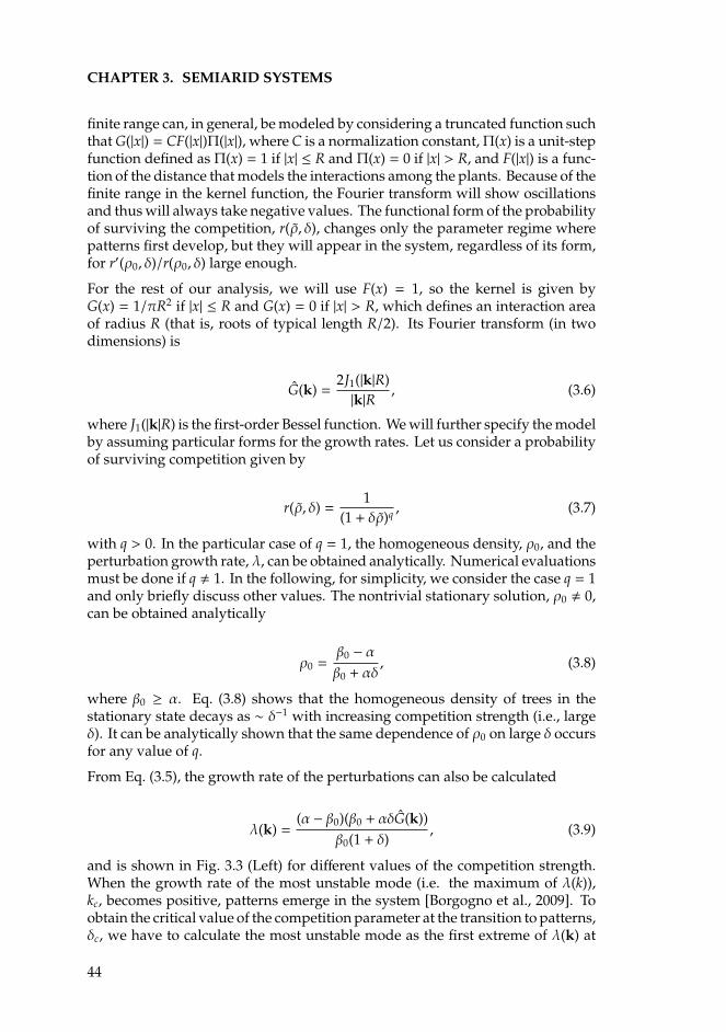
CHAPTER 3. SEMIARID SYSTEMS
finite range can, in general, be modeled by considering a truncated function suchthat G(|x|) = CF(|x|)Π(|x|), where C is a normalization constant,Π(x) is a unit-stepfunction defined as Π(x) = 1 if |x| ≤ R and Π(x) = 0 if |x| > R, and F(|x|) is a func-tion of the distance that models the interactions among the plants. Because of thefinite range in the kernel function, the Fourier transform will show oscillationsand thus will always take negative values. The functional form of the probabilityof surviving the competition, r(ρ, δ), changes only the parameter regime wherepatterns first develop, but they will appear in the system, regardless of its form,for r′(ρ0, δ)/r(ρ0, δ) large enough.
For the rest of our analysis, we will use F(x) = 1, so the kernel is given byG(x) = 1/πR2 if |x| ≤ R and G(x) = 0 if |x| > R, which defines an interaction areaof radius R (that is, roots of typical length R/2). Its Fourier transform (in twodimensions) is
G(k) =2J1(|k|R)|k|R , (3.6)
where J1(|k|R) is the first-order Bessel function. We will further specify the modelby assuming particular forms for the growth rates. Let us consider a probabilityof surviving competition given by
r(ρ, δ) =1
(1 + δρ)q , (3.7)
with q > 0. In the particular case of q = 1, the homogeneous density, ρ0, and theperturbation growth rate, λ, can be obtained analytically. Numerical evaluationsmust be done if q , 1. In the following, for simplicity, we consider the case q = 1and only briefly discuss other values. The nontrivial stationary solution, ρ0 , 0,can be obtained analytically
ρ0 =β0 − αβ0 + αδ
, (3.8)
where β0 ≥ α. Eq. (3.8) shows that the homogeneous density of trees in thestationary state decays as ∼ δ−1 with increasing competition strength (i.e., largeδ). It can be analytically shown that the same dependence of ρ0 on large δ occursfor any value of q.
From Eq. (3.5), the growth rate of the perturbations can also be calculated
λ(k) =(α − β0)(β0 + αδG(k))
β0(1 + δ), (3.9)
and is shown in Fig. 3.3 (Left) for different values of the competition strength.When the growth rate of the most unstable mode (i.e. the maximum of λ(k)),kc, becomes positive, patterns emerge in the system [Borgogno et al., 2009]. Toobtain the critical value of the competition parameter at the transition to patterns,δc, we have to calculate the most unstable mode as the first extreme of λ(k) at
44
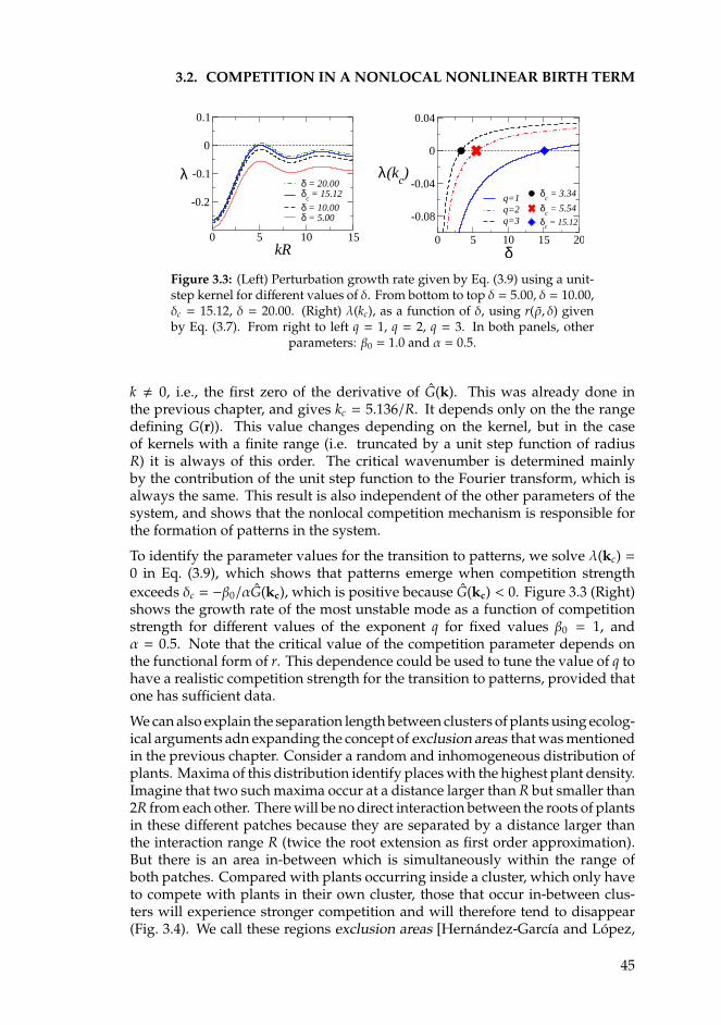
3.2. COMPETITION IN A NONLOCAL NONLINEAR BIRTH TERM
0 5 10 15kR
-0.2
-0.1
0
0.1
λδ = 20.00δ
c = 15.12
δ = 10.00δ = 5.00
0 5 10 15 20δ
-0.08
-0.04
0
0.04
λ(kc)
q=1q=2q=3
δc = 3.34
δc = 5.54
δc = 15.12
Figure 3.3: (Left) Perturbation growth rate given by Eq. (3.9) using a unit-step kernel for different values of δ. From bottom to top δ = 5.00, δ = 10.00,δc = 15.12, δ = 20.00. (Right) λ(kc), as a function of δ, using r(ρ, δ) givenby Eq. (3.7). From right to left q = 1, q = 2, q = 3. In both panels, other
parameters: β0 = 1.0 and α = 0.5.
k , 0, i.e., the first zero of the derivative of G(k). This was already done inthe previous chapter, and gives kc = 5.136/R. It depends only on the the rangedefining G(r)). This value changes depending on the kernel, but in the caseof kernels with a finite range (i.e. truncated by a unit step function of radiusR) it is always of this order. The critical wavenumber is determined mainlyby the contribution of the unit step function to the Fourier transform, which isalways the same. This result is also independent of the other parameters of thesystem, and shows that the nonlocal competition mechanism is responsible forthe formation of patterns in the system.
To identify the parameter values for the transition to patterns, we solve λ(kc) =0 in Eq. (3.9), which shows that patterns emerge when competition strengthexceeds δc = −β0/αG(kc), which is positive because G(kc) < 0. Figure 3.3 (Right)shows the growth rate of the most unstable mode as a function of competitionstrength for different values of the exponent q for fixed values β0 = 1, andα = 0.5. Note that the critical value of the competition parameter depends onthe functional form of r. This dependence could be used to tune the value of q tohave a realistic competition strength for the transition to patterns, provided thatone has sufficient data.
We can also explain the separation length between clusters of plants using ecolog-ical arguments adn expanding the concept of exclusion areas that was mentionedin the previous chapter. Consider a random and inhomogeneous distribution ofplants. Maxima of this distribution identify places with the highest plant density.Imagine that two such maxima occur at a distance larger than R but smaller than2R from each other. There will be no direct interaction between the roots of plantsin these different patches because they are separated by a distance larger thanthe interaction range R (twice the root extension as first order approximation).But there is an area in-between which is simultaneously within the range ofboth patches. Compared with plants occurring inside a cluster, which only haveto compete with plants in their own cluster, those that occur in-between clus-ters will experience stronger competition and will therefore tend to disappear(Fig. 3.4). We call these regions exclusion areas [Hernandez-Garcıa and Lopez,
45
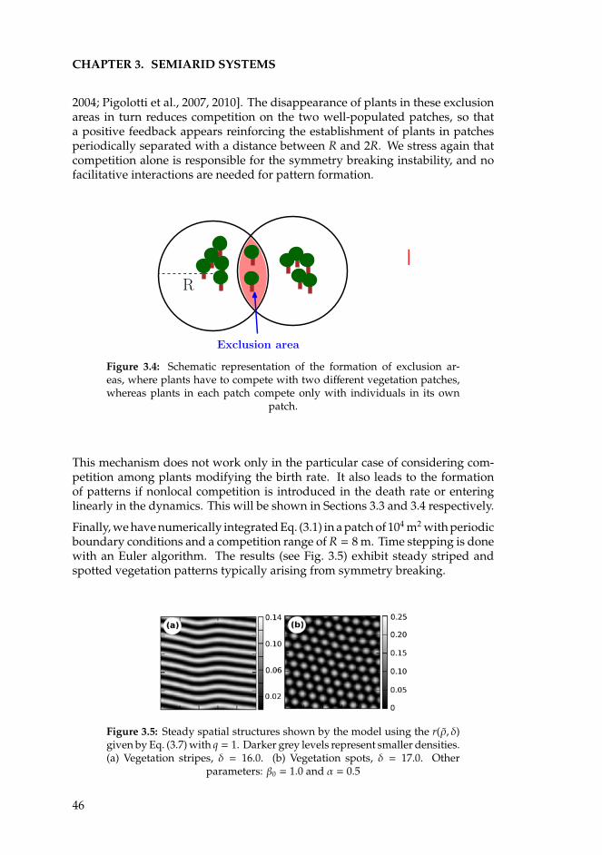
CHAPTER 3. SEMIARID SYSTEMS
2004; Pigolotti et al., 2007, 2010]. The disappearance of plants in these exclusionareas in turn reduces competition on the two well-populated patches, so thata positive feedback appears reinforcing the establishment of plants in patchesperiodically separated with a distance between R and 2R. We stress again thatcompetition alone is responsible for the symmetry breaking instability, and nofacilitative interactions are needed for pattern formation.
R
Exclusion area
Figure 3.4: Schematic representation of the formation of exclusion ar-eas, where plants have to compete with two different vegetation patches,whereas plants in each patch compete only with individuals in its own
patch.
This mechanism does not work only in the particular case of considering com-petition among plants modifying the birth rate. It also leads to the formationof patterns if nonlocal competition is introduced in the death rate or enteringlinearly in the dynamics. This will be shown in Sections 3.3 and 3.4 respectively.
Finally, we have numerically integrated Eq. (3.1) in a patch of 104 m2 with periodicboundary conditions and a competition range of R = 8 m. Time stepping is donewith an Euler algorithm. The results (see Fig. 3.5) exhibit steady striped andspotted vegetation patterns typically arising from symmetry breaking.
Figure 3.5: Steady spatial structures shown by the model using the r(ρ, δ)given by Eq. (3.7) with q = 1. Darker grey levels represent smaller densities.(a) Vegetation stripes, δ = 16.0. (b) Vegetation spots, δ = 17.0. Other
parameters: β0 = 1.0 and α = 0.5
46

3.3. COMPETITION IN A NONLOCAL NONLINEAR DEATH TERM
0 20 40 60δ
-0.4
-0.2
0
0.2
0.4
λ(kc)
s = 1 s = 2 s = 3
δc = 9.00
δc = 19.76
δc = 35.28
Figure 3.6: Perturbation growth rate of the most unstable mode as a func-tion of the competition strength for different values of the exponent s. s = 1full line, s = 2 dashed line, and s = 3 dotted-dashed line. Other parameters:
α = 1, β0 = 5, and R = 8.
Similar results can be obtained for different growth rates, for example con-sidering a family of stretched exponentials in the probability of overcominglong-range competition r(ρ, δ) = exp
(−δρs).This gives a perturbation growth rate of the form
λ(k) = −αρ0
(1
1 − ρ0+ δsρp−1
0 G(k)), (3.10)
where the stationary density, ρ0 has to be obtained numerically from Eq. (3.4).The value of the competition parameter at the transition to patterns δc also hasto be obtained numerically for a given set of values of s, α, and β0. This criticalvalue is shown in Fig. 3.6 using a top-hat kernel for different values of s. It isrepresented the value of the perturbation growth rate of the most unstable modeλ(kc) as a function of the competition strength δ.
This further confirms our result that competition is the only necessary ingredientfor the formation of vegetation patterns in the present framework, and thatthis does not depend on the functional form of the probability of survivingcompetition (growth rate) provided it verifies the requirements given by Eq. (3.3).
3.3
Competition in a nonlocal nonlinear death term
In the previous section we have considered that plant death occurs at a constantrate and the birth process takes place following a sequence of seed production,dispersal and establishment. The establishment of new seeds has been studiedas a process depending on the density of vegetation in a given neighborhood.However, it is possible to consider it affecting the death rate.
In this framework, the population growth has two stages, namely seed produc-tion at rate β0 and local seed dispersal. This means that once a seed is producedby a plant, it still has to compete for available space, limiting the density of
47
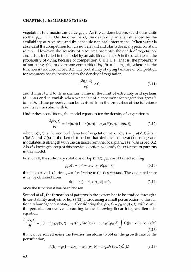
CHAPTER 3. SEMIARID SYSTEMS
vegetation to a maximum value ρmax. As it was done before, we choose unitsso that ρmax = 1. On the other hand, the death of plants is influenced by theavailability of resources and thus include nonlocal interactions. When water isabundant the competition for it is not relevant and plants die at a typical constantrate α0. However, the scarcity of resources promotes the death of vegetation,and this is included in the model by an additional factor h in the death term, theprobability of dying because of competition, 0 ≤ h ≤ 1. That is, the probabilityof not being able to overcome competition h(ρ, δ) = 1 − r(ρ, δ), where r is thefunction introduced in Sec. 3.2. The probability of dying because of competitionfor resources has to increase with the density of vegetation
∂h(ρ, δ)∂ρ
≥ 0, (3.11)
and it must tend to its maximum value in the limit of extremely arid systems(δ → ∞) and to vanish when water is not a constraint for vegetation growth(δ → 0). These properties can be derived from the properties of the function rand its relationship with h.
Under these conditions, the model equation for the density of vegetation is
∂ρ(x, t)∂t
= βρ(x, t)(1 − ρ(x, t)) − α0h(ρ(x, t), δ)ρ(x, t), (3.12)
where ρ(x, t) is the nonlocal density of vegetation at x, ρ(x, t) =∫ρ(x′, t)G(|x −
x′|)dx′, and G(x) is the kernel function that defines an interaction range andmodulates its strength with the distance from the focal plant, as it was in Sec. 3.2.Also following the step of this previous section, we study the existence of patternsin this model.
First of all, the stationary solutions of Eq. (3.12), ρ0, are obtained solving
βρ0(1 − ρ0) − α0h(ρ0, δ)ρ0 = 0, (3.13)
that has a trivial solution, ρ0 = 0 referring to the desert state. The vegetated statemust be obtained from
β(1 − ρ0) − α0h(ρ0, δ) = 0, (3.14)
once the function h has been chosen.
Second of all, the formation of patterns in the system has to be studied through alinear stability analysis of Eq. (3.12), introducing a small perturbation to the sta-tionary homogeneous state, ρ0. Considering thatρ(x, t) = ρ0+εψ(x, t), with ε 1,the perturbation evolves according to the following linear integro-differentialequation
∂ψ(x, t)∂t
= β(1− 2ρ0)ψ(x, t)−α0r(ρ0, δ)ψ(x, t)−α0ρ0r′(ρ0, δ)∫
G(|x−x′|)ψ(x′, t)dx′,
(3.15)that can be solved using the Fourier transform to obtain the growth rate of theperturbation,
λ(k) = β(1 − 2ρ0) − α0h(ρ0, δ) − α0ρ0h′(ρ0, δ)G(k), (3.16)
48
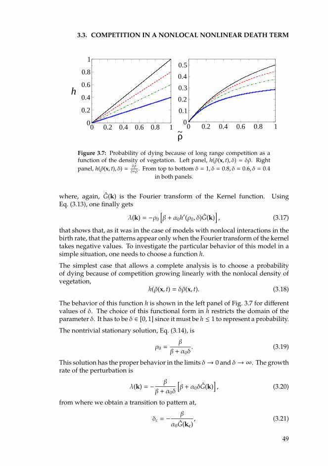
3.3. COMPETITION IN A NONLOCAL NONLINEAR DEATH TERM
0 0.2 0.4 0.6 0.8 10
0.2
0.4
0.6
0.8
1
h
0 0.2 0.4 0.6 0.8 10
0.1
0.2
0.3
0.4
0.5
ρ~
Figure 3.7: Probability of dying because of long range competition as afunction of the density of vegetation. Left panel, h(ρ(x, t), δ) = δρ. Rightpanel, h(ρ(x, t), δ) = δρ
δ+ρ . From top to bottom δ = 1, δ = 0.8, δ = 0.6, δ = 0.4in both panels.
where, again, G(k) is the Fourier transform of the Kernel function. UsingEq. (3.13), one finally gets
λ(k) = −ρ0
[β + α0h′(ρ0, δ)G(k)
], (3.17)
that shows that, as it was in the case of models with nonlocal interactions in thebirth rate, that the patterns appear only when the Fourier transform of the kerneltakes negative values. To investigate the particular behavior of this model in asimple situation, one needs to choose a function h.
The simplest case that allows a complete analysis is to choose a probabilityof dying because of competition growing linearly with the nonlocal density ofvegetation,
h(ρ(x, t) = δρ(x, t). (3.18)
The behavior of this function h is shown in the left panel of Fig. 3.7 for differentvalues of δ. The choice of this functional form in h restricts the domain of theparameter δ. It has to be δ ∈ [0, 1] since it must be h ≤ 1 to represent a probability.
The nontrivial stationary solution, Eq. (3.14), is
ρ0 =β
β + α0δ. (3.19)
This solution has the proper behavior in the limits δ→ 0 and δ→∞. The growthrate of the perturbation is
λ(k) = −β
β + α0δ
[β + α0δG(k)
], (3.20)
from where we obtain a transition to pattern at,
δc = −β
α0G(kc), (3.21)
49
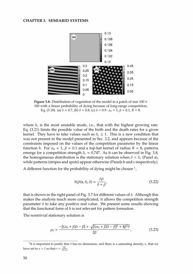
CHAPTER 3. SEMIARID SYSTEMS
Figure 3.8: Distribution of vegetation of the model in a patch of size 100 ×100 with a linear probability of dying because of long-range competition,
Eq. (3.18). (a) δ = 0.7, (b) δ = 0.8, (c) δ = 0.9. α0 = 1, β = 0.1, R = 8.
where kc is the most unstable mode, i.e., that with the highest growing rate.Eq. (3.21) limits the possible value of the birth and the death rates for a givenkernel. They have to take values such as δc ≤ 1. This is a new condition thatwas not present in the model presented in Sec. 3.2, and appears because of theconstraints imposed on the values of the competition parameter by the linearfunction h. For α0 = 1, β = 0.1 and a top-hat kernel of radius R = 8, patternsemerge for a competition strength δc ≈ 0.747. As it can be observed in Fig. 3.8,the homogeneous distribution is the stationary solution when δ < δc (Panel a),while patterns (stripes and spots) appear otherwise (Panels b and c respectively).
A different function for the probability of dying might be chosen 1,
h(ρ(x, t), δ) =δρ
δ + ρ, (3.22)
that is shown in the right panel of Fig. 3.7 for different values of δ. Although thismakes the analysis much more complicated, it allows the competition strengthparameter δ to take any positive real value. We present some results showingthat the functional form of h is not relevant for pattern formation.
The nontrivial stationary solution is
ρ0 =−[(α0 + β)δ − β] +
√[(α0 + β)δ − β]2 + 4β2δ
2β, (3.23)
1It is important to justify that δ has no dimension, and there is a saturating density, κ, that wehave set to κ = 1 so that r = δρ
δκ+ρ .
50
3.4. COMPETITION IN A NONLOCAL LINEAR DEATH TERM
where we have chosen the positive sign in the square root because it must beρ0 > 0. The growth rate of the perturbation is
λ(k) = −ρ0
[β +
α0δ2G(k)(δ + ρ0)2
]. (3.24)
Plugging Eq. (3.23) into Eq. (3.24) and considering the most unstable mode, kc,we can obtain an expression for the value of the competition parameter at thetransition to patterns,
δc =(α0 − β)G(kc) +
√α0β3(G(kc) − 1)2G(kc)
(α20 + β
2)G(kc) − α0β(G(kc) + 1)2. (3.25)
Using α0 = 1, β = 0.1 and a constant top-hat kernel of radius R = 8 one obtainsδc ≈ 0.663. This result can be checked integrating numerically Eq. (3.12) withthese values of the rates and the interaction range. We do not show this patternsagain because they are equivalent as the ones in Fig. 3.8.
3.4
Competition in a nonlocal linear death term
The study that we are going to present in this section is inspired by the kernel-based models reviewed in [Borgogno et al., 2009], where it is assumed that bothcompetitive and facilitative interactions between plants must come into playfor pattern formation. These models are not well posed, since the density ofvegetation can become negative at some spatial points because the long rangeinteractions entering linearly. This incovenience is often overcome assumingthat whenever the density becomes negative, it takes a value ρ(x, t) = 0. In thissection, we extend these models to the situations where there is only competitionamong trees, and also study the effect of seed dispersal through a diffusive term.The vegetation density changes in time because of its local dynamics (logisticgrowth) and the spatial interactions (competition) with other points of the space,
∂ρ(x, t)∂t
= D∇2ρ(x, t) + ρ(x, t)[1 − κ−1ρ(x, t)
]−Ω
∫G(|x − x′|)ρ(x′, t)dx′,
(3.26)
where κ is the carrying capacity of the system (i.e, the maximum density of vege-tation in the absence of competition) andΩ is the interaction strength parameter.To account for purely competitive interactionsΩ and the Kernel function G(x) arepositive. It is important to remark, once more, that the dynamics of this modelis not bounded at ρ(x, t) = 0, so negative values must be avoided by imposingthat ρ = 0 when it becomes negative in the numerical simulations.
The stationary solutions are, ρ0 = 0 (no vegetated state), and
ρ0 = (1 −Ω)κ, (3.27)
51
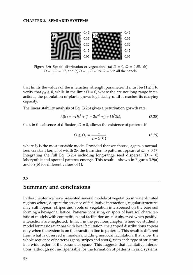
CHAPTER 3. SEMIARID SYSTEMS
Figure 3.9: Spatial distribution of vegetation. (a) D = 0, Ω = 0.85. (b)D = 1, Ω = 0.7, and (c) D = 1, Ω = 0.9. R = 8 in all the panels.
that limits the values of the interaction strength parameter. It must be Ω ≤ 1 toverify that ρ0 ≥ 0, while in the limit Ω = 0, where the are not long range inter-actions, the population of plants grows logistically until it reaches its carryingcapacity.
The linear stability analysis of Eq. (3.26) gives a peturbation gorwth rate,
λ(k) = −Dk2 + (1 − 2κ−1ρ0) +ΩG(k), (3.28)
that, in the absence of diffusion, D = 0, allows the existence of patterns if
Ω ≥ Ωc =1
2 − G(kc), (3.29)
where kc is the most unstable mode. Provided that we choose, again, a normal-ized constant kernel of width 2R the transition to patterns appears at Ωc ≈ 0.47.Integrating the full Eq. (3.26) including long-range seed dispersal (D , 0)laberynthic and spotted patterns emerge. This result is shown in Figures 3.9(a)and 3.9(b) for different values of Ω.
3.5
Summary and conclusions
In this chapter we have presented several models of vegetation in water-limitedregions where, despite the absence of facilitative interactions, regular structuresmay still appear: stripes and spots of vegetation interspersed on the bare soilforming a hexagonal lattice. Patterns consisting on spots of bare soil character-istic of models with competition and facilitation are not observed when positiveinteractions are neglected. In fact, in the previous chapter, where we studied amodel for mesic savannas with local facilitation, the gapped distributions appearonly when the system is on the transition line to patterns. This result is differentfrom what is observed in models including nonlocal facilitation, that show thewhole sequence of patterns (gaps, stripes and spots), with each type of structurein a wide region of the parameter space. This suggests that facilitative interac-tions, although not indispensable for the formation of patterns in arid systems,
52
3.5. SUMMARY AND CONCLUSIONS
could be relevant to substain some of the structures that have been reported infield observations. Future work is planned to address this problem.
From a mathematical point of view, nonlocality enters through an influencefunction that determines the number of plants competing within a range withany given plant. A first-order approximation of this distance can be given by(twice) the typical length of the roots, but field measurements are needed inorder to determine the resources uptaking range of a given plant species. Anecessary condition for pattern transitions, common to all the presented models,is the existence of negative values of the Fourier transform of the kernel function,which always happens, but not only, for kernel functions with finite range.
From a biological point of view, competitive interactions alone may give riseto spatial structures because of the development of regions (typically locatedbetween maxima of the plant density) where competition is stronger, preventingthe growth of more vegetation.
An unfortunate consequence of the universal character of these models is that theinformation that is possible to gain on the underlying biophysical mechanismsoperating in the system just by studying the spatial structures of the vegetationis limited. Many different mechanisms lead to the same patterns. Althoughthey are universal models should be specific to each system, emphasizing theimportance of empirical studies. Field work may help theoretical efforts byplacing biologically reasonable bounds on the shape and extent of the kernelfunctions used in the models, and also by approximations to the probablity ofovercoming competition, r(ρ, δ), or of dying because of it h(ρ, δ).
Finally, with this work, we aim at showing that competitive interactions alonemay be responsible of patterns in arid to semiarid systems, regardless of howthey are introduced in the different modeling approaches. Under certain condi-tions, nonlocal competition alone may be responsible of the formation of patternsregardless of entering in the equations either linearly or nonlinearly. We hopethat our results shed light on the task of understanding the fundamental biolog-ical mechanisms -and the possible absence of facilitation- that could be at theorigin of pattern formation in semiarid systems.
53

APPENDIX ALinear stability analysis
In chapters 2 and 3, we have referred many times to the linear stability analysisof the equations in order to gain insight into the possible emergence of patterns.This is a broadly used technique. Its objective is to obtain the temporal evolu-tion of small perturbations to the stationary homogeneous state of the system.To this aim we assume idealized conditions that can be summarized in threepoints: choosing a uniform geometry for the walls that confine the medium; re-placing the lateral boundaries with ones consistent with translational symmetry;and choosing to study the linear instability towards time-independent patternsthat are consistent with translational symmetry. We impose periodic boundaryconditions and study the formation of stationary patterns.
Our starting point is Eq. (3.1),
∂ρ(x, t)∂t
= β0r(ρ, δ)ρ(x, t)(1 − ρ(x, t)) − αρ(x, t). (A.1)
Considering that the system is in the homogeneous stationary state, ρ(x, t) =ρ0, how will perturbations to this state evolve with time? Will they vanish,taking the system back to the homogeneous state, or will they grow up allowingthe formation of stationary spatial structures? The key quantity will be thegrowth rate of the perturbation, restricted to the linear regime, so that only smallperturbations in the short time limit will be considered. If a small perturbationis done to the stationary homogeneous state, the density is
ρ(x, t) = ρ0 + εψ(x, t), (A.2)
with ε 1. Plugging Eq. (A.2) into Eq. (A.1), it is
ε∂ψ
∂t= β0r
(ρ0 + ε
∫ψ(x′, t)G(|x − x′|)dx′, δ
)(ρ0 + εψ)(1 − ρ0 − εψ) − α(ρ0 + εψ),
(A.3)where the spatiotemporal dependence in the perturbation ψ is omitted to sim-plify the notation. We have also used that ρ0 is stationary and thus its timederivative equals to zero together with the normalization of the kernel to sim-plify the dependence on ρ0 in the function r.
55
APPENDIX A. LINEAR STABILITY ANALYSIS
Eq. (A.3) can be simplified because we are interested in small perturbations.The function r can be expanded in a Taylor series and higher order terms in εneglected. This gives a linearized integro-differential equation for the evolutionof ψ,
∂ψ
∂t= β0r(ρ0, δ)(1 − 2ρ0)ψ − αρ0ψ + β0r′(ρ0, δ)ρ0(1 − ρ0)
∫G(|x − x′|)ψ(x′, t)dx′,
(A.4)
that can be solved using Fourier transform. Notice that the stationary solutionof Eq. (A.1),
β0r(ρ0, δ)ρ0(1 − ρ0) − αρ0 = 0, (A.5)
has been used to obtain Eq. (A.4). We apply the Fourier transform to Eq. (A.4),
∂ψ(k, t)∂t
= β0r(ρ0, δ)(1 − 2ρ0)ψ(k, t) − αρ0ψ(k, t)
+ β0r′(ρ0, δ)ρ0(1 − ρ0)G(k)ψ(k, t), (A.6)
where ψ(k, t) =∫
eik · xψ(x, t)dx is the Fourier transform of the perturbation, andequivalently, G(k) is the Fourier transform of the kernel.
Finally, Eq. (A.6) is solved considering ψ(k, t) ∝ exp(λ(k)t), so that a lineargrowth rate of the perturbation is obtained
λ(k) = β0
[r(ρ0, δ)(1 − 2ρ0) + (1 − ρ0)ρ0r′(ρ0, δ)G(k)
]− α. (A.7)
56
APPENDIX BNumerical integration of
Eq. (2.19)
The integration of stochastic equations where the noise amplitude depends onthe square root of the variable, ρ, and there are absorbing states (i.e, states wherethe system stays indefinitely), has awaken a great interest, specially in the studyof critical phenomena (i.e, properties of the system that appear when it is close tothe critical point). The amplitude of the fluctuations tends to zero there, and thusnumerical instabilities may appear. Recently [Dornic et al., 2005; Pechenik andLevine, 1999] a very efficient method has been developed, but we have used inthis work an older one, presented in [Dickman, 1994], since its implementation iseasier and it gives precise results working far from the transition point. It consistson discretizing the Langevin equation, taking a step size ∆ρ in the variable.
First of all, to integrate the Eq. (2.19) we discretize the space, whose area is Lx×Ly,in a Nx ×Ny regular grid and compute the integral in the exponential term. It isapproximated by a sum of the field evaluated in the nodes∫
ρ(x, t)G(x − x′)dx ≈Nx∑i=1
Ny∑j=1
ρi, jGi, j;i′, j′∆x∆y, (B.1)
where ∆x and ∆y are the spatial steps in both directions. They are given by∆x,y = Lx,y/(Nx,y − 1).
Then, we integrate the temporal dependence. The key of the algorithm is toprevent ρ + ∆ρ to take negative values. From a general equation
dρdt= f (ρ) +
√ρη(t), (B.2)
where η(t) is a Gaussian white noise with zero mean and delta correlated, it is
∆ρ = f (ρ)∆t +√ρ∆W, (B.3)
where ∆W =√∆tY. Y is a Gaussian number with zero mean and unit variance.
To avoid negative values of ρ + ∆ρ, Dickman [1994] proposes to dicretize the
57
APPENDIX B. NUMERICAL INTEGRATION OF EQ. (2.19)
density setting ρ = nρmin and to simetrically truncate the Gaussian distributionfrom where Y is drawn, so that |Y| ≤ Ymax. The negative values are avoidedrequiring
Ymax√∆t ≤ ρmin. (B.4)
This can be seen adding ρ in both sides of Eq. (B.3), considering the discretizationof the density and assuming that Y takes its most negative value according tothe constraint (B.4), so
nρmin + ∆ρ = f (nρmin)∆t + nρmin −√
nρmin, (B.5)
that is always positive for n integer.
Eq. (B.4) can be verified in many ways but, following Dickman [1994] again, weuse
Ymax =| ln∆t|
3,
ρmin =(ln∆t)2∆t
9. (B.6)
Finally, rescaling the equation, we can achieve a discretized version in whichpositive and zero-mean noise are ensured at the cost of a “quantized” density.
58
APPENDIX CDerivation of the effectivenonlocal description from
tree-water dynamics
In this section we present a preliminar (and not fully satisfactory) attempt toderive the model presented in Section 3.2 of Chapter 3 (the derivation corre-sponding to the nonlocal death model in 3.3 is a straightforward extension ofthis calculation).
Let us consider a system involving dimensionless vegetation density, ρ(x, t), andsoil-water w(x, t). The dynamics is purely local and competitive and takes theform:
∂ρ
∂t= βρ(1 − ρ)w − αρ, (C.1)
∂w∂t
= −µρw − γw + I +Dw∇2w, (C.2)
where the nondimensional positive parameters are: the seed production rateβ; the vegetation death rate α; the consumption rate of water by vegetation, µ;the evaporation rate γ, and the rainfall, I. Water percolation in the ground ismodeled by a diffusion constant Dw. Note that this model is a simplified version,which only includes competitive interactions, of the model presented in Giladet al. [2004].
Since the characteristic time scale of the water is much faster than the one of thebiomass we can do an adiabatic elimination of the variable w (i.e. ∂w
∂t = 0) so that
− µρw − γw + I +Dw∇2w = 0, (C.3)
and thus (Dw∇2 − γ
)w = µρw − I, (C.4)
whose formal solution can be obtained using Green’s functions, Gd,
w(x) =∫
Gd(x − s)(µρ(s)w(s) − I)ds, (C.5)
59
APPENDIX C. DERIVATION OF THE EFFECTIVE NONLOCALDESCRIPTION FROM TREE-WATER DYNAMICS
with the boundary conditions w(x→ ±∞) = 0. For simplicity we now consider aone-dimensional situation, although analogous calculations can be done in twodimensions. The Green’s function is the solution of(
Dw∇2 − γ)
Gd = δ(x − s), (C.6)
and it is given by
Gd(x, s) = −12
exp(−
√γ
Dw|x − s|
)(C.7)
Taking the nondimensional small number µ as the perturbative parameter, wecan further obtain an approximate expression for w from Eq. (C.5)
w(x) = −IGd0
[1 + µ
∫Gd(x − s)ρ(s)ds + O(µ2)
], (C.8)
where Gd0 =∫
Gd(x − s)ds < 0, since the Green’s function is always negative.Plugging this in the equation for the biomass density (C.1), we obtain the closedexpression:
∂ρ
∂t= βρ(1 − ρ)
−IGd0
[µ
∫Gd(x − s)ρ(s)ds + 1
]− αρ. (C.9)
Defining the positive nonlocal density ρ =∫
Gc(x− s)ρ(s)ds, where Gc = −Gd, wecan write Eq. (C.9) as
∂ρ
∂t= βr(ρ)ρ(1 − ρ) − αρ, (C.10)
where we have defined r(ρ) = I|Gd0|(1 − µρ).
To have a good agreement with the effective nonlocal dynamics Eq. (3.1), r > 0since it represents a probability. This is certainly the case for small µ. Note thatsome additional conditions on the normalization of the Green’s function haveto be imposed to limit r to values less than 1. Also r′(ρ) = −Iµ|Gd0| is alwaysnegative, as we expected.
In this particular example we obtained the exponential kernel of Eq. (C.7), whichdoes not have the finite-range support that would be associated to the finite rootextent. As a consequence, the Fourier transform of this kernel has no negativecomponents and then does not lead to pattern formation. The simple modeling ofwater dispersion by means of a diffusion constant does not contain the additionalspatial scale associated to root size, and should be replaced by some mechanismimplementing root effects. On the other side, the finite-range of the kernel is asufficient but not a necessary condition for its Fourier transform to have negativevalues. It is well-known the existence of infinite-range kernels whose Fouriertransform has negative values. This is the case of all stretched exponentialsG(x) ∝ exp(−|x|p) with p > 2 as has been already mentioned several times before.Kernels satisfying this are more platykurtic than the Gaussian function. Work isin progress along this line.
60
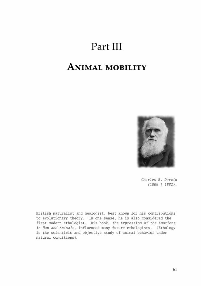
Part III
Animal mobility
Charles R. Darwin
(1809 1882).
British naturalist and geologist, best known for his contributions
to evolutionary theory. In one sense, he is also considered the
first modern ethologist. His book, The Expression of the Emotions
in Man and Animals, influenced many future ethologists. (Ethology
is the scientific and objective study of animal behavior under
natural conditions).
61

CHAPTER 4Optimal search in interacting
populations
In this chapter we investigate the relationships between search efficiency, move-ment strategy, and non-local communication in the biological context of animalforaging. We consider situations where the members of a population of foragersperform either Gaussian jumps or Levy flights, and show that the search timeis minimized when communication among individuals occurs at intermediateranges, independently of the type of movement. While Brownian strategies aremore strongly influenced by the communication mechanism, Levy flights stillresult in shorter overall search durations.
4.1
Introduction
Situations where a single individual or a group of searchers must find anobject (target) appear in many different fields including chemistry [Benichouet al., 2011], information theory [Pirolli and Card, 1999], and animal foraging[Viswanathan et al., 2011; Mendez et al., 2014]. The study of these searchingproblems has generated an increasing amount of work in the last years, many ofthem oriented towards the identification of efficient strategies [Benichou et al.,2011; Viswanathan et al., 2011; Vergassola et al., 2007; Benichou et al., 2006].Many remarkable examples can be found in the context of biological encounters,such as proteins searching for targets on DNA [Taylor and Halford, 1989], or an-imals searching for a mate, shelter or food [Campos et al., 2013; Benichou et al.,2011; Viswanathan et al., 1999; Shlesinger, 2006; Edwards et al., 2007; Torney et al.,2011; Hein and McKinley, 2012; Viswanathan et al., 2008; Mejıa-Monasterio et al.,2011; Bartumeus et al., 2003]. In these cases, the search time is generally limitingand minimizing it can increase individual fitness or reaction rates.
The optimality of a search strategy depends strongly on the nature of both thetargets and the searchers [Bartumeus et al., 2005, 2002]. In the context of animal
63
CHAPTER 4. OPTIMAL SEARCH IN INTERACTING POPULATIONS
foraging, which is our focus here, searchers may move randomly, may usememory and experience to locate dispersed targets or they may also combinerandom search with memory-based search. In highly social species, groupsof searchers may share information when no single individual is sufficientlyknowledgeable. This is based on the many wrong hypothesis [Hoare et al.,2004; Torney et al., 2009a], that states that error in sensing of individuals can bereduced by interacting with the rest of the group, where all individuals can actas sensors.
It is well known that individual movement plays a central role in search effi-ciency, and many studies have focused on the comparative efficiency of Levyand Brownian movement strategies [Benichou et al., 2011; Viswanathan et al.,2008; Bartumeus et al., 2005, 2002]. Levy flights are more efficient in some ran-dom search scenarios [Viswanathan et al., 1999, 2000], but whether or not theyare used in real animal search strategies is still an open and contentious topic[Edwards, 2011; Edwards et al., 2007]. Much less effort, however, has been spenton trying to understand the long-range (i.e. nonlocal) interaction mechanismsamong social searchers. While diverse observations suggest that such interac-tions occur in many taxa, including bacteria [Liu and Passino, 2002], insects, andmammals [Zuberbuhler et al., 1997; McComb et al., 2003], previous studies havefocused almost exclusively on how the collective movements of a group of ani-mals can emerge from local interactions among individuals [Mishra et al., 2012;Kolpas et al., 2013; Couzin et al., 2002]. The distance at which communicationcan be maintained strongly depends on the species. A variety of mammalianspecies are known to communicate acoustically over distances of up to severalkilometers [McComb et al., 2003; Mathevon et al., 2010; Estes, 1991], but whilegroup formation via vocalizations has been well studied [McComb et al., 2003;Ford, 1991; Smith et al., 2011], incidental benefits such as increased foraging ef-ficiency have received little research attention. Therefore many open questionsremain, particularly on the interrelation between communication and optimalsearch for resources. How can communication facilitate group formation andidentification of areas of high quality resources? Does a communication rangeexist that optimizes foraging efficiency? To what degree does search efficiencydepend on the communication mechanism? Finally, how does communicationaffect individual space use in a heterogeneous environment?
Here, we present a theoretical model to study the effect of nonlocal communica-tion on the search efficiency of a group of individuals. Communication and theamount of shared information are directly connected through the distance trav-elled by the signals emitted by successful searchers (communication range). Tointroduce the model, we start from an individual based description and comparethe situations where the individuals employ either Levy or Brownian randomsearch strategies. In the first section we study many properties of the model suchas the existence of an optimal communication range and the influence of the dis-tance between targets and the movement strategy on its value. For tractability,we will next consider a simplified, one-dimensional version of the model andcompute analytically the search time for both Brownian and Levy searchers as afunction of the communication length scale. This simplified model allows us to
64
4.2. THE INDIVIDUAL BASED MODEL FOR BROWNIAN SEARCHERS
unveil the dependence of this time on both the parameters governing individualmobility, and on the distance between targets. Finally, a continuum descriptionin terms of an equation for the density of searchers is derived. The chapter endswith a discussion comparing Brownian and Levy strategies.
4.2
The Individual Based Model for Brownian searchers
We consider N particles which undergo a 2D Brownian random walk. Corre-lated random walks, often more appropriate to model directional persistence inanimal movement, reduce to Brownian motion for large spatiotemporal scales[Turchin, 1998]. The movement is biased by the gradients of the landscape quality(local information), and by the interaction among individuals through a com-munication mechanism that is activated when good resources are found, thusproviding information on habitat quality in other areas (nonlocal information).The dynamics of any of the particles i = 1, ...,N is
ri(t) = Bg∇g(ri) + BC∇S(ri) + ηi(t), (4.1)
where ηi(t) is a Gaussian white noise term characterized by 〈ηi(t)〉 = 0, and〈ηi(t)η j(t′)〉 = 2Dδi jδ(t − t′), with D the diffusion coefficient. The term Bg∇g(ri)refers to the local search, where g(r) is the environmental quality function(amount of grass, prey, etc...) and Bg is the local search bias parameter. BC∇S(ri)is the nonlocal search term, with BC the nonlocal search bias parameter andS(ri) is the available information function of the individual i. It represents theinformation arriving at the spatial position of the animal i as a result of the com-munication with the rest of the population. This term makes the individualsmove along the gradients of the information received. It is a function of thesuperposition of pairwise interactions between the individual i and each one ofits conspecifics,
S(ri) = F
N∑j=1, j,i
A[g(r j)]V(ri, r j)
. (4.2)
F is an arbitrary perception function that must be set in each application of themodel, V(ri, r j) is the interaction between the receptor particle i depending onits position ri and the emitting particle fixed at r j, and A[g(r j)] is the activationfunction (typically, a Heaviside function) that indicates that the individual at r jcalls the others if it is in a good habitat.
We begin with Monte Carlo simulations of the individual based dynamics inEq. (4.1) using a square system (Lx = Ly = 1) with periodic boundary conditions,and a population of N = 100 individuals. We use a theoretical landscape qualityfunction, g(r), consisting of three non-normalized Gaussian functions, to ensurethat g(r) ∈ [0, 1], centered at different spatial points (Fig. 4.1). As a first approach,we consider a Gaussian-like interaction kernel. Manipulating its typical rangevia the standard deviation, σ, the information sent by a successful searcher will
65
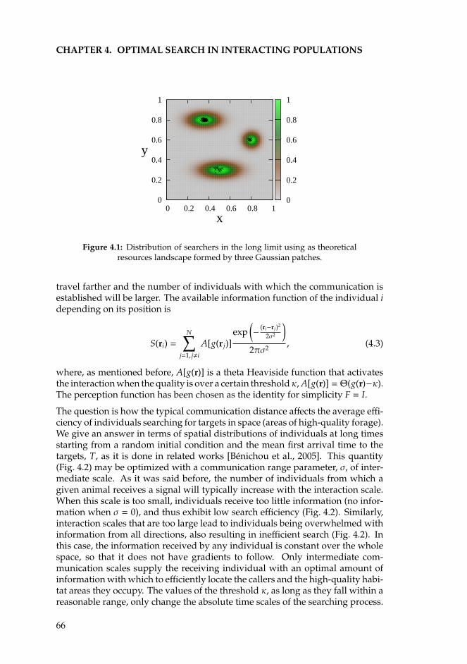
CHAPTER 4. OPTIMAL SEARCH IN INTERACTING POPULATIONS
0 0.2 0.4 0.6 0.8 1x
0
0.2
0.4
0.6
0.8
1
y
0
0.2
0.4
0.6
0.8
1
Figure 4.1: Distribution of searchers in the long limit using as theoreticalresources landscape formed by three Gaussian patches.
travel farther and the number of individuals with which the communication isestablished will be larger. The available information function of the individual idepending on its position is
S(ri) =N∑
j=1, j,i
A[g(r j)]exp
(− (ri−r j)2
2σ2
)2πσ2 , (4.3)
where, as mentioned before, A[g(r)] is a theta Heaviside function that activatesthe interaction when the quality is over a certain thresholdκ, A[g(r)] = Θ(g(r)−κ).The perception function has been chosen as the identity for simplicity F = I.
The question is how the typical communication distance affects the average effi-ciency of individuals searching for targets in space (areas of high-quality forage).We give an answer in terms of spatial distributions of individuals at long timesstarting from a random initial condition and the mean first arrival time to thetargets, T, as it is done in related works [Benichou et al., 2005]. This quantity(Fig. 4.2) may be optimized with a communication range parameter, σ, of inter-mediate scale. As it was said before, the number of individuals from which agiven animal receives a signal will typically increase with the interaction scale.When this scale is too small, individuals receive too little information (no infor-mation when σ = 0), and thus exhibit low search efficiency (Fig. 4.2). Similarly,interaction scales that are too large lead to individuals being overwhelmed withinformation from all directions, also resulting in inefficient search (Fig. 4.2). Inthis case, the information received by any individual is constant over the wholespace, so that it does not have gradients to follow. Only intermediate com-munication scales supply the receiving individual with an optimal amount ofinformation with which to efficiently locate the callers and the high-quality habi-tat areas they occupy. The values of the threshold κ, as long as they fall within areasonable range, only change the absolute time scales of the searching process.
66
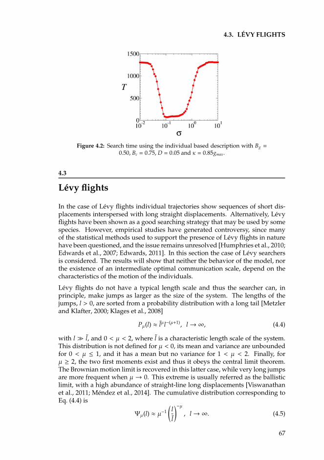
4.3. LEVY FLIGHTS
Figure 4.2: Search time using the individual based description with Bg =0.50, Bc = 0.75, D = 0.05 and κ = 0.85gmax.
4.3
Levy flights
In the case of Levy flights individual trajectories show sequences of short dis-placements interspersed with long straight displacements. Alternatively, Levyflights have been shown as a good searching strategy that may be used by somespecies. However, empirical studies have generated controversy, since manyof the statistical methods used to support the presence of Levy flights in naturehave been questioned, and the issue remains unresolved [Humphries et al., 2010;Edwards et al., 2007; Edwards, 2011]. In this section the case of Levy searchersis considered. The results will show that neither the behavior of the model, northe existence of an intermediate optimal communication scale, depend on thecharacteristics of the motion of the individuals.
Levy flights do not have a typical length scale and thus the searcher can, inprinciple, make jumps as larger as the size of the system. The lengths of thejumps, l > 0, are sorted from a probability distribution with a long tail [Metzlerand Klafter, 2000; Klages et al., 2008]
Pµ(l) ≈ lµl−(µ+1), l→∞, (4.4)
with l l, and 0 < µ < 2, where l is a characteristic length scale of the system.This distribution is not defined for µ < 0, its mean and variance are unboundedfor 0 < µ ≤ 1, and it has a mean but no variance for 1 < µ < 2. Finally, forµ ≥ 2, the two first moments exist and thus it obeys the central limit theorem.The Brownian motion limit is recovered in this latter case, while very long jumpsare more frequent when µ → 0. This extreme is usually referred as the ballisticlimit, with a high abundance of straight-line long displacements [Viswanathanet al., 2011; Mendez et al., 2014]. The cumulative distribution corresponding toEq. (4.4) is
Ψµ(l) ≈ µ−1
(ll
)−µ, l→∞. (4.5)
67
CHAPTER 4. OPTIMAL SEARCH IN INTERACTING POPULATIONS
As a simple normalizable cumulative distribution function, with the asymptoticbehavior of Eq. (4.5), we will use [Heinsalu et al., 2010]
Ψµ(l) =1
l(1 + l
lb1/µ
)µ , (4.6)
whose probability distribution, Pµ(l) = Ψ′µ(l), is given by
Pµ(l) =µb1/µ
l(1 + l
lb1/µ
)µ+1 , (4.7)
with 0 < µ < 2, and b = [Γ(1 − µ/2)Γ(µ/2)]/Γ(µ). We fix l = h = 1. In addition,individuals will stop if they find a target during a displacement of length l. Thisnaturally introduces a cutoff in the length of the jumps, which becomes moreimportant as target density increases [Viswanathan et al., 2011]. However, as wewill focus on a situation where target density is low, we introduce an exponentialcutoff of the order of the system size in the jump length probability distributionto ensure that very long jumps without physical meaning (they imply very highvelocities) do not occur
ϕµ(l) = Cexp(−l/L)µb1/µ(
1 + lb1/µ)µ+1 , (4.8)
where C =∫ ∞
0 ϕµ(l)dl is the normalization constant, and l = h.
Finally for the pairwise interaction we choose a family of functions given by
V(ri, r) = exp(−|ri − r j|pσ
), (4.9)
where σ1/p gives the typical communication scale. For simplicity, and withoutloss of generality, we will consider only the case p = 2. Indeed, the choice of thefunction V is not relevant for the behavior of the model, provided that it definesan interaction length scale through the parameter σ. This scale must tend tozero in the limit σ → 0 and to infinity in the limit σ → ∞. This assures that thegradient of the calling function vanishes in these limits.
Generally, the search is faster when long displacements occur more frequently.Fig. 4.3 shows search time for different values of µ and the mean searching timeat the optimal communication range as a function of the Levy exponent (inset).As the frequence of long displacements decreases (increasing µ) the search isslower. Again, the effect of the communication mechanism is more importantwhen we approach the Brownian limit (µ→ 2), as will be explained in Sec. 4.6.
68
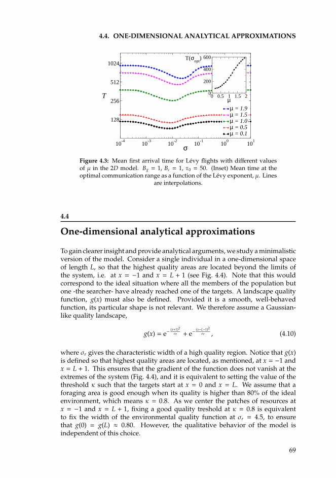
4.4. ONE-DIMENSIONAL ANALYTICAL APPROXIMATIONS
10-4
10-3
10-2
10-1
100
101
σ
128
256
512
1024
T
µ = 1.9µ = 1.5µ = 1.0µ = 0.5µ = 0.1
0 0.5 1 1.5 2µ
0
200
400
600T(σopt
)
Figure 4.3: Mean first arrival time for Levy flights with different valuesof µ in the 2D model. Bg = 1, Bc = 1, τ0 = 50. (Inset) Mean time at theoptimal communication range as a function of the Levy exponent, µ. Lines
are interpolations.
4.4
One-dimensional analytical approximations
To gain clearer insight and provide analytical arguments, we study a minimalisticversion of the model. Consider a single individual in a one-dimensional spaceof length L, so that the highest quality areas are located beyond the limits ofthe system, i.e. at x = −1 and x = L + 1 (see Fig. 4.4). Note that this wouldcorrespond to the ideal situation where all the members of the population butone -the searcher- have already reached one of the targets. A landscape qualityfunction, g(x) must also be defined. Provided it is a smooth, well-behavedfunction, its particular shape is not relevant. We therefore assume a Gaussian-like quality landscape,
g(x) = e−(x+1)2
σr + e−(x−L−1)2
σr , (4.10)
where σr gives the characteristic width of a high quality region. Notice that g(x)is defined so that highest quality areas are located, as mentioned, at x = −1 andx = L + 1. This ensures that the gradient of the function does not vanish at theextremes of the system (Fig. 4.4), and it is equivalent to setting the value of thethreshold κ such that the targets start at x = 0 and x = L. We assume that aforaging area is good enough when its quality is higher than 80% of the idealenvironment, which means κ = 0.8. As we center the patches of resources atx = −1 and x = L + 1, fixing a good quality treshold at κ = 0.8 is equivalentto fix the width of the environmental quality function at σr = 4.5, to ensurethat g(0) = g(L) ≈ 0.80. However, the qualitative behavior of the model isindependent of this choice.
69

CHAPTER 4. OPTIMAL SEARCH IN INTERACTING POPULATIONS
τ+(i)
0 1 i... L...
Caller
SearcherResourcesResources
Callerτ−(i)
Figure 4.4: Scheme of the simple version of the model.
Finally, for the pairwise communication function we choose the functions definedin Eq. (4.9) with p = 2 again. The combination of local and nonlocal informationgives the total available information for the searcher, R(x) = Bgg(x) + BcS(x).
To obtain analytical results, we work in the following on a discrete space. Thestochastic particle dynamics equivalent to Eq. (4.1) considers left and right jump-ing rates which are defined for every individual using the total informationfunction,
τ±(x) = max(τ0 +
R(x ± h) − R(x)h
, α
), (4.11)
where α is a small positive constant to avoid negative rates that has been givenan arbitrary value (α = 10−4), and h is the spatial discretization (h = 1). Finally,τ0 is the jumping rate of an individual in absence of information, and it is relatedto the diffusion component of the dynamics of Eq. (4.1). Given the transitionrates of Eq. (4.11), the movement with a higher gain of information has a higherrate, and therefore a larger probability of taking place.
The simplest situation, which allows an analytical treatment of the problem, isto consider only N = 3 individuals. Two of them are located in the top qualityareas just beyond the frontiers of the system limit, x = −1 and x = L + 1, and theother one is still searching for a target. Under these considerations, using theenvironmental quality function defined in Eq. (4.10), and the pairwise potentialof Eq. (4.9), the total available information for the searcher is
R(x; σ,L) = Bg
(e−
(x+1)2
σr + e−(x−L−1)2
σr
)+ BC
(e−
(x−L−1)2
σ + e−(x+1)2
σ
). (4.12)
As it was done in Sec. 4.2, the efficiency of the search process is measured interms of the first arrival time at one of the high quality areas, either at x = 0or x = L, starting from x0 = L/2. From the definition of the transition rates inEq. (4.11), τ+(L − 1) τ−(L), and equivalently τ−(1) τ+(0). This means thatat both extremes of the system, the rate at which particles arrive is much higherthan the rate at which they leave, so particles do not move when they arrive inthe top quality areas. This allows us to consider both extremes x = 0 and x = Lof the system as absorbing, and the first arrival time may be obtained from theflux of presence probability of the searcher there [Redner, 2001]
〈T(σ)〉 =∫ ∞
0t(∂P(0, t)∂t
+∂P(L, t)∂t
)dt. (4.13)
70
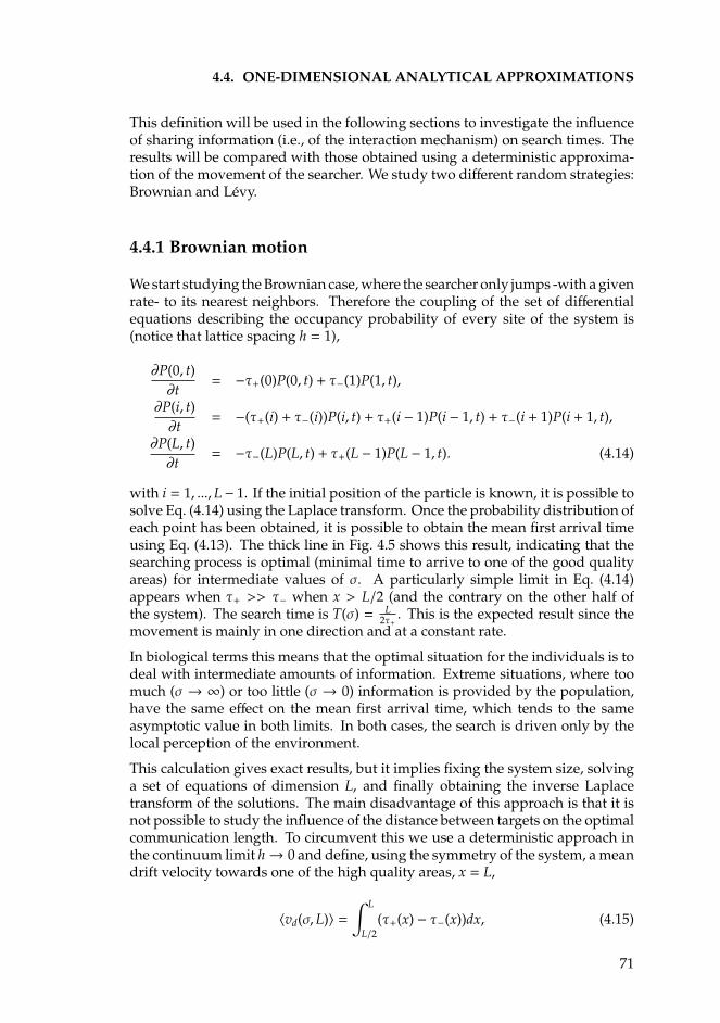
4.4. ONE-DIMENSIONAL ANALYTICAL APPROXIMATIONS
This definition will be used in the following sections to investigate the influenceof sharing information (i.e., of the interaction mechanism) on search times. Theresults will be compared with those obtained using a deterministic approxima-tion of the movement of the searcher. We study two different random strategies:Brownian and Levy.
4.4.1 Brownian motion
We start studying the Brownian case, where the searcher only jumps -with a givenrate- to its nearest neighbors. Therefore the coupling of the set of differentialequations describing the occupancy probability of every site of the system is(notice that lattice spacing h = 1),
∂P(0, t)∂t
= −τ+(0)P(0, t) + τ−(1)P(1, t),
∂P(i, t)∂t
= −(τ+(i) + τ−(i))P(i, t) + τ+(i − 1)P(i − 1, t) + τ−(i + 1)P(i + 1, t),
∂P(L, t)∂t
= −τ−(L)P(L, t) + τ+(L − 1)P(L − 1, t). (4.14)
with i = 1, ..., L− 1. If the initial position of the particle is known, it is possible tosolve Eq. (4.14) using the Laplace transform. Once the probability distribution ofeach point has been obtained, it is possible to obtain the mean first arrival timeusing Eq. (4.13). The thick line in Fig. 4.5 shows this result, indicating that thesearching process is optimal (minimal time to arrive to one of the good qualityareas) for intermediate values of σ. A particularly simple limit in Eq. (4.14)appears when τ+ >> τ− when x > L/2 (and the contrary on the other half ofthe system). The search time is T(σ) = L
2τ+. This is the expected result since the
movement is mainly in one direction and at a constant rate.
In biological terms this means that the optimal situation for the individuals is todeal with intermediate amounts of information. Extreme situations, where toomuch (σ → ∞) or too little (σ → 0) information is provided by the population,have the same effect on the mean first arrival time, which tends to the sameasymptotic value in both limits. In both cases, the search is driven only by thelocal perception of the environment.
This calculation gives exact results, but it implies fixing the system size, solvinga set of equations of dimension L, and finally obtaining the inverse Laplacetransform of the solutions. The main disadvantage of this approach is that it isnot possible to study the influence of the distance between targets on the optimalcommunication length. To circumvent this we use a deterministic approach inthe continuum limit h→ 0 and define, using the symmetry of the system, a meandrift velocity towards one of the high quality areas, x = L,
〈vd(σ,L)〉 =∫ L
L/2(τ+(x) − τ−(x))dx, (4.15)
71
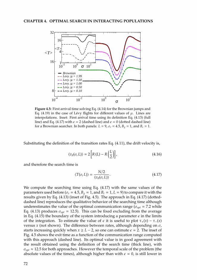
CHAPTER 4. OPTIMAL SEARCH IN INTERACTING POPULATIONS
10-4
10-2
100
102
σ
8
16
32
<T>
BrownianLevy. µ = 1.99Levy. µ = 1.50Levy. µ = 1.00Levy. µ = 0.50Levy. µ = 0.10
10-2
100
102σ
1
4
16
<T>
Figure 4.5: First arrival time solving Eq. (4.14) for the Brownian jumps andEq. (4.19) in the case of Levy flights for different values of µ. Lines areinterpolations. Inset: First arrival time using its definition Eq. (4.13) (fullline) and Eq. (4.17) with ε = 2 (dashed line) and ε = 0 (dotted dashed line)for a Brownian searcher. In both panels: L = 9, σr = 4.5, Bg = 1, and Bc = 1.
Substituting the definition of the transition rates Eq. (4.11), the drift velocity is,
〈vd(σ,L)〉 = 2[R (L) − R
(L2
)], (4.16)
and therefore the search time is
〈T(σ,L)〉 = N/2〈vd(σ,L)〉 . (4.17)
We compute the searching time using Eq. (4.17) with the same values of theparameters used before (σr = 4.5, Bg = 1, and Bc = 1, L = 9) to compare it with theresults given by Eq. (4.13) (inset of Fig. 4.5). The approach in Eq. (4.17) (dotted-dashed line) reproduces the qualitative behavior of the searching time althoughunderestimates the value of the optimal communication range (σopt = 7.2 whileEq. (4.13) produces σopt = 12.5). This can be fixed excluding from the averagein Eq. (4.15) the boundary of the system introducing a parameter ε in the limitsof the integration. To estimate the value of ε it is useful to plot τ+(x) − τ−(x)versus x (not shown). The difference between rates, although depending on σ,starts increasing quickly when x ≥ L − 2, so one can estimate ε = 2. The inset ofFig. 4.5 shows the exit time as a function of the communication range computedwith this approach (dashed line). Its optimal value is in good agreement withthe result obtained using the definition of the search time (thick line), withσopt ≈ 12.5 for both approaches. However the temporal scale of the problem (theabsolute values of the times), although higher than with ε = 0, is still lower in
72

4.4. ONE-DIMENSIONAL ANALYTICAL APPROXIMATIONS
101
102
103
104
L
101
102
103
σ1/2
Numerical solution Eq. (12)
Regression L0.93
opt
Figure 4.6: Scaling of the optimal communication range parameter withthe distance between targets (system size in the 1D simple model).
this calculation. Results for ε = 2 correspond to the dashed line in the inset ofFig. 4.5.
Regardless of the value of ε used in the average, this approximation underesti-mates the temporal scale of the problem (the absolute values of the times). Thisis because it is assumed that the searcher follows a deterministic movement tothe target neglecting any fluctuation that may slow the process.
Finally, increasing σ beyond its optimal value, there is a maximum for the searchtime for any of the approaches. For these values of the communication range,the nonlocal information at the middle of the system coming from both targetsis higher than in the extremes and thus there is a bias to the middle in themovement of the searcher. This small effect, that vanishes when σ increasesand the information tends to be constant in the whole system, seems to be anartifact of the particular arrangement of the simplified 1D system, and doesnot seem relevant for any real-world consideration of this kind of model. Inaddition, it does not substantially affect the dynamics because local perceptionof the environment pushes the individual towards one of the targets.
Finally, within this deterministic approximation, besides studying larger systemswith no additional computational cost, it is possible to obtain the optimal valueof the interaction range parameter, σopt:
(∂T∂σ
)σ=σopt
= 0, (4.18)
which has to be solved numerically for different sizes of the system. The typicaloptimal communication scale defined by σ1/p, (i.e., by σ1/2 since p = 2) growsapproximately linearly with the distance between targets in the asymptotic limit.Using a regression of the results obtained from the integration of Eq. (4.18) yieldsan exponent σ1/2
opt ∝ L0.93 for L 1 (Fig. 4.6).
73
CHAPTER 4. OPTIMAL SEARCH IN INTERACTING POPULATIONS
4.4.2 Levy flights.
Proceeding as in the case of Brownian motion, considering a Levy searcher theset of equations for the probability of occupancy is
∂P(0, t)∂t
=
L∑j=1
τ−( j)B jP( j, t) − τ+(0)P(0, t)
BL +
L−1∑j=1
A j
,∂P(i, t)∂t
=
i−1∑j=0
τ+( j)Ai− jP( j, t) +L∑
j=i+1
τ−( j)A j−iP( j, t) −
τ−(i)P(i, t)
Bi +
i−1∑j=1
A j
− τ+(i)P(i, t)
BL−i +
L−i−1∑j=1
A j
,∂P(L, t)∂t
=
L−1∑j=0
τ+( j)BL− jP( j, t) − τ−(L)P(L, t)
BL +
L−1∑j=1
A j
,(4.19)
with i = 1, . . . , L − 1.
We assume that if a jump of length in between j − 1 and j takes place, theindividual gets the position j. To this aim, the coefficients A j enter in the set of
equations (4.19) and are defined as A j =∫ j
j−1Ψµ(l)dl. They give the probabilityof a jump of length between j−1 and j to happen. The coefficients B j are definedas B j =
∫ ∞j−1Ψµ(l)dl, to take into account that the searcher stops if it arrives to a
target. This introduces a cutoff in the jumping length distribution Eq. (4.7).
Given the size of the system, L, which fixes the dimension of the system ofequations (4.19), it is possible to obtain an analytical solution for the occupancyprobabilities and the mean arrival time to the targets using Eq. (4.13). This isshown in Fig. 4.5, where the Brownian limit is recovered when µ→ 2. It is alsoobserved that when long jumps are frequent the search is much faster, althoughthe gain in search efficiency due to the communication mechanisms is lowerclose to the ballistic limit (i.e., µ→ 0). This will be explained later in Sec. 4.6.
Similarly to the Brownian case, a particularly simple limit in Eq. (4.19) appearswhen τ+ >> τ− for x > L/2 (and the contrary on the other half of the system).The search time is
T(x = L, σ) ∝ 1τ+,
where the proportionality constant is a combination of the coefficients Ai thatdepends on the size of the system.
74
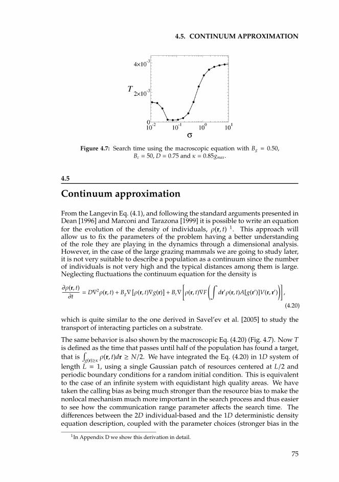
4.5. CONTINUUM APPROXIMATION
Figure 4.7: Search time using the macroscopic equation with Bg = 0.50,Bc = 50, D = 0.75 and κ = 0.85gmax.
4.5
Continuum approximation
From the Langevin Eq. (4.1), and following the standard arguments presented inDean [1996] and Marconi and Tarazona [1999] it is possible to write an equationfor the evolution of the density of individuals, ρ(r, t) 1. This approach willallow us to fix the parameters of the problem having a better understandingof the role they are playing in the dynamics through a dimensional analysis.However, in the case of the large grazing mammals we are going to study later,it is not very suitable to describe a population as a continuum since the numberof individuals is not very high and the typical distances among them is large.Neglecting fluctuations the continuum equation for the density is
∂ρ(r, t)∂t
= D∇2ρ(r, t) + Bg∇[ρ(r, t)∇g(r)
]+ Bc∇
[ρ(r, t)∇F
(∫dr′ρ(r, t)A[g(r′)]V(r, r′)
)],
(4.20)
which is quite similar to the one derived in Savel’ev et al. [2005] to study thetransport of interacting particles on a substrate.
The same behavior is also shown by the macroscopic Eq. (4.20) (Fig. 4.7). Now Tis defined as the time that passes until half of the population has found a target,that is
∫g(r)≥κ ρ(r, t)dr ≥ N/2. We have integrated the Eq. (4.20) in 1D system of
length L = 1, using a single Gaussian patch of resources centered at L/2 andperiodic boundary conditions for a random initial condition. This is equivalentto the case of an infinite system with equidistant high quality areas. We havetaken the calling bias as being much stronger than the resource bias to make thenonlocal mechanism much more important in the search process and thus easierto see how the communication range parameter affects the search time. Thedifferences between the 2D individual-based and the 1D deterministic densityequation description, coupled with the parameter choices (stronger bias in the
1In Appendix D we show this derivation in detail.
75
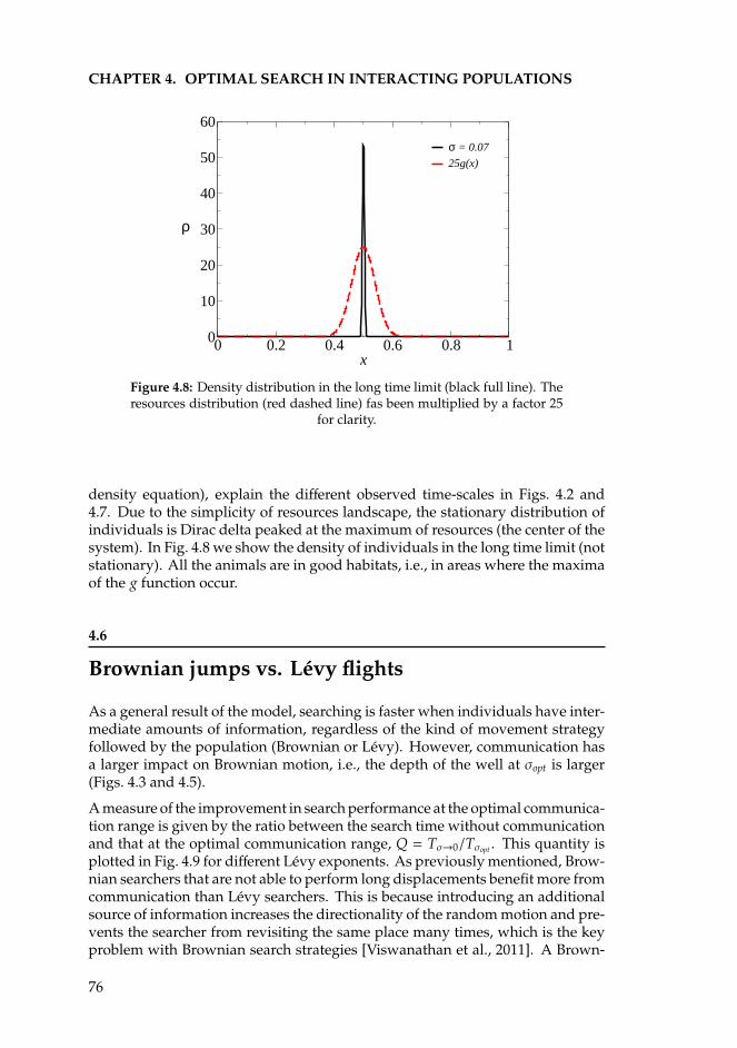
CHAPTER 4. OPTIMAL SEARCH IN INTERACTING POPULATIONS
0 0.2 0.4 0.6 0.8 1x
0
10
20
30
40
50
60
ρ
σ = 0.07
25g(x)
Figure 4.8: Density distribution in the long time limit (black full line). Theresources distribution (red dashed line) fas been multiplied by a factor 25
for clarity.
density equation), explain the different observed time-scales in Figs. 4.2 and4.7. Due to the simplicity of resources landscape, the stationary distribution ofindividuals is Dirac delta peaked at the maximum of resources (the center of thesystem). In Fig. 4.8 we show the density of individuals in the long time limit (notstationary). All the animals are in good habitats, i.e., in areas where the maximaof the g function occur.
4.6
Brownian jumps vs. Levy flights
As a general result of the model, searching is faster when individuals have inter-mediate amounts of information, regardless of the kind of movement strategyfollowed by the population (Brownian or Levy). However, communication hasa larger impact on Brownian motion, i.e., the depth of the well at σopt is larger(Figs. 4.3 and 4.5).
A measure of the improvement in search performance at the optimal communica-tion range is given by the ratio between the search time without communicationand that at the optimal communication range, Q = Tσ→0/Tσopt . This quantity isplotted in Fig. 4.9 for different Levy exponents. As previously mentioned, Brow-nian searchers that are not able to perform long displacements benefit more fromcommunication than Levy searchers. This is because introducing an additionalsource of information increases the directionality of the random motion and pre-vents the searcher from revisiting the same place many times, which is the keyproblem with Brownian search strategies [Viswanathan et al., 2011]. A Brown-
76
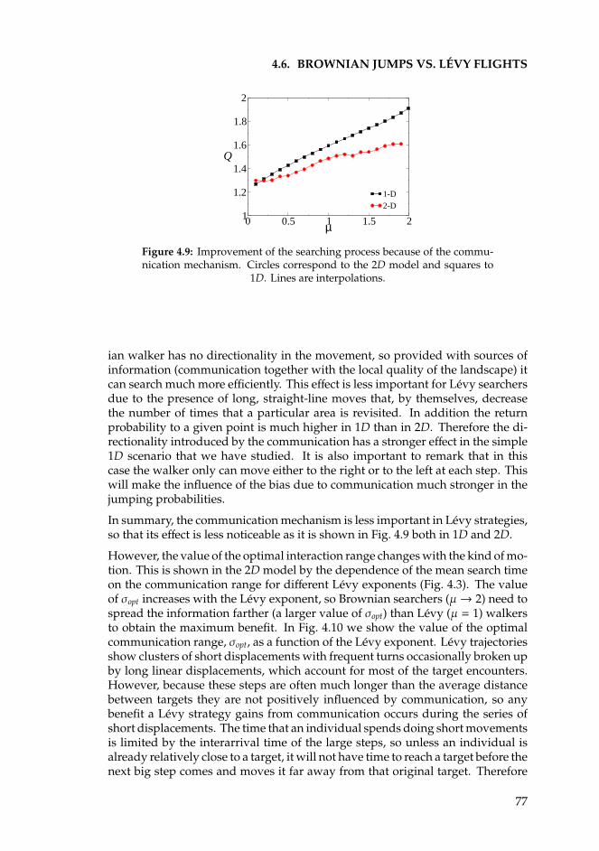
4.6. BROWNIAN JUMPS VS. LEVY FLIGHTS
0 0.5 1 1.5 2µ1
1.2
1.4
1.6
1.8
2
Q
1-D2-D
Figure 4.9: Improvement of the searching process because of the commu-nication mechanism. Circles correspond to the 2D model and squares to
1D. Lines are interpolations.
ian walker has no directionality in the movement, so provided with sources ofinformation (communication together with the local quality of the landscape) itcan search much more efficiently. This effect is less important for Levy searchersdue to the presence of long, straight-line moves that, by themselves, decreasethe number of times that a particular area is revisited. In addition the returnprobability to a given point is much higher in 1D than in 2D. Therefore the di-rectionality introduced by the communication has a stronger effect in the simple1D scenario that we have studied. It is also important to remark that in thiscase the walker only can move either to the right or to the left at each step. Thiswill make the influence of the bias due to communication much stronger in thejumping probabilities.
In summary, the communication mechanism is less important in Levy strategies,so that its effect is less noticeable as it is shown in Fig. 4.9 both in 1D and 2D.
However, the value of the optimal interaction range changes with the kind of mo-tion. This is shown in the 2D model by the dependence of the mean search timeon the communication range for different Levy exponents (Fig. 4.3). The valueof σopt increases with the Levy exponent, so Brownian searchers (µ→ 2) need tospread the information farther (a larger value of σopt) than Levy (µ = 1) walkersto obtain the maximum benefit. In Fig. 4.10 we show the value of the optimalcommunication range, σopt, as a function of the Levy exponent. Levy trajectoriesshow clusters of short displacements with frequent turns occasionally broken upby long linear displacements, which account for most of the target encounters.However, because these steps are often much longer than the average distancebetween targets they are not positively influenced by communication, so anybenefit a Levy strategy gains from communication occurs during the series ofshort displacements. The time that an individual spends doing short movementsis limited by the interarrival time of the large steps, so unless an individual isalready relatively close to a target, it will not have time to reach a target before thenext big step comes and moves it far away from that original target. Therefore
77
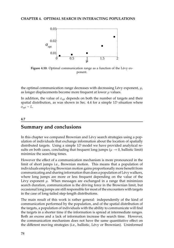
CHAPTER 4. OPTIMAL SEARCH IN INTERACTING POPULATIONS
0 0.5 1 1.5 2µ
0.01
0.02
0.03
σopt
Figure 4.10: Optimal communication range as a function of the Levy ex-ponent.
the optimal communication range decreases with decreasing Levy exponent, µ,as longer displacements become more frequent at lower µ values.
In addition, the value of σopt depends on both the number of targets and theirspatial distribution, as was shown in Sec. 4.4 for a simple 1D situation whereσopt ∼ L.
4.7
Summary and conclusions
In this chapter we compared Brownian and Levy search strategies using a pop-ulation of individuals that exchange information about the location of spatiallydistributed targets. Using a simple 1D model we have provided analytical re-sults on both cases, concluding that frequent long jumps (µ → 0, ballistic limit)minimize the searching times.
However the effect of a communication mechanism is more pronounced in thelimit of short jumps i.e., Brownian motion. This means that a population ofindividuals employing Brownian motion gains proportionally more benefit fromcommunicating and sharing information than does a population of Levy walkers,where long jumps are more or less frequent depending on the value of theLevy exponent µ. When messages are exchanged in a range that minimizessearch duration, communication is the driving force in the Brownian limit, butoccasional long jumps are still responsible for most of the encounters with targetsin the case of long-tailed step-length distributions.
The main result of this work is rather general: independently of the kind ofcommunication performed by the population, and of the spatial distribution ofthe targets, a population of individuals with the ability to communicate will findthe targets in a shorter time if the information is spread at intermediate ranges.Both an excess and a lack of information increase the search time. However,the communication mechanism does not have the same quantitative effect onthe different moving strategies (i.e., ballistic, Levy or Brownian). Uninformed
78

4.7. SUMMARY AND CONCLUSIONS
Brownian individuals perform a random movement revisiting the same positionmany times, so having an external source of information introduces directionalityon the movement, decreasing the number of times that a point in the space isvisited. In the case of Levy and ballistic strategies (µ → 0), communication isless noticeable because individuals are able to do long jumps. This is alreadya source of directionality that prevents individuals from revisiting the samepoints in space many times, and thus weakening the effect of the directionalityintroduced by communication.
79

CHAPTER 5Foraging in Procapra gutturosa
In this chapter we show an application of the model presented in Chapter 4 to theparticular case of acoustic communication among Mongolian gazelles (Procapragutturosa), for which data are available, searching for good habitat areas. UsingMonte Carlo simulations, our results point out that the search is optimal (i.e.the mean first hitting time among searchers is minimum) at intermediate scalesof communication. We also present this result in terms of the frequency ofthe sounds, showing a good agreement with field measurements of the soundsemitted by these gazelles in the wild. The formation of groups in the populationsis also studied.
5.1
Introduction
Many living organisms, including bacteria [Liu and Passino, 2002], insects, andmammals [Zuberbuhler et al., 1997; McComb et al., 2003] communicate for a va-riety of reasons including facilitation of social cohesion [Cap et al., 2008; Pfefferleand Fischer, 2006], defense against predators [Zuberbuhler, 2001], maintenanceof territories [Slater et al., 1994; Frey et al., 2007], and to pool information onresource locations when no single individual is sufficiently knowledgeable [vonFrisch, 1967; Hoare et al., 2004; Berdahl et al., 2013; Simons, 2004; Torney et al.,2009b]. Communication among individuals frequently leads to group forma-tion [Eftimie et al., 2007], which often has clear direct benefits such as reducingindividual vulnerability to predators. Such strategies may, however, also haveimportant incidental benefits. For example, an individual that has found a goodforaging patch might try to attract conspecifics to reduce its risk of predation, butalso provides its conspecifics with information on the location of good forage,thus increasing the foraging efficiency of those responding to the call.
We apply a specialized version of the model introduced in Chapter 4 to the par-ticular case of acoustic communication among Mongolian gazelle, the dominantwild herbivore in the Eastern steppe of Mongolia (Fig. 5.1a) among 14 species
81
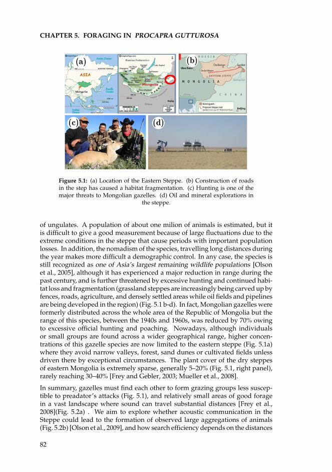
CHAPTER 5. FORAGING IN PROCAPRA GUTTUROSA
Figure 5.1: (a) Location of the Eastern Steppe. (b) Construction of roadsin the step has caused a habitat fragmentation. (c) Hunting is one of themajor threats to Mongolian gazelles. (d) Oil and mineral explorations in
the steppe.
of ungulates. A population of about one milion of animals is estimated, but itis difficult to give a good measurement because of large fluctuations due to theextreme conditions in the steppe that cause periods with important populationlosses. In addition, the nomadism of the species, travelling long distances duringthe year makes more difficult a demographic control. In any case, the species isstill recognized as one of Asia’s largest remaining wildlife populations [Olsonet al., 2005], although it has experienced a major reduction in range during thepast century, and is further threatened by excessive hunting and continued habi-tat loss and fragmentation (grassland steppes are increasingly being carved up byfences, roads, agriculture, and densely settled areas while oil fields and pipelinesare being developed in the region) (Fig. 5.1 b-d). In fact, Mongolian gazelles wereformerly distributed across the whole area of the Republic of Mongolia but therange of this species, between the 1940s and 1960s, was reduced by 70% owingto excessive official hunting and poaching. Nowadays, although individualsor small groups are found across a wider geographical range, higher concen-trations of this gazelle species are now limited to the eastern steppe (Fig. 5.1a)where they avoid narrow valleys, forest, sand dunes or cultivated fields unlessdriven there by exceptional circumstances. The plant cover of the dry steppesof eastern Mongolia is extremely sparse, generally 5–20% (Fig. 5.1, right panel),rarely reaching 30–40% [Frey and Gebler, 2003; Mueller et al., 2008].
In summary, gazelles must find each other to form grazing groups less suscep-tible to preadator’s attacks (Fig. 5.1), and relatively small areas of good foragein a vast landscape where sound can travel substantial distances [Frey et al.,2008](Fig. 5.2a) . We aim to explore whether acoustic communication in theSteppe could lead to the formation of observed large aggregations of animals(Fig. 5.2b) [Olson et al., 2009], and how search efficiency depends on the distances
82
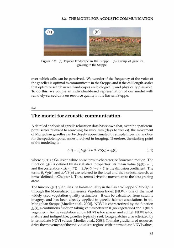
5.2. THE MODEL FOR ACOUSTIC COMMUNICATION
Figure 5.2: (a) Typical landscape in the Steppe. (b) Group of gazellesgrazing in the Steppe.
over which calls can be perceived. We wonder if the frequency of the voice ofthe gazelles is optimal to communicate in the Steppe, and if the call length-scalesthat optimize search in real landscapes are biologically and physically plausible.To do this, we couple an individual-based representation of our model withremotely-sensed data on resource quality in the Eastern Steppe.
5.2
The model for acoustic communication
A detailed analysis of gazelle relocation data has shown that, over the spatiotem-poral scales relevant to searching for resources (days to weeks), the movementof Mongolian gazelles can be closely approximated by simple Brownian motionfor the spatiotemporal scales involved in foraging. Therefore, the starting pointof the modeling is
ri(t) = Bg∇g(ri) + BC∇S(ri) + ηi(t), (5.1)
where ηi(t) is a Gaussian white noise term to characterize Brownian motion. Thefunction ηi(t) is defined by its statistical properties: its mean value 〈ηi(t)〉 = 0,and the correlation 〈ηi(t)η j(t′)〉 = 2Dδi jδ(t− t′). D is the diffusion coefficient. Theterms Bg∇g(ri) and BC∇S(ri) are referred to the local and the nonlocal search, asit was defined in Chapter 4. These terms drive the movement to the best grazingareas.
The function g(r) quantifies the habitat quality in the Eastern Steppe of Mongoliathrough the Normalized Difference Vegetation Index (NDVI), one of the mostwidely used vegetation quality estimators. It can be calculated from satelliteimagery, and has been already applied to gazelle habitat associations in theMongolian Steppe [Mueller et al., 2008]. NDVI is characterized by the functiongd(r), a continuous function taking values between 0 (no vegetation) and 1 (fullyvegetated). As the vegetation at low NDVI is too sparse, and at high NDVI is toomature and indigestible, gazelles typically seek forage patches characterized byintermediate NDVI values [Mueller et al., 2008]. To make gradients of resourcesdrive the movement of the individuals to regions with intermediate NDVI values,
83
CHAPTER 5. FORAGING IN PROCAPRA GUTTUROSA
we apply to the data a linear transformation:
f (x) =
gd(r) if gd(r) < 0.51 − gd(r) if gd(r) ≥ 0.5 (5.2)
The new function g(r) defines a resources landscape with values between 0and 0.5, where 0 represents both fully vegetated and no vegetation (i.e., lowquality forage). We study a subregion with an extension of around 23000 km2
(Coordinates: 46.50°N, 114.15°E; 46.50°N, 116.80°E; 47.65°N, 114.15°E; 47.65°N,116.80°E) and assume that the resources remain constant in time during thesearch. It is crucial now to properly choose the perception function in order torealistically model the case of gazelles performing acoustic communication. It iswell known that the sensitivity of the response of the ear does not follow a linearscale, but approximately a logarithmic one. That is why the bel and the decibelare quite suitable to describe the acoustic perception of a listener. Therefore wechoose an acoustic perception function of the form
S(ri) = 10 log10
∑N
j=1, j,i A[g(r j)]V(ri, r j)
I0
, (5.3)
where F is taken as a logarithmic function. The sound calling of j, V(r, r j), playsthe role of a two body interaction potential, and I0 is the low perception threshold.We take the value of a human ear, I0 = 10−12 W m−2, which is similar for mostother mammals [Fletcher, 1992], and in any case, is just a reference value onwhich our results will not depend. The interaction potential mimicking acousticcommunication is
V(ri, r j) =P0
4πe−γ|ri−r j |
|r − r j|2, (5.4)
considering that sound from an acoustic source attenuates in space mainly dueto the atmospheric absorption (exponential term), and the spherical spreadingof the intensity (4πr−2 contribution), and neglecting secondary effects [Naguiband Wiley, 2001]. P0 may be understood as the power of the sound at a distanceof 1 m from the source. According to Stoke’s law of sound attenuation [Fletcher,1992], the absorption coefficient, γ, is given by
γ =16π2ην2
3ρv3 , (5.5)
where η is the viscosity of the air, ρ its density, v the propagation velocity of theacoustic signal (which depends on the temperature and the humidity), and ν itsfrequency. We work under environmental conditions of T = 20oC, and relativehumidity of HR = 50%, which are quite close to the corresponding empiricalvalues for the summer months from the Baruun-Urt (Mongolia) weather station,averaged over the last 4 years. These values give an absorption coefficient ofγ ≈ 10−10ν2 m−1. The inverse of the absorption coefficient, γ−1, gives the typicallength scale for the communication at each frequency, and thus plays the samerole as the standard deviation, σ, did in the Gaussian interaction used in the
84
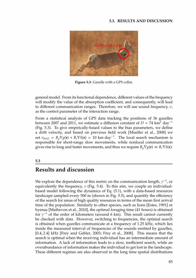
5.3. RESULTS AND DISCUSSION
Figure 5.3: Gazelle with a GPS collar.
general model. From its functional dependence, different values of the frequencywill modify the value of the absorption coefficient, and consequently, will leadto different communication ranges. Therefore, we will use sound frequency, ν,as the control parameter of the interaction range.
From a statistical analysis of GPS data tracking the positions of 36 gazellesbetween 2007 and 2011, we estimate a diffusion constant of D = 74 km2 day−1
(Fig. 5.3). To give empirically-based values to the bias parameters, we definea drift velocity, and based on previous field work [Mueller et al., 2008] weset vdri f t = Bg∇g(r) + Bc∇S(r) = 10 km day−1. The local search mechanism isresponsible for short-range slow movements, while nonlocal communicationgives rise to long and faster movements, and thus we require Bg∇g(r) Bc∇S(r).
5.3
Results and discussion
We explore the dependence of this metric on the communication length, γ−1, orequivalently the frequency, ν (Fig. 5.4). To this aim, we couple an individual-based model following the dynamics of Eq. (5.1), with a data-based resourceslandscape sampled every 500 m (shown in Fig. 5.5), and quantify the efficiencyof the search for areas of high quality resources in terms of the mean first arrivaltime of the population. Similarly to other species, such as lions [Estes, 1991] orhyenas [Mathevon et al., 2010], the optimal foraging time (41 hours) is obtainedfor γ−1 of the order of kilometers (around 6 km). This result cannot currentlybe checked with data. However, switching to frequencies, the optimal searchis obtained when gazelles communicate at a frequency of 1.25 kHz, which liesinside the measured interval of frequencies of the sounds emitted by gazelles,[0.4, 2.4] kHz [Frey and Gebler, 2003; Frey et al., 2008]. This means that thesearch is optimal when the receiving individual has an intermediate amount ofinformation. A lack of information leads to a slow, inefficient search, while anoverabundance of information makes the individual to get lost in the landscape.These different regimes are also observed in the long time spatial distributions
85
CHAPTER 5. FORAGING IN PROCAPRA GUTTUROSA
10-2
10-1
100
101
Emiting frequency (kHz)
024487296
120144168192
Tim
e (h
ours
)4 km10 km
41
0.4 KHz 2.4 KHz
GAZELLE CALLINGRANGE
hours
Figure 5.4: Mean arrival time for 500 gazelles (averaged over 50 realizationswith different initial conditions). Parameter values: D = 74 km2 day−1,
Bg = 2.6 × 10⁻³ km3 day−1, Bc = 13 km2 day−1, κ = 0.70gmax.
(i.e. efficiency of the search in terms of quality) of the Fig. 5.5. For frequenciesout of the optimal range, either smaller (Fig. 5.5 top) or larger (Fig. 5.5 bottomright), some animals are still in low-quality areas at the end of the simulationperiod. At intermediate communication scales, ν = 1 kHz, (Fig. 5.5 bottom left)all of the animals end up in regions with the best resources, regardless of wherethey started from.
In summary, communication over intermediate scales results in faster search,and all the individuals form groups in areas of good resources. While this hasobvious advantages in terms of group defense and predator swamping, it willalso lead to rapid degradation of the forage (and thus habitat quality) at thoselocations. This is the problem of foraging influencing the patterns of vegetation,which could be treated in future investigations. Shorter-scale communicationimplies an almost individual search, which helps preserve local forage quality,but has clear disadvantages in terms of group defense strategies. On the otherhand, longer scales lead to the formation of big groups (faster degradation offoraging), and animals need more time to join a group, which has negativeconsequences against predation. Furthermore, acoustic communication scalessignificantly larger than the optimal scale for foraging efficiency identified herewould be biologically implausible, even if ultimate group size (and not rate ofgroup formation) was the most important aspect of an antipredation strategy.
Our study clarifies some questions on the relationship between communicationand optimal search for resources. Our key result is that, in general, intermediatecommunication distances optimize search efficiency in terms of time and quality.Individuals are able to find the best quality resource patches regardless of wherethey start from, opening new questions about the distribution of individualsin heterogeneous landscapes. The existence of maximum search efficiency atintermediate communication ranges is robust to the choice of functional formof V(r), allowing the model to be generalized to many different ways of sharinginformation. Also considering different species on the model (preys and preda-
86
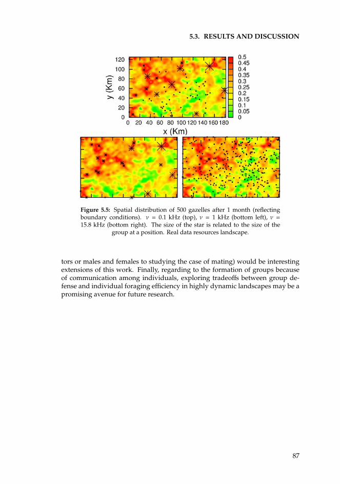
5.3. RESULTS AND DISCUSSION
Figure 5.5: Spatial distribution of 500 gazelles after 1 month (reflectingboundary conditions). ν = 0.1 kHz (top), ν = 1 kHz (bottom left), ν =15.8 kHz (bottom right). The size of the star is related to the size of the
group at a position. Real data resources landscape.
tors or males and females to studying the case of mating) would be interestingextensions of this work. Finally, regarding to the formation of groups becauseof communication among individuals, exploring tradeoffs between group de-fense and individual foraging efficiency in highly dynamic landscapes may be apromising avenue for future research.
87

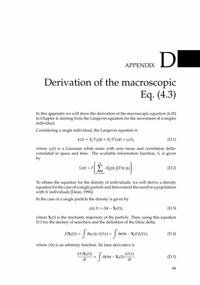
APPENDIX DDerivation of the macroscopic
Eq. (4.3)
In this appendix we will show the derivation of the macroscopic equation (4.20)in Chapter 4, starting from the Langevin equation for the movement of a singlesindividual.
Considering a single individual, the Langevin equation is
ri(t) = Bg∇g(r) + BC∇Si(r) + ηi(t), (D.1)
where ηi(t) is a Gaussian white noise with zero mean and correlation delta-correlated in space and time. The available information function, Si is givenby
Si(r) = F
N∑j=1, j,i
A[g(r j)]V(r, rj)
. (D.2)
To obtain the equation for the density of individuals, we will derive a densityequation for the case of a single particle and then extend the result to a populationwith N individuals [Dean, 1996].
In the case of a single particle the density is given by
ρ(r, t) = δ(r − Xi(t)), (D.3)
where Xi(t) is the stochastic trajectory of the particle. Then, using this equationD.3 for the density of searchers and the definition of the Dirac delta,
f (Xi(t)) =∫
drρi(r, t) f (x) =∫
drδ(r − Xi(t)) f (x), (D.4)
where f (r) is an arbitrary function. Its time derivative is
d f (Xi(t))dt
=
∫drδ(r − Xi(t))
d f (x)dt
. (D.5)
89
APPENDIX D. DERIVATION OF THE MACROSCOPIC EQ. (4.3)
Using the Ito’s formula Eq. (D.5) can be expanded,
d f (Xi(t))dt
=
∫drρi(r, t)
[D∇2 f (r) + Bg∇g(r)∇ f (r) + Bc∇Si(r)∇ f (r) + ∇ f (r)ηi(t)
], (D.6)
and then, rearranging and integrating by parts each term1,
d f (Xi(t))dt
=
∫dr f (r)
[D∇2ρi(r, t) + Bg∇
(ρi(r, t)∇g(r)
)]+
∫dr f (r)
[Bc∇
(ρi(r, t)∇Si(r)
)+ ∇(ρi(r, t)ηi(t))
]. (D.7)
On the other hand the time derivative of f (r) can be written as
d f (Xi(t))dt
=
∫dr f (r)∂t[ρi(r, t)]. (D.8)
As both Eq. (D.7) and (D.8) are true in the case of an arbitrary function, f (r), it ispossible to write:
∂ρi(r, t)∂t
= D∇2ρi(r, t) + Bg∇[ρi(r, t)∇g(r)
]+ Bc∇
[ρi(r, t)∇Si(r)
]+ ∇[ρi(r, t)ηi(t)].
(D.9)
Finally, we neglect the last stochastic term to get a deterministic approximationas Eq. (4.20).
1It is straightforward just choosing ∇ f (x) = dV in the integration by parts. In the case of thelaplacian term, we must integrate twice.
90
APPENDIX EVoronoi diagrams of the model.
The behavior of the model, resulting in optimal searches at intermediate com-munication ranges, can be explained in terms of Voronoi diagrams Okabe et al.[1992]. Consider every target as a seed that has associated a Voronoi cell formedby those points whose distance to that seed is less than or equal to its distanceto any other one (See Figure E.1 (top) for a distribution of the space in 5 Voronoicells for an initial distribution of particles with five targets (crosses)). The search-ing time will be minimized when the information coming from the individualslocated on one target covers the full associated Voronoi cell, but only that cell.In this situation, the searchers within that cell will receive information comingonly from that target and move towards it. σopt is the communication rangethat maximizes the gradient (approximately the smallest value of σ that makesthe calling function not vanishing) of the calling function at the frontiers of theVoronoi cells. Increasing the communication range provides individuals withinformation coming from different targets, and makes them get overwhelmedin the limit σ → ∞. This Voronoi construction may also help to explain theimprovement of the searching strategies because of sharing information. Thedifference between Brownian and Levy strategies can be seen in Figure E.1 (Bot-tom). They show the origin of the individuals that are at each target at the end ofa Levy (Left) and a Brownian search (Right) (i.e., in which Voronoi cell they wereat the beginning). In the case of Brownian individuals most of the particles atevery target were initially in its Voronoi cell. For Levy flights the long displace-ments mix the population in the stationary state (i.e., individuals at a target comefrom different cells). The communication mechanism is less important in Levystrategies, so that its effect is less noticeable and the encounters of individualswith targets are caused mainly by the long displacements.
91
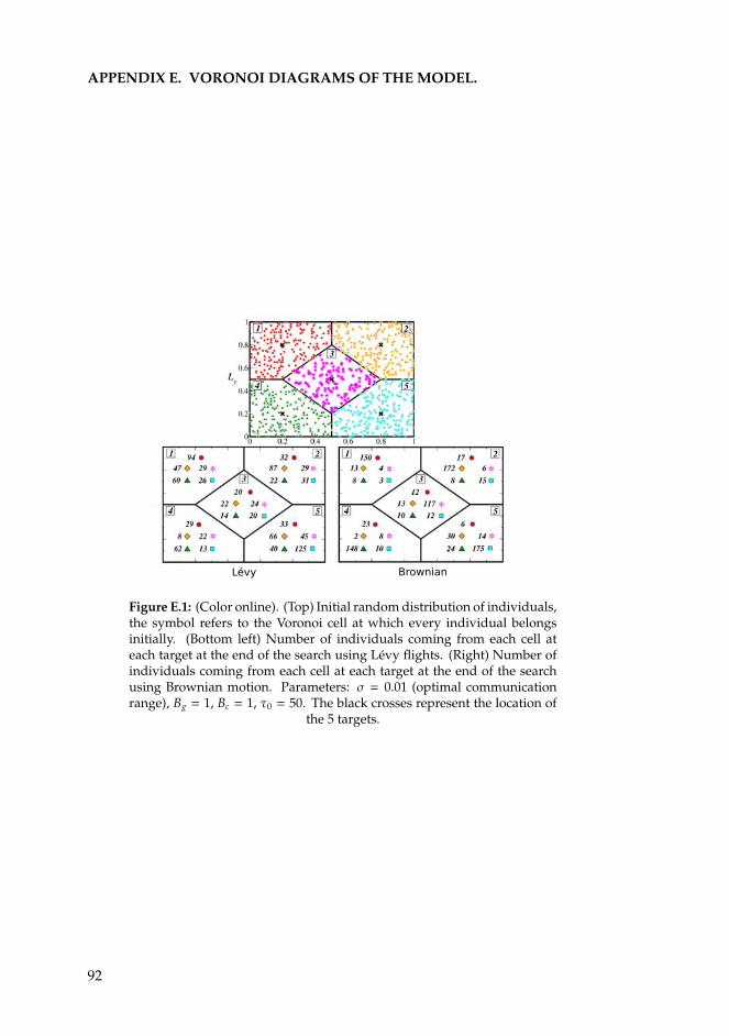
APPENDIX E. VORONOI DIAGRAMS OF THE MODEL.
Lévy Brownian
Figure E.1: (Color online). (Top) Initial random distribution of individuals,the symbol refers to the Voronoi cell at which every individual belongsinitially. (Bottom left) Number of individuals coming from each cell ateach target at the end of the search using Levy flights. (Right) Number ofindividuals coming from each cell at each target at the end of the searchusing Brownian motion. Parameters: σ = 0.01 (optimal communicationrange), Bg = 1, Bc = 1, τ0 = 50. The black crosses represent the location of
the 5 targets.
92
Part IV
Temporal fluctuations
Lars Onsager
(1903-1976)
Norwegian-born American physical chemist and theoretical
physicist, winner of the 1968 Nobel Prize in Chemistry. During
the 1940s, he studied the statistical-mechanical theory of phase
transitions in solids, deriving a mathematically elegant theory
which was enthusiastically received. He obtained the exact
solution for the two dimensional Ising model in zero field in
1944.
93

CHAPTER 6Temporal disorder in up-down
symmetric systems
In this chapter we study the effect of temporal fluctuations on systems withup-down symmetry through the behavior of the first-passage times. This isa relevant question in the modeling of ecosystems, since they are subject toenvironmental changing conditions. Therefore, it is important to have modelsthat include temporal disorder. We analyze two well-known families of phasetransitions in statistical physics —the Ising and the generalized voter universalityclasses— and scrutinize the consequences of placing them under fluctuatingglobal conditions. It is observed that the variability of the control parameterinduces in both classes “temporal Griffiths phases” (TGPs), characterized bybroad regions in the parameter space in which the mean first-passage times scalealgebraically with system size. In an ecological context, first-passage times arerelated to typical extinction times, and studying how they are affected by the sizeof the system (e.g. habitat fragmentation) is a problem of outmost relevance.
6.1
Introduction
Systems with up-down Z2 symmetry –including the Ising model– are paradig-matic in mathematical ecology. They allow to address a big variety of problemsranging from species competition [Clifford and Sudbury, 1973] and neutral the-ories of biodiversity [Durrett and Levin, 1996] to allele frequency in genetics[Baxter et al., 2007]. Some of them, such as the voter model, exhibit absorbingstates, a distinctive feature of nonequilibrium dynamics. Once these particularconfigurations are reached, the system cannot escape from them so they implythe presence of currents [Hinrichsen, 2000; Odor, 2004; Grinstein and Munoz,1996; Marro and Dickman, 2008].
Phase transitions into absorbing states are quite universal and they depend onfew general properties of the system, such as symmetries and its dimensionality,
95
CHAPTER 6. TEMPORAL DISORDER IN UP-DOWN SYMMETRICSYSTEMS
and are insensitive to the underlying microscopic properties. This universalitymakes possible to establish a classification of the phase transitions into differentclasses. Those systems exhibiting one absorbing state belong generically to thecalled Directed Percolation (DP) universality class and share the same set of crit-ical exponents and scaling functions. However, when there is some additionalsymmetry or conservation, the phase transition exhibits critical scaling differ-ing from DP. This is the case of systems with two symmetric absorbing states[Hinrichsen, 2000; Odor, 2004; Grinstein and Munoz, 1996; Marro and Dickman,2008], that show a phase transition usually referred as Generalized voter (GV).In an ecological context, this is a relevant class of models that can be used inmany situations with two equivalent species.
Analytical and numerical studies [Dornic et al., 2001; Droz et al., 2003; Al Hammalet al., 2005; Vazquez and Lopez, 2008; Russell and Blythe, 2011] have shown that,depending on some details such GV transition can split into two separate ones:an Ising-like transition in which the up-down symmetry is broken, and a secondDP-like transition below which the broken-symmetry phase collapses into thecorresponding absorbing state. In particular, a general stochastic theory, aimedat capturing the phenomenology of these systems, was proposed in Al Hammalet al. [2005]; depending on general features they may exhibit a DP, an Ising, or aGV transition.
When they try to mimick ecological systems, these models should not be isolatedbut, instead, affected by external conditions or by environmental fluctuations.The question of how external variability affects diversity, robustness, and evolu-tion of complex systems, is of outmost relevance in ecology. Take, for instance,the example of the neutral theory of biodiversity: if there are two Z2-symmetric(or neutral) species competing, what happens if depending on environmentalconditions one of the two species is favored at each time step in a symmetricway? Does such environmental variability enhance species coexistence or doesit hinder it? [Giles Leigh Jr., 1981; Vazquez et al., 2010; Borgogno et al., 2009].
Motivated by these questions, we study how basic properties of up-down sym-metric systems, such as response functions and first-passage times, are affectedby the presence of temporal disorder.
Some previous works have explored from a theoretical point of view the effectsof fluctuating global conditions in simple models that exhibit phase transitions[Jensen, 1996; Alonso and Munoz, 2001; Kamenev et al., 2008]. Recently, amodified version of the simplest representative of the DP class –i.e. the ContactProcess– equipped with temporal disorder was studied in Vazquez et al. [2011].In this model, the control parameter (birth probability) was taken to be a randomvariable, varying at each time unit. As the control parameter is allowed to takevalues above and below the transition point of the pure contact process, thesystem alternates between the tendencies to be active or absorbing. As shownin Vazquez et al. [2011] this dynamical frustration induces a logarithmic type offinite-size scaling at the transition point and generates a subregion in the activephase characterized by a generic algebraic scaling of the extinction times withsystem size. More strikingly, this subregion is also characterized by generic
96
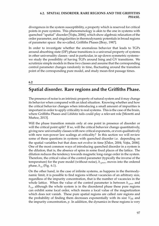
6.2. SPATIAL DISORDER. RARE REGIONS AND THE GRIFFITHSPHASE.
divergences in the system susceptibility, a property which is reserved for criticalpoints in pure systems. This phenomenology is akin to the one in systems withquenched “spatial” disorder [Vojta, 2006], which show algebraic relaxation of theorder parameter, and singularities in thermodynamic potentials in broad regionsof parameter space: the so-called, Griffiths Phases [Bray, 1987].
In order to investigate whether the anomalous behavior that leads to TGPsaround absorbing state (DP) phase transitions is a universal property of systemsin other universality classes –and in particular, in up-down symmetric systems–we study the possibility of having TGPs around Ising and GV transitions. Wescrutinize simple models in these two classes and assume that the correspondingcontrol parameter changes randomly in time, fluctuating around the transitionpoint of the corresponding pure model, and study mean-first passage times.
6.2
Spatial disorder. Rare regions and the Griffiths Phase.
The presence of noise is an intrinsic property of natural system and it may changeits behavior when compared with an ideal situation. Knowing whether and howthe critical behavior changes when introducing a small amount of impurities isimportant in order to apply criticality to real systems. This is the case of the brain,where Griffiths Phases and Lifshitz tails could play a relevant role [Moretti andMunoz, 2013].
Will the phase transition remain only at one point in presence of disorder orwill the critical point split? If so, will the critical behavior change quantitatively,giving new universality classes with new critical exponents, or even qualitativelywith new non-power law scalings at criticality? In this section we will reviewsome of these questions in systems with quenched disorder i.e. depending onthe spatial variables but that does not evolve in time [Odor, 2004; Vojta, 2006].One of the most common ways of introducing quenched disorder in a system isthe dilution, that is, the absence of spins in some fixed places of the lattice. Thedilution reduces the tendency towards magnetic long-range order in the system.Therefore, the critical value of the control parameter (typically the inverse of thetemperature) for the pure model (without noise), bc,pure, moves into the orderedphase, bc,q (Fig. 6.1).
On the other hand, in the case of infinite systems, as happens in the thermody-namic limit, it is possible to find regions without vacancies of an arbitrary size,regardless of the impurity concentration, that is the number of vacancies in thewhole lattice. When the value of the control parameter is between bc,pure andbc,q, although the whole system is in the disordered phase these pure regionscan exhibit some local order, which means a local value of the magnetizationwhich does not vanish. These pure spatial regions are called rare regions andthe probability of finding them decreases exponentially with its size VRR andthe impurity concentration, p. In addition, the dynamics in these regions is very
97
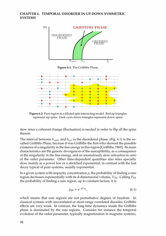
CHAPTER 6. TEMPORAL DISORDER IN UP-DOWN SYMMETRICSYSTEMS
m
b
PHASEDISORDERED
ORDEREDPHASE
bc,pure bc,q
GRIFFITHS PHASE
Figure 6.1: The Griffiths Phase.
Figure 6.2: Pure region in a diluted spin interacting model. Red up trianglesrepresent up spins. Dark cyan down triangles represent down spins.
slow since a coherent change (fluctuation) is needed in order to flip all the spinstherein.
The interval between bc,pure and bc,q, in the disordered phase, (Fig. 6.1) is the so-called Griffiths Phase, because it was Griffiths the first who showed the possibleexistence of a singularity in the free energy in this region [Griffiths, 1969]. Its maincharacteristics are the generic divergences of the susceptibility, as a consequenceof the singularity in the free energy, and an anomalously slow relaxation to zeroof the order parameter. Other time-dependent quantities also relax speciallyslow, mainly as a power law or a stretched exponential, in contrast with the fastdecay typical of pure systems, usually exponential.
In a given system with impurity concentration p, the probability of finding a rareregion decreases exponentially with its d-dimensional volume, VRR. Calling PRRthe probability of finding a rare region, up to constant factors, it is
pRR ∝ e−pVRR , (6.1)
which means that rare regions are not perturbative degrees of freedom. Inclassical systems with uncorrelated or short-range correlated disorder, Griffithseffects are very weak. In contrast, the long-time dynamics inside the Griffithsphase is dominated by the rare regions. Consider for instance the temporalevolution of the order parameter, typically magnetization in magnetic systems,
98
6.3. MEAN-FIELD THEORY OF Z2-SYMMETRIC MODELS WITHTEMPORAL DISORDER.
m. As its long time behavior is governed by rare regions, it is
m(t) ∝∫
dVRRPRRe−t/ξt(VRR), (6.2)
where ξt is the flipping time of a rare region, and increases exponentially withits size, so it is ξt(VRR) ∝ exp(bVRR). The integral in Eq. (6.2) can be solved usinga saddle-node integration to obtain the slow relaxation of the magentizationtypical of Griffiths Phases
m(t) ∝ t−φ, (6.3)
where φ is a non-universal exponent the varies in the Griffiths Phase.
6.3
Mean-field theory of Z2-symmetric models with tem-poral disorder.
Interacting particle models, such as ecosystems, evolve stochastically over time.A useful technique to study such systems is the mean-field (MF) approach, whichimplicitly assumes a well-mixed situation, where each particle can interact withany other, providing a sound approximation in high dimensional systems. Oneway in which the mean-field limit can be seen at work is by analyzing a fullyconnected network (FCN), where each node (particle) is directly connected toany other else, mimicking an infinite dimensional system.
In the models that we study here, states can be labeled with occupation-numbervariables ρi taking a value 1 if node i is occupied or 0 if it is empty, or alternativelyby spin variables Si = 2ρi − 1, with Si = ±1. Using these latter, the natural orderparameter is the magnetization per spin, defined as
m =1N
N∑i=1
Si, (6.4)
where N is the total number of particles in the system. Note that it is calledthe order parameter because it gives the degree of order in the system. Its valuevaries between−1 an 1, both of them corresponding to a fully ordered state, withthe intermediate value m = 0 reflects a disordered system with the same amountof spins up and down. The rate equation for the probability P(m, t) of havingmagnetization m at a given time t, is
P(m, t + 1/N) =ω+ (m − 2/N, b)
NP (m − 2/N, t) (6.5)
+ω− (m + 2/N, b)
NP (m + 2/N, t)
+
[1 − ω−(m, b)
N− ω+(m, b)
N
]P(m, t) + O(N−2),
99
CHAPTER 6. TEMPORAL DISORDER IN UP-DOWN SYMMETRICSYSTEMS
where ω±(m, b) are the transition probabilities from a state with magnetizationm to a state with magnetization m ± 2/N.
In the limit of N→∞ (dt→ 0) Eq. (6.5) becomes a Master equation (Sec. 1.1.1),
∂P(m, t)∂t
= ω+ (m − 2/N, b) P (m − 2/N, t) (6.6)
+ ω− (m + 2/N, b) P (m + 2/N, t)− [ω−(m, b) + ω+(m, b)] P(m, t) + O(N−2).
This describes a process in which a “spin” is randomly selected at every time-step (of length dt = 1/N), and inverted with a probability that depends on m andthe control parameter b. The allowed magnetization changes in an individualupdate, ∆m = ±2/N, are infinitesimally small in the N → ∞ limit. In thislimit one can perform a Taylor expansion of the rates around m, leading to theFokker-Planck equation
∂P(m, t)∂t
= − ∂∂m
[f (m, b)P(m, t)
]+
12∂2
∂m2
[g(m, b)P(m, t)
], (6.7)
with drift and diffusion terms given, respectively, by
f (m, b) = 2 [ω+(m, b) − ω−(m, b)] , (6.8)
g(m, b) =4 [ω+(m, b) + ω−(m, b)]
N. (6.9)
From Eq. (6.7), and working in the Ito scheme (as justified by the fact that it comesfrom a discrete in time equation [Horsthemke and Lefever, 1984]), its equivalentLangevin equation is [Gardiner, 1985]
m = f (m, b) +√
g(m, b) η(t), (6.10)
where the dot stands for time derivative, and η(t) is a Gaussian white noise ofzero-mean and correlations 〈η(t)η(t′)〉 = δ(t − t′). The diffusion term is propor-tional to 1/
√N, and therefore, it vanishes in the thermodynamic limit (N→∞),
leading to a deterministic equation for m (Sec. 1.1.1).
The drift and diffusion coefficients in Eq. (6.10) depend not only on the magneti-zation, but also on the parameter b. To analyze the behavior of the system whenb changes randomly over time, and following previous works [Vazquez et al.,2010, 2011], we allow b to take a new random value, extracted from a uniformdistribution, in the interval (b0−σ, b0+σ) at each MC step, i.e. every time intervalτ = 1. Thus, we assume that the dynamics of b(t) obeys an Ornstein-Uhlenbeckprocess
b(t) = b0 + σ ξ(t), (6.11)
where ξ(t) is a step-like function that randomly fluctuates between −1 and 1, asdepicted in Fig. 6.3a. Its average correlation is
< ξ(t)ξ(t + ∆t) > =
13 (1 − |∆t|/τ) for |∆t| < τ
0 for |∆t| > τ,(6.12)
100
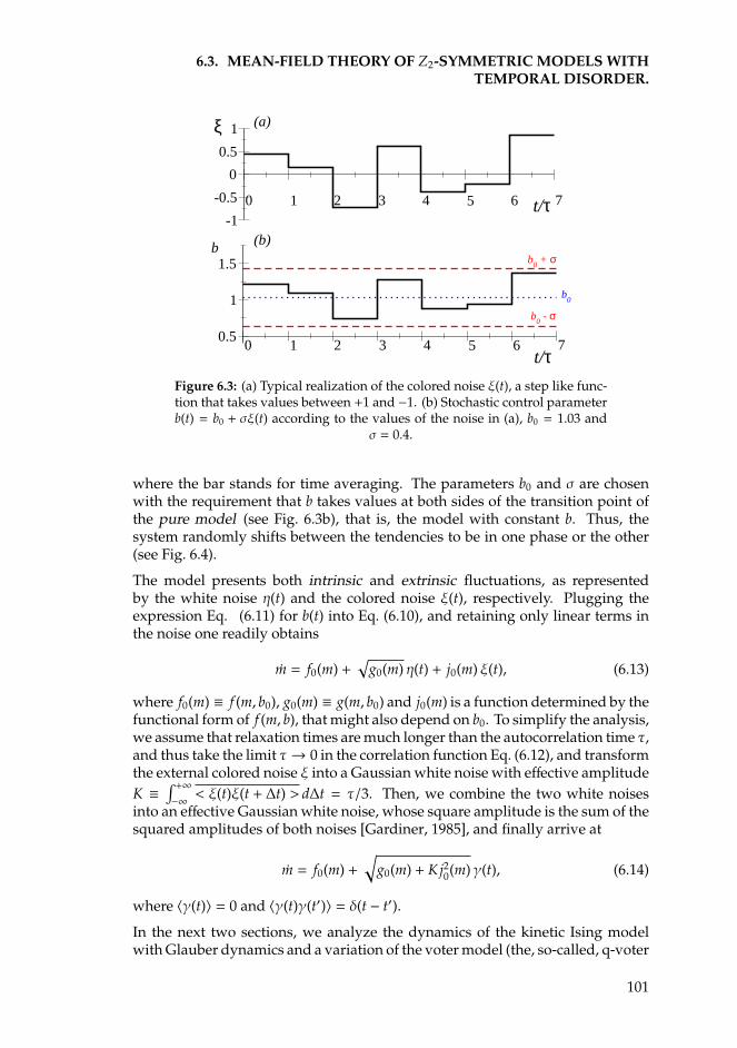
6.3. MEAN-FIELD THEORY OF Z2-SYMMETRIC MODELS WITHTEMPORAL DISORDER.
0 1 2 3 4 5 6 7t/τ-1
-0.5
0
0.5
1ξ
0 1 2 3 4 5 6 7t/τ
0.5
1
1.5b
b0 + σ
b0 - σ
(a)
(b)
b0
Figure 6.3: (a) Typical realization of the colored noise ξ(t), a step like func-tion that takes values between +1 and −1. (b) Stochastic control parameterb(t) = b0 + σξ(t) according to the values of the noise in (a), b0 = 1.03 and
σ = 0.4.
where the bar stands for time averaging. The parameters b0 and σ are chosenwith the requirement that b takes values at both sides of the transition point ofthe pure model (see Fig. 6.3b), that is, the model with constant b. Thus, thesystem randomly shifts between the tendencies to be in one phase or the other(see Fig. 6.4).
The model presents both intrinsic and extrinsic fluctuations, as representedby the white noise η(t) and the colored noise ξ(t), respectively. Plugging theexpression Eq. (6.11) for b(t) into Eq. (6.10), and retaining only linear terms inthe noise one readily obtains
m = f0(m) +√
g0(m) η(t) + j0(m) ξ(t), (6.13)
where f0(m) ≡ f (m, b0), g0(m) ≡ g(m, b0) and j0(m) is a function determined by thefunctional form of f (m, b), that might also depend on b0. To simplify the analysis,we assume that relaxation times are much longer than the autocorrelation time τ,and thus take the limit τ→ 0 in the correlation function Eq. (6.12), and transformthe external colored noise ξ into a Gaussian white noise with effective amplitudeK ≡
∫ +∞−∞ < ξ(t)ξ(t + ∆t) > d∆t = τ/3. Then, we combine the two white noises
into an effective Gaussian white noise, whose square amplitude is the sum of thesquared amplitudes of both noises [Gardiner, 1985], and finally arrive at
m = f0(m) +√
g0(m) + Kj20(m)γ(t), (6.14)
where 〈γ(t)〉 = 0 and 〈γ(t)γ(t′)〉 = δ(t − t′).
In the next two sections, we analyze the dynamics of the kinetic Ising modelwith Glauber dynamics and a variation of the voter model (the, so-called, q-voter
101
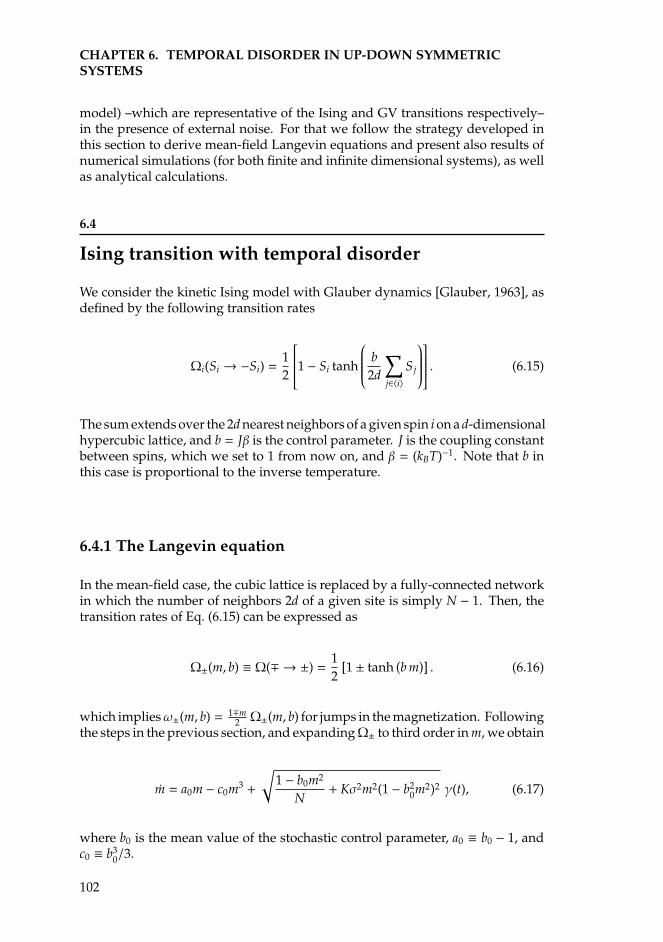
CHAPTER 6. TEMPORAL DISORDER IN UP-DOWN SYMMETRICSYSTEMS
model) –which are representative of the Ising and GV transitions respectively–in the presence of external noise. For that we follow the strategy developed inthis section to derive mean-field Langevin equations and present also results ofnumerical simulations (for both finite and infinite dimensional systems), as wellas analytical calculations.
6.4
Ising transition with temporal disorder
We consider the kinetic Ising model with Glauber dynamics [Glauber, 1963], asdefined by the following transition rates
Ωi(Si → −Si) =12
1 − Si tanh
b2d
∑j∈〈i〉
S j
. (6.15)
The sum extends over the 2d nearest neighbors of a given spin i on a d-dimensionalhypercubic lattice, and b = Jβ is the control parameter. J is the coupling constantbetween spins, which we set to 1 from now on, and β = (kBT)−1. Note that b inthis case is proportional to the inverse temperature.
6.4.1 The Langevin equation
In the mean-field case, the cubic lattice is replaced by a fully-connected networkin which the number of neighbors 2d of a given site is simply N − 1. Then, thetransition rates of Eq. (6.15) can be expressed as
Ω±(m, b) ≡ Ω(∓ → ±) =12
[1 ± tanh (b m)] . (6.16)
which impliesω±(m, b) = 1∓m2 Ω±(m, b) for jumps in the magnetization. Following
the steps in the previous section, and expandingΩ± to third order in m, we obtain
m = a0m − c0m3 +
√1 − b0m2
N+ Kσ2m2(1 − b2
0m2)2 γ(t), (6.17)
where b0 is the mean value of the stochastic control parameter, a0 ≡ b0 − 1, andc0 ≡ b3
0/3.
102
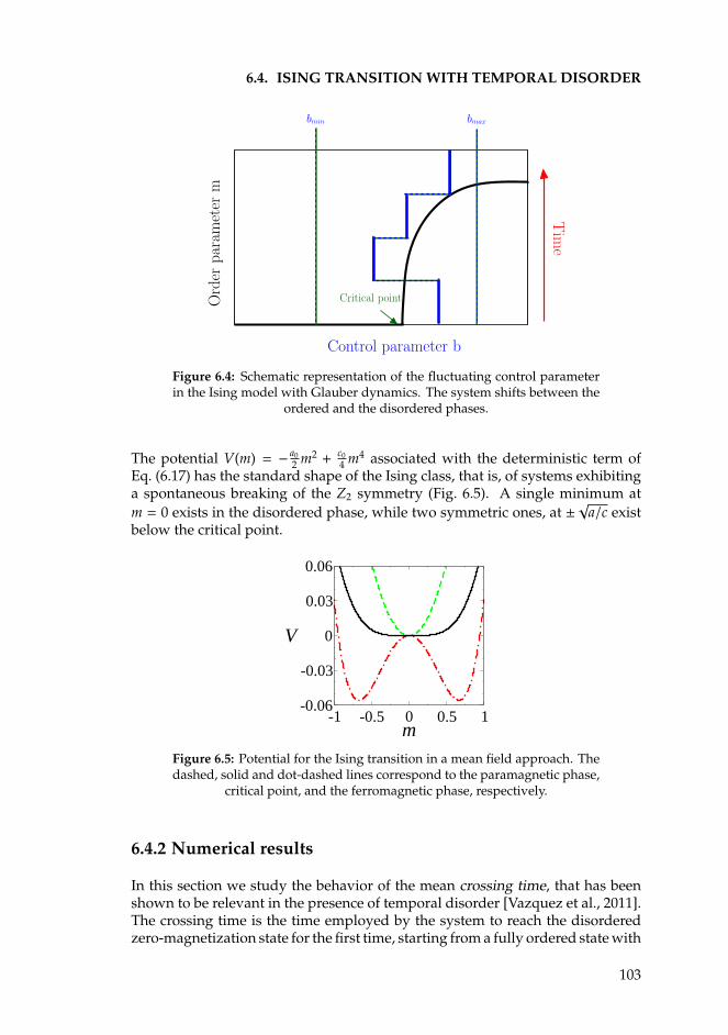
6.4. ISING TRANSITION WITH TEMPORAL DISORDER
Order
parameter
m
Control parameter b
Critical point
Tim
e
bmin bmax
Figure 6.4: Schematic representation of the fluctuating control parameterin the Ising model with Glauber dynamics. The system shifts between the
ordered and the disordered phases.
The potential V(m) = − a02 m2 + c0
4 m4 associated with the deterministic term ofEq. (6.17) has the standard shape of the Ising class, that is, of systems exhibitinga spontaneous breaking of the Z2 symmetry (Fig. 6.5). A single minimum atm = 0 exists in the disordered phase, while two symmetric ones, at ±
√a/c exist
below the critical point.
-1 -0.5 0 0.5 1m
-0.06
-0.03
0
0.03
0.06
V
Figure 6.5: Potential for the Ising transition in a mean field approach. Thedashed, solid and dot-dashed lines correspond to the paramagnetic phase,
critical point, and the ferromagnetic phase, respectively.
6.4.2 Numerical results
In this section we study the behavior of the mean crossing time, that has beenshown to be relevant in the presence of temporal disorder [Vazquez et al., 2011].The crossing time is the time employed by the system to reach the disorderedzero-magnetization state for the first time, starting from a fully ordered state with
103
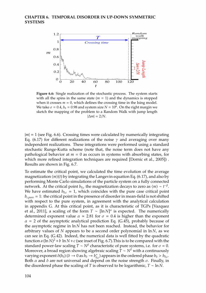
CHAPTER 6. TEMPORAL DISORDER IN UP-DOWN SYMMETRICSYSTEMS
t
m
0
0.2
0
TCrossing time
∆m=2/N
JumpLength
Randomwalk
mapping
0.4
0.6
0.8
1
1.2
20 40 60 80 120100
Figure 6.6: Single realization of the stochastic process. The system startswith all the spins in the same state (m = 1) and the dynamics is stoppedwhen it crosses m = 0, which defines the crossing time in the Ising model.We take σ = 0.4, b0 = 0.98 and system size N = 106. On the right margin wesketch the mapping of the problem to a Random Walk with jump length
|∆m| = 2/N.
|m| = 1 (see Fig. 6.6). Crossing times were calculated by numerically integratingEq. (6.17) for different realizations of the noise γ and averaging over manyindependent realizations. These integrations were performed using a standardstochastic Runge-Kutta scheme (note that, the noise term does not have anypathological behavior at m = 0 as occurs in systems with absorbing states, forwhich more refined integration techniques are required [Dornic et al., 2005]) .Results are shown in Fig. 6.7.
To estimate the critical point, we calculated the time evolution of the averagemagnetization 〈m〉(t) by integrating the Langevin equation Eq. (6.17), and also byperforming Monte Carlo simulations of the particle system on a fully connectednetwork. At the critical point b0,c the magnetization decays to zero as 〈m〉 ∼ t−β.We have estimated b0,c = 1, which coincides with the pure case critical pointbc,pure = 1: the critical point in the presence of disorder in mean-field is not shiftedwith respect to the pure system, in agreement with the analytical calculationin appendix G. At this critical point, as it is characteristic of TGPs [Vazquezet al., 2011], a scaling of the form T ∼ [ln N]α is expected. The numericallydetermined exponent value α ' 2.81 for σ = 0.4 is higher than the exponentα = 2 of the asymptotic analytical prediction Eq. (G.45), probably because ofthe asymptotic regime in ln N has not been reached. Instead, the behavior forarbitrary values of N appears to be a second order polynomial in ln N, as wecan see in Eq. (G.42). Indeed, the numerical data is well fitted by the quadraticfunction a (ln N)2+b ln N+c (see inset of Fig. 6.7).This is to be compared with thestandard power-law scaling T ∼ Nβ characteristic of pure systems, i.e. for σ = 0.Moreover, a broad region showing algebraic scaling T ∼ Nδ with a continuouslyvarying exponent δ(b0) (δ→ 0 as b0 → b+0,c) appears in the ordered phase b0 > b0,c.Both α and δ are not universal and depend on the noise strength σ. Finally, inthe disordered phase the scaling of T is observed to be logarithmic, T ∼ ln N.
104
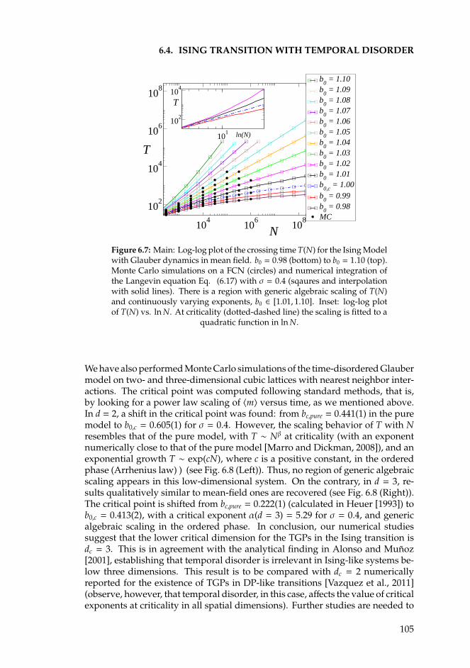
6.4. ISING TRANSITION WITH TEMPORAL DISORDER
104
106
108
N
102
104
106
108
T
b0 = 1.10
b0 = 1.09
b0 = 1.08
b0 = 1.07
b0 = 1.06
b0 = 1.05
b0 = 1.04
b0 = 1.03
b0 = 1.02
b0 = 1.01
b0,c
= 1.00b
0 = 0.99
b0 = 0.98
MC
101 ln(N)
102
104
T
Figure 6.7: Main: Log-log plot of the crossing time T(N) for the Ising Modelwith Glauber dynamics in mean field. b0 = 0.98 (bottom) to b0 = 1.10 (top).Monte Carlo simulations on a FCN (circles) and numerical integration ofthe Langevin equation Eq. (6.17) with σ = 0.4 (sqaures and interpolationwith solid lines). There is a region with generic algebraic scaling of T(N)and continuously varying exponents, b0 ∈ [1.01, 1.10]. Inset: log-log plotof T(N) vs. ln N. At criticality (dotted-dashed line) the scaling is fitted to a
quadratic function in ln N.
We have also performed Monte Carlo simulations of the time-disordered Glaubermodel on two- and three-dimensional cubic lattices with nearest neighbor inter-actions. The critical point was computed following standard methods, that is,by looking for a power law scaling of 〈m〉 versus time, as we mentioned above.In d = 2, a shift in the critical point was found: from bc,pure = 0.441(1) in the puremodel to b0,c = 0.605(1) for σ = 0.4. However, the scaling behavior of T with Nresembles that of the pure model, with T ∼ Nβ at criticality (with an exponentnumerically close to that of the pure model [Marro and Dickman, 2008]), and anexponential growth T ∼ exp(cN), where c is a positive constant, in the orderedphase (Arrhenius law) ) (see Fig. 6.8 (Left)). Thus, no region of generic algebraicscaling appears in this low-dimensional system. On the contrary, in d = 3, re-sults qualitatively similar to mean-field ones are recovered (see Fig. 6.8 (Right)).The critical point is shifted from bc,pure = 0.222(1) (calculated in Heuer [1993]) tob0,c = 0.413(2), with a critical exponent α(d = 3) = 5.29 for σ = 0.4, and genericalgebraic scaling in the ordered phase. In conclusion, our numerical studiessuggest that the lower critical dimension for the TGPs in the Ising transition isdc = 3. This is in agreement with the analytical finding in Alonso and Munoz[2001], establishing that temporal disorder is irrelevant in Ising-like systems be-low three dimensions. This result is to be compared with dc = 2 numericallyreported for the existence of TGPs in DP-like transitions [Vazquez et al., 2011](observe, however, that temporal disorder, in this case, affects the value of criticalexponents at criticality in all spatial dimensions). Further studies are needed to
105
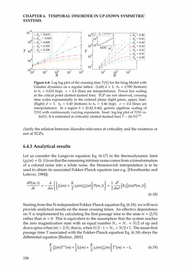
CHAPTER 6. TEMPORAL DISORDER IN UP-DOWN SYMMETRICSYSTEMS
102
103
104
105
106
N10
2
104
106
108
1010
T
b0 = 0.610
b0,c
= 0.605b
0 = 0.600
b0 = 0.595
b0 = 0.590
102
104
106
N
102
104
106
108
T
b0 = 0.46
b0 = 0.45
b0 = 0.44
b0 = 0.43
b0 = 0.42
b0 = 0.41
b0 = 0.40
101ln(N)
102
104
Tb
0 = 0.413
Figure 6.8: Log-log plot of the crossing time T(N) for the Ising Model withGlauber dynamics on a regular lattice. (Left) d = 2. b0 = 0.590 (bottom)to b0 = 0.610 (top). σ = 0.4 (lines are interpolations). Power law scalingat the critical point (dotted-dashed line). TGP are not observed, crossingtime scales exponentially in the ordered phase (light green, upper, line).(Right) d = 3. b0 = 0.40 (bottom) to b0 = 0.46 (top). σ = 0.4 (lines areinterpolations). In a region b ∈ [0.42, 0.46], generic algebraic scaling ofT(N) with continuously varying exponents. Inset: log-log plot of T(N) vs.
ln(N). It is estimated at criticality (dotted-dashed line) T ∼ (ln N)5.29.
clarify the relation between disorder-relevance at criticality and the existence ornot of TGPs.
6.4.3 Analytical results
Let us consider the Langevin equation Eq. (6.17) in the thermodynamic limit(g0(m) = 0). Given that the remaining intrinsic noise comes from a transformationof a colored noise into a white noise, the Stratonovich interpretation is to beused to obtain its associated Fokker-Planck equation (see e.g. [Horsthemke andLefever, 1984])
∂P(m, t)∂t
= − ∂∂m
[f0(m) +
K2
j0(m) j′0(m)]
P(m, t)+
12∂2
∂m2
Kj20(m)P(m, t)
.
(6.18)
Starting from this N-independent Fokker-Planck equation Eq. (6.18), we will nextprovide analytical results on the mean crossing times. An effective dependenceon N is implemented by calculating the first-passage time to the state m = |2/N|rather than m = 0. This is equivalent to the assumption that the system reachesthe zero magnetization state with an equal number N+ = N− = N/2 of up anddown spins when |m| < 2/N, that is, when N/2−1 < N+ < N/2+1. The mean-firstpassage time T associated with the Fokker-Planck equation Eq. (6.18) obeys thedifferential equation [Redner, 2001]
K2
j20(m)T′′(m) +[
f0(m) +K2
j0(m) j′0(m)]
T′(m) = −1, (6.19)
106
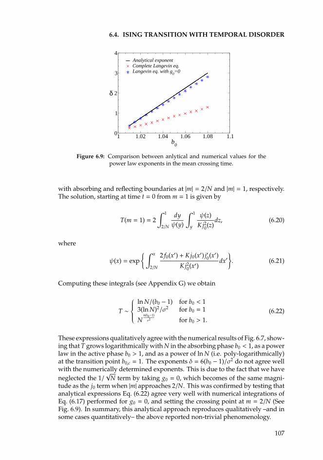
6.4. ISING TRANSITION WITH TEMPORAL DISORDER
1 1.02 1.04 1.06 1.08 1.1b
0
0
1
2
3
4
δ
Analytical exponentComplete Langevin eq.Langevin eq. with g
0=0
Figure 6.9: Comparison between anlytical and numerical values for thepower law exponents in the mean crossing time.
with absorbing and reflecting boundaries at |m| = 2/N and |m| = 1, respectively.The solution, starting at time t = 0 from m = 1 is given by
T(m = 1) = 2∫ 1
2/N
dyψ(y)
∫ 1
y
ψ(z)
Kj20(z)dz, (6.20)
where
ψ(x) = exp∫ x
2/N
2 f0(x′) + Kj0(x′) j′0(x′)
Kj20(x′)dx′
. (6.21)
Computing these integrals (see Appendix G) we obtain
T ∼
ln N/(b0 − 1) for b0 < 13(ln N)2/σ2 for b0 = 1
N6(b0−1)
σ2 for b0 > 1.(6.22)
These expressions qualitatively agree with the numerical results of Fig. 6.7, show-ing that T grows logarithmically with N in the absorbing phase b0 < 1, as a powerlaw in the active phase b0 > 1, and as a power of ln N (i.e. poly-logarithmically)at the transition point b0,c = 1. The exponents δ = 6(b0 − 1)/σ2 do not agree wellwith the numerically determined exponents. This is due to the fact that we haveneglected the 1/
√N term by taking g0 = 0, which becomes of the same magni-
tude as the j0 term when |m| approaches 2/N. This was confirmed by testing thatanalytical expressions Eq. (6.22) agree very well with numerical integrations ofEq. (6.17) performed for g0 = 0, and setting the crossing point at m = 2/N (SeeFig. 6.9). In summary, this analytical approach reproduces qualitatively –and insome cases quantitatively– the above reported non-trivial phenomenology.
107
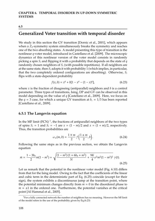
CHAPTER 6. TEMPORAL DISORDER IN UP-DOWN SYMMETRICSYSTEMS
6.5
Generalized Voter transition with temporal disorder
We study in this section the GV transition [Dornic et al., 2001], which appearswhen a Z2-symmetry system simultaneously breaks the symmetry and reachesone of the two absorbing states. A model presenting this type of transition is thenonlinear q-voter model, introduced in Castellano et al. [2009]. The microscopicdynamics of this nonlinear version of the voter model consists in randomlypicking a spin Si and flipping it with a probability that depends on the state of qrandomly chosen neighbors of Si (with possible repetitions). If all neighbors areat the same state, then Si adopts it with probability 1 (which implies, in particular,that the two completely ordered configurations are absorbing). Otherwise, Siflips with a state-dependent probability
f (x, b) = xq + b[1 − xq − (1 − x)q], (6.23)
where x is the fraction of disagreeing (antiparallel) neighbors and b is a controlparameter. Three types of transitions, Ising, DP and GV can be observed in thismodel depending on the value of q [Castellano et al., 2009]. Here, we focus onthe q = 3 case, for which a unique GV transition at bc = 1/3 has been reported[Castellano et al., 2009].
6.5.1 The Langevin equation
In the MF limit (FCN) 1, the fractions of antiparallel neighbors of the two typesof spins Si = 1 and Si = −1 are x = (1 − m)/2 and x = (1 + m)/2, respectively.Thus, the transition probabilities are
ω±(m, b) =1 ∓m
2f(1 ±m
2, b
). (6.24)
Following the same steps as in the previous section, we obtain the Langevinequation
m =1 − 3b0
2m(1 −m2) +
√(1 −m2) (1 + 6b0 +m2)
N+
9K4σ2m2(1 −m2)2 γ(t).
(6.25)
Let us remark that the potential in the nonlinear voter model (Fig. 6.10) differsfrom that for the Ising model. Owing to the fact that the coefficients of the linearand cubic term in the deterministic part of Eq. (6.25) coincide (except for theirsign), the system exhibits a discontinuous jump at the transition point, wherethe potential minimum changes directly from m = 0 in the disordered phase tom = ±1 in the ordered one. Furthermore, the potential vanishes at the criticalpoint [Al Hammal et al., 2005].
1For a fully connected network the number of neighbors has no meaning. However the Mf limitof the model refers to the use of the probability given by Eq.(6.23)
108
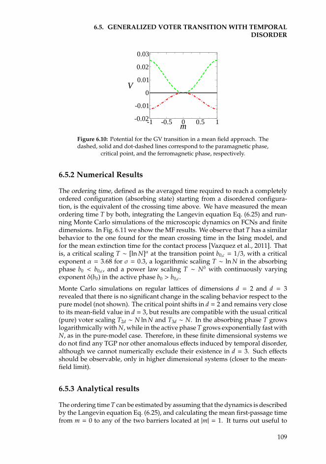
6.5. GENERALIZED VOTER TRANSITION WITH TEMPORALDISORDER
-1 -0.5 0 0.5 1m
-0.02
-0.01
0
0.01
0.02
0.03
V
Figure 6.10: Potential for the GV transition in a mean field approach. Thedashed, solid and dot-dashed lines correspond to the paramagnetic phase,
critical point, and the ferromagnetic phase, respectively.
6.5.2 Numerical Results
The ordering time, defined as the averaged time required to reach a completelyordered configuration (absorbing state) starting from a disordered configura-tion, is the equivalent of the crossing time above. We have measured the meanordering time T by both, integrating the Langevin equation Eq. (6.25) and run-ning Monte Carlo simulations of the microscopic dynamics on FCNs and finitedimensions. In Fig. 6.11 we show the MF results. We observe that T has a similarbehavior to the one found for the mean crossing time in the Ising model, andfor the mean extinction time for the contact process [Vazquez et al., 2011]. Thatis, a critical scaling T ∼ [ln N]α at the transition point b0,c = 1/3, with a criticalexponent α = 3.68 for σ = 0.3, a logarithmic scaling T ∼ ln N in the absorbingphase b0 < b0,c, and a power law scaling T ∼ Nδ with continuously varyingexponent δ(b0) in the active phase b0 > b0,c.
Monte Carlo simulations on regular lattices of dimensions d = 2 and d = 3revealed that there is no significant change in the scaling behavior respect to thepure model (not shown). The critical point shifts in d = 2 and remains very closeto its mean-field value in d = 3, but results are compatible with the usual critical(pure) voter scaling T2d ∼ N ln N and T3d ∼ N. In the absorbing phase T growslogarithmically with N, while in the active phase T grows exponentially fast withN, as in the pure-model case. Therefore, in these finite dimensional systems wedo not find any TGP nor other anomalous effects induced by temporal disorder,although we cannot numerically exclude their existence in d = 3. Such effectsshould be observable, only in higher dimensional systems (closer to the mean-field limit).
6.5.3 Analytical results
The ordering time T can be estimated by assuming that the dynamics is describedby the Langevin equation Eq. (6.25), and calculating the mean first-passage timefrom m = 0 to any of the two barriers located at |m| = 1. It turns out useful to
109
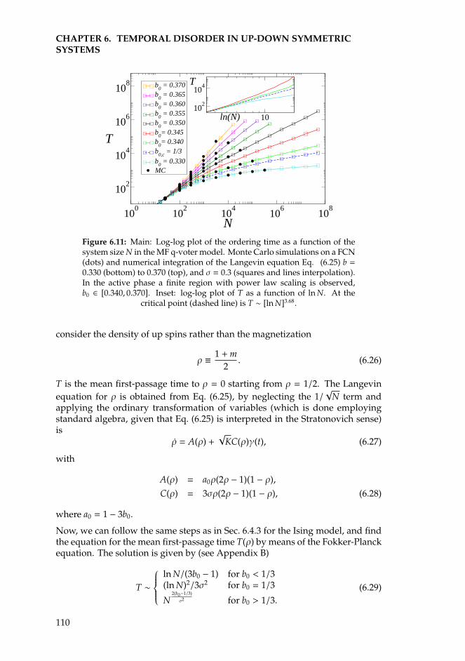
CHAPTER 6. TEMPORAL DISORDER IN UP-DOWN SYMMETRICSYSTEMS
100
102
104
106
108
N
102
104
106
108
T
b0 = 0.370
b0 = 0.365
b0 = 0.360
b0 = 0.355
b0 = 0.350
b0= 0.345
b0= 0.340
b0,c
= 1/3
b0 = 0.330
MC
10ln(N)10
2
104T
Figure 6.11: Main: Log-log plot of the ordering time as a function of thesystem size N in the MF q-voter model. Monte Carlo simulations on a FCN(dots) and numerical integration of the Langevin equation Eq. (6.25) b =0.330 (bottom) to 0.370 (top), and σ = 0.3 (squares and lines interpolation).In the active phase a finite region with power law scaling is observed,b0 ∈ [0.340, 0.370]. Inset: log-log plot of T as a function of ln N. At the
critical point (dashed line) is T ∼ [ln N]3.68.
consider the density of up spins rather than the magnetization
ρ ≡ 1 +m2
. (6.26)
T is the mean first-passage time to ρ = 0 starting from ρ = 1/2. The Langevinequation for ρ is obtained from Eq. (6.25), by neglecting the 1/
√N term and
applying the ordinary transformation of variables (which is done employingstandard algebra, given that Eq. (6.25) is interpreted in the Stratonovich sense)is
ρ = A(ρ) +√
KC(ρ)γ(t), (6.27)
with
A(ρ) = a0ρ(2ρ − 1)(1 − ρ),C(ρ) = 3σρ(2ρ − 1)(1 − ρ), (6.28)
where a0 = 1 − 3b0.
Now, we can follow the same steps as in Sec. 6.4.3 for the Ising model, and findthe equation for the mean first-passage time T(ρ) by means of the Fokker-Planckequation. The solution is given by (see Appendix B)
T ∼
ln N/(3b0 − 1) for b0 < 1/3(ln N)2/3σ2 for b0 = 1/3
N2(b0−1/3)
σ2 for b0 > 1/3.(6.29)
110
6.6. SUMMARY AND CONCLUSIONS
These scalings, which qualitatively agree with the numerical results of Fig. 6.11for the q-voter, show that the behavior of T is analogous to the one observed inthe Ising transition of section 6.4 and in the DP transition found in Vazquez et al.[2011]. Therefore, we conclude that TGPs appear around GV transitions in thepresence of external varying parameters in high dimensional systems.
For the GV universality class the renormalization group fixed point is a non-perturbative one [Canet et al., 2005], becoming relevant in a dimension betweenone and two. A field theoretical implementation of temporal disorder in this the-ory is still missing, hence, theoretical predictions and sound criteria for disorderrelevance are not available.
6.6
Summary and conclusions
We have investigated the effect of temporal disorder on phase transitions exhib-ited by Z2 symmetric systems: the (continuous) Ising and (discontinuous) GVtransitions which appear in many different scenarios. We have explored whethertemporal disorder induces Temporal Griffiths Phases as it was previously foundin standard (DP) systems with one absorbing state. By performing mean-fieldanalyses as well as extensive computer simulations (in both fully connected net-works and in finite dimensional lattices) we found that TGPs can exist aroundequilibrium (Ising) transitions (above d = 2) and around discontinuous (GV)non-equilibrium transitions (only in high-dimensional systems).
Therefore, we confirm that TGPs may also appear in systems with two sym-metric absorbing states, illustrating the generality of the underlying mechanism:the appearance of a region, induced by temporal stochasticity of the control pa-rameter, where first-passage times scale as power laws of the system size. Thealgebraic scaling of the crossing time, compared with the exponential one ob-served in pure system, shows that temporal disorder makes the ordered/activephase less stable. This implies that the system becomes highly susceptible toperturbations. This appears to be a rather general and robust phenomenon andan relevant result with applications in ecology. As it has been said before, the ex-tinction times that have been quantified in this chapter can be identified, in somecases, with population lifetimes. Considering the effect of the environmentalvariability, habitat fragmentation becomes a more important threat when sys-tems become larger, where the exponential behavior scales much faster than thealgebraic one.
Additionally, although it is of secondary interest to our focus on ecological sys-tems and it has been not shown in this chapter, we have also confirmed that theresponse function of the system (i.e. susceptibility) diverges in a finite regionclose to the critical point. This complementary result has been also obtained inVazquez et al. [2011] and confirms the phenomelogical similarities between Tem-poral Griffiths Phases and Griffiths Phases in systems with quenched disorder.
111
CHAPTER 6. TEMPORAL DISORDER IN UP-DOWN SYMMETRICSYSTEMS
It also seems to be a general property that TGPs do not appear in low dimensionalsystems, where standard fluctuations dominate over temporal disorder. In allthe cases studied so far, a critical dimension dc –at and below which TGPs do notappear– exist (dc = 1 for DP transitions, dc = 2 for Ising like systems, and dc ' 3for GV ones). Calculating analytically such a critical dimension and comparingit with the standard critical dimension for the relevance/irrelevance of temporaldisorder at the critical point (i.e. at the renormalization group non-trivial fixedpoint of the corresponding field theory) remains an open and challenging task.
Future research might be oriented to the effect of temporal disorder on theformation and dynamics of spatial structures.
112
APPENDIX FIto-Stratonovich discussion.
The integration of stochastic differential equations with multiplicative whitenoise presents some problems because the integral of the noise is not well defined.These problems are solved choosing either the Ito or the Stratonovich definitionof the integral.1
We have chosen one or the other depending on the origin of the noise term inthe Langevin equation. This Appendix explains how Ito’s calculus works, andthe connection between Ito and Stratonovich schemes. We will finish discussingin what of them is more suitable in each situation.
F.1
Stochastic integration.
Let us start providing a precise definition of the second integral in
M(t) −M(0) =∫ t
0f [M(s), s]ds +
∫ t
0g[M(s), s]dW(s), (F.1)
that is ∫ t
0G(s)dW(s). (F.2)
The integration interval [0, t] is divided into n subintervals,
0 ≤ t1 ≤ t2 ≤ t3... ≤ tn−1 ≤ tn, (F.3)
and the intermediate points in each interval τi defined
τi = ti−1 + α(ti − ti−1). (F.4)
1Any definition can be chosen or even made, but these two are the most often used.
113
APPENDIX F. ITO-STRATONOVICH DISCUSSION.
The stochastic integral in Eq. (F.2) is defined as the limit of the partial sums,
Sn =
n∑i=1
G(τi)(W(ti) −W(ti−1)), (F.5)
where the Ito vs Stratonovich dilemma resides in the fact that the limit of Sndepends on the particular set of points τi that are used. Ito stochastic integral isdefined taking α = 0, so Eq. (F.5) becomes
Sn =
n∑i=1
G(ti−1)(W(ti) −W(ti−1)), (F.6)
that is, the known function g(x(t)) is evaluted on the beginning point of theinterval while Stratonovich is obtained if α = 1/2 and
Sn =
n∑i=1
G( ti−1 + ti
2
)(W(ti) −W(ti−1)). (F.7)
F.2
Ito’s formula.
In spite of being much more elegant from a mathematical point of view, Ito’sprescription is not always the most suitable choice for physical interpretation.Calculus we are used to does not work in this scheme and a different changeof variables must be considered. To begin with, lets take an arbitrary functiona[x(t)] with x(t) obeying the SDE
dx(t)dt= f (x, t) + g(x, t)ξ(x, t), (F.8)
where ξ(x, t) is a white Gaussian noise. Consider
da[x(t)] = a[x(t) + dx(t)] − a[x(t)]
= a′[x(t)]dx(t) +12
a′′[x(t)]dx2(t) + ...
= a′[x(t)]f (x, t) + g(x, t)ξ(t)
dt +
12
a′′[x(t)]g2(x, t)dW2(t) + ...,
(F.9)
where higher terms in dt have been neglected. Now, replacing dW2(t) = dt (see[Gardiner, 1985] for a proof),
da[x(t)] = a′[x(t)]
f (x, t) +12
a′′[x(t)]g2(x, t)
dt + a′′[x(t)]g(x, t)dW(t), (F.10)
which is known as the Ito’s formula and shows that change of variables is notgiven by ordinary calculus unless a[x(t)] is linear in x(t).
114
F.3. FROM STRATONOVICH TO ITO.
F.3
From Stratonovich to Ito.
As may be expected, both interpretations of the stochastic integral are somehowrelated. To show it, consider an stochastic differential equation
dxdt= α[x(t), t] + β[x(t), t]η(t), (F.11)
where η(t) is a white, zero mean, Gaussian noise. Integrating, it is,
x(t) = x(0) +∫ t
0α[x(s), s]ds + S
∫ t
0β[x(s), s]dW(s), (F.12)
where S denotes that a Stratonovich integration is used. We will derive theequivalent Ito stochastic differential equation.
Assuming that x(t) is a solution of
dx(t) = a[x(t), t]dt + b[x(t), t]dW(t), (F.13)
the corresponding α[x(t), t] and β[x(t), t] will be deduced. The first step is tocompute the connection between S
∫ t
0 β[x(s), s]dW(s) and∫ t
0 β[x(s), s]dW(s), wherethe lack of notation in the second integral means an Ito interpretation. Then,
S∫ t
0β[x(s), s]dW(s) ≈
∑i
β
[x(ti) + x(ti−1)
2, ti−1
][W(ti) −W(ti−1)] . (F.14)
Taking into an accountx(ti) = x(ti−1) + dx(ti−1), (F.15)
in the Stratonovich integral, then
β
[x(ti) + x(ti−1)
2, ti−1
]= β
[x(ti−1) +
12
dx(ti−1), ti−1
]. (F.16)
Now, the Ito SDE (F.13) is used in order to write
dx(ti) = a[x(ti−1), ti−1](ti − ti−1) + b[x(ti−1), ti−1][W(ti) −W(ti−1)]. (F.17)
Using Ito’s formula given by Eq. (F.10) as well as simplifying the notation writingβ(ti−1) instead of β[x(ti−1), ti−1], Eq. (F.16) becomes,
β
[x(ti) + x(ti−1)
2, ti−1
]= β(ti−1) +
[a(ti−1)∂xβ(ti−1) +
14
b2(ti−1)] [1
2(ti − ti−1)
]+
+12
b(ti−1)∂xβ(ti−1)[W(ti) −W(ti−1)]. (F.18)
115
APPENDIX F. ITO-STRATONOVICH DISCUSSION.
Finally, substituing into Eq. (F.14), neglecting terms in dt2 and dWdt and settingdW2 = dt,
S∫=
∑i
β(ti−1)(W(ti) −W(ti−1)) +12
∑i
b(ti−1)∂xβ(ti−1)(ti − ti−1), (F.19)
or going back to integrals,
S∫ t
0β[x(s), s]dW(s) =
∫ t
0β[x(s), s]dW(s) +
12
∫ t
0b[x(s), s]∂xβ[x(s), s]ds, (F.20)
which means that the stochastic integral in Stratonovich representation is equiv-alent to a stochastic integral in Ito’s and a drift term. It is also important to remarkthat this formula gives a connection between both integrals of function β[x(s), s],in which x(s) is the solution of the Ito SDE (F.13). It does not give a generalconnection between the Ito and Stratonovich integrals of arbitrary functions.
The Ito SDE dx = a(x, t)dt + b(x, t)dW(t)
is the Stratonovich SDE dx =[a(x, t) − 1
2b(x, t)∂xb(x, t)
]dt + b(x, t)dW(t).
(F.21)
Or
The Stratonovich SDE dx = αdt + βdW(t)
is the Ito SDE dx =[α(x, t) +
12β(x, t)∂xβ(x, t)
]dt + β(x, t)dW(t).
(F.22)
There are many consequences of this transformation formula, but the moreimportant are
• It is always possible to change from the Stratonovich to the Ito interpreta-tion of a SDE by adding 1
2β(x, t)∂xβ(x, t) or in the inverse direction subtract-ing a similar term.
• In the case of additive noise, i.e., g(x, t) = const. in Eq. (F.8) there is nodifference between the Ito and Stratonovich integral.
• In the case of multiplicative noise, i.e., g(x, t) , const. in Eq. (F.8), wherethe influence of the random force depends on the state of the process, thecorrelation between both the random force and the state of the process isimplicit in the Stratonovich integral. It gives raise to the noise induced driftwhen moving to Ito appearing in the deterministic part of the equation.
• The Stratonovich calculus obeys the classical chain rule, Ito’s formula de-rived in Section F.2 plays a similar role on Ito’s calculus.
116
F.4. STRATONOVICH / ITO DILEMMA.
F.4
Stratonovich / Ito dilemma.
The long controversy in the physical literature about what is the right definitionof the stochastic integral has created some confusion on this topic. That’s why,although a much more mathematically rigorous and longer discussion can befound in the references, [van Kampen, 2007; Horsthemke and Lefever, 1984;Jazwinski, 2007] some hand waving arguments will be given in this section.
First of all it is important to say that this kind of ambiguity when workingwith SDE only yields for the particular, but most common, case of differentialequations with multiplicative white noise2. As a first approach, it is naturalto tend to believe that due to invariance of the equations under “coordinatetransformation” y = u(x) when working on Stratonovich scheme it is the properchoice. However, it means nothing but it obeys the classical calculus ruleswe are familiar with. The only quantities that have to be invariant under atransformation u = y(x), where u is one to one, are the probabilities,
p(y, t)dy = p(x, t)dx, (F.23)
and this is of course guaranteed in both calculi. They lead to a consistent calculus.
It looks sensible, then, to change the question. The matter is not what is theright definition of the stochastic integral, but how do we model real systemsby stochastic processes. That is, in which situation either Ito’s or Stratonovich’schoice is the most suitable.
On the one hand, if the starting point is a phenomenological equation in whichsome fluctuating parameters represented through colored noise terms are ap-proximated by Gaussian white noise, then the most appropiate process is theone that is defined by the Stratonovich interpretation of the equation.
On the other hand, in many systems the appropiate starting point is a discret timeequation, as it happens, for instance, in biology when working with populationsof insects. In these cases the equation reads
X(ti) = X(ti−1) + f (X(ti−1))∆t + σg(X(ti−1))Q(ti−1), (F.24)
where ti = ti−1 +∆t in every time step and Qi are Gaussian independent randomvariables with expected values < Q(ti) >= 0 and < Q2(ti) >= ∆t.
If times considered are longer compared to ∆t, the continuous time limit can betaken. Then the system is described by
X(t) = f [X(t)] + σg[X(t)]W(t), (F.25)
which is also a SDE where W(t) is the Wiener process. However, due to theasymmetric form of Eq. (F.24) with respect to time it is much more appropiatethe stochastic process defined according to the Ito interpretation in this case.
2Cases where the rapidly fluctuating external force depends on the state of the system.
117

APPENDIX F. ITO-STRATONOVICH DISCUSSION.
To sum up, as a take to home message from this section, two different cases canbe considered when working with SDE. When the white Gaussian noise limit isconsidered as the limit of a colored noise when the correlation time tends to zero,the Stratonovich interpretation is more sensible, when Ito’s is more suitable whenit represents the continuous limit of a discrete time problem. In any case, thereare no universally valid theoretical reasons why one or the other interpretationof an SDE should be preferred and the ultimate test must be the confrontation ofthe analytical (or numerical) results with the experimental facts.
118
APPENDIX GAnalytical calculations on the
escape time for the Ising Model
We will show here all the analytical calculations done to obtain the result ofEq. (6.22). To make the integrals analytically solvable we take g1,0(m) = 0, so theLangevin equation is
m = f0(m) +√
Kj0(m)γ(t), (G.1)
with
f0(m) = a0m − c0m3,
j0(m) = σm(1 − b20m2), (G.2)
where a0 = b0 − 1, c0 = b30/3 and γ(t) is, again, a white Gaussian noise defined by
its autocorrelation function< γ(t)γ(t′) >= δ(t−t′), and its mean value< γ(t) >= 0.
The Langevin equation (G.1) presents one absorbing state in m = 0 induced bythe simplification done when neglecting thermal fluctuations.
Working in the Stratonovich scheme 1, the associated Fokker-Planck equation is
∂P(m, t)∂t
= − ∂∂m
[f0(m) +
K2
j0(m) j′0(m)]
P(m, t) +K2∂2
∂m2
[j20(m)P(m, t)
],
(G.3)
where
f0(m) +K2
j0(m) j′0(m) =(a0 +
τ6σ2
)m +
τσ2
2b4
0m5 −c0 +
2τσ2b20
3
m3,
Dj20(m) =τ3σ2m2
(1 − b2
0m2)2. (G.4)
According to Gardiner [1985] and Redner [2001], the escape time from an startingpoint m obeys, [
f0(m) +K2
j0(m) j′0(m)]
T′(m) +12
Kj20(m)T′′(m) = −1. (G.5)
1Because the noise term comes from taking the white noise limit in a colored one
119
APPENDIX G. ANALYTICAL CALCULATIONS ON THE ESCAPE TIMEFOR THE ISING MODEL
As the size of the system does not appear naturally in the problem because of thesimplification done when taking g1,0 = 0, the mean escape time will be definedas that needed to pass through m = 2/N, which is the length of the jumps of theBrownian particle to whose movement the problem has been mapped. Then,taking into an account that there is an absorbing barrier in m = 0 and a reflectingone in m = 1 and the initial condition, the solution is [Gardiner, 1985]
T(mi = 1) = 2∫ mi=1
2/N
dyψ(y)
∫ 1
y
ψ(z)
Kj20(z)dz, (G.6)
with
ψ(z) = exp∫ z
2/Ndz′
2 f (z′) + Kj0(z′) j′0(z′)
Kj20(z′), (G.7)
which involves 6th and 4th order polynomial functions.
To make the integral simpler, we expand the functions up to 3rd order, and takrethe low integration limit in Eq. (G.7) at 1 instead of 2/N. This change can be donebecause ψ(z) appears both in the numerator and the denominator of T(m), so thecontribution of the lower limit vanishes, allowing to take it in our interest. Thefirst assumption leads to
f0(m) +K2
j0(m) j′0(m) ≈ m(r − sm2),
Kj20(m) ≈ ωm2, (G.8)
where it has been defined ω ≡ τσ2/3; r ≡ a0 +ω/2; s ≡ (c0 + 2ωb20). The size of the
system will be rescaled too, so the lower limit in the expression of the escape timeEq. (G.6) is 1/N. This simplifies the notation and does not affect the qualitativebehaviour of the results in the asymptotic limit (only a constant factor appears).
Now, it can be written,
ψ(z) = exp∫ z
1
2z′(r − sz′2)ωz′2
dz′ = zαeβ(1−z2), (G.9)
where α ≡ 2r/ω and β ≡ s/ω.
Lets now define the function
I(y) =∫ 1
y
ψ(z)
Kj20(z)dz =
eβ
ω
∫ 1
yzα−2e−βz2
dz, (G.10)
which presents a singularity when α = 1 as can be seen integrating by parts.With the definition made of the parameters, it can be shown that it correspondsto b0 = 1 ≡ b0,c.
120
G.1. CASE α , 1
Considering the definitions of Eq. (G.9) and Eq. (G.10), the mean escape time isgiven by
T = 2∫ 1
1/N
I(y)ψ(y)
dy. (G.11)
Each case will be studied separately.
G.1
Case α , 1
Integrating by parts Eq. (G.10)
I(y) =eβ
ω
e−β − e−βy2 yα−1
α − 1+ 2β
∫ 1
y
zαe−βz2
α − 1dz
, (G.12)
where the new integral can be solved again integrating by parts. Workingrecursively this way,
I(y) =eβ
ω
e−β − e−βy2 yα−1
α − 1+ 2β
e−β − e−βy2 yα+1
(α − 1)(α + 1)+ ...
, (G.13)
or
I(y) =1ω
∞∑k=0
(2β)k 1 − e−β(y2−1)yα−1+2k∏ki=0(α − 1 + 2i)
. (G.14)
The mean escape time is given now by
T =2ω
∞∑k=0
(2β)k∏ki=0(α − 1 + 2i
[I1(N) − I2(k,N)] , (G.15)
where
I1(N) ≡∫ 1
1/Ny−αeβ(y2−1)dy (G.16)
I2(k,N) ≡∫ 1
1/Ny2k−1dy. (G.17)
Integrating I1(N) by parts (taking again the exponential part as u and the rest asdv) and following the same procedure as in Eq. (G.10) it is obtained
I1(N) =∞∑
l=0
(−2β)l[1 −Nα−1−2leβ(1/N2−1)]∏lj=0(α − 1 + 2 j)
, (G.18)
while I2(k,N) is easily solved
I2(k,N) =−ln(N−1) = ln(N) for k = 0,1−N−2k
2k for k ≥ 1.(G.19)
121

APPENDIX G. ANALYTICAL CALCULATIONS ON THE ESCAPE TIMEFOR THE ISING MODEL
At the end, an expresion for the mean escape time is achieved
T =2ω
(I1(N) − ln(N)
α − 1
)
+2ω
∞∑k=1
(2β)k[I1(N) − (1 −N−2k)/2k
]∏k
i=0(α − 1 + 2i).
(G.20)
In the asymptotic limit N→∞ two different cases must be considered.
G.1.1 α < 1
Under this prescription, α − 1 − 2l < 0 when l ≥ 0 so in I1(N)
1 −Nα−1−2leβ(1/N2−1) ∼ 1 − e−β
Nν∼ 1, (G.21)
which leads to
I1(N) =∞∑
l=0
(−2β)l∏lj=0(1 + 2 j − α
≡ C(α, β). (G.22)
Finally, for the mean escape time,
T ≈ 2ω
C(α, β) − ln(N)α − 1
+
∞∑k=1
(2β)k(C(α, β) − (2k)−1
)∏l
j=0(α − 1 + 2 j)
, (G.23)
what means,
T ≈ 2ω(α − 1)
ln(N). (G.24)
G.1.2 α > 1
It is taken as a starting point
I1(N) =∞∑
l=0
(−2β)l[1 −Nα−1−2leβ(1/N2−1)]∏lj=0(α − 1 + 2 j)
, (G.25)
where considering that Nα−1 Nα−1−2l,∀l > 0, only the first term in Eq. (G.25) isrelevant. It implies
I1(N) ≈ 1 − e−βNα−1
1 − α ≈ e−βNα−1
1 − α , (G.26)
and in the mean escape time
T ≈ K(α, β)Nα−1 − 2ln(N)ω(α − 1)
∼ Nα−1 (N 1).
(G.27)
122
G.2. CASE α = 1 CRITICAL POINT.
G.2
Case α = 1 Critical point.
It has to be solved now
I(y) =∫ 1
y
ψ(z)
Kj20(z)dz =
eβ
ω
∫ 1
yy−1e−βz2
dz, (G.28)
using the expansion of the exponential function and integrating it is
I(y) =eβ
ω
−ln(y) +∞∑
k=1
(−β)k(1 − 2y)2k
k!2k
. (G.29)
It makes the mean escape time to obey, taking the form of I(y) Eq. (G.29) intoEq. (G.11)
T =2eβ
ω
I3(N) +∞∑
k=1
(−β)k
k!2k(I4(N) + I5(k,N))
, (G.30)
where
I3(N) = −∫ 1
1/Nln(y)y−1eβ(y2−1)dy,
I4(N) =
∫ 1
1/Ny−1eβ(y2−1)dy,
I5(k,N) =
∫ 1
1/Nyk−1eβ(y2−1)dy. (G.31)
First of all, lets consider the solution of I3(N) integrating by parts (u = eβy2and
dv = ln(y)y−1dy) so,
I3(N) =(lnN)2
2eβ(N−2−1) + β
∫ 1
1/N(lny)2eβ(y2−1)dy, (G.32)
where the new integral is solved again integrating by parts taking
u = eβ(y2−1) → du = 2βeβ(y2−1)
dv = (lny)2dy→ v = 2y − 2ylny + y(lny)2.
(G.33)
It leads to a solution behaving like
β
∫ 1
1/N(lny)2eβ(y2−1)dy = 2β −O(N−1) +O
( lnNN
), (G.34)
123
APPENDIX G. ANALYTICAL CALCULATIONS ON THE ESCAPE TIMEFOR THE ISING MODEL
so finally,
I3(N) =(lnN)2
2eβ(N−2−1) + 2β −O(N−1) +O
( lnNN
), (G.35)
which scales in the asymptotic limit as
I3(N) ∼ (lnN)2
2e−β. (G.36)
Secondly, lets focus on I4(N), where, again, an expansion of the exponentialfunction has to be done
I4(N) =∫ 1
1/Ny−1eβ(y2−1)dy = e−β
∫ 1
1/Ny−1
∞∑k=0
βk y2k
k!dy (G.37)
which can be easily solved
I4(N) = e−β[lnN +
βk
k!2k
(1 −N−2k
)]. (G.38)
The leading behavior when the size of the system is big enough (N 1) is
I4(N) ∼ e−βlnN + C4(β). (G.39)
The last integral to be solved, also using the expansion of the exponential func-tion, is
I5(k,N) = e−β∞∑
l=0
βl
l!(k + 2l)
(1 −N−2l−k
)∼ cte
N 1.(G.40)
It finally leads to an expression for the mean escape time in the critical point
T ≈ 2e−β
ω
e−β(lnN)2
2+
∞∑k=1
(−β)k
k!2k
[e−βlnN + C′4(β)
] . (G.41)
In the limit of very big systems (N 1) the mean escape time scales as
T ∼ (lnN)2
ω+
1ω
∞∑k=1
(−β)k
k!klnN + K(β), (G.42)
with asymptotic behaviour
T ∼ (lnN)2
ω. (G.43)
To sum up, it has been obtained analytically the finite size scaling of the meanescape time, defined as the time taken by the system for reaching m = 0 from aninitial condition mi = 1. It is
124
G.2. CASE α = 1 CRITICAL POINT.
T ∼
2
ω(α−1) lnN for α < 1,(lnN)2
ω for α = 1,Nα−1 for α > 1.
(G.44)
or in terms of the original parameters
T ∼
lnNb0−1 for b0 < b0,c,3(lnN)2
τσ2 for b0 = b0,c,
N6(b0−1)
τσ2 for b0 > b0,c.
(G.45)
125


Part V
Conclusions and outlook
Blas Cabrera y Felipe
(1878-1945)
Spanish physicist born in Arrecife (Lanzarote). He is considered
one of the fathers of physics in Spain as well as one of the most
prominent Spanish scientist. His work was mainly experimental,
investigating the magnetic properties of matter.+++
127

CHAPTER 7Conclusions and outlook
This thesis has addressed a series of ecological problems from the point of viewof statistical physics, that has provided the theoretical framework to developdifferent mathematical models.
The origin of the regular structures of vegetation that are observed in manyregions around the world has been studied. They appear in landscapes wherethere is a limited amount of rainfall during the year, regardless of the type ofsoil and vegetation. This scarcity of water is an important constraint for the es-tablishment of new plants. Traditionally, it has been thought that the emergenceof the patterns comes from the presence of facilitative and competitive interac-tions among plants acting simultaneously but at different spatial scales. Thisphenomenon has been referred to as scale-dependent feedback in the literature.The findings presented in this thesis, using mathematical models that containonly competitive interactions, suggest that facilitative interactions could be su-perfluous if the finite length of the roots is considered in the equations. As analternative to the scale-dependent feedback, we have introduced the concept ofexclusion areas. They are regions, typically between two maxima of vegetationdensity, where the competition is so strong that it cannot be overcome by newplants. The extension and the location of these areas are given by the interactionkernel of the different species of plants, which is intimately related to the lengthof their roots. This concept allows to know in which regions the vegetationwill disappear and in which it will remain given an initial ditribution of plants.Determining the existence of exclusion areas could also have important impli-cations on the design of farming strategies that minimize the competition in thecrops. This would allow an optimal exploitation of the water resources, mainlyin arid regions.
In addition, the proposed models follow previous results that allow the useof these patterns as early warning signals of desertification in arid regions,allowing the development of conservation strategies by anticipating the death ofvegetation. As the amount of rainfall decreases, the shapes of the distributionsshow a universal sequence of gaps, stripes and, finally, spots of plants whenthe water is very limited. This sequence is independent on the species in thatparticular landscape. Unveiling the basic mechanisms that drive the formation
129
CHAPTER 7. CONCLUSIONS AND OUTLOOK
of these structures becomes essential to change the natural tendency that wouldlead arid regions to dessert states.
The collective searching behavior of some animal species with communicationskills has been also studied. Although the main focus of the work is on forag-ing strategies, our results could be extended to many other situations, such asmating or predation. The influence of different classes of random movementson the results is also analysed. This work constitutes one of the first theoreticalapproaches tackling the effect that animal interactions have on the duration oftheir daily tasks. The main result is that the effect of communication on searchingtimes is maximum when they send information at intermediate length scales.Longer communication ranges, that suppose interacting with more individuals,overwhelm the searchers with too much information coming from all the direc-tions. On the other hand, short ranges do not provide all the population withinformation enough to expedite the search. In both extreme situations the dis-placements of the foragers lose directionality to the targets. This result is robustagainst changes in the type of movement, either Brownian jumps or Levy flights.As a general result, Levy strategies give faster searches, but Brownian jumps aremore influenced by a communication mechanism.
An application of this model to the foraging behavior of the gazelles inhab-iting the Eastern Steppe of Mongolia is also presented. The steppe is one ofthe largest remaining grasslands in the world, where gazelles have to find eachother and small areas of good resources. In addition, because of the orography ofthis landscape, sound can travel long distances therein. This, together with thestrength of gazelle’s vocal tract allows them to communicate accoustically overlong distances. The model predicts an optimal search for resources when thecommunication is on a frequency of 1.25 kHz, a value that lies in the range mea-sured for gazelles in the wild (0.4 kHz to 2.4 kHz). This result not only confirmsthe robustness of the model against changes in the communication channel, butalso gives realistic values for the measured quantities. This is the central findingof this research, and suggests that, during its evolution, the species could haveoptimized its vocal tract to efficiently communicate in the steppe. This workaims to open new research lines in the interrelation between communication,optimal search and mobility patterns. From a theoretical point of view, we pro-pose a new collective searching strategy that offers a wide range of potentialfields of applicability, even far away from an ecological context. Similar algo-rithms, based on collective animal behavior, have been recently implemented incollectivities of robots to tackle different problems [Penders et al., 2011; Werfelet al., 2014]. Due to its simplicity, our model could be applied to several search-ing processes, optimizing the first hitting times if the individuals are enforced tocommunicate over intermediate lengths. Furthermore, the comparison betweenBrownian jumps and Levy flights makes possible to choose the mobility strategythat better works in a given scenario.
Finally, it has been studied the effect of external variability on the diversity, ro-bustness, and evolution of many interacting particles systems. The behavior ofthe crossing times changes substantially when driven by fluctuating environ-ments. It appears a finite region around the critical point where the this time
130
scales with the system size as a power law with continuously varying expo-nent. These results have clear implications in the mean lifetimes of species inan ecological context (species coexistence, competition...) and also allow, froma theoretical point of view, to extend the concept of Temporal Griffiths Phases,originally found in epidemic spreading models, to a larger variety of systems.
This thesis leaves several open questions in the interface between ecology andstatistical physics to be tackled in the future. Many of them are related with theinfluence of patterns and the role that different scales play on its formation. Mostof the future challenges in ecology involve many spatial and temporal scales.In fact, most of the natural systems do not have a characteristic scale and theobserved spatial strucutres most of the times have their origin in phenomenathat take place at smaller scale. The key for understanding and predicting liesin unveiling the mechanisms underlying these structures [Levin, 1992].
In this dissertation, vegetation pattern formation has been addressed develop-ing mathematical models with a single spatial scale. However, trees also presentfacilitative interactions, related to the size of the tree canopy, that act at a shorterscale than competition which are mediated by the roots. Although one of ourmain results is that positive interactions could be superfluous in the formation ofpatterns, they could have further implications on its shape and stability. In ad-dition, nature is full of examples where many interaction scales are involved, asit is the case of the regular distributions observed in many mussel beds. Beyondspatial degrees of freedom, ecological systems also show different organizationalscales. In the particular case of plants, they are not isolated in the landscape butin interaction with many other species that influence its evolution. This is thecase of termites or some microbials, that are known as ecosystems engineers.Investigating its influence on the evolution and formation of the vegetation dis-tributions constitutes a promising challenge.
Establishing relationships between vegetation distributions and animal mobil-ity presents also many challenging questions. Most of them should focus onmerging both research lines, addressing the influence that grazing could haveon the patterns, and how the formation of groups of animals could modify theirshapes or destroy them. While larger groups have clear benefits in terms ofgroup defense and predator swamping, they also lead to a faster degradationof the vegetation. This is the problem of foraging influencing the vegetationpatterns which should be treated in the future.
The study of how an information flow can modify collective searching processesis attracting more attention last years. In this thesis, we have studied how theranges at which the information is shared modify the duration of foraging. How-ever, many other questions, such as how informed individuals in a populationmay adapt its mobility pattern in order to increase the success of the groupremain still open.
In summary, coming years promise an intense activity trying to answer theseand more open questions. Statistical physics is now much more than a disciplinedevoted to the study of the macroscopic properties of thermal systems, andtheoretical ecology is a well established quantitative field. Their development
131

CHAPTER 7. CONCLUSIONS AND OUTLOOK
during these years has brought them to a common point, from where naturalenvironment can be better described and understood.
132
Bibliography
Al Hammal, O., Chate, H., Dornic, I., and Munoz, M. A. (2005). Langevin de-scription of critical phenomena with two symmetric absorbing states. PhysicalReview Letters, 94(23):230601.
Alonso, J. J. and Munoz, M. A. (2001). Temporally disordered Ising models.Europhysics Letters, 56(4):485.
Barbier, N., Couteron, P., Lefever, R., Deblauwe, V., and Lejeune, O. (2008).Spatial decoupling of facilitation and competition at the origin of gappedvegetation patterns. Ecology, 89(6):1521–31.
Barot, S., Gignoux, J., and Menaut, J.-C. (1999). Demography of a savannapalm tree: predictions from comprehensive spatial pattern analyses. Ecology,80(6):1987–2005.
Bartumeus, F., Catalan, J., Fulco, U., Lyra, M., and Viswanathan, G. (2002). Op-timizing the encounter rate in biological interactions: Levy versus Brownianstrategies. Physical Review Letters, 88(9):097901.
Bartumeus, F., da Luz, M. G. E., Viswanathan, G., and Catalan, J. (2005). Animalsearch strategies: a quantitative random-walk analysis. Ecology, 86(11):3078–3087.
Bartumeus, F., Peters, F., Pueyo, S., Marrase, C., and Catalan, J. (2003). HelicalLevy walks: adjusting searching statistics to resource availability in micro-zooplankton. Proceedings of the National Academy of Sciences of the UnitedStates of America, 100(22):12771–5.
Bastolla, U., Fortuna, M. A., Pascual-Garcıa, A., Ferrera, A., Luque, B., andBascompte, J. (2009). The architecture of mutualistic networks minimizescompetition and increases biodiversity. Nature, 458(7241):1018–1020.
Baxter, G. J., Blythe, R. A., and McKane, A. J. (2007). Exact solution of themulti-allelic diffusion model. Mathematical Biosciences, 209(1):124–170.
Belsky, A. (1994). Influences of trees on savanna productivity: tests of shade,nutrients and tree-grass competition. Ecology, 75(4):922–932.
Benichou, O., Coppey, M., Moreau, M., Suet, P.-H., and Voituriez, R. (2005).Optimal search strategies for hidden targets. Physical Review Letters,94(19):198101.
133
BIBLIOGRAPHY
Benichou, O., Loverdo, C., Moreau, M., and Voituriez, R. (2006). Two-dimensional intermittent search processes: an alternative to Levy flight strate-gies. Physical Review E, 74(2):020102.
Benichou, O., Loverdo, C., Moreau, M., and Voituriez, R. (2011). Intermittentsearch strategies. Reviews of Modern Physics, 83(1):81–129.
Berdahl, A., Torney, C. J., Ioannou, C. C., Faria, J. J., and Couzin, I. D. (2013).Emergent sensing of complex environments by mobile animal groups. Science,339(6119):574–6.
Bond, W., Midgley, G., and Woodward, F. (2003). What controls South Africanvegetation. Climate or fire? South African Journal of Botany, 69(1):79–91.
Bond, W. J. (2008). What limits trees in C4 grasslands and savannas? AnnualReview of Ecology, Evolution, and Systematics, 39(1):641–659.
Borgogno, F., D’Odorico, P., Laio, F., and Ridolfi, L. (2009). Mathematical modelsof vegetation pattern formation in ecohydrology. Reviews of Geophysics,47(1):1–36.
Bray, A. J. (1987). Nature of the Griffiths phase. Physical Review Letters,59(5):586–589.
Bucini, G. and Hanan, N. P. (2007). A continental-scale analysis of tree cover inAfrican savannas. Global Ecology and Biogeography, 16(5):593–605.
Butler, T. and Goldenfeld, N. (2009). Robust ecological pattern formation inducedby demographic noise. Physical Review E, 80(3):030902.
Calabrese, J. M., Vazquez, F., Lopez, C., San Miguel, M., and Grimm, V. (2010).The independent and interactive effects of tree-tree establishment competi-tion and fire on savanna structure and dynamics. The American Naturalist,175(3):E44–65.
Campos, D., Bartumeus, F., and Mendez, V. (2013). Search times with arbitrarydetection constraints. Physical Review E, 88:022101.
Canet, L., Chate, H., Delamotte, B., Dornic, I., and Munoz, M. A. (2005). Nonper-turbative fixed point in a nonequilibrium phase transition. Physical ReviewLetters, 95(10):100601.
Cap, H., Deleporte, P., Joachim, J., and Reby, D. (2008). Male vocal behavior andphylogeny in deer. Cladistics, 24(6):917–931.
Castellano, C., Munoz, M. A., and Pastor-Satorras, R. (2009). Nonlinear q-votermodel. Physical Review E, 80(4):41129.
Cavagna, A., Cimarelli, A., Giardina, I., Parisi, G., Santagati, R., Stefanini, F., andViale, M. (2010). Scale-free correlations in starling flocks. Proceedings of theNational Academy of Sciences, 107(26):11865–11870.
134
BIBLIOGRAPHY
Caylor, K., Shugart, H., Dowty, P., and Smith, T. (2003). Tree spacing along theKalahari transect in Southern Africa. Journal of Arid Environments, 54(2):281–296.
Chia, N. and Goldenfeld, N. (2011). Statistical mechanics of horizontal genetransfer in evolutionary ecology. Journal of Statistical Physics, 142(6):1287–1301.
Clifford, P. and Sudbury, A. (1973). A model for spatial conflict. Biometrika,60(3):581–588.
Couzin, I. D., Krause, J., James, R., Ruxton, G. D., and Franks, N. R. (2002).Collective memory and spatial sorting in animal groups. Journal of TheoreticalBiology, 218(1):1–11.
Cross, M. and Greenside, H. (2009). Pattern formation and dynamics in nonequi-librium systems. Cambridge University Press.
Cross, M. and Hohenberg, P. (1993). Pattern formation outside of equilibrium.Reviews of Modern Physics, 65(3).
Dean, D. S. (1996). Langevin equation for the density of a system of interactingLangevin processes. Journal of Physics A, 29(24):L613–L617.
Dickman, R. (1994). Numerical study of a field theory for directed percolation.Physical Review E, 50(6):4404–4409.
D’Odorico, P., Laio, F., Porporato, A., Ridolfi, L., and Barbier, N. (2007). Noise-induced vegetation patterns in fire-prone savannas. Journal of GeophysicalResearch, 112:G02021.
D’Odorico, P., Laio, F., and Ridolfi, L. (2006a). A probabilistic analysis offire-induced tree-grass coexistence in savannas. The American Naturalist,167(3):E79–87.
D’Odorico, P., Laio, F., and Ridolfi, L. (2006b). Patterns as indicators of pro-ductivity enhancement by facilitation and competition in dryland vegetation.Journal of Geophysical Research: Biogeosciences, 111(G3):1–7.
D’Odorico, P., Laio, F., and Ridolfi, L. (2006c). Vegetation patterns induced byrandom climate fluctuations. Geophysical Research Letters, 33(19):L19404.
Dornic, I., Chate, H., Chave, J., and Hinrichsen, H. (2001). Critical coarseningwithout surface tension: the universality class of the voter model. PhysicalReview Letters, 87(4):45701.
Dornic, I., Chate, H., and Munoz, M. A. (2005). Integration of Langevin equationswith multiplicative noise and the viability of field theories for absorbing phasetransitions. Physical Review Letters, 94(10):100601.
Droz, M., Ferreira, A. L., and Lipowski, A. (2003). Splitting the voter Potts modelcritical point. Physical Review E, 67(5):56108.
135
BIBLIOGRAPHY
Dunkerley, D. L. (2002). Infiltration rates and soil moisture in a groved mulgacommunity near Alice Springs, arid central Australia: evidence for complexinternal rainwater redistribution in a runoff–runon landscape. Journal AridEnvironments, 51(2):199–202.
Durrett, R. and Levin, S. (1996). Spatial models for species-area curves. Journalof Theoretical Biology, 179(2):119–127.
Edwards, A. M. (2011). Overturning conclusions of levy flight movement pat-terns by fishing boats and foraging animals. Ecology, 92(6):1247–1257.
Edwards, A. M., Phillips, R. A., Watkins, N. W., Freeman, M. P., Murphy, E. J.,Afanasyev, V., Buldyrev, S. V., da Luz, M. G. E., Raposo, E. P., Stanley, H. E., andViswanathan, G. M. (2007). Revisiting Levy flight search patterns of wanderingalbatrosses, bumblebees and deer. Nature, 449(7165):1044–8.
Eftimie, R., de Vries, G., and Lewis, M. A. (2007). Complex spatial group patternsresult from different animal communication mechanisms. Proceedings of theNational Academy of Sciences of the United States of America, 104(17):6974–9.
Estes, R. D. (1991). The behavior guide to African mammals: including hoofedmammals, carnivores, primates. University of California Press.
Fletcher, N. (1992). Acoustic Systems in Biology. Oxford University Press.
Ford, J. K. B. (1991). Vocal traditions among resident killer whales (Orcinusorca) in coastal waters of British Columbia. Canadian Journal of Zoology,69(6):1454–1483.
Fort, H. (2013). Statistical mechanics ideas and techniques applied to selectedproblems in ecology. Entropy, 15(12):5237–5276.
Frey, R. and Gebler, a. (2003). The highly specialized vocal tract of the male Mon-golian gazelle (Procapra gutturosa Pallas, 1777–Mammalia, Bovidae). Journalof Anatomy, 203(5):451–71.
Frey, R., Gebler, A., Olson, K. A., Odonkhuu, D., Fritsch, G., Batsaikhan, N., andStuermer, I. W. (2008). Mobile larynx in Mongolian gazelle: retraction of thelarynx during rutting barks in male Mongolian gazelle (Procapra gutturosaPallas, 1777). Journal of Morphology, 269(10):1223–37.
Frey, R., Volodin, I., and Volodina, E. (2007). A nose that roars: anatomicalspecializations and behavioural features of rutting male saiga. Journal ofAnatomy, 211(6):717–36.
Gardiner, C. (1985). Handbook of stochastic methods for physics, chemistry andthe natural sciences. Springer Verlag, Berlin, 2 edition.
Gilad, E., von Hardenberg, J., Provenzale, a., Shachak, M., and Meron, E. (2004).Ecosystem engineers: from pattern formation to habitat creation. PhysicalReview Letters, 93(9):098105.
136
BIBLIOGRAPHY
Giles Leigh Jr., E. (1981). The average lifetime of a population in a varyingenvironment. Journal of Theoretical Biology, 90(2):213–239.
Gillespie, D. T. (1977). Exact stochastic simulation of coupled chemical reactions.The Journal of Physical Chemistry, 81(25):2340–2361.
Glauber, R. J. (1963). Time dependent statistics of the Ising model. Journal ofMathematical Physics, 4(2).
Griffiths, R. B. (1969). Nonanalytic behavior above the critical point in a randomising ferromagnet. Physical Review Letters, 23:17–19.
Grinstein, G. and Munoz, M. A. (1996). Fourth Granada Lectures in Computa-tional Physics, chapter The statistical mechanics of absorbing states. SpringerBerlin Heidelberg.
Hanan, N. P., Sea, W., Dangelmayr, G., and Govender (2008). Do fires in savannasconsume woody biomass? A comment on approaches to modeling savannadynamics. The American Naturalist, 171:E851–856.
Harte, J., Zillio, T., Conlisk, E., and Smith, A. (2008). Maximum entropy and thestate-variable approach to macroecology. Ecology, 89(10):2700–2711.
Hein, A. M. and McKinley, S. A. (2012). Sensing and decision-making in randomsearch. Proceedings of the National Academy of Sciences of the United Statesof America, 109(30):12070–4.
Heinsalu, E., Hernandez-Garcıa, E., and Lopez, C. (2010). Spatial clustering ofinteracting bugs: Levy flights versus Gaussian jumps. Europhysics Letters,92(4):40011.
Hernandez-Garcıa, E. and Lopez, C. (2004). Clustering, advection, and pat-terns in a model of population dynamics with neighborhood-dependent rates.Physical Review E, 70:016216.
Heuer, H. O. (1993). Critical crossover phenomena in disordered Ising systems.Journal of Physics A, 26(6):L333.
Hinrichsen, H. (2000). Nonequilibrium critical phenomena and phase transitionsinto absorbing states. Advances in Physics, 49(7):815–958.
Hoare, D., Couzin, I., Godin, J.-G., and Krause, J. (2004). Context-dependentgroup size choice in fish. Animal Behaviour, 67(1):155–164.
Hohenberg, P. and Halperin, B. (1977). Theory of dynamic critical phenomena.Reviews of Modern Physics, 49(3):435.
Holdo, R. M. (2005). Stem mortality following fire in Kalahari sand vegeta-tion: effects of frost, prior damage, and tree neighbourhoods. Plant Ecology,180(1):77–86.
Horsthemke, W. and Lefever, R. (1984). Noise-induced transitions: theory andapplications in physics, chemistry and biology. Springer-Verlag, Berlin.
137
BIBLIOGRAPHY
Humphries, N. E., Queiroz, N., Dyer, J. R. M., Pade, N. G., Musyl, M. K., Schaefer,K. M., Fuller, D. W., Brunnschweiler, J. M., Doyle, T. K., Houghton, J. D. R.,Hays, G. C., Jones, C. S., Noble, L. R., Wearmouth, V. J., Southall, E. J., and Sims,D. W. (2010). Environmental context explains Levy and Brownian movementpatterns of marine predators. Nature, 465(7301):1066–9.
Jazwinski, A. H. (2007). Stochastic processes and filtering theory. Courier DoverPublications.
Jeltsch, F., Milton, S. J., Dean, W. R. J., and van Rooyen, N. (1996). Tree spacingand coexistence in semiarid savannas. Journal of Ecology, 844(4):583–595.
Jeltsch, F., Moloney, K., and Milton, S. J. (1999). Detecting process from snapshotpattern: lessons from tree spacing in the Southern Kalahari. Oikos, 85(3):451–466.
Jensen, I. (1996). Temporally disordered bond percolation on the directed squarelattice. Physical Review Letters, 77(25):4988–4991.
Kamenev, A., Meerson, B., and Shklovskii, B. (2008). How colored environmentalnoise affects population extinction. Physical Review Letters, 101(26):268103.
Klages, R., Radons, G., and Sokolov, I. (2008). Anomalous transport: foundationsand applications. Wiley-VCH.
Klausmeier, C. A. (1999). Regular and irregular patterns in semiarid vegetation.Science, 284(5421):1826–1828.
Kolpas, A., Busch, M., Li, H., Couzin, I. D., Petzold, L., and Moehlis, J. (2013).How the spatial position of individuals affects their influence on swarms: anumerical comparison of two popular swarm dynamics models. PloS ONE,8(3):e58525.
Lefever, R., Barbier, N., Couteron, P., and Lejeune, O. (2009). Deeply gappedvegetation patterns: on crown/root allometry, criticality and desertification.Journal of Theoretical Biology, 261(2):194–209.
Lefever, R. and Lejeune, O. (1997). On the origin of tiger bush. Bulletin ofMathematical Biology, 59(2):263–294.
Lefever, R. and Turner, J. W. (2012). A quantitative theory of vegetation patternsbased on plant structure and the non-local F–KPP equation. Comptes RendusMecanique, 340(11):818–828.
Lejeune, O. and Tlidi, M. (1999). A model for the explanation of vegetationstripes (tiger bush). Journal of Vegetation Science, 10(2):201–208.
Lejeune, O., Tlidi, M., and Couteron, P. (2002). Localized vegetation patches: aself-organized response to resource scarcity. Physical Review E, 66(1):010901.
Levin, S. A. (1992). The problem of pattern and scale in ecology: The robert h.macarthur award lecture. Ecology, 73(6):1943–1967.
138

BIBLIOGRAPHY
Liu, Y. and Passino, K. (2002). Biomimicry of social foraging bacteria for dis-tributed optimization: models, principles, and emergent behaviors. Journalof Optimization Theory and Applications, 115(3):603–628.
Lopez, C. and Hernandez-Garcıa, E. (2004). Fluctuations impact on a pattern-forming model of population dynamics with non-local interactions. PhysicaD, 199(1-2):223–234.
Marconi, U. M. B. and Tarazona, P. (1999). Dynamic density functional theory offluids. The Journal of Chemical Physics, 110(16):8032.
Marro, J. and Dickman, R. (2008). Non-equilibrium phase transitions in latticemodels. Cambridge University Press, 2 edition.
Mathevon, N., Koralek, A., Weldele, M., Glickman, S. E., and Theunissen, F. E.(2010). What the hyena’s laugh tells: sex, age, dominance and individualsignature in the giggling call of Crocuta crocuta. BMC Ecology, 10(1):9.
McComb, K., Reby, D., Baker, L., Moss, C., and Sayialel, S. (2003). Long-distancecommunication of acoustic cues to social identity in African elephants. AnimalBehaviour, 65(2):317–329.
McKane, A. and Newman, T. (2005). Predator-prey cycles from resonant ampli-fication of demographic stochasticity. Physical Review Letters, 94(21):218102.
Mejıa-Monasterio, C., Oshanin, G., and Schehr, G. (2011). First passages for asearch by a swarm of independent random searchers. Journal of StatisticalMechanics: Theory and Experiment, 2011(06):P06022.
Mendez, V., Campos, D., and Bartumeus, F. (2014). Random search strategies. InStochastic foundations in movement ecology, pages 177–205. Springer BerlinHeidelberg.
Metzler, R. and Klafter, J. (2000). The random walk’s guide to anomalous diffu-sion: a fractional dynamics approach. Physics Reports, 339(1):1–77.
Mishra, S., Tunstrøm, K., Couzin, I. D., and Huepe, C. (2012). Collective dynamicsof self-propelled particles with variable speed. Physical Review E, 86:011901.
Montoya, J. M., Pimm, S. L., and Sole, R. V. (2006). Ecological networks and theirfragility. Nature, 442(7100):259–264.
Moretti, P. and Munoz, M. A. (2013). Griffiths phases and the stretching ofcriticality in brain networks. Nature Communications, 4.
Mueller, T., Olson, K. A., Fuller, T. K., Schaller, G. B., Murray, M. G., and Leimgru-ber, P. (2008). In search of forage: predicting dynamic habitats of Mongoliangazelles using satellite-based estimates of vegetation productivity. Journal ofApplied Ecology, 45(2):649–658.
Murray, J. (2002). Mathematical biology. Vol I: an introduction. Springer, Berlin,Heidelberg, 3 edition.
139
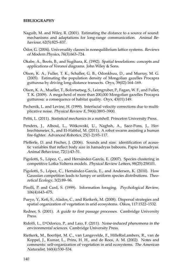
BIBLIOGRAPHY
Naguib, M. and Wiley, R. (2001). Estimating the distance to a source of sound:mechanisms and adaptations for long-range communication. Animal Be-haviour, 62(5):825–837.
Odor, G. (2004). Universality classes in nonequilibrium lattice systems. Reviewsof Modern Physics, 76(3):663–724.
Okabe, A., Boots, B., and Sugihara, K. (1992). Spatial tesselations: concepts andapplications of Voronoi diagrams. John Wiley & Sons.
Olson, K. A., Fuller, T. K., Schaller, G. B., Odonkhuu, D., and Murray, M. G.(2005). Estimating the population density of Mongolian gazelles Procapragutturosa by driving long-distance transects. Oryx, 39(02):164–169.
Olson, K. A., Mueller, T., Bolortsetseg, S., Leimgruber, P., Fagan, W. F., and Fuller,T. K. (2009). A mega-herd of more than 200,000 Mongolian gazelles Procapragutturosa: a consequence of habitat quality. Oryx, 43(01):149.
Pechenik, L. and Levine, H. (1999). Interfacial velocity corrections due to multi-plicative noise. Physical Review E, 59(4):3893–3900.
Peliti, L. (2011). Statistical mechanics in a nutshell. Princeton University Press.
Penders, J., Alboul, L., Witkowski, U., Naghsh, A., Saez-Pons, J., Her-brechtsmeier, S., and El-Habbal, M. (2011). A robot swarm assisting a humanfire-fighter. Advanced Robotics, 25(1-2):93–117.
Pfefferle, D. and Fischer, J. (2006). Sounds and size: identification of acous-tic variables that reflect body size in hamadryas baboons, Papio hamadryas.Animal Behaviour, 72(1):43–51.
Pigolotti, S., Lopez, C., and Hernandez-Garcıa, E. (2007). Species clustering incompetitive Lotka-Volterra models. Physical Review Letters, 98(25):258101.
Pigolotti, S., Lopez, C., Hernandez-Garcıa, E., and Andersen, K. (2010). HowGaussian competition leads to lumpy or uniform species distributions. Theo-retical Ecology, 3(2):89–96.
Pirolli, P. and Card, S. (1999). Information foraging. Psychological Review,106(4):643–675.
Pueyo, Y., Kefi, S., Alados, C., and Rietkerk, M. (2008). Dispersal strategies andspatial organization of vegetation in arid ecosystems. Oikos, 117:1522–1532.
Redner, S. (2001). A guide to first passage processes. Cambridge UniversityPress.
Ridolfi, L., D’Odorico, P., and Laio, F. (2011). Noise-induced phenomena in theenvironmental sciences. Cambridge University Press.
Rietkerk, M., Boerlijst, M. C., van Langevelde, F., HilleRisLambers, R., van deKoppel, J., Kumar, L., Prins, H. H., and de Roos, A. M. (2002). Notes andcomments: self-organization of vegetation in arid ecosystems. The AmericanNaturalist, 160(4):530–534.
140
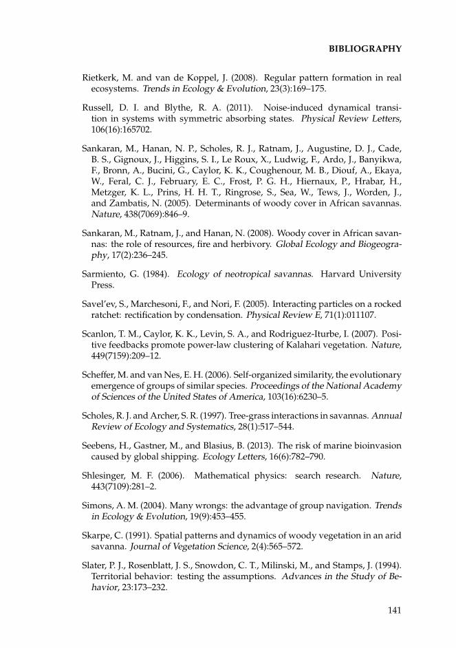
BIBLIOGRAPHY
Rietkerk, M. and van de Koppel, J. (2008). Regular pattern formation in realecosystems. Trends in Ecology & Evolution, 23(3):169–175.
Russell, D. I. and Blythe, R. A. (2011). Noise-induced dynamical transi-tion in systems with symmetric absorbing states. Physical Review Letters,106(16):165702.
Sankaran, M., Hanan, N. P., Scholes, R. J., Ratnam, J., Augustine, D. J., Cade,B. S., Gignoux, J., Higgins, S. I., Le Roux, X., Ludwig, F., Ardo, J., Banyikwa,F., Bronn, A., Bucini, G., Caylor, K. K., Coughenour, M. B., Diouf, A., Ekaya,W., Feral, C. J., February, E. C., Frost, P. G. H., Hiernaux, P., Hrabar, H.,Metzger, K. L., Prins, H. H. T., Ringrose, S., Sea, W., Tews, J., Worden, J.,and Zambatis, N. (2005). Determinants of woody cover in African savannas.Nature, 438(7069):846–9.
Sankaran, M., Ratnam, J., and Hanan, N. (2008). Woody cover in African savan-nas: the role of resources, fire and herbivory. Global Ecology and Biogeogra-phy, 17(2):236–245.
Sarmiento, G. (1984). Ecology of neotropical savannas. Harvard UniversityPress.
Savel’ev, S., Marchesoni, F., and Nori, F. (2005). Interacting particles on a rockedratchet: rectification by condensation. Physical Review E, 71(1):011107.
Scanlon, T. M., Caylor, K. K., Levin, S. A., and Rodriguez-Iturbe, I. (2007). Posi-tive feedbacks promote power-law clustering of Kalahari vegetation. Nature,449(7159):209–12.
Scheffer, M. and van Nes, E. H. (2006). Self-organized similarity, the evolutionaryemergence of groups of similar species. Proceedings of the National Academyof Sciences of the United States of America, 103(16):6230–5.
Scholes, R. J. and Archer, S. R. (1997). Tree-grass interactions in savannas. AnnualReview of Ecology and Systematics, 28(1):517–544.
Seebens, H., Gastner, M., and Blasius, B. (2013). The risk of marine bioinvasioncaused by global shipping. Ecology Letters, 16(6):782–790.
Shlesinger, M. F. (2006). Mathematical physics: search research. Nature,443(7109):281–2.
Simons, A. M. (2004). Many wrongs: the advantage of group navigation. Trendsin Ecology & Evolution, 19(9):453–455.
Skarpe, C. (1991). Spatial patterns and dynamics of woody vegetation in an aridsavanna. Journal of Vegetation Science, 2(4):565–572.
Slater, P. J., Rosenblatt, J. S., Snowdon, C. T., Milinski, M., and Stamps, J. (1994).Territorial behavior: testing the assumptions. Advances in the Study of Be-havior, 23:173–232.
141
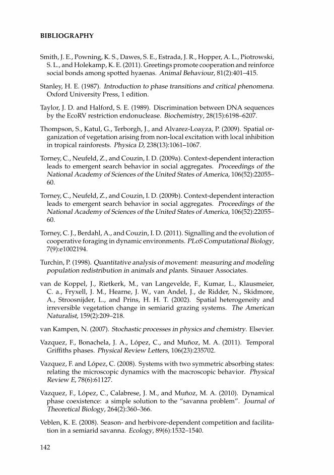
BIBLIOGRAPHY
Smith, J. E., Powning, K. S., Dawes, S. E., Estrada, J. R., Hopper, A. L., Piotrowski,S. L., and Holekamp, K. E. (2011). Greetings promote cooperation and reinforcesocial bonds among spotted hyaenas. Animal Behaviour, 81(2):401–415.
Stanley, H. E. (1987). Introduction to phase transitions and critical phenomena.Oxford University Press, 1 edition.
Taylor, J. D. and Halford, S. E. (1989). Discrimination between DNA sequencesby the EcoRV restriction endonuclease. Biochemistry, 28(15):6198–6207.
Thompson, S., Katul, G., Terborgh, J., and Alvarez-Loayza, P. (2009). Spatial or-ganization of vegetation arising from non-local excitation with local inhibitionin tropical rainforests. Physica D, 238(13):1061–1067.
Torney, C., Neufeld, Z., and Couzin, I. D. (2009a). Context-dependent interactionleads to emergent search behavior in social aggregates. Proceedings of theNational Academy of Sciences of the United States of America, 106(52):22055–60.
Torney, C., Neufeld, Z., and Couzin, I. D. (2009b). Context-dependent interactionleads to emergent search behavior in social aggregates. Proceedings of theNational Academy of Sciences of the United States of America, 106(52):22055–60.
Torney, C. J., Berdahl, A., and Couzin, I. D. (2011). Signalling and the evolution ofcooperative foraging in dynamic environments. PLoS Computational Biology,7(9):e1002194.
Turchin, P. (1998). Quantitative analysis of movement: measuring and modelingpopulation redistribution in animals and plants. Sinauer Associates.
van de Koppel, J., Rietkerk, M., van Langevelde, F., Kumar, L., Klausmeier,C. a., Fryxell, J. M., Hearne, J. W., van Andel, J., de Ridder, N., Skidmore,A., Stroosnijder, L., and Prins, H. H. T. (2002). Spatial heterogeneity andirreversible vegetation change in semiarid grazing systems. The AmericanNaturalist, 159(2):209–218.
van Kampen, N. (2007). Stochastic processes in physics and chemistry. Elsevier.
Vazquez, F., Bonachela, J. A., Lopez, C., and Munoz, M. A. (2011). TemporalGriffiths phases. Physical Review Letters, 106(23):235702.
Vazquez, F. and Lopez, C. (2008). Systems with two symmetric absorbing states:relating the microscopic dynamics with the macroscopic behavior. PhysicalReview E, 78(6):61127.
Vazquez, F., Lopez, C., Calabrese, J. M., and Munoz, M. A. (2010). Dynamicalphase coexistence: a simple solution to the “savanna problem”. Journal ofTheoretical Biology, 264(2):360–366.
Veblen, K. E. (2008). Season- and herbivore-dependent competition and facilita-tion in a semiarid savanna. Ecology, 89(6):1532–1540.
142
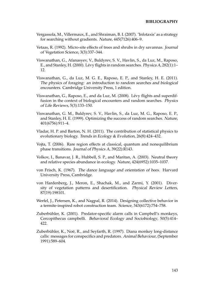
BIBLIOGRAPHY
Vergassola, M., Villermaux, E., and Shraiman, B. I. (2007). ’Infotaxis’ as a strategyfor searching without gradients. Nature, 445(7126):406–9.
Vetaas, R. (1992). Micro-site effects of trees and shrubs in dry savannas. Journalof Vegetation Science, 3(3):337–344.
Viswanathan, G., Afanasyev, V., Buldyrev, S. V., Havlin, S., da Luz, M., Raposo,E., and Stanley, H. (2000). Levy flights in random searches. Physica A, 282(1):1–12.
Viswanathan, G., da Luz, M. G. E., Raposo, E. P., and Stanley, H. E. (2011).The physics of foraging: an introduction to random searches and biologicalencounters. Cambridge University Press, 1 edition.
Viswanathan, G., Raposo, E., and da Luz, M. (2008). Levy flights and superdif-fusion in the context of biological encounters and random searches. Physicsof Life Reviews, 5(3):133–150.
Viswanathan, G. M., Buldyrev, S. V., Havlin, S., da Luz, M. G., Raposo, E. P.,and Stanley, H. E. (1999). Optimizing the success of random searches. Nature,401(6756):911–4.
Vladar, H. P. and Barton, N. H. (2011). The contribution of statistical physics toevolutionary biology. Trends in Ecology & Evolution, 26(8):424–432.
Vojta, T. (2006). Rare region effects at classical, quantum and nonequilibriumphase transitions. Journal of Physics A, 39(22):R143.
Volkov, I., Banavar, J. R., Hubbell, S. P., and Maritan, A. (2003). Neutral theoryand relative species abundance in ecology. Nature, 424(6952):1035–1037.
von Frisch, K. (1967). The dance language and orientation of bees. HarvardUniversity Press, Cambridge.
von Hardenberg, J., Meron, E., Shachak, M., and Zarmi, Y. (2001). Diver-sity of vegetation patterns and desertification. Physical Review Letters,87(19):198101.
Werfel, J., Petersen, K., and Nagpal, R. (2014). Designing collective behavior ina termite-inspired robot construction team. Science, 343(6172):754–758.
Zuberbuhler, K. (2001). Predator-specific alarm calls in Campbell’s monkeys,Cercopithecus campbelli. Behavioral Ecology and Sociobiology, 50(5):414–422.
Zuberbuhler, K., Noe, R., and Seyfarth, R. (1997). Diana monkey long-distancecalls: messages for conspecifics and predators. Animal Behaviour, (September1991):589–604.
143


Curriculum Vitae
Personal Details
Gender: Male.
Date of birth: 2nd February, 1988.
Place of birth: Pontevedra, Spain.
Mobile Phone: +34-626-880035
Citizenship: Spanish.
I.D Number: 78851298-F
e-mail: [email protected]
Webpage: http://ifisc.uib-csic.es/˜ricardo/
Research Interests
Statistical physics, complex systems, biological physics,spatial ecology, theoretical biology, stochastic processes, pattern formation, col-lective behavior of active matter and quantum theory.
Current Position
Ph.D. Student.Center: Spanish National Research Council (CSIC)-University of the BalearicIslands (UIB).Institute: IFISC, Institute for Cross Disciplinary Physics and Complex Systems.
Campus Universitat Illes Balears,E-07122 Palma de Mallorca, Spain.Phone:+34-971-259881
Occupational status: Predoctoral fellowship. Dedication: Full time.
145
Education
10/2006–06/2010 Licenciatura in Physics. Specialization in Fundamental Physics.University of La Laguna (Spain) (Spanish equivalent to Bach-elor degree).
10/2010–09/2011 Master in Physics. University of the Balearic Islands (Spain).
Since 10/2010 Ph.D. student at the Institute for Cross Disciplinary Physicsand Complex Systems (CSIC-UIB).
Supervisor: Dr. Cristobal Lopez.
Long Stays (more than 4 weeks):
03/2012–06/2012 Smithsonian Conservation Biology Institute. Front Royal VA,USA.
Ecology Center.
Supervisor: Dr. Justin Calabrese.
07/2011–08/2011 Max-Planck Institute for the Physics of Complex Systems.Dresden, Germany.
Biological Physics group.
Supervisor: Dr. Federico Vazquez.
Short Visits:
26–28/02/2014 Institute for Chemistry and Biology of the Marine Environ-ment. Carl von Ossietzky University. Oldenburg, Germany.
Invited by Prof. Bernd Blasius.
Previous Positions:
10/2009–06/2010 Undergraduate collaborator at Department for FundamentalPhysics II. University of La Laguna (Spain).
Supervisor: Dr. Santiago Brouard
07/2009–09/2009 Summer internship. Institute for Cross Disciplinary Physicsand Complex Systems, Palma (Spain).
Supervisor: Dr. Cristobal Lopez and Dr. Federico Vazquez.
146
01/2009–06/2009 Collaboration at the Faculty of Physics of the University ofLa Laguna (Spain).
Supervisor: Dr. Santiago Brouard
Publications in Peer-Reviewed Journals:
1. R. Martınez-Garcıa, J.M Calabrese, E. Hernandez-Garcıa, and C. Lopez.Minimal mechanisms for vegetation patterns in semiarid regions. Re-viewed and resubmitted to Philosophical Transactions of the Royal SocietyA. (arXiv:1402.1077), (2014).
2. R. Martınez-Garcıa, J.M Calabrese, and C. Lopez. Optimal search in inter-acting populations: Gaussian jumps versus Levy flights. Physical ReviewE, 89, 032718, (2014).
3. R. Martınez-Garcıa, J.M Calabrese, E. Hernandez-Garcıa, and C. Lopez.Vegetation pattern formation in semiarid systems without facilitative mech-anisms. Geophysical Research Letters,40, 6143–6147, (2013).
4. R. Martınez-Garcıa, J.M Calabrese and C. Lopez. Spatial patterns in mesicsavannas: the local facilitation limit and the role of demographic stochas-ticity. Journal of Theoretical Biology, 333, 156-165, (2013).
5. R. Martınez-Garcıa, J.M Calabrese, T. Mueller, K.A. Olson and C. Lopez.Optimizing the search for resources by sharing information: Mongoliangazelles as a case study. Physical Review Letters, 110, 248106, (2013).
• Highlighted as Physics Focus in the webpage of the American PhysicalSociety.
• Commented on Physics World (www.physicsworld.com).
• Commented on The Hindu (Indian general newspaper).
• Highlighted by the Spanish Royal Society of Physics in the section“Fısica al dıa” of its webpage.
• Commented on the local press, Diario de Mallorca.
6. R. Martınez-Garcıa, F. Vazquez, C. Lopez and M.A. Munoz. Temporaldisorder in up-down symmetric systems. Physical Review E, 85, 051125,(2012).
7. S. Brouard and R. Martınez. Cavity-mediated entanglement between dis-tant atoms: Effect of spatial dispersion. Physics Letters A. 375, 1640-1645,(2011).
147
Manuscripts in preparation
• C. Murgui, R. Martınez-Garcıa, C. Lopez, and E. Hernandez-Garcıa. Spatialaggregation in a population with two nonlocal interaction scales.
• R. Martınez-Garcıa, F. Vazquez and C. Lopez. Optimal search in an inter-acting population with informed and uninformed individuals.
Participation in Conferences and Seminars:
Oral presentation:
• III Conference of Physics Students. La Laguna, Spain. 18-19 March 2010.
Generating maximum entangled states between atoms.R. Martınez and S. Brouard.
• I Summer School on Statistical Physics of Complex and Small Systems.Palma, Spain. 12-23 September 2011.
Temporal Griffiths Phases.R. Martınez-Garcıa, F. Vazquez, J.A. Bonachela, C. Lopez and M.A. Munoz.
• Search and Stochastic Phenomena in Complex Physical and Biological Sys-tems. Palma, Spain. 28 May - 1 June 2012.
A nonlocal spatial model for savannas.R. Martınez-Garcıa and C. Lopez.
• Models in Population Dynamics and Ecology. Osnabruck, Germany. 26-29August 2013.
Optimizing the search for resources sharing information. The case of Mon-golian Gazelles.R. Martınez-Garcıa, J.M. Calabrese, T. Mueller, K.A. Olson and C. Lopez.
• III Summer School on Statistical Physics of Complex and Small Systems.Palma, Spain. 2-13, Sept. 2013.
Optimizing the search for resources sharing information. The case of Mon-golian Gazelles.R. Martınez-Garcıa, J.M. Calabrese, T. Mueller, K.A. Olson and C. Lopez.
Poster:
• XVII FisEs. Barcelona, Spain. 2-4 June 2011.
Temporal Griffiths Phases.R. Martınez-Garcıa, F. Vazquez, J.A. Bonachela, C. Lopez and M.A. Munoz.
148
• XVIII FisEs.. Palma, Spain. 18-20 October 2012.
A nonlocal spatial model for savannas.
R. Martınez-Garcıa, J.M. Calabrese and C. Lopez.
• XVIII FisEs.. Palma, Spain. 18-20 October 2012.
A long range interaction model for foragers.
R. Martınez-Garcıa, J.M. Calabrese, T. Mueller, K.A. Olson and C. Lopez.
• STATPHYS25. Seoul, Republic of Korea, 22-26 July 2013.
Optimizing the search for resources sharing information. The case of Mon-golian Gazelles.
R. Martınez-Garcıa, J.M. Calabrese, T. Mueller, K.A. Olson and C. Lopez.
• Models in Population Dynamics and Ecology. Osnabruck, Germany. 26-29August 2013.
Spatial patterns in mesic savannas: The local facilitation limit and the roleof demographic stochasticity.
R. Martınez-Garcıa, J.M. Calabrese and C. Lopez.
• III Summer School on Statistical Physics of Complex and Small Systems.Palma, Spain. 2-13, Sept. 2013.
Optimizing the search for resources sharing information. The case of Mon-golian Gazelles.
R. Martınez-Garcıa, J.M. Calabrese, T. Mueller, K.A. Olson and C. Lopez.
• XIX FisEs. Ourense, Spain. 2-4, April 2014.
Vegetation pattern formation in semiarid systems without facilitative mech-anisms.
R. Martınez-Garcıa, J.M. Calabrese, E. Hernandez-Garcıa and C. Lopez.
• EGU General Assembly. Vienna, Austria. 28 April-2 May 2014.
Vegetation pattern formation in semiarid systems induced by long-rangecompetition in the absence of facilitation mechanisms.
R. Martınez-Garcıa, J.M. Calabrese, E. Hernandez-Garcıa and C. Lopez.
Contributions presented by coauthors:
• XIX FisEs. Ourense, Spain. 2-4, April 2014. (Oral presentation: C. Lopez)
Optimizing the search for resources by sharing information: Mongoliangazelles as case study.
R. Martınez-Garcıa, J.M. Calabrese, T. Mueller, K.A. Olson and C. Lopez.
149
Given Seminars:
• Institute for Chemistry and Biology of the Marine Environment. Carl vonOssietzky University. Oldenburg, Germany. 27 February 2014.
Optimizing the search for resources sharing information: the Mongoliangazelle.R. Martınez-Garcıa, J.M. Calabrese, T. Mueller, K.A. Olson and C. Lopez.
• IFISC Seminar. Palma, Spain. 22 January 2014.
Vegetation patterns. The role of nonlocal interactions.
• IFISC Seminar. Palma, Spain. 12 February 2013.
Searching with communication: the case of the Mongolian gazelle.R. Martınez-Garcıa, J.M. Calabrese, T. Mueller, K.A. Olson and C. Lopez.
• Seminar of the Faculty of Physics of the University of La Laguna. 20December 2011.
The effect of temporal disorder in complex systems.R. Martınez-Garcıa, F. Vazquez and C. Lopez.
Seminars and Courses Attendance:
• III Summer School on Statistical Physics of Complex and Small Systems.Institute for Cross Disciplinary Physics and Complex Systems. Palma,Spain. 2-13, Sept. 2013.
• Massive Open Online Course Introduction to Complexity. Santa Fe Insti-tute, 2013.
• I Summer School on Statistical Physics of Complex and Small Systems.Institute for Cross Disciplinary Physics and Complex Systems. Palma,Spain. 12-23, Sept. 2011.
• 47th Winter School of Theoretical Physics. Simple Models for ComplexSystems. Institute for Theoretical Physics. Wroclaw, Poland. 7-11 Feb.2011.
• Utrecht Summer School, H2 Theoretical Physics. Institute for TheoreticalPhysics. Utrecht, the Netherlands. 16 – 27 Aug. 2010.
• Computational Methods on Astrophysics Calculus. IDL programming.University of La Laguna, Spain. Sept 2009 – Jan 2010. (60 hours)
• Modern Optics Days. Institute for Cross Disciplinary Physics and ComplexSystems. Palma, Spain. 6-10 July 2009
• I Conference of Physics Students. University of La Laguna. 3-4 April 2008
150

Fellowships and Academic Awards:
2014 Montserrat Casas award in the category of Sciences, Engi-neering and Architecture (4000e).
2013 Banco Santander-UIB award to the best PhD students of theUniversity of the Balearic Islands (1500e).
2010–2014 JAE-Predoc predoctoral fellowship. Spanish National Re-search Council (CSIC).
2010 III Conference of Physics Students. University of La Laguna.Best Oral presentation Award from Scientific Committee.
09/2009–06/2010 Collaboration Fellowship from the Spanish Ministery of Ed-ucation (3000e).
07/2009–08/2009 JAE-Intro fellowship. Spanish National Research Council.
2006 International Physics Olympiads. Bronze Medal on SpanishNational round.
2006 Graduated with honours on High School Education (Sci-ences).
Mentorship Experience:
07/2013–08/2013 Co-supervisor of an Intro-IFISC 2013 grant.
Ms. Clara Murgui.
Computer skills and competences:
• Programming Languages: Fortran, IDL, LATEX, Mathematica, Gnuplot,Bash, Grace.
• Operating systems: Windows, Linux.
• User of computer cluster and European Grid Infrastructure.
Participation in Research Projects:
Since 2013 Complex Systems Physics: Information, Technology, Societyand Ecology (INTENSE@COSYP). FIS2012-30634.
P.I: Prof. Maxi San Miguel
151
2010–2013 Fisica Interdisciplinar y de Sistemas Complejos. (FISICOS).FIS2007-60327.
P.I: Prof. Maxi San Miguel
Academic Referee:
Physical Review Letters, Ecological Modelling, Physical Review E.
Language Skills:
Spanish: Mother tongue.
Galician: Second mother tongue.
English: London Examinations. Level 5. Proficient Communication.
German: European A1.1 Level.
French: Elementary level.
Society Membership:
Since 2014 Society of Mathematical Biology.
Since 2014 European Society of Mathematical and Theoretical Biology.
Since 2012 Optical Society of America.
Palma de Mallorca, 2nd May 2014.
152