State space modelsOutline 1ARIMA models in state space form 2RegARMA models in state space form 3The...
72
Rob J Hyndman State space models 3: ARIMA and RegARMA models, and dlm
Transcript of State space modelsOutline 1ARIMA models in state space form 2RegARMA models in state space form 3The...
Rob J Hyndman
State space models
3: ARIMA and RegARMA models, and dlm
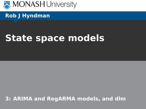
Outline
1 ARIMA models in state space form
2 RegARMA models in state space form
3 The dlm package for R
4 MLE using the dlm package
5 Filtering, smoothing and forecasting usingthe dlm package
6 Final remarks
State space models 3: ARIMA and RegARMA models, and dlm 2
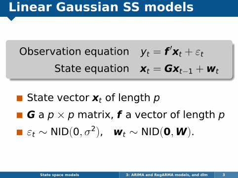
Linear Gaussian SS models
Observation equation yt = f ′xt + εt
State equation xt = Gxt−1 + wt
State vector xt of length p
G a p× p matrix, f a vector of length p
εt ∼ NID(0, σ2), wt ∼ NID(0,W).
State space models 3: ARIMA and RegARMA models, and dlm 3

Outline
1 ARIMA models in state space form
2 RegARMA models in state space form
3 The dlm package for R
4 MLE using the dlm package
5 Filtering, smoothing and forecasting usingthe dlm package
6 Final remarks
State space models 3: ARIMA and RegARMA models, and dlm 4
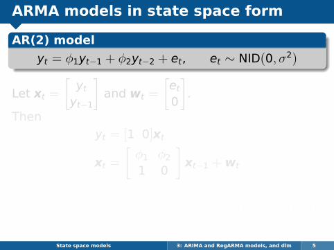
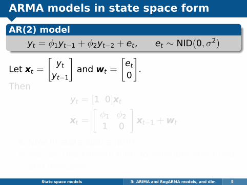
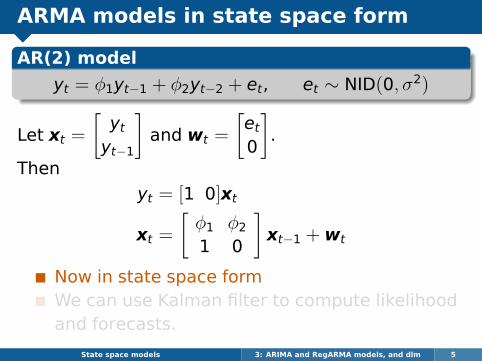
ARMA models in state space form
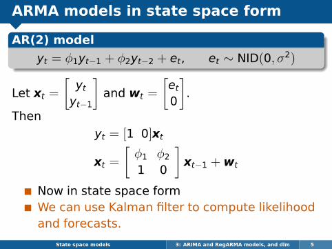
AR(2) model
yt = φ1yt−1 + φ2yt−2 + et, et ∼ NID(0, σ2)
Let xt =
[ytyt−1
]and wt =
[et0
].
Then
yt = [1 0]xt
xt =
[φ1 φ2
1 0
]xt−1 + wt
Now in state space formWe can use Kalman filter to compute likelihoodand forecasts.
State space models 3: ARIMA and RegARMA models, and dlm 5
ARMA models in state space form
AR(2) model
yt = φ1yt−1 + φ2yt−2 + et, et ∼ NID(0, σ2)
Let xt =
[ytyt−1
]and wt =
[et0
].
Then
yt = [1 0]xt
xt =
[φ1 φ2
1 0
]xt−1 + wt
Now in state space formWe can use Kalman filter to compute likelihoodand forecasts.
State space models 3: ARIMA and RegARMA models, and dlm 5

ARMA models in state space form
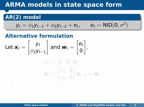
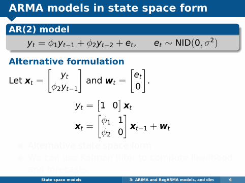
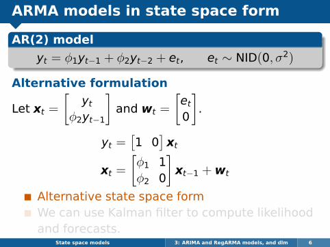
AR(2) model
yt = φ1yt−1 + φ2yt−2 + et, et ∼ NID(0, σ2)
Alternative formulation
Let xt =
[yt
φ2yt−1
]and wt =
[et0
].
yt =[1 0
]xt
xt =
[φ1 1φ2 0
]xt−1 + wt
Alternative state space formWe can use Kalman filter to compute likelihoodand forecasts.
State space models 3: ARIMA and RegARMA models, and dlm 6
ARMA models in state space form
AR(2) model
yt = φ1yt−1 + φ2yt−2 + et, et ∼ NID(0, σ2)
Alternative formulation
Let xt =
[yt
φ2yt−1
]and wt =
[et0
].
yt =[1 0
]xt
xt =
[φ1 1φ2 0
]xt−1 + wt
Alternative state space formWe can use Kalman filter to compute likelihoodand forecasts.
State space models 3: ARIMA and RegARMA models, and dlm 6

ARMA models in state space form
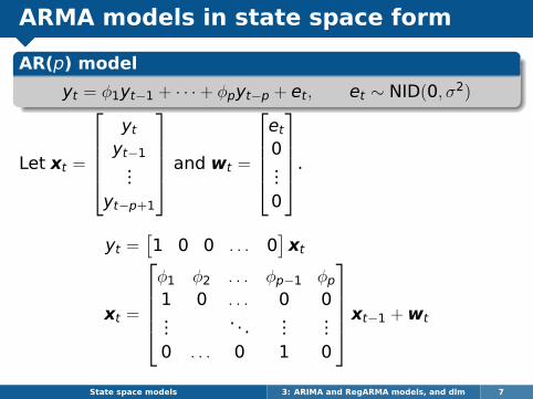
AR(p) model
yt = φ1yt−1 + · · ·+ φpyt−p + et, et ∼ NID(0, σ2)
Let xt =
ytyt−1
...yt−p+1
and wt =
et0...0
.
yt =[1 0 0 . . . 0
]xt
xt =
φ1 φ2 . . . φp−1 φp1 0 . . . 0 0...
. . ....
...0 . . . 0 1 0
xt−1 + wt
State space models 3: ARIMA and RegARMA models, and dlm 7
ARMA models in state space form
AR(p) model
yt = φ1yt−1 + · · ·+ φpyt−p + et, et ∼ NID(0, σ2)
Let xt =
ytyt−1
...yt−p+1
and wt =
et0...0
.
yt =[1 0 0 . . . 0
]xt
xt =
φ1 φ2 . . . φp−1 φp1 0 . . . 0 0...
. . ....
...0 . . . 0 1 0
xt−1 + wt
State space models 3: ARIMA and RegARMA models, and dlm 7
ARMA models in state space form
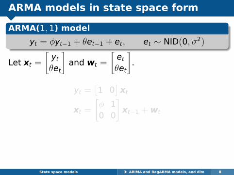
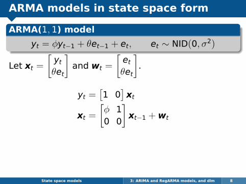
ARMA(1,1) model
yt = φyt−1 + θet−1 + et, et ∼ NID(0, σ2)
Let xt =
[ytθet
]and wt =
[etθet
].
yt =[1 0
]xt
xt =
[φ 10 0
]xt−1 + wt
State space models 3: ARIMA and RegARMA models, and dlm 8
ARMA models in state space form
ARMA(1,1) model
yt = φyt−1 + θet−1 + et, et ∼ NID(0, σ2)
Let xt =
[ytθet
]and wt =
[etθet
].
yt =[1 0
]xt
xt =
[φ 10 0
]xt−1 + wt
State space models 3: ARIMA and RegARMA models, and dlm 8
ARMA models in state space form
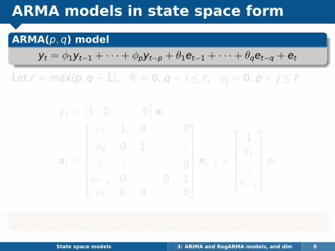
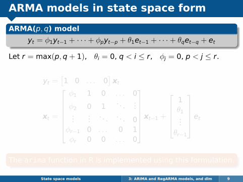
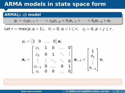
ARMA(p,q) model
yt = φ1yt−1 + · · ·+ φpyt−p + θ1et−1 + · · ·+ θqet−q + et
Let r = max(p,q+ 1), θi = 0, q < i ≤ r, φj = 0, p < j ≤ r.
yt =[1 0 . . . 0
]xt
xt =
φ1 1 0 . . . 0
φ2 0 1. . .
......
.... . . . . . 0
φr−1 0 . . . 0 1φr 0 0 . . . 0
xt−1 +
1θ1...
θr−1
et
The arima function in R is implemented using this formulation.
State space models 3: ARIMA and RegARMA models, and dlm 9
ARMA models in state space form
ARMA(p,q) model
yt = φ1yt−1 + · · ·+ φpyt−p + θ1et−1 + · · ·+ θqet−q + et
Let r = max(p,q+ 1), θi = 0, q < i ≤ r, φj = 0, p < j ≤ r.
yt =[1 0 . . . 0
]xt
xt =
φ1 1 0 . . . 0
φ2 0 1. . .
......
.... . . . . . 0
φr−1 0 . . . 0 1φr 0 0 . . . 0
xt−1 +
1θ1...
θr−1
et
The arima function in R is implemented using this formulation.
State space models 3: ARIMA and RegARMA models, and dlm 9
Outline
1 ARIMA models in state space form
2 RegARMA models in state space form
3 The dlm package for R
4 MLE using the dlm package
5 Filtering, smoothing and forecasting usingthe dlm package
6 Final remarks
State space models 3: ARIMA and RegARMA models, and dlm 10
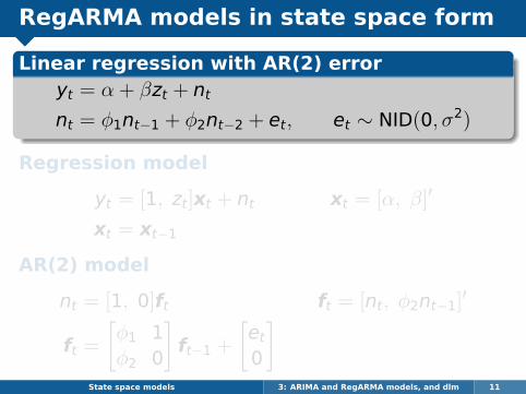
RegARMA models in state space form
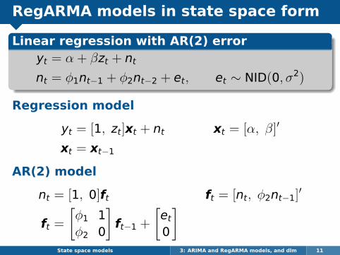
Linear regression with AR(2) erroryt = α + βzt + ntnt = φ1nt−1 + φ2nt−2 + et, et ∼ NID(0, σ2)
Regression model
yt = [1, zt]xt + nt xt = [α, β]′
xt = xt−1
AR(2) model
nt = [1, 0]ft ft = [nt, φ2nt−1]′
ft =
[φ1 1φ2 0
]ft−1 +
[et0
]State space models 3: ARIMA and RegARMA models, and dlm 11
RegARMA models in state space form
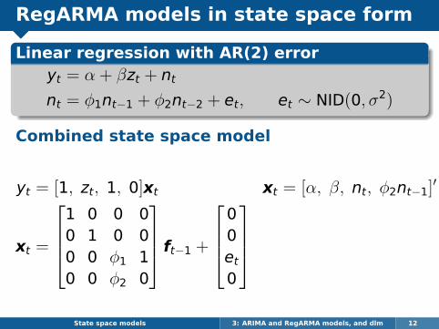
Linear regression with AR(2) erroryt = α + βzt + ntnt = φ1nt−1 + φ2nt−2 + et, et ∼ NID(0, σ2)
Regression model
yt = [1, zt]xt + nt xt = [α, β]′
xt = xt−1
AR(2) model
nt = [1, 0]ft ft = [nt, φ2nt−1]′
ft =
[φ1 1φ2 0
]ft−1 +
[et0
]State space models 3: ARIMA and RegARMA models, and dlm 11
RegARMA models in state space form
Linear regression with AR(2) erroryt = α + βzt + ntnt = φ1nt−1 + φ2nt−2 + et, et ∼ NID(0, σ2)
Combined state space model
yt = [1, zt, 1, 0]xt xt = [α, β, nt, φ2nt−1]′
xt =
1 0 0 00 1 0 00 0 φ1 10 0 φ2 0
ft−1 +
00et0
State space models 3: ARIMA and RegARMA models, and dlm 12
RegARMA models in state space form
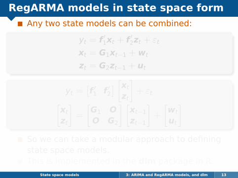
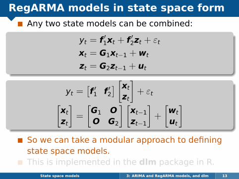
Any two state models can be combined:
yt = f ′1xt + f ′2zt + εtxt = G1xt−1 + wt
zt = G2zt−1 + ut
yt =[f ′1 f ′2
] [xt
zt
]+ εt[
xt
zt
]=
[G1 OO G2
] [xt−1
zt−1
]+
[wt
ut
]So we can take a modular approach to definingstate space models.This is implemented in the dlm package in R.
State space models 3: ARIMA and RegARMA models, and dlm 13
RegARMA models in state space form
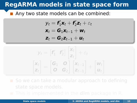
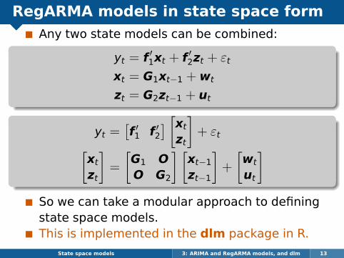
Any two state models can be combined:
yt = f ′1xt + f ′2zt + εtxt = G1xt−1 + wt
zt = G2zt−1 + ut
yt =[f ′1 f ′2
] [xt
zt
]+ εt[
xt
zt
]=
[G1 OO G2
] [xt−1
zt−1
]+
[wt
ut
]So we can take a modular approach to definingstate space models.This is implemented in the dlm package in R.
State space models 3: ARIMA and RegARMA models, and dlm 13

RegARMA models in state space form
Any two state models can be combined:
yt = f ′1xt + f ′2zt + εtxt = G1xt−1 + wt
zt = G2zt−1 + ut
yt =[f ′1 f ′2
] [xt
zt
]+ εt[
xt
zt
]=
[G1 OO G2
] [xt−1
zt−1
]+
[wt
ut
]So we can take a modular approach to definingstate space models.This is implemented in the dlm package in R.
State space models 3: ARIMA and RegARMA models, and dlm 13

Outline
1 ARIMA models in state space form
2 RegARMA models in state space form
3 The dlm package for R
4 MLE using the dlm package
5 Filtering, smoothing and forecasting usingthe dlm package
6 Final remarks
State space models 3: ARIMA and RegARMA models, and dlm 14
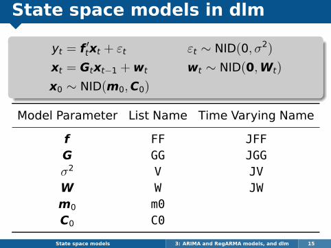
State space models in dlm
yt = f ′txt + εt εt ∼ NID(0, σ2)
xt = Gtxt−1 + wt wt ∼ NID(0,Wt)
x0 ∼ NID(m0,C0)
Model Parameter List Name Time Varying Name
f FF JFFG GG JGGσ2 V JVW W JWm0 m0C0 C0
State space models 3: ARIMA and RegARMA models, and dlm 15
State space models in dlm
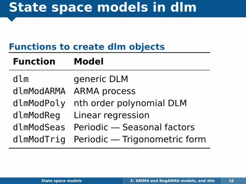
Functions to create dlm objects
Function Model
dlm generic DLMdlmModARMA ARMA processdlmModPoly nth order polynomial DLMdlmModReg Linear regressiondlmModSeas Periodic — Seasonal factorsdlmModTrig Periodic — Trigonometric form
State space models 3: ARIMA and RegARMA models, and dlm 16
Local level model
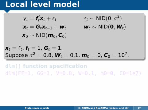
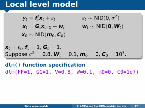
yt = f ′txt + εt εt ∼ NID(0, σ2)
xt = Gtxt−1 + wt wt ∼ NID(0,Wt)
x0 ∼ NID(m0,C0)
xt = `t, ft = 1, Gt = 1.Suppose σ2 = 0.8, Wt = 0.1, m0 = 0, C0 = 107.
dlm() function specificationdlm(FF=1, GG=1, V=0.8, W=0.1, m0=0, C0=1e7)
State space models 3: ARIMA and RegARMA models, and dlm 17
Local level model
yt = f ′txt + εt εt ∼ NID(0, σ2)
xt = Gtxt−1 + wt wt ∼ NID(0,Wt)
x0 ∼ NID(m0,C0)
xt = `t, ft = 1, Gt = 1.Suppose σ2 = 0.8, Wt = 0.1, m0 = 0, C0 = 107.
dlm() function specificationdlm(FF=1, GG=1, V=0.8, W=0.1, m0=0, C0=1e7)
State space models 3: ARIMA and RegARMA models, and dlm 17

Local level model
yt = f ′txt + εt εt ∼ NID(0, σ2)
xt = Gtxt−1 + wt wt ∼ NID(0,Wt)
x0 ∼ NID(m0,C0)
xt = `t, ft = 1, Gt = 1.Suppose σ2 = 0.8, Wt = 0.1, m0 = 0, C0 = 107.
dlm() function specificationdlm(FF=1, GG=1, V=0.8, W=0.1, m0=0, C0=1e7)
dlmModPoly() function specification
dlmModPoly(order=1, dV=0.8, dW=0.1)
State space models 3: ARIMA and RegARMA models, and dlm 18

Local level model
> mod <- dlmModPoly(order=1, dV=.8, dW=.1)
> names(mod)
[1] "m0" "C0" "FF" "V" "GG" "W" "JFF" "JV" "JGG" "JW"
> FF(mod)
[,1]
[1,] 1
> GG(mod)
[,1]
[1,] 1
> class(mod)
[1] "dlm"
State space models 3: ARIMA and RegARMA models, and dlm 19
Local trend model
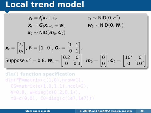
yt = f ′txt + εt εt ∼ NID(0, σ2)
xt = Gtxt−1 + wt wt ∼ NID(0,Wt)
x0 ∼ NID(m0,C0)
xt =
[`tbt
], ft =
[1 0
], Gt =
[1 10 1
].
Suppose σ2 = 0.8, Wt =
[0.2 00 0.1
], m0 =
[00
], C0 =
[107 00 107
]dlm() function specificationdlm(FF=matrix(c(1,0),nrow=1),GG=matrix(c(1,0,1,1),ncol=2),V=0.8, W=diag(c(0.2,0.1)),m0=c(0,0), C0=diag(c(1e7,1e7)))
State space models 3: ARIMA and RegARMA models, and dlm 20

Local trend model
yt = f ′txt + εt εt ∼ NID(0, σ2)
xt = Gtxt−1 + wt wt ∼ NID(0,Wt)
x0 ∼ NID(m0,C0)
xt =
[`tbt
], ft =
[1 0
], Gt =
[1 10 1
].
Suppose σ2 = 0.8, Wt =
[0.2 00 0.1
], m0 =
[00
], C0 =
[107 00 107
]dlm() function specificationdlm(FF=matrix(c(1,0),nrow=1),GG=matrix(c(1,0,1,1),ncol=2),V=0.8, W=diag(c(0.2,0.1)),m0=c(0,0), C0=diag(c(1e7,1e7)))
State space models 3: ARIMA and RegARMA models, and dlm 20
Local trend model
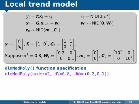
yt = f ′txt + εt εt ∼ NID(0, σ2)
xt = Gtxt−1 + wt wt ∼ NID(0,Wt)
x0 ∼ NID(m0,C0)
xt =
[`tbt
], ft =
[1 0
], Gt =
[1 10 1
].
Suppose σ2 = 0.8, Wt =
[0.2 00 0.1
], m0 =
[00
], C0 =
[107 00 107
]dlmModPoly() function specificationdlmModPoly(order=2, dV=0.8, dW=c(0.2,0.1))
State space models 3: ARIMA and RegARMA models, and dlm 21
Time varying regression model
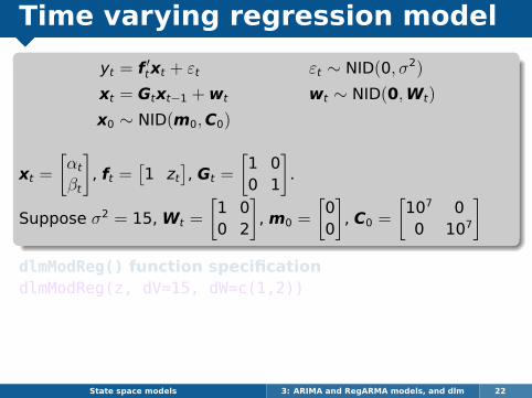
yt = f ′txt + εt εt ∼ NID(0, σ2)
xt = Gtxt−1 + wt wt ∼ NID(0,Wt)
x0 ∼ NID(m0,C0)
xt =
[αt
βt
], ft =
[1 zt
], Gt =
[1 00 1
].
Suppose σ2 = 15, Wt =
[1 00 2
], m0 =
[00
], C0 =
[107 00 107
]dlmModReg() function specificationdlmModReg(z, dV=15, dW=c(1,2))
State space models 3: ARIMA and RegARMA models, and dlm 22

Time varying regression model
yt = f ′txt + εt εt ∼ NID(0, σ2)
xt = Gtxt−1 + wt wt ∼ NID(0,Wt)
x0 ∼ NID(m0,C0)
xt =
[αt
βt
], ft =
[1 zt
], Gt =
[1 00 1
].
Suppose σ2 = 15, Wt =
[1 00 2
], m0 =
[00
], C0 =
[107 00 107
]dlmModReg() function specificationdlmModReg(z, dV=15, dW=c(1,2))
State space models 3: ARIMA and RegARMA models, and dlm 22

Linear regression with AR(2) errors
yt = α + βzt + ntnt = φ1nt−1 + φ2nt−2 + et, et ∼ NID(0,u)
State space models 3: ARIMA and RegARMA models, and dlm 23
Linear regression with AR(2) errors
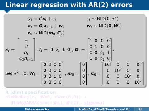
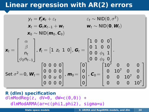
yt = f ′txt + εt εt ∼ NID(0, σ2)
xt = Gtxt−1 + wt wt ∼ NID(0,Wt)
x0 ∼ NID(m0,C0)
xt =
αβnt
φ2nt−1
, ft =[1 zt 1 0
], Gt =
1 0 0 00 1 0 00 0 φ1 10 0 φ2 0
.
Set σ2=0, Wt=
0 0 0 00 0 0 00 0 u 00 0 0 0
, m0=
0000
, C0=
107 0 0 00 107 0 00 0 107 00 0 0 107
R (dlm) specificationdlmModReg(z, dV=0, dW=c(0,0)) +
dlmModARMA(ar=c(phi1,phi2), sigma=u)State space models 3: ARIMA and RegARMA models, and dlm 24
Linear regression with AR(2) errors
yt = f ′txt + εt εt ∼ NID(0, σ2)
xt = Gtxt−1 + wt wt ∼ NID(0,Wt)
x0 ∼ NID(m0,C0)
xt =
αβnt
φ2nt−1
, ft =[1 zt 1 0
], Gt =
1 0 0 00 1 0 00 0 φ1 10 0 φ2 0
.
Set σ2=0, Wt=
0 0 0 00 0 0 00 0 u 00 0 0 0
, m0=
0000
, C0=
107 0 0 00 107 0 00 0 107 00 0 0 107
R (dlm) specificationdlmModReg(z, dV=0, dW=c(0,0)) +
dlmModARMA(ar=c(phi1,phi2), sigma=u)State space models 3: ARIMA and RegARMA models, and dlm 24
Outline
1 ARIMA models in state space form
2 RegARMA models in state space form
3 The dlm package for R
4 MLE using the dlm package
5 Filtering, smoothing and forecasting usingthe dlm package
6 Final remarks
State space models 3: ARIMA and RegARMA models, and dlm 25

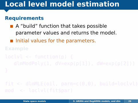
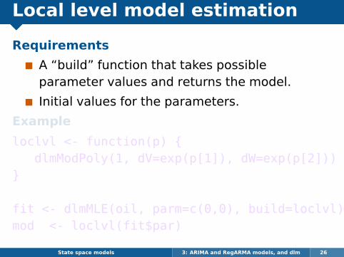
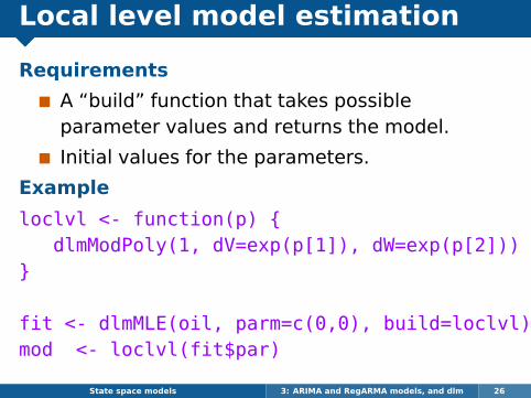
Local level model estimation
Requirements
A “build” function that takes possibleparameter values and returns the model.
Initial values for the parameters.
Example
loclvl <- function(p) {dlmModPoly(1, dV=exp(p[1]), dW=exp(p[2]))
}
fit <- dlmMLE(oil, parm=c(0,0), build=loclvl)mod <- loclvl(fit$par)
State space models 3: ARIMA and RegARMA models, and dlm 26
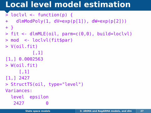
Local level model estimation> loclvl <- function(p) {+ dlmModPoly(1, dV=exp(p[1]), dW=exp(p[2]))+ }> fit <- dlmMLE(oil, parm=c(0,0), build=loclvl)> mod <- loclvl(fit$par)> V(oil.fit)
[,1][1,] 0.0002563> W(oil.fit)
[,1][1,] 2427> StructTS(oil, type="level")Variances:level epsilon2427 0
State space models 3: ARIMA and RegARMA models, and dlm 27
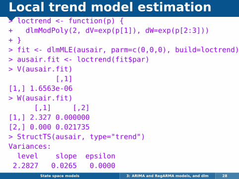
Local trend model estimation> loctrend <- function(p) {+ dlmModPoly(2, dV=exp(p[1]), dW=exp(p[2:3]))+ }> fit <- dlmMLE(ausair, parm=c(0,0,0), build=loctrend)> ausair.fit <- loctrend(fit$par)> V(ausair.fit)
[,1][1,] 1.6563e-06> W(ausair.fit)
[,1] [,2][1,] 2.327 0.000000[2,] 0.000 0.021735> StructTS(ausair, type="trend")Variances:level slope epsilon2.2827 0.0265 0.0000
State space models 3: ARIMA and RegARMA models, and dlm 28
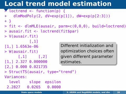
Local trend model estimation> loctrend <- function(p) {+ dlmModPoly(2, dV=exp(p[1]), dW=exp(p[2:3]))+ }> fit <- dlmMLE(ausair, parm=c(0,0,0), build=loctrend)> ausair.fit <- loctrend(fit$par)> V(ausair.fit)
[,1][1,] 1.6563e-06> W(ausair.fit)
[,1] [,2][1,] 2.327 0.000000[2,] 0.000 0.021735> StructTS(ausair, type="trend")Variances:level slope epsilon2.2827 0.0265 0.0000
Different initialization andoptimization choices oftengiven different parameterestimates.
State space models 3: ARIMA and RegARMA models, and dlm 28
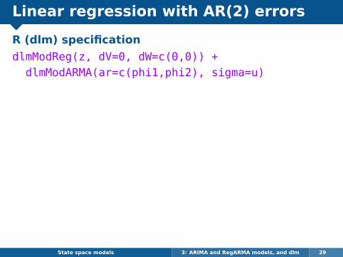
Linear regression with AR(2) errors
R (dlm) specification
dlmModReg(z, dV=0, dW=c(0,0)) +dlmModARMA(ar=c(phi1,phi2), sigma=u)
State space models 3: ARIMA and RegARMA models, and dlm 29

Linear regression with AR(2) errors
R (dlm) specification
dlmModReg(z, dV=0, dW=c(0,0)) +dlmModARMA(ar=c(phi1,phi2), sigma=u)
MLEregar2 <- function(p) {
dlmModReg(z, dV=.0001, dW=c(0,0)) +dlmModARMA(ar=c(p[1],p[2]), sigma=exp(p[3]))
}z <- usconsumption[,1]fit <- dlmMLE(usconsumption[,2], parm=c(0,0,0),
build=regar2)mod <- regar2(fit$par)
State space models 3: ARIMA and RegARMA models, and dlm 30
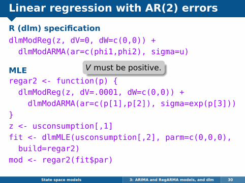
Linear regression with AR(2) errors
R (dlm) specification
dlmModReg(z, dV=0, dW=c(0,0)) +dlmModARMA(ar=c(phi1,phi2), sigma=u)
MLEregar2 <- function(p) {
dlmModReg(z, dV=.0001, dW=c(0,0)) +dlmModARMA(ar=c(p[1],p[2]), sigma=exp(p[3]))
}z <- usconsumption[,1]fit <- dlmMLE(usconsumption[,2], parm=c(0,0,0),
build=regar2)mod <- regar2(fit$par)
V must be positive.
State space models 3: ARIMA and RegARMA models, and dlm 30
BSM model
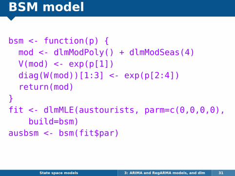
bsm <- function(p) {mod <- dlmModPoly() + dlmModSeas(4)V(mod) <- exp(p[1])diag(W(mod))[1:3] <- exp(p[2:4])return(mod)
}fit <- dlmMLE(austourists, parm=c(0,0,0,0),
build=bsm)ausbsm <- bsm(fit$par)
State space models 3: ARIMA and RegARMA models, and dlm 31
Outline
1 ARIMA models in state space form
2 RegARMA models in state space form
3 The dlm package for R
4 MLE using the dlm package
5 Filtering, smoothing and forecasting usingthe dlm package
6 Final remarks
State space models 3: ARIMA and RegARMA models, and dlm 32
More dlm functions
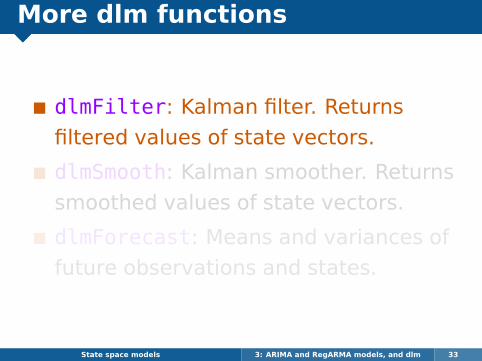
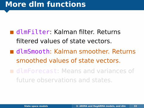
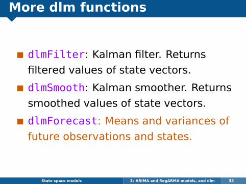
dlmFilter: Kalman filter. Returns
filtered values of state vectors.
dlmSmooth: Kalman smoother. Returns
smoothed values of state vectors.
dlmForecast: Means and variances of
future observations and states.
State space models 3: ARIMA and RegARMA models, and dlm 33
More dlm functions
dlmFilter: Kalman filter. Returns
filtered values of state vectors.
dlmSmooth: Kalman smoother. Returns
smoothed values of state vectors.
dlmForecast: Means and variances of
future observations and states.
State space models 3: ARIMA and RegARMA models, and dlm 33
More dlm functions
dlmFilter: Kalman filter. Returns
filtered values of state vectors.
dlmSmooth: Kalman smoother. Returns
smoothed values of state vectors.
dlmForecast: Means and variances of
future observations and states.
State space models 3: ARIMA and RegARMA models, and dlm 33
BSM model
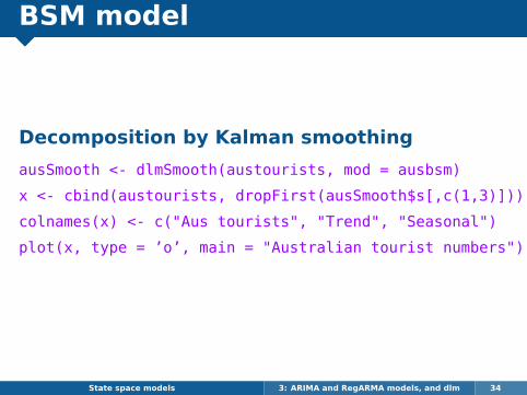
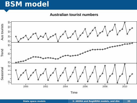
Decomposition by Kalman smoothing
ausSmooth <- dlmSmooth(austourists, mod = ausbsm)
x <- cbind(austourists, dropFirst(ausSmooth$s[,c(1,3)]))
colnames(x) <- c("Aus tourists", "Trend", "Seasonal")
plot(x, type = ’o’, main = "Australian tourist numbers")
State space models 3: ARIMA and RegARMA models, and dlm 34
BSM model
●
●
●●
●
●
●
●●
●
●●
●
●
●●
●
●
●
●
●
●●
●
●
●
●
●
●
●
●
●
●
●
●●
●
●
●●
●
●
●
●
●
●
●
●
2030
4050
60
Aus
tour
ists
● ● ● ●●
●●
● ● ● ●● ● ● ● ● ● ●
●●
● ●● ● ● ●
●●
●●
●● ● ● ● ● ●
●● ● ● ● ●
●● ● ● ●
2535
45
Tren
d
●
●
●
●
●
●
●
●
●
●
●●
●
●
●
●
●
●
●
●
●
●
●
●
●
●
●
●
●
●
●
●
●
●
●
●
●
●
●
●
●
●
●
●
●
●
●
●
−10
05
10
2000 2002 2004 2006 2008 2010
Sea
sona
l
Time
Australian tourist numbers
State space models 3: ARIMA and RegARMA models, and dlm 35
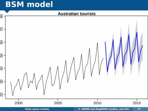
BSM model
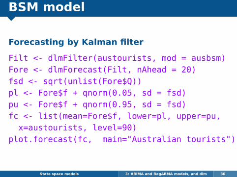
Forecasting by Kalman filter
Filt <- dlmFilter(austourists, mod = ausbsm)Fore <- dlmForecast(Filt, nAhead = 20)fsd <- sqrt(unlist(Fore$Q))pl <- Fore$f + qnorm(0.05, sd = fsd)pu <- Fore$f + qnorm(0.95, sd = fsd)fc <- list(mean=Fore$f, lower=pl, upper=pu,
x=austourists, level=90)plot.forecast(fc, main="Australian tourists")
State space models 3: ARIMA and RegARMA models, and dlm 36
BSM modelAustralian tourists
2000 2005 2010 2015
2030
4050
6070
80
State space models 3: ARIMA and RegARMA models, and dlm 37
Outline
1 ARIMA models in state space form
2 RegARMA models in state space form
3 The dlm package for R
4 MLE using the dlm package
5 Filtering, smoothing and forecasting usingthe dlm package
6 Final remarks
State space models 3: ARIMA and RegARMA models, and dlm 38
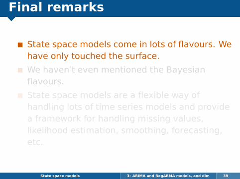
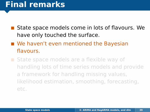
Final remarks
State space models come in lots of flavours. Wehave only touched the surface.
We haven’t even mentioned the Bayesianflavours.
State space models are a flexible way ofhandling lots of time series models and providea framework for handling missing values,likelihood estimation, smoothing, forecasting,etc.
State space models 3: ARIMA and RegARMA models, and dlm 39
Recommended References
1 RJ Hyndman, AB Koehler, J Keith Ord, andRD Snyder (2008). Forecasting withexponential smoothing: the state spaceapproach. Springer
2 AC Harvey (1989). Forecasting, structuraltime series models and the Kalman filter.Cambridge University Press
3 J Durbin and SJ Koopman (2001). Time seriesanalysis by state space methods. OxfordUniversity Press
4 G Petris, S Petrone, and P Campagnoli (2009).Dynamic Linear Models with R. Springer
State space models 3: ARIMA and RegARMA models, and dlm 40
Contact details
www.robjhyndman.com
State space models 3: ARIMA and RegARMA models, and dlm 41