Starfish - Particle In Cell · 2018-05-28 · Particle In Cell Consulting LLC Starfish User’s...
42
User’s Guide Starfish 2D Plasma / Gas Simulation Program Version 0.18 January 28 th , 2018 Particle In Cell Consulting LLC particleincell.com [email protected]
Transcript of Starfish - Particle In Cell · 2018-05-28 · Particle In Cell Consulting LLC Starfish User’s...

User’s Guide
Starfish
2D Plasma / Gas Simulation Program
Version 0.18
January 28th, 2018
Particle In Cell Consulting LLC
particleincell.com [email protected]

Particle In Cell Consulting LLC Starfish User’s Guide
2
Contents I. Introduction .................................................................................................................................................................... 4
I.a) License ..................................................................................................................................................................... 4
I.b) Getting Started ........................................................................................................................................................ 4
I.c) Input File Structure ................................................................................................................................................. 5
II. Numerical Model ............................................................................................................................................................ 5
III. Examples ..................................................................................................................................................................... 6
III.a) Flow of plasma past a charged cylinder .................................................................................................................. 6
III.b) Supersonic expansion of atmospheric gas to vacuum .......................................................................................... 19
IV. Extending Starfish-LE ................................................................................................................................................ 23
V. Bugs and Future Work .................................................................................................................................................. 24
VI. Command Reference ................................................................................................................................................ 25
VI.a) General .................................................................................................................................................................. 25
VI.a.1) NOTE ............................................................................................................................................................. 25
VI.a.2) LOG ................................................................................................................................................................ 25
VI.a.3) RESTART ........................................................................................................................................................ 26
VI.a.4) STARFISH ....................................................................................................................................................... 26
VI.a.5) STOP .............................................................................................................................................................. 26
VI.a.6) TIME .............................................................................................................................................................. 26
VI.b) Input / Output ....................................................................................................................................................... 27
VI.b.1) ANIMATION ................................................................................................................................................... 27
VI.b.2) AVERAGING ................................................................................................................................................... 27
VI.b.3) LOAD_FIELD ................................................................................................................................................... 27
VI.b.4) OUTPUT ......................................................................................................................................................... 28
VI.b.5) PARTICLE_TRACE ........................................................................................................................................... 29
VI.b.6) STATS ............................................................................................................................................................. 29
VI.c) Materials ............................................................................................................................................................... 30
VI.c.1) MATERIALS .................................................................................................................................................... 30
VI.c.2) MATERIAL ...................................................................................................................................................... 30
VI.d) Material Interactions ............................................................................................................................................ 32
VI.d.1) MATERIAL_INTERACTIONS ............................................................................................................................ 32
VI.d.2) SURFACE_HIT ................................................................................................................................................ 32
VI.d.3) DSMC ............................................................................................................................................................. 32
VI.d.4) MCC ............................................................................................................................................................... 33
VI.d.5) CHEMISTRY .................................................................................................................................................... 33
Particle In Cell Consulting LLC Starfish User’s Guide
3
VI.e) Boundaries ............................................................................................................................................................ 34
VI.e.1) BOUNDARIES ................................................................................................................................................. 34
VI.e.2) BOUNDARY .................................................................................................................................................... 35
VI.f) Domain .................................................................................................................................................................. 36
VI.f.1) DOMAIN ........................................................................................................................................................ 36
VI.f.2) MESH ............................................................................................................................................................. 36
VI.g) Sources .................................................................................................................................................................. 37
VI.g.1) SOURCES ....................................................................................................................................................... 37
VI.g.2) BOUNDARY_SOURCE..................................................................................................................................... 37
VI.h) Solver..................................................................................................................................................................... 39
VI.h.1) SOLVER .......................................................................................................................................................... 39
VII. Data Fields ................................................................................................................................................................. 40
VII.a) Mesh Data ......................................................................................................................................................... 40
VII.a.1) General .......................................................................................................................................................... 40
VII.a.2) Material-Specific (base.mat) ......................................................................................................................... 40
VII.a.3) MCC ............................................................................................................................................................... 41
VII.a.4) DSMC ............................................................................................................................................................. 41
VII.b) Boundary Data .................................................................................................................................................. 41
VII.b.1) Material-Specific ........................................................................................................................................... 41
VIII. References ................................................................................................................................................................ 42

Particle In Cell Consulting LLC Starfish User’s Guide
4
I. Introduction
Starfish is a two-dimensional XY/RZ plasma and gas simulation code written in Java [1]. The code was developed with generality in mind, allowing it to consider a wide range of gas dynamics problems. The current version mainly implements functionality needed for simulations of low-density plasmas using the Particle In Cell Method (PIC) with MCC/DSMC collisions. Rudimentary support for fluid modeling is also implemented and we are working on extending this functionality as soon as possible. Starfish operates on structured 2D Cartesian or body fitted stretched meshes. Surface geometry is included via linear or cubic splines. The code is easily extensible using plugins, as described later in this document. Starfish consists of two version. The Light Edition (Starfish-LE) is the main code described in this document. It implements numerical models needed to perform simple gas kinetics simulations. The binary and source code for this version can be downloaded by visiting https://www.particleincell.com/starfish. The full version (Starfish-Full) implements various proprietary models mainly for modeling ion sources and surface interactions. The full version is not publicly available.
I.a) License Please review LICENSE included with the code. Your use of the code implies consent to the license agreement. In general, you are allowed to use the code for any non-commercial purpose assuming the original copyright notice is preserved.
I.b) Getting Started Although we started working on the GUI, a working version of GUI is not yet available. For now, Starfish is run from the command line. You need to have a Java Run Time1 environment installed on your system. To use the code, navigate to the directory containing the simulation input files. To run the code, type java -jre <path_to_starfish-LE.jar> For instance, if your starfish-LE.jar file is located in a folder “codes/starfish-LE” in your home directory, and if the case you wanted to run was located in a subfolder “dat/tutorial/step1”, you would do the following: > cd starfish-LE > cd dat/tutorial/step1 > java -jar ../../../starfish-LE.jar
Figure 1. Starfish running on Microsoft Windows in Windows PowerShell (left) and Cygwin (right)
1 Java JRE can be downloaded from https://java.com/en/download/
Particle In Cell Consulting LLC Starfish User’s Guide
5
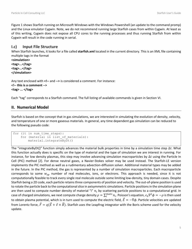
Figure 1 shows Starfish running on Microsoft Windows with the Windows Powershell (an update to the command promp) and the Linux emulator Cygwin. Note, we do not recommend running large Starfish cases from within Cygwin. At least as of this writing, Cygwin does not expose all CPU cores to the running processes and thus running Starfish from within Cygwin will result in the code running in serial.
I.c) Input File Structure When Starfish launches, it looks for a file called starfish.xml located in the current directory. This is an XML file containing multiple tags in the format <simulation> <tag>...</tag> <tag>...</tag> </simulation> Any text enclosed with <!-- and --> is considered a comment. For instance: <!-- this is a comment --> <tag> ... </tag> Each “tag” corresponds to a Starfish command. The full listing of available commands is given in Section VI.
II. Numerical Model
Starfish is based on the concept that in gas simulations, we are interested in simulating the evolution of density, velocity, and temperature of one or more gaseous materials. In general, any time dependent gas simulation can be reduced to the following pseudo code: for (it in num_time_steps):
for (material in list_of_materials):
material.integrateByDt()
The “integrateByDt()” function simply advances the material bulk properties in time by a simulation time step Δ𝑡. What this function actually does is specific on the type of material and the type of simulation we are interest in running. For instance, for low density plasmas, this step may involve advancing simulation macroparticles by Δ𝑡 using the Particle In Cell (PIC) method [2]. For dense neutral gases, a Navier-Stokes solver may be used instead. The Starfish-LE version implements the PIC method as well as a rudimentary advection-diffusion solver. Additional material types may be added in the future. In the PIC method, the gas is represented by a number of simulation macroparticles. Each macroparticle corresponds to some 𝑤𝑠𝑝 number of real molecules, ions, or electrons. This approach is needed, since it is not
computationally feasible to track every single real molecule outside some limiting low-density, tiny domain cases. Despite Starfish being a 2D code, each particle retains three components of position and velocity. The out-of-plane position is used to rotate the particle back to the computational slice in axisymmetric simulations. Particle positions in the simulation plane are then used to compute number density of material “i” 𝑛𝑖 by scattering particle positions to a computational grid. In
case of charged simulations, we next compute charge density 𝜌 = ∑ 𝑛𝑖𝑚𝑎𝑡𝑠𝑖 . Poisson’s equation, 𝜖0∇
2𝜙 = −𝜌 is then used
to obtain plasma potential, which is in turn used to compute the electric field, �⃗� = −∇𝜙. Particle velocities are updated
from Lorentz force, 𝐹 = 𝑞(�⃗� + 𝑣 × �⃗� ). Starfish uses the Leapfrog integrator with the Boris scheme used for the velocity update.

Particle In Cell Consulting LLC Starfish User’s Guide
6
III. Examples
III.a) Flow of plasma past a charged cylinder We demonstrate the use of Starfish by summarizing a tutorial that was previously posted to the PIC-C blog2. In this simulation we will investigate the flow of plasma over an infinitely long charged cylinder.
Step 1: Computational Domain and Initial Field
We start the tutorial by specifying the computational domain, loading the problem geometry, solving plasma potential, and outputting results. No particles are introduced yet. The output that we will generate is shown in Figure 2.
Figure 2. The initial plasma potential on a 2D mesh and as a slice along Y=0.
As noted earlier, Starfish looks for a file named starfish.xml located in the current directory. This file contains all the commands that drive the simulation. The file used to produce the above output is shown below: <simulation>
<note>Starfish Tutorial: Part 1</note>
<!-- load input files -->
<load>domain.xml</load>
<load>materials.xml</load>
<load>boundaries.xml</load>
<!-- set potential solver -->
<solver type="poisson">
<n0>1e12</n0>
<Te0>1.5</Te0>
<phi0>0</phi0>
<max_it>1e4</max_it>
</solver>
<!-- set time parameters -->
<time>
<num_it>1</num_it>
<dt>1e-6</dt>
2 https://www.particleincell.com/2012/starfish-tutorial-part1/

Particle In Cell Consulting LLC Starfish User’s Guide
7
</time>
<!-- run simulation -->
<starfish />
<!-- save results -->
<output type="2D" file_name="field.dat" format="tecplot">
<scalars>phi, efi, efj, rho, nd.O+</scalars>
</output>
<output type="1D" file_name="profile.dat" format="tecplot">
<mesh>mesh1</mesh>
<index>J=0</index>
<scalars>phi, efi, efj, rho, nd.o+</scalars>
</output>
<output type="boundaries" file_name="boundaries.dat" format="tecplot" />
</simulation>
As you can see, this file is an XML document and it contains a number of elements nested within the parent <simulation> element. We will now review these commands in detail Line 2: <note> The input file starts with the note command, which simply outputs the specified message to the screen and the log file. This is a convenient way to remind you what simulation case the code is running. Lines 5-7: <load> The file next contains three load commands. These commands load the specified file and place it into the XML tree at the current position. They are used to split a single input file into more manageable smaller chunks. This command is particularly handy for data reuse, for instance, to reuse commonly used material definitions and material interaction tables. We will go through the content of these in more detail below. Lines 10-15: <solver> Lines 10 through 15 contain the solver command. This command is used to specify the details of the solver that will be used in the simulation. Here we use the non-linear Poisson solver. The parameters specify the reference values for the Boltzmann electron model, as well as the maximum number of iterations for the linear solver. Other parameters can also be set, such as the tolerance, and the settings for the non-linear NR solver, but here we just use the defaults. You can see the value of these by looking in the log file. Lines 18-21: <time> We next set time control parameters. We tell the code to run for a total of zero iterations. We also specify the time step size, which in this case is ignored. Running for zero iterations instructs the code to solve the initial field, but it will not attempt to inject particles (assuming sources were defined).

Particle In Cell Consulting LLC Starfish User’s Guide
8
Line 24: <starfish> On line 24 we finally start the simulation with the starfish command. All commands before this one were simply specifying the inputs, now these are used to compute the solution. The input file parser will wait for the solver to finish before moving to the next command. Lines 27-37: <output> By itself, the starfish command does not produce any useful output. The computed results are stored internally in memory and must be saved to the output file for post-processing. This is done with the output command. Three types of output are supported: 2D, 1D, and Boundaries. The first saves data on the 2D computational mesh. The 1D type is similar but it saves only a subset of the mesh, one with a fixed I or J coordinate. The Boundaries output saves data along the simulation geometry. This plot is useful for outputting surface-type parameters such as erosion rate or surface flux. Here we use it to simply save the loaded object geometry. Domain File (domain.xml) We now return to line 5, and consider the domain specification. The domain file, domain.xml, contains the following: <domain type="xy">
<mesh type="uniform" name="mesh1">
<origin>-0.15,0</origin>
<spacing>5e-3, 5e-3</spacing>
<nodes>70, 40</nodes>
<mesh-bc wall="left" type="dirichlet" value="0" />
<mesh-bc wall="bottom" type="symmetry"/>
</mesh>
</domain>
One of the unique features of Starfish is its ability to load an arbitrary number of computational meshes (note this functionality is broken in 0.18 but is being worked on). These meshes can be either rectilinear or body fitted elliptic meshes. In this example, we specify just a single rectilinear mesh. We first tell the code that our geometry is in the Cartesian (XY) coordinate system. Starfish also supports axisymmetric (RZ) domains. The uniform Cartesian mesh is specified by providing the location of the origin, node spacing, and the number of nodes in the two coordinate directions. We also apply a mesh boundary condition by setting the left wall to a fixed 0V potential. This is needed in order to create a potential gradient between the ambient free space and the sphere. We also let the bottom face be symmetric since we are simulating only one half of the computational domain. Materials definition (materials.xml) Starfish does not contain any build database of materials or material interactions. This information must be provided by the user. Since we don’t have any particles in this first step, we don’t yet concern ourselves with the interactions, however, we need to define the materials that will be present in the simulation. The materials file contains the following: <!-- materials file -->
<materials>
<material name="O+" type="kinetic">
<molwt>16</molwt>
<charge>1</charge>
<spwt>5e9</spwt>
<init>nd_back=1e4</init>
</material>
Particle In Cell Consulting LLC Starfish User’s Guide
9
<material name="SS" type="solid">
<molwt>52.3</molwt>
</material>
</materials>
As you can see, we defined two materials: atomic oxygen ions and stainless steel. The atomic oxygen ions are kinetic. This material will be modeled with simulation particles within the particle in cell method. Starfish also supports fluid materials, which use Navier Stokes or MHD equations to propagate densities, as well as solid materials, which don’t change throughout the simulation. The parameters needed to specify a material will depend greatly on its type. For the kinetic oxygen ions, we specify the particle specific weight, the number of real particles each simulation macroparticle represents. This number will influence the number of simulation particles in the simulation. We also specify the background density. A non-zero background density is required whenever the Boltzmann electron model is used due to the presence of the logarithmic term. Geometry file (boundaries.xml) The final piece is the geometry file boundaries.xml, which is listed below: <boundaries>
<boundary name="cylinder" type="solid" value="-100" reverse="false">
<material>SS</material>
<path>M 0.05, 0 L 0.0475528, -0.0154508 0.0404508, -0.0293893 0.0293893, -0.0404508
0.0154508, -0.0475528 -9.18E-18, -0.05 -0.0154508, -0.0475528 -0.0293893, -0.0404508 -
0.0404508, -0.0293893 -0.0475528, -0.0154508 -0.05, 6.12E-18 -0.0475528, 0.0154508 -
0.0404508, 0.0293893 -0.0293893, 0.0404508 -0.0154508, 0.0475528 3.06E-18, 0.05
0.0154508, 0.0475528 0.0293893, 0.0404508 0.0404508, 0.0293893 0.0475528, 0.0154508
0.05, 0</path>
</boundary>
</boundaries>
Currently, simulation objects are specified via linear or cubic Bezier splines. It is possible that a future version of the code will include elementary building-block shapes and support for other file formats. The boundary contains a child field called path which provides the geometrical information about the spline. The syntax is similar to the SVG format, with the exception that cubic splines are specified by simply listing the points through which the spline will pass and the control knot points are omitted. Here we use linear components (L) to trace a circle. The ordering of the nodes matters, since the code will use the ordering to figure out which side of the segment is “internal” to the object. The internal side is assumed to lie on the “left”, hence the circle segments move counter-clockwise. This path was created with the included MakeCircle.java program. Mesh Generation Finally, a quick note about mesh generation. Right now, Starfish supports just the “staircase” or “sugarcube” method. The code simply uses the provided surface boundary to figure out which mesh nodes are internal, and these nodes are given the boundary condition of the surface spline. A more detailed method of using cut cells is still in development. You can see in Figure 3 below the staircasing effect. This plot is generated by visualizing the “type” data field. The nodes in red as flagged as internal and the ones in blue comprise the gas domain. It is important to check that node location was set correctly before launching the simulation.

Particle In Cell Consulting LLC Starfish User’s Guide
10
Figure 3. Internal nodes (in red) set with the sugarcubing algorithm
Step 2: Particles and Animation
We now add particles to our simulation. In order to add particles, we need to specify sources. Starfish supports two types of sources: volume and surface. Here we will use the latter. Surface sources create particles along geometry (boundary) splines according to a prescribed velocity distribution function (VDF) and the surface normal vector. In this example, we want the entire left domain boundary to act as a source injecting particles with uniform velocity. This setup then approximates the movement of the cylinder through undisturbed plasma, with the frame of reference moving with the cylinder. First, we need to add a new boundary to the boundaries.xml file: <boundaries>
<boundary name="cylinder" type="solid" value="-1" reverse="false">
<material>SS</material>
<path>...</path>
</path>
</boundary>
<boundary name="inlet" type="virtual" >
<path>M -0.15,0.2 L -0.15, 0</path>
</boundary>
</boundaries>
We named this spline “inlet” and it was given a type of virtual. This classification means that the boundary will not be used in generating the mesh intersections nor will it be seen by the particles. It is available for use by sources and also by probes (but more about probes later). This spline is simply a linear segment from the bottom left to the top left corner of the computation mesh. As you can see, it is 0.2m long. To add the source, we add the following command to starfish.xml (this command could also be placed in an external file and loaded with the <load> command): <!-- set sources -->
<sources>
<boundary_source name="space">
<type>uniform</type>
<material>O+</material>
<boundary>inlet</boundary>
<mdot>5.313e-11</mdot>

Particle In Cell Consulting LLC Starfish User’s Guide
11
<v_drift>10000</v_drift>
</boundary_source>
</sources>
Here you can see how the boundary comes into play. The source is given type uniform, which means that it produces particles with velocity equal to v_drift. The particles will be moving in the direction of the surface normal of the associated boundary, the inlet. If the boundary consisted of a number of individual splines, the particles would be moving according to the local normal. This source will generate O+ particles at mass flow rate of 5.313e-11 kg/s. You may be wondering how this number was determined. We want our plasma density in the free space to be 1012 m-3 to correspond with the potential solver electron model settings. The mass flow rate is given by the following expression:
�̇� = 𝑚𝑛𝑢𝐴 where the terms on the RHS correspond to the atomic mass (16 amu, per materials.xml file), number density (1e12 m-3), velocity (10,000 m/s), and source area (0.2 m2). In the Cartesian (XY) mode, the area is equal to the spline length, since unit depth is assumed. This expression gives us the value that is used in the simulation. Also, since we now have particles, we need to run for enough time steps to reach the steady state. In this case, 400 time steps will do the trick. We modify the time command as follows: <!-- set time parameters -->
<time>
<num_it>400</num_it>
<dt>2e-7</dt>
</time>
After you run the simulation, we obtain results like those visualized in Figure 4 and Figure 5 . We can see that a wake forms behind the cylinder. We can also clearly see the “reflection” of ions at the centerline, the line of symmetry. In reality, this reflection corresponds to the influx of particles from the opposite half of the simulation. This is best seen in the plot of the vertical velocity.
Figure 4. Ion density and ion vertical velocity

Particle In Cell Consulting LLC Starfish User’s Guide
12
Figure 5. Plasma potential for flow over a cylinder
These results show the final solution at the end of the simulation. These results correspond to the instantaneous steady state results. But what if we wanted to learn more about how the solution progressed? Or what if we had a time-dependent injection source? This is where animations come in. Animations direct the simulation to save results at a prescribed frequency during the course of the computation. Animations are specified by wrapping the standard output command in an animation command. See the website for a visualization of this data. <!-- save animation -->
<animation start_it="1" frequency="20">
<output type="2D" file_name="field_ani.dat" format="tecplot">
<scalars>phi,rho, nd.O+,u.O+,v.O+</scalars>
</output>
</animation>
Step 3: Surface Interactions
In the previous step, ions that collided with the cylinder were simply removed from the simulation. This is the default surface interaction that occurs if no other model is defined. It is only partially realistic. In reality, when low energy ions collide with a surface, they tend to pick up an electron from the surface and recombine into a neutral. In many plasma processes, surface recombination is the dominant plasma loss mechanism. Recombination in the gas itself is a three body process that is negligible at densities below 1e19 m-3. Although significantly lower than atmospheric pressure, this density is still several orders of magnitude higher than densities present in common space plasma applications. For instance, the ambient plasma density at the Low Earth Orbit is around 1e12 m-3. So while it is true that an ion “disappears” from the simulation on surface impact, the prior simulation does not conserve mass since the reflected neutral is not added. We now add surface recombination to our model. This is done via Starfish’s interactions module. This module handles interactions between all materials, either kinetic (handled by the PIC method), fluid (handled by the CFD/MHD solvers), or solid (making up the surfaces). We first create a new text file in the simulation directory called interactions.xml. The content of this file is <!-- material interactions file -->
<material_interactions>
<surface_hit source="O+" target="SS">
<product>O</product>
<model>cosine</model>
<c_accom>0.5</c_accom>
<c_rest>0.9</c_rest>
</surface_hit>
</material_interactions>

Particle In Cell Consulting LLC Starfish User’s Guide
13
and we load this file by adding <load>interactions.xml</load>
to starfish.xml. We also need to add a new material to the database – remember, Starfish does not contain any built-in materials. We add the following to materials.xml: <material name="O" type="kinetic">
<molwt>16</molwt>
<charge>0</charge>
<spwt>2e5</spwt>
</material>
Each material interaction involves at least three participants: source, target, and product. The distinction between sources and products becomes blurry when dealing with collisions. However, they are clearly distinct when dealing with surface interactions. In this case, the source is the “flying” component. The target is the material that the source hits – the material from which the surface is made of. The product is the material the source turns into after undergoing the impact. In this case, we have told the code to turn O+ ions into O atoms after colliding with Stainless Steel surfaces. When you look in the materials file, you will see that the specific weight of the oxygen atoms (O), 2e5, differs from the specific weight of the oxygen ions (O+), 5e5. The code takes this into account, and creates, on average, 2.5 atom particles per each impacting ion. You can test this out yourself by changing the value and seeing the number of particles change. The actual density of oxygen atoms will however stay the same, but the data will become noisier as the number of particles is reduced. This can be seen below in Figure 1.
Figure 6. Density of neutrals from surface recombination of impacting ions. Images compare the effect of specific weight on results: 2e5 (left), and 2e7 (right). Instantaneous results.
Material Interaction Model So far we have only told the code to turn O+ into O. However, we have yet to specify how the new particles will leave the surface. This is done via the model field. Even relatively smooth surface will contain irregularities on the atomic scale. Furthermore, in many cases, incoming molecules do not bounce off the surface like a tennis ball. Instead, they momentarily settle on the surface and then they are re-emitted in a direction that tends to follow Lambert’s cosine law. The cosine model models this behavior. The angle of the emitted particle will scale proportionally to the cosine of angle between the velocity vector and the surface normal. Some additional models that are available include specular and diffuse (random) reflection. The 𝑐𝑟𝑒𝑠𝑡 and 𝑐𝑎𝑐𝑐𝑜𝑚 fields control the post impact velocity. The coefficient of restitution, 𝑐𝑟𝑒𝑠𝑡 = 𝑣2/𝑣1 is primarily applicable to finite-sized dust particles and for molecular simulations we will usually keep it at 1. The coefficient of thermal accommodation specifies the fraction of incoming particles that will completely forget their
Particle In Cell Consulting LLC Starfish User’s Guide
14
incoming velocity and will instead come off with a velocity corresponding to the thermal velocity of the surface. The overall algorithm is as follows: v2 = v1*c_rest /*post impact velocity*/
R = random(); /*pick a random number in [0,1)*/
if (R<c_accom)
v2 = v_th*sampleMaxwellian();
/*create particle with velocity magnitude v2*/
Complex Interaction Types In the above example, all incoming ions turned into neutrals and were re-emitted. However, what if we wanted to model a situation where a fraction of particles stick to the surface, another fraction is reflected specularly, and only the final fraction is emitted according to the cosine law? This is quite easy in Starfish. Starfish allows you to define multiple interaction types with a prescribed probability of occurrence. As an example, let’s consider a more complex interactions file: <!-- material interactions file -->
<material_interactions>
<surface_hit source="O+" target="SS">
<product>O</product>
<model>cosine</model>
<prob>0.4</prob>
<c_accom>0.5</c_accom>
<c_rest>0.9</c_rest>
</surface_hit>
<surface_hit source="O+" target="SS">
<product>O</product>
<model>specular</model>
<prob>0.2</prob>
<c_accom>0</c_accom>
<c_rest>1.0</c_rest>
</surface_hit>
</material_interactions>
We have now specified two surface_hit fields. In addition, we added a new field called prob. This field gives the probability for each model. As you can see, these two probabilities add up to a value less than 1.0. This is OK, the remaining particles will be handled by default handler, one that absorbs incoming particles.
Step 4: Steady State, Surface Flux, and Data Averaging
We next learn how to export surface properties, such as surface flux and deposition rate. We will also set up averaging to obtain averaged field properties. In the previous step, we added surface recombination of ions into neutrals. The more complex surface model had a fraction of ions stick to the cylinder. Now let’s assume that we want to determine the rate with which ions are arriving at the object, and also how much stuff is sticking to it. These are just two examples of surface (boundary) properties that can be exported from the simulation.

Particle In Cell Consulting LLC Starfish User’s Guide
15
But before we start discussing surface flux, we need to introduce the concept of steady state. Many computer simulation methods, especially ones based on kinetic approaches, such as PIC and DSMC, work by integrating simulation particles forward in time from some known initial state. The simulation will initially pass through a transient state in which the results are constantly changing and are not indicative of the final steady solution. As such, we need to wait until steady state to start collection cumulative data. Starfish automatically waits until steady state before starting to collect properties such as surface flux. This is an important point to note if you want to export cumulative data. By default, the steady state is determined automatically. But you can also override it. As an example, here is a time command which instructs the code to assume that steady state is reached at time step 100. <time>
<num_it>500</num_it>
<dt>5e-7</dt>
<steady_state>100</steady_state>
</time>
One thing that occurs once steady state is reached is that the code will start collecting information about particles hitting surfaces. This includes properties such as flux of individual materials, as well as the mass deposition rate, corresponding to the particles that stick (are absorbed) to the surface. We can output these properties by adding list of variables to the output statement. The result is shown in Figure 7. <output type="boundaries" file_name="boundaries.dat" format="tecplot">
<scalars>flux.o+, flux-normal.o+, depflux.o+, flux, deprate, depflux</scalars>
</output>
Figure 7. Surface flux saved as surface (boundary) data.
Data Averaging Since results from kinetic codes are quite noisy, it is a good practice to average results over several time steps to get both smoother plots, and to eliminate outlier data arising from statistical noise. This is done in Starfish with the averaging command. The syntax is <!-- setup averaging -->
<averaging frequency="2">
<variables>phi, nd.o+, nd.o</variables>
Particle In Cell Consulting LLC Starfish User’s Guide
16
</averaging>
The averaging starts automatically at steady state, and new data will be added every 2 time steps. The variables lines lists the variables to be averaged. Since averaging data adds a computational overhead, the code averages just the variables that are specified here. These averaged values are then exported using the standard output command, with the caveat that the averaged versions will have the base ending in “-ave”. For instance, <!-- save results -->
<output type="2D" file_name="field.dat" format="tecplot">
<scalars>phi, phi-ave, rho, nd.o+, nd-ave.o+, u.o+, v.o+, nd.o, nd-ave.o, u.o,
v.o</scalars>
</output>
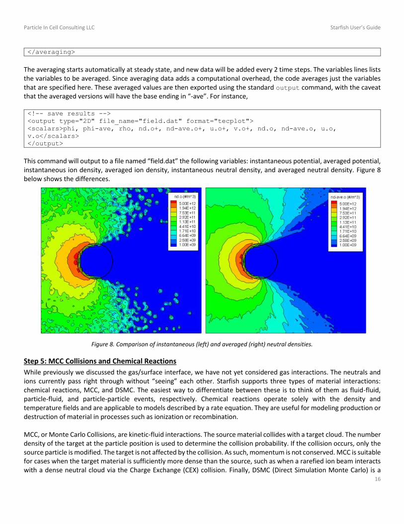
This command will output to a file named “field.dat” the following variables: instantaneous potential, averaged potential, instantaneous ion density, averaged ion density, instantaneous neutral density, and averaged neutral density. Figure 8 below shows the differences.
Figure 8. Comparison of instantaneous (left) and averaged (right) neutral densities.
Step 5: MCC Collisions and Chemical Reactions
While previously we discussed the gas/surface interface, we have not yet considered gas interactions. The neutrals and ions currently pass right through without “seeing” each other. Starfish supports three types of material interactions: chemical reactions, MCC, and DSMC. The easiest way to differentiate between these is to think of them as fluid-fluid, particle-fluid, and particle-particle events, respectively. Chemical reactions operate solely with the density and temperature fields and are applicable to models described by a rate equation. They are useful for modeling production or destruction of material in processes such as ionization or recombination. MCC, or Monte Carlo Collisions, are kinetic-fluid interactions. The source material collides with a target cloud. The number density of the target at the particle position is used to determine the collision probability. If the collision occurs, only the source particle is modified. The target is not affected by the collision. As such, momentum is not conserved. MCC is suitable for cases when the target material is sufficiently more dense than the source, such as when a rarefied ion beam interacts with a dense neutral cloud via the Charge Exchange (CEX) collision. Finally, DSMC (Direct Simulation Monte Carlo) is a

Particle In Cell Consulting LLC Starfish User’s Guide
17
kinetic-kinetic collision process. This method collides particles with other particles in the simulation cell. Both energy and momentum are conserved. This method is suitable for modeling collisions in like gases, such as to model momentum exchange (MEX) collisions in the ion gas. Starfish implements the No Time Counter (NTC) method of Bird [3]. DSMC is the most computationally demanding of these three methods. Material interactions are specified in the interactions file which you have already seen before. We used this file previously to add surface recombination. We modify the interactions file as follows: <material_interactions>
...
<!--
<chemistry model="ionization">
<sources>O,e-</sources>
<products>iO+,2*e-</products>
</chemistry> -->
<mcc model="cex">
<source>O+</source>
<target>O</target>
<sigma>inv</sigma>
<sigma_coeffs>1e-16</sigma_coeffs>
</mcc>
</material_interactions>
The chemistry interaction listed here within a comment illustrates how we go about modeling the ionization reaction
𝑂 + 𝑒− → 𝑂+ + 2𝑒− We can write this process as follows:
𝑑𝑛𝑂+ = +𝑘𝑛𝑂𝑛𝑒−𝑑𝑡 𝑑𝑛𝑂 = −𝑘𝑛𝑂+𝑛𝑒−𝑑𝑡
ignoring electron density change. Here “k” is the ionization rate (which is typically function of the electron temperature) and the two “n” correspond to the densities of the atoms and electrons. An example of this interaction is shown in Figure 9. We see that ions are created only in the region containing a neutral population. Additional details about the chemistry model are available online3.
Figure 9. Ions created by the ionization chemistry interaction
3 https://www.particleincell.com/2012/starfish-tutorial-part5/
Particle In Cell Consulting LLC Starfish User’s Guide
18
MCC Let’s now move onto MCC. Just as in the case of the chemical reaction, we specify the source and target, as well as the collision model. In this case, we’ll be using the CEX handler. This handler models the electron exchange between a fast ion and a slow neutral resulting in a fast neutral and a slow ion,
𝑂𝑓𝑎𝑠𝑡+ + 𝑂𝑠𝑙𝑜𝑤 → 𝑂𝑓𝑎𝑠𝑡 + 𝑂𝑠𝑙𝑜𝑤
+
But since this is MCC, we don’t actually modify the neutrals. Instead, the neutrals are used to compute the collision probability following 𝑃 = 1 − exp(−𝑛𝑛𝑔𝜎𝛥𝑡), where 𝑛𝑛 is the neutral density, 𝑔 is the relative velocity between the ion and the neutral (with the neutral assumed to be stationary), and 𝜎 is the collision cross-section. The sigma model is typically a function of relative velocity, with a number of models existing to describe different collision events. A classic model for modeling CEX is the model of Rapp and Francis. However here, for simplicity, we use a constant cross-section. But even with this relatively large value, collisions are still going to be a very rare event due to the low gas densities. So just to demonstrate this effect, let’s go ahead and specify a dense background neutral environment. In the materials file, let’s modify the oxygen atom by adding an init tag, <material name="O" type="kinetic">
<molwt>16</molwt>
<charge>0</charge>
<spwt>2e5</spwt>
<init>nd_back=2e18</init>
</material>
This background density will be added to any density from the actual kinetic particles. We can also turn off the potential solver. One way is to replace the Poisson solver with a constant electric field model with zero components, <!-- set zero electric field -->
<solver type="constant-ef">
<comps>0,0</comps>
</solver>
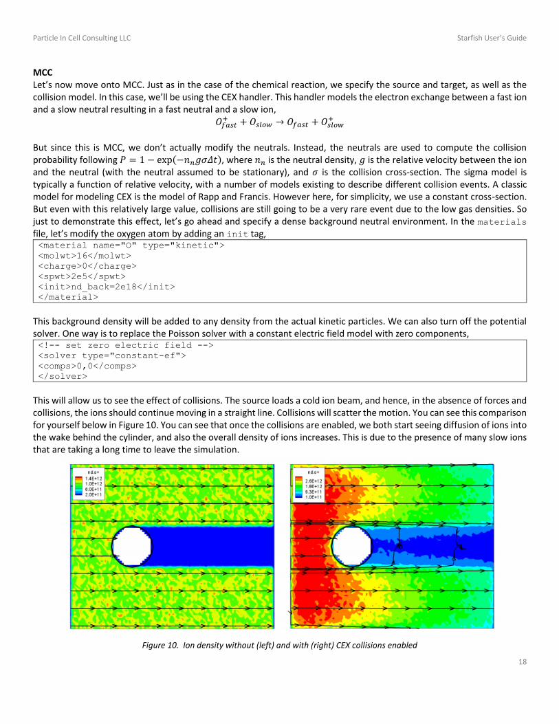
This will allow us to see the effect of collisions. The source loads a cold ion beam, and hence, in the absence of forces and collisions, the ions should continue moving in a straight line. Collisions will scatter the motion. You can see this comparison for yourself below in Figure 10. You can see that once the collisions are enabled, we both start seeing diffusion of ions into the wake behind the cylinder, and also the overall density of ions increases. This is due to the presence of many slow ions that are taking a long time to leave the simulation.
Figure 10. Ion density without (left) and with (right) CEX collisions enabled
Particle In Cell Consulting LLC Starfish User’s Guide
19
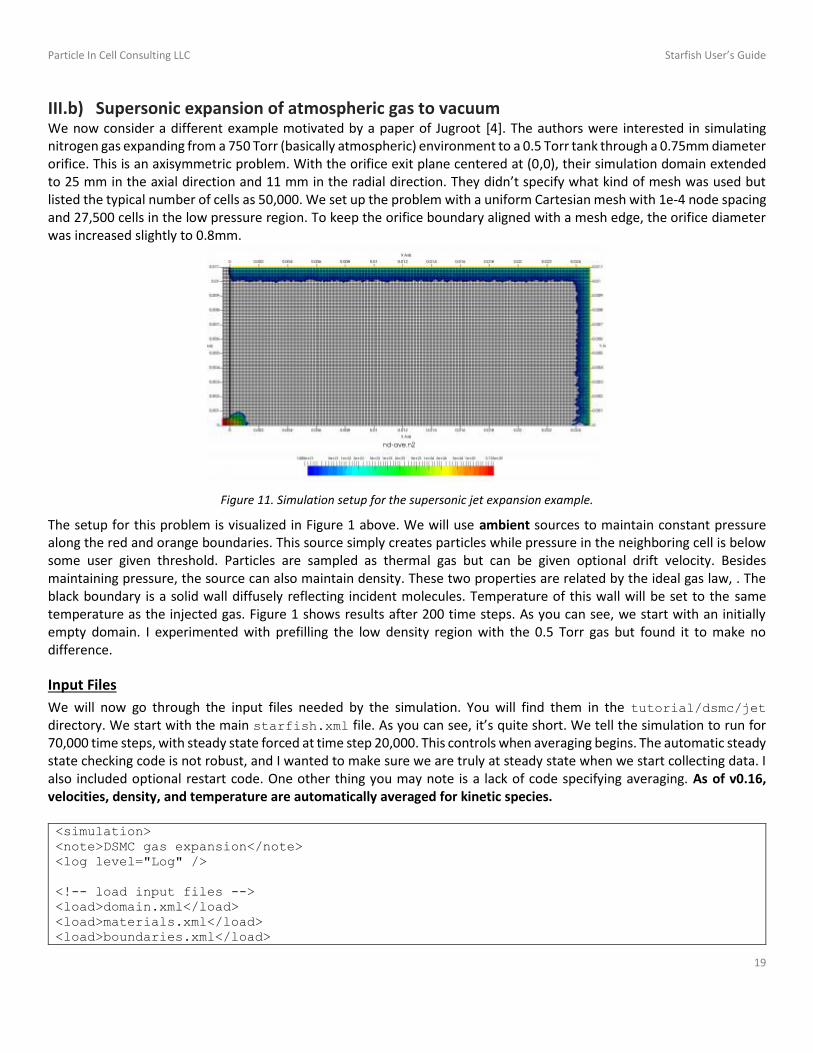
III.b) Supersonic expansion of atmospheric gas to vacuum We now consider a different example motivated by a paper of Jugroot [4]. The authors were interested in simulating nitrogen gas expanding from a 750 Torr (basically atmospheric) environment to a 0.5 Torr tank through a 0.75mm diameter orifice. This is an axisymmetric problem. With the orifice exit plane centered at (0,0), their simulation domain extended to 25 mm in the axial direction and 11 mm in the radial direction. They didn’t specify what kind of mesh was used but listed the typical number of cells as 50,000. We set up the problem with a uniform Cartesian mesh with 1e-4 node spacing and 27,500 cells in the low pressure region. To keep the orifice boundary aligned with a mesh edge, the orifice diameter was increased slightly to 0.8mm.
Figure 11. Simulation setup for the supersonic jet expansion example.
The setup for this problem is visualized in Figure 1 above. We will use ambient sources to maintain constant pressure along the red and orange boundaries. This source simply creates particles while pressure in the neighboring cell is below some user given threshold. Particles are sampled as thermal gas but can be given optional drift velocity. Besides maintaining pressure, the source can also maintain density. These two properties are related by the ideal gas law, . The black boundary is a solid wall diffusely reflecting incident molecules. Temperature of this wall will be set to the same temperature as the injected gas. Figure 1 shows results after 200 time steps. As you can see, we start with an initially empty domain. I experimented with prefilling the low density region with the 0.5 Torr gas but found it to make no difference.
Input Files
We will now go through the input files needed by the simulation. You will find them in the tutorial/dsmc/jet directory. We start with the main starfish.xml file. As you can see, it’s quite short. We tell the simulation to run for 70,000 time steps, with steady state forced at time step 20,000. This controls when averaging begins. The automatic steady state checking code is not robust, and I wanted to make sure we are truly at steady state when we start collecting data. I also included optional restart code. One other thing you may note is a lack of code specifying averaging. As of v0.16, velocities, density, and temperature are automatically averaged for kinetic species. <simulation>
<note>DSMC gas expansion</note>
<log level="Log" />
<!-- load input files -->
<load>domain.xml</load>
<load>materials.xml</load>
<load>boundaries.xml</load>

Particle In Cell Consulting LLC Starfish User’s Guide
20
<load>interactions.xml</load>
<load>sources.xml</load>
<!-- set time parameters -->
<time>
<num_it>70000</num_it>
<dt>1e-8</dt>
<steady_state>20000</steady_state>
</time>
<!-- run simulation -->
<starfish/>
<!-- save results -->
<output type="2D" file_name="field.vts" format="vtk">
<scalars>nodevol, p, nd-ave.n2, t.n2, t1.n2, t2.n2, t3.n2, nu, mpc.n2, dsmc-
count</scalars>
<vectors>u-ave.n2, v-ave.n2, w-ave.n2</vectors>
</output>
<output type="boundaries" file_name="boundaries.vtp" format="vtk">
<scalars>flux.n2, flux-normal.n2</scalars>
</output>
</simulation>
The variables that we are outputting include node volume, total pressure, average number density of nitrogen, total temperature, temperature components for the three spatial directions, average velocity components, collision rate, average number of macroparticles per cell, and average number of collisions per cell. All this data is saved as point data. In the future, I will make the output algorithm more user friendly by having it save velocity components directly as vectors. The domain.xml file specifies the uniform mesh used for particle push, collisions, and sampling: <domain type="zr">
<mesh type="uniform" name="mesh">
<origin>-5e-4,0</origin>
<spacing>1.0e-4, 1.0e-4</spacing>
<nodes>256, 111</nodes>
<mesh-bc wall="bottom" type="symmetry"/>
</mesh>
</domain>
It is not necessary to specify symmetry on 𝑟 = 0 the edge for an axisymmetric code (domain type="zr") but I left it here in case you want the run the code in the xy mode (domain type="xy") The materials.xml file lists known materials used for specifying boundaries and gas particles, <materials>
<material name="N2" type="kinetic">
<molwt>28</molwt>
<charge>0</charge>
<spwt>1e11</spwt>

Particle In Cell Consulting LLC Starfish User’s Guide
21
<ref_temp>275</ref_temp>;
<visc_temp_index>0.74</visc_temp_index>
<vss_alpha>1.00</vss_alpha> <!--1.36-->
<diam>4.17e-10</diam>
</material>
<material name="SS" type="solid">
<molwt>52.3</molwt>
<density>8000</density>
</material>
</materials>
The file lists two materials: nitrogen molecules and stainless steel for surfaces. One important thing to note here is that for a kinetic material (flying gas particles) we also specify various DSMC parameters. These values for nitrogen come from Tables A1, A2 and A3 in Appendix A of Bird’s 2003 book. The vss_alpha can be used to turn on the Variable Soft Sphere (VSS) collision model. Value of 1 results in the faster Variable Hard Sphere (VHS) being used. I ran few cases and did not observe any significant differences between the two and hence we’ll be using VHS in this example. You can speed up the code by using a higher specific weight with the risk of adding numerical error due to not having enough particles per cell. The boundaries.xml file specifies surface boundaries in an SVG format. You could generate the segments for complex geometries using “path to SVG” in GIMP or Inkscape, but for a simple geometry, you can just make the file by hand, <boundaries>
<boundary name="wall" type="solid">
<material>SS</material>
<path>M 0, 11e-3 L 0,8e-4 -1e-3,8e-4</path>
<temp>288</temp>
</boundary>
<boundary name="inlet" type="solid">
<material>SS</material>
<path>M wall:last L -1e-3,0</path>
<temp>288</temp>
</boundary>
<boundary name="ambient" type="virtual">
<path>M 25e-3,0 L 25e-3,11e-3 0,11e-3</path>
</boundary>
</boundaries>
The “ambient” boundary is marked as virtual. This allows this boundary to be used when specifying particle sources but is subsequently invisible to particles during the push. Although “inlet” is marked as solid, it doesn’t seem to make a difference. A virtual inlet means that a particle moving back to the tank is removed, and subsequently new particle is generated by the ambient source. However, since both use the same algorithm to sample a half Maxwellian, the result is the same. Particles sources are listed in the sources.xml file,

Particle In Cell Consulting LLC Starfish User’s Guide
22
<sources>
<!--high pressure tank-->
<boundary_source name="inlet_750Torr" type="ambient">
<enforce>pressure</enforce>
<material>N2</material>
<boundary>inlet</boundary>
<drift_velocity>0,0,0</drift_velocity>
<temperature>288</temperature>
<total_pressure>1.0e5</total_pressure>
</boundary_source>
<!--ambient environment-->
<boundary_source name="amb_0.5Torr" type="ambient">
<enforce>pressure</enforce>
<material>N2</material>
<boundary>ambient</boundary>
<drift_velocity>0,0,0</drift_velocity>
<temperature>288.0</temperature>
<total_pressure>66.66</total_pressure>
</boundary_source>
</sources>
As you can see, we are specifying two sources of type ambient. This source attempts to maintain constant density, pressure, or partial pressure (as given by the enforce parameter) in cells along the given boundary. Particles are sampled from a half-Maxwellian at the given temperature (288K). The first source generates particles for the 750 Torr reservoir, while the second source generates particles to fill the low pressure tank. Pressures are given in Pascal, hence values in Torr need to be multiplied by 133.322. Finally, we have interactions.xml file, which specifies particle-surface and particle-particle interactions, <material_interactions>
<surface_hit source="N2" target="SS">
<product>N2</product>
<model>diffuse</model>
<prob>1.0</prob>
</surface_hit>
<dsmc model="elastic">
<pair>N2,N2</pair>
<sigma>Bird463</sigma>
</dsmc>
</material_interactions>
This file tells the simulation that a nitrogen molecule hitting a stainless steel surface should reflect diffusely. Collisions between nitrogen molecules are handled with DSMC, with the collision cross-section given by Equation 4.63 in [3].
Results
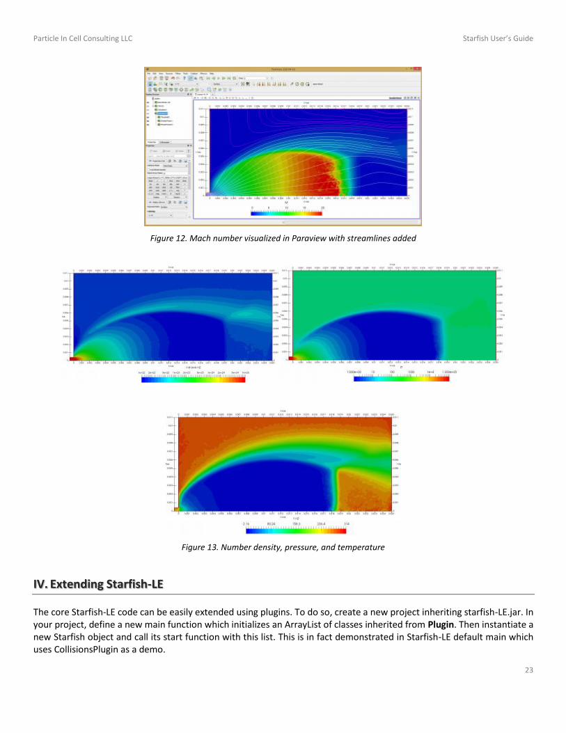
Once the simulation finishes, you will have a file called field.vts which you can visualize using Paraview, Figure 12 The online article discusses some steps for visualizing this file. Figure 13 shows the gas number density, pressure, and temperature. We can clearly see the formation of a the triple point and a Mach disc.
Particle In Cell Consulting LLC Starfish User’s Guide
23
Figure 12. Mach number visualized in Paraview with streamlines added
Figure 13. Number density, pressure, and temperature
IV. Extending Starfish-LE
The core Starfish-LE code can be easily extended using plugins. To do so, create a new project inheriting starfish-LE.jar. In your project, define a new main function which initializes an ArrayList of classes inherited from Plugin. Then instantiate a new Starfish object and call its start function with this list. This is in fact demonstrated in Starfish-LE default main which uses CollisionsPlugin as a demo.

Particle In Cell Consulting LLC Starfish User’s Guide
24
public static void main(String args[])
{
/*demo of starting Starfish with plugins*/
ArrayList<Plugin> plugins = new ArrayList<Plugin>();
plugins.add(new CollisionsPlugin());
/*make a new instance*/
new Starfish().start(args, plugins);
}
Each command that can be called from the XML input file corresponds to an object derived from RunnableModule. The code begins by registering known modules such as “time”, “starfish”, “output” and so on. Next, the register method is called on each provided plugin: /*register modules*/
RegisterModules();
if (plugins!=null)
for (Plugin plugin:plugins)
plugin.register();
Withing this register method you can add whatever code is needed to extend the code capabilities. For instance, the Collisions plugin registers additional interaction types and a collision cross-section as: public void register()
{
/*add new interactions*/
InteractionsModule.registerInteraction("DSMC",DSMC.DSMCFactory);
InteractionsModule.registerInteraction("MCC", MCC.MCCFactory);
/*add cross-section*/
InteractionsModule.registerSigma("Bird463",SigmaPlus.makeSigmaBird463);
}
Please do not hesitate to contact us for more specific information.
V. Bugs and Future Work
Please report any bugs or feature requests to [email protected]. Current work on Starfish includes the following: 1. Re-enabling of multi-mesh support 2. Addition of automatic adaptive mesh refinement 3. Improvements in parallelization by adding support to additional functions 4. Implementation of an electromagnetic EM-PIC model 5. Addition of fluid solver

Particle In Cell Consulting LLC Starfish User’s Guide
25
VI. Command Reference
This section summarizes all commands that can be included in the starfish.xml file. Each key can be supplied as an attribute or as an XML node, for instance <starfish randomize=”true”/> and <starfish> <randomize>true</randomize> </starfish> are identical. Examples of data field types are given below.
type description example(s)
int integer (whole number) value -1
int2 two integers separated by comma 41,50
float a floating point number in double precision 1.06e23
float2 two floats separated by comma 1.07,-3.2
float_list arbitrary number of comma-separated floats -23.2,0,12.8
bool a true or false value true
string any text inlet
string_list multiple comma separated strings pressure, nd.xe
string_pairs multiple comma separated strings in “s1=s2” format. The “s1=” part is not needed if “s2=s2”.
bfi=bi, sigma
string_tupples multiple pairs of strings grouped inside square brackets [u.xe,v.xe], [efi, efj]
element a valid child XML element <output> ... </output>
VI.a) General VI.a.1) NOTE
Prints the specified message to the screen and log file.
Key Type Default Description
N/A string Note body
Example <note>Simulation of ion flow past a charged sphere</note>
VI.a.2) LOG
Controls logging level
Key Type Default Description
level string One of [DEBUG, LOG_LOW, LOG, MESSAGE, WARNING, ERROR, EXCEPTION]. Error and exception messages get printed regardless of the log level.
Example

Particle In Cell Consulting LLC Starfish User’s Guide
26
<note>Simulation of ion flow past a charged sphere</note>
VI.a.3) RESTART
Controls saving and reloading of restart data. Currently only particle data are saved. Support for field and fluid materials saving and restarting is pending.
Key Type Default Description
it_save bool 500 Frequency of restart data saves
nt_add int -1 Number of additional time steps to run after restart load if >0
load bool false Controls whether restart file should be loaded
save bool false Controls whether restart data should be saved
Example <restart it_save="200" nt_add="2500" load="true" save="false" />
VI.a.4) STARFISH
Runs the actual simulation.
Key Type Default Description
randomize bool true Will randomize the random number generator if true. Set to false to replicate the same simulation.
max_processors int num CPUs -1 Maximum number of threads to use for multithreading. By default set to CPU “number of cores” minus 1.
Example <starfish randomize="true" />
VI.a.5) STOP
Stops the simulation. Used for debugging, as the rest of the input file will not processed. Otherwise, the rest of the commands would need to be commented out.
Key Type Default Description
Example
<stop />
VI.a.6) TIME
Controls the duration of the simulation.
Key Type Default Description
dt float Simulation time step, in seconds.
num_it int Number of time steps to simulate.
steady_state string / int
auto Time step at which the steady state is reached. If “auto”, Starfish automatically sets steady state based on differences in particle counts.
Example <time>

Particle In Cell Consulting LLC Starfish User’s Guide
27
<dt>5e-6</dt>
<num_it>1000</num_it>
</time>
VI.b) Input / Output
VI.b.1) ANIMATION
Wrapper to periodically save simulation results. Works by executing <output> at the specified interval.
Key Type Default Description
start_it int Time step at which output should begin
frequency int Number of time steps between file saves
output element Entire <output> XML element, following syntax as noted below. For VTK files, file name will be modified to include the time step number.
Example <animation start_it="1" frequency="50">
<output type="2D" file_name="results/field_ani.vts" format="vtk">
<scalars>phi, nd.xe+,nd.xe</scalars>
<vectors>[efi, efj], [u.xe+,v.xe+]</vectors>
</output>
</animation>
VI.b.2) AVERAGING
Enables averaging of specified variables. The averaged values will have “-ave” append to the prefix. For instance, the average number density of o+ will be called “nd-ave.o+”, while “nd.o+” will contain the instantons data. Starting time step should correspond to time after steady state is reached.
Key Type Default Description
frequency int 1 Number of time steps between averaging samples
start_it int -1 Starting time step for averaging
variables string_list List of variables to average
Example
<averaging frequency="25" start_it="10000">
<variables>phi,rho,nd.o+,nd.e-,u.o+,v.o+</variables>
</averaging>
VI.b.3) LOAD_FIELD
Loads field data from a file. Can be used, among other things, to load an external magnetic field.
Key Type Default Description
format string TECPLOT File format. By default, the code supports TECPLOT or TABLE. A TECPLOT file should list variables on a single VARIABLES line. The TABLE format is assumed to start with ni,nj, and is hardcoded for “z,r,B,Bz,Br” data.
file_name string name of the file to load

Particle In Cell Consulting LLC Starfish User’s Guide
28
coords string_list names of two file variables to correspond to XY, RZ, or ZR, according to the specified <domain> type.
vars string_pairs variables to load in “starfish_var=file_var” format. The assignment part is not needed if the file variable is the same as the expected Starfish variable name.
Example
<load_field format="tecplot" name="bfield">
<file_name>bfield.dat</file_name>
<coords>z,r</coords>
<vars>bfi=bz,bfj=br,lambda</vars>
</load_field>
-- example of a Tecplot file format –-
VARIABLES = "z", "r", "n_n"
ZONE I=52, J=18, F=POINT
0.0491 0.0071 1.09994e+014
-- example of a Table format --
47 22
-0.018 0 0.03 0.03 0
VI.b.4) OUTPUT
Wrapper to periodically save simulation results. Works by executing <output> at the specified interval.
Key Type Default Description
type string Type of output to generate. Must be one of “1D”, “2D”, “boundaries”, or “particles”.
file_name string Name of output file
format string Output file format. Currently only “TECPLOT” and “VTK” are supported.
scalars (or variables)
string_list List of node-centered scalar variables to output. For backward compatibility, “variables” can be used as well.
cell_data string_list List of cell-centered scalars to output
vectors string_tupples Pairs of node-centered scalar variables to group together as vectors. Only affects VTK output.
TYPE = “1D”
Saves a slice of mesh data by exporting data only along a single given “i” or “j” index.
mesh string Name of the mesh to output (only a single mesh output is supported).
index string Logical grid position to output in format “I=xx” or “J=xx”
TYPE = “2D”
Saves mesh field data. No additional inputs.
TYPE = “BOUNDARIES”

Particle In Cell Consulting LLC Starfish User’s Guide
29
Saves surface data along boundaries. No additional inputs.
TYPE = “PARTICLES”
Exports user specified number of randomly selected particles.
count int Number of particles to output
Example
<output type="1D" file_name="profile.vts" format="vtk">
<mesh>mesh1</mesh>
<index>I=1</index>
<variables>phi, rho, nd.xe+</variables>
</output>
<output type="2D" file_name="results/field.vts" format="vtk">
<scalars>psi, phi, te, rho, sigma, nd.xe+</scalars>
<vectors>[ue,ve], [u.xe+, v.xe+], [efi, efj], [jx,jy]</vectors>
</output>
<output type="boundaries" file_name="boundaries.vtp" format="vtk">
<variables>deprate.xe+, flux-normal.xe+</variables>
</output>
<output type="particles" file_name="particles.dat" format="tecplot">
<species>ti2+,e-</species>
<count>10000,10000</count>
</output>
VI.b.5) PARTICLE_TRACE
Command to sample position and velocity of a specified particle to generate a trace file
Key Type Default Description
file_name string Name of output file
format string TECPLOT File format, currently only “TECPLOT” and “VTK” are supported.
material string Material of the sampled particle
id int Particle id
start_it int Starting time step for output
Example
<particle_trace file_name="trace.dat" material="HC">
<id>20685</id>
<start_it>495</start_it>
</particle_trace>
VI.b.6) STATS
Command to control frequency of saves to a global diagnostics file
Key Type Default Description
Particle In Cell Consulting LLC Starfish User’s Guide
30
file_name string starfish_stats.csv Stats file name
skip int 1 Output frequency. Value <=0 disables file output.
Example
<stats skip="10" />
VI.c) Materials VI.c.1) MATERIALS
Definition of materials known to the simulation. Contains one or more <material> elements.
Key Type Default Description
material element Material definition. See the following entry for Material for data fields.
Example
<materials>
<material name="Ar" type="kinetic">
..
</material>
<material name="SS" type="solid">
..
</material>
</materials>
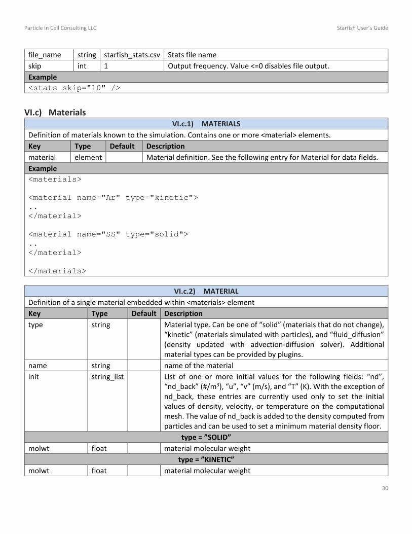
VI.c.2) MATERIAL
Definition of a single material embedded within <materials> element
Key Type Default Description
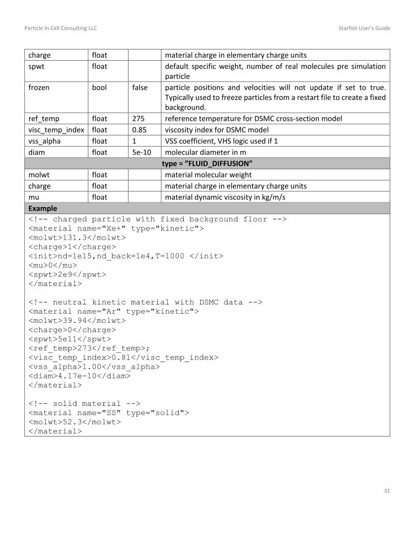
type string Material type. Can be one of “solid” (materials that do not change), “kinetic” (materials simulated with particles), and “fluid_diffusion” (density updated with advection-diffusion solver). Additional material types can be provided by plugins.
name string name of the material
init string_list List of one or more initial values for the following fields: “nd”, “nd_back” (#/m3), “u”, “v” (m/s), and “T” (K). With the exception of nd_back, these entries are currently used only to set the initial values of density, velocity, or temperature on the computational mesh. The value of nd_back is added to the density computed from particles and can be used to set a minimum material density floor.
type = ”SOLID”
molwt float material molecular weight
type = ”KINETIC”
molwt float material molecular weight
Particle In Cell Consulting LLC Starfish User’s Guide
31
charge float material charge in elementary charge units
spwt float default specific weight, number of real molecules pre simulation particle
frozen bool false particle positions and velocities will not update if set to true. Typically used to freeze particles from a restart file to create a fixed background.
ref_temp float 275 reference temperature for DSMC cross-section model
visc_temp_index float 0.85 viscosity index for DSMC model
vss_alpha float 1 VSS coefficient, VHS logic used if 1
diam float 5e-10 molecular diameter in m
type = ”FLUID_DIFFUSION”
molwt float material molecular weight
charge float material charge in elementary charge units
mu float material dynamic viscosity in kg/m/s
Example
<!-- charged particle with fixed background floor -->
<material name="Xe+" type="kinetic">
<molwt>131.3</molwt>
<charge>1</charge>
<init>nd=1e15,nd_back=1e4,T=1000 </init>
<mu>0</mu>
<spwt>2e9</spwt>
</material>
<!-- neutral kinetic material with DSMC data -->
<material name="Ar" type="kinetic">
<molwt>39.94</molwt>
<charge>0</charge>
<spwt>5e11</spwt>
<ref_temp>273</ref_temp>;
<visc_temp_index>0.81</visc_temp_index>
<vss_alpha>1.00</vss_alpha>
<diam>4.17e-10</diam>
</material>
<!-- solid material -->
<material name="SS" type="solid">
<molwt>52.3</molwt>
</material>

Particle In Cell Consulting LLC Starfish User’s Guide
32
VI.d) Material Interactions VI.d.1) MATERIAL_INTERACTIONS
Controls inter-material interactions, including the gas material / surface boundary interface. Interactions are specified via child elements. Starfish natively supports four types of interactions:
1. surface_hit: interaction between material and a surface boundary 2. dsmc: interaction between two kinetic materials 3. mcc: interaction between a kinetic source and a fluid target 4. chemistry: interaction between two fluid materials
Key Type Default Description
surface_hit / mcc / chemistry / dsmc
element Available interaction types. Additional types can be implemented by plugins.
Example
<material_interactions>
<surface_hit>
...
</surface_hit>
<dsmc>
...
</dsmc>
</material_interactions>
VI.d.2) SURFACE_HIT
Command to control frequency of saves to a global diagnostics file
Key Type Default Description
file_name string starfish_stats.csv Stats file name
skip int 1 Output frequency. Value <=0 disables file output.
Example
<stats skip="10" />
VI.d.3) DSMC
Enables DSMC collisions between two kinetic materials
Key Type Default Description
pair string_list Names of the two materials participating in this interaction
model string Currently only “elastic” is supported
frequency int 1
sig_cr_max float 1e-16
sigma string Collision cross-section. Natively the following models are supported:

Particle In Cell Consulting LLC Starfish User’s Guide
33
const: 𝜎 = 𝑐0
inv: 𝜎 = 𝑐0/𝑔
bird463: 𝜎 = 0.25𝜋𝑑𝑟𝑒𝑓2 (
2𝑘𝑇𝑟𝑒𝑓
𝑚𝑟𝑔2)𝜔−0.5
/Γ(2.5 − 𝜔) ,
equation 4.63 in Bird 2003
sigma_coeffs float_list Collision cross-section coefficients
Example
<dsmc model="elastic">
<pair>N2,N2</pair>
<sigma>Bird463</sigma>
</dsmc>
VI.d.4) MCC
Enables MCC collisions between a kinetic and fluid / kinetic target. Properties of the target material are not affected by the collision and hence this interaction is suitable only for cases of a rarefied source material interacting with a much denser target. A kinetic material can be used as the target, in which case, the density obtained by scattering particles to the grid will be used to obtain collision probability.
Key Type Default Description
source string Name of the source kinetic material.
target string Name of the target fluid or kinetic material
product <source> Optional post-collision material of the source. By default, there is no species change.
model Collsion model. Can be “MEX” / “ELASTIC” for momentum transfer, or “CEX” for charge exchange collision
sigma string Collision cross-section. See description of DSMC for details.
sigma_coeffs float_list Collision cross-section coefficients.
Example
<mcc model="cex">
<target>ar</target>
<source>ar+</source>
<sigma>inv</sigma>
<sigma_coeffs>1e-16</sigma_coeffs>
</mcc>
VI.d.5) CHEMISTRY
Enables fluid-fluid interactions. Densities of source materials (which can be kinetic or fluid) along with temperature (or energy) of a dependent material are used to compute the reaction, 𝑛𝑠1𝑛𝑠2𝑘(𝑇𝑑). Products are then generated accordingly and source material densities are depleted.
Key Type Default Description
sources string_list List of reactants with optional multipliers
products string_list List of products

Particle In Cell Consulting LLC Starfish User’s Guide
34
rate element Reaction rate equation type
RATE
type string Currently only “POLYNOMIAL” is supported. This evaluates (𝑐0 + 𝑐1𝑣 +𝑐2𝑣
2 + ⋯)𝑐𝑚𝑢𝑙𝑡
coeffs float_list List of model coefficients
multiplier float Coefficient multiplier
dep_var element Information about the dependent variable 𝑣 in the rate model.
DEP_VAR
mat string name of the dependent variable
wrapper string NONE Options are NONE, LOG10, or LOG10ENERGY
Example
<chemistry>
<sources>Xe,e-</sources>
<products>Xe+,2*e-</products>
<rate type="polynomial">
<coeffs>-0.57, 6.1978, -23.19, 30.439, 2.8407, -18.722</coeffs>
<multiplier>1e-20</multiplier>
<dep_var wrapper="log10energy" mat="e-" />
</rate>
</chemistry>
VI.e) Boundaries VI.e.1) BOUNDARIES
This command is used to define the surface geometry. It contains several <boundary> elements each specifying a particular surface spline.
Key Type Default Description
boundary element Definition of a single boundary
transform element Optional, defines global transformation applied to all boundaries
TRANSFORM
scaling float2 1,1 Scaling in the i and j direction
translation float2 0,0 translation in the I and j direction
rotation float 0 Rotation about the z axis
reverse bool false Flips normal vector orientation
Example
<boundaries>
<transform>
<scaling>1e-3,-1e-3</scaling>
<translation>0,0</translation>
<reverse>true</reverse>
</transform>

Particle In Cell Consulting LLC Starfish User’s Guide
35
<boundary>...</boundary>
<boundary>...</boundary>
</boundaries>
VI.e.2) BOUNDARY
Defines a single surface boundary spline.
Key Type Default Description
name string Name of the boundary
type string solid Boundary type. Can be one of: SOLID for a solid surface with fixed Dirchlet b.c., OPEN for Neumann b.c. (not fully supported), SYMMETRY for symmetric boundary reflecting particles, VIRTUAL for boundaries useful for attaching sources but that are not affect material propagation, and SINK for an absorbing boundary. Note that some of these are either extraneous or not yet fully implemented.
value float 0 Boundary condition value. For SOLID boundaries this sets the Dirichlet potential for the Poisson solver.
material string Boundary material, only required for SOLID
temp float 273.15 Boundary temperature, used to compute post-impact velocity
path string Spline definition in SVG-like format. The general syntax is [COMMAND] x1,y1 x2,y2 ... [COMMAND] x,y. The following commands are supported: “M x,y” move to (x,y), “m dx,dy” move by offset (dx,dy), “L x,y” line to (x,y) from the previous point, “l dx,dy” line to point offset by (dx,dy) from the last point, “C x1,y1 x2,y2,...” smooth cubic spline through points (x1,y1), (x2,y2), ... Commands do not need to be repeated, for instance “M x1,y1 L x2,y2 L x3,y3 L x4,y4” can be written as “M x1,y1 L x2,y2 x3,y3 x4,y4”. Points need to be specified in counter-clockwise order around an solid boundary (or in clockwise order around an open boundary), as point ordering controls the normal vector orientation. Note that unlike in SVG, cubic splines are specified by simply listing the points through which the spline will pass and the control knot points are omitted.
transform element Optional transformation parameters
reverse bool Optional, flips normal vector orientation, overridden by entry in <transform> if both defined.
Example
<boundary name="inlet" value="300">
<material>SS</material>
<path>M 0,0 L 400,71</path>
<material>vent</material>
<reverse>true</reverse>
<transform>
<scaling>1e-3,1e-3</scaling>
</transform>
</boundary>
Particle In Cell Consulting LLC Starfish User’s Guide
36
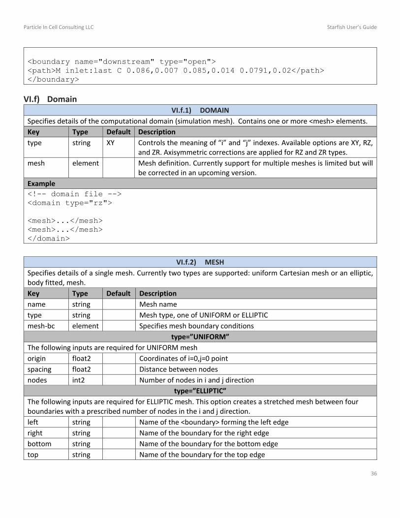
<boundary name="downstream" type="open">
<path>M inlet:last C 0.086,0.007 0.085,0.014 0.0791,0.02</path>
</boundary>
VI.f) Domain VI.f.1) DOMAIN
Specifies details of the computational domain (simulation mesh). Contains one or more <mesh> elements.
Key Type Default Description
type string XY Controls the meaning of “i” and “j” indexes. Available options are XY, RZ, and ZR. Axisymmetric corrections are applied for RZ and ZR types.
mesh element Mesh definition. Currently support for multiple meshes is limited but will be corrected in an upcoming version.
Example
<!-- domain file -->
<domain type="rz">
<mesh>...</mesh>
<mesh>...</mesh>
</domain>
VI.f.2) MESH
Specifies details of a single mesh. Currently two types are supported: uniform Cartesian mesh or an elliptic, body fitted, mesh.
Key Type Default Description
name string Mesh name
type string Mesh type, one of UNIFORM or ELLIPTIC
mesh-bc element Specifies mesh boundary conditions
type=”UNIFORM”
The following inputs are required for UNIFORM mesh
origin float2 Coordinates of i=0,j=0 point
spacing float2 Distance between nodes
nodes int2 Number of nodes in i and j direction
type=”ELLIPTIC”
The following inputs are required for ELLIPTIC mesh. This option creates a stretched mesh between four boundaries with a prescribed number of nodes in the i and j direction.
left string Name of the <boundary> forming the left edge
right string Name of the boundary for the right edge
bottom string Name of the boundary for the bottom edge
top string Name of the boundary for the top edge

Particle In Cell Consulting LLC Starfish User’s Guide
37
nodes int2 Number of nodes in i and j direction
MESH-BC
value float 0 Boundary condition value. Currently only used to set Dirichlet boundaries.
wall string Mesh wall to apply this boundary to. One of “left”, “right”, “bottom”, or “top”.
type string Mesh boundary type, supported values include OPEN, DIRICHLET< NEUMANN, PERIODIC, SYMMETRY, SINK, and CIRCUIT.
Example
<mesh type="uniform" name="mesh">
<origin>0, 0</origin>
<spacing>5e-5, 1e-4</spacing>
<nodes>51, 361</nodes>
<mesh-bc wall="left" type="symmetry" />
<mesh-bc wall="bottom" type="neumann" />
</mesh>
<mesh type="elliptic" name="downstream">
<left>exit_plane</left>
<bottom>symmetry_outside</bottom>
<right>downstream</right>
<top>body</top>
<nodes>35,13</nodes>
</mesh>
VI.g) Sources VI.g.1) SOURCES
Specifies material sources. Starfish supports two types of sources: boundary sources that inject mass along a specified boundary, and volume source that generate mass within the computational mesh.
Key Type Default Description
boundary_source / material_source / volume_source
element The actual source definitions
Example
<sources>
<boundary_source>...</boundary_source>
<volume_source>...</volume_source>
</sources>
VI.g.2) BOUNDARY_SOURCE
Specifies material sources. Starfish supports three types of sources: boundary that inject mass along a specified boundary, material sources that act like boundary sources but are applied to all boundaries with the given material, and volume source that generate mass within the computational mesh.

Particle In Cell Consulting LLC Starfish User’s Guide
38
Key Type Default Description
name string source name
type string source type, one of UNIFORM, MAXWELLIAN, AMBIENT, and COSINE
material string name of the injected material
boundary string surface boundary name to attach the source to
type=”UNIFORM”
This source injects a cold beam. It is a streamlined implementation of a Maxwellian source with T=0K.
mdot float Mass flow rate in kg/s
v_drift float Drift velocity in m/s
type=”MAXWELIAN”
Source for injecting mass sampled from the drifting Maxwellian velocity distribution function
mdot float Mass flow rate in kg/s
v_drift float Drift velocity in m/s
temperature float Temperature in K
start_it float 0 Time step to begin injection
end_it float -1 Time step to end injection, or -1 to ignore
type=”AMBIENT”
Generates mass in cells adjacent to the specified boundary such that prescribed density or pressure is maintained. Particle velocities are sampled from the Maxwellian distribution.
drift_velocity float3 0,0,0 Drift velocity to apply to sampled material
temperature float Assumed gas temperature in K, controls injection velocity and also used to scale pressure to density from 𝑃 = 𝑛𝑘𝑇.
enforce string TOTAL_PRESSURE Controls which property the source should maintain. Available options are TOTAL_PRESSURE, PARTIAL_PRESSURE, and DENSITY
density float Required for enforce=”DENSITY”, controls the desired number density in m-3.
total_pressure float Required for enforce=”TOTAL_PRESSURE” or “PARTIAL_PRESSURE”, in Pa
partial_pressure float Required for enforce=”PARTIAL_PRESSURE”, used to control the desired species fraction per 𝑃𝑖/𝑃𝑡𝑜𝑡
type=”COSINE”
Injects particles with velocity sampled from the cosine distribution about the surface normal
mdot float Injection mass flow rate in kg/s
v_drift float Drift velocity in m/s
Example
<boundary_source name="neutral_source" type="maxwellian">
<material>xe</material>
<boundary>inlet</boundary>
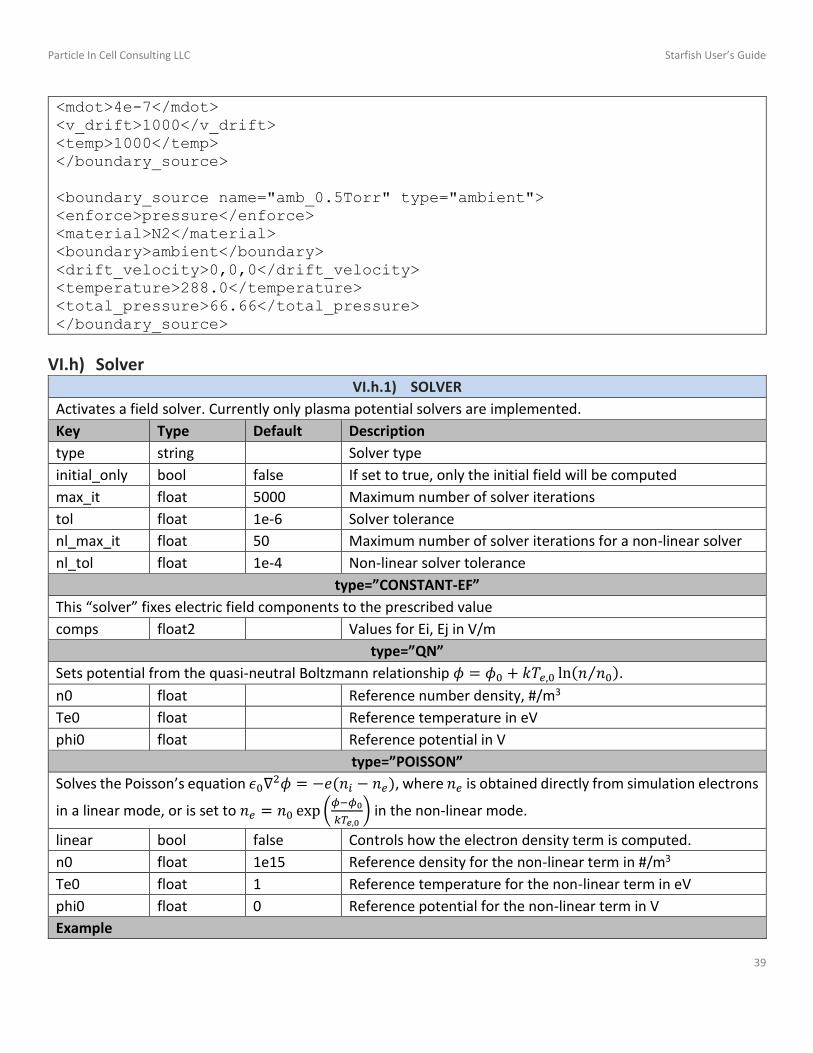
Particle In Cell Consulting LLC Starfish User’s Guide
39
<mdot>4e-7</mdot>
<v_drift>1000</v_drift>
<temp>1000</temp>
</boundary_source>
<boundary_source name="amb_0.5Torr" type="ambient">
<enforce>pressure</enforce>
<material>N2</material>
<boundary>ambient</boundary>
<drift_velocity>0,0,0</drift_velocity>
<temperature>288.0</temperature>
<total_pressure>66.66</total_pressure>
</boundary_source>
VI.h) Solver VI.h.1) SOLVER
Activates a field solver. Currently only plasma potential solvers are implemented.
Key Type Default Description
type string Solver type
initial_only bool false If set to true, only the initial field will be computed
max_it float 5000 Maximum number of solver iterations
tol float 1e-6 Solver tolerance
nl_max_it float 50 Maximum number of solver iterations for a non-linear solver
nl_tol float 1e-4 Non-linear solver tolerance
type=”CONSTANT-EF”
This “solver” fixes electric field components to the prescribed value
comps float2 Values for Ei, Ej in V/m
type=”QN”
Sets potential from the quasi-neutral Boltzmann relationship 𝜙 = 𝜙0 + 𝑘𝑇𝑒,0 ln(𝑛 𝑛0⁄ ).
n0 float Reference number density, #/m3
Te0 float Reference temperature in eV
phi0 float Reference potential in V
type=”POISSON”
Solves the Poisson’s equation 𝜖0∇2𝜙 = −𝑒(𝑛𝑖 − 𝑛𝑒), where 𝑛𝑒 is obtained directly from simulation electrons
in a linear mode, or is set to 𝑛𝑒 = 𝑛0 exp (𝜙−𝜙0
𝑘𝑇𝑒,0) in the non-linear mode.
linear bool false Controls how the electron density term is computed.
n0 float 1e15 Reference density for the non-linear term in #/m3
Te0 float 1 Reference temperature for the non-linear term in eV
phi0 float 0 Reference potential for the non-linear term in V
Example

Particle In Cell Consulting LLC Starfish User’s Guide
40
<!-- non-linear poisson solver example -->
<solver type="poisson">
<n0>1e12</n0>
<Te0>1.5</Te0>
<phi0>0</phi0>
<max_it>100000</max_it>
<tol>1e-3</tol>
<nl_tol>1e-2</nl_tol>
</solver>
<!-- prescribed electric field example -->
<solver type="constant-ef">
<comps>0,0</comps>
</solver>
<!-- quasineutral Boltzmann inversion example -->
<solver type="qn">
<n0>1e12</n0>
<Te0>1.5</Te0>
<phi0>0</phi0>
</solver>
VII. Data Fields
The below table summarizes data field and boundary variables in the baseline configuration. All material-specific fields follow syntax “base.mat”, for instance “nd.xe” is the number density of material “xe”. Averaged fields generated by the <averaging> command will have “-ave” appended to the base, for instance “phi-ave” and “nd-ave.xe”.
VII.a) Mesh Data
Name Units Description
VII.a.1) General
nodevol m-3 Mesh node volume, used for computing number density
phi V plasma potential
rho C/m3 charge density
efi,efj V/m electric field components
bfi,bfj T magnetic field components
p Pa total pressure
VII.a.2) Material-Specific (base.mat)
nd #/m3 material number density
u,v,w m/s node-averaged gas mean velocity
nd-ave #/m3 steady-state averaged number density

Particle In Cell Consulting LLC Starfish User’s Guide
41
u-ave,v-ave,w-ave m/s steady-state averaged gas mean velocity
t K average gas temperature
p Pa gas pressure, obtained from the ideal gas law
t1,t2,t3 K gas temperature in i,j,k direction
mpc # number of simulation macroparticles per cell
count-sum # internal variable used to obtain density, contains specific weight sum
u-sum,v-sum,w-sum m/s internal variable used to obtain velocity, contains sum of wspu
uu-sum,vv-sum,ww-sum
internal variable used to obtain temperature, contains sum of wspu2
mpc-sum # internal variable used to obtain mpc, contains sum of macroparticles
VII.a.3) MCC
mcc-count, mcc-count2, ...
# Number of collisions
mcc-nu, mcc-nu2, ... #/s Collision rate
mcc-real-sum, mcc-real-sum2, ...
# Internal variable used to compute MCC collision count, stores cumulative number of real particles undergoing collisions
mcc-count-sum, mcc-count-sum2, ...
# Internal variable used to compute MCC collision count, stores cumulative number of MCC collisions
VII.a.4) DSMC
dsmc-count, dsmc-count2, ...
# Number of collisions
nu, nu2 #/s Collision rate
dsmc-real-sum, dsmc-real-sum2, ...
# Internal variable used to compute DSMC collision count, stores cumulative number of real particles undergoing collisions
dsmc-count-sum, dsmc-count-sum2, ...
# Internal variable used to compute DSMC collision count, stores cumulative number of MCC collisions
VII.b) Boundary Data
Name Units Description
VII.b.1) Material-Specific
flux #/m2/s Total number of particles hitting the boundary per second, scaled by boundary area
flux-normal #/m2/s Particle flux multiplied by the cosine angle between the incoming velocity vector and surface normal
deprate kg/s Rate of mass depositing to the surface
depflux kg/m2/s Deposition rate scaled by the boundary area

Particle In Cell Consulting LLC Starfish User’s Guide
42
VIII. References
[1] L. Brieda and M. Keidar, "Development of the Starfish Plasma SImulation Code and Update on Multiscale Modeling of Hall Thrusters," in AIAA Joint Propulsion Conference, Atlanta, GA, 2012.
[2] C. Birdsall and A. Langdon, Plasma physics via Computer Simulations, Institute of Physics Publishing, 2000.
[3] G. Bird, Molecular Gas Dynamics and the Direct Simulation of Gas Flows, Oxford Science Publications, 1994.
[4] M. Jugroot, C. Groth, T. B, B. V and B. Collings, " Numerical investigation of interface region flows in mass spectrometers: neutral gas transport," J. of Phys., D: Applied Physics, vol. 37, pp. 1289-1300, 2004.