Stagnation Traps - CREI · Review of Economic Studies (2017) 01, 1{480034-6527/17/00000001$02.00 c...
48
Review of Economic Studies (2017) 01, 1–48 0034-6527/17/00000001$02.00 c 2017 The Review of Economic Studies Limited Stagnation Traps GIANLUCA BENIGNO London School of Economics, CEPR and CFM LUCA FORNARO CREI, Universitat Pompeu Fabra, Barcelona GSE and CEPR First version received XXX; final version accepted XXX (Eds.) We provide a Keynesian growth theory in which pessimistic expectations can lead to very persistent, or even permanent, slumps characterized by high unemployment and weak growth. We refer to these episodes as stagnation traps, because they consist in the joint occurrence of a liquidity and a growth trap. In a stagnation trap, the central bank is unable to restore full employment because weak growth depresses aggregate demand and pushes the policy rate against the zero lower bound, while growth is weak because low aggregate demand results in low profits, limiting firms’ investment in innovation. Aggressive policies aiming at restoring growth, such as subsidies to investment, can successfully lead the economy out of a stagnation trap by generating a regime shift in agents’ growth expectations. E32, E43, E52, O31, O42. 1. INTRODUCTION Can insufficient aggregate demand lead to economic stagnation, i.e. a protracted period of high unemployment and low growth? Economists have been concerned with this question at least since the Great Depression, 1 but interest in this topic has recently reemerged motivated by the two decades-long slump affecting Japan since the early 1990s, as well as by the slow recoveries experienced by the US and the Euro area in the aftermath of the 2008 financial crisis. In fact, all these long-lasting slump episodes have been characterized by the typical symptoms of liquidity traps: high unemployment, low real interest rates and nominal policy rates close to their zero lower bound (Table 1). Moreover, these episodes have been marked by slowdowns in investment, including investment in productivity enhancing activities such as R&D, 2 resulting in weak labor productivity growth and in large deviations of output from pre-slump trends (Figure 1). In this paper we present a theory in which very persistent, or even permanent, slumps characterized by high unemployment and low growth are possible. Our idea is that the connection between depressed demand, high unemployment and weak growth, far from being casual, can be the result of a two-way interaction. On the one hand, unemployment and weak aggregate demand can have a negative impact on firms’ 1. See Hansen (1939) for an early discussion of the relationship between aggregate demand, unemployment and technical progress. 2. As shown in Table 1, all the three slump episodes exhibit a fall in R&D intensity, defined as the ratio of investment in R&D to the R&D stock. As discussed in chapter 10 of Barro and Sala-i Martin (2004), R&D intensity is the key determinant of productivity growth in the seminal frameworks developed by Aghion and Howitt (1992), Grossman and Helpman (1991) and Romer (1990), as well as in the model that we present below. Kung and Schmid (2015) provide empirical evidence on the link between R&D intensity and productivity growth. Using US data for the period 1953-2008, these authors show that R&D intensity predicts productivity, output and consumption growth at horizons of one to five years. 1
Transcript of Stagnation Traps - CREI · Review of Economic Studies (2017) 01, 1{480034-6527/17/00000001$02.00 c...
Review of Economic Studies (2017) 01, 1–48 0034-6527/17/00000001$02.00
c© 2017 The Review of Economic Studies Limited
Stagnation Traps
GIANLUCA BENIGNO
London School of Economics, CEPR and CFM
LUCA FORNARO
CREI, Universitat Pompeu Fabra, Barcelona GSE and CEPR
First version received XXX; final version accepted XXX (Eds.)
We provide a Keynesian growth theory in which pessimistic expectations can leadto very persistent, or even permanent, slumps characterized by high unemployment andweak growth. We refer to these episodes as stagnation traps, because they consist in thejoint occurrence of a liquidity and a growth trap. In a stagnation trap, the central bankis unable to restore full employment because weak growth depresses aggregate demandand pushes the policy rate against the zero lower bound, while growth is weak because lowaggregate demand results in low profits, limiting firms’ investment in innovation. Aggressivepolicies aiming at restoring growth, such as subsidies to investment, can successfully leadthe economy out of a stagnation trap by generating a regime shift in agents’ growthexpectations.
E32, E43, E52, O31, O42.
1. INTRODUCTION
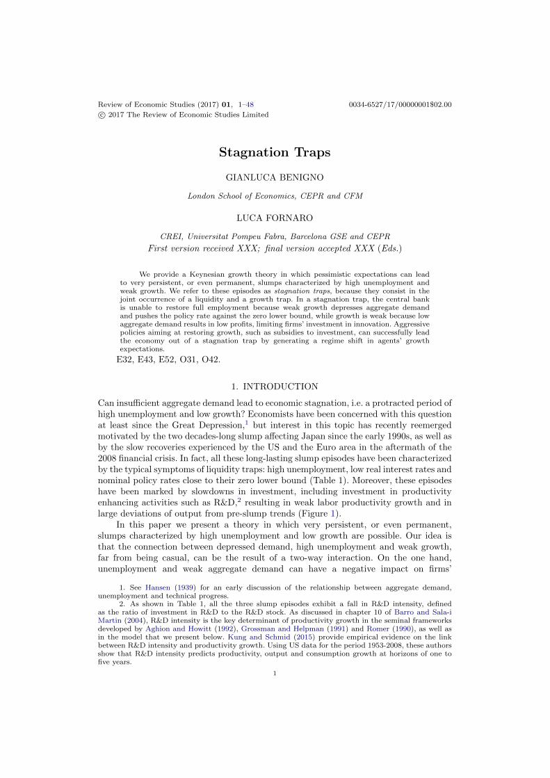
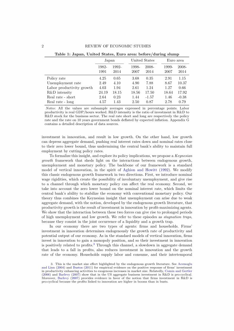
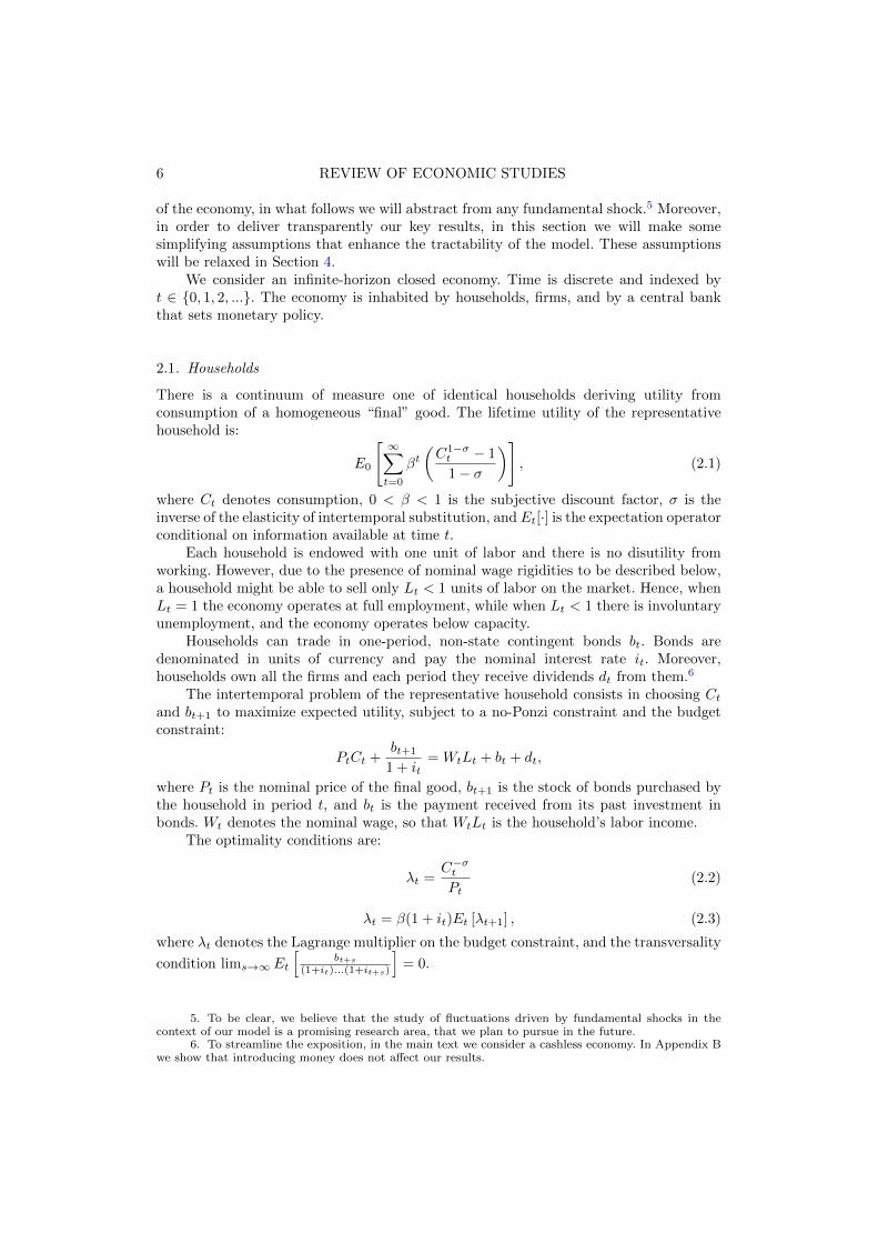
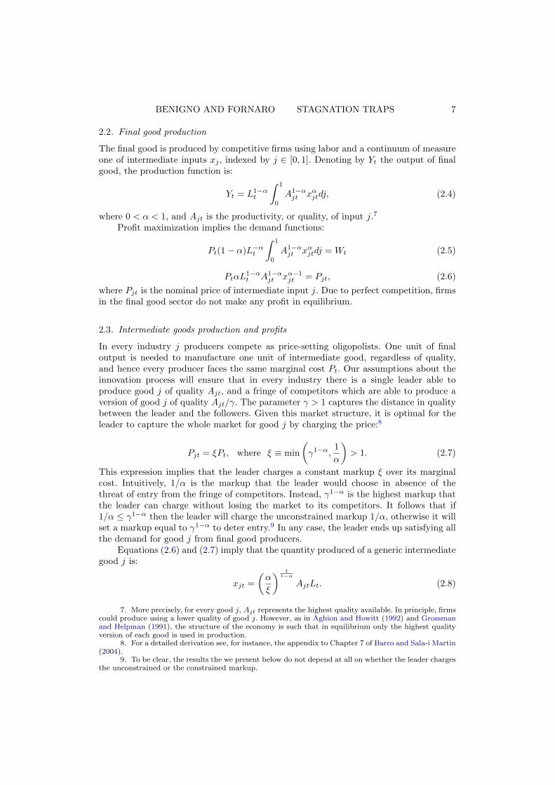
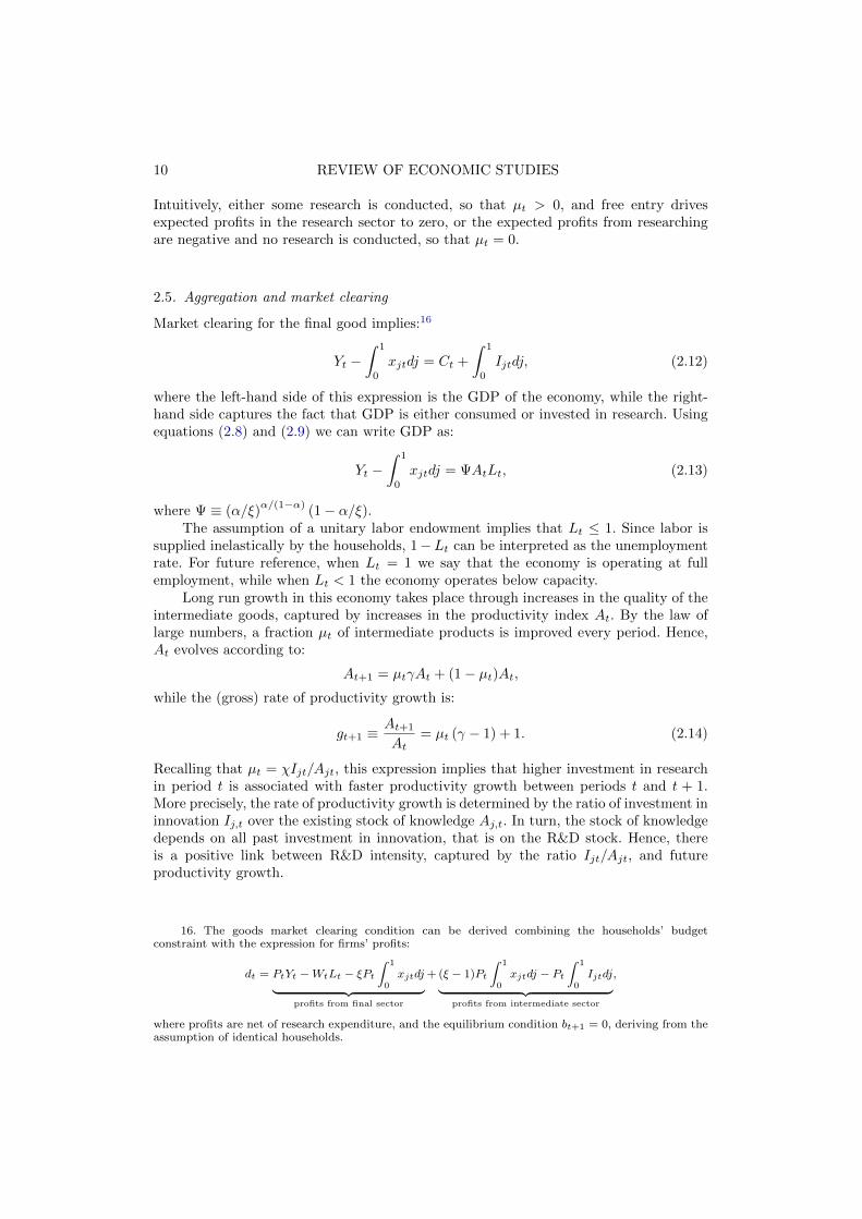
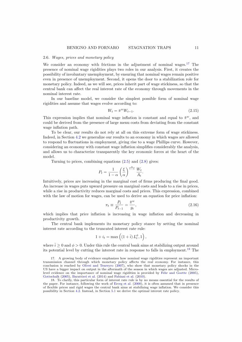
Can insufficient aggregate demand lead to economic stagnation, i.e. a protracted period ofhigh unemployment and low growth? Economists have been concerned with this questionat least since the Great Depression,1 but interest in this topic has recently reemergedmotivated by the two decades-long slump affecting Japan since the early 1990s, as well asby the slow recoveries experienced by the US and the Euro area in the aftermath of the2008 financial crisis. In fact, all these long-lasting slump episodes have been characterizedby the typical symptoms of liquidity traps: high unemployment, low real interest rates andnominal policy rates close to their zero lower bound (Table 1). Moreover, these episodeshave been marked by slowdowns in investment, including investment in productivityenhancing activities such as R&D,2 resulting in weak labor productivity growth and inlarge deviations of output from pre-slump trends (Figure 1).
In this paper we present a theory in which very persistent, or even permanent,slumps characterized by high unemployment and low growth are possible. Our idea isthat the connection between depressed demand, high unemployment and weak growth,far from being casual, can be the result of a two-way interaction. On the one hand,unemployment and weak aggregate demand can have a negative impact on firms’
1. See Hansen (1939) for an early discussion of the relationship between aggregate demand,unemployment and technical progress.
2. As shown in Table 1, all the three slump episodes exhibit a fall in R&D intensity, definedas the ratio of investment in R&D to the R&D stock. As discussed in chapter 10 of Barro and Sala-iMartin (2004), R&D intensity is the key determinant of productivity growth in the seminal frameworksdeveloped by Aghion and Howitt (1992), Grossman and Helpman (1991) and Romer (1990), as well asin the model that we present below. Kung and Schmid (2015) provide empirical evidence on the linkbetween R&D intensity and productivity growth. Using US data for the period 1953-2008, these authorsshow that R&D intensity predicts productivity, output and consumption growth at horizons of one tofive years.
1
2 REVIEW OF ECONOMIC STUDIES
Table 1: Japan, United States, Euro area: before/during slump
Japan United States Euro area
1982- 1992- 1998- 2008- 1999- 2008-1991 2014 2007 2014 2007 2014
Policy rate 4.25 0.65 3.68 0.35 2.91 1.15Unemployment rate 2.49 4.10 4.90 7.88 8.67 10.37Labor productivity growth 4.03 1.94 2.61 1.24 1.27 0.66R&D intensity 24.19 18.15 18.56 17.50 18.64 17.92Real rate - short 2.64 0.23 1.44 -1.57 1.46 -0.38Real rate - long 4.57 1.43 2.50 0.87 2.78 0.79
Notes: All the values are subsample averages expressed in percentage points. Laborproductivity is real GDP/hours worked. R&D intensity is the ratio of investment in R&D toR&D stock for the business sector. The real rate short and long are respectively the policyrate and the rate on 10 years government bonds deflated by expected inflation. Appendix Gcontains a detailed description of data sources.
investment in innovation, and result in low growth. On the other hand, low growthcan depress aggregate demand, pushing real interest rates down and nominal rates closeto their zero lower bound, thus undermining the central bank’s ability to maintain fullemployment by cutting policy rates.
To formalize this insight, and explore its policy implications, we propose a Keynesiangrowth framework that sheds light on the interactions between endogenous growth,unemployment and monetary policy. The backbone of our framework is a standardmodel of vertical innovation, in the spirit of Aghion and Howitt (1992). We modifythis classic endogenous growth framework in two directions. First, we introduce nominalwage rigidities, which create the possibility of involuntary unemployment, and give riseto a channel through which monetary policy can affect the real economy. Second, wetake into account the zero lower bound on the nominal interest rate, which limits thecentral bank’s ability to stabilize the economy with conventional monetary policy. Ourtheory thus combines the Keynesian insight that unemployment can arise due to weakaggregate demand, with the notion, developed by the endogenous growth literature, thatproductivity growth is the result of investment in innovation by profit-maximizing agents.We show that the interaction between these two forces can give rise to prolonged periodsof high unemployment and low growth. We refer to these episodes as stagnation traps,because they consist in the joint occurrence of a liquidity and a growth trap.
In our economy there are two types of agents: firms and households. Firms’investment in innovation determines endogenously the growth rate of productivity andpotential output of our economy. As in the standard models of vertical innovation, firmsinvest in innovation to gain a monopoly position, and so their investment in innovationis positively related to profits.3 Through this channel, a slowdown in aggregate demandthat leads to a fall in profits, also reduces investment in innovation and the growthrate of the economy. Households supply labor and consume, and their intertemporal
3. This is the market size effect highlighted by the endogenous growth literature. See Acemogluand Linn (2004) and Bustos (2011) for empirical evidence on the positive response of firms’ investmentin productivity enhancing activities to exogenous increases in market size. Relatedly, Comin and Gertler(2006) and Barlevy (2007) show that in the US aggregate business investment in R&D is pro-cyclical.Moreover, Barlevy (2007) provides evidence in favor of the notion that firms investment in R&D ispro-cyclical because the profits linked to innovation are higher in booms than in busts.
BENIGNO AND FORNARO STAGNATION TRAPS 3
1990 2000 2010
−0.2
0
0.2
0.4
Japan
2000 2005 2010
−0.15
−0.1
−0.05
0
0.05
0.1
United States
2000 2005 2010
−0.1
−0.05
0
0.05
0.1
Euro area
Figure 1Real GDP per capita
Notes: Series shown in logs, undetrended, centered around 1991 for Japan, and 2007 for United Statesand Euro area. Gross domestic product, constant prices, from IMF World Economic Outlook, dividedby total population from World Bank World Development Indicators. The linear trend is computed overthe period 1982-1991 for Japan, and 1998-2007 for United States and Euro area.
consumption pattern is characterized by the traditional Euler equation. The key aspectis that households’ current demand for consumption is affected by the growth rate ofpotential output, because productivity growth is one of the determinants of households’future income. In particular, a fall in the expected growth rate of potential output isassociated with lower future income and a reduction in current aggregate demand.4
This two-way interaction between productivity growth and aggregate demand resultsin two steady states. First, there is a full employment steady state, in which the economyoperates at potential and productivity growth is robust. However, our economy can alsofind itself in an unemployment steady state. In the unemployment steady state aggregatedemand and firms’ profits are low, resulting in low investment in innovation and weakproductivity growth. Moreover, monetary policy is not able to bring the economy at fullemployment, because the low growth of potential output pushes the interest rate againstits zero lower bound. Hence, the unemployment steady state can be thought of as astagnation trap.
Expectations, or animal spirits, are crucial in determining which equilibrium willbe selected. For instance, when agents expect growth to be low, expectations of lowfuture income reduce aggregate demand, lowering firms’ profits and their investment,thus validating the low growth expectations. Through this mechanism, pessimisticexpectations can generate a permanent liquidity trap with involuntary unemploymentand stagnation. We also show that, aside from permanent traps, pessimistic expectationscan give rise to stagnation traps of finite, but arbitrarily long, expected duration. Thisdoes not mean, however, that the fundamentals of the economy are unimportant. Infact, we find that expectations-driven permanent stagnation traps can arise only iffundamentals are such that the real interest rate in the full employment steady stateis low enough. This result suggests that structural factors that put downward pressureon the real interest rate, such as population aging, might also expose the economy to therisk of self-fulfilling stagnation traps.
4. Blanchard et al. (2017) provide evidence on the link between expectations of future productivitygrowth and current aggregate demand. Using US data for the period 1991-2014, they show that downwardrevisions in forecasts of future productivity growth are associated with unexpected falls in consumptionand investment.

4 REVIEW OF ECONOMIC STUDIES
In the last part of the paper, we derive some policy implications. We start by provingthat stagnation traps can take place even when monetary policy is conducted optimally.First, we show that a central bank operating under commitment can design interest raterules that eliminate the possibility of expectations-driven stagnation traps. However,we then show that if the central bank lacks the ability to commit to its future actionsstagnation traps are possible even when interest rates are set optimally. Our frameworkthus suggests that, due credibility issues, monetary policy alone is not sufficient to preventthe economy from falling into a stagnation trap.
We then turn to policies aiming at sustaining the growth rate of potential output,for instance by subsidizing investment in productivity-enhancing activities. While thesepolicies have been studied extensively in the context of the endogenous growth literature,here we show that they operate not only through the supply side of the economy, butalso by stimulating aggregate demand during a liquidity trap. In fact, we find that anappropriately designed subsidy to innovation can push the economy out of a stagnationtrap and restore full employment. However, in order to be effective, the policy interventionhas to be sufficiently aggressive, so as to generate a regime shift in agents’ expectationsabout future growth.
This paper is related to several strands of the literature. First, our paper is relatedto the recent literature on secular stagnation (Caballero and Farhi, 2017; Eggertsson andMehrotra, 2014; Caballero et al., 2015; Michau, 2015; Asriyan et al., 2016; Eggertssonet al., 2016, 2017). This literature builds on Hansen’s secular stagnation hypothesis(Hansen, 1939), that is the idea that a drop in the natural real interest rate mightpush the economy in a long-lasting liquidity trap, characterized by the absence of anyself-correcting force to restore full employment. Hansen formulated this concept inspiredby the US Great Depression, but recently some commentators, most notably Summers(2013) and Krugman (2013), have revived the idea of secular stagnation to rationalizethe long duration of the Japanese liquidity trap and the slow recoveries characterizingthe US and the Euro area after the 2008 financial crisis. Caballero and Farhi (2017) andCaballero et al. (2015) conjecture that the secular decline in the real interest rate in thelast decade is the byproduct of a shortage of safe assets. In the overlapping-generationsmodel studied by Eggertsson and Mehrotra (2014) and Eggertsson et al. (2016, 2017)permanent liquidity traps are the outcome of shocks that alter households’ lifecycle savingdecisions. Asriyan et al. (2016) find that a permanent liquidity trap can arise after thecrash of a bubble that wipes out a large fraction of the collateral present in the economy.Michau (2015) shows how secular stagnation can arise with infinitely-lived agents whenhouseholds derive utility from wealth. We see our paper being complementary to thesecontributions, with the distinctive feature being that the fall in the real natural interestrate that generates a permanent liquidity trap originates from an endogenous drop ininvestment in innovation and productivity growth.
More broadly, the paper contributes to the large literature studying liquidity traps.A first strand of this literature has focused on liquidity traps driven by fundamentalfactors, such as preference shocks, as in Krugman (1998), Eggertsson and Woodford(2003) and Eggertsson (2008), or financial shocks leading to tighter access to credit,as in Eggertsson and Krugman (2012) and Guerrieri and Lorenzoni (2017). The otherapproach in modeling liquidity traps is based on self-fulfilling expectations. Benhabibet al. (2001) show that permanent liquidity traps arising from self-fulfilling expectationsof future low inflation are possible when monetary policy is conducted according to aTaylor rule. In a similar setting, Mertens and Ravn (2014) study the role of fiscal policy.Our contribution belongs to the self-fulfilling approach in modeling liquidity traps with
BENIGNO AND FORNARO STAGNATION TRAPS 5
some key differences. In Benhabib et al. (2001) permanent liquidity traps do not entail adrop in the real interest rate, and are characterized by normal growth, positive real ratesand substantial deflation. Instead, in our model liquidity traps are accompanied by dropsin real rates and in productivity growth, and can be consistent with negative real interestrates, and low, but positive, inflation. Moreover, we show that permanent liquidity trapsdue to self-fulfilling expectations can take place even when monetary policy is optimallyconducted, as long as the central bank operates under discretion.
As in the seminal frameworks developed by Aghion and Howitt (1992), Grossmanand Helpman (1991) and Romer (1990), long-run growth in our model is the result ofinvestment in innovation by profit-maximizing agents. A small, but growing, literaturehas considered the interactions between short-run fluctuation and long run growth inthis class of models (Fatas, 2000; Comin and Gertler, 2006; Aghion et al., 2010; Nuno,2011; Queralto, 2013; Aghion et al., 2009, 2014; Anzoategui et al., 2015; Bianchi et al.,2015). However, to the best of our knowledge, we are the first ones to study monetarypolicy in an endogenous growth model featuring a zero lower bound constraint on thepolicy rate, and to show that the interaction between endogenous growth and liquiditytraps creates the possibility of long periods of stagnation.
Moreover, our paper is linked to the literature on fluctuations driven by confidenceshocks and sunspots. Some examples of this vast literature are Geanakoplos andPolemarchakis (1986), Kiyotaki (1988), Benhabib and Farmer (1994) and Farmer (2012).We contribute to this literature by describing a new channel through which pessimisticexpectations can give rise to economic stagnation.
Finally, our paper is related to the empirical literature on the slump in businessinvestment that has characterized most advanced economies during the liquidity trapsarising in the aftermath of the 2008 financial crisis. The studies conducted by Bussiereet al. (2015) and IMF (2015), using aggregate investment data for a sample of advancedeconomies, suggest that expectations of low future aggregate demand are the mainculprit behind the post-crisis slowdown in investment. Interestingly, the slowdown hasalso affected investment in innovation activities. Anzoategui et al. (2015) and Schmitz(2014) show that R&D investment has declined since the crisis, using data respectivelyfrom the US and Spain, while Corrado et al. (2016) and Garcia-Macia (2015) documenta similar trend for investment in intangible capital. Our model rationalizes these facts.Our model is also consistent with the evidence provided by Blanchard et al. (2017), whofind that expectations about weak future productivity growth have played a key role indepressing aggregate demand during the post-crisis years.
The rest of the paper is composed of four sections. Section 2 describes the baselinemodel. Section 3 shows that pessimistic expectations can generate arbitrarily long-lastingstagnation traps. Section 4 extends the baseline model in several directions. Section 5discusses some policy implications. Section 6 concludes.
2. BASELINE MODEL
In this section we lay down our Keynesian growth framework. The economy has two keyelements. First, the rate of productivity growth is endogenous, and it is the outcomeof firms’ investment in innovation. Second, the presence of nominal rigidities implythat output can deviate from its potential level, and that monetary policy can affectreal variables. As we will see, the combination of these two factors opens the door tofluctuations driven by shocks to agents’ expectations. To emphasize this striking feature
6 REVIEW OF ECONOMIC STUDIES
of the economy, in what follows we will abstract from any fundamental shock.5 Moreover,in order to deliver transparently our key results, in this section we will make somesimplifying assumptions that enhance the tractability of the model. These assumptionswill be relaxed in Section 4.
We consider an infinite-horizon closed economy. Time is discrete and indexed byt ∈ {0, 1, 2, ...}. The economy is inhabited by households, firms, and by a central bankthat sets monetary policy.
2.1. Households
There is a continuum of measure one of identical households deriving utility fromconsumption of a homogeneous “final” good. The lifetime utility of the representativehousehold is:
E0
[ ∞∑t=0
βt(C1−σt − 1
1− σ
)], (2.1)
where Ct denotes consumption, 0 < β < 1 is the subjective discount factor, σ is theinverse of the elasticity of intertemporal substitution, and Et[·] is the expectation operatorconditional on information available at time t.
Each household is endowed with one unit of labor and there is no disutility fromworking. However, due to the presence of nominal wage rigidities to be described below,a household might be able to sell only Lt < 1 units of labor on the market. Hence, whenLt = 1 the economy operates at full employment, while when Lt < 1 there is involuntaryunemployment, and the economy operates below capacity.
Households can trade in one-period, non-state contingent bonds bt. Bonds aredenominated in units of currency and pay the nominal interest rate it. Moreover,households own all the firms and each period they receive dividends dt from them.6
The intertemporal problem of the representative household consists in choosing Ctand bt+1 to maximize expected utility, subject to a no-Ponzi constraint and the budgetconstraint:
PtCt +bt+1
1 + it= WtLt + bt + dt,
where Pt is the nominal price of the final good, bt+1 is the stock of bonds purchased bythe household in period t, and bt is the payment received from its past investment inbonds. Wt denotes the nominal wage, so that WtLt is the household’s labor income.
The optimality conditions are:
λt =C−σtPt
(2.2)
λt = β(1 + it)Et [λt+1] , (2.3)
where λt denotes the Lagrange multiplier on the budget constraint, and the transversality
condition lims→∞Et
[bt+s
(1+it)...(1+it+s)
]= 0.
5. To be clear, we believe that the study of fluctuations driven by fundamental shocks in thecontext of our model is a promising research area, that we plan to pursue in the future.
6. To streamline the exposition, in the main text we consider a cashless economy. In Appendix Bwe show that introducing money does not affect our results.
BENIGNO AND FORNARO STAGNATION TRAPS 7
2.2. Final good production
The final good is produced by competitive firms using labor and a continuum of measureone of intermediate inputs xj , indexed by j ∈ [0, 1]. Denoting by Yt the output of finalgood, the production function is:
Yt = L1−αt
∫ 1
0
A1−αjt xαjtdj, (2.4)
where 0 < α < 1, and Ajt is the productivity, or quality, of input j.7
Profit maximization implies the demand functions:
Pt(1− α)L−αt
∫ 1
0
A1−αjt xαjtdj = Wt (2.5)
PtαL1−αt A1−α
jt xα−1jt = Pjt, (2.6)
where Pjt is the nominal price of intermediate input j. Due to perfect competition, firmsin the final good sector do not make any profit in equilibrium.
2.3. Intermediate goods production and profits
In every industry j producers compete as price-setting oligopolists. One unit of finaloutput is needed to manufacture one unit of intermediate good, regardless of quality,and hence every producer faces the same marginal cost Pt. Our assumptions about theinnovation process will ensure that in every industry there is a single leader able toproduce good j of quality Ajt, and a fringe of competitors which are able to produce aversion of good j of quality Ajt/γ. The parameter γ > 1 captures the distance in qualitybetween the leader and the followers. Given this market structure, it is optimal for theleader to capture the whole market for good j by charging the price:8
Pjt = ξPt, where ξ ≡ min
(γ1−α,
1
α
)> 1. (2.7)
This expression implies that the leader charges a constant markup ξ over its marginalcost. Intuitively, 1/α is the markup that the leader would choose in absence of thethreat of entry from the fringe of competitors. Instead, γ1−α is the highest markup thatthe leader can charge without losing the market to its competitors. It follows that if1/α ≤ γ1−α then the leader will charge the unconstrained markup 1/α, otherwise it willset a markup equal to γ1−α to deter entry.9 In any case, the leader ends up satisfying allthe demand for good j from final good producers.
Equations (2.6) and (2.7) imply that the quantity produced of a generic intermediategood j is:
xjt =
(α
ξ
) 11−α
AjtLt. (2.8)
7. More precisely, for every good j, Ajt represents the highest quality available. In principle, firmscould produce using a lower quality of good j. However, as in Aghion and Howitt (1992) and Grossmanand Helpman (1991), the structure of the economy is such that in equilibrium only the highest qualityversion of each good is used in production.
8. For a detailed derivation see, for instance, the appendix to Chapter 7 of Barro and Sala-i Martin(2004).
9. To be clear, the results the we present below do not depend at all on whether the leader chargesthe unconstrained or the constrained markup.
8 REVIEW OF ECONOMIC STUDIES
Combining equations (2.4) and (2.8) gives:
Yt =
(α
ξ
) α1−α
AtLt, (2.9)
where At ≡∫ 1
0Ajtdj is an index of average productivity of the intermediate inputs.
Hence, production of the final good is increasing in the average productivity ofintermediate goods and in aggregate employment. Moreover, the profits earned by theleader in sector j are given by:
Pjtxjt − Ptxjt = Pt$AjtLt,
where $ ≡ (ξ − 1) (α/ξ)1/(1−α)
. According to this expression, a leader’s profits areincreasing in the productivity of its intermediate input and on aggregate employment.The dependence of profits from aggregate employment is due to the presence of a marketsize effect. Intuitively, high employment is associated with high production of the finalgood and high demand for intermediate inputs, leading to high profits in the intermediatesector.
2.4. Research and innovation
There is a large number of entrepreneurs that can attempt to innovate upon the existingproducts. A successful entrepreneur researching in sector j discovers a new version ofgood j of quality γ times greater than the best existing version, and becomes the leaderin the production of good j.10
Entrepreneurs can freely target their research efforts at any of the continuum ofintermediate goods. An entrepreneur that invests Ijt units of the final good to discoveran improved version of product j innovates with probability:
µjt = min
(χIjtAjt
, 1
),
where the parameter χ > 0 determines the productivity of research.11 The presenceof the term Ajt captures the idea that innovating upon more advanced and complexproducts requires a higher investment, and ensures stationarity in the growth process. Weconsider time periods small enough so that the probability that two or more entrepreneursdiscover contemporaneously an improved version of the same product is negligible. Thisassumption implies, mimicking the structure of equilibrium in continuous-time models ofvertical innovation such as Aghion and Howitt (1992) and Grossman and Helpman (1991),that the probability that a product is improved is the sum of the success probabilities ofall the entrepreneurs targeting that product.12 With a slight abuse of notation, we thendenote by µjt the probability that an improved version of good j is discovered at time t.
10. As in Aghion and Howitt (1992) and Grossman and Helpman (1991), all the research activitiesare conducted by entrants. Incumbents do not perform any research because the value of improving overtheir own product is smaller than the profits that they would earn from developing a leadership positionin a second market. We present a version of the model with innovation by incumbents in Section 4.3.
11. Our formulation of the innovation process follows closely Chapter 7 of Barro and Sala-i Martin(2004) and Howitt and Aghion (1998). An alternative is to assume, as in Grossman and Helpman (1991),that labor is used as input into research. This alternative assumption would lead to identical results,since ultimately output in our model is fully determined by the stock of knowledge and aggregate labor.
12. Following Aghion and Howitt (2009), we could have assumed that every period only a singleentrepreneur can invest in research in a given sector. This alternative assumption would lead to identicalequilibrium conditions.
BENIGNO AND FORNARO STAGNATION TRAPS 9
We now turn to the reward from research. A successful entrepreneur obtains a patentand becomes the monopolist during the following period. For simplicity, in our baselinemodel we assume that the monopoly position of an innovator lasts a single period, afterwhich the patent is allocated randomly to another entrepreneur.13 The value Vt(γAjt) ofbecoming a leader in sector j and attaining productivity γAjt is given by:
Vt(γAjt) = βEt
[λt+1
λtPt+1$γAjtLt+1
]. (2.10)
Vt(γAjt) is equal to the expected profits to be gained in period t + 1, Pt+1$γAjtLt+1,discounted using the households’ discount factor βλt+1/λt. Profits are discountedusing the households’ discount factor because entrepreneurs finance their investment ininnovation by selling equity claims on their future profits to the households. Competitionfor households’ funds leads entrepreneurs to maximize the value to the households of theirexpected profits. Hence, the expected returns from investing in research are increasing infuture profits and decreasing in the cost of funds, captured by the households’ discountfactor.
Free entry into research implies that expected profits from researching cannot bepositive, so that for every good j:14
Pt ≥χ
AjtVt(γAjt),
holding with equality if some research is conducted aiming at improving product j.15
Combining this condition with expression (2.10) gives:
Ptχ≥ βEt
[λt+1
λtPt+1γ$Lt+1
].
Notice that this condition does not depend on any variable specific to sector j, becausethe higher profits associated with more advanced sectors are exactly offset by thehigher research costs. As is standard in the literature, we then focus on symmetricequilibria in which the probability of innovation is the same in every sector, so thatµjt = χIjt/Ajt = µt for every j. We can then summarize the equilibrium in the researchsector with the complementary slackness condition:
µt
(Ptχ− βEt
[λt+1
λtPt+1γ$Lt+1
])= 0. (2.11)
13. This assumption, which is drawn from Aghion and Howitt (2009) and Acemoglu et al. (2012),simplifies considerably the analysis. In Section 4.3 we show that our results extend to a setting in which,more conventionally, the innovator’s monopoly position is terminated when a new version of the productis discovered.
14. To derive this condition, consider that an entrepreneur that invests Ijt in research has aprobability χIjt/Ajt of becoming a leader which carries value Vt(γAjt). Hence, the expected returnfrom this investment is χIjtVt(γAjt)/Ajt. Since the investment costs PtIjt, the free entry condition inthe research sector implies:
PtIjt ≥χIjt
AjtVt(γAjt).
Simplifying we obtain the expression in the main text.15. It is customary in the endogenous growth literature to restrict attention to equilibria in which
in every period a positive amount of research is targeted toward every intermediate good. We take aslightly more general approach, and allow for cases in which expected profits from research are too lowto induce entrepreneurs to invest in innovation. This degree of generality will prove important when wewill discuss the policy implications of the framework.
10 REVIEW OF ECONOMIC STUDIES
Intuitively, either some research is conducted, so that µt > 0, and free entry drivesexpected profits in the research sector to zero, or the expected profits from researchingare negative and no research is conducted, so that µt = 0.
2.5. Aggregation and market clearing
Market clearing for the final good implies:16
Yt −∫ 1
0
xjtdj = Ct +
∫ 1
0
Ijtdj, (2.12)
where the left-hand side of this expression is the GDP of the economy, while the right-hand side captures the fact that GDP is either consumed or invested in research. Usingequations (2.8) and (2.9) we can write GDP as:
Yt −∫ 1
0
xjtdj = ΨAtLt, (2.13)
where Ψ ≡ (α/ξ)α/(1−α)
(1− α/ξ).The assumption of a unitary labor endowment implies that Lt ≤ 1. Since labor is
supplied inelastically by the households, 1−Lt can be interpreted as the unemploymentrate. For future reference, when Lt = 1 we say that the economy is operating at fullemployment, while when Lt < 1 the economy operates below capacity.
Long run growth in this economy takes place through increases in the quality of theintermediate goods, captured by increases in the productivity index At. By the law oflarge numbers, a fraction µt of intermediate products is improved every period. Hence,At evolves according to:
At+1 = µtγAt + (1− µt)At,while the (gross) rate of productivity growth is:
gt+1 ≡At+1
At= µt (γ − 1) + 1. (2.14)
Recalling that µt = χIjt/Ajt, this expression implies that higher investment in researchin period t is associated with faster productivity growth between periods t and t + 1.More precisely, the rate of productivity growth is determined by the ratio of investment ininnovation Ij,t over the existing stock of knowledge Aj,t. In turn, the stock of knowledgedepends on all past investment in innovation, that is on the R&D stock. Hence, thereis a positive link between R&D intensity, captured by the ratio Ijt/Ajt, and futureproductivity growth.
16. The goods market clearing condition can be derived combining the households’ budgetconstraint with the expression for firms’ profits:
dt = PtYt −WtLt − ξPt∫ 1
0xjtdj︸ ︷︷ ︸
profits from final sector
+ (ξ − 1)Pt
∫ 1
0xjtdj − Pt
∫ 1
0Ijtdj︸ ︷︷ ︸
profits from intermediate sector
,
where profits are net of research expenditure, and the equilibrium condition bt+1 = 0, deriving from theassumption of identical households.
BENIGNO AND FORNARO STAGNATION TRAPS 11
2.6. Wages, prices and monetary policy
We consider an economy with frictions in the adjustment of nominal wages.17 Thepresence of nominal wage rigidities plays two roles in our analysis. First, it creates thepossibility of involuntary unemployment, by ensuring that nominal wages remain positiveeven in presence of unemployment. Second, it opens the door to a stabilization role formonetary policy. Indeed, as we will see, prices inherit part of wage stickiness, so that thecentral bank can affect the real interest rate of the economy through movements in thenominal interest rate.
In our baseline model, we consider the simplest possible form of nominal wagerigidities and assume that wages evolve according to:
Wt = πwWt−1. (2.15)
This expression implies that nominal wage inflation is constant and equal to πw, andcould be derived from the presence of large menu costs from deviating from the constantwage inflation path.
To be clear, our results do not rely at all on this extreme form of wage stickiness.Indeed, in Section 4.2 we generalize our results to an economy in which wages are allowedto respond to fluctuations in employment, giving rise to a wage Phillips curve. However,considering an economy with constant wage inflation simplifies considerably the analysis,and allows us to characterize transparently the key economic forces at the heart of themodel.
Turning to prices, combining equations (2.5) and (2.8) gives:
Pt =1
1− α
(ξ
α
) α1−α Wt
At.
Intuitively, prices are increasing in the marginal cost of firms producing the final good.An increase in wages puts upward pressure on marginal costs and leads to a rise in prices,while a rise in productivity reduces marginal costs and prices. This expression, combinedwith the law of motion for wages, can be used to derive an equation for price inflation:
πt ≡PtPt−1
=πw
gt, (2.16)
which implies that price inflation is increasing in wage inflation and decreasing inproductivity growth.
The central bank implements its monetary policy stance by setting the nominalinterest rate according to the truncated interest rate rule:
1 + it = max(
(1 + i)Lφt , 1),
where i ≥ 0 and φ > 0. Under this rule the central bank aims at stabilizing output aroundits potential level by cutting the interest rate in response to falls in employment.18 The
17. A growing body of evidence emphasizes how nominal wage rigidities represent an importanttransmission channel through which monetary policy affects the real economy. For instance, thisconclusion is reached by Olivei and Tenreyro (2007), who show that monetary policy shocks in theUS have a bigger impact on output in the aftermath of the season in which wages are adjusted. Micro-level evidence on the importance of nominal wage rigidities is provided by Fehr and Goette (2005),Gottschalk (2005), Barattieri et al. (2014) and Fabiani et al. (2010).
18. To clarify, this particular form of interest rate rule is by no means essential for the results ofthe paper. For instance, following the work of Erceg et al. (2000), it is often assumed that in presenceof flexible prices and rigid wages the central bank aims at stabilizing wage inflation. We consider thispossibility in Section 4.2. Instead, in Section 5.1 we derive the optimal interest rate policy.
12 REVIEW OF ECONOMIC STUDIES
nominal interest rate is subject to a zero lower bound constraint, which, as we show inAppendix B, can be derived from standard arbitrage between money and bonds.
2.7. Equilibrium
The equilibrium of our economy can be described by four simple equations. The first oneis the Euler equation, which captures households’ consumption decisions. Combininghouseholds’ optimality conditions (2.2) and (2.3) gives:
C−σt = β(1 + it)Et
[C−σt+1
πt+1
].
According to this standard Euler equation, demand for consumption is increasing inexpected future consumption and decreasing in the real interest rate, (1 + it)/πt+1.
To understand how productivity growth relates to demand for consumption, it isuseful to combine the previous expression with At+1/At = gt+1 and πt+1 = πw/gt+1 toobtain:
cσt =gσ−1t+1 π
w
β(1 + it)Et[c−σt+1
] , (2.17)
where we have defined ct ≡ Ct/At as consumption normalized by the productivity index.This equation shows that the relationship between productivity growth and presentdemand for consumption can be positive or negative, depending on the elasticity ofintertemporal substitution, 1/σ. There are, in fact, two contrasting effects. On the onehand, faster productivity growth is associated with higher future wealth. This wealtheffect leads households to increase their demand for current consumption in responseto a rise in productivity growth. On the other hand, faster productivity growth isassociated with a fall in expected inflation. Given it, lower expected inflation increasesthe real interest rate inducing households to postpone consumption. This substitutioneffect points toward a negative relationship between productivity growth and currentdemand for consumption. For low levels of intertemporal substitution, i.e. for σ > 1, thewealth effect dominates and the relationship between productivity growth and demandfor consumption is positive. Instead, for high levels of intertemporal substitution, i.e.for σ < 1, the substitution effect dominates and the relationship between productivitygrowth and demand for consumption is negative. Finally, for the special case of log utility,σ = 1, the two effects cancel out and productivity growth does not affect present demandfor consumption.19
19. To clarify, different assumptions about wage or price setting can lead to a positive relationshipbetween productivity growth and present demand for consumption even in presence of an elasticity ofintertemporal substitution larger than one. For instance, a plausible assumption is that wages are partlyindexed to productivity growth, so that:
Wt = πwgωt Wt−1,
where ω > 0. In this case, the Euler equation becomes:
cσt =gσ−1+ωt+1 πw
β(1 + it)Et[c−σt+1
] ,so that a positive relationship between demand for consumption and productivity growth arises as longas σ > 1− ω.
BENIGNO AND FORNARO STAGNATION TRAPS 13
Empirical estimates point toward an elasticity of intertemporal substitution smallerthan one.20 Hence, in the main text we will focus attention on the case σ > 1, while weprovide an analysis of the cases σ < 1 and σ = 1 in Appendix C.
Assumption 1. The parameter σ satisfies:
σ > 1.
Under this assumption, the Euler equation implies a positive relationship between thepace of innovation and demand for present consumption.
The second key relationship in our model is the growth equation, which is obtainedby combining equation (2.2) with the optimality condition for investment in research(2.11):
(gt+1 − 1)
(1− βEt
[(ctct+1
)σg−σt+1χγ$Lt+1
])= 0. (2.18)
This equation captures the optimal investment in research by entrepreneurs. For valuesof profits sufficiently high so that some research is conducted in equilibrium andgt+1 > 1, this equation implies a positive relationship between growth and expectedfuture employment. Intuitively, a rise in employment, and consequently in aggregatedemand, is associated with higher monopoly profits. In turn, higher expected profitsinduce entrepreneurs to invest more in research, leading to a positive impact on thegrowth rate of the economy. This is the classic market size effect emphasized by theendogenous growth literature. But higher expected growth reduces households’ desire tosave, leading to an increase in the cost of funds for entrepreneurs investing in research.In fact, in the new equilibrium the rise in growth and in the cost of funds will be exactlyenough to offset the impact of the rise in expected profits on the return from investingin research. This ensures that the zero profit condition on the market for research isrestored.
The third equation combines the goods market clearing condition (2.12), the GDP
equation (2.13) and the fact that∫ 1
0Ijtdj = At(gt+1 − 1)/(χ(γ − 1)):21
ct = ΨLt −gt+1 − 1
χ(γ − 1). (2.19)
Keeping output constant, this equation implies a negative relationship betweenproductivity-adjusted consumption and growth, because to generate faster growth theeconomy has to devote a larger fraction of output to innovation activities, reducing theresources available for consumption.
Finally, the fourth equation is the monetary policy rule:
1 + it = max(
(1 + i)Lφt , 1). (2.20)
20. Havranek (2015) performs a meta-analysis of the literature and finds that, though substantialuncertainty about the exact value of the elasticity of intertemporal substitution exists, most estimateslie well below one. Examples of papers estimating an elasticity smaller than one are Hall (1988) andOgaki and Reinhart (1998), who use macro data, and Vissing-Jørgensen (2002) and Best et al. (2015),who use micro data.
21. To derive this condition, consider that:∫ 1
0Ijtdj =
∫ 1
0AjtIjt/Ajtdj = Ijt/Ajt
∫ 1
0Ajtdj = µt/χ
∫ 1
0Ajtdj = Atµt/χ = At(gt+1−1)/(χ(γ−1)),
where we have used the fact that Ijt/Ajt is the same across all the j sectors.
14 REVIEW OF ECONOMIC STUDIES
We are now ready to define an equilibrium as a set of processes {gt+1, Lt, ct, it}+∞t=0
satisfying equations (2.17)− (2.20) and Lt ≤ 1 for all t ≥ 0.
3. STAGNATION TRAPS
In this section we show that the interaction between aggregate demand and productivitygrowth can give rise to prolonged periods of low growth, low interest rates and highunemployment, which we call stagnation traps. We start by considering non-stochasticsteady states, and we derive conditions on the parameters under which two steady statescoexist, one of which is a stagnation trap. We then show that stagnation traps of finiteexpected duration are also possible.
3.1. Non-stochastic steady states
Non-stochastic steady state equilibria are characterized by constant values forproductivity growth g, employment L, normalized consumption c and the nominalinterest rate i satisfying:
gσ−1 =β(1 + i)
πw(3.21)
gσ = max (βχγ$L, 1) (3.22)
c = ΨL− g − 1
χ(γ − 1)(3.23)
1 + i = max((1 + i)Lφ, 1
), (3.24)
where the absence of a time subscript denotes the value of a variable in a non-stochasticsteady state. We now show that two steady state equilibria can coexist: one characterizedby full employment, and one by involuntary unemployment.
Full employment steady state. We start by describing the full employment steadystate, which we denote by the superscripts f . In the full employment steady state theeconomy operates at full capacity, and hence Lf = 1. The growth rate associated withthe full employment steady state, gf , is found by setting L = 1 in equation (3.22):
gf = max(
(βχγ$)1σ , 1
). (3.25)
The nominal interest rate that supports the full employment steady state, if , is obtainedby setting g = gf in equation (3.21):
if =
(gf)σ−1
πw
β− 1. (3.26)
The monetary policy rule (3.24) then implies that for a full employment steady state toexist the central bank must set i = if . Finally, steady state (normalized) consumption,cf , is obtained by setting L = 1 and g = gf in equation (3.23):
cf = Ψ− gf − 1
χ(γ − 1).
We summarize our results about the full employment steady state in a proposition.
Assumption 2. The parameters satisfy:
BENIGNO AND FORNARO STAGNATION TRAPS 15
i =(βχγ$)
1− 1σ πw
β− 1 > 0 (3.27)
φ > max
(1− 1
σ,
1
(βχγ$)1σ
)(3.28)
1 < (βχγ$)1σ < min (1 + Ψχ(γ − 1), γ) . (3.29)
Proposition 1. Suppose assumptions 1 and 2 hold. Then, there exists a uniquefull employment steady state with Lf = 1. The full employment steady state ischaracterized by positive growth (gf > 1) and by a positive nominal interest rate (if > 0).Moreover, the full employment steady state is locally determinate.22
Intuitively, assumptions (3.27) and (3.28) guarantee that monetary policy and wageinflation are consistent with the existence of a, locally determinate, full employmentsteady state. Condition (3.27) ensures that the intercept of the interest rate rule isconsistent with existence of a full employment steady state, and that inflation andproductivity growth in the full employment steady state are sufficiently high so that thezero lower bound constraint on the nominal interest rate is not binding. Instead, condition(3.28), which requires the central bank to respond sufficiently strongly to fluctuations inemployment, ensures that the full employment steady state is locally determinate.23
Assumption (3.29) has a dual role. First, it makes sure that consumption in the fullemployment steady state is positive. Second, it implies that in the full employment steadystate the innovation probability lies between zero and one (0 < µf < 1), an assumptionoften made in the endogenous growth literature.
Summing up, the full employment steady state can be thought as the normal stateof affairs of the economy. In fact, in this steady state, which closely resembles the steadystate commonly considered both in New Keynesian and endogenous growth models, theeconomy operates at its full potential, growth is robust, and monetary policy is notconstrained by the zero lower bound.
Unemployment steady state. Aside from the full employment steady state, theeconomy can find itself in a permanent liquidity trap with low growth and involuntaryunemployment. We denote this unemployment steady state with superscripts u. To derivethe unemployment steady state, consider that with i = 0 equation (3.21) implies:
gu =
(β
πw
) 1σ−1
.
Since i > 0 it follows immediately from equation (3.21) that gu < gf . Moreover, noticethat equation (3.21) can be written as (1 + i)/π = gσ/β. Hence, gu < gf implies thatthe real interest rate (1 + i)/π in the unemployment steady state is lower than in thefull employment steady state. To see that the liquidity trap steady state is characterized
22. All the proofs are collected in Appendix A.23. Similar assumptions are commonly made in the literature studying monetary policy in New
Keynesian models (Galı, 2009). In fact, analyses based on the New Keynesian framework typically focuson fluctuations around a steady state in which output is equal to its natural level, that is the value thatwould prevail in absence of nominal rigidities, and the nominal interest rate is positive. Moreover, localdeterminacy is typically ensured by assuming that the central bank follows an interest rate rule thatreacts sufficiently strongly to fluctuations in inflation or output.
16 REVIEW OF ECONOMIC STUDIES
by unemployment, consider that by equation (3.22) (gu)σ
= max(βχγ$Lu, 1). Now useβχγ$ = gf to rewrite this expression as:
Lu ≤(gu
gf
)σ< 1,
where the second inequality derives from gu < gf . Productivity-adjusted steady stateconsumption, cu, is then obtained by setting L = Lu and g = gu in equation (3.23):
cu = ΨLu − gu − 1
χ(γ − 1).
The following proposition summarizes our results about the unemployment steadystate.
Proposition 2. Suppose assumptions 1 and 2 hold, and that
1 <
(β
πw
) 1σ−1
(3.30)
(β
πw
) 1σ−1
< 1 +ξα − 1
ξ − 1
(β
(πw)σ
) 1σ−1 γ − 1
γ. (3.31)
Then, there exists a unique unemployment steady state. At the unemployment steady statethe economy is in a liquidity trap (iu = 0), there is involuntary unemployment (Lu < 1),and both growth and the real interest rate are lower than in the full employment steadystate (gu < gf and 1/πu < (1 + if )/πf ). Moreover, the unemployment steady state islocally indeterminate.
Assumption (3.30) implies that gu > 1, and its role is to ensure existence anduniqueness of the unemployment steady state. To gain intuition, consider a case in whichassumption (3.30) is violated. Then, it is easy to check that a liquidity trap steady statewould feature a negative real interest rate and negative productivity growth. However,since the quality of intermediate inputs does not depreciate, a steady state with negativeproductivity growth cannot exist.24 We will go back to this point in Section 4.1, where weintroduce the possibility of a steady state with a negative real rate. Instead, assumption(3.31) makes sure that cu > 0. Uniqueness is ensured by the fact that by equation (3.22)there exists a unique value of L consistent with g = gu > 1.25 Finally, assumption(3.28) guarantees that the zero lower bound on the nominal interest rate binds in theunemployment steady state.
Proposition 2 states that the unemployment steady state is locally indeterminate, sothat animal spirits and sunspots can generate local fluctuations around its neighborhood.This result is not surprising, given that in the unemployment steady state the central
24. Since β < 1 and gu > 1, in our baseline model an unemployment steady state exists only ifπw < 1, that is if wage inflation is negative. This happens because in a representative agent economywith positive productivity growth the steady state real interest rate must be positive. In turn, when thenominal interest rate is equal to zero, deflation is needed to ensure that the real interest rate is positive.However, this is not a deep feature of our framework, and it is not hard to modify the model to allow forpositive wage inflation and a negative real interest rate in the unemployment steady state. For instance,in Section 4.1 we show that the presence of precautionary savings due to idiosyncratic shocks createsthe conditions for an unemployment steady state with positive inflation and negative real rate to exist.
25. Notice that this assumption rules out the case gu = 1. Under this knife-edged case anunemployment steady state might exist, but it will not be unique, since by equation (3.22) multiplevalues of L are consistent with g = 1.
BENIGNO AND FORNARO STAGNATION TRAPS 17
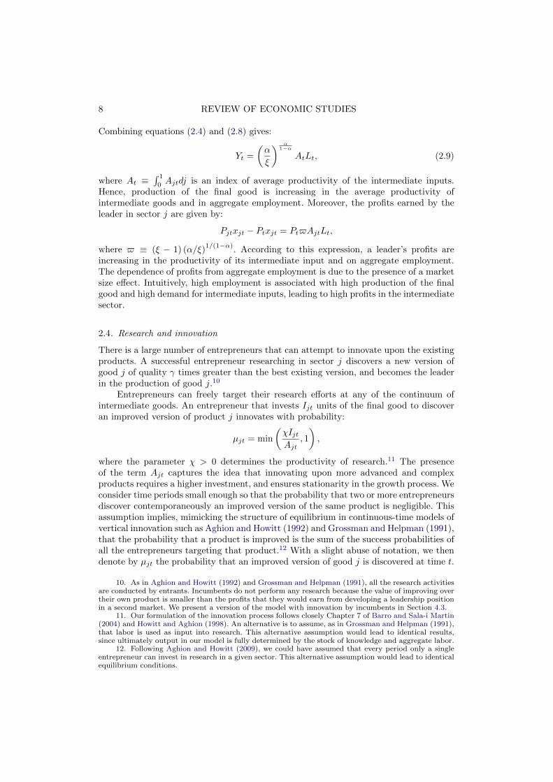
Lu 1
gf
gu
AD
GG
growth
g
employment L
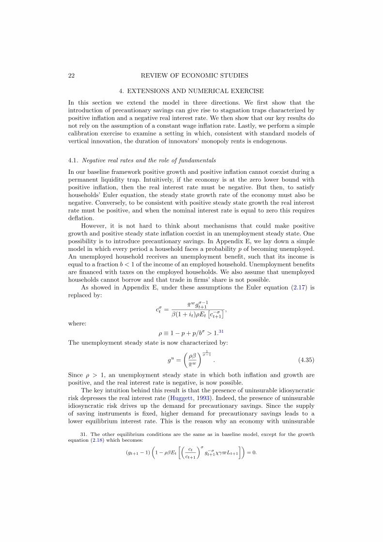
Figure 2Non-stochastic steady states.
bank is constrained by the zero lower bound, and hence monetary policy cannot respondto changes in aggregate demand driven by self-fulfilling expectations.
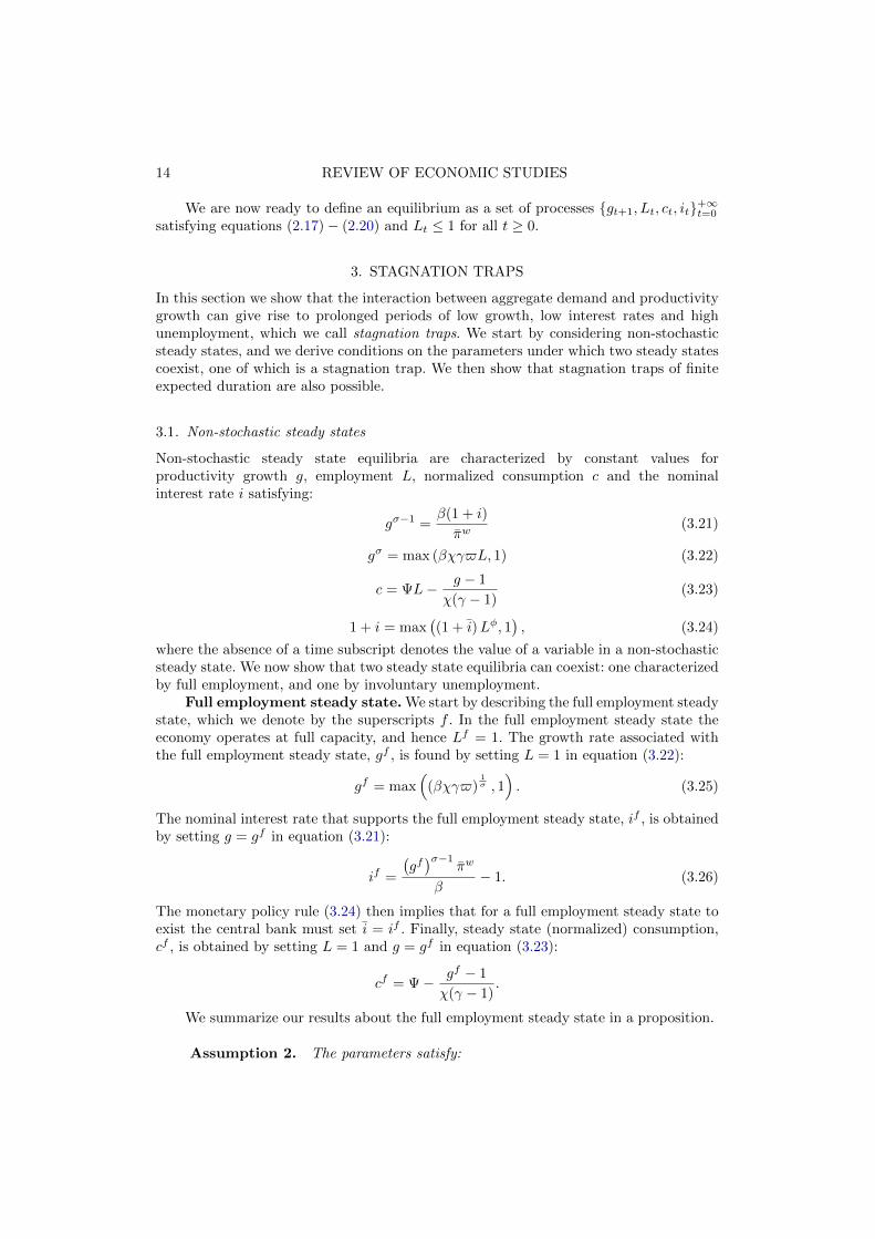
We think of this second steady state as a stagnation trap, that is the combinationof a liquidity and a growth trap. In a liquidity trap the economy operates below capacitybecause the central bank is constrained by the zero lower bound on the nominal interestrate. In a growth trap, lack of demand for firms’ products depresses investment ininnovation and prevents the economy from developing its full growth potential. In astagnation trap these two events are tightly connected. We illustrate this point with thehelp of a diagram.
Figure 2 depicts the two key relationships that characterize the steady states of ourmodel in the L−g space. The first one is the growth equation (3.22), which corresponds tothe GG schedule. For sufficiently high L, the GG schedule is upward sloped. The positiverelationship between L and G can be explained with the fact that, for L high enough,an increase in employment and production is associated with a rise in firms’ profits,while higher profits generate an increase in investment in innovation and productivitygrowth. Instead, for low values of L the GG schedule is horizontal. These are the valuesof employment for which investing in research is not profitable, and hence they areassociated with zero growth.
The second key relationship combines the Euler equation (3.21) and the policy rule(3.24):
gσ−1 =β
πwmax
((1 + i)Lφ, 1
).
Graphically, this relationship is captured by the AD, i.e. aggregate demand, curve. Theupward-sloped portion of the AD curve corresponds to cases in which the zero lowerbound constraint on the nominal interest rate is not binding.26 In this part of the statespace, the central bank responds to a rise in employment by increasing the nominalrate. In turn, to be consistent with households’ Euler equation, a higher interest ratemust be coupled with faster productivity growth.27 Hence, when monetary policy is notconstrained by the zero lower bound the AD curve generates a positive relationshipbetween L and g. Instead, the horizontal portion of the AD curve corresponds to values
26. Precisely, the zero lower bound constraint does not bind when L ≥ (1 + i)−1/φ.27. Recall that we are focusing on the case σ > 1.
18 REVIEW OF ECONOMIC STUDIES
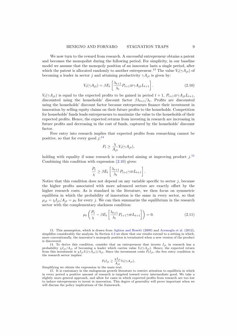
1
gf
AD
GG
growth
g
employment L 1
gf
AD
GG
growth
g
employment L
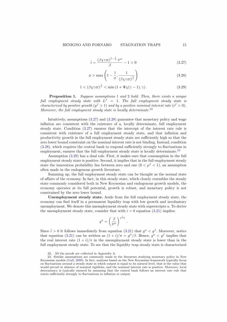
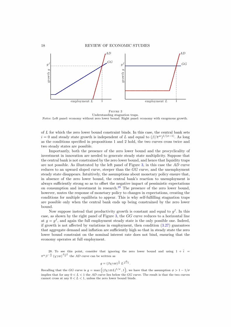
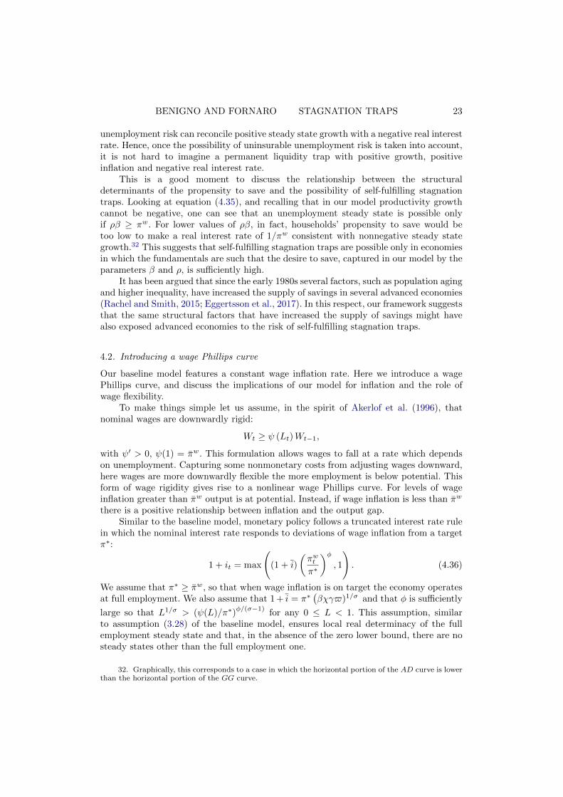
Figure 3Understanding stagnation traps.
Notes: Left panel: economy without zero lower bound. Right panel: economy with exogenous growth.
of L for which the zero lower bound constraint binds. In this case, the central bank setsi = 0 and steady state growth is independent of L and equal to (β/πw)1/(σ−1). As longas the conditions specified in propositions 1 and 2 hold, the two curves cross twice andtwo steady states are possible.
Importantly, both the presence of the zero lower bound and the procyclicality ofinvestment in innovation are needed to generate steady state multiplicity. Suppose thatthe central bank is not constrained by the zero lower bound, and hence that liquidity trapsare not possible. As illustrated by the left panel of Figure 3, in this case the AD curvereduces to an upward sloped curve, steeper than the GG curve, and the unemploymentsteady state disappears. Intuitively, the assumptions about monetary policy ensure that,in absence of the zero lower bound, the central bank’s reaction to unemployment isalways sufficiently strong so as to offset the negative impact of pessimistic expectationson consumption and investment in research.28 The presence of the zero lower bound,however, mutes the response of monetary policy to changes in expectations, creating theconditions for multiple equilibria to appear. This is why self-fulfilling stagnation trapsare possible only when the central bank ends up being constrained by the zero lowerbound.
Now suppose instead that productivity growth is constant and equal to gf . In thiscase, as shown by the right panel of Figure 3, the GG curve reduces to a horizontal lineat g = gf , and again the full employment steady state is the only possible one. Indeed,if growth is not affected by variations in employment, then condition (3.27) guaranteesthat aggregate demand and inflation are sufficiently high so that in steady state the zerolower bound constraint on the nominal interest rate does not bind, ensuring that theeconomy operates at full employment.
28. To see this point, consider that ignoring the zero lower bound and using 1 + i =
πwβ−1σ (χγ$)
σ−1σ the AD curve can be written as
g = (βχγ$)1σ L
φσ−1 .
Recalling that the GG curve is g = max(
(βχγ$L)1/σ , 1)
, we have that the assumption φ > 1 − 1/σ
implies that for any 0 < L < 1 the AD curve lies below the GG curve. The result is that the two curvescannot cross at any 0 < L < 1, unless the zero lower bound binds.
BENIGNO AND FORNARO STAGNATION TRAPS 19
5 10 15 201
1.5
2
2.5
Growth rate
percent
t ime
productivityoutput
5 10 15 20
0
0.5
1
1.5
2
2.5
3Unemployment
percent
t ime5 10 15 20
0
0.5
1
1.5
Nominal rate
percent
time
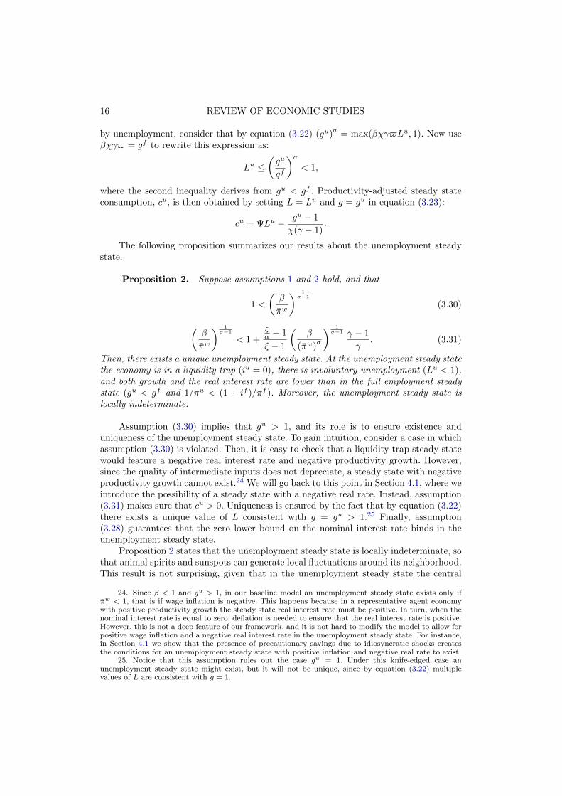
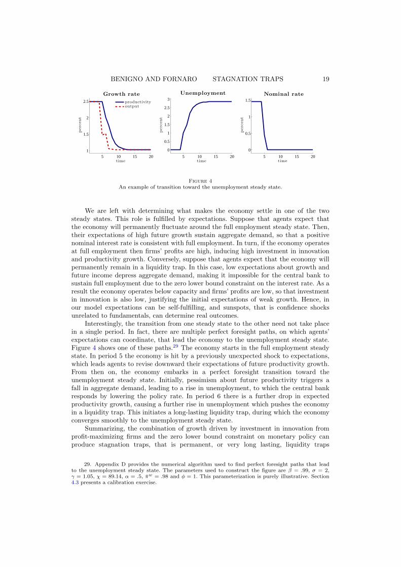
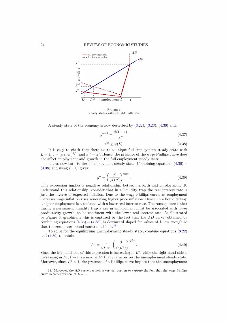
Figure 4An example of transition toward the unemployment steady state.
We are left with determining what makes the economy settle in one of the twosteady states. This role is fulfilled by expectations. Suppose that agents expect thatthe economy will permanently fluctuate around the full employment steady state. Then,their expectations of high future growth sustain aggregate demand, so that a positivenominal interest rate is consistent with full employment. In turn, if the economy operatesat full employment then firms’ profits are high, inducing high investment in innovationand productivity growth. Conversely, suppose that agents expect that the economy willpermanently remain in a liquidity trap. In this case, low expectations about growth andfuture income depress aggregate demand, making it impossible for the central bank tosustain full employment due to the zero lower bound constraint on the interest rate. As aresult the economy operates below capacity and firms’ profits are low, so that investmentin innovation is also low, justifying the initial expectations of weak growth. Hence, inour model expectations can be self-fulfilling, and sunspots, that is confidence shocksunrelated to fundamentals, can determine real outcomes.
Interestingly, the transition from one steady state to the other need not take placein a single period. In fact, there are multiple perfect foresight paths, on which agents’expectations can coordinate, that lead the economy to the unemployment steady state.Figure 4 shows one of these paths.29 The economy starts in the full employment steadystate. In period 5 the economy is hit by a previously unexpected shock to expectations,which leads agents to revise downward their expectations of future productivity growth.From then on, the economy embarks in a perfect foresight transition toward theunemployment steady state. Initially, pessimism about future productivity triggers afall in aggregate demand, leading to a rise in unemployment, to which the central bankresponds by lowering the policy rate. In period 6 there is a further drop in expectedproductivity growth, causing a further rise in unemployment which pushes the economyin a liquidity trap. This initiates a long-lasting liquidity trap, during which the economyconverges smoothly to the unemployment steady state.
Summarizing, the combination of growth driven by investment in innovation fromprofit-maximizing firms and the zero lower bound constraint on monetary policy canproduce stagnation traps, that is permanent, or very long lasting, liquidity traps
29. Appendix D provides the numerical algorithm used to find perfect foresight paths that leadto the unemployment steady state. The parameters used to construct the figure are β = .99, σ = 2,γ = 1.05, χ = 89.14, α = .5, πw = .98 and φ = 1. This parameterization is purely illustrative. Section4.3 presents a calibration exercise.
20 REVIEW OF ECONOMIC STUDIES
characterized by unemployment and low growth. All it takes is a sunspot that coordinatesagents’ expectations on a path that leads to the unemployment steady state.
Before moving on, it is useful to compare our notion of stagnation traps with thepermanent liquidity traps that can arise in the New Keynesian model. In the standardNew Keynesian model productivity growth is exogenous, and there is a unique realinterest rate consistent with a steady state. As shown by Benhabib et al. (2001),permanent liquidity traps can occur in these frameworks if agents coordinate theirexpectations on an inflation rate equal to the inverse of the steady state real interestrate. Because of this, the New Keynesian model typically feature two steady states, oneof which is a permanent liquidity trap. These two steady states are characterized bythe same real interest rate, but by different inflation and nominal interest rates, withthe liquidity trap steady state being associated with inflation below the central bank’starget.
In contrast, in our framework endogenous growth is key in opening the door to steadystate multiplicity and permanent liquidity traps. Crucially, in our model the two steadystates feature different growth and real interest rates, with the liquidity trap steadystate being associated with low growth and low real interest rate. Instead, inflationexpectations do not play a major role. In fact, once a wage Phillips curve is introducedin the model, it might very well be the case that inflation in the unemployment steadystate is the same, or even higher, than in the full employment one. We will go back tothis point in Section 4.2.
3.2. Temporary stagnation traps
Though our model can allow for economies which are permanently in a liquidity trap, itis not difficult to construct equilibria in which the expected duration of a trap is finite.To construct an equilibrium featuring a temporary liquidity trap we have to put somestructure on the sunspot process. Let us start by denoting a sunspot by ξt. In a sunspotequilibrium agents form their expectations about the future after observing ξt, so thatthe sunspot acts as a coordination device for agents’ expectations. Following Mertensand Ravn (2014), let us consider a two-state discrete Markov process, ξt ∈ (ξo, ξp), withtransition probabilities Pr (ξt+1 = ξo|ξt = ξo) = 1 and Pr (ξt+1 = ξp|ξt = ξp) = q < 1.The first state is an absorbing optimistic equilibrium, in which agents expect to remainforever around the full employment steady state. Hence, once ξt = ξo the economy settleson the full employment steady state, characterized by L = 1 and g = gf . The secondstate ξp is a pessimistic equilibrium with finite expected duration 1/(1− q). In this statethe economy is in a liquidity trap with unemployment. We consider an economy thatstarts in the pessimistic equilibrium.
Under these assumptions, as long as the pessimistic sunspot shock persists theequilibrium is described by equations (2.17), (2.18) and (2.19), which, using the factthat in the pessimistic state i = 0, can be written as:
(gp)σ−1
=β
πw
(q + (1− q)
(cp
cf
)σ)(3.32)
(gp − 1)
((gp)
σ − βχγ$(qLp + (1− q)
(cp
cf
)σ))= 0. (3.33)
cp = ΨLp − gp − 1
χ(γ − 1), (3.34)
BENIGNO AND FORNARO STAGNATION TRAPS 21
10 20 30
1
1.5
2
Productivity growth
percent
t ime10 20 30
0.5
1
1.5
2
2.5
3
3.5
Unemployment
percent
t ime10 20 30
0
0.5
1
1.5Nominal rate
percent
time
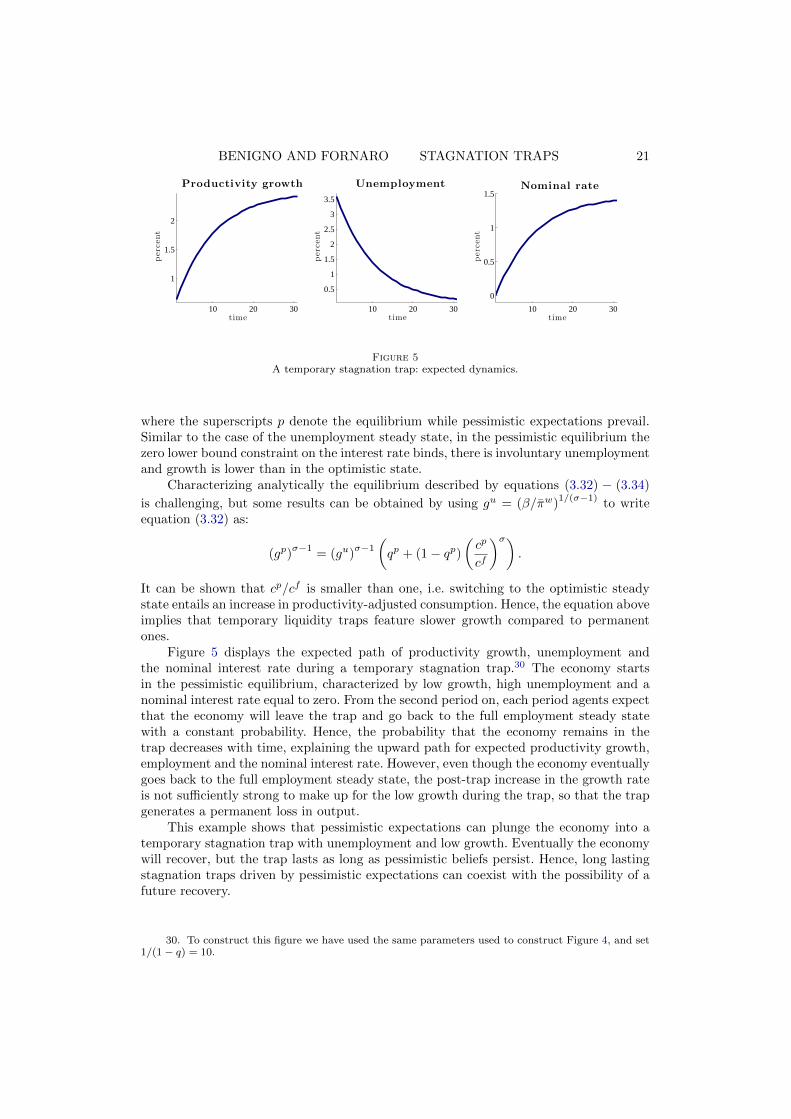
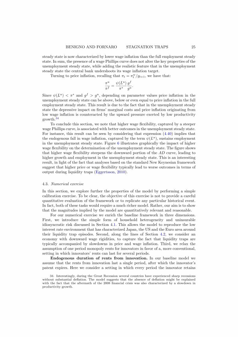
Figure 5A temporary stagnation trap: expected dynamics.
where the superscripts p denote the equilibrium while pessimistic expectations prevail.Similar to the case of the unemployment steady state, in the pessimistic equilibrium thezero lower bound constraint on the interest rate binds, there is involuntary unemploymentand growth is lower than in the optimistic state.
Characterizing analytically the equilibrium described by equations (3.32) − (3.34)
is challenging, but some results can be obtained by using gu = (β/πw)1/(σ−1)
to writeequation (3.32) as:
(gp)σ−1
= (gu)σ−1
(qp + (1− qp)
(cp
cf
)σ).
It can be shown that cp/cf is smaller than one, i.e. switching to the optimistic steadystate entails an increase in productivity-adjusted consumption. Hence, the equation aboveimplies that temporary liquidity traps feature slower growth compared to permanentones.
Figure 5 displays the expected path of productivity growth, unemployment andthe nominal interest rate during a temporary stagnation trap.30 The economy startsin the pessimistic equilibrium, characterized by low growth, high unemployment and anominal interest rate equal to zero. From the second period on, each period agents expectthat the economy will leave the trap and go back to the full employment steady statewith a constant probability. Hence, the probability that the economy remains in thetrap decreases with time, explaining the upward path for expected productivity growth,employment and the nominal interest rate. However, even though the economy eventuallygoes back to the full employment steady state, the post-trap increase in the growth rateis not sufficiently strong to make up for the low growth during the trap, so that the trapgenerates a permanent loss in output.
This example shows that pessimistic expectations can plunge the economy into atemporary stagnation trap with unemployment and low growth. Eventually the economywill recover, but the trap lasts as long as pessimistic beliefs persist. Hence, long lastingstagnation traps driven by pessimistic expectations can coexist with the possibility of afuture recovery.
30. To construct this figure we have used the same parameters used to construct Figure 4, and set1/(1− q) = 10.
22 REVIEW OF ECONOMIC STUDIES
4. EXTENSIONS AND NUMERICAL EXERCISE
In this section we extend the model in three directions. We first show that theintroduction of precautionary savings can give rise to stagnation traps characterized bypositive inflation and a negative real interest rate. We then show that our key results donot rely on the assumption of a constant wage inflation rate. Lastly, we perform a simplecalibration exercise to examine a setting in which, consistent with standard models ofvertical innovation, the duration of innovators’ monopoly rents is endogenous.
4.1. Negative real rates and the role of fundamentals
In our baseline framework positive growth and positive inflation cannot coexist during apermanent liquidity trap. Intuitively, if the economy is at the zero lower bound withpositive inflation, then the real interest rate must be negative. But then, to satisfyhouseholds’ Euler equation, the steady state growth rate of the economy must also benegative. Conversely, to be consistent with positive steady state growth the real interestrate must be positive, and when the nominal interest rate is equal to zero this requiresdeflation.
However, it is not hard to think about mechanisms that could make positivegrowth and positive steady state inflation coexist in an unemployment steady state. Onepossibility is to introduce precautionary savings. In Appendix E, we lay down a simplemodel in which every period a household faces a probability p of becoming unemployed.An unemployed household receives an unemployment benefit, such that its income isequal to a fraction b < 1 of the income of an employed household. Unemployment benefitsare financed with taxes on the employed households. We also assume that unemployedhouseholds cannot borrow and that trade in firms’ share is not possible.
As showed in Appendix E, under these assumptions the Euler equation (2.17) isreplaced by:
cσt =πwgσ−1t+1
β(1 + it)ρEt[c−σt+1
] ,where:
ρ ≡ 1− p+ p/bσ > 1.31
The unemployment steady state is now characterized by:
gu =
(ρβ
πw
) 1σ−1
. (4.35)
Since ρ > 1, an unemployment steady state in which both inflation and growth arepositive, and the real interest rate is negative, is now possible.
The key intuition behind this result is that the presence of uninsurable idiosyncraticrisk depresses the real interest rate (Huggett, 1993). Indeed, the presence of uninsurableidiosyncratic risk drives up the demand for precautionary savings. Since the supplyof saving instruments is fixed, higher demand for precautionary savings leads to alower equilibrium interest rate. This is the reason why an economy with uninsurable
31. The other equilibrium conditions are the same as in baseline model, except for the growthequation (2.18) which becomes:
(gt+1 − 1)
(1− ρβEt
[(ct
ct+1
)σg−σt+1χγ$Lt+1
])= 0.
BENIGNO AND FORNARO STAGNATION TRAPS 23
unemployment risk can reconcile positive steady state growth with a negative real interestrate. Hence, once the possibility of uninsurable unemployment risk is taken into account,it is not hard to imagine a permanent liquidity trap with positive growth, positiveinflation and negative real interest rate.
This is a good moment to discuss the relationship between the structuraldeterminants of the propensity to save and the possibility of self-fulfilling stagnationtraps. Looking at equation (4.35), and recalling that in our model productivity growthcannot be negative, one can see that an unemployment steady state is possible onlyif ρβ ≥ πw. For lower values of ρβ, in fact, households’ propensity to save would betoo low to make a real interest rate of 1/πw consistent with nonnegative steady stategrowth.32 This suggests that self-fulfilling stagnation traps are possible only in economiesin which the fundamentals are such that the desire to save, captured in our model by theparameters β and ρ, is sufficiently high.
It has been argued that since the early 1980s several factors, such as population agingand higher inequality, have increased the supply of savings in several advanced economies(Rachel and Smith, 2015; Eggertsson et al., 2017). In this respect, our framework suggeststhat the same structural factors that have increased the supply of savings might havealso exposed advanced economies to the risk of self-fulfilling stagnation traps.
4.2. Introducing a wage Phillips curve
Our baseline model features a constant wage inflation rate. Here we introduce a wagePhillips curve, and discuss the implications of our model for inflation and the role ofwage flexibility.
To make things simple let us assume, in the spirit of Akerlof et al. (1996), thatnominal wages are downwardly rigid:
Wt ≥ ψ (Lt)Wt−1,
with ψ′ > 0, ψ(1) = πw. This formulation allows wages to fall at a rate which dependson unemployment. Capturing some nonmonetary costs from adjusting wages downward,here wages are more downwardly flexible the more employment is below potential. Thisform of wage rigidity gives rise to a nonlinear wage Phillips curve. For levels of wageinflation greater than πw output is at potential. Instead, if wage inflation is less than πw
there is a positive relationship between inflation and the output gap.Similar to the baseline model, monetary policy follows a truncated interest rate rule
in which the nominal interest rate responds to deviations of wage inflation from a targetπ∗:
1 + it = max
((1 + i)
(πwtπ∗
)φ, 1
). (4.36)
We assume that π∗ ≥ πw, so that when wage inflation is on target the economy operatesat full employment. We also assume that 1 + i = π∗
(βχγ$)1/σ and that φ is sufficiently
large so that L1/σ > (ψ(L)/π∗)φ/(σ−1) for any 0 ≤ L < 1. This assumption, similarto assumption (3.28) of the baseline model, ensures local real determinacy of the fullemployment steady state and that, in the absence of the zero lower bound, there are nosteady states other than the full employment one.
32. Graphically, this corresponds to a case in which the horizontal portion of the AD curve is lowerthan the horizontal portion of the GG curve.
24 REVIEW OF ECONOMIC STUDIES
Lu Lu′ 1
gf
gu
gu′
AD
GG
growth
g
employment L
AD low wage flex.AD high wage flex.
Figure 6Steady states with variable inflation.
A steady state of the economy is now described by (3.22), (3.23), (4.36) and:
gσ−1 =β(1 + i)
πw(4.37)
πw ≥ ψ(L). (4.38)
It is easy to check that there exists a unique full employment steady state withL = 1, g = (βχγ$)1/σ and πw = π∗. Hence, the presence of the wage Phillips curve doesnot affect employment and growth in the full employment steady state.
Let us now turn to the unemployment steady state. Combining equations (4.36) −(4.38) and using i = 0, gives:
gu =
(β
ψ(Lu)
) 1σ−1
. (4.39)
This expression implies a negative relationship between growth and employment. Tounderstand this relationship, consider that in a liquidity trap the real interest rate isjust the inverse of expected inflation. Due to the wage Phillips curve, as employmentincreases wage inflation rises generating higher price inflation. Hence, in a liquidity trapa higher employment is associated with a lower real interest rate. The consequence is thatduring a permanent liquidity trap a rise in employment must be associated with lowerproductivity growth, to be consistent with the lower real interest rate. As illustratedby Figure 6, graphically this is captured by the fact that the AD curve, obtained bycombining equations (4.36) − (4.38), is downward sloped for values of L low enough sothat the zero lower bound constraint binds.33
To solve for the equilibrium unemployment steady state, combine equations (3.22)and (4.39) to obtain:
Lu =1
βχγ$
(β
ψ(Lu)
) σσ−1
. (4.40)
Since the left-hand side of this expression is increasing in Lu, while the right hand-side isdecreasing in Lu, there is a unique Lu that characterizes the unemployment steady state.Moreover, since Lu < 1, the presence of a Phillips curve implies that the unemployment
33. Moreover, the AD curve has now a vertical portion to capture the fact that the wage Phillipscurve becomes vertical at L = 1.
BENIGNO AND FORNARO STAGNATION TRAPS 25
steady state is now characterized by lower wage inflation than the full employment steadystate. In sum, the presence of a wage Phillips curve does not alter the key properties of theunemployment steady state, while adding the realistic feature that in the unemploymentsteady state the central bank undershoots its wage inflation target.
Turning to price inflation, recalling that πt = πwt /gt+1, we have that:
πu
πf=ψ(Lu)
π∗gf
gu.
Since ψ(Lu) < π∗ and gf > gu, depending on parameter values price inflation in theunemployment steady state can be above, below or even equal to price inflation in the fullemployment steady state. This result is due to the fact that in the unemployment steadystate the depressive impact on firms’ marginal costs and price inflation originating fromlow wage inflation is counteracted by the upward pressure exerted by low productivitygrowth.34
To conclude this section, we note that higher wage flexibility, captured by a steeperwage Phillips curve, is associated with better outcomes in the unemployment steady state.For instance, this result can be seen by considering that expression (4.40) implies thatthe endogenous fall in wage inflation, captured by the term ψ(Lu), sustains employmentin the unemployment steady state. Figure 6 illustrates graphically the impact of higherwage flexibility on the determination of the unemployment steady state. The figure showsthat higher wage flexibility steepens the downward portion of the AD curve, leading tohigher growth and employment in the unemployment steady state. This is an interestingresult, in light of the fact that analyses based on the standard New Keynesian frameworksuggest that higher price or wage flexibility typically lead to worse outcomes in terms ofoutput during liquidity traps (Eggertsson, 2010).
4.3. Numerical exercise
In this section, we explore further the properties of the model by performing a simplecalibration exercise. To be clear, the objective of this exercise is not to provide a carefulquantitative evaluation of the framework or to replicate any particular historical event.In fact, both of these tasks would require a much richer model. Rather, our aim is to showthat the magnitudes implied by the model are quantitatively relevant and reasonable.
For our numerical exercise we enrich the baseline framework in three dimensions.First, we introduce the simple form of household heterogeneity and uninsurableidiosyncratic risk discussed in Section 4.1. This allows the model to reproduce the lowinterest rate environment that has characterized Japan, the US and the Euro area aroundtheir liquidity trap episodes. Second, along the lines of Section 4.2, we consider aneconomy with downward wage rigidities, to capture the fact that liquidity traps aretypically accompanied by slowdowns in price and wage inflation. Third, we relax theassumption of one period monopoly rents for innovators in favor of a, more conventional,setting in which innovators’ rents can last for several periods.
Endogenous duration of rents from innovation. In our baseline model weassume that the rents from innovation last a single period, after which the innovator’spatent expires. Here we consider a setting in which every period the innovator retains
34. Interestingly, during the Great Recession several countries have experienced sharp recessionswithout substantial deflation. The model suggests that the absence of deflation might be explainedwith the fact that the aftermath of the 2008 financial crisis was also characterized by a slowdown inproductivity growth.
26 REVIEW OF ECONOMIC STUDIES
its patent with probability 1 − η.35 As in the baseline mode, after the patent is lostthe monopoly position is allocated randomly to another entrepreneur. Under theseassumptions, the value of becoming a leader in sector j is:
Vt(γAjt) = βρEt
[λt+1
λt(Pt+1$γAjtLt+1 + (1− µjt+1 − η)Vt+1(γAjt))
], (4.41)
where µj,t+1 + η ≤ 1. The first term inside the parenthesis on the right-hand side, alsopresent in the baseline model, captures the expected profits to be gained in period t+ 1.In addition, the value of a successful innovation includes the value of being a leader inperiod t+ 1, Vt+1(γAjt), times the probability that the entrepreneur remains the leaderin period t+ 1, 1− µjt+1 − η. Notice that the probability of maintaining the leadershipis decreasing in µjt+1, due to the fact that the discovery of a better version of productj terminates the monopoly rents for the incumbent. Future payoffs are discounted usingthe households’ discount factor βρλt+1/λt, which is now adjusted for the presence ofidiosyncratic risk.
To streamline the exposition, in this section we restrict attention to equilibria inwhich in every period a positive amount of research is targeted toward every intermediategood.36 In this case, free entry into research implies that expected profits from researchingare zero for every product. This zero profit condition implies that:37
Pt =χ
AjtVt(γAjt),
for every good j. Moreover, we focus on symmetric equilibria in which the probability ofinnovation is the same in every sector, so that µjt = χIjt/Ajt = µt for every j. In thiscase, Vt(γAjt) = VtγAjt for every j, while free entry into the research sector in periodt+1 implies Vt+1 = Pt+1/(γχ). Combining these conditions with expression (4.41) gives:
Ptχ
= βρEt
[λt+1
λt
(Pt+1$γLt+1 + (1− µt+1 − η)
Pt+1
χ
)].
This expression summarizes the equilibrium in the research sector. Combining thisexpression with equation (2.2) and using µt = (gt+1 − 1)/(χ(γ − 1)) gives:
gσt+1 = βρEt
[(ctct+1
)σ (χγ$Lt+1 + 1− gt+2 − 1
γ − 1− η)]
, (4.42)
which replaces equation (2.18) of the baseline model.Parameters. We choose the length of a period to correspond to a year. We set the
inverse of the elasticity of intertemporal substitution to σ = 2 and the discount factorto β = 0.994 = 0.96, in the range of the values commonly considered by the business-cycle literature. We target a real interest rate in the full employment steady state of 1.5
35. Standard models of vertical innovation typically assume that η = 0. Instead, we followAcemoglu and Akcigit (2012) and consider the case η > 0. This assumption encapsulates all the factorsthat might lead to the termination of the rents from innovation besides innovation by entrants. Theseinclude patent expiration and imitation by competitors.
36. We verify that this condition holds in all the simulations presented below.37. To derive this condition, consider that an entrepreneur that invests Ijt in research has a
probability χIjt/Ajt of becoming a leader which carries value Vt(γAjt). Hence, the expected returnfrom this investment is χIjtVt(γAjt)/Ajt. Since the investment costs PtIjt, the zero expected profitscondition in the research sector implies:
PtIjt =χIjt
AjtVt(γAjt).
Simplifying we obtain the expression in the main text.
BENIGNO AND FORNARO STAGNATION TRAPS 27
percent, in line with the low interest rates characterizing the US and the Euro area inthe run-up to the 2008 financial crisis, and a growth rate in the full employment steadystate of 2 percent. Using 1 + rf = (gf )σ/(ρβ), these targets imply ρ = 1.067.38 Thecentral bank’s wage inflation target is set to π∗ = 1.04, so that price inflation in the fullemployment steady state is 2 percent.
Turning to the parameters determining the growth process, we set the labor sharein gross output to 1 − α = 0.83, to match a ratio of spending in R&D-to-GDP in thefull employment steady state of 2 percent, close to the long-run average of the businessspending in R&D-to-GDP ratio in the US.39 The step size of innovations is set to γ = 1.55so that the probability that an innovation occurs in a given sector is 3.6 percent per year,as in Howitt (2000). We choose the value of χ, the parameter determining the productivityof research, to match our 2 percent growth target in the full employment steady state. Toset the parameter η we follow the same strategy adopted by Kung and Schmid (2015), andassume that the probability that the rents from innovation expire in the full employmentsteady state, given by µf + η, is equal to 15%, the rate of depreciation of the R&D stockestimated by the Bureau of Labor Statistics.40
We perform the following experiment. We target a value for the output gap in theunemployment steady state, and derive the implications for growth, the real interest rate,and price and wage inflation.41 Estimates of the output gap for the Japanese slump liebetween 5 and 10 percent (Hausman and Wieland, 2014). This is roughly in line withthe range of estimates for the output gap during the post-crisis liquidity traps in the US(Del Negro et al., 2015; CBO, 2017) and in the Euro area (Jarocinski and Lenza, 2016).As our baseline, we thus assume that in the unemployment steady state output is 7.5%below potential. Since in our model deviations of output from potential are purely dueto unemployment, this implies setting 1 − Lu = 0.075.42 We later show how the resultschange as the distance of output from potential varies between 5 and 10 percent.
Notice that across our simulations we keep ρ, the parameter capturing the impactof idiosyncratic risk on savings, constant. This means that we are abstracting from theimpact that changes in employment L might have on idiosyncratic unemployment risk.43
38. To gain intuition about the plausibility of this value of ρ, consider a case in which p = 0.05, sothat every household faces a constant 5 percent probability of becoming unemployed. Then ρ = 1.067implies a value for unemployment benefits of b = 0.65, in the range of the replacement rates typicallyassumed by the search and matching literature (Hall and Milgrom, 2008).
39. More precisely, in the US during the period between 1953 and 2014 the average ratio of businessspending in R&D over GDP has been 1.7 percent. Here we follow a large part of the endogenous growthliterature that uses spending in R&D as the data counterpart of the model’s investment in innovation.It is also possible, and in our judgement plausible, to take a broader interpretation of investment ininnovation that includes other types of investment, often difficult to measure, that contribute to firms’productivity growth. One example is investment in implementation of existing technologies.
40. To be clear, in our model the stock of knowledge does not depreciate, since when a firm exits dueto patent expiration it is replaced by another equally-productive firm. Alternatively, one could assumethat once a firm exits, for reasons unrelated to creative destruction, its knowledge is lost. This wouldintroduce a positive rate of depreciation in the aggregate stock of knowledge. We have experimentedwith this alternative, and found that the results are not significantly affected.
41. Thus, throughout our simulations we adjust the shape of the wage Phillips curve so that theunemployment steady state features the targeted output gap. This is the same approach adopted byEggertsson et al. (2017).
42. In richer models other factors, such as variable markups or capital utilization, can drive awedge between potential and actual output. Introducing these elements would reduce the amount ofunemployment needed to generate a given amount of output gap.
43. In practice, we are assuming that the rise in unemployment during a stagnation trap manifestsitself through a reduction in hours worked per person employed, rather than in a fall in the number ofpersons employed. This assumption is not made on the ground of realism, but rather to focus on therelationship between growth and interest rates which is at the heart of our framework.
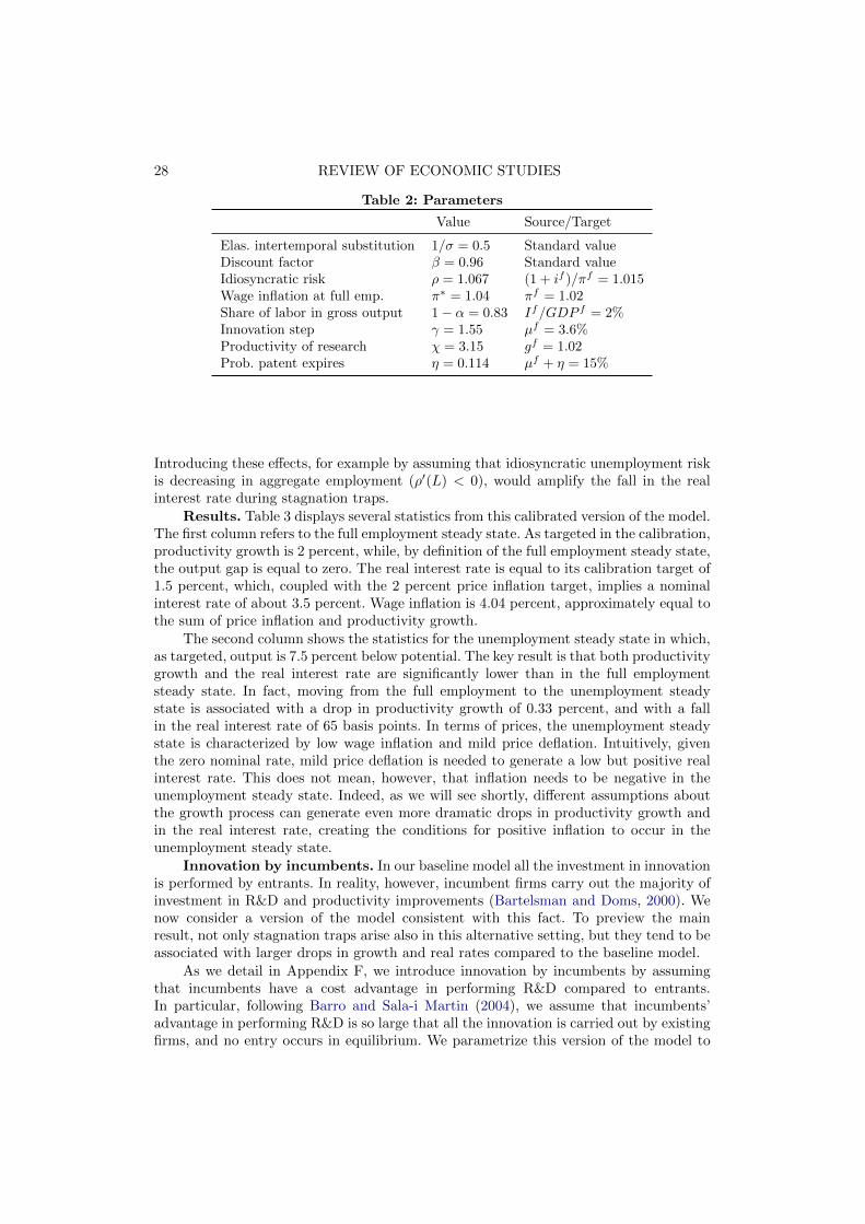
28 REVIEW OF ECONOMIC STUDIES
Table 2: Parameters
Value Source/Target
Elas. intertemporal substitution 1/σ = 0.5 Standard valueDiscount factor β = 0.96 Standard valueIdiosyncratic risk ρ = 1.067 (1 + if )/πf = 1.015Wage inflation at full emp. π∗ = 1.04 πf = 1.02Share of labor in gross output 1− α = 0.83 If/GDP f = 2%Innovation step γ = 1.55 µf = 3.6%Productivity of research χ = 3.15 gf = 1.02Prob. patent expires η = 0.114 µf + η = 15%
Introducing these effects, for example by assuming that idiosyncratic unemployment riskis decreasing in aggregate employment (ρ′(L) < 0), would amplify the fall in the realinterest rate during stagnation traps.
Results. Table 3 displays several statistics from this calibrated version of the model.The first column refers to the full employment steady state. As targeted in the calibration,productivity growth is 2 percent, while, by definition of the full employment steady state,the output gap is equal to zero. The real interest rate is equal to its calibration target of1.5 percent, which, coupled with the 2 percent price inflation target, implies a nominalinterest rate of about 3.5 percent. Wage inflation is 4.04 percent, approximately equal tothe sum of price inflation and productivity growth.
The second column shows the statistics for the unemployment steady state in which,as targeted, output is 7.5 percent below potential. The key result is that both productivitygrowth and the real interest rate are significantly lower than in the full employmentsteady state. In fact, moving from the full employment to the unemployment steadystate is associated with a drop in productivity growth of 0.33 percent, and with a fallin the real interest rate of 65 basis points. In terms of prices, the unemployment steadystate is characterized by low wage inflation and mild price deflation. Intuitively, giventhe zero nominal rate, mild price deflation is needed to generate a low but positive realinterest rate. This does not mean, however, that inflation needs to be negative in theunemployment steady state. Indeed, as we will see shortly, different assumptions aboutthe growth process can generate even more dramatic drops in productivity growth andin the real interest rate, creating the conditions for positive inflation to occur in theunemployment steady state.
Innovation by incumbents. In our baseline model all the investment in innovationis performed by entrants. In reality, however, incumbent firms carry out the majority ofinvestment in R&D and productivity improvements (Bartelsman and Doms, 2000). Wenow consider a version of the model consistent with this fact. To preview the mainresult, not only stagnation traps arise also in this alternative setting, but they tend to beassociated with larger drops in growth and real rates compared to the baseline model.
As we detail in Appendix F, we introduce innovation by incumbents by assumingthat incumbents have a cost advantage in performing R&D compared to entrants.In particular, following Barro and Sala-i Martin (2004), we assume that incumbents’advantage in performing R&D is so large that all the innovation is carried out by existingfirms, and no entry occurs in equilibrium. We parametrize this version of the model to
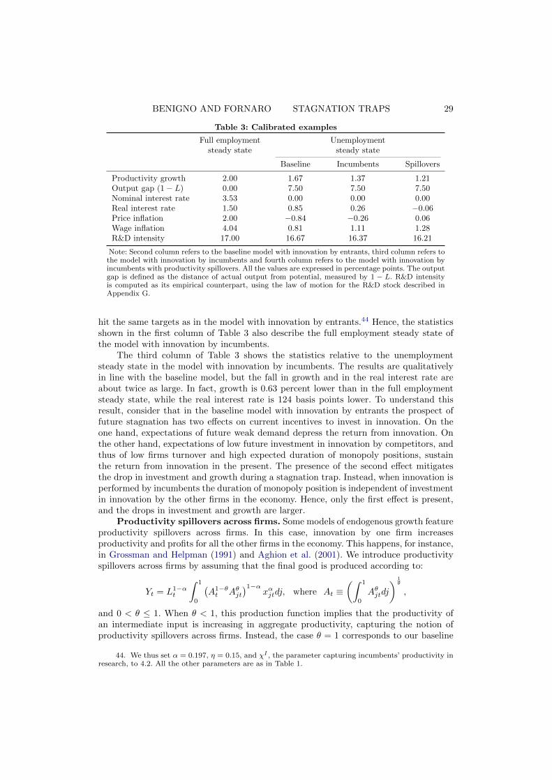
BENIGNO AND FORNARO STAGNATION TRAPS 29
Table 3: Calibrated examples
Full employment Unemploymentsteady state steady state
Baseline Incumbents Spillovers
Productivity growth 2.00 1.67 1.37 1.21Output gap (1− L) 0.00 7.50 7.50 7.50Nominal interest rate 3.53 0.00 0.00 0.00Real interest rate 1.50 0.85 0.26 −0.06Price inflation 2.00 −0.84 −0.26 0.06Wage inflation 4.04 0.81 1.11 1.28R&D intensity 17.00 16.67 16.37 16.21
Note: Second column refers to the baseline model with innovation by entrants, third column refers tothe model with innovation by incumbents and fourth column refers to the model with innovation byincumbents with productivity spillovers. All the values are expressed in percentage points. The outputgap is defined as the distance of actual output from potential, measured by 1 − L. R&D intensityis computed as its empirical counterpart, using the law of motion for the R&D stock described inAppendix G.
hit the same targets as in the model with innovation by entrants.44 Hence, the statisticsshown in the first column of Table 3 also describe the full employment steady state ofthe model with innovation by incumbents.
The third column of Table 3 shows the statistics relative to the unemploymentsteady state in the model with innovation by incumbents. The results are qualitativelyin line with the baseline model, but the fall in growth and in the real interest rate areabout twice as large. In fact, growth is 0.63 percent lower than in the full employmentsteady state, while the real interest rate is 124 basis points lower. To understand thisresult, consider that in the baseline model with innovation by entrants the prospect offuture stagnation has two effects on current incentives to invest in innovation. On theone hand, expectations of future weak demand depress the return from innovation. Onthe other hand, expectations of low future investment in innovation by competitors, andthus of low firms turnover and high expected duration of monopoly positions, sustainthe return from innovation in the present. The presence of the second effect mitigatesthe drop in investment and growth during a stagnation trap. Instead, when innovation isperformed by incumbents the duration of monopoly position is independent of investmentin innovation by the other firms in the economy. Hence, only the first effect is present,and the drops in investment and growth are larger.
Productivity spillovers across firms. Some models of endogenous growth featureproductivity spillovers across firms. In this case, innovation by one firm increasesproductivity and profits for all the other firms in the economy. This happens, for instance,in Grossman and Helpman (1991) and Aghion et al. (2001). We introduce productivityspillovers across firms by assuming that the final good is produced according to:
Yt = L1−αt
∫ 1
0
(A1−θt Aθjt
)1−αxαjtdj, where At ≡
(∫ 1
0
Aθjtdj
) 1θ
,
and 0 < θ ≤ 1. When θ < 1, this production function implies that the productivity ofan intermediate input is increasing in aggregate productivity, capturing the notion ofproductivity spillovers across firms. Instead, the case θ = 1 corresponds to our baseline
44. We thus set α = 0.197, η = 0.15, and χI , the parameter capturing incumbents’ productivity inresearch, to 4.2. All the other parameters are as in Table 1.
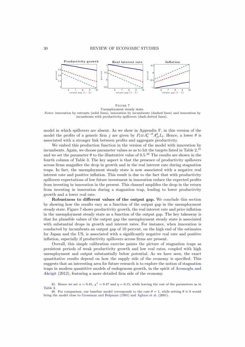
30 REVIEW OF ECONOMIC STUDIES
6 7 8 9 101
1.2
1.4
1.6
Productivity growth
perc
ent
output gap (1 − L)6 7 8 9 10
−0.5
0
0.5
1Real interest rate
perc
ent
output gap (1 − L)6 7 8 9 10
−1
−0.5
0
0.5
Inflation
perc
ent
output gap (1 − L)
Figure 7Unemployment steady state.
Notes: innovation by entrants (solid lines), innovation by incumbents (dashed lines) and innovation byincumbents with productivity spillovers (dash-dotted lines).
model in which spillovers are absent. As we show in Appendix F, in this version of themodel the profits of a generic firm j are given by Pt$A
1−θt AθjtLt. Hence, a lower θ is
associated with a stronger link between profits and aggregate productivity.We embed this production function in the version of the model with innovation by
incumbents. Again, we choose parameter values so as to hit the targets listed in Table 2,45
and we set the parameter θ to the illustrative value of 0.5.46 The results are shown in thefourth column of Table 3. The key aspect is that the presence of productivity spilloversacross firms magnifies the drop in growth and in the real interest rate during stagnationtraps. In fact, the unemployment steady state is now associated with a negative realinterest rate and positive inflation. This result is due to the fact that with productivityspillovers expectations of low future investment in innovation reduce the expected profitsfrom investing in innovation in the present. This channel amplifies the drop in the returnfrom investing in innovation during a stagnation trap, leading to lower productivitygrowth and a lower real rate.
Robustness to different values of the output gap. We conclude this sectionby showing how the results vary as a function of the output gap in the unemploymentsteady state. Figure 7 shows productivity growth, the real interest rate and price inflationin the unemployment steady state as a function of the output gap. The key takeaway isthat for plausible values of the output gap the unemployment steady state is associatedwith substantial drops in growth and interest rates. For instance, when innovation isconducted by incumbents an output gap of 10 percent, on the high end of the estimatesfor Japan and the US, is associated with a significantly negative real rate and positiveinflation, especially if productivity spillovers across firms are present.
Overall, this simple calibration exercise paints the picture of stagnation traps aspersistent periods of weak productivity growth and low real rates, coupled with highunemployment and output substantially below potential. As we have seen, the exactquantitative results depend on how the supply side of the economy is specified. Thissuggests that an interesting area for future research is to explore the notion of stagnationtraps in modern quantitive models of endogenous growth, in the spirit of Acemoglu andAkcigit (2012), featuring a more detailed firm side of the economy.
45. Hence we set α = 0.45, χI = 9.47 and η = 0.15, while leaving the rest of the parameters as inTable 2.
46. For comparison, our baseline model corresponds to the case θ = 1, while setting θ ≈ 0 wouldbring the model close to Grossman and Helpman (1991) and Aghion et al. (2001).
BENIGNO AND FORNARO STAGNATION TRAPS 31
5. POLICY IMPLICATIONS
Which policy interventions can push the economy out of a stagnation trap? To addressthis question, we first consider monetary policy interventions. We then turn to growthpolicies, aiming at sustaining investment in productivity enhancing activities. Forsimplicity, we discuss the role of these policies in the context of the baseline modeldescribed in Section 2.
5.1. Monetary policy
In Section 3 we have shown that stagnation traps can arise if the central bank followsan interest rate rule, in which the interest rate responds monotonically to employmentor wage inflation. In this section we examine the robustness of this result to alternativeinterest rate policies. The key lesson that we derive is that monetary policy interventionsduring a stagnation trap are hindered by credibility issues. In fact, as we will see, undercommitment a central bank can implement interest rate policies that rule out stagnationtraps. Instead, if the central bank operates under discretion monetary policy, even whenconducted optimally, is not enough to lift the economy out of a stagnation trap.
Commitment. Let us start by examining a central bank that operates undercommitment, and seeks to rule out the stagnation traps examined in Section 3, whilepreserving determinacy of the full employment steady state. We now show that thecentral bank can attain these goals by adopting a non-linear interest rate rule.47 Thisapproach combines a standard interest rate rule, that operates in “normal” times, withan interest rate peg, adopted by the central bank when expectations turn pessimistic. Tosee how this approach works, define st as a binary value that follows:
st =
1 if it−1 = 0
0 if gt ≥ gf
st−1 otherwise,
for t ≥ 0 with s−1 = 0. Now consider a central bank that follows the rule:
it =
{max
((1 + i)Lφt − 1, 0
), if st = 0
if otherwise,
where i and φ satisfy the conditions stated in assumption 2. Under this rule, the centralbank switches to an interest rate peg the period after the nominal interest rate hits thezero lower bound. The peg is maintained for one period, after which the central bankreturns to the interest rate rule considered in Section 3.
This policy eliminates the unemployment steady state and the persistent stagnationtraps of Section 3.2. In fact, for stagnation traps to occur agents should coordinatetheir expectations on a protracted period of zero interest rates, a possibility ruled outby the central bank commitment to maintain the interest rate equal to zero for oneperiod at most. Hence, with this rule in place monetary policy acts as an equilibriumselection device, preventing agents’ expectations from coordinating on the stagnationtraps equilibria. At the same time, since condition (3.28) holds, this policy rule eliminatessunspot fluctuations around the full employment steady state.
47. This approach follows the spirit of the one proposed by Schmitt-Grohe and Uribe (2017).
32 REVIEW OF ECONOMIC STUDIES
Discretion. The picture changes dramatically if the central bank does not havethe ability to commit to its future actions. The following proposition characterizes thebehavior of a benevolent central bank that operates under discretion.
Proposition 3. Consider a central bank that operates under discretion andmaximizes households’ expected utility, subject to (2.17), (2.18), (2.19), Lt ≤ 1 and it ≥ 0.The solution to this problem satisfies:
it (Lt − 1) = 0.
The intuition behind this result is straightforward. The discretionary central bankseeks to maximize current employment.48 From the goods market clearing condition,employment is increasing in consumption and investment in research (both normalizedby productivity):
ΨLt = ct +ItAt.
In turn, equations (2.17) and (2.18) imply that, holding expectations about the futureconstant, both consumption and investment in research are decreasing in the nominalinterest rate. In fact, when the nominal interest rate falls also the real interest ratedecreases, inducing households to frontload their consumption and entrepreneurs toincrease investment in research, thus stimulating output and employment. It followsthat, as long as the zero lower bound constraint does not bind, the central bank isable to set the nominal interest rate low enough so that the economy operates at fullemployment and Lt = 1. However, if a negative nominal interest rate is needed to reachfull employment then the best that the discretionary central bank can do is to set it = 0.Hence, the economy can be in one of two regimes. Either the economy operates at fullemployment and the zero lower bound constraint on the interest rate does not bind, orthe economy is in a liquidity trap with unemployment.49
We now show that under a discretionary central bank the economy can experiencethe same kind of stagnation traps described in Section 3. Let us take the perspectiveof a discretionary central bank operating in period t = 0. Consider a case in whichexpectations coordinate on the unemployment steady state, so that E0[it] = 0,E0[Lt+1] = Lu and E0[ct+1] = cu for every future date t > 0. From Section 3 weknow that if the central bank sets i0 = 0, then L0 = Lu < 1 so the economy willexperience unemployment. Can the central bank do better by setting a positive nominalinterest rate? The answer is no, because by raising the nominal interest rate above zerothe central bank would further depress demand for consumption and investment, thuspushing employment below Lu. Hence, if expectations coordinate on the unemploymentsteady state the best response of a central bank under discretion is to set i0 = 0, implying
48. To be precise, the economy is subject to three sources of inefficiency. First, involuntaryunemployment is possible. Second, due to monopolistic competition production of intermediate goodsis inefficiently low. Third, investment in research is subject to the intertemporal spillover and businessstealing effects studied by Aghion and Howitt (1992) and Grossman and Helpman (1991), implying thatin the laissez faire equilibrium the fraction of output invested in research can be higher or lower than inthe social planner allocation. However, as shown in the proof to proposition 3, interest rate policy canonly seek to correct the first distortion. The economic intuition for this result is that, since consumptionand investment in research are both decreasing in the interest rate, interest rate policy cannot affect theallocation of output between consumption and investment, and hence cannot correct for the inefficienciesdue to the intertemporal spillover and business stealing effects.
49. In fact, the optimal policy under discretion is equivalent to the truncated interest rate ruleconsidered in the baseline model with φ→ +∞.
BENIGNO AND FORNARO STAGNATION TRAPS 33
that L0 = Lu, g1 = gu and c0 = cu. A similar reasoning holds in any date t ≥ 0, meaningthat the central bank’s actions validate agents’ expectations and push the economy in theunemployment steady state. Moreover, a similar reasoning implies that if expectationscoordinate on the full employment steady state the central bank will set i = if andvalidate them. Hence, under discretionary monetary policy the two steady states analyzedin Section 2 are possible equilibria.50 Moreover, one can show that under discretion thetemporary stagnations traps described in Section 3.2 are also possible.
These results highlight the key role that the ability to commit plays in avoidingstagnation traps through interest rate policy. Under commitment, the central bankcan design interest rate policies that make expectations of a prolonged liquidity trapinconsistent with equilibrium, thus ruling out the possibility of long periods of stagnation.Instead, under discretion the central bank inability to commit to its future actions leavesthe door open to stagnation episodes.51
5.2. Growth Policy
One of the root causes of a stagnation trap is the weak growth performance of theeconomy, which is in turn caused by entrepreneurs’ limited incentives to innovate ina low demand environment. This suggests that subsidies to investment in innovationmight be a helpful tool in the management of stagnation traps. In fact, these policieshave been extensively studied in the context of endogenous growth models as a tool toovercome inefficiencies in the innovation process. However, here we show how policiesthat foster productivity growth can also play a role in stimulating aggregate demandand employment during a stagnation trap. In fact, we find that an aggressive subsidy toinvestment can push the economy out of a stagnation trap, by generating a regime shiftin agents’ expectations about future growth.
The most promising form of growth policies to exit a stagnation trap are those thatloosen the link between profits and investment in innovation. For instance, suppose thatthe government provides a subsidy to innovation, in the form of a lump-sum transfersjt given to entrepreneurs in sector j to finance investment in innovation.52 The subsidycan be state contingent and sector specific, and it is financed with lump-sum taxes onhouseholds. Under these assumptions, the zero profit condition for research in sector j
50. This result can also be derived using the graphical approach of Figure 2. In fact, the onlydifference is that in the case of a discretionary central bank the upward portion of the AD curve becomesa vertical line at L = 1.
51. The result that discretionary monetary policy opens the door to multiple equilibria isreminiscent of the findings of King and Wolman (2004). As in their work, in our framework the gainsfrom commitment arise because under commitment monetary policy can act as an equilibrium selectiondevice, ruling out undesirable equilibria. This is different from the traditional gains from commitmenthighlighted by the literature studying liquidity traps driven by fundamental shocks (Eggertsson andWoodford, 2003).
52. More precisely, we assume that in sector j the government devotes an aggregate amount ofresources stAjt to sustain innovation. These resources are equally divided among all the entrepreneursoperating in innovation in that sector.
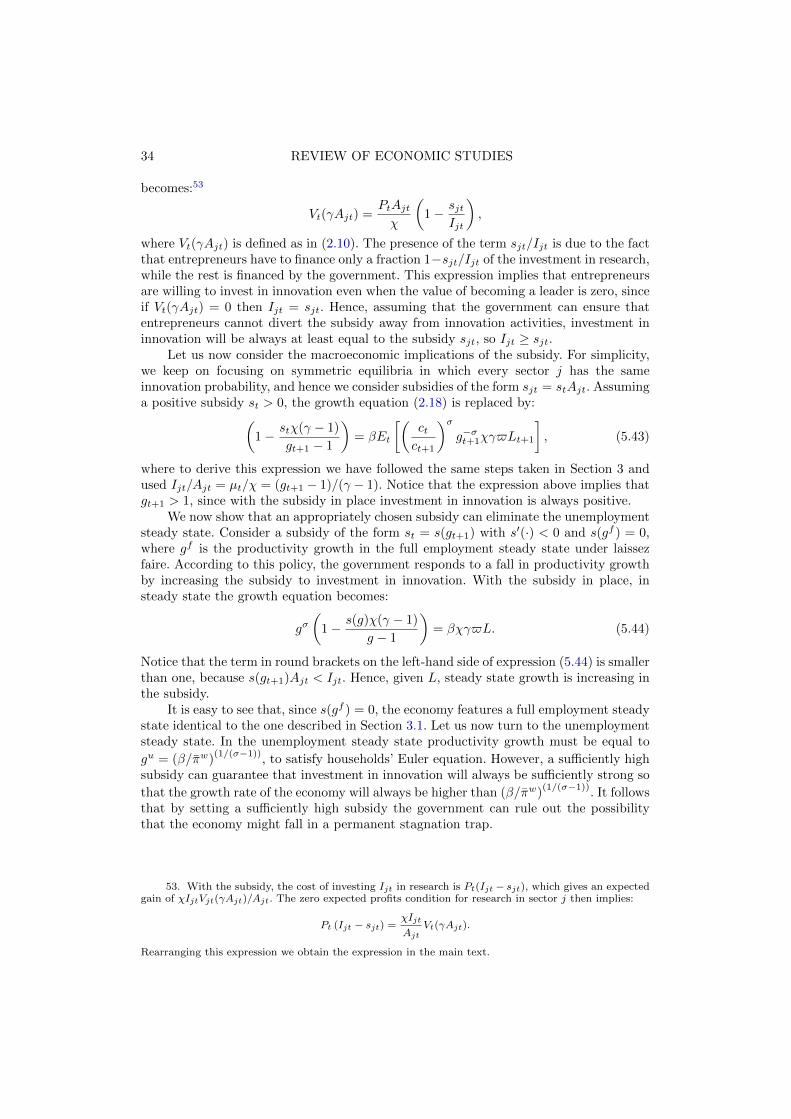
34 REVIEW OF ECONOMIC STUDIES
becomes:53
Vt(γAjt) =PtAjtχ
(1− sjt
Ijt
),
where Vt(γAjt) is defined as in (2.10). The presence of the term sjt/Ijt is due to the factthat entrepreneurs have to finance only a fraction 1−sjt/Ijt of the investment in research,while the rest is financed by the government. This expression implies that entrepreneursare willing to invest in innovation even when the value of becoming a leader is zero, sinceif Vt(γAjt) = 0 then Ijt = sjt. Hence, assuming that the government can ensure thatentrepreneurs cannot divert the subsidy away from innovation activities, investment ininnovation will be always at least equal to the subsidy sjt, so Ijt ≥ sjt.
Let us now consider the macroeconomic implications of the subsidy. For simplicity,we keep on focusing on symmetric equilibria in which every sector j has the sameinnovation probability, and hence we consider subsidies of the form sjt = stAjt. Assuminga positive subsidy st > 0, the growth equation (2.18) is replaced by:(
1− stχ(γ − 1)
gt+1 − 1
)= βEt
[(ctct+1
)σg−σt+1χγ$Lt+1
], (5.43)
where to derive this expression we have followed the same steps taken in Section 3 andused Ijt/Ajt = µt/χ = (gt+1 − 1)/(γ − 1). Notice that the expression above implies thatgt+1 > 1, since with the subsidy in place investment in innovation is always positive.
We now show that an appropriately chosen subsidy can eliminate the unemploymentsteady state. Consider a subsidy of the form st = s(gt+1) with s′(·) < 0 and s(gf ) = 0,where gf is the productivity growth in the full employment steady state under laissezfaire. According to this policy, the government responds to a fall in productivity growthby increasing the subsidy to investment in innovation. With the subsidy in place, insteady state the growth equation becomes:
gσ(
1− s(g)χ(γ − 1)
g − 1
)= βχγ$L. (5.44)
Notice that the term in round brackets on the left-hand side of expression (5.44) is smallerthan one, because s(gt+1)Ajt < Ijt. Hence, given L, steady state growth is increasing inthe subsidy.
It is easy to see that, since s(gf ) = 0, the economy features a full employment steadystate identical to the one described in Section 3.1. Let us now turn to the unemploymentsteady state. In the unemployment steady state productivity growth must be equal to
gu = (β/πw)(1/(σ−1))
, to satisfy households’ Euler equation. However, a sufficiently highsubsidy can guarantee that investment in innovation will always be sufficiently strong so
that the growth rate of the economy will always be higher than (β/πw)(1/(σ−1))
. It followsthat by setting a sufficiently high subsidy the government can rule out the possibilitythat the economy might fall in a permanent stagnation trap.
53. With the subsidy, the cost of investing Ijt in research is Pt(Ijt − sjt), which gives an expectedgain of χIjtVjt(γAjt)/Ajt. The zero expected profits condition for research in sector j then implies:
Pt (Ijt − sjt) =χIjt
AjtVt(γAjt).
Rearranging this expression we obtain the expression in the main text.
BENIGNO AND FORNARO STAGNATION TRAPS 35
Lu 1
gu
gf
gu
AD
GG
growth
g
employment L
GG laissez faireGG with growth subsidy
Lu′ Lu 1
gu
gf
gu
AD
GG
growth
g
employment L
GG laissez faireGG with growth subsidy
Figure 8Steady state with growth subsidy.
Notes: Left panel: large subsidy. Right panel: small subsidy.
Proposition 4. Suppose that there is a subsidy to innovation s(gt+1) satisfyings′(·) < 0, s(gf ) = 0 and:
1 + s
((β
πw
) 1σ−1
)χ(γ − 1) >
(β
πw
) 1σ−1
, (5.45)
and that the conditions stated in Proposition 1 hold. Then there exists a unique steadystate. The unique steady state is characterized by full employment.
Intuitively, the subsidy to innovation guarantees that even if firms’ profits were tofall substantially, investment in innovation would still be relatively high. In turn, a highinvestment in innovation stimulates growth and aggregate demand, since a high futureincome is associated with a high present demand for consumption. By implementing asufficiently high subsidy, the government can eliminate the possibility that aggregatedemand will be low enough to make the zero lower bound constraint on the nominalinterest rate bind. It is in this sense that growth policies can be thought as a tool tomanage aggregate demand in our framework. Importantly, to lift the economy out of astagnation trap the subsidy to investment has to be large enough, so as to engineer aradical regime shift in agents’ expectations about future growth.54
54. One might wonder how important it is that the subsidy is contingent on productivity growth.It turns out that totally analogous results can be obtained with a subsidy contingent on employment.Moreover, even a sufficiently large non-contingent subsidy can rule out the unemployment steady state.However, a non-contingent subsidy will also increase growth, perhaps to an inefficiently high value, inthe full employment steady state.
The results summarized in Proposition 4 readily extend, under a caveat, to the case of theeconomy with a wage Phillips curve described in Section 4.2. The caveat is that wage inflation shouldnot fall too much as employment approaches zero. Using the notation of Section 4.2, the function ψ(·)must be such that:
limL→0
ψ(L) ≥β(
gf)σ−1
.Intuitively, if this condition does not hold, even when the subsidy is sufficiently high so that productivitygrowth cannot fall below its value in the full employment steady state there still exists an 0 < L < 1consistent with a steady state in which i = 0. In this case, it is not possible to rule out the unemploymentsteady state with a subsidy that is a continuous function of productivity growth or employment. However,even when the condition above fails, it is still possible to rule out the unemployment steady state bydesigning subsidy schemes that are discontinuous functions of productivity growth or employment.
36 REVIEW OF ECONOMIC STUDIES
Graphically, the impact of the subsidy is illustrated by Figure 8. The blue solid linecorresponds to the GG curve of the economy without subsidy, while the blue dashed linerepresents the GG curve of an economy with a subsidy to investment in innovation. Thesubsidy makes the GG curve rotate up, because for a given level of employment andaggregate demand the subsidy increases the growth rate of the economy. If the subsidyis sufficiently high, as it is the case in the left panel of the figure, the unemploymentsteady state disappears and the only possible steady state is the full employment one.By contrast, the right panel of Figure 8 shows the impact of a small subsidy. A smallsubsidy makes the GG curve rotate up, but not enough to eliminate the unemploymentsteady state. In fact, the small subsidy leads to lower employment in the unemploymentsteady state compared to the laissez faire economy.
Summarizing, there is a role for well-designed subsidies to growth-enhancinginvestment, a typical supply side policy, in stimulating aggregate demand so as to ruleout liquidity traps driven by expectations of weak future growth. In turn, the stimulus toaggregate demand has a positive impact on employment. In this sense, our model helpsto rationalize the notion of job creating growth.
6. CONCLUSION
In this paper, we have presented a Keynesian growth model in which endogenousgrowth interacts with the possibility of involuntary unemployment due to weak aggregatedemand. The combination of these two factors can give rise to stagnation traps, thatis persistent liquidity traps characterized by unemployment and weak growth. All ittakes for the economy to fall into a stagnation trap is a wave of pessimism about futuregrowth. We show that policy interventions to support growth can lead the economy outof a stagnation trap, as long as they are aggressive enough to generate a regime shift inagents’ expectations about future growth .
Our analysis represents a first step toward understanding the interactions betweenbusiness cycles, growth and stagnation, and it leaves open several exciting avenues forfuture research. We conclude the paper by mentioning three of them. First, in orderto focus the analysis on fluctuations driven by shocks to expectations, in this paper wehave abstracted from fundamental shocks. Can fundamental shocks, such as productivity,monetary or news shocks, lead to prolonged periods of stagnation? Does the impact offundamental shocks on the economy depend on whether the economy is undergoing aperiod of stagnation? These are examples of questions that our model can help to answer.Second, in this paper we have focused on a subset of possible policy interventions, but itwould interesting to study other policy tools, such as fiscal policy. Third, in this paperwe have abstracted from financial frictions. However, it is easy to imagine a channelthrough which growth and aggregate demand can interact when firms’ access to financingis limited. In fact, if access to credit is tight, firms’ investment in innovation will beconstrained by their internal funds. In turn, a period of low aggregate demand and weakprofits will erode firms’ internal funds, and thus their ability to invest in productivity-enhancing activities. Through this channel, a period of low aggregate demand will leadto low productivity growth. Indeed, we conjecture that economies undergoing a period offinancial stress might be particularly exposed to the risk of expectation-driven stagnationtraps. This might contribute to explain why the episodes of stagnation affecting Japan,the US and the Euro area coincided, at least in their beginning, with periods of tightaccess to credit.
BENIGNO AND FORNARO STAGNATION TRAPS 37
APPENDIX A. PROOFS
Appendix A.1. Proof of Proposition 1 (existence, uniqueness and local determinacy of fullemployment steady state)
Proof. We start by proving existence. A steady state is described by the system (3.21)-(3.24).Setting L = 1 and using the first inequality in condition (3.29), equation (3.22) implies:
gf = (βχγ$)1σ . (A46)
Condition (3.29) implies 1 < gf < γ. Then equation (3.21) implies:
1 + if =πw(gf)σ−1
β. (A47)
Assumption (3.27) guarantees that if > 0 and i = if , so that the interest rate rule (3.24) is compatiblewith the existence of a full employment steady state. Moreover, combining equations (3.22) and (3.23)
evaluated at L = 1 and g = gf gives:
cf = Ψ−gf − 1
χ(γ − 1). (A48)
One can check that the second inequality in condition (3.29) ensures that cf > 0. Hence, a full
employment steady state exists.
To prove uniqueness, consider that equation (A46) implies that there is only one value of g
consistent with the full employment steady state, while equation (A47) establishes that there is a uniquevalue of i consistent with g = gf . Hence, the full employment steady state is unique.
We now show that the full employment steady state is locally determinate. A loglinear
approximation of equations (2.17)− (2.20) around the full employment steady state gives:
(σ − 1)gt+1 = it + σ(ct − Et[ct+1]) (A49)
Lt =cf
Ψct +
(1−
cf
Ψ
)gf
gf − 1gt+1 (A50)
σgt+1 = σ(ct − Et[ct+1]) + Et[Lt+1
](A51)
it = φLt, (A52)
where x ≡ log(xt)− log(xf ) for every variable x, except for gt ≡ gt − gf and i ≡ it − i, while Ψ is GDPnormalized by the productivity index. This system can be written as:
Lt = ξ1Et[Lt+1] + ξ2Et[gt+2] (A53)
gt+1 = ξ3Et[Lt+1] + ξ4Et[gt+2], (A54)
where
ξ1 ≡Ψcf− 1σ
+(
1 + Ψ−cfcf
gf
gf−1
)Ψcf
+ φ(
1 + Ψ−cfcf
gf
gf−1
)
ξ2 ≡ −Ψ−cfcf
gf
gf−1
Ψcf
+ φ(
1 + Ψ−cfcf
gf
gf−1
)ξ3 ≡ 1− φξ1
ξ4 ≡ −φξ2.The system is determinate if and only if:55
|ξ1ξ4 − ξ2ξ3| < 1 (A55)
|ξ1 + ξ4| < 1 + ξ1ξ4 − ξ2ξ3. (A56)
55. See Bullard and Mitra (2002).
38 REVIEW OF ECONOMIC STUDIES
Condition (A55) holds if:
φ >
Ψ−cfΨ
gf
gf−1− 1
cf
Ψ+ Ψ−cf
Ψgf
gf−1
, (A57)
while condition (A56) holds if:
φ > 1−1
σ. (A58)
Assumption (3.28) guarantees that (A56) holds. Moreover, using (A48), after some algebra, condition
(A57) can be written as:
(1 + φ)Ψ +φ− gf
χ(γ − 1)> 0.
By condition (3.29) the inequality above is true if:
φ > 1/gf = 1/(βχγ$)1/σ ,
which holds by assumption (3.28). Hence, (A55) holds and the full employment steady state is locallydeterminate.
Appendix A.2. Proof of Proposition 2 (existence, uniqueness and local indeterminacy ofunemployment steady state)
Proof. We start by showing that it is not possible to have an unemployment steady state with apositive nominal interest rate. Suppose that this is not the case, and that there is a steady state with
1 + i = (1 + i)Lφ and 0 ≤ L < 1. Then combining equations (3.21) and (3.22), and using βχγ$ = gf
and 1 + i =(gf)σ−1
πw/β gives:
gfLφσ−1 =
(max
((gf)σ
L, 1)) 1
σ. (A59)
Assumption (3.28) implies that the left-hand side of this expression is smaller than the right-hand side
for any 0 ≤ L < 1. Hence, we have found a contradiction and an unemployment steady state with i > 0
is not possible.
We now prove that an unemployment steady state with i = 0 exists and is unique. Setting i = 0,
equation (3.21) implies that there is a unique value of g = (β/πw)1/(σ−1) = gu consistent with theunemployment steady state. Moreover, since if > 0 equation (3.21) also implies that gu < gf , while the
first inequality in condition (3.30) implies gu > 1. Evaluating equation (3.22) at g = gu we have:
Lu =(gu)σ
βχγ$,
ensuring that there is a unique value of L = Lu > 0 consistent with g = gu. Moreover, using gu < gf
and equation (3.22) gives Lu < 1. Combining equations (3.22) and (3.23) evaluated at L = Lu and
g = gu, one can check that the second inequality in condition (3.30) ensures that cu > 0. Hence, the
unemployment steady state exists and is unique. Finally, using if > 0 and gu < gf one can see that1/πu = gu/πw < (1+ if )gf/πw = (1+ if )/πf , so that the real interest rate in the unemployment steadystate is lower than the one in the full employment steady state.
To prove local indeterminacy one can follow the steps of the proof to proposition one. Since in theneighborhood of the unemployment steady state it = 0, it is easy to show that condition (A56) cannot
be satisfied.
Appendix A.3. Proof of Proposition 3 (optimal discretionary monetary policy)
Proof. Under discretion, every period the central bank maximizes the representative householdexpected utility subject to (2.17), (2.18), (2.19), Lt ≤ 1 and it ≥ 0, taking future variables as given. The
central bank’s problem can be written as:
maxLt,ct,gt+1,it
Et
∞∑τ=t
βτ
(C1−στ − 1
1− σ
= Et
[βtA1−σ
t
(c1−σt
1− σ+ gt+1ν
1t
)]−
1
(1− β)(1− σ),
BENIGNO AND FORNARO STAGNATION TRAPS 39
subject to:
Lt =1
Ψ
(ct +
gt+1 − 1
χ(γ − 1)
)
ct =
(gσ−1t+1
1 + it
) 1σ
ν2t
gt+1 = max
(1,
ν3t
1 + it
)Lt ≤ 1
it ≥ 0,
where the third constraint is obtained by combining (2.17) and (2.18), and:
ν1t = Et
∞∑τ=t+1
βτ
(cτΠττ=t+2gτ
)1−σ
1− σ
ν2t =
πw
βEt[c−σt+1
] 1σ
ν3t = πwχγ$
Et[Lt+1c−σt+1]
Et[c−σt+1]
.
ν1t , ν2
t and ν3t are taken as given by the central bank, because they are function of parameters and
expectations about future variables only.
Notice that the objective function is strictly increasing in ct and gt+1. Also notice that from thesecond and third constraints we can write ct = c(it) with c′(it) < 0 and gt+1 = g(it) with g′(it) ≤ 0.
We can then rewrite the problem of a central bank under discretion as
min it,
subject to:
Lt =1
Ψ
(c(it) +
g(it)− 1
χ(γ − 1)
)Lt ≤ 1
it ≥ 0.
The solution to this problem can be expressed by the complementary slackness condition:
it (Lt − 1) = 0.
Appendix A.4. Proof of Proposition 4 (uniqueness of steady state with subsidy to innovation)
The proof that a full employment steady state exists and is unique follows the steps of the proof to
Proposition 1.
We now prove that there is no steady state with unemployment. Following the proof to proposition2, one can check that if another steady state exists, it must be characterized by i = 0. Equation (2.17)
implies that in this steady state growth must be equal to (β/πw)(1/(σ−1)). Suppose that a steady statewith g = (β/πw)(1/(σ−1)) exists. Then equation (5.44) implies that there must be an 0 ≤ L ≤ 1 suchthat:
L =
(β
πw
) σσ−1
1−s
((βπw
) 1σ−1
)χ(γ − 1)(
βπw
) 1σ−1 − 1
(βχγ$)−1.
40 REVIEW OF ECONOMIC STUDIES
But condition (5.45) implies L < 0, a contradiction. Hence, an unemployment steady state does notexist. �
APPENDIX B. MODEL WITH MONEY
In this appendix we explicitly introduce money in the model. The presence of money rationalizes the
zero lower bound constraint on the nominal interest rate, but does not alter the equilibrium conditions
of the model.Following Krugman (1998) and Eggertsson (2008) we assume that households need to hold at least
a fraction ν > 0 of production in money balances M :
Mt ≥ νPtYt. (B60)
The household’s budget constraint is now:
PtCt +bt+1
1 + it+Mt = WtLt + bt +Mt−1 + dt − Tt, (B61)
where Mt denotes money holdings at time t to be carried over at time t+ 1, and T are lump-sum taxespaid to the government.
The optimality condition with respect to Mt is:
λt = βEt [λt+1] + µt, (B62)
where µt > 0 is the Lagrange multiplier on constraint (B60). Combining optimality conditions (2.3) and
(B62) it is easy to see that the presence of money implies it ≥ 0. Intuitively, households will always
prefer to hold money, rather than an asset which pays a non-contingent negative nominal return. It isalso easy to see that constraint (B60) binds if it > 0, but it is slack if it = 0. Hence, households’ money
demand is captured by the complementary slackness condition:
it
(Mt − νPt
(α
ξ
) α1−α
AtLt
)= 0, (B63)
with it ≥ 0 and Mt ≥ νPt(αξ
) α1−α
AtLt, where we have substituted Yt using equation (2.9).
To close the model, we assume that the government runs a balanced budget:
Tt = Mt −Mt−1,
so that seignorage revenue is rebated to households via lump sum taxes.We can now define an equilibrium as a set of processes {Lt, ct, gt+1, it,Mt, Pt}+∞t=0 satisfying
equations (2.17)− (2.20), (B63) and Pt = πwPt−1/gt, given initial values P−1, A0.56
Notice that to solve for the path of Lt, ct, gt+1 and it only equations (2.17)− (2.20) are needed.Given values for Lt, At and Pt, the only use of the money demand equation (B63) is to define the
money supply Mt consistent with the central bank’s interest rate rule. Specifically, when it > 0
the equilibrium money supply is Mt = νPt (α/ξ)α
1−α AtLt, while when it = 0 any money supply
Mt ≥ νPt (α/ξ)α
1−α AtLt is consistent with equilibrium.These results do not rest on the specific source of money demand assumed. For instance, similar
results can be derived in a setting in which households derive utility from holding real money balances,
as long as a cashless limit is considered (Eggertsson and Woodford, 2003).
APPENDIX C. THE CASES OF σ = 1 AND σ < 1
In the main text we have focused attention on the empirically relevant case of low elasticity ofintertemporal substitution, by assuming that σ > 1. In this appendix we consider the alternative casesσ = 1 and σ < 1. The key result is that under these cases the steady state is unique.
We start by analyzing the case of σ = 1. In steady state, equation (3.21) can be written as:
1 =β(1 + i)
πw.
56. To derive the law of motion for Pt we have used the equilibrium condition πt = πwt /gt and thelaw of motion for Wt.
BENIGNO AND FORNARO STAGNATION TRAPS 41
Intuitively, under this case changes in the growth rate of the economy have no impact on the equilibriumnominal interest rate. Hence, if there exists a full employment equilibrium featuring a positive nominal
interest rate, it is easy to check that no unemployment equilibrium can exist.
We now turn to the case σ < 1. Under this case, equation (3.21) implies a negative relationshipbetween growth and the nominal interest rate. Supposing that a full employment equilibrium featuring
a positive nominal interest rate exists, if a liquidity trap equilibrium exists, it must feature a higher
growth rate than the full employment one, i.e. gu > gf . Since Lf = 1, it must be the case that Lu ≤ Lf .But equation (3.22) implies a nonnegative steady state relationship between g and L. Then we cannot
have a steady state in which gu > gf and Lu ≤ Lf , so that, if the economy features a full employment
steady state, an unemployment steady state cannot exist.
APPENDIX D. NUMERICAL SOLUTION METHOD TO COMPUTE PERFECTFORESIGHT TRANSITIONS
The objective is to compute a sequence {gt+1, Lt, ct, it}Tt=0 given an initial condition L0 for T large suchthat:
cσt =cσt+1g
σ−1t+1 π
w
β(1 + it)(D64)
(gt+1 − 1)
(1− β
[(ct
ct+1
)σg−σt+1χγ$Lt+1
])= 0 (D65)
ct = ΨLt −gt+1 − 1
χ(γ − 1)(D66)
1 + it = max(
(1 + i)Lφt , 1), (D67)
and Lt ≤ 1 hold for all t ∈ {0, ..., T}. We restrict attention to sequences that converge to the
unemployment steady state.
The algorithm follows these steps:
1 Guess a sequence {Lt}T+1t=1 . Set LT+1 = Lu.
2 Use (D64), (D65), (D66) and (D67) evaluated at t = 0, the initial condition L0 and the guess forL1 to solve for g1 and c0.
3 For any t ∈ {1, ..., T}, use equations (D64) and (D67) evaluated at t− 1 and values for Lt−1, gtand ct−1 to solve for ct. Use (D64), (D65), (D66) and (D67) evaluated at t, and Lt+1 to solvefor gt+1.
4 Use equations (D64) and (D67) evaluated at T and values for LT , gT+1 and cT to solve for cT+1.5 Evaluate convergence by checking that the market clearing condition (D66) holds for any
t ∈ {1, ..., T} and that the sequence has converged to the unemployment steady state. Ifsup ||ΨLt − ct − (gt+1 − 1)(χ(γ − 1))|| for all t ∈ {1, ..., T} and ||cT+1 − cu|| are sufficiently
small we have found a solution. Otherwise compute:
Lt = Lt − ε(
ΨLt − ct −gt+1 − 1
χ(γ − 1)
),
where ε is a small positive number. Update the guess by setting Lt = min(Lt, 1
)for any
t ∈ {1, ..., T} and go to step 2.
APPENDIX E. MODEL WITH UNEMPLOYMENT RISK
In this appendix, we lay down the model with idiosyncratic unemployment risk described in Section 4.1.
In this model, each household faces in every period a constant probability p of being unemployed. The
employment status is revealed to the household at the start of the period. An unemployed householdreceives an unemployment benefit, such that its income is equal to a fraction b < 1 of the income received
by employed households. Unemployment benefits are financed with taxes on employed households.
The budget constraint of a household now becomes:
PtCt +bt+1
1 + it= νtWtLt + bt + dt + Tt.
42 REVIEW OF ECONOMIC STUDIES
The only change with respect to the benchmark model is the presence of the variables ν and T , whichsummarize the impact of the employment status on a household’s budget. ν is an indicator variable
that takes value 1 if the household is employed, and 0 if the household is unemployed. T represents a
lump-sum transfer for unemployed households, and a tax for employed households. T is set such that theincome of an unemployed household is equal to a fraction b of the income of an employed household.57
Moreover, here we assume that households cannot borrow:
bt+1 ≥ 0,
and that trade in firms’ shares is not possible, so that every household receives the same dividends d.
The Euler equation is now:
c−σt =β(1 + it)Et
[c−σt+1
]gσ−1t+1 π
w+ µt,
where µt is the Lagrange multiplier on the borrowing constraint and, as in the main text, ct ≡ Ct/At.We start by showing that the borrowing constraint binds only for unemployed households. Since
neither households nor firms can borrow, in equilibrium every period every household consumes her
entire income. Denoting, by cet and cnet the consumption of respectively an employed and an unemployedhousehold, we have cnet = bcet < cet . Moreover, due to the assumption of i.i.d. idiosyncratic shocks,
Et[c−σt+1
]is independent of the employment status. Hence, from the Euler equation it follows that
µt > 0 only for the unemployed, and so the borrowing constraint does not bind for employed households.
The Euler equation of the employed households is:
(cet )σ =
πwgσ−1t+1
β(1 + it)ρEt
[(cet+1
)−σ] ,where ρ ≡ 1− p+ p/bσ > 1, and we have used the fact that the probability of becoming unemployed isindependent of aggregate shocks. Moreover, using ct = pcnet + (1− p)cet = cet (bp+ 1− p), we obtain:
cσt =πgσ−1t+1
β(1 + it)ρEt[c−σt+1
] .This equation, which is the equivalent of equation (2.17) in the baseline model, determines the demand
for consumption in the model with idiosyncratic unemployment risk.
APPENDIX F. ALTERNATIVE GROWTH PROCESSES
Appendix F.1. Innovation by incumbents
In our baseline model, as in Aghion and Howitt (1992) and Grossman and Helpman (1991), all the
innovation is performed by entrants. However, in the data most quality improvements of existing products
seem the result of investment by incumbent firms, and the contribution of incumbents to productivitygrowth is substantial (Bartelsman and Doms, 2000). Motivated by these facts, in this appendix we
describe a model in which innovation is carried out by incumbent firms. As in chapter 7 of Barro and
Sala-i Martin (2004), incumbents end up investing in innovation because they enjoy a cost advantage inresearch with respect to entrants.
57. More precisely, an unemployed household receives a transfer:
T =bWtLt + (b− 1)dt
1 + bp1−p
,
while an employed household pays a tax
T = −p
1− pbWtLt + (b− 1)dt
1 + bp1−p
.
BENIGNO AND FORNARO STAGNATION TRAPS 43
In line with the baseline model, we assume that an incumbent in a generic sector j that invests Ijtunits of the final good to discover an improved version of product j innovates with probability:
µjt = min
(χIIjt
Ajt, 1
).
We follow Barro and Sala-i Martin (2004) and assume that χI , the parameter capturing incumbents’
productivity in research, is sufficiently larger than χ, the parameter capturing outsiders’ productivity in
research, so that all the innovation activities are carried out by incumbents.
The flow of monopoly profit enjoyed by an incumbent with productivity Ajt is still given by
Pt$AjtLt.58 The end-of-period value associated with being an incumbent with productivity Ajt is thus
given by:
V It (Ajt) = βρEt
[λt+1
λt
(Pt+1$AjtLt+1 + (1− η)
(µj,t+1V
It+1(γAjt) + (1− µj,t+1)V It+1(Ajt)− Pt+1Ij,t+1
))].
(F68)
The first term inside the parenthesis on the right-hand side, also present in the baseline model, captures
the expected profits to be gained in period t+1. The second term captures the incumbent’s continuationvalue in period t + 1. With probability 1 − η the firm survives.59 In period t + 1 the firm makes a
new discovery with probability µj,t+1, in which case its value is given by V It+1(γAjt). Instead, with
probability 1−µj,t+1 no innovation occurs in period t+ 1, and the continuation value is V It+1(Ajt). The
term Pt+1Ij,t+1 captures the cost of the investment in innovation performed by the firm in period t+ 1.The expected profits are discounted using the households’ discount factor βρEt [λt+1/λt].
We now derive the equilibrium in the market for innovation. The expected return that an incumbent
receives from investing Ijt in research is given by
χIIjt
Ajt
(V It (γAjt)− V It (Aj,t)
)− PtIjt. (F69)
This expression captures the fact that the incumbent captures only the increment in present value
from innovation, V It (γAjt) − V It (Aj,t), because the incumbent does not value the expropriation of its
own monopoly profits. We focus on equilibria in which investment in innovation is positive and finite.Differentiating the previous expression with respect to Ijt, this requires that
Pt =χI
Ajt
(V It (γAjt)− V It (Aj,t)
),
so that in equilibrium the innovation costs are equal to the expected gains. Moreover, we focus on
symmetric equilibria in which V It (Ajt) = V It Ajt for every j. Plugging this condition in expression (F69)implies that in equilibrium V It = Pt/((γ − 1)χI). We can thus write expression (F68) as:
Pt
χI= βρEt
[λt+1
λt
(Pt+1$(γ − 1)Lt+1 + (1− η)
Pt+1
χI
)].
This expression summarizes the equilibrium in the research sector. Combining this expression with
equation (2.2) gives:
gσt+1 = βρEt
[(ct
ct+1
)σ (χI(γ − 1)$Lt+1 + 1− η
)],
which replaces equation (2.18) of the baseline model.
Appendix F.2. Productivity spillovers across firms
In this appendix we lay down a version of the model in which the profits of non-innovating firm partlydepend on aggregate productivity growth. For instance, this is the case in Grossman and Helpman (1991),in which profits are the same across all the firms and grow at the rate of aggregate productivity growth.
58. Since there are no competitors, however, each incumbent sets the unconstrained markup andso ξ = 1/α.
59. As in the model with innovation by entrants, we assume that every period there is a constantprobability η that the incumbent firm dies and is replaced by another firm that inherits its technology.
44 REVIEW OF ECONOMIC STUDIES
To implement this idea, we assume that the production function of the final good is:
Yt = L1−αt
∫ 1
0
(A1−θt Aθjt
)1−αxαjtdj, where At ≡
(∫ 1
0Aθjtdj
) 1θ
, (F70)
where 0 < θ ≤ 1. When θ < 1, this production function implies that the productivity of an intermediate
input is increasing in aggregate productivity, capturing the notion of productivity spillovers across firms.
Instead, the case θ = 1 corresponds to our baseline model in which spillovers are absent.
Following the same steps used to solve the baseline model, it is easy to show that under this
production function aggregate output is given by:
Yt =
(α
ξ
) α1−α
AtLt, (F71)
while the profits of an incumbent firm in a generic sector j are equal to:
Pt$A1−θt AθjtLt. (F72)
Hence, when θ < 1 an increase in aggregate productivity generates a rise in profits for all firms. This
implies that the profits of non-innovating firms grow at rate g1−θt . It is also easy to check that aggregate
productivity growth is given by:
gt+1 =(µt(γ
θ − 1) + 1) 1θ, (F73)
where µt is the fraction of innovating sectors.
It is possible to embed this production function both in the model with innovation by entrants or
incumbents. For concreteness, we focus on the latter case. As in the baseline model, we assume that thecost of innovation is proportional to the productivity of the intermediate input A1−θ
t Aθjt:
µjt = min
(χIIjt
A1−θt Aθjt
, 1
),
The growth equation in this version of the model, which can be derived following the steps outlined in
Section AppendixF.1, is given by:
gσ−(1−θ)t+1 = βρEt
[(ct
ct+1
)σ (χI(γ − 1)$Lt+1 + 1− η
)],
which replaces equation (2.18) of the baseline model.
APPENDIX G. DATA APPENDIX
This appendix provides details on the construction of the series underlying Table 1.
1 Policy rate. Central bank discount rate. Monthly series from the IMF International Financial
Statistics database.
2 Unemployment rate. Annual series from the IMF International Financial Statistics database.
3 Labor productivity. Real GDP divided by total hours worked. Annual data from the ConferenceBoard Total Economy Database. The Euro area is defined as the aggregate of Austria, Belgium,
Finland, Germany, Greece, Ireland, Italy, Netherlands, Portugal and Spain.
4 R&D intensity. R&D intensity is the ratio of investment in R&D to R&D stock for the business
sector. We use this measure of investment in R&D for two reasons. First, this is the variablethat determines the growth rate of productivity in our model, as well as in the seminal growthframeworks developed by Aghion and Howitt (1992), Grossman and Helpman (1991) and Romer
(1990). Second, Kung and Schmid (2015), using US data for the period 1953-2008, show that thisvariable predicts productivity, output and consumption growth at horizons of one to five years.
Figure 9 shows the research intensity series underlying the numbers in Table 1.
Formally, R&D intensity is defined as RDinv,t/RDstock,t, where RDinv,t is investment in R&Dby the business sector during period t, while RDstock,t is the stock of business R&D at the start
of period t. We construct a measure of the business sector R&D stock in accordance with the
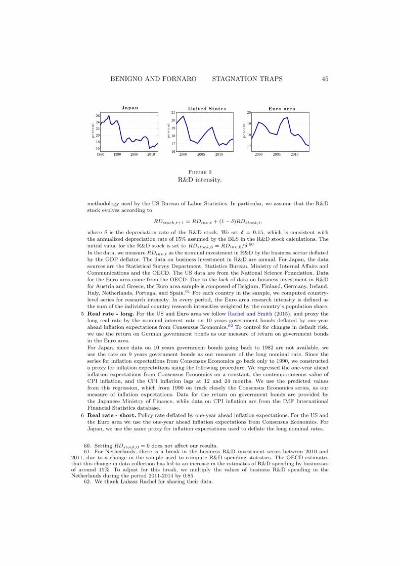
BENIGNO AND FORNARO STAGNATION TRAPS 45
1980 1990 2000 2010
16
18
20
22
24
26
Japan
percent
2000 2005 201016
17
18
19
20
21United States
percent
2000 2005 2010
17
18
19
20Euro area
percent
Figure 9
R&D intensity.
methodology used by the US Bureau of Labor Statistics. In particular, we assume that the R&D
stock evolves according to
RDstock,t+1 = RDinv,t + (1− δ)RDstock,t,
where δ is the depreciation rate of the R&D stock. We set δ = 0.15, which is consistent with
the annualized depreciation rate of 15% assumed by the BLS in the R&D stock calculations. Theinitial value for the R&D stock is set to RDstock,0 = RDinv,0/δ.
60
In the data, we measure RDinv,t as the nominal investment in R&D by the business sector deflatedby the GDP deflator. The data on business investment in R&D are annual. For Japan, the data
sources are the Statistical Survey Department, Statistics Bureau, Ministry of Internal Affairs and
Communications and the OECD. The US data are from the National Science Foundation. Datafor the Euro area come from the OECD. Due to the lack of data on business investment in R&D
for Austria and Greece, the Euro area sample is composed of Belgium, Finland, Germany, Ireland,
Italy, Netherlands, Portugal and Spain.61 For each country in the sample, we computed country-level series for research intensity. In every period, the Euro area research intensity is defined as
the sum of the individual country research intensities weighted by the country’s population share.
5 Real rate - long. For the US and Euro area we follow Rachel and Smith (2015), and proxy the
long real rate by the nominal interest rate on 10 years government bonds deflated by one-yearahead inflation expectations from Consensus Economics.62 To control for changes in default risk,
we use the return on German government bonds as our measure of return on government bonds
in the Euro area.
For Japan, since data on 10 years government bonds going back to 1982 are not available, we
use the rate on 9 years government bonds as our measure of the long nominal rate. Since theseries for inflation expectations from Consensus Economics go back only to 1990, we constructed
a proxy for inflation expectations using the following procedure. We regressed the one-year ahead
inflation expectations from Consensus Economics on a constant, the contemporaneous value ofCPI inflation, and the CPI inflation lags at 12 and 24 months. We use the predicted values
from this regression, which from 1990 on track closely the Consensus Economics series, as ourmeasure of inflation expectations. Data for the return on government bonds are provided bythe Japanese Ministry of Finance, while data on CPI inflation are from the IMF InternationalFinancial Statistics database.
6 Real rate - short. Policy rate deflated by one-year ahead inflation expectations. For the US and
the Euro area we use the one-year ahead inflation expectations from Consensus Economics. ForJapan, we use the same proxy for inflation expectations used to deflate the long nominal rates.
60. Setting RDstock,0 = 0 does not affect our results.61. For Netherlands, there is a break in the business R&D investment series between 2010 and
2011, due to a change in the sample used to compute R&D spending statistics. The OECD estimatesthat this change in data collection has led to an increase in the estimates of R&D spending by businessesof around 15%. To adjust for this break, we multiply the values of business R&D spending in theNetherlands during the period 2011-2014 by 0.85.
62. We thank Lukasz Rachel for sharing their data.

46 REVIEW OF ECONOMIC STUDIES
Acknowledgements. We thank the Editor, Gita Gopinath, four anonymous referees, PhilippeAghion, Pierpaolo Benigno, Javier Bianchi, Seonghoon Cho, Roger Farmer, Andrea Ferrero, Jordi Gali,
Jang-Ting Guo, Bob Hall, Chad Jones, Nobuhiro Kiyotaki, Robert Kollmann, Tommaso Monacelli,
Jaume Ventura, Alwyn Young, and participants at several seminars and conferences for useful comments.We are grateful to Julia Faltermeier, Andresa Lagerborg, Youel Rojas and Martin Wolf for excellent
research assistance. This research has been supported by the ESRC grant ES/I024174/1, the Spanish
Ministry of Science and Innovation (grant ECO2011-23192), the Fondation Banque de France ResearchGrant, the CERCA Programme/Generalitat de Catalunya and the Spanish Ministry of Economy and
Competitiveness, through the Severo Ochoa Programme for Centres of Excellence in RD (SEV-2015-
0563). The contribution by Luca Fornaro to this paper has been prepared under the LamfalussyFellowship Program sponsored by the European Central Bank. Any views expressed are only those
of the authors and do not necessarily represent the views of the ECB or the Eurosystem.
REFERENCES
Acemoglu, D., P. Aghion, L. Bursztyn, and D. Hemous (2012). The environment and directed technical
change. American Economic Review 102 (1), 131–166.Acemoglu, D. and U. Akcigit (2012). Intellectual property rights policy, competition and innovation.
Journal of the European Economic Association 10 (1), 1–42.Acemoglu, D. and J. Linn (2004). Market size in innovation: theory and evidence from the pharmaceutical
industry. Quarterly Journal of Economics 119 (3), 1049–1090.Aghion, P., G.-M. Angeletos, A. Banerjee, and K. Manova (2010). Volatility and growth: Credit
constraints and the composition of investment. Journal of Monetary Economics 57 (3), 246–265.Aghion, P., P. Bacchetta, R. Ranciere, and K. Rogoff (2009). Exchange rate volatility and productivity
growth: The role of financial development. Journal of Monetary Economics 56 (4), 494–513.Aghion, P., C. Harris, P. Howitt, and J. Vickers (2001). Competition, imitation and growth with step-
by-step innovation. Review of Economic Studies 68 (3), 467–492.Aghion, P., D. Hemous, and E. Kharroubi (2014). Cyclical fiscal policy, credit constraints, and industry
growth. Journal of Monetary Economics 62, 41–58.Aghion, P. and P. Howitt (1992). A model of growth through creative destruction. Econometrica 60 (2),
323–351.Aghion, P. and P. Howitt (2009). The Economics of Growth. MIT Press.Akerlof, G. A., W. T. Dickens, and G. L. Perry (1996). The macroeconomics of low inflation. Brookings
Papers on Economic Activity 1996 (1), 1–76.Anzoategui, D., D. Comin, M. Gertler, and J. Martinez (2015). Endogenous technology adoption and
r&d as sources of business cycle persistence. New York University working paper.Asriyan, V., L. Fornaro, A. Martin, and J. Ventura (2016). Monetary policy for a bubbly world. CREI
working paper.Barattieri, A., S. Basu, and P. Gottschalk (2014). Some evidence on the importance of sticky wages.
American Economic Journal: Macroeconomics 6 (1), 70–101.Barlevy, G. (2007). On the cyclicality of research and development. American Economic Review 97 (4),
1131–1164.Barro, R. J. and X. Sala-i Martin (2004). Economic Growth (2nd ed.). MIT Press.Bartelsman, E. J. and M. Doms (2000). Understanding productivity: Lessons from longitudinal
microdata. Journal of Economic Literature 38 (3), 569–594.Benhabib, J. and R. E. Farmer (1994). Indeterminacy and increasing returns. Journal of Economic
Theory 63 (1), 19–41.Benhabib, J., S. Schmitt-Grohe, and M. Uribe (2001). The perils of taylor rules. Journal of Economic
Theory 96 (1), 40–69.Best, M. C., J. Cloyne, E. Ilzetzki, and H. J. Kleven (2015). Interest rates, debt and intertemporal
allocation: Evidence from notched mortgage contracts in the united kingdom. Bank of Englandworking paper.
Bianchi, F., H. Kung, and G. Morales (2015). Growth, slowdowns, and recoveries. LBS working paper.Blanchard, O., G. Lorenzoni, and J. L’Huillier (2017). Short-run effects of lower productivity growth. a
twist on the secular stagnation hypothesis. NBER Working Paper No. 23160.Bullard, J. and K. Mitra (2002). Learning about monetary policy rules. Journal of Monetary
Economics 49 (6), 1105–1129.Bussiere, M., L. Ferrara, and J. Milovich (2015). Explaining the recent slump in investment: the role of
expected demand and uncertainty. Banque de France working paper.

BENIGNO AND FORNARO STAGNATION TRAPS 47
Bustos, P. (2011). Trade liberalization, exports, and technology upgrading: Evidence on the impact ofmercosur on argentinian firms. American Economic Review 101 (1), 304–340.
Caballero, R. J. and E. Farhi (2017). The safety trap. Review of Economic Studies, forthcoming.
Caballero, R. J., E. Farhi, and P.-O. Gourinchas (2015). Global imbalances and currency wars at the
zlb. NBER Working Paper No. 21670.
CBO (2017). The budget and economic outlook: 2017 to 2027.
Comin, D. and M. Gertler (2006). Medium-term business cycles. American Economic Review 96 (3),
523–551.
Corrado, C., J. Haskel, C. Jona-Lasinio, and M. Iommi (2016). Intangible investment in the eu and us
before and since the great recession and its contribution to productivity growth. EIB Working Papers.
Del Negro, M., M. P. Giannoni, and F. Schorfheide (2015). Inflation in the great recession and new
keynesian models. American Economic Journal: Macroeconomics 7 (1), 168–196.
Eggertsson, G. and P. Krugman (2012). Debt, deleveraging, and the liquidity trap: a fisher-minsky-koo
approach. Quarterly Journal of Economics 127 (3), 1469–1513.
Eggertsson, G. and N. Mehrotra (2014). A model of secular stagnation. Brown University working paper.
Eggertsson, G., N. Mehrotra, and J. Robbins (2017). A model of secular stagnation: Theory andquantitative evaluation. NBER Working Paper No. 23093.
Eggertsson, G., N. Mehrotra, S. Singh, and L. Summers (2016). A contagious malady? open economy
dimensions of secular stagnation. NBER Working Paper No. 22299.
Eggertsson, G. and M. Woodford (2003). The zero bound on interest rates and optimal monetary policy.
Brookings Papers on Economic Activity 2003 (1), 139–211.
Eggertsson, G. B. (2008). Great expectations and the end of the depression. American Economic
Review 98 (4), 1476–1516.
Eggertsson, G. B. (2010). The paradox of toil. FRB of New York Staff Report (433).
Erceg, C. J., D. W. Henderson, and A. T. Levin (2000). Optimal monetary policy with staggered wageand price contracts. Journal of Monetary Economics 46 (2), 281–313.
Fabiani, S., C. Kwapil, T. Room, K. Galuscak, and A. Lamo (2010). Wage rigidities and labor market
adjustment in europe. Journal of the European Economic Association 8 (2-3), 497–505.
Farmer, R. E. (2012). Confidence, crashes and animal spirits. Economic Journal 122 (559), 155–172.
Fatas, A. (2000). Do business cycles cast long shadows? short-run persistence and economic growth.
Journal of Economic Growth 5 (2), 147–162.
Fehr, E. and L. Goette (2005). Robustness and real consequences of nominal wage rigidity. Journal ofMonetary Economics 52 (4), 779–804.
Galı, J. (2009). Monetary Policy, Inflation, and the Business Cycle: An Introduction to the NewKeynesian Framework. Princeton University Press.
Garcia-Macia, D. (2015). The financing of ideas and the great deviation. manuscript.
Geanakoplos, J. D. and H. M. Polemarchakis (1986). Walrasian indeterminacy and keynesian
macroeconomics. Review of Economic Studies 53 (5), 755–779.
Gottschalk, P. (2005). Downward nominal-wage flexibility: Real or measurement error? Review of
Economics and Statistics 87 (3), 556–568.
Grossman, G. M. and E. Helpman (1991). Quality ladders in the theory of growth. Review of Economic
Studies 58 (1), 43–61.
Guerrieri, V. and G. Lorenzoni (2017). Credit crises, precautionary savings, and the liquidity trap.Quarterly Journal of Economics 132 (1), 1427–1467.
Hall, R. E. (1988). Intertemporal substitution in consumption. Journal of Political Economy 96 (2),339–357.
Hall, R. E. and P. R. Milgrom (2008). The limited influence of unemployment on the wage bargain.American Economic Review 98 (4), 1653–1674.
Hansen, A. H. (1939). Economic progress and declining population growth. American Economic
Review 29 (1), 1–15.
Hausman, J. K. and J. F. Wieland (2014). Abenomics: preliminary analysis and outlook. Brookings
Papers on Economic Activity 2014 (1), 1–63.
Havranek, T. (2015). Measuring intertemporal substitution: The importance of method choices andselective reporting. Journal of the European Economic Association 13 (6), 1180–1204.
Howitt, P. (2000). Endogenous growth and cross-country income differences. American EconomicReview 90 (4), 829–846.
Howitt, P. and P. Aghion (1998). Capital accumulation and innovation as complementary factors in
long-run growth. Journal of Economic Growth 3 (2), 111–130.

48 REVIEW OF ECONOMIC STUDIES
Huggett, M. (1993). The risk-free rate in heterogeneous-agent incomplete-insurance economies. Journalof Economic Dynamics and Control 17 (5-6), 953–969.
IMF (2015, April). Private investment: What’s the holdup? IMF World Economic Outlook.
Jarocinski, M. and M. Lenza (2016). An inflation-predicting measure of the output gap in the euro area.ECB working paper.
King, R. G. and A. L. Wolman (2004). Monetary discretion, pricing complementarity, and dynamic
multiple equilibria. Quarterly Journal of Economics 119 (4), 1513–1553.Kiyotaki, N. (1988). Multiple expectational equilibria under monopolistic competition. Quarterly Journal
of Economics 103 (4), 695–713.
Krugman, P. (1998). It’s baaack: Japan’s slump and the return of the liquidity trap. Brookings Paperson Economic Activity 1998 (2), 137–205.
Krugman, P. (2013). Secular stagnation, coalmines, bubbles, and larry summers. New York Times,
November 163 .Kung, H. and L. Schmid (2015). Innovation, growth, and asset prices. Journal of Finance 70 (3),
1001–1037.Mertens, K. and M. Ravn (2014). Fiscal policy in an expectations-driven liquidity trap. Review of
Economic Studies 81 (4), 1637–1667.
Michau, J.-B. (2015). Secular stagnation: Theory and remedies. Ecole Polytechnique working paper.Nuno, G. (2011). Optimal research and development and the cost of business cycles. Journal of Economic
Growth 16 (3), 257–283.
Ogaki, M. and C. M. Reinhart (1998). Measuring intertemporal substitution: The role of durable goods.Journal of Political Economy 106 (5), 1078–1098.
Olivei, G. and S. Tenreyro (2007). The timing of monetary policy shocks. American Economic
Review 97 (3), 636–663.Queralto, A. (2013). Financial market frictions, productivity growth and crises in emerging economies.
Federal Reserve Board working paper.
Rachel, L. and T. Smith (2015). Secular drivers of the global real interest rate. Bank of England workingpaper.
Romer, P. M. (1990). Endogenous technological change. Journal of Political Economy 98 (5), S71–S102.Schmitt-Grohe, S. and M. Uribe (2017). The making of a great contraction with a liquidity trap and a
jobless recovery. American Economic Journal: Macroeconomics 9 (1), 165–204.
Schmitz, T. (2014). Fluctuations in r&d investment and long-run growth: The role of the size distributionof innovating firms. Bocconi University working paper.
Summers, L. (2013). Why stagnation might prove to be the new normal. The Financial Times.
Vissing-Jørgensen, A. (2002). Limited asset market participation and the elasticity of intertemporalsubstitution. Journal of Political Economy 110 (4), 825–853.