Stagnation Traps

Gianluca Benigno and Luca Fornaro∗

January 2015Preliminary, comments welcome

Abstract

We provide a Keynesian growth theory in which pessimistic expectations can lead to

permanent, or very persistent, slumps characterized by unemployment and weak growth.

We refer to these episodes as stagnation traps, because they consist in the joint occurrence

of a liquidity and a growth trap. In a stagnation trap, the central bank is unable to restore

full employment because weak growth pushes the interest rate against the zero lower

bound, while growth is weak because low aggregate demand results in low profits, limiting

firms’ investment in innovation. Policies aiming at restoring growth can successfully lead

the economy out of a stagnation trap, thus rationalizing the notion of job creating growth.

Keywords: Secular Stagnation, Liquidity Traps, Growth Traps, Endogenous Growth, Sunspots.

∗Benigno: London School of Economics, CEPR, and Centre for Macroeconomics; G.Benigno@lse.ac.uk.Fornaro: CREI, Universitat Pompeu Fabra, Barcelona GSE and CEPR; LFornaro@crei.cat. We wouldlike to thank Pierpaolo Benigno, Javier Bianchi, Jordi Gali, Alwyn Young and seminar participants at theHECER/Bank of Finland, University of St. Andrews, Federal Reserve Board and IMF, and participants at theRIDGE workshop on Financial Crises for useful comments. We thank Julia Faltermeier, Andresa Lagerborg andMartin Wolf for excellent research assistance. This research has been supported by ESRC grant ES/I024174/1and by the Spanish Ministry of Science and Innovation (grant ECO2011-23192).

1 Introduction

Can insufficient aggregate demand lead to economic stagnation, i.e. a protracted period of low

growth and high unemployment? Economists have been concerned with this question at least

since the Great Depression, but recently interest in this topic has reemerged motivated by the

two decades-long slump affecting Japan since the early 1990s, as well as by the slow recoveries

characterizing the US and the Euro area in the aftermath of the 2008 financial crisis. Indeed,

all these episodes have been characterized by long-lasting slumps in the context of policy rates

at, or close to, their zero lower bound, leaving little room for conventional monetary policy to

stimulate demand. Moreover, during these episodes potential output growth has been weak,

resulting in large deviations of output from pre-slump trends.1

In this paper we present a theory in which permanent, or very persistent, slumps character-

ized by unemployment and weak growth are possible. Our idea is that the connection between

depressed demand, low interest rates and weak growth, far from being casual, might be the

result of a two-way interaction. On the one hand, unemployment and weak aggregate demand

might have a negative impact on firms’ investment in innovation, and result in low growth.

On the other hand, low growth might depress the real interest rates and push nominal rates

close to their zero lower bound, thus undermining the central bank’s ability to maintain full

employment by cutting policy rates.

To formalize this insight, and explore its policy implications, we propose a Keynesian

growth framework that sheds lights on the interactions between endogenous growth and liq-

uidity traps.2 The backbone of our framework is the Grossman and Helpman (1991) model

of vertical innovation. We modify this classic endogenous growth framework in two direc-

tions. First, we introduce nominal wage rigidities, which create the possibility of involuntary

unemployment, and give rise to a channel through which monetary policy can affect the real

economy.3 Second, we take into account the zero lower bound on the nominal interest rate,

which limits the central bank’s ability to stabilize the economy with conventional monetary

1Ball (2014) estimates the long-run consequences of the 2008 global financial crisis in several countries anddocuments significant losses in terms of potential output. Christiano et al. (2015) find that the US GreatRecession has been characterized by a very persistent fall in total factor productivity below its pre-recessiontrend. Cerra and Saxena (2008) analyse the long-run impact of deep crises, and find, using a large sample ofcountries, that crises are often followed by permanent negative deviations from pre-crisis trends.

2We refer to our model as a Keynesian growth framework because it combines a model of long-run endogenousgrowth with short run Keynesian frictions. In this model the level of output and employment over a long timeperiod are not taken as given as in the current New Classical and New Keynesian synthesis, but they areendogenously determined.

3A growing body of evidence emphasizes how nominal wage rigidities represent an important transmissionchannel through which monetary policy affects the real economy. For instance, this conclusion is reached byChristiano et al. (2005) using an estimated medium-scale DSGE model of the US economy, and by Oliveiand Tenreyro (2007), who show that monetary policy shocks in the US have a bigger impact on output inthe aftermath of the season in which wages are adjusted. Eichengreen and Sachs (1985) and Bernanke andCarey (1996) describe the role of nominal wage rigidities in exacerbating the downturn during the GreatDepression. Similarly, Schmitt-Grohe and Uribe (2011) document the importance of nominal wage rigidities forthe 2001 Argentine crisis and for the 2008-2009 recession in the Eurozone periphery. Micro-level evidence onthe importance of nominal wage rigidities is provided by Fehr and Goette (2005), Gottschalk (2005), Barattieriet al. (2010) and Fabiani et al. (2010).

1

policy. Our theory thus combines the Keynesian insight that unemployment might arise due

to weak aggregate demand, with the notion, developed by the endogenous growth literature,

that productivity growth is the result of investment in innovation by profit-maximizing agents.

We show that the interaction between these two forces can give rise to prolonged periods of

low growth and high unemployment. We refer to these episodes as stagnation traps, because

they consist in the joint occurrence of a liquidity and a growth trap.

In our economy there are two types of agents: firms and households. Firms’ investment in

innovation determines endogenously the growth rate of productivity and potential output of

our economy. As in the standard models of vertical innovation, firms invest in innovation to

gain a monopoly position, and so their investment in innovation is positively related to profits.

Through this channel, a slowdown in aggregate demand that leads to a fall in profits, also

reduces investment in innovation and the growth rate of the economy. Households supply labor

and consume, and their intertemporal consumption pattern is characterized by the traditional

Euler equation. The key aspect is that households’ current consumption is affected by the

growth rate of potential output, because productivity growth is one of the determinants of

households’ future income. Hence, a low growth rate of potential output is associated with

lower future income and a reduction in current aggregate demand.

This two-way interaction between productivity growth and aggregate demand results in two

steady states. First, there is a full employment steady state, in which the economy operates

at potential and productivity growth is robust. However, our economy can also find itself

in an unemployment steady state. In the unemployment steady state aggregate demand and

firms’ profits are low, resulting in low investment in innovation and weak productivity growth.

Moreover, monetary policy is not able to bring the economy at full employment, because the

low growth of potential output pushes the interest rate against its zero lower bound. Hence,

the unemployment steady state can be thought of as a stagnation trap.

Expectations, or animal spirits, are crucial in determining which equilibrium will be selected.

For instance, when agents expect growth to be low, expectations of low future income reduce

aggregate demand, lowering firms’ profits and their investment, thus validating the low growth

expectations. Through this mechanism, pessimistic expectations can generate a permanent

liquidity trap with involuntary unemployment and stagnation. We also show that, aside from

permanent liquidity traps, pessimistic expectations can give rise to liquidity traps of finite, but

arbitrarily long, duration.

We then examine the policy implications of our framework by focusing on the role of growth-

enhancing policies. While these policies have been studied extensively in the context of the

endogenous growth literature, here we show that they operate not only through the supply

side of the economy, but also by stimulating aggregate demand during a liquidity trap. In fact,

we show that an appropriately designed subsidy to innovation can push the economy out of a

stagnation trap and restore full employment, thus capturing the notion of job creating growth.

However, our framework suggests that, in order to be effective, the subsidy to innovation has

to be sufficiently aggressive, so as to provide a “big push” to the economy.

2

This paper is related to several strands of the literature. First, the paper is related to

Hansen’s secular stagnation hypothesis (Hansen, 1939), that is the idea that a drop in the real

natural interest rate might push the economy in a long-lasting liquidity trap, characterized

by the absence of any self-correcting force to restore full employment. Hansen formulated

this concept inspired by the US Great Depression, but recently some researchers, most notably

Summers (2013) and Krugman (2013), have revived the idea of secular stagnation to rationalize

the long duration of the Japanese liquidity trap and the slow recoveries characterizing the US

and the Euro area after the 2008 financial crisis. To the best of our knowledge, the only

existing framework in which permanent liquidity traps are possible due to a fall in the real

natural interest rate has been provided by Eggertsson and Mehrotra (2014).4 However, the

source of their liquidity trap is very different from ours. In their framework, liquidity traps are

generated by shocks that alter households’ lifecycle saving decisions. Instead, in our framework

the drop in the real natural interest rate that generates a permanent liquidity trap originates

from an endogenous drop in investment in innovation and productivity growth.5

Second, our paper is related to the literature on poverty and growth traps. This literature

discusses several mechanisms through which a country can find itself permanently stuck with

inefficiently low growth. Examples of this literature are Murphy et al. (1989), Matsuyama

(1991), Galor and Zeira (1993) and Azariadis (1996).6 Different from these contributions, we

show that a liquidity trap can be the driver of a growth trap. Indeed, the intimate connection

between the two traps lead us to put forward the notion of stagnation traps.

As in the seminal frameworks presented by Aghion and Howitt (1992), Grossman and

Helpman (1991) and Romer (1990), long-run growth in our model is the result of investment

in innovation by profit-maximizing agents. A small, but growing, literature has considered the

interactions between short-run fluctuation and long run growth in this class of models (Fatas,

2000; Barlevy, 2004; Comin and Gertler, 2006; Aghion et al., 2010; Nuno, 2011; Queralto,

2013), as well as some of the implications for fiscal or monetary policy (Aghion et al., 2009,

2014; Chu and Cozzi, 2014). However, to the best of our knowledge, we are the first ones to

study monetary policy in an endogenous growth model featuring a zero lower bound constraint

on the policy rate, and to show that the interaction between endogenous growth and monetary

policy creates the possibility of long periods of stagnation.

Finally, our paper is linked to the literature on fluctuations driven by confidence shocks

and sunspots. Some examples of this vast literature are Kiyotaki (1988), Benhabib and Farmer

4The literature studying liquidity traps in micro-founded models has traditionally focused on slumps gener-ated by ad-hoc preference shocks, as in Krugman (1998), Eggertsson and Woodford (2003), Eggertsson (2008)and Werning (2011), or by financial shocks leading to tighter access to credit, as in Eggertsson and Krugman(2012) and Guerrieri and Lorenzoni (2011). In all these frameworks liquidity traps are driven by a temporaryfall in the natural interest rate, and permanent liquidity traps are not possible. Benhabib et al. (2001) showthat, when monetary policy is conducted through a Taylor rule, changes in inflation expectations can give riseto permanent liquidity traps. However, in their framework the real natural interest rate during a permanentliquidity trap is equal to the one prevailing in the full employment equilibrium.

5On a technical note, Eggertsson and Mehrotra (2014) rely on an overlapping generation model to generateliquidity traps, while our mechanism is also at work in economies in which agents are infinitely lived.

6See Azariadis and Stachurski (2005) for an excellent survey of this literature.

3

(1994, 1996), Francois and Lloyd-Ellis (2003), Farmer (2012) and Bacchetta and Van Wincoop

(2013). We contribute to this literature by describing a new channel through which pessimistic

expectations can give rise to economic stagnation.

The rest of the paper is composed of four sections. Section 2 describes the model. Section

3 shows that pessimistic expectations can generate arbitrarily long lasting stagnation traps.

Section 4 studies the role of growth policies as a tool to stimulate aggregate demand and pull

the economy out of a stagnation trap. Section 5 concludes.

2 Model

Consider an infinite-horizon closed economy. Time is discrete and indexed by t ∈ {0, 1, 2, ...}.The economy produces a continuum of goods indexed by j ∈ [0, 1], which are used for con-

sumption and as inputs in research. The economy is inhabited by households, firms, and by a

central bank that sets monetary policy.

2.1 Households

There is a continuum of measure one of identical households. The lifetime utility of the repre-

sentative household is:

E0

[∞∑t=0

βt(C1−σt − 1

1− σ

)],

where 0 < β < 1 is the subjective discount factor, σ denotes the inverse of the elasticity of

intertemporal substitution, and Et[·] is the expectation operator conditional on information

available at time t. C is a quality-adjusted consumption index defined as:

Ct = exp

(∫ 1

0

ln qjtcjtdj

),

where cj denotes consumption of good j with associated quality qj.7

Define Pj as the nominal price of good j, and Xt ≡∫ 1

0Pjtcjtdj as the household’s expendi-

ture in consumption at time t. Each period the household allocates Xt to maximize Ct given

prices. The optimal allocation of expenditure implies:

cjt =Xt

Pjt,

so that the household allots identical expenditure shares to all consumption goods. Hence, we

can write:

Xt =PtCtQt

,

7More precisely, for every good j qj represents the highest quality available. In principle, households couldconsume a lower quality of good j. However, as in Grossman and Helpman (1991), the structure of the economyis such that in equilibrium only the highest quality version of each good is consumed.

4

where Qt ≡ exp(∫ 1

0ln qjtdj) captures the average quality of the consumption basket, while

Pt ≡ exp(∫ 1

0lnPjtdj) is the consumer price index.

Each household is endowed with one unit of labor and there is no disutility from working.

However, due to the presence of nominal wage rigidities to be described below, a household

might be able to sell only Lt < 1 units of labor on the market. Hence, when Lt = 1 the

economy operates at full employment, while when Lt < 1 there is involuntary unemployment,

and the economy operates below capacity.

Households can trade in one period, non-state contingent bonds b. Bonds are denominated

in units of currency and pay the nominal interest rate i. Moreover, households own all the

firms and each period they receive dividends d from them.

The intertemporal problem of the representative household consists in choosing Ct and bt+1

to maximize expected utility, subject to the budget constraint:

PtCtQt

+bt+1

1 + it= WtLt + bt + dt,

where bt+1 is the stock of bonds purchased by the household in period t, and bt is the payment

received from its past investment in bonds. Wt is the nominal wage, so that WtLt is the

household’s labor income.

The optimality conditions are:

λt = C−σtQt

Pt(1)

λt = β(1 + it)Et [λt+1] , (2)

where λ denotes the Lagrange multiplier on the budget constraint.

2.2 Firms and innovation

In every industry j producers compete as price-setting oligopolists. One unit of labor is needed

to manufacture one unit of consumption good, regardless of quality, and hence every producer

faces the same marginal cost Wt. Our assumptions about the innovation process will ensure

that in every industry there is a single leader able to produce good j of quality qjt, and a fringe

of competitors which are able to produce a version of good j of quality qjt/γ, where γ > 1

captures the distance in quality between the leader and the followers. It is then optimal for

the leader to capture the whole market for good j by charging the price:8

Pjt = γWt.

8Intuitively, the lowest price that competitors can charge without incurring losses is equal to the marginalcost Wt. Since one unit of the leading quality version of the good gives the same utility as γ units of the qualityprovided by the competitors, the leader can capture all the market by charging a price epsilon below γWt.Indeed, it is optimal for the leader to charge this price. In fact, charging a higher price would result in loosingthe market to the competitors, while charging a lower price would not result in an increase in the revenue fromsales, while leading to a reduction in profits.

5

This expression implies that every good j is charged the same price, and so:

Pt = γWt. (3)

Moreover, as we will verify later, every good faces the same demand yt, so that the profits of

the leader are:

ytWt(γ − 1), (4)

implying that leaders make the same profits independently of the sector in which they operate.

Research and innovation. There is a large number of entrepreneurs that can attempt to

innovate upon the existing products. A successful entrepreneur researching in sector j discovers

a new version of good j of quality γ times greater than the best existing version. The successful

entrepreneur becomes the leader in the production of good j, and maintains the leadership until

a new version of good j is discovered.9

In order to discover a new product an entrepreneur needs to make an investment in terms

of the differentiated goods.10 In particular, the probability that an entrepreneur innovates is:

χItQt

,

where χ > 0 is a parameter capturing the productivity of research, I is an aggregate of the

differentiated goods defined as:

It ≡ exp

(∫ 1

0

ln qjtιjtdj

),

and ιj denotes the quantity of good j invested in research. This formulation implies that goods

of higher quality are more productive in research. The presence of the term Q captures the

idea that as the economy grows and becomes more complex, a higher investment is required

in order to make a new discovery.11 This assumption is needed to ensure stationarity in the

growth process.

It is optimal for an entrepreneur to allocate her research expenditure equally across all

the goods j, and so we can drop the j subscripts and write It = Qtιt. Hence, the innovation

probability is:

χιt. (5)

Since profits are the same for all industries j, entrepreneurs are indifferent with respect to which

9As discussed by Grossman and Helpman (1991), in this setting incumbents do not perform any research,because the value of improving over their own product is smaller than the profits that they would get fromdeveloping a leadership position in a second market.

10The assumption that goods are used as inputs into research follows chapter 7 of Barro and Sala-i Martin(2004) and Howitt and Aghion (1998). Alternatively, one could assume, as in Grossman and Helpman (1991),that labor is used as input into research. We chose the first formulation because it simplifies the exposition.

11Similar assumptions are also present in chapter 7 of Barro and Sala-i Martin (2004) and Howitt and Aghion(1998).

6

good they target their research efforts. We focus on symmetric equilibria in which all products

are targeted with the same intensity. ιt can then be interpreted as a measure of aggregate

investment in innovation activities, and χιt is the probability that an innovation occurs in any

sector.

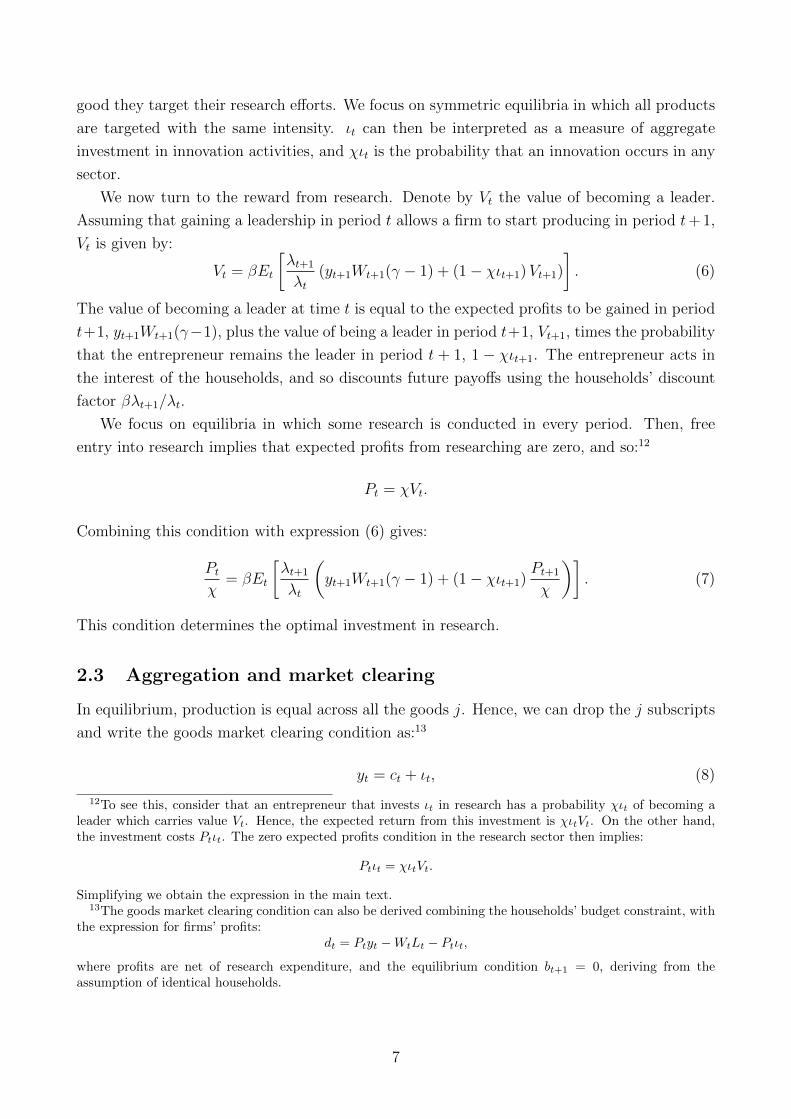
We now turn to the reward from research. Denote by Vt the value of becoming a leader.

Assuming that gaining a leadership in period t allows a firm to start producing in period t+ 1,

Vt is given by:

Vt = βEt

[λt+1

λt(yt+1Wt+1(γ − 1) + (1− χιt+1)Vt+1)

]. (6)

The value of becoming a leader at time t is equal to the expected profits to be gained in period

t+1, yt+1Wt+1(γ−1), plus the value of being a leader in period t+1, Vt+1, times the probability

that the entrepreneur remains the leader in period t + 1, 1 − χιt+1. The entrepreneur acts in

the interest of the households, and so discounts future payoffs using the households’ discount

factor βλt+1/λt.

We focus on equilibria in which some research is conducted in every period. Then, free

entry into research implies that expected profits from researching are zero, and so:12

Pt = χVt.

Combining this condition with expression (6) gives:

Ptχ

= βEt

[λt+1

λt

(yt+1Wt+1(γ − 1) + (1− χιt+1)

Pt+1

χ

)]. (7)

This condition determines the optimal investment in research.

2.3 Aggregation and market clearing

In equilibrium, production is equal across all the goods j. Hence, we can drop the j subscripts

and write the goods market clearing condition as:13

yt = ct + ιt, (8)

12To see this, consider that an entrepreneur that invests ιt in research has a probability χιt of becoming aleader which carries value Vt. Hence, the expected return from this investment is χιtVt. On the other hand,the investment costs Ptιt. The zero expected profits condition in the research sector then implies:

Ptιt = χιtVt.

Simplifying we obtain the expression in the main text.13The goods market clearing condition can also be derived combining the households’ budget constraint, with

the expression for firms’ profits:dt = Ptyt −WtLt − Ptιt,

where profits are net of research expenditure, and the equilibrium condition bt+1 = 0, deriving from theassumption of identical households.

7

which states that all the production has to be consumed or invested in research. Since labor is

the only factor of production:

yt = Lt ≤ 1, (9)

where the inequality derives from the assumption of a unitary endowment of labor. Since

labor is supplied inelastically by the households, this expression implies that when yt = 1 the

economy operates at full employment, while when yt < 1 there is involuntary unemployment.

Hence, we can interpret yt as a measure of the output gap.

Long run growth in this economy takes place through increases in the quality of the con-

sumption goods, captured by increases in the quality index Q. Since a higher Q increases the

utility that households obtain from consumption, as well as the productivity of investment in

research, we will refer to the growth rate of Q as the productivity growth rate of the economy.14

Recalling that χιt is the probability that an innovation occurs in any sector, and using the law

of large numbers, the growth rate of Q can be written as:15

gt+1 ≡Qt+1

Qt

= exp (χιt ln γ) . (10)

Hence, higher investment in research in period t is associated with faster growth between

periods t and t+ 1.

2.4 Nominal rigidities

To introduce the possibility of involuntary unemployment, and a role for monetary policy as

a stabilization tool, we consider an economy with nominal wage rigidities. For simplicity, we

start by considering an economy in which nominal wage inflation is constant and equal to π:

Wt = πWt−1. (11)

14To strengthen the parallel between the growth rate of Q and productivity growth, one could assumethat households consume a unique consumption good, produced by competitive firms using the j goods asintermediate inputs. Under this interpretation, growth in the quality of the intermediate goods would allowcompetitive firms to increase the quantity of the final good produced, and growth in the quality index Q wouldcapture the productivity growth of intermediate inputs. Grossman and Helpman (1991) show that this modelis isomorphic to the one presented in the main text.

15To derive this expression, consider that:

Qt+1 = exp

(∫[0,1]

ln qjt+1dj

)= exp

(∫It

ln γqjtdj +

∫[0,1]\It

ln qjtdj

)= exp

(∫It

ln γdj +

∫[0,1]

ln qjtdj

),

where It ∈ [0, 1] is the mass of entrepreneurs who successfully innovate at time t. The probability of successfulinnovation χιt is the same and independent across entrepreneurs, hence using the law of large numbers the lastexpression simplifies to:

exp (χιt ln γ) exp

(∫[0,1]

ln qjtdj

)= exp (χιt ln γ)Qt.

8

For instance, this expression could be derived from the presence of large menu costs from

deviating from the constant wage inflation path. Since, by equation (3), prices are proportional

to wages, it follows that also CPI inflation is constant and equal to π.

Considering an economy with constant inflation simplifies the analysis, and allows us to

characterize transparently the key economic forces at the heart of our model.16 However, in

section 3.3 we generalize our results to an economy featuring downward nominal wage rigidities,

giving rise to a Phillips curve.

2.5 Monetary policy

The central bank implements its monetary policy stance by setting the nominal interest rate

it. We consider a central bank that sets monetary policy according to the interest rate rule:

1 + it = max(

(1 + i) yφt , 1), (12)

where i > 0 and φ > 0. Under this rule, the central bank responds to a fall in the output gap,

or equivalently to a rise in unemployment, by lowering the policy rate to stimulate aggregate

demand. However, by standard arbitrage between money and bonds, the nominal interest rate

cannot be negative, it ≥ 0. Hence, there is a zero lower bound constraint on the nominal

interest rate, which might interfere with the central bank’s ability to stabilize employment.

2.6 Equilibrium

The equilibrium of our economy can be described by four simple equations. The first one

is a private aggregate demand equation, which captures households’ consumption decisions.

Combining households’ optimality conditions (1) and (2) gives the Euler equation:

C−σtQt

Pt= β(1 + it)Et

[C−σt+1Qt+1

Pt+1

].

Since households consume the same amount of every good Ct = Qtct, while constant inflation

implies Pt+1/Pt = π. Combining these two conditions with the previous expression gives the

private aggregate demand equation:

cσt =πgσ−1t+1

β(1 + it)Et[c−σt+1

] . (13)

This private aggregate demand equation relates demand for consumption with the nominal

interest rate. As it is standard in models with price rigidities, a fall in the nominal interest rate

stimulates present consumption. Similarly, a rise in expected future consumption stimulates

16In particular, focusing on an economy with constant inflation makes clear that the possibility of permanentliquidity traps in our model does not rely on self-fulfilling drops in expected inflation, of the type described byBenhabib et al. (2001).

9

present consumption.

The only non-standard feature of this aggregate demand relationship is the presence of the

growth rate of productivity, captured by the term gt+1. The impact of productivity growth on

present demand for consumption depends on the elasticity of intertemporal substitution, 1/σ.

Intuitively, there are two effects. On the one hand, faster growth generates higher lifetime

utility from consumption. This income effect leads households to increase their demand for

current consumption after a rise in the growth rate of the economy. On the other hand, faster

growth is associated with a rise in the quality of future consumption goods compared to the

quality of present consumption goods. This substitution effect points toward a negative rela-

tionship between growth and current demand for consumption. For low levels of intertemporal

substitution, i.e. for σ > 1, the income effect dominates and the relationship between growth

and demand for consumption is positive. Instead, for high levels of intertemporal substitution,

i.e. for σ < 1, the substitution effect dominates and the relationship between growth and

demand for consumption is negative. Finally, for the special case of log utility, σ = 1, the two

effects cancel out and growth does not affect present demand for consumption.

Empirical estimates based on aggregate consumption data point toward a low elasticity of

intertemporal substitution (Hall, 1988).17 Hence, in the main text we will focus attention on

the case σ > 1, while we provide an analysis of the cases σ < 1 and σ = 1 in the appendix.

Assumption 1 The parameter σ satisfies:

σ > 1.

Under this assumption, the private aggregate demand equation implies a positive relation-

ship between the pace of innovation and demand for present consumption.

The second key relationship in our model is the growth equation, which describes the sup-

ply side of the economy. To derive the growth equation, plug equations (1) and (10) in the

optimality condition for investment in research (7), and use Wt/Pt = 1/γ, to obtain:

1 = βEt

[(ctct+1

)σg1−σt+1

(χγ − 1

γyt+1 + 1− ln gt+2

ln γ

)]. (14)

This equation captures the optimal investment in research by entrepreneurs. It implies a

positive relationship between growth and the output gap, because a rise in the output gap is

associated with higher monopoly profits. In turn, higher profits induce entrepreneurs to invest

more in research, leading to a positive impact on the growth rate of the economy.

The third equation combines the goods market clearing condition (8) with the equation

17Similar results are reached by Ogaki and Reinhart (1998) and Basu and Kimball (2002). Using estimatesbased on micro data, Vissing-Jørgensen (2002) finds higher values of the elasticity of intertemporal substitution,but they still tend to be lower than 1.

10

relating growth to investment in innovation (10):

ct = yt −ln gt+1

χ ln γ. (15)

Keeping output constant, this equation implies a negative relationship between consumption

and growth, because to generate faster growth the economy has to devote a larger fraction of

the output to innovation activities, reducing the resources available for consumption.

Finally, the fourth equation is the monetary policy rule:

1 + it = max(

(1 + i) yφt , 1). (16)

We are now ready to define an equilibrium as a set of processes {yt, ct, gt+1, it}+∞t=0 satisfying

equations (13)− (16).

3 Confidence shocks and stagnation traps

In this section we show that our economy can get stuck in prolonged periods of stagnation.

We start by considering non-stochastic steady states, and show that our model features two

steady states: one characterized by full employment, and one by involuntary unemployment.

3.1 Non-stochastic steady states

In steady state growth g, the output gap y, consumption c and the nominal interest rate i are

constant. Hence, the steady state equilibrium is described by the system:

gσ−1 =β(1 + i)

π(17)

gσ−1

β+

ln g

ln γ= χ

γ − 1

γy + 1 (18)

c = y − ln g

χ ln γ(19)

1 + i = max((1 + i) yφ, 1

), (20)

where the absence of a time subscript denotes the value of a variable in a non-stochastic steady

state.

Full employment steady state. Let us start by describing the full employment steady

state, which we denote by the superscripts f . In the full employment steady state the economy

operates at full capacity (yf = 1), and so, by equation (18), productivity growth solves:(gf)σ−1β

+ln gf

ln γ= χ

γ − 1

γ+ 1. (21)

11

The nominal interest rate that supports this steady state can be obtained by rearranging

equation (17):

if =π(gf)σ−1β

− 1.

We now make some assumptions about the parameters governing the monetary policy rule,

to ensure that the full employment equilibrium exists and is unique.

Assumption 2 The parameters i, π, χ, γ, σ, β and φ satisfy:

i =π(gf)σ−1β

− 1 (22)

i ≥ 0 (23)

φ ≥ 1, (24)

where gf solves: (gf)σ−1β

+ln gf

ln γ= χ

γ − 1

γ+ 1.

Proposition 1 Suppose assumption 2 holds. Then, there exists a unique full employment

steady state.18

Intuitively, assumptions (22) and (23) guarantee that inflation and trend growth in the full

employment steady state are sufficiently high so that the zero lower bound constraint on the

nominal interest rate is not binding. In this case there exists a unique steady state in which

a positive nominal interest rate is consistent with full employment. Instead, assumption (24)

ensures that, in absence of the zero lower bound, there are no steady states other than the full

employment steady state.

Unemployment steady state. Aside from the full employment steady state, the economy

can find itself in a permanent liquidity trap with low growth and involuntary unemployment.

We denote this unemployment steady state with superscripts u. To derive the unemployment

steady state, consider that with i = 0 equation (17) implies:

gu =

(β

π

) 1σ−1

< gf ,

where the inequality holds because σ > 1. To see that the liquidity trap steady state is

characterized by unemployment, rewrite equation (18) as:

yu =

((gu)σ−1

β+

ln gu

ln γ− 1

)γ

χ(γ − 1)< 1,

where the inequality follows from gu < gf and from the fact that equation (18) gives a mono-

tonically increasing relationship between g and y. Since ι ≥ 0, this equilibrium exists if gu ≥ 1,

18All the proofs can be found in appendix A.

12

i.e. if β/π ≥ 1.19 If this is the case, assumption 2 guarantees that when the output gap is

equal to yu the central bank sets the nominal interest rate to zero. The following proposition

summarizes our results about the unemployment steady state.

Assumption 3 The parameters β and π satisfy:

β

π≥ 1.

Proposition 2 Suppose assumptions 1, 2 and 3 hold. Then, there exists a unique unemploy-

ment steady state. At the unemployment steady state the economy is in a liquidity trap (iu = 0),

there is involuntary unemployment (yu < 1), and growth is lower than in the full employment

steady state (gu < gf ).

To understand the economics behind assumption 3, consider that when i = 0, to be consis-

tent with households’ Euler equation, the economy must grow at rate (β/π)1/(σ−1). In turn, the

growth rate has a lower bound equal to 1, because knowledge does not depreciate.20 Hence,

assumption 3 guarantees that there exists a level of output gap yu > 0 consistent with the

economy growing at rate (β/π)1/(σ−1).

We think of this second steady state as a stagnation trap, that is the combination of a

liquidity and a growth trap. In a liquidity trap the economy operates below capacity because

the central bank is constrained by the zero lower bound on the nominal interest rate. In

a growth trap, lack of demand for firms’ products depresses investment in innovation and

prevents the economy from developing its full growth potential. In a stagnation trap these two

events are tightly connected. We illustrate this point with the help of a graphical analysis.

Figure 1 depicts the two key relationships that characterize the steady states of our model

in the y−g space. The first one is the growth equation (18), which corresponds to the upward-

sloped GG schedule. Intuitively, the output gap is positively related with growth because an

increase in production is associated with a rise in firms’ profits. Since firms invest in innovation

to appropriate monopoly profits, higher profits generate an increase in investment in innovation

and productivity growth, giving rise to a positive relationship between y and g.

The second key relationship combines the private aggregate demand equation (17) and the

policy rule (20):

gσ−1 =β

πmax

((1 + i)yφ, 1

).

Graphically, this relationship is captured by the AD, i.e. aggregate demand, curve. The

upward-sloped portion of the AD curve corresponds to cases in which the zero lower bound

19Since β < 1, in our baseline model an unemployment steady state exists only if inflation is non-positive,and so if π ≤ 1. However, as we show in section 3.3, this is not a strict implication of our framework, and it isnot hard to modify the model to allow for positive inflation in the unemployment steady state, for instance byintroducing precautionary savings due to idiosyncratic shocks.

20More generally, in an economy in which knowledge depreciates, an unemployment steady state exists if(β/π)1/(σ−1) is smaller than the rate of knowledge depreciation.

13

(yu, gu)

(1, gf )

AD

GG

growth

g

output gap y

Figure 1: Non-stochastic steady states.

constraint on the nominal interest rate is not binding.21 In this part of the state space, the

central bank responds to a rise in the output gap y by increasing the nominal rate. Since

inflation is constant, the increase in the nominal rate directly translates into a rise in the real

rate. In turn, according to the private aggregate demand equation, the real interest rate is

increasing in the growth rate of the economy.22 Hence, when monetary policy is active the

AD curve generates a positive relationship between y and g. Instead, the horizontal portion

of the AD curve corresponds to a situation in which the zero lower bound constraint binds. In

this case, the central bank sets i = 0 and steady state growth is independent of y and equal

to (β/π)1/(σ−1). As long as assumptions 1, 2 and 3 hold, the two curves cross twice and two

steady states are possible.

Importantly, both the presence of the zero lower bound and the procyclicality of investment

in innovation are needed to generate steady state multiplicity. Suppose that the central bank

is not constrained by the zero lower bound, and hence that liquidity traps are not possible. As

illustrated by the left panel of figure 2, in this case the AD curve reduces to an upward sloped

curve, steeper than the GG curve, and the unemployment steady state disappears. Intuitively,

in absence of the zero lower bound, the central bank’s reaction to unemployment is always

sufficiently strong to ensure that the only possible steady state is the full employment one.

Now suppose instead that productivity growth is constant and equal to gf . In this case the

GG curve reduces to a horizontal line at g = gf , and again the full employment steady state is

the only possible one. Intuitively, if growth is not affected by variations in the output gap, then

aggregate demand is always sufficiently strong so that in steady state the zero lower bound

constraint on the nominal interest rate does not bind, ensuring that the economy operates at

full employment. We refer to the unemployment steady state as a stagnation trap to capture

the tight link between liquidity and growth traps suggested by our model.

We are left with determining what makes the economy settle in one of the two steady states.

This role is fulfilled by expectations. Suppose that agents expect that the economy will per-

manently fluctuate around the full employment steady state. Then, their expectations of high

21Precisely, the zero lower bound constraint does not bind when y ≥ (1 + i)−1/φ.22Recall that we are focusing on the case σ > 1.

14

(1, gf )

AD

GG

growth

g

output gap y

(1, gf )

AD

GG

growth

g

output gap y

Figure 2: Understanding stagnation traps. Left panel: economy without zero lower bound. Right panel:economy with exogenous growth.

future growth sustain aggregate demand, so that a positive nominal interest rate is consistent

with full employment. In turn, if the economy operates at full employment then firms’ profits

are high, inducing high investment in innovation and productivity growth. Conversely, suppose

that agents expect that the economy will permanently remain in a liquidity trap. In this case,

low expectations about growth and future income depress aggregate demand, making it impos-

sible for the central bank to sustain full employment due to the zero lower bound constraint on

the interest rate. As a result the economy operates below capacity and firms’ profits are low,

so that investment in innovation is also low, justifying the initial expectations of weak growth.

Hence, in our model expectations can be self-fulfilling, and sunspots, that is confidence shocks

unrelated to fundamentals, can determine real outcomes.

Summarizing, the combination of growth driven by investment in innovation from profit-

maximizing firms and constraints on monetary policy can produce stagnation traps, that is

permanent, or very long lasting, liquidity traps characterized by unemployment and low growth.

All it takes is a sunspot that coordinates agents’ expectations on the unemployment steady

state.

3.2 Sunspots and temporary liquidity traps

Though our model can allow for economies which are permanently in a liquidity trap, it is not

difficult to construct equilibria in which the expected duration of a trap is finite.

To construct an equilibrium featuring a temporary liquidity trap we have to put some struc-

ture on the sunspot process. Let us start by denoting a sunspot by ξt. In a sunspot equilibrium

agents form their expectations about the future after observing ξ, so that the sunspot acts as

a coordination device for agents’ expectations. To be concrete, let us consider a two-state dis-

crete Markov process, ξt ∈ (ξo, ξp), with transition probabilities Pr (ξt+1 = ξo|ξt = ξo) = 1 and

Pr (ξt+1 = ξp|ξt = ξp) = qp < 1. The first state is an absorbing optimistic equilibrium, in which

agents expect to remain forever around the full employment steady state. Hence, once ξt = ξo

the economy settles on the full employment steady state, characterized by y = 1 and g = gf .

15

(yp, gp)

(1, gf )

AD

GG

growth

g

output gap y

Figure 3: Temporary liquidity trap.

The second state ξp is a pessimistic equilibrium with finite expected duration 1/(1 − qp). In

this state the economy is in a liquidity trap with unemployment. We consider an economy that

starts in the pessimistic equilibrium.

Under these assumptions, as long as the pessimistic sunspot shock persists the equilibrium

is described by equations (13), (14) and (15), which, using the fact that in the pessimistic state

i = 0, can be written as:

(gp)σ−1 =β

π

(qp + (1− qp)

(cp

cf

)σ)(25)

(gp)σ−1

β= qp

(χγ − 1

γyp + 1− ln gp

ln γ

)+ (1− qp)

(cp

cf

)σ (χγ − 1

γ+ 1− ln gf

ln γ

)(26)

cp

cf=yp − ln gp

χ ln γ

1− ln gf

χ ln γ

, (27)

where the superscripts p denote the equilibrium while pessimistic expectations prevail. Similar

to the case of the unemployment steady state, in the pessimistic equilibrium the zero lower

bound constraint on the interest rate binds, there is involuntary unemployment and growth is

lower than in the optimistic state.

While characterizing analytically the equilibrium is challenging, from equation (25) it is pos-

sible to see that temporary liquidity traps are characterized by slower growth than permanent

ones. In fact, the term cp/cf is smaller than one, because switching to the optimistic steady

state entails an increase in consumption. Intuitively, if the liquidity trap is temporary agents’

consumption is expected to rise. However, when i = 0 the real interest rate is constant and

equal to 1/π. Hence, by households’ Euler equation the expected growth rate of households’

quality-adjusted consumption is also constant, and independent of the expected duration of

the trap. It follows that, for the Euler equation to hold, the expected increase in the quantity

of goods consumed has to be compensated by a fall in the growth rate of quality. The result

is that growth is slower in a temporary liquidity trap compared to a permanent one.

Figure 3 displays the equilibrium determination in terms of the AD and GG curves. The

key change with respect to the case of non-stochastic steady states is that the AD curve is

16

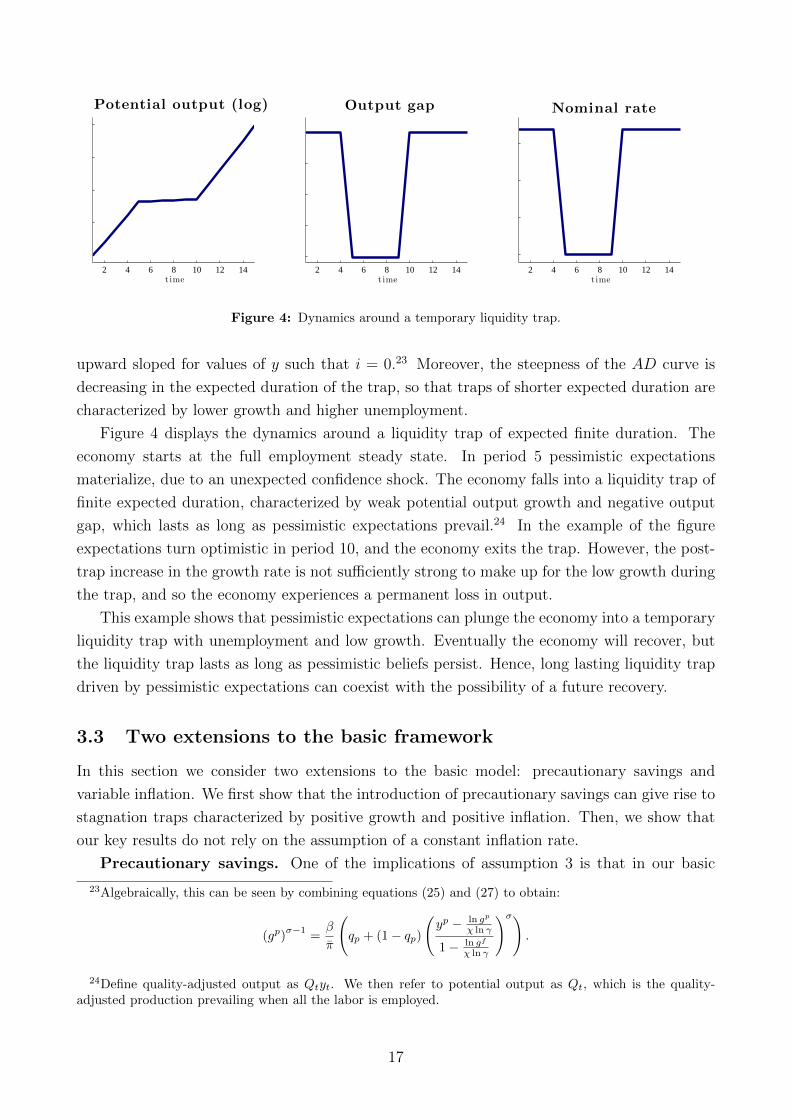
2 4 6 8 10 12 14

Potential output (log)

t ime2 4 6 8 10 12 14

Output gap

t ime2 4 6 8 10 12 14

Nominal rate

t ime

Figure 4: Dynamics around a temporary liquidity trap.

upward sloped for values of y such that i = 0.23 Moreover, the steepness of the AD curve is

decreasing in the expected duration of the trap, so that traps of shorter expected duration are

characterized by lower growth and higher unemployment.

Figure 4 displays the dynamics around a liquidity trap of expected finite duration. The

economy starts at the full employment steady state. In period 5 pessimistic expectations

materialize, due to an unexpected confidence shock. The economy falls into a liquidity trap of

finite expected duration, characterized by weak potential output growth and negative output

gap, which lasts as long as pessimistic expectations prevail.24 In the example of the figure

expectations turn optimistic in period 10, and the economy exits the trap. However, the post-

trap increase in the growth rate is not sufficiently strong to make up for the low growth during

the trap, and so the economy experiences a permanent loss in output.

This example shows that pessimistic expectations can plunge the economy into a temporary

liquidity trap with unemployment and low growth. Eventually the economy will recover, but

the liquidity trap lasts as long as pessimistic beliefs persist. Hence, long lasting liquidity trap

driven by pessimistic expectations can coexist with the possibility of a future recovery.

3.3 Two extensions to the basic framework

In this section we consider two extensions to the basic model: precautionary savings and

variable inflation. We first show that the introduction of precautionary savings can give rise to

stagnation traps characterized by positive growth and positive inflation. Then, we show that

our key results do not rely on the assumption of a constant inflation rate.

Precautionary savings. One of the implications of assumption 3 is that in our basic

23Algebraically, this can be seen by combining equations (25) and (27) to obtain:

(gp)σ−1

=β

π

(qp + (1− qp)

(yp − ln gp

χ ln γ

1− ln gf

χ ln γ

)σ).

24Define quality-adjusted output as Qtyt. We then refer to potential output as Qt, which is the quality-adjusted production prevailing when all the labor is employed.

17

framework positive growth and positive inflation cannot coexist during a permanent liquidity

trap. Intuitively, if the economy is at the zero lower bound with positive inflation, then the

real interest rate must be negative. But then, to satisfy households’ Euler equation, the steady

state growth rate of the economy must also be negative. Conversely, to be consistent with

positive steady state growth the real interest rate must be positive, and when the nominal

interest rate is equal to zero this requires deflation.

However, it is not hard to think about mechanisms that could make positive growth and

positive steady state inflation coexist in an unemployment steady state. One possibility is to

introduce precautionary savings. In appendix B, we lay down a simple model in which every

period a household faces a probability p of becoming unemployed. An unemployed household

receives an unemployment benefit, such that its income is equal to a fraction b < 1 of the

income of an employed household. Unemployment benefits are financed with taxes on the

employed households. We also assume that unemployed households cannot borrow and that

trade in firms’ share is not possible.

Under these assumptions, the private aggregate demand equation can be derived from the

Euler equation of employed households and, as showed in the appendix, can be written as:

cσt =πgσ−1t+1

β(1 + it)ρEt[c−σt+1

] ,where:

ρ ≡ 1− p+ p/bσ > 1.

The unemployment steady state is now characterized by:

gu =

(ρβ

π

) 1σ−1

.

Since ρ > 1, an unemployment steady state in which both inflation and growth are positive is

now possible.

The key intuition behind this result is that the presence of uninsurable idiosyncratic risk

depresses the natural interest rate.25 Intuitively, the presence of uninsurable idiosyncratic risk

drives up the demand for precautionary savings. Since the supply of saving instruments is fixed,

higher demand for precautionary savings leads to a lower equilibrium interest rate. This is the

reason why an economy with uninsurable unemployment risk can reconcile positive steady

state growth with a negative real interest rate. Hence, once the possibility of uninsurable

unemployment risk is taken into account, it is not hard to imagine a permanent liquidity trap

with positive growth and positive inflation.

Introducing a Phillips curve. Our basic model features a constant inflation rate. Here

we show that our results are consistent with the introduction of a Phillips curve, which creates

a positive link between inflation and the output gap.

25See Bewley (1977), Huggett (1993) and Aiyagari (1994).

18

To make things simple, let us assume that the nominal wage is downwardly rigid:

Wt ≥ ψ (yt)Wt−1,

with ψ′ > 0 and ψ(1) = π.26 This formulation, which follows Schmitt-Grohe and Uribe (2012),

allows wages to fall at a rate which depends on unemployment. Capturing some nonmonetary

costs from adjusting wages downward, here wages are more downwardly flexible the more

output is below potential. Since prices are proportional to wages, this simple form of wage

setting gives rise to a nonlinear Phillips curve. For levels of inflation greater than π output is

at potential. Instead, if inflation is below π there is a positive relationship between inflation

and the output gap.

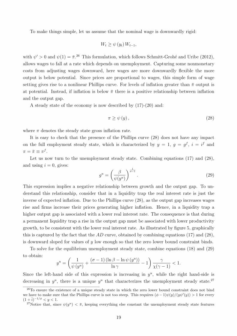
A steady state of the economy is now described by (17)-(20) and:

π ≥ ψ (y) , (28)

where π denotes the steady state gross inflation rate.

It is easy to check that the presence of the Phillips curve (28) does not have any impact

on the full employment steady state, which is characterized by y = 1, g = gf , i = if and

π = π ≡ πf .

Let us now turn to the unemployment steady state. Combining equations (17) and (28),

and using i = 0, gives:

gu =

(β

ψ(yu)

) 1σ−1

. (29)

This expression implies a negative relationship between growth and the output gap. To un-

derstand this relationship, consider that in a liquidity trap the real interest rate is just the

inverse of expected inflation. Due to the Phillips curve (28), as the output gap increases wages

rise and firms increase their prices generating higher inflation. Hence, in a liquidity trap a

higher output gap is associated with a lower real interest rate. The consequence is that during

a permanent liquidity trap a rise in the output gap must be associated with lower productivity

growth, to be consistent with the lower real interest rate. As illustrated by figure 5, graphically

this is captured by the fact that the AD curve, obtained by combining equations (17) and (28),

is downward sloped for values of y low enough so that the zero lower bound constraint binds.

To solve for the equilibrium unemployment steady state, combine equations (18) and (29)

to obtain:

yu =

(1

ψ (yu)+

(σ − 1) (ln β − lnψ (yu))

ln γ− 1

)γ

χ(γ − 1)< 1.

Since the left-hand side of this expression is increasing in yu, while the right hand-side is

decreasing in yu, there is a unique yu that characterizes the unemployment steady state.27

26To ensure the existence of a unique steady state in which the zero lower bound constraint does not bindwe have to make sure that the Phillips curve is not too steep. This requires (φ− 1)ψ(y)/(yψ′(y)) > 1 for every(1 + i)−1/φ < y < 1.

27Notice that, since ψ(yu) < π, keeping everything else constant the unemployment steady state features

19

(yu, gu)

(1, gf )

AD

GG

growth

g

output gap y

Figure 5: Steady states with variable inflation.

Moreover, since yu < 1, the presence of a Phillips curve implies that the unemployment steady

state is now characterized by lower inflation than the full employment steady state. In sum,

the presence of a Phillips curve does not alter the key properties of the unemployment steady

state, while adding the realistic feature that in the unemployment steady state the central bank

undershoots its inflation target.

4 Growth Policy

We now turn to the policy implications of our model. One of the root causes of a stagnation trap

is the weak growth performance of the economy, which is in turn due to entrepreneurs’ limited

incentives to innovate due to weak demand for their products. This suggests that subsidies

to investment in innovation or to firms’ profits might be a helpful tool in the management of

twin traps. In fact, these policies have been extensively studied in the context of endogenous

growth models as a tool to overcome inefficiencies in the innovation process. However, here we

show how policies that foster productivity growth can also play a role in stimulating aggregate

demand and employment during a liquidity trap.

The most promising form of growth policies to exit a stagnation trap are those that loosen

the link between profits and investment in innovation. For instance, suppose that the govern-

ment gives a fixed subsidy s to entrepreneurs’ investment in innovation.28 Let us also assume

that the subsidy is financed with taxes on households.29 Under these assumptions, the zero

a higher output gap and growth in the variable inflation case, compared to the model with fixed inflation.Hence, while the introduction of a Phillips curve does not alter any of our qualitative results, in quantitativeapplications it might be important to take into account the possibility that firms will respond to weak demandby cutting prices.

28More precisely, we assume that the government devotes an aggregate amount of resources s to sustaininnovation. These resources are equally divided among all the entrepreneurs operating in innovation.

29Since there is no disutility from working, it does not matter whether the subsidy is financed with lump sumtaxes on households, or with taxes on labor income.

20

profit condition in the research sector is:30

Vt =Ptχ

(1− s

ιt

).

The presence of the term s/ιt is due to the fact that entrepreneurs have to finance only a

fraction 1 − s/ιt of the investment in research, while the rest is financed by the government.

This expression implies that entrepreneurs will be willing to invest in innovation even when

the value of becoming a leader is zero, because the expression above implies that if Vt = 0 then

ιt = s. Assuming that the government can ensure that entrepreneurs cannot divert the subsidy

away from innovation activities, investment in innovation will be always at least equal to the

subsidy s, so ιt ≥ s.

Let us now consider the macroeconomic implications of the subsidy. For simplicity, we

will focus on steady states. In this case, growth in the full employment steady state is now

characterized by: ((gf)σ−1β

−(

1− ln gf

ln γ

))(1− sχ ln γ

ln gf

)= χ

γ − 1

γ, (30)

and a higher subsidy is associated with faster growth in the full employment equilibrium.31

Now turn to the unemployment steady state. In an unemployment steady state, to satisfy

the aggregate demand equation, productivity growth must be equal to gu = (β/π)(1/(σ−1)). As

discussed in section 3.1, this condition implies that an unemployment steady state exists only

if there exists a nonnegative value for the output gap such that productivity growth is equal

to gu = (β/π)(1/(σ−1)). However, a sufficiently high subsidy can guarantee that the growth

rate of the economy will always be higher than (β/π)(1/(σ−1)). It follows that by setting a

sufficiently high subsidy the government can rule out the possibility that the economy will fall

in a stagnation trap.

Proposition 3 Suppose that there is a subsidy to innovation satisfying:

s >(σ − 1) (ln β − ln π)

χ ln γ, (31)

and that the central bank sets i according to:

i =π(gf)σ−1β

− 1 ≥ 1,

30With the subsidy, the cost of investing ιt in research is Pt(ιt − s), which gives an expected gain of χιtVt.The zero expected profits condition in the research sector then implies:

Pt (ιt − s) = χιtVt.

Rearranging this expression we obtain the expression in the main text.31To ensure the existence of a full employment equilibrium, the central bank has to adjust the intercept of

the interest rate rule to take into account the impact of the subsidy on growth.

21

(yu, gu)

(1, gf )

(1, gf ′)AD

AD ′

GG

GG′

growth

g

output gap y

(yu, gu)

(1, gf )

AD

GG

GG′

growth

g

output gap y

Figure 6: Subsidy to innovation.

where gf solves equation (30), and φ ≥ 1. Then there exists a unique steady state characterized

by full employment.

Intuitively, the subsidy to innovation guarantees that even if firms’ profits were to fall

substantially, investment in innovation would still be relatively high. In turn, a high investment

in innovation stimulates growth and aggregate demand, since a high future income is associated

with a high present demand for consumption. By implementing a sufficiently high subsidy, the

government can eliminate the possibility that aggregate demand will be low enough to make the

zero lower bound constraint on the nominal interest rate bind. It is in this sense that growth

policies can be thought as a tool to manage aggregate demand in our framework. Importantly,

to be effective a subsidy to innovation has to be large enough, otherwise it might not have any

positive impact on the economy.

The left panel of figure 6 illustrates these points graphically. The solid lines correspond

to the benchmark economy, while the dashed lines represent an economy with a subsidy to

investment in innovation. The subsidy makes the GG curve shift up, because for a given level

of output gap the subsidy increases the growth rate of the economy.32 Moreover, the GG

curve has now a horizontal portion, because the subsidy places a floor in the investment in

research made by entrepreneurs. If the subsidy is sufficiently high, as it is the case in the

figure, the unemployment steady state disappears and the only possible steady state is the full

employment one.

One potential issue is that ruling out stagnation traps with a constant subsidy to innovation

could come at the cost of an inefficiently high investment in innovation in the full employment

steady state. However, it is not difficult to design a subsidy scheme that rules out the unem-

ployment steady state, while maintaining the full employment steady state unchanged. For

example, consider a countercyclical subsidy to innovation such that st = s(1− yt).Under this policy, the subsidy is decreasing in the output gap. In particular, the subsidy

is equal to zero when the economy operates at full employment, so that the full employment

steady state is not affected by the subsidy. However, if the subsidy is sufficiently large so that

32The subsidy also induces a shift left of the AD curve, because it has an impact on i.

22

condition (31) holds, this countercyclical policy rules out the unemployment steady state.

The impact of a countercyclical subsidy is illustrated by the right panel of figure 6. The

subsidy makes the GG curve rotate up. If s is sufficiently high, the movement of the curve is

large enough to eliminate the unemployment steady state, while still leaving the full employ-

ment steady state unchanged. Hence, it is possible to design subsidy schemes that rule out the

unemployment steady state without distorting the full employment one.

Summarizing, there is a role for subsidies to growth-enhancing investment, a typical sup-

ply side policy, in stimulating aggregate demand so as to rule out liquidity traps driven by

expectations of weak future growth. In turn, the stimulus to aggregate demand has a positive

impact on employment. In this sense, our model helps rationalizing the notion of job creating

growth.

5 Conclusion

We develop a Keynesian growth model in which endogenous growth interacts with the possi-

bility of involuntary unemployment due to weak aggregate demand. The model features two

steady states. One is a stagnation trap, that is a permanent liquidity trap characterized by

unemployment and weak growth. All it takes for the economy to fall into a stagnation trap is

a shift toward pessimistic expectations about future growth. Aside form permanent liquidity

traps, the model can also generate liquidity traps of arbitrarily long expected duration. We

show that large policy interventions to support growth can lead the economy out of a stagna-

tion trap, thus shedding light on the role of growth policies in stimulating aggregate demand

and employment.

Appendix

A Proofs

A.1 Proof of proposition 1 (existence and uniqueness of full em-

ployment steady state)

We start by proving existence. A steady state is described by the system:

gσ−1 =β(1 + i)

π(A.1)

gσ−1

β+

ln g

ln γ= χ

γ − 1

γy + 1 (A.2)

c = y − ln g

χ ln γ(A.3)

23

1 + i = max((1 + i) yφ, 1

), (A.4)

Setting y = 1, equation (A.2) implies:(gf)σ−1β

+ln gf

ln γ= χ

γ − 1

γ+ 1 (A.5)

Then equation (A.1) implies:

1 + if =π(gf)σ−1β

.

Assumption 2 guarantees that if ≥ 0, and that i = if , so that the interest rate rule (A.4) is

compatible with the existence of a full employment steady state. We are left to prove that

cf > 0. Combining equations (A.3) and (A.5) gives the cf > 0 if:

χ

γ+

(gf)σ−1β

> 1,

which is always the case, since gf > 1 and β < 1. Hence, the full employment steady state

exists.

To prove uniqueness, consider that equation (A.5) implies that there is only one value of g

consistent with the full employment steady state, while equation (A.1) establishes that there is

a unique value of i consistent with g = gf . Hence, the full employment steady state is unique.

�

A.2 Proof of proposition 2 (existence and uniqueness of unemploy-

ment steady state)

To prove existence, consider that when i = 0 equation (A.1) implies:

gu =

(β

π

) 1σ−1

< gf . (A.6)

Then equation (A.2) implies:

yu =

((gu)σ−1

β+

ln gu

ln γ− 1

)γ

χ(γ − 1). (A.7)

Assumption 3 guarantees that gu ≥ 1. Since 1 ≤ gu < gf , then equation (A.7) implies

0 < yu < 1, while it is easy to check that equation (A.3) implies cu > 0. To see that when

y = yu then the interest rate rule implies i = 0, suppose that this is not the case, so that:

(1 + i) (yu)φ > 1.

24

Substituting for i using equation (22), we can write the condition above as:

π

β

(gf)σ−1

(yu)φ > 1.

Combining this expression with equations (A.5), (A.6) and (A.7), and rearranging gives:

χγ−1γ

+ 1− ln gf

ln γ

χγ−1γyu + 1− ln gu

ln γ

(yu)φ > 1.

Since yu < 1 and, by assumption 2, φ > 1 the condition above cannot hold.33 Hence, we have

found a contradiction and so at the unemployment steady state the interest rate rule implies

i = 0. This proves the existence of the unemployment steady state.

To prove uniqueness, consider that when i = 0, then equation (A.6) pins down a unique

value of gu. Then equation (A.7) implies a unique value for yu, so that there exists a unique

unemployment steady state in which i = 0.

We are left to prove that it is not possible to have a steady state with unemployment if

i > 0. Suppose that this is not the case, and that there exists a steady state with i = i > 0

and y = y < 1. Then equations (A.1) and (A.2) imply:

gσ−1 =(1 + i)β

π

gσ−1

β+

ln g

ln γ= χ

γ − 1

γy + 1.

Combining the two equations above and using 1 + i = (1 + i)yφ gives:

(1 + i)

πyφ = χ

γ − 1

γy + 1− ln g

ln γ.

Substituting for i using equations (22) and (A.2) and rearranging, we can write the equation

above as:

χγ − 1

γ

(yφ − y

)+ yφ

(1− ln gf

ln γ

)−(

1− ln g

ln γ

)= 0.

Since y < 1 it follows that g < gf . Moreover, by assumption 2, φ ≥ 1. Hence, the left hand

side of this expression is negative, and we have found a contradiction. This implies that it is

not possible to have an unemployment steady state with a positive nominal interest rate. We

33To see this, consider that:

χγ − 1

γ(yu)

1−φ ≥ χγ − 1

γ,

since yu < 1 and φ ≥ 1, and that: (1− ln gu

ln γ

)(yu)

−φ>

(1− ln gf

ln γ

),

since gu < gf .

25

have thus proved uniqueness of the unemployment steady state. �

A.3 Proof of proposition 3 (steady state with subsidy to innovation)

The proof that a full employment steady state exists and is unique follows the steps of the

proof to proposition 1.

We now prove that there is no steady state with unemployment. Following the proof to

proposition 2, one can check that if another steady state exists, it must be characterized by

i = 0. Equation (A.2) implies that in this steady state growth must be equal to (β/π)(1/(σ−1)).

But with the subsidy in place, the lowest growth rate possible is exp(χs ln γ). Then, condition

(31) implies exp(χs ln γ) > (β/π)(1/(σ−1)), so that an unemployment steady state is not possible.

�

B Model with unemployment risk

In this appendix, we lay down the model with idiosyncratic unemployment risk described in

section 3.3. In this model, each household faces in every period a constant probability p of

being unemployed. The employment status is revealed to the household at the start of the

period. An unemployed household receives an unemployment benefit, such that its income

is equal to a fraction b < 1 of the income received by employed households. Unemployment

benefits are financed with taxes on employed households.

The budget constraint of a household now becomes:

ct +bt+1

1 + rt= νtWtLt + bt + dt + Tt.

The only change with respect to the benchmark model is the presence of the variables ν and

T , which summarize the impact of the employment status on a household’s budget. ν is an

indicator variable that takes value 1 if the household is employed, and 0 if the household

is unemployed. T represents a lump-sum transfer for unemployed households, and a tax for

employed households. T is set such that the income of an unemployed household is equal to a

fraction b of the income of an employed household.34

34More precisely, an unemployed household receives a transfer:

T =bWtLt + (b− 1)dt

1 + bp1−p

,

while an employed household pays a tax

T = − p

1− pbWtLt + (b− 1)dt

1 + bp1−p

.

26

Moreover, here we assume that households cannot borrow:

bt+1 ≥ 0,

and that trade in firms’ shares is not possible, so that every household receives the same

dividends d.

The Euler equation is now:

c−σt = β1 + itπ

Et[c−σt+1

]+ µt,

where µ is the Lagrange multiplier on the borrowing constraint.

We start by showing that the borrowing constraint binds only for unemployed households.

Since neither households nor firms can borrow, in equilibrium every period every household con-

sumes her entire income. Denoting, by ce and cu the consumption of respectively an employed

and an unemployed household, we have cut = bcet < cet . Moreover, due to the assumption of

i.i.d. idiosyncratic shocks, Et[c−σt+1

]is independent of the employment status. Hence, from the

Euler equation it follows that µ > 0 only for the unemployed, and so the borrowing constraint

does not bind for employed households.

The Euler equation of the employed households is:

(cet )σ =

πgσ−1t+1

β(1 + it)ρEt

[(cet+1

)−σ] ,where ρ ≡ 1 − p + p/bσ > 1, and we have used the fact that the probability of becoming

unemployed is independent of aggregate shocks. Moreover, using ct = pcut + (1 − p)cet =

cet (bp+ 1− p), we can derive the private aggregate demand equation:

cσt =πgσ−1t+1

β(1 + it)ρEt[c−σt+1

] ,which determines the demand for consumption in the model with idiosyncratic unemployment

risk.

C The cases of σ = 1 and σ < 1

In the main text we have focused attention on the empirically relevant case of low elasticity

of intertemporal substitution, by assuming that σ > 1. In this appendix we consider the

alternative cases σ = 1 and σ < 1. The key result is that, in general, under these cases the

steady state is unique.

27

We start by analyzing the case of σ = 1. In steady state, equation (17) can be written as:

1 =β(1 + i)

π.

Intuitively, under this case changes in the growth rate of the economy have no impact on the

equilibrium nominal interest rate. Hence, if there exists a full employment equilibrium featuring

a positive nominal interest rate, it is easy to check that no unemployment equilibrium can exist.

We now turn to the case σ < 1. Under this case, equation (17) implies a negative re-

lationship between growth and the nominal interest rate. Supposing that a full employment

equilibrium featuring a positive nominal interest rate exists, if a liquidity trap equilibrium ex-

ists, it must feature a higher growth rate than the full employment one, i.e. gu > gf . Since

yf = 1, it must be the case that yu ≤ yf . Now suppose that the left-hand side of equation (18)

is increasing in g. Then we cannot have a steady state in which gu > gf and yu ≤ yf , so that

an unemployment steady state cannot exist. The left-hand side of equation (18) is increasing

in g if:

g >

((1− σ) ln γ

β

) 11−σ

.

For plausible values of γ and β we have ln γ < β, implying that the inequality above always

hold and that there is a unique steady state characterized by full employment. If the inequality

above does not hold there might be multiple steady states, and the unemployment steady state

will be characterized by faster growth than the full employment one.

28

References

Aghion, Philippe, George-Marios Angeletos, Abhijit Banerjee, and Kalina Manova (2010)

“Volatility and growth: Credit constraints and the composition of investment,” Journal

of Monetary Economics, Vol. 57, No. 3, pp. 246–265.

Aghion, Philippe, Philippe Bacchetta, Romain Ranciere, and Kenneth Rogoff (2009) “Ex-

change rate volatility and productivity growth: The role of financial development,” Journal

of Monetary Economics, Vol. 56, No. 4, pp. 494–513.

Aghion, Philippe, David Hemous, and Enisse Kharroubi (2014) “Cyclical fiscal policy, credit

constraints, and industry growth,” Journal of Monetary Economics, Vol. 62, pp. 41–58.

Aghion, Philippe and Peter Howitt (1992) “A Model of Growth Through Creative Destruction,”

Econometrica, Vol. 60, No. 2, pp. 323–351.

Aiyagari, S.R. (1994) “Uninsured idiosyncratic risk and aggregate saving,” The Quarterly Jour-

nal of Economics, Vol. 109, No. 3, pp. 659–684.

Azariadis, Costas (1996) “ The Economics of Poverty Traps: Part One: Complete Markets,”

Journal of Economic Growth, Vol. 1, No. 4, pp. 449–96.

Azariadis, Costas and John Stachurski (2005) “Poverty Traps,” in Philippe Aghion and Steven

Durlauf eds. Handbook of Economic Growth, Vol. 1 of Handbook of Economic Growth: El-

sevier, Chap. 5.

Bacchetta, Philippe and Eric Van Wincoop (2013) “The great recession: a self-fulfilling global

panic,” NBER Working Paper No. 19062.

Ball, Laurence M (2014) “Long-Term Damage from the Great Recession in OECD Countries,”

NBER Working Paper No. 20185.

Barattieri, A., S. Basu, and P. Gottschalk (2010) “Some evidence on the importance of sticky

wages,” NBER Working Paper No. 16130.

Barlevy, Gadi (2004) “The Cost of Business Cycles Under Endogenous Growth,” The American

Economic Review, Vol. 94, No. 4, pp. 964–990.

Barro, Robert J and Xavier Sala-i Martin (2004) “Economic Growth,” McGraw0Hill, New

York.

Basu, Susanto and Miles Kimball (2002) “Long-run labor supply and the elasticity of intertem-

poral substitution for consumption,” manuscript, University of Michigan.

Benhabib, Jess and Roger EA Farmer (1994) “Indeterminacy and increasing returns,” Journal

of Economic Theory, Vol. 63, No. 1, pp. 19–41.

29

(1996) “Indeterminacy and sector-specific externalities,” Journal of Monetary Eco-

nomics, Vol. 37, No. 3, pp. 421–443.

Benhabib, Jess, Stephanie Schmitt-Grohe, and Martın Uribe (2001) “The perils of Taylor

rules,” Journal of Economic Theory, Vol. 96, No. 1, pp. 40–69.

Bernanke, B.S. and K. Carey (1996) “Nominal wage stickiness and aggregate supply in the

Great Depression,” The Quarterly Journal of Economics, Vol. 111, No. 3, pp. 853–883.

Bewley, T. (1977) “The Permanent Income Hypothesis and Welfare Economics,” Journal of

Economics Theory, Vol. 16, No. 2, pp. 252–292.

Cerra, V. and S.C. Saxena (2008) “Growth dynamics: the myth of economic recovery,” The

American Economic Review, Vol. 98, No. 1, pp. 439–457.

Christiano, Lawrence J, Martin S Eichenbaum, and Mathias Trabandt (2015) “Understanding

the Great Recession,” American Economic Journal: Macroeconomics, Vol. 7, No. 1, pp.

110–67.

Christiano, L.J., M. Eichenbaum, and C.L. Evans (2005) “Nominal rigidities and the dynamic

effects of a shock to monetary policy,” Journal of political Economy, Vol. 113, No. 1, pp.

1–45.

Chu, Angus C and Guido Cozzi (2014) “R&D and Economic Growth in a Cash-In-Advance

Economy,” International Economic Review, Vol. 55, No. 2, pp. 507–524.

Comin, Diego and Mark Gertler (2006) “Medium-Term Business Cycles,” The American Eco-

nomic Review, pp. 523–551.

Eggertsson, G. and P. Krugman (2012) “Debt, deleveraging, and the liquidity trap: a Fisher-

Minsky-Koo approach,” The Quarterly Journal of Economics, Vol. 127, No. 3, pp. 1469–1513.

Eggertsson, G. and M. Woodford (2003) “The zero bound on interest rates and optimal mon-

etary policy,” Brookings Papers on Economic Activity, Vol. 2003, No. 1, pp. 139–211.

Eggertsson, Gauti B (2008) “Great Expectations and the End of the Depression,” The Amer-

ican Economic Review, Vol. 98, No. 4, pp. 1476–1516.

Eggertsson, Gauti and Neil Mehrotra (2014) “A Model of Secular Stagnation,” Mimeo, Brown

University.

Eichengreen, B. and J. Sachs (1985) “Exchange Rates and Economic Recovery in the 1930s,”

The Journal of Economic History, Vol. 45, No. 4, pp. 925–946.

Fabiani, S., C. Kwapil, T. Room, K. Galuscak, and A. Lamo (2010) “Wage rigidities and labor

market adjustment in Europe,” Journal of the European Economic Association, Vol. 8, No.

2-3, pp. 497–505.

30

Farmer, Roger EA (2012) “Confidence, Crashes and Animal Spirits*,” The Economic Journal,

Vol. 122, No. 559, pp. 155–172.

Fatas, Antonio (2000) “Do business cycles cast long shadows? Short-run persistence and eco-

nomic growth,” Journal of Economic Growth, Vol. 5, No. 2, pp. 147–162.

Fehr, E. and L. Goette (2005) “Robustness and real consequences of nominal wage rigidity,”

Journal of Monetary Economics, Vol. 52, No. 4, pp. 779–804.

Francois, Patrick and Huw Lloyd-Ellis (2003) “Animal spirits through creative destruction,”

American Economic Review, pp. 530–550.

Galor, Oded and Joseph Zeira (1993) “Income Distribution and Macroeconomics,” Review of

Economic Studies, Vol. 60, No. 1, pp. 35–52.

Gottschalk, P. (2005) “Downward nominal-wage flexibility: real or measurement error?” Re-

view of Economics and Statistics, Vol. 87, No. 3, pp. 556–568.

Grossman, Gene M and Elhanan Helpman (1991) “Quality ladders in the theory of growth,”

The Review of Economic Studies, Vol. 58, No. 1, pp. 43–61.

Guerrieri, V. and G. Lorenzoni (2011) “Credit crises, precautionary savings, and the liquidity

trap,” NBER Working Paper No. 17583.

Hall, Robert E (1988) “Intertemporal Substitution in Consumption,” The Journal of Political

Economy, Vol. 96, No. 2, pp. 339–357.

Hansen, Alvin H (1939) “Economic progress and declining population growth,” The American

Economic Review, pp. 1–15.

Howitt, Peter and Philippe Aghion (1998) “Capital accumulation and innovation as com-

plementary factors in long-run growth,” Journal of Economic Growth, Vol. 3, No. 2, pp.

111–130.

Huggett, M. (1993) “The risk-free rate in heterogeneous-agent incomplete-insurance

economies,” Journal of economic Dynamics and Control, Vol. 17, No. 5-6, pp. 953–969.

Kiyotaki, Nobuhiro (1988) “Multiple expectational equilibria under monopolistic competition,”

The Quarterly Journal of Economics, pp. 695–713.

Krugman, P. (1998) “It’s baaack: Japan’s slump and the return of the liquidity trap,” Brookings

Papers on Economic Activity, Vol. 1998, No. 2, pp. 137–205.

Krugman, Paul (2013) “Secular Stagnation, Coalmines, Bubbles, and Larry Summers,” New

York Times,(Novemeber 16).

31

Matsuyama, Kiminori (1991) “Increasing Returns, Industrialization, and Indeterminacy of

Equilibrium,” The Quarterly Journal of Economics, Vol. 106, No. 2, pp. 617–50.

Murphy, Kevin M, Andrei Shleifer, and Robert W Vishny (1989) “Industrialization and the

Big Push,” Journal of Political Economy, Vol. 97, No. 5, pp. 1003–26.

Nuno, Galo (2011) “Optimal research and development and the cost of business cycles,” Journal

of Economic Growth, Vol. 16, No. 3, pp. 257–283.

Ogaki, Masao and Carmen M Reinhart (1998) “Measuring intertemporal substitution: The

role of durable goods,” Journal of Political Economy, Vol. 106, No. 5, pp. 1078–1098.

Olivei, G. and S. Tenreyro (2007) “The timing of monetary policy shocks,” The American

Economic Review, pp. 636–663.

Queralto, Albert (2013) “Financial Market Frictions, Productivity Growth and Crises in

Emerging Economies,” Mimeo, Federal Reserve Board.

Romer, Paul M (1990) “Endogenous technological change,” Journal of political Economy, pp.

S71–S102.

Schmitt-Grohe, S. and M. Uribe (2011) “Pegs and Pain,” NBER Working Paper No. 16847.

Schmitt-Grohe, Stephanie and Martın Uribe (2012) “The making of a great contraction with

a liquidity trap and a jobless recovery,” NBER Working Paper.

Summers, Lawrence (2013) “Why stagnation might prove to be the new normal,” The Financial

Times.

Vissing-Jørgensen, Annette (2002) “Limited Asset Market Participation and the Elasticity of

Intertemporal Substitution,” Journal of Political Economy, Vol. 110, No. 4.

Werning, Ivan (2011) “Managing a Liquidity Trap: Monetary and Fiscal Policy,” NBER Work-

ing Paper No. 17344.

32