Stable Manifolds of Saddle Equilibria

for Pendulum Dynamics on S2

and SO(3)

Taeyoung Lee⇤, Melvin Leok†, and N. Harris McClamroch

Abstract— Attitude control systems naturally evolve on non-

linear configurations, such as S2

and SO(3). The nontrivial

topological properties of these configurations result in interest-

ing and complicated nonlinear dynamics when studying the

corresponding closed loop attitude control systems. In this

paper, we review some global analysis and simulation techniques

that allow us to describe the global nonlinear stable manifolds

of the hyperbolic equilibria of these closed loop systems. A

deeper understanding of these invariant manifold structures are

critical to understanding the global stabilization properties of

closed loop attitude control systems, and these global analysis

techniques are applicable to a broad range of problems on

nonlinear configuration manifolds.

I. INTRODUCTION

Global nonlinear dynamics of various classes of closedloop attitude control systems have been studied in recentyears [1]. Closely related results on attitude control of aspherical pendulum (with attitude an element of the two-sphere S2) and of a 3D pendulum (with attitude an elementof the special orthogonal group SO(3)) are given in [2],[3]. These publications address the global closed dynamicsof smooth vector fields on nonlinear manifolds.

Assuming that the controlled system has an asymptoti-cally stable equilibrium, as desired in attitude stabilizationproblems, additional hyperbolic equilibria necessarily ap-pear [4]. As a result, the desired equilibrium is not globallyasymptotically stable, since the domain of attraction of thedesired asymptotically stable equilibrium excludes the unionof the stable manifolds of the hyperbolic equilibria. It isreferred to as almost globally asymptotically stable, as thestable manifolds of the hyperbolic equilibria have lowerdimension than the attitude configuration manifold. However,the characteristics of the stable manifolds to the hyperbolicequilibria and the corresponding effects on the solutions havenot been directly studied in the prior literatures.

These geometric factors motivate the current paper, inwhich new computational results to visualize the stablemanifolds of the hyperbolic equilibria are developed. Tomake the development concrete, the presentation is builtaround two specific closed loop vector fields: one for the

Taeyoung Lee, Mechanical and Aerospace Engineering, George Wash-ington University, Washington DC 20052 tlee@gwu.edu

Melvin Leok, Mathematics, University of California at San Diego, LaJolla, CA 92093 mleok@math.ucsd.edu

N. Harris McClamroch, Aerospace Engineering, University of Michigan,Ann Arbor, MI 48109 nhm@umich.edu

⇤This research has been supported in part by NSF under grants CMMI-1029551.

†This research has been supported in part by NSF under grants DMS-0726263, DMS-1001521, DMS-1010687, and CMMI-1029445.

attitude dynamics of a spherical pendulum and one for theattitude dynamics of a 3D pendulum. While the observa-tions in this paper are based on two particular examples,the computational results suggest that the existence of thehyperbolic equilibria may have nontrivial influences on thesolutions of any attitude control system, even though theirstable manifolds have zero measure. Further studies arerequired to understand the effects of the hyperbolic equilibriacompletely. Another contribution of this paper is that thepresented computational tools are also broadly applicable tostudying the geometry of more general control systems onnonlinear manifolds.

II. SPHERICAL PENDULUM

A spherical pendulum is composed of a mass m connectedto a frictionless pivot by a massless link of length l. It is actsunder uniform gravity, and it is subject to a control momentu. The configuration of a spherical pendulum is described bya unit-vector q 2 R3, representing the direction of the linkwith respect to a reference frame.

Therefore, the configuration space is the two-sphere S2 =

{q 2 R3 | q · q = 1}. The tangent space of the two-sphereat q, namely T

q

S2, is the two-dimensional plane tangent tothe unit sphere at q, and it is identified with T

q

S2 ' {! 2R3 | q · ! = 0}, using the following kinematics equation:

q = ! ⇥ q,

where the vector ! 2 R3 represents the angular velocity ofthe link. The equation of motion is given by

! =

g

lq ⇥ e3 +

1

ml2u,

where the constant g is the gravitational acceleration, andthe vector e3 = [0, 0, 1] 2 R3 denotes the unit vector alongthe direction of gravity. The control moment at the pivot isdenoted by u 2 R3.

A. Control System

Several proportional-derivative (PD) type control systemshave been developed on S2 in a coordinate-free fashion [5],[6]. Here, we summarize a control system that stabilizes aspherical pendulum to a fixed desired direction q

d

2 S2.Consider an error function on S2, representing the distance

from the direction q to the desired direction qd

, given by

(q, qd

) = 1 � q · qd

.

2011 50th IEEE Conference on Decision and Control andEuropean Control Conference (CDC-ECC)Orlando, FL, USA, December 12-15, 2011

978-1-61284-799-3/11/$26.00 ©2011 IEEE 3915

A control input is composed of a proportional term along thegradient of , and a derivative term and a cancelation term.For positive constants k

q

, k!

, it is given by

u = ml2(�kq

qd

⇥ q � k!

! � g

lq ⇥ e3).

The corresponding closed loop dynamics are written as

! = �k!

! � kq

qd

⇥ q, (1)q = ! ⇥ q. (2)

This yields two equilibrium solutions: (i) the desiredequilibrium (q, !) = (q

d

, 0); (ii) additionally, there existsanother equilibrium (�q

d

, 0) at the antipodal point.In this paper, we analyze the local stability of each

equilibrium by linearizing the closed loop dynamics to studythe equilibrium structures.

B. Linearization

Here, we develop a coordinate-free form of the linearizeddynamics of (1), (2). A variation of a curve q(t) on S2 isa family of curves q✏(t) parameterized by ✏ 2 R, satisfyingseveral properties [6]. It cannot be simply written as q✏(t) =

q(t) + ✏�q(t) for �q(t) in R3, since in general, this does notguarantee that q✏(t) lies in S2. In [7], an expression for avariation on S2 is given in terms of the exponential map asfollows:

q✏(t) = exp(✏ˆ⇠(t))q(t), (3)

for a curve ⇠(t) in R3 satisfying ⇠(t) · q(t) = 0 for all t.The hat map ˆ· : R3 ! so(3) is defined by the condition thatxy = x ⇥ y for any x, y 2 R3. The resulting infinitesimalvariation is given by

�q(t) =

d

d✏

����✏=0

q✏(t) = ⇠(t) ⇥ q(t). (4)

The variation of the angular velocity can be written as

!✏

(t) = !(t) + ✏�!(t), (5)

for a curve �w(t) in R3 satisfying q(t) · w(t) = 0 for allt. Hereafter, we do not write the dependency on time texplicitly.

Next, we substitute (4), (5) into (1), (2), and we ignorehigher-order perturbation terms. Using the fact that ⇠ · q =

! ·q = 0, and vector identities, a coordinate-free form of thelinearized equations can be written as follows:

x =

˙⇠

�!

�=

qqT ! I � qqT

kq

qd

q �kw

I

� ⇠�!

�= Ax, (6)

where the state vector of the linearized controlled systemis x = [⇠; �!] 2 R6 (see [8] for detailed derivation). Aspherical pendulum has two degrees of freedom, but thislinearized equation of motion evolves in R6 instead of R4.Since q · ! = 0 and q · ⇠ = 0, we have the following twoadditional constraints on ⇠, �!:

Cx =

qT 0

�!T q qT

� ⇠�!

�=

0

0

�. (7)

Therefore, the state vector x should lie in the null spaceof the matrix C 2 R2⇥4. However, this is not an extraconstraint that should be imposed when solving (6). As longas the initial condition x(0) satisfies (7), the structure of (1),(2), and (6), guarantees that x(t) satisfies (7) for all t, i.e.d

dt

C(t)x(t) = 0 for all t � 0 when C(0)x(0) = 0.

C. Equilibrium SolutionsWe choose the desired direction as q

d

= e3. The equi-librium solution (q

d

, 0) = (e3, 0) is referred to as thehanging equilibrium, and the additional equilibrium solution(�q

d

, 0) = (�e3, 0) is referred to as the inverted equi-librium. We study the eigen-structure of each equilibriumusing the linearized equation (6). To illustrate the ideas, thecontroller gains are selected as k

q

= k!

= 1.1) Hanging Equilibrium: The eigenvalues �

i

, and theeigenvectors v

i

of the matrix A at the hanging equilibrium(e3, 0) are given by

�1,2 = (�1 ±p

3i)/2, �3,4 = �1,2, �5 = 0, �6 = �1,

v1,2 = e1 + (�1 ±p

3i)e4/2, v3,4 = e2 + (�1 ±p

3i)e5/2,

v5 = e3, v6 = e6,

where ei

2 R6 denotes the unit-vector whose i-th elementis one, and other elements are zeros. Note that there arerepeated eigenvalues, but we obtain six linearly independenteigenvectors, i.e., the geometric multiplicities are equal tothe algebraic multiplicities.

The basis of the null space of the matrix C, namely N (C)

is {e1, e2, e4, e5}. The solution of the linearized equation canbe written as x(t) =

P6i=1 c

i

exp(�i

t)vi

for constants ci

thatare determined by the initial condition: x(0) =

P6i=1 c

i

vi

.But, the eigenvectors v5, v6 do not satisfy the constraintgiven by (7), since they do not lie in N (C). Therefore,the constants c5, c6 are zero for initial conditions that arecompatible with (7). We have Re[�

i

] < 0 for 1 i 4.Therefore, the hanging equilibrium is asymptotically stable.

2) Inverted Equilibrium: The eigenvalues �i

, and theeigenvectors v

i

of the matrix A at the inverted equilibrium(�e3, 0) are given by

�1,2 = �(

p5 + 1)/2, �3,4 = (

p5 � 1)/2, �5 = 0, �6 = �1,

v1 = e1 � (

p5 + 1)e4/2, v2 = e2 � (

p5 + 1)e5/2, (8)

v3 = (

p5 + 1)e1/2 + e4, v4 = (

p5 + 1)e2/2 + e5,

v5 = e3, v6 = e6.

The basis of N (C) is {e1, e2, e4, e5}. Hence, the eigenvec-tors v5, v6 do not lie in N (C). Therefore, the solution canbe written as x(t) =

P4i=1 c

i

exp(�i

t)vi

for constants ci

thatare determined by the initial condition.

We have Re[�1,2] < 0, and Re[�3,4] > 0. Therefore,the inverted equilibrium (q, !) = (�e3, 0) is a hyperbolicequilibrium, and in particular, a saddle equilibrium.

D. Stable Manifold for the Inverted Equilibrium1) Stable Manifold: The saddle equilibrium (�e3, 0) has

a stable manifold W s, which is defined to be

W s

(�e3, 0) = {(q, !) 2 TS2 | lim

t!1F t

(q, !) = (�e3, 0)},

3916

where F t

: (q(0), !(0)) ! (q(t), !(t)) denotes the flow mapalong the solution of (1), (2). The existence of W s

(�e3, 0)

has nontrivial effects on the overall dynamics of the con-trolled system. Trajectories in W s

(�e3, 0) converge to theantipodal point of the desired equilibrium (e3, 0), and it takesa long time period for any trajectory near W s

(�e3, 0) toasymptotically converge to the desired equilibrium (e3, 0).

According to the stable and unstable manifold theorem [9],a local stable manifold W s

loc

(�e3, 0) exists in the neighbor-hood of (�e3, 0), and it is tangent to the stable eigenspaceEs

(�e3, 0) spanned by the eigenvectors v1 and v2 of thestable eigenvalues �1,2. Then, the (global) stable manifoldcan be written as

W s

(�e3, 0) =

[

t>0

F�t

(W s

loc

(�e3, 0)), (9)

which states that the stable manifold W s can be obtained byglobalizing the local stable manifold W s

loc

by the backwardflow map.

This yields a method to compute W s

(�e3, 0) [10]. Wechoose a small ball B

�

⇢ W s

loc

(�e3, 0) with a radius �around (�e3, 0), and we grow the manifold W s

(�e3, 0) byevolving B

�

under the flow F�t. More explicitly, the stablemanifold can be parameterized by t as follows:

W s

(�e3, 0) = {F�t

(B�

)}t>0. (10)

A ball B�

in the local stable manifold can be easily chosenfrom the stable eigenspace of (�e3, 0) with a sufficientlysmall radius �. Using the stable eigenvectors v1, v2 at (8),Es

loc

(�e3, 0) can be written as

Es

loc

(�e3, 0) = {(q, !) 2 TS2 | q = exp(↵1e1 + ↵2e2)(�e3),

! = �q2(�(

p5 + 1)/2)(↵1e1 + ↵2e2) for ↵1, ↵2 2 R},

(11)

where �q2 in the expression for ! corresponds to theorthogonal projection onto the plane normal to q, as requireddue to the constraint q ·! = 0. We define a distance on TS2

as follows:

dTS2((q1, !1), (q2, !2)) =

p (q1, q2) + k!1 � !2k. (12)

Then, for a sufficiently small � > 0, B�

is expressed as(11), where the parameters ↵1, ↵2 are chosen such that thedistance from the elements on B

�

to (�e3, 0) becomes �.2) Variational Integrators: The parameterization of the

stable manifold Ws

at (10) also requires the computationof the backward flow map F�t. General purpose numericalintegrators may not preserve the structure of the two-sphereor the underlying dynamic characteristics, such as energydissipation rate, accurately, and they may yield qualitativelyincorrect numerical results in simulating a complex trajectoryover a long-time period [11].

Geometric numerical integration is concerned with devel-oping numerical integrators that preserve geometric featuresof a system, such as invariants, symmetry, and reversibility.In particular, variational integrators are geometric numericalintegrators for Lagrangian or Hamiltonian systems, con-structed according to Hamilton’s principle. They have the

e1

e2

�e3

(a) t = 8.5 (sec), k!kmax

=

0.65 (rad/s)

e1

e2

�e3

(b) t = 9 (sec), k!kmax

=

1.43 (rad/s)

e1

e2

�e3

(c) t = 8.5 (sec), k!kmax

=

2.96 (rad/s)

e1

e2

�e3

(d) t = 9 (sec), k!kmax

=

8.02 (rad/s)

Fig. 1. Stable manifold to (q,!) = (�e3

, 0) represented by{F�t

(B�)}t>0

for several values of t. One hundred points of B� inthe stable eigenspace to (�e

3

, 0) are chosen with � = 10

�6, and theyare integrated backward in time. Each trajectory is illustrated on a sphere,where the magnitude of angular velocity at each point is denoted by colorshading (red: k!k

max

, blue: k!kmin

' 0).

desirable computational properties of preserving symplec-ticity and momentum maps, and they exhibit good energybehavior [12]. A variational integrator has been developedfor Lagrangian or Hamiltonian systems evolving on the two-sphere in [7]. It preserves both the underlying symplecticproperties and the structure of the two-sphere concurrently.Here we rewrite the integrator equations in a backward form,and we use it to compute the backward flow map (see [8]for details).

3) Visualization: We choose 100 points on the surface ofB

�

with � = 10

�6, and each point is integrated backwardusing a variational integrator with a timestep of 0.002

seconds. The resulting trajectories are illustrated in Fig. 1for several values of t. Each colored curve on the sphererepresents a trajectory on TS2, since at any point q on thecurve, the direction of q is tangent to the curve at q, and themagnitude of q is indirectly represented by color shading.

We observe the following characteristics of the stablemanifold W

s

(�e3, 0) of the inverted equilibrium:

• The boundary of the stable manifold Ws

(�e3, 0) ⇢ TS2

parameterized by t is circular when projected onto S2.• Each trajectory in W

s

(�e3, 0) lies on a great circle, whenprojected onto S2. According to the closed loop dynamics(1), and the given initial condition at the surface of B

�

,the direction of ! is always parallel to !. Therefore, thedirection of ! is fixed, and the resulting trajectory of q ison a great circle. This also corresponds to the fact that the

3917

eigenvalue �1 for the first mode representing the rotationsabout the first axis is equal to the eigenvalue �2 for thesecond mode representing the rotations about the secondaxis at (8), i.e. the convergence rates of these two rotationsare identical.

• The angular velocity decreases to zero as the direction ofthe pendulum q converges to �e3.

• The stable manifold Ws

(�e3, 0) may cover S2 multipletimes if t is sufficiently large, as illustrated at Fig. 1(d).Therefore, at any point q 2 S2, we can choose ! suchthat (q, !) lies in the stable manifold W s

(�e3, 0) (thecorresponding value of ! is not unique, since if it issufficiently large, q can traverse the sphere several timesbefore converging to �e3).

The stable manifold Ws

(�e3, 0) to the inverted equilibriumhas zero measure in TS2, but as we illustrate by this example,it may cover S2 multiple times. This has strong effects onthe overall flow of the controlled system, as a trajectory hasa slower convergence rate the closer it is to W

s

(�e3, 0).

III. 3D PENDULUM

A 3D pendulum is a rigid body supported by a frictionlesspivot acting under a gravitational potential. This is a gener-alization of a planar pendulum or a spherical pendulum, asit has three rotational degrees of freedom. It has been shownthat a 3D pendulum may exhibit irregular trajectories [13].

We choose a reference frame, and a body-fixed frame.The origin of the body-fixed frame is located at the pivotpoint. The attitude of a 3D pendulum is the orientation ofthe body-fixed frame with respect to the reference frame, andit is described by a rotation matrix representing the lineartransformation from the body-fixed frame to the referenceframe. The configuration manifold is the special orthogonalgroup, SO(3) = {R 2 R3⇥3 |RTR = I, det[R] = 1}.

The equations of motion for a 3D pendulum are given by

J ˙

⌦+ ⌦⇥ J⌦ = mg⇢ ⇥ RT e3 + u,

˙R = Rˆ

⌦,

where the matrix J 2 R3⇥3 is the inertia matrix of thependulum about the pivot, and ⇢ 2 R3 is the vector fromthe pivot to the center of mass of the pendulum. The angularvelocity and the control moment at the pivot are denoted by⌦, u 2 R3, respectively. They are represented in the bodyfixed frame.

A. Control System

Several control systems have been developed onSO(3) [3], [6], [14]. Here, we summarize a control systemto stabilize a 3D pendulum to a fixed desired attitude R

d

2SO(3). Consider an attitude error function given by

(R, Rd

) =

1

2

tr⇥(I � RT

d

R)G⇤,

for a diagonal matrix G = diag[g1, g2, g3] 2 R3⇥3 withg1, g2, g3 > 0. The derivative of this attitude error function

with respect to R along the direction of �R = R⌘ for ⌘ 2 R3

is given by

DR

(R, Rd

) · �R = eR

· ⌘,

where the vee map, _ : so(3) ! R3, denotes the inverseof the hat map. An attitude error vector is defined as e

R

=

12 (GRT

d

R � RTRd

G) 2 R3. For positive constants k⌦, kR

,we choose the following control input consisting of termsproportional to the attitude error vector and the angularvelocity vector and a cancellation term:

u = �kR

eR

� k⌦⌦� mg⇢ ⇥ RT e3.

The corresponding closed loop dynamics are given by

J ˙

⌦ = �⌦⇥ J⌦� kR

eR

� k⌦⌦, (13)˙R = Rˆ

⌦. (14)

This system has four equilibria: in addition to the desiredequilibrium (R

d

, 0), there exist three other equilibria at(R

d

exp(⇡ei

, 0), 0) for i 2 {1, 2, 3}, which correspond tothe rotation of the desired attitude by 180

� about each body-fixed axis. The existence of additional, undesirable equilibriais due to the nontrivial topological structure of SO(3), and itcannot be avoided by constructing a different control system(as long as it is continuous). It has been shown that it is notpossible to design a continuous feedback control stabilizingan attitude globally on SO(3) [4], [15].

In this paper, we linearize the closed loop dynamics tostudy the stability of each equilibrium.

B. LinearizationA variation in SO(3) can be expressed as:

R✏

= R exp(✏⌘), ⌦

✏

= ⌦+ ✏�⌦, (15)

for ⌘, �⌦ 2 R3. The corresponding infinitesimal variation ofR is given by �R = R⌘. Substituting these into (13), (14),we obtain the linearized equation as follows:

x =

⌘

� ˙

⌦

�=

"�ˆ

⌦ I

� 12k

R

J�1H J�1(

cJ⌦� ˆ

⌦J � k⌦I)

# ⌘

�⌦

�

= Ax, (16)

where H = tr[RTRd

G]I � RTRd

G 2 R3⇥3 (see [8] fordetails).

C. Equilibrium SolutionsWe choose the desired attitude as R

d

= I . In addition tothe desired equilibrium (I, 0), there are three additional equi-libria, namely (exp(⇡e1), 0), (exp(⇡e2), 0), (exp(⇡e3), 0).We assume that

J = diag[3, 2, 1] kgm

2, G = diag[0.9, 1, 1.1], kR

= k⌦ = 1.

1) Equilibrium (I, 0): The eigenvalues of the matrix A atthe desired equilibrium (I, 0) are given by

�1,2 = �0.1667 ± 0.5676i,

�3,4 = �0.25 ± 0.6614i,

�5,6 = �0.5 ± 0.8367i.

This equilibrium is an asymptotically stable focus.

3918

2) Equilibrium (exp(⇡e1), 0): At this equilibrium, theeigenvalues and the eigenvectors of A are given by

�1 = �0.7813, v1 = e1 + �1e4,

�2 = �0.5854, v2 = e2 + �2e5,

�3 = �1.0477, v3 = e3 + �3e6, (17)�4 = 0.4480, v4 = e1 + �4e4,

�5 = 0.0854, v5 = e2 + �5e5,

�6 = 0.0477, v6 = e3 + �6e6.

Therefore, this equilibrium is a saddle equilibrium, wherethree modes are stable, and three modes are unstable.

3) Equilibrium (exp(⇡e2), 0): At this equilibrium, theeigenvalues and the eigenvectors of A are given by

�1 = �0.3775, v1 = e1 + �1e4,

�2 = �1, v2 = e2 + �2e5, (18)�3 = �0.9472, v3 = e3 + �3e6,

�4 = �0.0528, v4 = e3 + �4e6,

�5 = 0.0442, v5 = e1 + �5e4,

�6 = 0.5, v6 = e2 + �6e5.

Therefore, this equilibrium is a saddle equilibrium, wherefour modes are stable, and two modes are unstable.

4) Equilibrium (exp(⇡e3), 0): At this equilibrium, theeigenvalues and the eigenvectors of A are given by

�1 = �0.0613, v1 = e1 + �1e4,

�2 = �0.2721, v2 = e1 + �2e4,

�3 = �0.1382, v3 = e2 + �3e5,

�4 = �0.3618, v4 = e2 + �4e5,

�5 = �1.5954, v5 = e3 + �5e6, (19)�6 = 0.5954, v6 = e2 + �6e6.

Therefore, this equilibrium is a saddle equilibrium, wherefive modes are stable, and one mode is unstable.

D. Stable Manifolds for the Saddle Equilibria

Eigen-structure analysis shows that there exist multi-dimensional stable manifolds for each saddle equilibrium.They have zero measure as the dimension of the stablemanifold is less than the dimension of TSO(3). But, theexistence of these stable manifolds may have nontrivialeffects on the attitude dynamics. We numerically characterizethese stable manifolds using backward time integration, asdiscussed in Section II-D.

The stable eigenspace for each saddle equilibrium can bewritten in terms of eigenvectors similar to (11). For example,the stable eigenspace for (exp(⇡e3), 0) is given by

Es

loc

(exp(⇡e3), 0) = {(R,⌦) 2 TSO(3) |R = exp(⇡e3) exp((↵1 + ↵2)e1 + (↵3 + ↵4)e2 + ↵5e3),

⌦ = (�1↵1 + �2↵2)e1 + (�3↵3 + �4↵4)e2

� �5↵5e3 for ↵i

2 R},

e2e1

e3

(a) Visualization on sphere

0 0.2 0.4 0.6 0.8 1ï30

ï20

ï10

0

�

0 0.2 0.4 0.6 0.8 10

0.5

1

t

˙ �

(b) Rotation angle � (deg), and rota-tion rate ˙� (rad/sec)

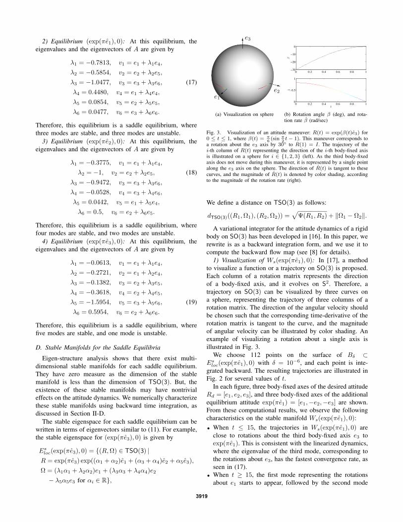
Fig. 3. Visualization of an attitude maneuver: R(t) = exp(�(t)e3

) for0 t 1, where �(t) =

⇡6

(sin

⇡2

t � 1). This maneuver corresponds toa rotation about the e

3

axis by 30

� to R(1) = I . The trajectory of thei-th column of R(t) representing the direction of the i-th body-fixed axisis illustrated on a sphere for i 2 {1, 2, 3} (left). As the third body-fixedaxis does not move during this maneuver, it is represented by a single pointalong the e

3

axis on the sphere. The direction of ˙R(t) is tangent to thesecurves, and the magnitude of ˙R(t) is denoted by color shading, accordingto the magnitude of the rotation rate (right).

We define a distance on TSO(3) as follows:

dTSO(3)((R1,⌦1), (R2,⌦2)) =

p (R1, R2) + k⌦1 � ⌦2k.

A variational integrator for the attitude dynamics of a rigidbody on SO(3) has been developed in [16]. In this paper, werewrite is as a backward integration form, and we use it tocompute the backward flow map (see [8] for details).

1) Visualization of Ws

(exp(⇡e1), 0): In [17], a methodto visualize a function or a trajectory on SO(3) is proposed.Each column of a rotation matrix represents the directionof a body-fixed axis, and it evolves on S2. Therefore, atrajectory on SO(3) can be visualized by three curves ona sphere, representing the trajectory of three columns of arotation matrix. The direction of the angular velocity shouldbe chosen such that the corresponding time-derivative of therotation matrix is tangent to the curve, and the magnitudeof angular velocity can be illustrated by color shading. Anexample of visualizing a rotation about a single axis isillustrated in Fig. 3.

We choose 112 points on the surface of B�

⇢Es

loc

(exp(⇡e1), 0) with � = 10

�6, and each point is inte-grated backward. The resulting trajectories are illustrated inFig. 2 for several values of t.

In each figure, three body-fixed axes of the desired attitudeR

d

= [e1, e2, e3], and three body-fixed axes of the additionalequilibrium attitude exp(⇡e1) = [e1,�e2,�e3] are shown.From these computational results, we observe the followingcharacteristics on the stable manifold W

s

(exp(⇡e1), 0):• When t 15, the trajectories in W

s

(exp(⇡e1), 0) areclose to rotations about the third body-fixed axis e3 toexp(⇡e1). This is consistent with the linearized dynamics,where the eigenvalue of the third mode, corresponding tothe rotations about e3, has the fastest convergence rate, asseen in (17).

• When t � 15, the first mode representing the rotationsabout e1 starts to appear, followed by the second mode

3919

e2

e1

e3

�e2

�e3

(a) t = 11 (sec), k⌦kmax

=

0.06 (rad/s)

e2

e1

e3

�e2

�e3

(b) t = 12 (sec), k⌦kmax

=

0.17 (rad/s)

e2

e1

e3

�e2

�e3

(c) t = 13 (sec), k⌦kmax

=

0.50 (rad/s)

e2

e1

e3

�e2

�e3

(d) t = 14 (sec), k⌦kmax

=

1.42 (rad/s)

e2

e1

e3

�e2

�e3

(e) t = 15 (sec), k⌦kmax

=

3.93 (rad/s)

e2

e1

e3

�e2

�e3

(f) t = 16 (sec), k⌦kmax

=

10.67 (rad/s)

e2

e1

e3

�e2

�e3

(g) t = 17 (sec), k⌦kmax

=

29.00 (rad/s)

e2

e1

e3

�e2

�e3

(h) t = 18 (sec), k⌦kmax

=

78.84 (rad/s)

Fig. 2. Stable manifold to (exp(⇡e1

), 0) = ([e1

,�e2

,�e3

], 0) represented by {F�t(B�)}t>0

with � = 10

�6 for several values of t.

representing the rotation about e2. This corresponds to thefact that the first mode has a faster convergence rate thanthe second mode, i.e. |�1| > |�2|.

• As t is increased further, the third body-fixed axis leavesthe neighborhood of �e3, and it exhibit the followingpattern:

• The stable manifold Ws

(exp(⇡e1), 0) covers a certain partof SO(3), when projected on to it. So, when an initialattitude is chosen such that its third body-fixed axis issufficiently close to �e3, there possibly exist multiple ini-tial angular velocities such that the corresponding solutionconverges to exp(⇡e1) instead of the desired attitude, I .

2) Visualization of Ws

(exp(⇡e2), 0): Similarly, we com-pute W

s

(exp(⇡e2), 0) from 544 points. The resulting tra-jectories are illustrated in Fig. 4 for several values of t.From these computational results, we observe the followingcharacteristics on the stable manifold W

s

(exp(⇡e2), 0):

• When t 12, the trajectories in Ws

(exp(⇡e2), 0) isclose to the rotations about the second body-fixed axise2. As t increases, rotations about e3 starts to appear.This corresponds to the linearized dynamics where thesecond mode representing rotations about e2 has the fastestconvergence rate, followed by the third mode at (18).

• As t is increased further, nonlinear modes become dom-

inant. The trajectories in Ws

(exp(⇡e2), 0) almost coverSO(3). This suggests that for any initial attitude, wecan choose several initial angular velocities such that thecorresponding solutions converges to exp(⇡e2).3) Visualization of W

s

(exp(⇡e3), 0): We also computeW

s

(exp(⇡e3), 0) from 976 points. The resulting trajectoriesare illustrated in Fig. 5 for several values of t. From thesecomputational results, we observe the following characteris-tics on the stable manifold W

s

(exp(⇡e3), 0):• When t 8, the trajectories in W

s

(exp(⇡e3), 0) areclose to the rotations about the third body-fixed axis e3.This corresponds to the linearized dynamics where thefifth mode representing rotations about e3 has the fastestconvergence rate given in (19).

• The rotations about e3 are still dominant, even as tis increased further. For the given simulation times, alltrajectories are close to rotations about e3.In a 3D Pendulum, the characteristics of stable manifolds

can vary widely depending on the equilibria. We observe thatW

s

(exp(⇡e3), 0) has a higher dimension, but it has simplertrajectories over the time period considered in this paper.The trajectories in W

s

(exp(⇡e2), 0) are most complicated,and they cover a large part of SO(3). This illustrates thatthe existence of stable manifolds of the saddle equilibria hasimportant effects to the global dynamics of the controlledsystem.

REFERENCES

[1] N. A. Chaturvedi, A. K. Sanyal, and N. H. McClamroch, “Rigid bodyattitude control: Using rotation matrices for continuous, singularity-free control laws,” IEEE Control Systems Magazine, pp. 30–51, 2011.

3920

e1

e2

e3

�e1

�e3

(a) t = 11 (sec), k⌦kmax

=

0.03 (rad/s)

e1

e2

e3

�e1

�e3

(b) t = 12 (sec), k⌦kmax

=

0.09 (rad/s)

e1

e2

e3

�e1

�e3

(c) t = 13 (sec), k⌦kmax

=

0.25 (rad/s)

e1

e2

e3

�e1

�e3

(d) t = 14 (sec), k⌦kmax

=

0.69 (rad/s)

e1

e2

e3

�e1

�e3

(e) t = 15 (sec), k⌦kmax

=

1.69 (rad/s)

e1

e2

e3

�e1

�e3

(f) t = 16 (sec), k⌦kmax

=

3.37 (rad/s)

e1

e2

e3

�e1

�e3

(g) t = 17 (sec), k⌦kmax

=

7.01 (rad/s)

e1

e2

e3

�e1

�e3

(h) t = 18 (sec), k⌦kmax

=

18.22 (rad/s)

Fig. 4. Stable manifold to (exp(⇡e2

), 0) = ([�e1

, e2

,�e3

], 0) represented by {F�t(B�)}t>0

with � = 10

�6 for several values of t.

�e1

e2

e3

e1

�e2

(a) t = 8 (sec), k⌦kmax

=

0.224 (rad/s)

�e1

e2

e3

e1

�e2

(b) t = 9 (sec), k⌦kmax

=

1.09 (rad/s)

�e1

e2

e3

e1

�e2

(c) t = 10 (sec), k⌦kmax

=

4.26 (rad/s)

�e1

e2

e3

e1

�e2

(d) t = 14 (sec), k⌦kmax

=

222.99 (rad/s)

Fig. 5. Stable manifold to (exp(⇡e3

), 0) = ([�e1

,�e2

, e3

], 0) represented by {F�t(B�)}t>0

with � = 10

�6 for several values of t.

[2] N. A. Chaturvedi, N. H. McClamroch, and D. S. Bernstein, “Stabi-lization of a 3D axially symmetric pendulum,” Automatica, pp. 2258–2265, 2008.

[3] N. Chaturvedi, N. H. McClamroch, and D. Bernstein, “Asymptoticsmooth stabilization of the inverted 3-D pendulum,” IEEE Transac-tions on Automatic Control, vol. 54, no. 6, pp. 1204–1215, 2009.

[4] D. Koditschek, “Application of a new lyapunov function to globaladaptive tracking,” in Proceedings of the IEEE Conference on Decisionand Control, 1998, pp. 63–68.

[5] F. Bullo, R. M. Murray, and A. Sarti, “Control on the sphere andreduced attitude stabilization,” in IFAC Symposium on NonlinearControl Systems, vol. 2, 1995, pp. 495–501.

[6] F. Bullo and A. Lewis, Geometric control of mechanical systems.Springer, 2005.

[7] T. Lee, M. Leok, and N. H. McClamroch, “Lagrangian mechanicsand variational integrators on two-spheres,” International Journal forNumerical Methods in Engineering, vol. 79, pp. 1147–1174, 2009.

[8] T. Lee, M. Leok, and N. McClamroch, “Stable manifolds of saddlepoints for pendulum dynamics on S2 and SO(3),” arXiv:1103.2822v1.[Online]. Available: http://arxiv.org/abs/1103.2822v1

[9] Y. Kuznetsov, Elements of Applied Bifurcation Theory. Springer,1998.

[10] B. Krauskopf, H. Osinga, E. Doedel, M. Henderson, J. Guckenheimer,

A. Vladimirsky, M. Dellnitz, and O. Junge, “A survey of methods forcomputing (un)stable manifolds of vector fields a survey of methodsfor computing (un)stable manifolds of vector fields,” InternationalJournal of Bifurcation and Chaos, vol. 15, no. 3, pp. 763–791, 2005.

[11] E. Hairer, C. Lubich, and G. Wanner, Geometric numerical integration,ser. Springer Series in Computational Mechanics 31. Springer, 2000.

[12] J. Marsden and M. West, “Discrete mechanics and variational integra-tors,” in Acta Numerica. Cambridge, 2001, vol. 10, pp. 317–514.

[13] N. Chaturvedi, T. Lee, M. Leok, and N. H. McClamroch, “Nonlineardynamics of the 3D pendulum,” Journal of Nonlinear Science, vol. 21,no. 1, pp. 3–21, 2011.

[14] T. Lee, “Geometric tracking control of the attitude dynamics of a rigidbody on SO(3),” in Proceeding of the American Control Conference,2011, pp. 1885–1891.

[15] S. Bhat and D. Bernstein, “A topological obstruction to continuousglobal stabilization of rotational motion and the unwinding phe-nomenon,” Systems and Control Letters, vol. 39, pp. 66–73, 2000.

[16] T. Lee, M. Leok, and N. H. McClamroch, “Lie group variationalintegrators for the full body problem in orbital mechanics,” CelestialMechanics and Dynamical Astronomy, vol. 98, pp. 121–144, 2007.

[17] ——, “Global symplectic uncertainty propagation on SO(3),” in Pro-ceedings of the IEEE Conference on Decision and Control, 2008, pp.61–66.

3921