
Stabilization, Extension and Unification of the Lattice ... Extension and Uni cation of the Lattice...
98
Stabilization, Extension and Unification of the Lattice Boltzmann Method Using Information Theory by Tyler Wilson A thesis submitted in conformity with the requirements for the degree of Doctor of Philosophy Graduate Department of Mathematics University of Toronto c Copyright 2016 by Tyler Wilson
Transcript of Stabilization, Extension and Unification of the Lattice ... Extension and Uni cation of the Lattice...

Stabilization, Extension and Unification of the Lattice BoltzmannMethod Using Information Theory
by
Tyler Wilson
A thesis submitted in conformity with the requirementsfor the degree of Doctor of PhilosophyGraduate Department of Mathematics
University of Toronto
c© Copyright 2016 by Tyler Wilson

Abstract
Stabilization, Extension and Unification of the Lattice Boltzmann Method Using Information
Theory
Tyler Wilson
Doctor of Philosophy
Graduate Department of Mathematics
University of Toronto
2016
A novel Lattice Boltzmann method is derived using the Principle of Minimum Discrimination Infor-
mation (MinxEnt) via the minimization of Kullback-Leibler Divergence (KLD). Approximations of
this method yield the single relaxation time (SRT-LBM), two relaxation time (TRT-LBM), multiple
relaxation time (MRT-LBM) Lattice Boltzmann Methods as well as Entropic Lattice Boltzmann
Method (ELBM) and Ehrenfest Step LBM (EF-LBM). Specifically it is shown that these methods
can be understood as approximations of a method for constrained KLD minimization. By carry-
ing out the actual single step Newton-Raphson minimization (MinxEnt-LBM) a more accurate and
stable Lattice Boltzmann Method can be implemented. To demonstrate this, 2D Poiseulle flow,
1D shock tube and lid-driven cavity flow simulations are carried out and compared to SRT-LBM,
TRT-LBM MRT-LBM and EF-LBM.
ii

To my Mom and Dad.
You did this. I just put my name on it.
iii

Acknowledgements
Firstly, I would like to express my sincerest gratitude to my advisors Prof. Mary Pugh and Prof.
Francis Dawson for their continuous support of my work and most of all for their seemingly endless
patience. Their guidance helped me in both the research and writing phases of this thesis. I could
not have imagined having better advisors and mentors for my Ph.D study. I, and my family, cannot
thank you both enough.
I would like to thank the third member of my thesis committee: Prof. Almut Burchard, for her
insightful comments and encouragement, particularly when things looked most bleak. In addition,
I would like to thank Prof. Clinton Groth and Prof. Robert McCann. Both have been extremely
generous with their time, not only in agreeing to serve on my defense committee, but for all the
helpful conversations along the wandering path of this work. To Prof. Adrian Nachman, thank
you for agreeing to serve on my defense committee. In a real and practical sense, this wouldn’t be
possible without your kind help.
Throughout the many twists and turns of my research I reached out to a number of experts in
the field including Prof. Li-Shi Luo, Prof. Michael Sukop and Prof. Tony Ladd. A heartfelt thanks
to each of you for taking the time out of your busy lives to offer honest, interesting and thoughtful
feedback to an unknown student from thousands of kilometers away.
As any student can attest, a single word of this thesis could not have been written if not for the
financial support of many people along the way. Chief among them I would like to thank Angella
Hughes and the Board of Directors of Xogen Technologies for the considerable investment in my
work and my future. Not only from the financial side of things but also for providing me a long list
of professional and personal growth experiences that have already proven to be invaluable. Also,
thank you to the University of Toronto for allowing me the opportunity to assist and teach a number
of classes throughout the years. Teaching has truly been one of the most rewarding experiences of
my young career and something that will certainly be part of my future. Finally, this work was
also generously supported by the Natural Sciences and Engineering Research Council of Canada and
MITACS. Therefore, thank you to the people at NSERC, MITACS and also to the taxpayers of
Canada, most of whom have not been given the opportunities I have and yet selflessly contributed
to this work.
Thank you to all of my friends, colleagues, students and teammates who provided so many
interesting and enjoyable times during my stay at the University of Toronto. You served as just
enough to distraction to keep me sane, but not quite enough to prevent this work from being
completed.
Last and certainly not least, thank you to my family. To my beautiful (and inhumanly patient)
wife I couldn’t have accomplished any of this without your unwavering support. Along the way you
fostered this work, but also set the highest standard for my ongoing effort to be a better citizen of
society. Your energy, kindness and compassion are truly endless. Lastly, thank you to my daughter
whose hugs and laughter makes all of this, and everything else, worth it.
iv

Contents
1 Introduction 1
2 Lattice Boltzmann Methods 7
2.1 LBM Simulation Procedure . . . . . . . . . . . . . . . . . . . . . . . . . . . . . . . . 7
2.1.1 Equilibrium Distributions . . . . . . . . . . . . . . . . . . . . . . . . . . . . . 9
2.1.2 Collision Step: Single Relaxation Time (SRT-LBM) . . . . . . . . . . . . . . 10
2.1.3 Collision Step: Multiple Relaxation Time (MRT-LBM) . . . . . . . . . . . . 11
2.1.4 Collision Step: Entropic Lattice Boltzmann Method (ELBM) . . . . . . . . . 12
2.1.5 Collision Step: SRT-LBM with Ehrenfest Steps (EF-LBM) . . . . . . . . . . 12
2.1.6 Discretization: D2Q9 Scheme Example . . . . . . . . . . . . . . . . . . . . . . 13
2.1.7 Boundary Conditions . . . . . . . . . . . . . . . . . . . . . . . . . . . . . . . 16
3 Principle of Minimum Discrimination Information (MinxEnt) 18
4 MinxEnt Lattice Boltzmann Method (MinxEnt-LBM) 22
4.1 The MinxEnt-LBM Collision Step . . . . . . . . . . . . . . . . . . . . . . . . . . . . 22
4.1.1 Discretization Scheme . . . . . . . . . . . . . . . . . . . . . . . . . . . . . . . 23
4.1.2 Minimization Method: Newton-Raphson . . . . . . . . . . . . . . . . . . . . . 24
4.1.3 Minimization Method: “Iterative Interpolation” . . . . . . . . . . . . . . . . . 26
4.2 Unification of LBM Methods . . . . . . . . . . . . . . . . . . . . . . . . . . . . . . . 28
4.2.1 MRT-LBM as an Approximation of MinxEnt-LBM . . . . . . . . . . . . . . 29
4.2.2 SRT-LBM With Ehrenfest Steps as an Approximation of MinxEnt-LBM . . . 31
4.2.3 ELBM as an Implementation of MinxEnt-LBM . . . . . . . . . . . . . . . . . 32
4.2.4 Conclusion . . . . . . . . . . . . . . . . . . . . . . . . . . . . . . . . . . . . . 33
4.3 MinxEnt-LBM For Athermal 2-D Isotropic Newtonian Fluids . . . . . . . . . . . . . 34
4.3.1 Choice of q(v) . . . . . . . . . . . . . . . . . . . . . . . . . . . . . . . . . . . 34
4.3.2 Choice of Constraints . . . . . . . . . . . . . . . . . . . . . . . . . . . . . . . 34
4.3.3 Discretization in D2Q9 . . . . . . . . . . . . . . . . . . . . . . . . . . . . . . . 35
4.3.4 Choice of Minimization Procedure; MinxEnt-LBM Using Newton-Raphson in
Moment Space . . . . . . . . . . . . . . . . . . . . . . . . . . . . . . . . . . . 37
5 Numerical Applications 41
5.1 General Considerations . . . . . . . . . . . . . . . . . . . . . . . . . . . . . . . . . . . 41
5.1.1 Velocity Discretization . . . . . . . . . . . . . . . . . . . . . . . . . . . . . . . 41
5.1.2 Collision Steps . . . . . . . . . . . . . . . . . . . . . . . . . . . . . . . . . . . 42
5.1.3 Boundary Conditions and Initial Conditions . . . . . . . . . . . . . . . . . . . 43
5.2 2D Poiseulle Flow Convergence Studies . . . . . . . . . . . . . . . . . . . . . . . . . . 44
5.2.1 Results . . . . . . . . . . . . . . . . . . . . . . . . . . . . . . . . . . . . . . . 44
v

5.3 1D Shock tube . . . . . . . . . . . . . . . . . . . . . . . . . . . . . . . . . . . . . . . 44
5.3.1 Results . . . . . . . . . . . . . . . . . . . . . . . . . . . . . . . . . . . . . . . 46
5.4 Lid-Driven Cavity Flow: Stability Studies . . . . . . . . . . . . . . . . . . . . . . . . 46
5.4.1 Results . . . . . . . . . . . . . . . . . . . . . . . . . . . . . . . . . . . . . . . 48
5.5 Lid-Driven Cavity Flow: Accuracy Studies . . . . . . . . . . . . . . . . . . . . . . . . 48
5.5.1 Results . . . . . . . . . . . . . . . . . . . . . . . . . . . . . . . . . . . . . . . 49
5.6 Discussion . . . . . . . . . . . . . . . . . . . . . . . . . . . . . . . . . . . . . . . . . . 58
6 Conclusions 70
6.1 Conclusions . . . . . . . . . . . . . . . . . . . . . . . . . . . . . . . . . . . . . . . . . 70
6.2 Future Work . . . . . . . . . . . . . . . . . . . . . . . . . . . . . . . . . . . . . . . . 71
Appendices 72
A Probability and Mass Expectation Distributions 73
B D2Q9 Fluid Constraint 77
B.1 Isotropic Newtonain Fluids . . . . . . . . . . . . . . . . . . . . . . . . . . . . . . . . 77
B.2 D2Q9 LBM Configuration . . . . . . . . . . . . . . . . . . . . . . . . . . . . . . . . . 77
B.3 D2Q9 Tensor Identities . . . . . . . . . . . . . . . . . . . . . . . . . . . . . . . . . . . 78
B.4 Chapman-Enskog Expansion . . . . . . . . . . . . . . . . . . . . . . . . . . . . . . . 78
B.5 Consequences of Equilibrium and Collision Constraints . . . . . . . . . . . . . . . . . 79
B.6 Discussion . . . . . . . . . . . . . . . . . . . . . . . . . . . . . . . . . . . . . . . . . . 82
vi

List of Tables
2.1 D2Q9 Velocity Scheme: c =√
3RT . . . . . . . . . . . . . . . . . . . . . . . . . . . . 14
5.1 The D2Q9 velocity scheme in lattice units and RT = 1 . . . . . . . . . . . . . . . . . 42
5.2 Relaxation times for the various LBM collisions. The values 1.64 and 1.54 are chosen
to agree with [53, 43]. Tolerance values are given in (5.3). ∆S is defined in (2.9) . . 43
5.3 Simulation setup for 2D Poiseulle flow convergence tests . . . . . . . . . . . . . . . . 45
5.4 Simulation setup for 1D shock tube . . . . . . . . . . . . . . . . . . . . . . . . . . . . 46
5.5 Simulation setup for lid-driven flow stability tests . . . . . . . . . . . . . . . . . . . . 47
5.6 Simulation setup for lid-driven flow . . . . . . . . . . . . . . . . . . . . . . . . . . . . 51
5.7 Run Times For Lid Driven Accuracy Studies (time in seconds) . . . . . . . . . . . . 55
5.8 Run Times For Lid Driven Accuracy Studies (time in seconds) . . . . . . . . . . . . 56
5.9 Run Times For Lid Driven Accuracy Studies (time in seconds) . . . . . . . . . . . . 57
5.10 Main Vortex Results, Nx =65 . . . . . . . . . . . . . . . . . . . . . . . . . . . . . . . 59
5.11 Main Vortex Results, Nx =129 . . . . . . . . . . . . . . . . . . . . . . . . . . . . . . 64
5.12 Main Vortex Results, Nx =257 . . . . . . . . . . . . . . . . . . . . . . . . . . . . . . 65
5.13 Lower Right Vortex Results, Nx =65 . . . . . . . . . . . . . . . . . . . . . . . . . . . 65
5.14 Lower Right Vortex Results, Nx =129 . . . . . . . . . . . . . . . . . . . . . . . . . . 66
5.15 Lower Right Vortex Results, Nx =257 . . . . . . . . . . . . . . . . . . . . . . . . . . 67
5.16 Lower Left Vortex Results, Nx=65 . . . . . . . . . . . . . . . . . . . . . . . . . . . . 67
5.17 Lower Left Vortex Results, Nx =129 . . . . . . . . . . . . . . . . . . . . . . . . . . . 68
5.18 Lower Left Vortex Results, Nx =257 . . . . . . . . . . . . . . . . . . . . . . . . . . . 69
B.1 D2Q9 Velocity Scheme: c =√
3RT . . . . . . . . . . . . . . . . . . . . . . . . . . . . 77
vii
List of Figures
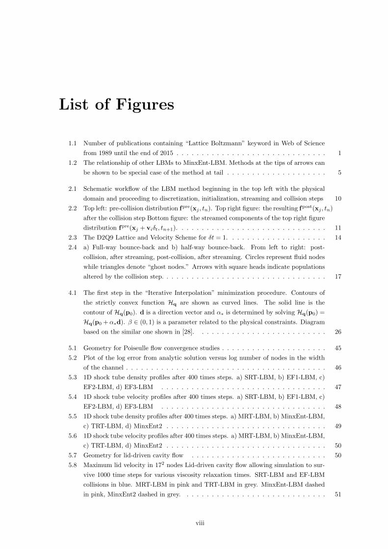
1.1 Number of publications containing “Lattice Boltzmann” keyword in Web of Science
from 1989 until the end of 2015 . . . . . . . . . . . . . . . . . . . . . . . . . . . . . . 1
1.2 The relationship of other LBMs to MinxEnt-LBM. Methods at the tips of arrows can
be shown to be special case of the method at tail . . . . . . . . . . . . . . . . . . . . 5
2.1 Schematic workflow of the LBM method beginning in the top left with the physical
domain and proceeding to discretization, initialization, streaming and collision steps 10
2.2 Top left: pre-collision distribution fpre(xj , tn). Top right figure: the resulting fpost(xj , tn)
after the collision step Bottom figure: the streamed components of the top right figure
distribution fpre(xj + viδt, tn+1). . . . . . . . . . . . . . . . . . . . . . . . . . . . . . 11
2.3 The D2Q9 Lattice and Velocity Scheme for δt = 1. . . . . . . . . . . . . . . . . . . . 14
2.4 a) Full-way bounce-back and b) half-way bounce-back. From left to right: post-
collision, after streaming, post-collision, after streaming. Circles represent fluid nodes
while triangles denote “ghost nodes.” Arrows with square heads indicate populations
altered by the collision step. . . . . . . . . . . . . . . . . . . . . . . . . . . . . . . . . 17
4.1 The first step in the “Iterative Interpolation” minimization procedure. Contours of
the strictly convex function Hq are shown as curved lines. The solid line is the
contour of Hq(p0). d is a direction vector and α∗ is determined by solving Hq(p0) =
Hq(p0 + α∗d). β ∈ (0, 1) is a parameter related to the physical constraints. Diagram
based on the similar one shown in [28]. . . . . . . . . . . . . . . . . . . . . . . . . . 26
5.1 Geometry for Poiseulle flow convergence studies . . . . . . . . . . . . . . . . . . . . . 45
5.2 Plot of the log error from analytic solution versus log number of nodes in the width
of the channel . . . . . . . . . . . . . . . . . . . . . . . . . . . . . . . . . . . . . . . . 46
5.3 1D shock tube density profiles after 400 times steps. a) SRT-LBM, b) EF1-LBM, c)
EF2-LBM, d) EF3-LBM . . . . . . . . . . . . . . . . . . . . . . . . . . . . . . . . . 47
5.4 1D shock tube velocity profiles after 400 times steps. a) SRT-LBM, b) EF1-LBM, c)
EF2-LBM, d) EF3-LBM . . . . . . . . . . . . . . . . . . . . . . . . . . . . . . . . . 48
5.5 1D shock tube density profiles after 400 times steps. a) MRT-LBM, b) MinxEnt-LBM,
c) TRT-LBM, d) MinxEnt2 . . . . . . . . . . . . . . . . . . . . . . . . . . . . . . . . 49
5.6 1D shock tube velocity profiles after 400 times steps. a) MRT-LBM, b) MinxEnt-LBM,
c) TRT-LBM, d) MinxEnt2 . . . . . . . . . . . . . . . . . . . . . . . . . . . . . . . . 50
5.7 Geometry for lid-driven cavity flow . . . . . . . . . . . . . . . . . . . . . . . . . . . 50
5.8 Maximum lid velocity in 172 nodes Lid-driven cavity flow allowing simulation to sur-
vive 1000 time steps for various viscosity relaxation times. SRT-LBM and EF-LBM
collisions in blue. MRT-LBM in pink and TRT-LBM in grey. MinxEnt-LBM dashed
in pink, MinxEnt2 dashed in grey. . . . . . . . . . . . . . . . . . . . . . . . . . . . . 51
viii

5.9 Flow contours of lid-driven cavity flow for Re= 100 with N = 2572. Left-Pressure
deviation, Middle: Stream Function, Right: Vorticity. Top Row: Comsol, Middle
Row: SRT-LBM, Bottom Row: EF3-LBM . . . . . . . . . . . . . . . . . . . . . . . . 53
5.10 Same as Figure 5.9, Re= 400 . . . . . . . . . . . . . . . . . . . . . . . . . . . . . . . 53
5.11 Same as Figure 5.9, Re= 1000 . . . . . . . . . . . . . . . . . . . . . . . . . . . . . . . 54
5.12 Same as Figure 5.9, Top Row: Comsol, Middle Row: MRT-LBM, Bottom Row:
MInxEnt4-LBM . . . . . . . . . . . . . . . . . . . . . . . . . . . . . . . . . . . . . . . 58
5.13 Same as Figure 5.12, Re= 400 . . . . . . . . . . . . . . . . . . . . . . . . . . . . . . . 59
5.14 Same as Figure 5.12, Re= 1000 . . . . . . . . . . . . . . . . . . . . . . . . . . . . . . 60
5.15 Same as Figure 5.9, Top Row: Comsol, Middle Row: TRT-LBM, Bottom Row: Minx-
Ent2 . . . . . . . . . . . . . . . . . . . . . . . . . . . . . . . . . . . . . . . . . . . . . 61
5.16 Same as Figure 5.15, Re= 400 . . . . . . . . . . . . . . . . . . . . . . . . . . . . . . . 62
5.17 Same as Figure 5.15, Re= 1000 . . . . . . . . . . . . . . . . . . . . . . . . . . . . . . 63
ix

Chapter 1
Introduction
The Lattice Boltzmann Method (LBM) is a mesoscale discrete velocity model that has become
an increasingly popular method (see Figure 1.1) for simulating fluid flows, particularly in complex
geometries like porous flow (see [1] for a recent review). It employs a carefully coordinated dis-
cretization of physical space, velocity space and time, to track the evolution of a vector valued mass
expectation distribution, f (whose vector components are called “populations.”) This evolution is
carried out in a cycle of “streaming” and “collision” steps (see §2.1). Historically, the LBM evolved
[2, 3, 4, 5, 6, 7, 8] from the Lattice Gas Automata, or LGA (for an excellent treatment of the LGA
see [9, 10]). The LBM was created to address undesirable features of the LGA such as statistical
noise. Thus, the original interpretation of the LBM was that it was a generalization of the LGA.
The second interpretation of the LBM is that the LBM is a special finite difference form of the
continuous Boltzmann Equation [11, 12, 13, 14]. The finite difference view of the LBM allowed
researchers to explore various aspects of the LBM by performing the discretization using various
quadratures and lattices.
Figure 1.1: Number of publications containing “Lattice Boltzmann” keyword in Web of Science from1989 until the end of 2015
Despite this progress it became clear that the LBM can suffer from numerical instabilities. Ac-
cording to Sterling and Chen,
it is well known among LB researchers that instability problems arise frequently. When
the LB method is viewed as a finite-difference method for solving the continuum discrete-
1

Chapter 1. Introduction 2
velocity Boltzmann equations, it becomes clear that numerical accuracy and stability
issues should be addressed.[15]
Increasing the stability of the LBM became the focus of significant effort. One cause of instability
is that even if the mass expectation populations start positively valued they can become negative
during the course of a typical simulation. As a result, one of the natural places to start to improve
stability was to ensure that all mass expectation populations remained non-negative [16]. Although
this helped, it did not ensure stability [17].
Much of the work done to address the stability issues of the LBM over the last twenty plus years
has been to attempt to endow the Lattice Boltzmann Method with some of the features of LGA.
This is because, despite the flaws of the LGA, it had some built-in advantages. Quoting Boghosian
and co-workers,
One often overlooked advantage of lattice-gas models is their unconditional stability.
By insisting that lattice-gas collisions obey a detailed-balance condition, we are ensured
of the validity of Boltzmann’s H theorem, the fluctuation-dissipation theorem, Onsager
reciprocity, and a host of other critically important properties with macroscopic conse-
quences. [18]
Indeed, a growing number of researchers felt that the lack of unconditional stability (particularly
with thermal Lattice Boltzmann Methods) was due to the lack of a so-called “H-Theorem” for the
LBM.
The classical H-Theorem of Boltzmann in 1872 was a key development in statistical mechanics.
A translation of his original paper is given in [19]. For a gas of spherical particles undergoing
elastic collisions Boltzmann was able to show that given a continuous mass expectation distribution,
f(x,v, t), one could define an H-function,
H[f ] =
∫∫f(x,v, t) ln f(x,v, t) dvdx, (1.1)
which was monotonically non-increasing in time. The thermodynamic entropy is related to this
function by,
Sthermo = −kBH,
where kB is the Boltzmann constant. Using variational methods one can easily verify that the
Maxwell-Boltzmann distribution,
fMB(x,v, t) =ρ
(2πRT )D/2e−|v−u|22RT (1.2)
is the unique minimizer of (1.1) under the physical constraints,
ρ(x, t) =
∫RD
f(x,v, t) dv (1.3)
ρ(x, t) u(x, t) =
∫RD
v f(x,v, t) dv (1.4)
RD
2ρ(x, t)RT (x, t) =
1
2
∫RD
|v − u(x, t)|2 f(x,v, t) dv (1.5)
where D is the physical dimension, R is the specific gas constant, ρ(x, t) is the density at x ∈ RD
and time t ∈ R, u(x, t) is the macroscopic velocity and T (x, t) is the temperature. This has the

Chapter 1. Introduction 3
interpretation that without additional forces or interactions, the velocity distribution of a gas of
elastically colliding particles will evolve into the Maxwell-Boltzmann distribution over time. The
Maxwell-Boltzmann distribution serves as both a stationary state as well as an attractor for the
system.
The Lattice Boltzmann method alternates between “streaming” steps and “collision” steps. In the
collision step, the collision instantaneously replaces the pre-collision mass expectation distribution
fpre(x, t) with a post-collision distribution fpost(x, t). The streaming step then “streams” the post-
collision populations to neighbouring nodes, producing pre-collision expectation distributions at time
t+ ∆t.
The original Single Relaxation Time Lattice Boltzmann Method (SRT-LBM, also called LBGK
LBM) collision step,
fpost(xj , tn) = fpre(xj , tn) +1
τ(f eq(xj , tn)− fpre(xj , tn)) , (1.6)
has a stationary state (called the equilibrium distribution, f eq) that does not serve as an attractor.
In fact, one can easily convince oneself that starting with a seemingly harmless initial state, repeated
application of (1.6) will lead to unbounded growth of f , particularly if some components of fpre are
very different from the corresponding components of f eq . This suggested to some authors that the
LBM should be equipped with an H-Theorem. According to Chen et al,
We point out that the fundamental origin of the instability in [thermal Lattice Boltzmann
models] can be attributed to the violation of a global H-theorem. On the contrary,
[isothermal Lattice Boltzmann models] systems do not suffer from such a problem. [20]
This was expanded upon by Succi,
The violation of the global H-Theorem manifests itself whenever the temperature field
acquires a spatial dependence. On the other hand, though the transition probabilities are
not unity, they become constants in the isothermal LB models, which explains why the
above problem disappears for isothermal LB models. This essential difference between
thermal and isothermal lattice models lies at the heart of the significantly better stability
of the latter. [21]
Even though athermal (without a well defined physical temperature) and isothemral (having
a well defined, uniform, constant temperature) Lattice Boltzmann Methods seemed to be more
stable than their thermal counterparts, a number of researchers still noted instabilities in isothermal
simulations and attributed them to lack of an H-Theorem[22, 18, 23, 24]. Attempts to equip the
LBM with an H-Theorem, or incorporate some notion of entropy, have spanned the last 15 years
and are generally referred to as “entropic methods”.
To equip the LBM with an H-Theorem one must provide a functional (hereafter called an “en-
tropy”) that is monotonically decreasing in time. In addition, simulations using the corresponding
equilibrium and collision step must produce in physically accurate results.
The first attempts to equip the LBM with an H-Theorem were to retain the SRT-LBM collision
step (1.6) and instead of using the original and most popular polynomial equilibrium [8], (2.16), one
chooses an equilibrium distribution that minimizes a chosen entropy functional, subject to constraints
that ensure proper dynamics [25, 26, 27]. Karlin et al [28] proposed that any such entropy should be
convex and when the corresponding equilibrium is used in the SRT-LBM collision, (1.6) one must
recover the Navier-Stokes equations up to second order in the macroscopic velocity, u.
Entropy functions that satisfy these requirements are called “perfect entropy functions.” Though
Karlin et al. were able to find such a perfect entropy function for 2 cases (a 1 dimensional, 3 velocity

Chapter 1. Introduction 4
lattice, and a 2 dimensional 9 velocity lattice), finding an entropy function for a given lattice is
non-trivial in general and in some situations may be impossible. Also, Wagner [29] showed that one
cannot find a perfect entropy function for Lattice Boltzmann implementations that use an equilibrium
that is a polynomial in u.
Requiring that the equilibrium be a polynomial was sufficient (but not necessary) to ensure that
model would be Galilean invariant, which was one of the requirements for LBMs with H-Theorems
set by Succi et al. in [21]. (However, non-polynomial equilibrium Galilean invariant models were
suggested by Boghosian and coworkers [23, 30]). The other two requirements outlined in [21] were
that the equilibrium should be realizable (bounded between 0 and 1) and also solvable (expressible
as an explicit function of the local macroscopic properties).
All of the above requirements put tremendous restrictions on finding a suitable equilibrium while
keeping the SRT-LBM collision step. An alternative path to equipping the LBM with an H-Theorem
would be to find a novel collision step that is not the SRT collision (1.6) . The most popular of
these alternative collision steps is the Entropic Lattice Boltzmann Method (ELBM) and was first
described by Karlin et al. in 1999 [28]. This method constructs a collision step based on knowledge
of the entropy function only. Though the collision step may include an equilibrium distribution,
in general the ELBM circumvents the need for finding an equilibrium distribution with specific
attributes. Early work with the ELBM [22, 31] used the perfect entropy functions developed in [28]
but eventually a more popular entropy function based on Boltzmann’s original H-function (1.1) was
suggested [32],
S[f ] =∑i
fi lnfiWi
, (1.7)
where fi is the ith component of f and the Wi are weights that depend on the choice of lattice (for
example, see §2.1.6). An explicit corresponding equilibrium for this entropy function that conserves
mass and momentum can in fact be found [32] (see (5.2)). Since then many tests of the ELBM
collision step have used this function in some manner (for an example [33, 34, 35], and others). An
excellent review of the early work on equipping the LBM with an H-Theorem can be found in [21]
and [36].
In addition to attempts to equip the LBM with an H-Theorem, other entropic methods have
been explored such as non-equilibrium entropy limiters [37], and Ehrenfests’ coarse-graining [38, 39,
40]. The assumption that the LBM should (or even could incorporate entropic principles was not
universally accepted. A wide range of other attempts have been made to improve the stability of the
LBM. Chief among them is the Multiple Relaxation Time Lattice Boltzmann Method (MRT-LBM)
[41, 42, 43, 44, 45, 46, 47, 48]. There is a bit of a split in the LBM community, between the advocates
of entropic methods, and advocates of MRT-LBM.
In fact, critics of entropic methods claim that there are many issues with entropic methods. One
major issue is that they can be comparatively computationally expensive. Some authors claim that
the benefits of entropic methods may be overstated [49, 39, 50, 51], impossible to implement in
certain conditions [52], and impractical [53].
Despite the popularity of entropic methods and MRT-LBM methods, a host of other techniques
claim to increase stability as well. These include changing the boundary conditions [54, 55],“link-
based” two-relaxation time-methods [56, 57, 58], least squares finite element LBM [59], regularized
LBM [60], additional velocities [61], “Onsager-like” relation collision step [62], double MRT-LBM
(for thermal flows) [63]. However, we will limit our focus on entropic methods and relaxation-time

Chapter 1. Introduction 5
methods.
We share the view that a notion of entropy plays an important role in the stability of the LBM
and that entropy violations are a cause of numerical instabilities. In addition we claim that stability
improvements from MRT-LBM methods and other entropic methods are manifestations of the same
underlying principle, and that these approaches are not mutually exclusive and can, in fact, be
unified.
The LBM has been largely used for fluid flow applications (though some non-fluid applications do
exist, for example [64]) and for near-equilibrium flows in particular. Indeed, the relationship between
the relaxation times used in implementations of the LBM and simulated fluid properties is typically
derived by applying a Chapman-Enskog analysis and assuming near-equilibrium, low Mach number
and a small Knudsen number. Equations derived from a Chapman-Enskog analysis are compared
to the presupposed governing equations (the Navier-Stokes equations) and it is only then that one
is able to specify values for some relaxation times. For example, see [12]. This leads one to wonder
if the LBM could be used in a wider range of non-fluid and/or far from equilibrium applications
without an a priori knowledge of the governing macroscopic equations.
In this thesis we describe a novel, third interpretation of the LBM. This new interpretation
is based on the Principle of Minimum Discrimination Information (or Minimum Cross Entropy)
MinxEnt. We will call this LBM based on MinxEnt, “MinxEnt-LBM” (see Figure 1.2).
Principle of Minimum Discrimination Information (MinxEnt)
Entropic Methods
MinxEnt-LBM
ELBM
EF-LBM
MRT-LBM
TRT-LBM
SRT-LBM
Relaxation Time Methods
Figure 1.2: The relationship of other LBMs to MinxEnt-LBM. Methods at the tips of arrows can beshown to be special case of the method at tail
Further, we will show that MRT-LBM, entropic LBM (ELBM) and Ehrenfest Step LBM (EF-
LBM) [39, 40, 65] are all different, simplified approximations of the MinxEnt-LBM scheme. We
compare the MinxEnt-LBM scheme to these other LBM schemes for benchmark problems: 1-D
shock tube and 2D lid-driven cavity flow.
Finally, in constructing the MinxEnt-LBM framework we will see how it naturally suggests av-

Chapter 1. Introduction 6
enues to allow the method to be extended beyond fluid flow applications and to systems in which
the governing macroscopic equations are not known ahead of time. This is possible because the
MinxEnt-LBM framework is built on constrained optimization rather than presupposed governing
equations. One can envision simulating systems where constraints are known, but the macroscopic
evolution equations are not.
This thesis is organized in the following way: the LBM, and some of its current variations
are described in Section 2. Section 3 outlines the foundation of our method, MinxEnt. Section
4 outlines the MinxEnt-LBM framework and includes the unification of other LBMs as different
approximations of MinxEnt-LBM. Section 5 gives some numerical results and Section 6 offers final
thoughts and future work.

Chapter 2
Lattice Boltzmann Methods
In kinetic theory [66], the evolution of macroscopic properties often involves understanding the
behaviour of a mass expectation density, f , (hereafter called a “distribution”),
f = f(x,v, t).
For example in a fluid simulation, knowledge of the mass expectation distribution allows one to
calculate macroscopic properties of the fluid such as density, momentum and temperature,
ρ(x, t) =
∫RD
f(x,v, t) dv (2.1)
ρ(x, t) u(x, t) =
∫RD
v f(x,v, t) dv (2.2)
RD
2ρ(x, t)RT (x, t) =
1
2
∫RD
|v − u(x, t)|2 f(x,v, t) dv (2.3)
The usual kinetic theory approach to calculating the evolution of f is based on solving the
Boltzmann Equation (BE) [66]:
∂f
∂t+ v · ∇xf +
F
m· ∇vf = C[f ] (2.4)
where F is the external force and C[f ] is the change in f due to collisions (typically called the
“collision term”). In practice, using computers to approximate solutions of the BE is very challenging
because of the collision term.
Understanding f is also the fundamental objective of the Lattice Boltzmann Method (LBM). In
fact it has been shown that using various approximations of the collision term while employing a
specific discretization of the BE leads to versions of the LBM [11, 12, 13, 67, 14].
In this section we will describe the Lattice Boltzmann Method, as well as outline some of the
variants that can be found in the literature. For a more detailed explanation of the connection
between f and macroscopic properties of a system, see Appendix A.
2.1 LBM Simulation Procedure
Consider a finite time step, δt. Given a distribution f at time t we approximate f at time t+ δt with
a two-step process; a “collision step” followed by a local “streaming step.”
7

Chapter 2. Lattice Boltzmann Methods 8
In the instantaneous collision step, a local operator (denoted ∆) takes fpre = f at time t and
maps it to fpost at time t:
Collision Step: fpost(x,v, t) = ∆[fpre(x,v, t)],
In this context, “local” means local in x: the post-collision distribution at position x is determined
by the pre-collision distribution at position x only — the pre-collision distributions at points other
than x have no effect. This is one of the powerful features of LBM; it is very suitable for parallel
computation.
Given the post-collision distributions, fpost, at time t at all locations x, constructs pre-collision
distributions at time t + δt by “sending components” of the fpost to neighbouring locations in the
natural manner determined by their velocities
Streaming Step: fpre(x + v δt,v, t+ δt) = fpost(x,v, t),
The streaming step moves the values of the distribution unchanged from position to position according
to their velocities. This is usually known as “free streaming” or “free transport.” The fact that
distributions do not evolve by free transport is addressed by the collision step.
A defining feature of the LBM is the discretization of space into a lattice, Λ, with a commensurate
discretization of the velocities. Let x,v ∈ RD be a position and a velocity respectively. If the system
occupies a region of physical space, Ω ⊂ RD then x ∈ Ω. The velocity, v, is unconstrained: v ∈ RD.
The LBM tracks the evolution of a discrete, vector-valued distribution, f(x, t), which is defined at
only a regular, uniform, discrete set of positions and velocities. That is,
x = xj ,∈ Ω ∩ Λ
where Λ is a lattice in RD and
v = vi ∈ v1,v2, . . . ,vb
where v1,v2, . . . ,vb is the set of allowed velocities. Given a time-step δt, the velocities must
satisfy xj + vi δt ∈ Λ for all i ∈ 1, . . . , b and all xj ∈ Ω ∩ Λ in order for the velocity discretization
to be compatible with Λ at δt. The vector-valued distribution, f(xj , t) is related to the continuous
distribution by components:
fi(xj , t) ≈ f(xj ,vi, t)
A typical LBM simulation would proceed as follows, making note that the order of streaming
and collision step does not matter in practice:
1. Discretize space, velocity, and time: Above, x ∈ Ω ⊂ RD, v ∈ RD, t ∈ R, and the mass
expectation distribution, f , takes on values in R. As discussed in detail in §2.1.6, a finite set of
velocities vi, i ∈ 1, . . . , b is chosen; see Figure 2.3 for an example of a lattice in R2 and set of
nine velocities. A fixed time step, δt, is also chosen with time discretized accordingly: tn = n δt
with n ∈ N. A compatible lattice Λ is constructed and then intersected with Ω; this results in
a discrete set of points xj ∈ Λ ∩ Ω. The distance between nearest neighbour nodes is uniform
and denoted δx. How this discretiztion is done is an open topic in LBM research. For example,
one may ask about the connection between the number of permissible velocities and accuracy
of the method. Because of the discretization of velocity, the distribution f(xj , ·, tn) : RD → Ris approximated with a vector f(xj , tn) ∈ Rb.
2. Initialize distributions: At t = 0, at each node xj , all b components of the (now discrete)

Chapter 2. Lattice Boltzmann Methods 9
distribution fpre(xj , 0) are assigned, in such a way that the macroscopic initial conditions,
such as density, mean velocity, etc, at xj are satisfied.
3. Compute macroscopic quantities: Using fpre(xj , tn), macroscopic quantities such as density
and mean velocity, are then calculated using discretized versions of (2.1) - (2.3) at each node
xj (see §2.1.6).
4. Compute local equilibrium: Using the macroscopic quantities, calculate a local “equilibrium
distribution” f eq(xj , tn) at each node xj ; see §2.1.1 and §2.1.6.
5. Collision Step: The pre-collision and equilibrium distributions are used to define the post-
collision distribution at time tn:
fpost(xj , tn) = ∆[fpre(xj , tn), f eq(xj , tn)]
for all xj ∈ Λ∩Ω. See §2.1.2 to §2.1.5 for a discussion of some standard choices for the collision
operator ∆.
6. Streaming step: At every node xj ∈ Λ ∩ Ω, each component of the distribution at time tn is
streamed according to
fprei (xj + vi δt, tn+1) = fpost
i (xj , tn) ∀i ∈ 1, . . . , b (2.5)
to create the pre-collision distribution fpre at time tn+1. Implicit in (2.5) is that xj+vi δt = xj′
for some j′; this requires that the lattice Λ and the velocity discretization are compatible (see
§2.1.6).
7. Iterate: Having determined fpost(xj , tn+1) at all nodes, repeat steps 3-6 to determine fpre(xj , tn+2)
and so on.
A schematic workflow of the LBM is shown in Figure 2.1
Boundary conditions are imposed as needed either during the collision step, or the streaming
step; see §2.1.7.
2.1.1 Equilibrium Distributions
Here we give two popular choices for the equilibrium distribution.
Maxwell-Boltzmann Based Equilibrium
For systems involving classical fluid particles, the most widely used equilibrium distribution [8] is
based on the continuous Maxwell-Boltzmann Distribution:
f eq(x,v, t) =ρ
(2πRT )D/2e−|v−u|22RT . (2.6)
It should also be noted that for other types of fluids (quantum fluids for example) the Maxwell-
Boltzmann Distribution may not be the appropriate equilibrium for that system.
Entropy Based Equilibrium
As discussed in the introduction, one path to equipping an LBM with an H-Theorem is to choose an
equilibrium that maximizes an entropy function subject to constraints. In an athermal simulation

Chapter 2. Lattice Boltzmann Methods 10
Converged
Physical Domain Discretized Initialized
Post Stream
Macroscopic Quantities
Post Collision
Stream
Stream
Locally collide using: MRT, ELBM, MinxEnt, or other rule
Figure 2.1: Schematic workflow of the LBM method beginning in the top left with the physicaldomain and proceeding to discretization, initialization, streaming and collision steps
these constraints are conservation of mass and momentum,
ρ(x, t) =
∫RD
f(x,v, t) dv
ρ(x, t) u(x, t) =
∫RD
v f(x,v, t) dv
The resulting equilibrium distribution which maximizes the entropy subject to hydrodynamic
constraints will be discussed in §5.1.1.
2.1.2 Collision Step: Single Relaxation Time (SRT-LBM)
The collision step accounts for changes to the components of the distribution arising from collision
between fluid particles.
The first, most popular and simplest collision step is based the linearization of the kinetic collision
term [3, 4] and further approximating by assuming a single relaxation time τ [5]:
∆[fpre(xj , tn), f eq(xj , tn)] = fpre(xj , tn) +1
τ(f eq(xj , tn)− fpre(xj , tn)) . (2.7)
f eq(xj , tn) is an equilibrium distribution (see §2.1.1) and τ is some predetermined relaxation time
that is related to the fluid viscosity; this relationship is lattice dependent and is discussed for a
specific lattice in §5.1.2 . This single relaxation time approach was made more popular in [8] and
assumed the name Lattice BGK (LBGK) owing to its similarity to the Bhatnagar-Gross-Krook
kinetic equation [68]. For this reason it is common in the literature to refer to LBMs using the single

Chapter 2. Lattice Boltzmann Methods 11
Collision Step
Streaming Step
Figure 2.2: Top left: pre-collision distribution fpre(xj , tn). Top right figure: the resulting fpost(xj , tn)after the collision step Bottom figure: the streamed components of the top right figure distributionfpre(xj + viδt, tn+1).
relaxation time collision step as “LBGK.”
2.1.3 Collision Step: Multiple Relaxation Time (MRT-LBM)
Historically, two major problems researchers encountered when implementing the SRT-LBM were
that
1. one couldn’t specify the Prandtl number for a simulation
2. numerical instabilities
The Prandtl number is the ratio of a fluid’s kinematic viscosity and its thermal diffusivity; fluids can
have the same kinematic viscosity but have different Prandtl numbers. Owing to its single adjustable
parameter (τ), SRT-LBM fixes both the kinematic viscosity and the Prandtl number. In an attempt
to rectify this issue and the stability problems, researchers returned to the more general linearized
collision term of [3, 4] which allowed for multiple relaxation times during the collision step [41, 42,
43, 44, 45, 46, 47, 48]. This is accomplished via the collision operator:
∆[fpre(xj , tn), f eq(xj , tn)] = fpre(xj , tn) + T−1BT (f eq(xj , tn)− fpre(xj , tn)) (2.8)
where B is a diagonal matrix of relaxation times and T is an invertible matrix taking the vector f
into “moment space.” Note that the SRT-LBM collision step (2.7) can be recovered from the MRT-
LBM collision by assuming B = 1τ I. The class of “Two Relaxation Time” (TRT-LBM) collision

Chapter 2. Lattice Boltzmann Methods 12
steps was suggested by Ginzburg et al. [69] and is related to accuracy at boundaries [70, 53]. In the
TRT-LBM, the entries of B can take only one of two values.
2.1.4 Collision Step: Entropic Lattice Boltzmann Method (ELBM)
Given a convex entropy function, S(f), (sometimes written as H in the literature) and “bare col-
lision,” ∆ (which may, or may not involve an equilibrium distribution) the ELBM collision step is
designed to lower the value of S and is carried out in two steps:
1. Calculate α where α satisfies:
S (fpre) = S (fpre + α∆)
2. Compute the collision
fpost(xj , tn) = fpre(xj , tn) + βα∆(xj , tn)
where 0 < β < 1 is a number related to the kinematic viscosity of the fluid. Constructing the
collision step in this way ensures that the entropy of the post-collision distribution is less than the
pre-collision distribution. Note that the value of α must be calculated (if possible) at every xj and
every tn; this slows down the procedure.
2.1.5 Collision Step: SRT-LBM with Ehrenfest Steps (EF-LBM)
Another attempt to stabilize the LBM using entropic ideas is based on Ehrenfest coarse graining
[71]. The EF-LBM collision equips the LBM with an entropy limiter which monitors the simulation
for spatial points at which some type of local entropic criteria is violated [39]. This approach has
been shown to be successful in reducing instabilities in 1-D shock tube simulations [39, 40, 49, 50,
37, 51] and 2D lid driven cavity flow [51].
Similar to the ELBM, EF-LBM wants the value of a given an entropy function, S(f), to decrease
during the collision step. However, rather than insist S always decreases EF-LBM instead monitors
the local nonequilibrium entropy, ∆S, defined as,
∆S(fpre) ≡ S(f eq)− S(fpre). (2.9)
∆S serves as an indicator of locations that the collision step may increase S. If ∆S is below some
threshold, a regular SRT-LBM (2.7) collision step is taken. Otherwise, if the threshold is exceeded,
the collision step is altered at the offending location. For example the collision step in the popular
version of EF-LBM is,
∆[fpre(xj , tn),f eq(xj , tn)] =fpre(xj , tn) + 1τ (f eq(xj , tn)− fpre(xj , tn)) if ∆S (fpre) < tolerance
fpre(xj , tn) + 12τ (f eq(xj , tn)− fpre(xj , tn)) otherwise.
(2.10)
We can see from (2.10) that if ∆S is above tolerance, the approach of EF-LBM is to reduce the
change in f that occurs during collision step, effectively making the collision step more “gentle.” It
is also interesting to note that if τ ≈ 12 , the effect of using (2.10) is to set fpost to approximately the
equilibrium. This is important because it is well known that numerical instabilities in SRT-LBM
grow as τ nears 12 .

Chapter 2. Lattice Boltzmann Methods 13
2.1.6 Discretization: D2Q9 Scheme Example
How the lattice Λ and the set of admissible velocities are chosen crucially impacts the accuracy of
the LBM. Typically the scheme is chosen for the accurate calculation of the hydrodynamic moments
of the flow, at least for the case of the Maxwell-Boltzmann based equilibrium distribution (2.6).
Consider the expected value of φ for some function φ(v):∫RD
f eq(x,v, t)φ(v) dv =ρ
(2πRT )D/2
∫RD
e−|v−u|22RT φ(v) dv (2.11)
=ρ
(2πRT )D/2e−|u|22RT
∫RD
e−|v|22RT e
v·uRT φ(v) dv
=ρ
(2πRT )D/2e−|u|22RT
∫Re−
v21
2RT . . .
∫Re−
v2D
2RT ev·uRT φ(v) dvD . . . dv1
=ρ
(2πRT )D/2e−|u|22RT
∫Re−
v21
2RT . . .
∫Re−
v2D
2RT φ(v) dvD . . . dv1 (2.12)
where φ(v) = exp(v ·(u/(RT )))φ(v). Each of the D integrals in (2.12) is suitable for Gauss-Hermite
quadrature. Consider the innermost integral
ρ
(2πRT )1/2
∫Re−
v2D
2RT φ(v) dvD. (2.13)
We discretize the Dth dimension of the velocity space as (vD)i =√
2RTξi where the ξi are the zeros
of the degree 3 Hermite polynomials; ξi ∈ −√
62 , 0,
√6
2 . The associated weights are given by the
1-D wi ∈ 16 ,
23 ,
16 respectively.
Thus,
ρ
(2πRT )1/2
∫Re−
v2D
2RT φ(v) dvD ≈3∑i=1
wi φ(v1, . . . , vD−1, (vD)i)
where (vD)i ∈ −√
3RT, 0,√
3RT. The two innermost integrals are then approximated as
ρ
(2πRT )
∫Re−
v2D−12RT
∫Re−
v2D
2RT φ(v) dvD dvD−1
≈3∑j=1
wj
3∑i=1
wi φ(v1, . . . , vD−2, (vD−1)j , (vD)i),
where,
(vD−1)j =√
2RTξj
and
ξj ∈
−√
6
2, 0
√6
2
.
Proceeding in this way, the integral (2.12) over RD would be approximated as the sum of 3D terms.
Each term would involve a weight Wi which is the product of D one dimensional weights. The
velocity space RD would be discretized using 3D vectors vi; the components of vi take values in
−√
3RT, 0,√
3RT.For integrals over R2, this leads to the popular “D2Q9” (two dimensions, 9 velocities) scheme.
shown in Figure 2.3. Λ is the square lattice in R2 and there are nine admissible velocities shown
in Figure 2.3; the admissible velocities are shown at the central node. The velocities v1,v2,v3 and
v4 all have the same magnitude and point towards the nearest neighbours of the central node. The
velocities v5,v6,v7 and v8 also all have the same magnitude and point towards the next-nearest

Chapter 2. Lattice Boltzmann Methods 14
neighbours. The ninth velocity v9 is 0.
Figure 2.3: The D2Q9 Lattice and Velocity Scheme for δt = 1.
The components of the velocities and weights are given in Table 2.1.
Table 2.1: D2Q9 Velocity Scheme: c =√
3RT
i 1 2 3 4 5 6 7 8 9
vi (c,0) (0,c) (-c,0) (0,-c) (c,c) (-c,c) (-c,-c) (c,-c) (0,0)
Wi19
19
19
19
136
136
136
136
49
Recalling that the goal was to approximate integrals (2.11) of the continuous equilibrium distri-
bution (2.6), we have
∫R2
f eq(x,v, t)φ(v) dv ≈ ρ9∑i=1
Wie2vi·u−|u|
2
2RT φ(vi) =
9∑i=1
f eqi φ(vi) (2.14)
where we’ve defined the discrete equilibrium distribution, f eq, via
f eqi := ρWi e
2vi·u−|u|2
2RT . (2.15)
Note that, just like the continuous equilibrium distribution (2.6), the discrete equilibrium distribution
f eq is a function of v and depends on the macroscopic quantities ρ(x, t), u(x, t), and T (x, t). However,
in an athermal scheme, we are free to choose a fixed T and thus will choose it to simplify our velocity
scheme. For example, choosing T so that RT = 1 sets c =√
3.
Now, since our quadrature is a direct product of 2 Gauss-Hermite quadratures based on three

Chapter 2. Lattice Boltzmann Methods 15
points, the bound on the error of each integration will involve the sixth derivative of,
φ(v) = e(v·u/(RT )) φ(v)
with respect to v. If we are only interested in expectation values of macroscopic quantities such
as density and velocity (or temperature if using a thermal LBM) then the function φ(v) will be
a polynomial of degree two or less. However, even though φ(v) is a low degree polynomial the
exp((v·u)/(RT ) term in φ(v) causes φ not to be a polynomial. This leads to errors in the integration.
To address this problem one could add more points for the Gauss-Hermite quadrature. However, if
one used more than three points to discretize each component of the velocity this would not yield a
velocity discretization that led to a lattice in x [72] requiring additional effort such as those outlined
in [73].
However, if one assumes a “low Mach number” approximation, |u|√RT 1, for the the continuous
equilibrium distribution (2.6) then,
f eq ≈ ρ
(2πRT )D/2e−
v2
2RT
1− |u|
2
2RT+
v · uRT
+(v · u)2
2(RT )2
(2.16)
This is the typical approach taken in most LBM simulations and in this case,
φ(v) =
1− |u|
2
2RT+
v · uRT
+(v · u)2
2(RT )2
φ(v)
which guarantees the integration is exact for φ(v) of degree 2 or less.
In the low mach number approximation the expression for the moments (2.14) would still hold
but with a different discrete form of the equilibrium. Rather than using (2.15), one would use
f eqi := ρWi
1− |u|
2
2RT+
vi · uRT
+(vi · u)2
2(RT )2
. (2.17)
The scheme in Table 2.1 was made to ensure the accuracy of integration involving the equilibrium
distribution. For integrations involving a general distribution, f(x,v, t), we manipulate the hydro-
dynamic integral into a form suitable for Gauss-Hermite quadrature and apply the discritization
motivated above: ∫f(x,v, t)φ(v) dv =
∫ω(v)
f(x,v, t)
ω(v)φ(v) dv
≈9∑i=1
Wif(x,vi, t)
ω(vi)φ(vi)
where
ω(v) =1
(2πRT )D/2e−|v|22RT . (2.18)
Note that ω is the continuous Maxwell-Boltzmann distribution with unit mass and zero mean velocity.
As is typically done, we can define a discrete distribution f(x, t) from the continuous distribution
f(x,v, t) via
fi(x, t) = Wif(x,vi, t)
ω(vi)i ∈ 1, 2, . . . , 9. (2.19)
With this notation, in two dimensions the moment based on the continuous distribution f is approx-

Chapter 2. Lattice Boltzmann Methods 16
imated as: ∫f(x,v, t)φ(v) dv ≈
9∑i=1
fi(x, t) φ(vi) (2.20)
If the continuous distribution f(x,v, t) equals ω(v) — that is if f is the Maxwell-Boltzman distri-
bution with unit mass and zero mean velocity — then the corresponding discrete distribution (2.19)
is W. That is, the weights we use in the Gauss-Hermite quadrature are the discrete distribution for
ω(v) as given by (2.18).
It is again worth repeating that since the discretization was chosen to minimize integration error
involving f eq. This means that if a given distribution f is sufficiently far from f eq the integration
accuracy may be quite poor.
In D2Q9 the density, momentum and temperature, (2.1)-(2.3), are calculated from the discrete
distribution f via,
ρ(xj , tn) =
9∑i=1
f(xj , tn) (2.21)
ρ(xj , tn) u(xj , tn) =
9∑i=1
f(xj , tn)vi (2.22)
2.1.7 Boundary Conditions
We call a node xj ∈ Λ∩Ω an “internal node” if the neighbouring nodes involved in the streaming step
are all in Λ∩Ω. At such nodes, the evolution of the distribution function follows the aforementioned
procedure: a local collision step followed by streaming step that constructs fpre from the components
of fpost at neighbouring nodes. After the streaming step the internal node has a complete distribution
with all components determined: see Figure 2.2b. We call a node xj a “boundary node” if any
neighbouring nodes required for the streaming step are not in xj ∈ Λ ∩ Ω. For such a node the
streaming step results in some of the components of the distribution not being determined: see
Figures 2.4b.
To rectify this situation, a number of methods have been devised to implement various types of
boundary conditions. How to implement boundary conditions that are accurate and efficient is a
very active area of research for the LBM see [74, 75, 76, 77, 78, 79] amongst others.
No-Slip Boundary Conditions: stationary boundary
No-slip boundary conditions are imposed to ensure that the macroscopic fluid velocity at the bound-
ary equals the velocity of the boundary itself. If the boundary is stationary then the mean velocity
of the fluid at the boundary should be 0. Due to their simplicity, the most popular methods to
impose no-slip boundary conditions for a stationary boundary are the “bounce-back” schemes.
Let xb be a boundary node. After the streaming step fpre(xb, t+δt) is “missing” some components
because it is a boundary node. That is, fprei (xb, t + δt) is undefined because xb − viδt 6∈ Λ ∩ Ω and
so there is no fposti (xb − viδt). If the “opposite” node xb + viδt is in Λ ∩ Ω then the bounce-back
scheme is to define fprei (xb, t + δt) to be fpre
i(xb, t + δt) where i is the index of the velocity vector
that is opposite to the velocity indexed by i. That is, vi = −vi.
The bounce-back schemes typically come in two classes, full-way bounce-back and half-way
bounce-back. The implementation of these bounce-back rules varies, but a common implementa-
tion would be to provide auxiliary nodes (sometimes called “ghost nodes” or “solid nodes”) that are
not part of the fluid domain but allow for distributions to be streamed to and from them. In such
auxiliary node implementations, full-way bounce-back can be implemented by treating the auxiliary

Chapter 2. Lattice Boltzmann Methods 17
After Stream: After Stream:Post-Collision/Pre-Stream: Post-Collision/Pre-Stream:
Post-Collision/Pre-Stream:
a)
b)After Stream: Post-Collision/Pre-Stream: After Stream:
Figure 2.4: a) Full-way bounce-back and b) half-way bounce-back. From left to right: post-collision,after streaming, post-collision, after streaming. Circles represent fluid nodes while triangles denote“ghost nodes.” Arrows with square heads indicate populations altered by the collision step.
nodes as fluid nodes, except that the usual collision step at the auxiliary nodes is replaced by an
operation that switches the direction of all the components. That is, the only difference between an
auxiliary node and a fluid node is the collision step. Alternatively, for the half-way bounce-back,
the collision step at the auxiliary nodes is replaced by an operation that switches the direction
of all components and then immediately streams the missing components back to the fluid node.
No collision step is necessary at the auxiliary nodes. For both full-way bounce-back and half-way
bounce-back, the actual physical location of the boundary is somewhere between the fluid node and
its neighbouring auxiliary node. See Figure 2.4. It can be shown [70, 53] that the actual location of
the physical boundary (and thus the accuracy of the method) is crucially linked to the values of the
relaxation times.
No-Slip Boundary Conditions: moving boundary
In the case of a moving boundary, the no-slip boundary condition ensures that the mean velocity of
the fluid at the boundary equals the velocity of the boundary. A simple way to implement a fixed
velocity boundary is to place nodes on the boundary and to use a collision step that simply defines
fpost to be the equilibrium that has the desired macroscopic quantities. We will use this method in
this thesis. One should note however that even though simple and effective, setting the distribution
to the equilibrium at the boundary may not be appropriate. One reason for this is because having
the fluid at equilibrium may not reflect the actual physical conditions at the boundary (although
the boundary will have the correct macroscopic density and momentum). Other implementations
of boundary conditions are possible, see for example [79]. Since our study focuses on comparing
the performance of different collision step implementations, the absolute accuracy of the boundary
condition implementations is not our immediate concern. Of course, we do use the same boundary
conditions for all of our simulations for the sake of consistency.
Now that a typical Lattice Boltzmann simulation procedure has been outlined, we turn our
attention to our MinxEnt-LBM procedure, beginning by its foundations in information theory.

Chapter 3
Principle of Minimum
Discrimination Information
(MinxEnt)
Having given a rough description of the general LBM in §2, we now turn to our specific contribution:
the MinxEnt collision step. It comes from an information theoretic approach which we now discuss.
One of the major appeals of the Lattice Boltzmann Method is that it is based on statistical
mechanics rather than on tracking individual particles (as is done in other methods like Molecular
Dynamics simulations) or solving partial differential equations. The LBM accomplishes this by
tracking the evolution of mass expectation distributions with specific velocities and reconstructing
macroscopic properties from them.
In Appendix A we show how the mass expectation distribution is directly related to probability
distributions which describe probabilities of finding particles with certain properties. With this
relationship in mind we take the approach that the fundamental quantity of interest should be
these probability distributions conditioned at a specific point in space and time. That is, we wish
to understand p(x,v, t): the probability of finding a particle with velocity v given that we are at
location x at time t. In Appendix A we show the relationship between f and p (and thus also
between their corresponding discretized versions) is given by,
f(xj , t) = ρ(xj , t) p(xj , t). (3.1)
In this way, determining the f required by the LBM is equivalent to determining p.
The question then becomes: how should one collide a discrete probability distribution ppre to
arrive at ppost? We propose a new way of defining a collision operator to use in the LBM: by
appealing to the Principle of Maximum Entropy (MaxEnt) as described by Jaynes in his seminal
paper from 1957 [80].
In [80], Jaynes makes a connection between research done by Information Theory pioneer Shannon
in his 1948 book [81] and the field of statistical mechanics championed almost 75 years earlier
by Boltzmann and others. To make the connection between Information Theory and statistical
mechanics, Jaynes argues that,
previously one constructed a theory based on equations of motion and supplemented by
additional hypothesis of ergodicity, metric transitivity or equal a priori probability, and
the identification of entropy was made only at the end, by comparison of the resulting
18

Chapter 3. Principle of Minimum Discrimination Information (MinxEnt) 19
equations with the laws of phenomenological thermodynamics. Now however, we can take
entropy as our starting concept and the fact that a probability distribution maximizes
the entropy subject to certain constraints becomes the central fact which justifies the use
of that distribution for inference.
Jaynes goes on to point out that, at the time, the objectivists’ view of probability was that it
was an objective property of the system and that, in principle, it was verifiable in every detail. From
this perspective the goal of the observer was to simply figure out the probability distribution which
Nature follows. On the other hand, the subjectivist point of view of probability was that it was not
an emergent property of a system, rather it was a measure of the ignorance of the observer. That, in
some way, probabilities gave us the tool to measure how uncertain we are of the outcome of a process.
It is from this viewpoint that Jaynes makes the connection to Shannon’s work in information theory.
Shannon wished to quantify the minimum amount of data one would need to transmit in order
to send a message. He asked “how uncertain of the message would you be if you only received a
certain amount of data?” To answer this, Shannon needed to quantify the amount of uncertainty
in a received alphabet character. For example, if one receives an English ‘q’, there is a high prob-
ability that the next letter will be an English ’u’. In this way, receiving an English ‘q’ contained
more “information” than did receiving an English ‘t’. In other words Shannon was looking for a
way to quantify what our intuition told us; we are more “certain” of the outcome of a process if
the corresponding probability distribution is sharply peaked and less certain of the outcome if the
corresponding probability distribution was broadly spread.
Suppose we have a probability distribution of n discrete possible outcomes of an event, p1, p2, ..., pn.
Shannon sought a function H such that,
1. The function should be non-negative: H(p1, p2, ..., pn) ≥ 0
2. The function H(p1, p2, ..., pn) should be lower for probability distributions associated with
greater certainty in the outcome, and higher for probability distributions corresponding to
more uncertain outcomes. In particular H should be maximized when all outcomes are equally
likely: pi = pj ,∀i 6= j (that is, the state of maximum uncertainty).
3. The function should be additive for independent sources of uncertainty. That is, suppose pB
is the probability of an independent event B also occurring. This requirement insists that,
H(p1, p2, ..., pn, pB) = H(p1, p2, ..., pn) +H(pB)
4. The function should be continuous and symmetric in all pi
Shannon found the function,
H(p1, p2, ..., pn) = −Kn∑i=1
pi ln pi (3.2)
satisfied all four criteria. Here K is an arbitrary constant. He called it the Information Entropy due
to its similarities to thermodynamic entropy. It is now usually called the “Shannon Entropy;” the
quantum version is usually called the “von Neumann Entropy”. It was proven by Khinchin in 1957
[82] that (3.2) was in fact the only function that satisfied the four desired properties.
Jaynes showed the connection between Shannon Entropy and thermodynamic entropy and, more
importantly, proved that statistical mechanics is a result of maximizing the Shannon Entropy subject
to physical constraints. This was in direct contrast to the current view at the time which was that

Chapter 3. Principle of Minimum Discrimination Information (MinxEnt) 20
entropy was an outcome of statistical mechanics, not the foundation on which it stood. Jaynes’
approach put statistical mechanics on firmer axiomatic ground. In his concluding paragraph Jaynes
wrote,
The essential point in the arguments presented above is that we accept the von-Neumann-
Shannon expression for entropy, very literally, as a measure of the amount of uncertainty
represented by a probability distribution; thus entropy becomes the primitive concept
with which we work, more fundamental even than energy. If in addition we reinterpret
the prediction problem of statistical mechanics in the subjective sense, we can derive
the usual relations in a very elementary way without any consideration of ensembles or
appeal to the usual arguments concerning ergodicity or equal a priori probabilities. The
principles and mathematical methods of statistical mechanics are seen to be of much
more general applicability than conventional arguments would lead one to suppose. In
the problem of prediction, the maximization of entropy is not an application of a law of
physics, but merely a method of reasoning which ensures that no unconscious arbitrary
assumptions have been introduced. [80]
In other words, Jaynes is saying that because the probability distribution of an event represents
our uncertainty of its outcome, we should always assign the probability that maximizes our uncer-
tainty. To do otherwise would introduce bias for which we have no evidence to support. It is this
argument that we take to be the foundation of our work on the Lattice Boltzmann Method.
The LBM tracks discrete distributions f , and thus equivalently p. However, we must remember
that the quantity we are most interested in is the continuous probability distribution function, p.
This is the first problem with using the Shannon Entropy in applying the Principle of Maximum
Entropy; Shannon Entropy is for discrete probability distributions, and we are trying to track the
evolution of a discrete samples of a continuous probability distribution.
Another issue with using the Principle of Maximum Entropy is that the Shannon Entropy was
designed to be maximized by a uniform distribution. That is, the Shannon Entropy has built in the
assumption that we are at our most ignorant when all outcomes are equally likely. However, it is
not always the case that the uniform probability distribution represents maximum uncertainty. For
example, if a mispainted die had no face with 3 dots and two faces with 6 dots then the probability
distribution that maximizes our ignorance is p1 = 1/6, p2 = 1/6, p3 = 0, p4 = 1/6, p5 = 1/6, p6 =
1/3.
Thus we need a functional that generalizes the Shannon Entropy for situations where 1) the
functional acts on continuous probability distributions and 2) the functional can be minimized by a
specified nonuniform probability distribution. The functional that does this is the Kullback-Leibler
Divergence (KLD) [83, 84],
HKL[p|q] =
∫∫RD
p(v) ln
(p(v)
q(v)
)dv,
where q is some predetermined probability distribution for which our uncertainty is maximum. Note
that the Kullback-Leibler Divergence, HKL, does not have a negative sign while the Shannon Entropy,
H, does. And so the maximization problem for H becomes a minimization problem for HKL. It is
important to note that although q may be the distribution that maximizes our uncertainty, it might
not (and typically does not) satisfy all of the physical constraints. If q did indeed satisfy all of the
physical constraints, then we would simply take p = q to be our chosen probability distribution.
Instead, our task is to choose a continuous probability distribution, p, that minimizes the KLD out
of the candidates for p that satisfy the physical constraints. This procedure is called the Principle

Chapter 3. Principle of Minimum Discrimination Information (MinxEnt) 21
of Minimum Discrimination Information (or Minimum Cross Entropy), MinxEnt. MaxEnt aims to
maximize the function that quantifies our uncertainty while MinxEnt aims to minimize our “distance”
from the distribution that maximizes the function that quantifies our uncertainty.
Note that if q is the probability distribution
q(v) =
n∑i=1
1
nδvi(v) vi ∈ v1,v2, . . .vn
then HKL is, up to a constant, the negative of the Shannon Entropy H.
Collisions in a physical multi-particle system alter the probability distribution in a tremendously
complex way. If the collision step is to assign a probability distribution that represents the changes
due to these collisions we must choose it in a way that obeys all of the physical knowledge of our
system (constraints) but without unconsciously including any other hidden assumptions or bias. Thus
we must select the unique probability distribution that agrees with our constraints but maximizes
our uncertainty otherwise. If we were to choose any other distribution we would be (unwittingly)
incorporating assumptions that we have no right to assume. This is the key philisophical basis to our
work; it is precisely Jaynes’ Principle of Maximum Entropy. Of course, given that our probability
distribution is continuous, not discrete, we use MinxEnt. This has the added advantage that it allows
for a non-uniform uncertainty maximizer which is crucial for our application

Chapter 4
MinxEnt Lattice Boltzmann
Method (MinxEnt-LBM)
As discussed in the introduction, the two common interpretations of the Lattice Boltzmann Method is
that of a generalization of the Lattice Gas Automata or as a particular discretization of the Boltzmann
Equation. In this section we will describe our new interpretation of the Lattice Boltzmann Method
which is a split time scheme where the collision step is a constrained application of the Principle of
Minimum Discrimination Information (MinxEnt). We will conclude the chapter with a demonstration
that the other LBM variations discussed in this thesis emerge as specific approximations of MinxEnt-
LBM.
4.1 The MinxEnt-LBM Collision Step
The main premise of the MinxEnt-LBM is to apply the Principle of Minimum Discrimination Infor-
mation as the local collision step within the usual LBM framework (see §2.1). That is, in MinxEnt-
LBM the only modification to standard LBM methods will be to choose the post-collision probability
distribution, ppost, as the probability distribution that minimizes the Kullback-Leibler Divergence
subject to constraints. The mass expectation distribution fpost will then be constructed via ppost
via (3.1),
fpost(xj , t) = ρ(xj , t) ppost(xj , t).
In this section, we will show the general MinxEnt-LBM procedure, followed by the procedure for the
specific case of an isotropic Newtonian fluid.
Recall the continuous Kullback-Leibler Divergence:
HKL[p|q] =
∫RD
p(v) ln
(p(v)
q(v)
)dv. (4.1)
In practice, both of the continuous probability distributions p and q are functions of x and t as
well as v. However, we have suppressed the space and time dependence here and in what follows
with the understanding that this procedure is carried out at every position, and at each time step
independently.
Let C1, C2, ..., CK be a set of K constraint functionals,
Ck : P → R k = 1, ...,K
22

Chapter 4. MinxEnt Lattice Boltzmann Method (MinxEnt-LBM) 23
where P is the space of all probability distributions on RD. Let c1, c2, ...cK be the set of K
constraint values. Generally speaking the constraint values c1, ...cK will usually depend on the
pre-collision probability distribution ppre and also the equilibrium distribution function, peq. For
example, if momentum is conserved then the D functionals would be, Ci(p) =∫
vi p(v) dv and the
D constraints would be ci = ui. That is,
Ci(p) = ci ⇔∫
vi p(v) dv = ui ⇔∫
vi f(v) dv = ρui,
where i ∈ 1, .., D.
Armed with HKL and a set of constraints, the MinxEnt-LBM collision step is,
MinxEnt Collision Step: ppost = argminp∈γ
HKL[p|q]
γ =p | p ∈ P for all v ∈ RD, C1(p) = c1, ..., CK(p) = cK
(4.2)
For convenience, hereafter we will refer to HKL and related quantities as the “entropy” when
discussing the MinxEnt-LBM. The related quantities we will encounter are:
1. the discretized version of HKL[p|q] called Hq(p)
2. A version ofHq(p) where q has been explicitly chosen to be the discretized Maxwell-Boltzmann,
called H(p)
3. A transformed “moment space” version of Hq(p) called Sq(M)
4. The analogously transformed version of H(p) called S(M)
It should be made explicitly clear that we are using “entropy” in the information theory sense, not
the thermodynamic sense. For this reason we can define our entropy whether or not we have a well
defined temperature in our system.
4.1.1 Discretization Scheme
Using D dimensional, 3 point, Gauss-Hermite quadrature (see §2.1.6) once more we can discretize
the entropy,
HKL[p|q] =
∫RD
p(v) ln
(p(v)
q(v)
)dv
≈3D∑i=1
pi ln
(piqi
),
:= Hq[p] (4.3)
where p(v) and p are related via (2.19), as are q(v) and q.
This leads us to the general MinxEnt-LBM collision step,
MinxEnt-LBM Collision Step: fpost = ρppost
ppost = argminp∈γ
Hq[p] (4.4)
γ =
p | p > 0, C1(p) = c1, ..., CK(p) = cK
(4.5)
where the Ck are the discretized versions of the constraint functionals, CK . For example if C1(p) =∫p(v) dv, then C1(p) =
∑i pi.

Chapter 4. MinxEnt Lattice Boltzmann Method (MinxEnt-LBM) 24
Two final (problem specific) pieces to the MinxEnt-LBM collision step are needed. They are, the
choice of q(v) and the minimization method.
Regarding the choice of q(v), it will typically differ depending on the system under study, however
it must at least meet the requirement, ∫RD
q(v) dv = 1.
Addressing the issue of minimization method, we will describe two possible methods here but in
principle one could apply any method for constrained optimization. Of course some minimization
methods may be more suitable than others for a given problem.
4.1.2 Minimization Method: Newton-Raphson
The first method we consider is Newton-Raphson Minimization. We first convert the constrained
minimization problem into an unconstrained one.
Though in principle the MinxEnt-LBM does not explicitly require any specific form on the con-
straints (except that they are self-consistent), we will limit our discussion here to constraints func-
tionals that are linear in pi. This may require making linear approximations of nonlinear constraints.
We do this only to make the connection with existing LBM procedures. In general this may not
justified.
With constraint functionals that are linear in pi, we can write them as,
Ck(p) =
3D∑j=1
Tkjpj = ck k = 1, ...,K
for some Tkj and where K < 3D (since otherwise we have more constraints than free variables).
Since our constraints are linear in p we will find it useful to move from distribution space into
“moment space.” This will enable us to implement the constraints by specifying individual moments
rather than linear combinations of pi. This makes the minimization simpler computationally.
To move into moment space, consider an invertible 3D by 3D matrix, T, and define the vector of
moments, M,
M := Tp (4.6)
We select T such that Tkj = Tkj for k ≤ K, 1 ≤ j ≤ 3D. In principle the choices for the
remaining K − k rows of T are arbitrary, provided that T remains invertible and well conditioned.
By construction the first K moments are constrained:
M1 =(Tp)1 = c1,
M2 =(Tp)2 = c2,
...
MK =(Tp)K = cK ,
We define the vector of unconstrained moments by
m = 〈MK+1,MK+2, ...,M3D 〉 ∈ R3D−K .
Chapter 4. MinxEnt Lattice Boltzmann Method (MinxEnt-LBM) 25
With this notation, the full vector of moments (including constraints) is written,
M = 〈c1, . . . , cK ,m〉.
Using the definition of T in (4.6), we now seek the vector m that minimizes the discretized
entropy (4.3) in moment space:
Hq[T−1M] =
3D∑i=1
(T−1M)i ln
((T−1M)i
ω(vi)
qi
):= Sq(M). (4.7)
With the first K components of M fixed by the K constraints, the constrained minimization
problem has become an unconstrained minimization over 3D−K dimensions. The Newton-Raphson
minimization procedure involves the gradient of Sq with respect to m:
∇kSq(m) =∂Sq∂mk
(M)
=3D∑i=1
(T−1)ik
[ln
((T−1M)i
ω(vi)
qi
)+ 1
]k ∈ K + 1, . . . , 3D. (4.8)
The minimization problem involves finding m so that ∇Sq(m) = 0.
The Hessian is
Hjk(m) =∂2Sq
∂mj∂mk(M)
=
3D∑i=1
(T−1)ik(T−1)ij(T−1M)i
j, k ∈ K + 1, . . . , 3D. (4.9)
The n+ 1st step of the Newton-Raphson method is
mn+1 = mn −H(mn)−1∇Sq(mn). (4.10)
For the initial moments, m0 we compute the moments of the discretized equilibrium distribution,
M0 = Tpeq.
and then take,
m0 = 〈M0K+1,M
0K+1, ...,M
03D 〉.
Continuing the Newton-Raphson until some convergence criteria is met, and labeling the final
distribution mnend we construct,
Mpost := 〈c1, c2, ..., cK ,mnend〉.
and subsequently define the post-collision probability distribution,
ppost = T−1Mpost
This procedure can be summarized by the following algorithm,
1. Calculate pre-collision moments M0 = Tpeq and constraints c1, c2, ..., cK and calculate m0.

Chapter 4. MinxEnt Lattice Boltzmann Method (MinxEnt-LBM) 26
(a) Calculate the gradient vector ∇Sq(mn) (4.8) and Hessian H(mn) (4.9)
(b) Perform a Newton-Raphson step, (4.10), for the unconstrained moments, creating mn+1.
Construct Mn+1.
(c) Repeat steps (a)-(b) until convergence criteria is met
2. Define the full post-collision moment vector, Mpost = Mend
3. Return to distribution space ppost = T−1Mpost
Most of the computational overhead of this method involves calculating the Hessian.
4.1.3 Minimization Method: “Iterative Interpolation”
An alternative to the Newton-Raphson is a method we call “Iterative Interpolation” though to our
knowledge it has no explicit name. See Figure 4.1. We mention this particular method because of
its connection to ELBM. We make no claims about the theoretical properties of the procedure (such
as convergence rate, optimal choices of parameters, etc). This is merely a formal description of a
possible minimization procedure.
Figure 4.1: The first step in the “Iterative Interpolation” minimization procedure. Contours of thestrictly convex function Hq are shown as curved lines. The solid line is the contour of Hq(p0). d is adirection vector and α∗ is determined by solving Hq(p0) = Hq(p0 + α∗d). β ∈ (0, 1) is a parameterrelated to the physical constraints. Diagram based on the similar one shown in [28].
Assume that q(v) is suitably chosen to ensure that the discretized entropy (4.3) is strictly convex
in p. Since Hq is a strictly convex function we know that given p and p′, and for any β ∈ (0, 1),
Hq((1− β)p + βp′) < (1− β)Hq(p) + βHq(p′). (4.11)

Chapter 4. MinxEnt Lattice Boltzmann Method (MinxEnt-LBM) 27
In particular, given a p0, if we can find a p∗ such that,
Hq(p0) = Hq(p∗) ∀β ∈ (0, 1), (4.12)
then (4.11) becomes,
Hq((1− β)p0 + βp∗) < Hq(p0).
Setting
p1 = (1− β)p0 + βp∗, (4.13)
for any β ∈ (0, 1), we are assured that,
Hq(p1) < Hq(p0).
The choice for p∗ must,
1. Satisfy the entropy constraint, (4.12)
2. When used in (4.13), produces an p1 that satisfies the physical constraints for some well chosen
β ∈ (0, 1).
To address the first of these two conditions we assume the ansatz that p∗ is a linear extension from
p0, in some direction d ∈ R3D
,
p∗ = p0 + αd, α ∈ R. (4.14)
We then calculate α by imposing the entropy constraint (4.12),
Hq(p0) = Hq(p0 + αd), (4.15)
and solve for a non-zero value for α (if it exists). Assuming such an α exists we denote this solution
α∗.
With condition 1 satisfied, we now attempt to satisfy condition 2 by using our p∗ in (4.13) to
obtain,
p1 = p0 + βα∗d.
To satisfy our physical constraints we now choose β so that,
Ck(p1) = Ck(p0 + βα∗d) = ck, k = 1, ...,K. (4.16)
This is likely impossible for all but a few special cases of constraints. However, in athermal fluid
simulations which only require a single parameter (the viscosity) this is possible. Since our goal is
merely to illustrate that this is the procedure carried out by the Entropic LBM, we will not comment
about the feasibility or practicality of this minimization procedure further.
Regarding the choice for d, in principle any direction vector d is acceptable. However, considering
that d is involved in solving both (4.15) and (4.16), a clever choice for d is necessary. One simple
choice will be given in §4.2.3.

Chapter 4. MinxEnt Lattice Boltzmann Method (MinxEnt-LBM) 28
Using p0 we have constructed p1 so that p1 satisfies the constraints and has lower entropy than
p0. One could proceed iteratively, constructing p2 and so on:
1. Choose q(v) to ensure Hq is strictly convex in p.
2. Choose the starting distribution p0
3. For n ≥ 0
(a) Choose the direction vector d
(b) Obtain αn∗ by solving for α from the entropy equation (4.15)
Hq(pn) = Hq(pn + αnd)
(c) Obtain βn by solving the physical constraint equations
Ck(pn + βnαn∗d) = ck, k = 1, ...,K.
(d) Set pn+1 = pn + βnαn∗d
(e) Set n = n+ 1 and repeat steps a)-d) until some convergence criteria is met
(f) Choose ppost as the result of steps a)-e)
In the context of Minxent-LBM, this procedure would be carried out at each lattice node, at each
time step. Even with a clever choice of d, there is a non-linear equation solve to obtain α∗ at every
node and time step. This can be computationally very expensive.
4.2 Unification of LBM Methods
In this section we will describe how MRT-LBM and ELBM can be thought of as specific (albeit dif-
ferent) approximations of MinxEnt-LBM. We will see that using the Newton-Raphson minimization
procedure (§4.1.2), with some additional approximations, one arrives at MRT-LBM. If one alterna-
tively uses the interative interpolation minimization procedure (§4.1.3) to carry our MinxEnt-LBM,
one arrives at ELBM. Finally we will discuss how EF-LBM is also an approximation to MinxEnt-
LBM and conclude with comments on the recent entropic method (called KBC for Karlin, Bosch
and Chikatamarla) suggested in [85, 86].
In §4.1.2 we assumed that the constraint functionals, Ck were linear. We now make an assumption
about the constraint values ck. Specifically, we assume that ck is determined from the pre-collision
and equilibrium distributions by, ck = Ck(ppre) + Bk [Ck(peq)− Ck(ppre)] for all k = 1, ...,K. Like
the assumption of linear constraint functionals, this form of the constraint values may not be justified
in the general case. However, we assume this form to connect again with existing LBMs.
The constraints then become,
Ck(ppost) = Ck(ppre) +Bk [Ck(peq)− Ck(ppre)] . k = 1, ...,K (4.17)
It should be noted that if the constraint functional corresponds to a conserved quantity, such as
mass or momentum, then one takes Bk = 0. We will show later, the Bks that are not equal to 0 are
related to relaxation times, which control the physical properties of the system.
Crucially we stress again that the assumption in equation (4.17) is only used to derive MRT-LBM
and ELBM. Specifically, MinxEnt-LBM itself does not require such a simple relation between the
Chapter 4. MinxEnt Lattice Boltzmann Method (MinxEnt-LBM) 29
constraint value ck, peq and ppre. It is simply an approximation used to derive MRT-LBM and
ELBM.
4.2.1 MRT-LBM as an Approximation of MinxEnt-LBM
Recall the MinxEnt-LBM collision step and consider carrying out the minimization with the Newton-
Raphson Method in “moment space” (§4.1.2). Recall that the post collision distribution was given
by,
ppost = T−1Mpost,
where,
Mpost = 〈c1, c2, ..., cK ,mnend〉
and, mend is the vector after nend Newton-Raphson iterations.
Suppose we terminate after a single iteration: nend = 1. Then,
mnend = m0 −H−1(m0)∇Sq(m0). (4.18)
Further assume that the off-diagonal entries of the Hessian are small and thus we assume that
the Hessian can be approximated,
Hjk(m0) ≈ ∂2Sq∂m2
k
(m0) δjk.
Like the assumptions for the constraints, this is not required in the MinxEnt-LBM collision, it is
only required to derive MRT-LBM.
Recall that from §4.1.2 that m0 is taken to be the 3D−K unconstrained moments of the equilibrium
distribution:
m0 = 〈M0K+1, ...,M
03D〉 = meq := Tpeq.
and define,
δk = mprek −meq
k ,
where
mprek := (Tppre)k .
A fundamental assumption of MRT-LBM is that δk is small for all k and so we can use central
differences to approximate the Hessian. Making use of the standard basis vectors, ek,
Hjk(m0) = Hjk(meq) ≈ Sq(meq + δkek)− 2Sq(meq) + Sq(meq − δkek)
(δk)2 δjk.
Because the Hessian is diagonal, the inverse is approximately,
H−1jk (m0) ≈
(δk)2
Sq(meq + δkek)− 2Sq(meq) + Sq(meq − δkek)δjk.
Likewise, the gradient can be approximated by finite differences, with the kth component ap-
proximated by,
∇kSq(m0) ≈ Sq(mpre)− Sq(meq)
δk.
These approximations allow us to approximate our Netwon-Raphson minimization (4.18) with

Chapter 4. MinxEnt Lattice Boltzmann Method (MinxEnt-LBM) 30
the kth component of mend given by,
mnend
k ≈m0 − Sq(mpre)− Sq(meq)
Sq(meq + δkek)− 2Sq(meq) + Sq(meq − δkek)δkδjk.
= mpre + B (meqk −mpre
k )
where the diagonal matrix B is defined via,
Bjk =
(Sq(mpre)− Sq(meq)
Sq(meq + δkek)− 2Sq(meq) + Sq(meq − δkek)− 1
)δjk. (4.19)
Note that in general the entries for B will depend on space and time, Bjk = Bjk(x, t). However, we
will assume Bjk are constants,
Bjk(xj , tn) ≈ bk := bjkδjk ∀xj , tn.
Recalling the assumed form of the constraints, (4.17),
ck = mprek +Bk(meq −mpre)k, k = 1, ...,K,
we can combine the constrained and unconstrained moments into one equation,
Mpost ≈Mpre + B(Meq −Mpre),
with,
B = diag(〈B1, B2, ..., BK , b1, b2, ..., b3D−K〉),
where B1, B2, ..., BK are user chosen and b1, ..., b3D−K are determined from (4.19). Hence the post
collision distribution function can be approximated as,
ppost ≈ ppre + T−1BT(peq − ppre).
Multiplying both sides by ρ we arrive at,
fpost ≈ fpre + T−1BT(f eq − fpre). (4.20)
This is precisely the same form of the collision rule for the MRT-LBM with the important difference
in how the entries in B are chosen. This will be discussed later.
Arriving at this expression from MinxEnt-LBM required a number of assumptions and approxi-
mations,
1. The Newton-Raphson procedure was terminated after only 1 step
2. Off diagonal entries of the Hessian are small relative to the diagonal
3. The pre-collision distribution is close to the equilibrium distribution
4. The space and time varying values Bjk can be approximated by constants bk
5. The constraints of the system could be written,
ck = mprek +Bk(meq −mpre)k, k = 1, ...,K

Chapter 4. MinxEnt Lattice Boltzmann Method (MinxEnt-LBM) 31
for some choice of constants Bk.
An important question becomes how accurate these assumptions are and what impact their
associated errors have on simulation using MRT-LBM. In regards to approximation 5, it is related to
the physical properties of the system. Errors in approximation 5 would then decrease the accuracy
of results, since the actual physical properties of the system may not be implemented faithfully.
To address the first 4 approximations one should recall that this procedure was only used to
obtain the post-collision values for the unconstrained moments. The actual physical constraints of
the system were hard wired into the constrained moments. Thus, up to the errors involved in approx-
imation 5, the accuracy of the system should not be adversely effected. However, approximations
1-4 will lead to an approximation of the correct result of the Newton-Raphson procedure and thus
lead to errors in the minimization. In fact, if the approximations are poor, there are no guarantees
that a collision step will reduce the entropy and may in fact increase it leading to what we call an
“entropy violation”. Since we are operating under the assumption that increases in entropy lead to
instabilities, errors in approximations 1-4 may lead to instabilities in simulation where these approx-
imations have significant errors. One should note that a one-step Newton-Raphson minimization
outlined above does not prohibit entropy violations, but does suggest a recipe to further reduce
them (additional iterations, for example).
It is useful to pause here and comment on the differences between the collision steps for MinxEnt-
LBM, MRT-LBM, TRT-LBM and SRT-LBM. The fully realized MinxEnt-LBM collision step assigns
the post-collision distribution to be the distribution that minimizes the entropy subject to constraints.
Should such a distribution exist, the entropy would be non-increasing during the collision step which
eliminates entropy violations. As outlined above, one method to compute such a distribution would
be to use a single step Newton-Raphson procedure with some approximations (such as the ones
noted above). This will likely degrade the accuracy of the minimization and increase the likelihood
for entropy violations. Working under the hypothesis that entropy violations can lead to an increase
in instabilities, these approximations will lead to increased numerical instability. However, the benefit
of making these approximations is that the collision step can be written in a convenient form, (4.20).
This form is identical to the MRT-LBM collision step with the important difference being how the
entries of B are chosen. Specifically, rather than being an approximation to a minimization scheme,
in MRT-LBM the matrix B is entirely user chosen a priori. This is typically well defined for the
entries in B that correspond to the constrained moments. However, in MRT-LBM, the choice for
the entries of B corresponding to the unconstrained moments are typically chosen somewhat ad hoc,
or found by tuning. Because of their ad hoc nature, these choices for the entries of B increase the
likelihood of entropy violation and instabilities. Moreover, since the collision rules for TRT-LBM
and SRT-LBM are specific cases of MRT-LBM, the entries of B are even more restrictive, further
increasing the chance of entropy violations and instabilities.
In this way, one can interpret MRT-LBM (and in turn, TRT-LBM and SRT-LBM) as an approxi-
mation of a single step Newton-Raphson implementation of MinxEnt-LBM, without determining the
entries of B via entropic principles.
4.2.2 SRT-LBM With Ehrenfest Steps as an Approximation of MinxEnt-
LBM
The idea of the SRT-LBM With Ehrenfest Steps collision step is to place a limit on the change to
the change in the distribution during the collision step if an entropy violation is suspected during the
typical collision step. Provided the entropy difference between the equilibrium and the pre-collision
distribution is below a certain threshold, the usual SRT-LBM collision step, (1.6), is taken. If,
Chapter 4. MinxEnt Lattice Boltzmann Method (MinxEnt-LBM) 32
however, the entropy difference is too large, this is an indication that the pre-collision distribution
may be too far from the equilibrium distribution and the usual SRT-LBM step may generate a large
entropy violation. In this case, the SRT-LBM step is modified to be less drastic, in the hopes this
will limit the violation.
The SRT-LBM with Ehrenfest Steps can be summarized as,
fpost =
fpre + 1τ (f eq − fpre) if ∆S < tolerance
fpre + 12τ (f eq − fpre) if otherwise.
,
with ∆S given by (2.9),
∆S(fpre) = S(f eq)− S(fpre)
.
In the context of MinxEnt-LBM this entropy limiting is to limit the potential entropy violations
that the standard SRT-LBM collision step may create. The logic is that if the pre-collision dis-
tribution is too far from the equilibrium then the inaccuracies in entropy minimization due to the
standard SRT-LBM collision step are reduced by making smaller changes to the distribution during
the collision step.
4.2.3 ELBM as an Implementation of MinxEnt-LBM
Rather than use the Newton-Raphson to perform the minimization we could instead elect to use the
“Iterative Interpolation” method instead, §4.1.3.
Let the starting distribution of this minimization be p0 = ppre. We then choose a direction
vector d (called the “bare” collision integral, and denoted ∆ in the literature). Accounting for the
form of the constraints (4.17), we choose a d such that,
Ck(d) = Ck(peq)− Ck(ppre). (4.21)
For example, considering the linearity of the Ck one can see that an explicit choice of d could be,
d = peq − ppre
Having selected d we then solve the entropy equation,
Hq(ppre) = Hq(ppre + αd).
for α and denote the solution α∗.
Setting β = Bk
α∗and terminating the procedure after a single step our post-collision distribution
is given by,
ppost = ppre + βα∗d.
After multiplying by ρ it becomes,
fpost = fpre + ρβα∗d.
This is the typical ELBM procedure. Note that there is only one value for β despite theoretically
a number of different Bk values. This apparent inconsistency is not encountered in the literature

Chapter 4. MinxEnt Lattice Boltzmann Method (MinxEnt-LBM) 33
because ELBM is usually only used in systems with 3 physical constraints d must satisfy; conservation
of mass, conservation of momentum, and the viscosity constraint (discussed in Appendix B). For
the conservation constraints, we have that
Ck(peq) = Ck(ppre),
and so these constraints are satisfied trivially from (4.21). This leaves only one other constraint to
be satisfied, so that only a single value for β is required.
Arriving at the ELBM from MinxEnt-LBM requires a number of assumptions and approxima-
tions,
1. The Iterative Interpolation procedure was terminated after only 1 step
2. The constraints of the system could be written,
Ck(ppost) = Ck(ppre) +Bk [Ck(peqm)− Ck(ppre)] , k = 1, ...,K
3. Only one non-zero Bk is required to specify the physical properties of the system
4.2.4 Conclusion
We conclude this section by noting that starting with the MinxEnt-LBM, other LBM collision steps
can be derived. Since these other collision steps involve a number of approximations in their deriva-
tion, we would expect the ability to accurately minimize the entropy of these LBMs is greatly
reduced. We therefore expect these other methods will experience more severe instabilities than
MinxEnt-LBM during simulations. Since the MinxEnt-LBM does not require many of the assump-
tions and approximations we expect it to be more stable in general. This is indeed what we see in
§5.
While beyond the scope of this work, we would also like to comment on the recent work done by
Karlin, Bosch and Chikatamarla [85, 86], called KBC-LBM. In these works the authors show that
stability improvements can be made by using a entropic multiple relaxation collision step. After
some thought one can interpret the KBC-LBM as another approximation to MinxEnt-LBM. Using
a D2Q9 grid, KBC-LBM also seeks to minimize entropy, (4.29) in moment space but they limit the
number of free moments that are optimized over to one. This allows them to obtain a closed form
approximation for the effective relaxation time of the unconstrained moment. Like MinxEnt-LBM,
this effective relaxation time is allowed to vary in space and time. However, unlike MinxEnt-LBM,
all available unconstrained moments are not available for the minimization problem in KBC-LBM.
In this way, KBC-LBM is another approximation to MinxEnt-LBM.
MinxEnt-LBM opens doors to explore applications that MRT-LBM and ELBM may not be
suitable for such as non-fluid flows. We will, however, find it useful to formulate the MinxEnt-LBM
for a specific physical system that MRT-LBM and ELBM have been used extensively for; a 2-D
athermal, isotropic, Newtonian fluid. This will allow us to compare and contrast the methods and
verify our expectations of the superior performance of MinxEnt-LBM.

Chapter 4. MinxEnt Lattice Boltzmann Method (MinxEnt-LBM) 34
4.3 MinxEnt-LBM For Athermal 2-D Isotropic Newtonian
Fluids
With the general MinxEnt-LBM collision step specified, we now discuss its application to the case
of an athermal 2 dimensional, isotropic, Newtonian fluid.
4.3.1 Choice of q(v)
Consider an infintesimal volume around the point x and suppose we isolate it (no mass, momentum
or energy flow in or out). We now let time go to infinity. The initial probability distribution in the
volume would evolve into a state that has decoupled every correlation with the original distribution
except for the fact that probability (or mass), momentum and energy will have remained the same.
This “completely uncorrelated” state should be our choice for the q(v) distribution because it contains
no other information about the original distribution except the original mass, momentum and energy.
This state is usually called the “equilibrium state” (the state as t→∞). In classical mechanics (such
as for fluids and gasses) this distribution is given by the Maxwell-Boltzmann Distribution. Since the
system we are considering is a fluid composed of classical particles our choice for q(v) is
q(v) =1
(2πRT )D/2e−|v−u|22RT (4.22)
where u is determined from the pre-collision distribution and T can be freely specified due to the
athermal nature of our system.
4.3.2 Choice of Constraints
Because we are considering an athermal, isotropic, Netwonian fluid our system satisfies the following
constraints:
1. Conservation of mass ∫fpost(x,v, t) dv =
∫fpre(x,v, t) dv = ρ(x, t) (4.23)
2. Conservation of momentum∫fpost(x,v, t)vx dv =
∫fpre(x,v, t)vx dv = ρ(x, t)ux, (4.24)∫
fpost(x,v, t)vy dv =
∫fpre(x,v, t)vy dv = ρ(x, t)uy. (4.25)
3. Isotropic/Newtonian fluid
For an isotropic Newtonian fluid we want to ensure the local stress tensor, σjk, takes the form,
σjk(x, t) = π(x, t)δjk − 2µεjk(x, t), (4.26)
where π is the hydrostatic pressure, µ is the shear viscosity and εij is the strain rate tensor,
εjk =1
2
[∂uj∂xk
+∂uk∂xj
]. (4.27)
Chapter 4. MinxEnt Lattice Boltzmann Method (MinxEnt-LBM) 35
In terms of the probability distribution function, the stress tensor is given by,
σjk(x, t) =
∫fpost(x,v, t)(v − u)j(v − u)k dv,
and thus an additional constraint for this particular system is,
∫fpost(x,v, t)(v − u)j(v − u)k dv = π(x, t)δjk − 2µεjk(x, t). (4.28)
In Appendix B we show that the standard MRT-LBM relationship between relaxation times
and µ arises naturally from the viscosity constraint (4.28). We are able to accomplish this without
needing to match to the Navier-Stokes equation. This illustrates another benefit of the MinxEnt-LBM
scheme; only constraint expressions need to be known, not the governing equations. In principle,
this allows MinxEnt-LBM to be extended to systems where the governing equations are unknown.
4.3.3 Discretization in D2Q9
Following the LBM recipe, we need to discretize our space. Since we are considering a 2-D fluid, we
choose the popular D2Q9 discretization scheme (§2.1.6).
Using D2Q9 we can derive that the frequently used ([34, 32, 87, 50, 49, 37, 51] for example) form
of the discretized entropy used in LBM simulations,
H(p) =∑i
pi ln
(piWi
)(4.29)
To our knowledge the particular derivation here is a new result although an alternative derivation
based on Boltzmann’s H function and tensor Hermite polynomials is given in [87].
The pre-collision continuous distribution ppre determines pre-collision macroscopic properties and
thus a Maxwell-Boltzmann distribution (4.22). The entropy conditioned on this distribution is
HKL [p|q] =
∫R2
p(v) ln
p(v)
1(2πRT )D/2 e
− |v−u|22RT
dv
=
∫RD
p(v) ln
p(v)
1(2πRT )D/2 e
− |v|2
2RT
dv − |u|2
2RT
=
∫RD
p(v) ln
(p(v)
ω(v)
)dv − |u|
2
2RT
where ω is given in (2.18).
Since our goal is to find a mass expectation distribution f that minimizes HKL, and this mini-
mization is unaffected by the constant |u|2/(2RT ) then hereafter this constant is dropped.
We now discretize the minimization problem by discretizing the functional HKL and seeking a
discrete distribution p. The entropy is discretized using Gauss-Hermite quadrature (2.20),
∫R2
p(v) ln
(p(v)
ω(v)
)dv ≈
9∑i=1
pi ln
(piWi
):= H(p) (4.30)
where p and p are related via (2.19) and (3.1): pi = Wi p(vi)/ω(vi), and Wi are related to the
Chapter 4. MinxEnt Lattice Boltzmann Method (MinxEnt-LBM) 36
weights of the quadrature are given in Table 2.1.
Discretizing the constraints (4.23), (4.24), (4.25) and (4.28) we obtain the discrete constraints,
9∑i=1
pposti =
9∑i=1
pprei = 1 (4.31)
9∑i=1
pposti vx,i =
9∑i=1
pprei vx,i = ux (4.32)
9∑i=1
pposti vy,i =
9∑i=1
pprei vy,i = uy (4.33)
9∑i=1
pposti
(v2x,i − v2
y,i
)=
9∑i=1
[pprei +
1
τ(peqi − ppre
i )
] (v2x,i − v2
y,i
)= c8, (4.34)
9∑i=1
pposti vx,ivy,i =
9∑i=1
[pprei +
1
τ(peqi − ppre
i )
](vx,ivy,i) = c9, (4.35)
respectively. Constraints (4.34) and (4.35) are derived in Appendix B which is also where we find
the relationship between τ and the viscosity ν,
ν =2τ − 1
6
δ2x
δt, (4.36)
and pressure and density,
π =ρ
3. (4.37)
Additional constraints can be added to deal with the inaccuracies at the boundary [70, 53],
9∑i=1
pposti
[−5 + 3
(v2x,i + v2
y,i
)]vx,i
=
9∑i=1
[pprei +
1
τ2(peqi − ppre
i )
] [−5 + 3
(v2x,i + v2
y,i
)]vx,i = c5, (4.38)
9∑i=1
pposti
[−5 + 3
(v2x,i + v2
y,i
)]vy,i
=
9∑i=1
[pprei +
1
τ2(peqi − ppre
i )
] [−5 + 3
(v2x,i + v2
y,i
)]vy,i = c7, (4.39)
(4.40)
where,
τ2 =8τ − 1
2τ − 1.
This is in the same spirit as TRT-LBM [56, 69, 88]. These constraints are purely numerical to
increase numerical accuracy of the simulation.
To summarize, in the D2Q9 scheme, the MinxEnt-LBM collision for an athermal 2D isotropic

Chapter 4. MinxEnt Lattice Boltzmann Method (MinxEnt-LBM) 37
Newtonian fluid becomes the constrained optimization problem:
ppost = argminp
9∑i=1
pi ln
(piWi
)
subject either to the constraints (4.31)-(4.35), or to the constraints (4.31)-(4.39).
We call the versions of MinxEnt-LBM with the 5 constraints (4.31)-(4.35) “MinxEnt4.” Likewise
the name given to the version of MinxEnt-LBM with the 7 constraints (4.31)-(4.39) is “MinxEnt2.”
The numbers in the names of these sister versions reflect the dimension of parameters that are free
to be minimized over.
4.3.4 Choice of Minimization Procedure; MinxEnt-LBM Using Newton-
Raphson in Moment Space
Having chosen q(v) and performed the discretization, we now must choose a minimization scheme. In
this thesis we will choose the Newton-Raphson minimization. As outlined in §4.1.2, before proceeding
with the Newton-Raphson procedure we first move into moment space using invertible matrix, M =
Tp, (4.6) and write the constraints in terms of moments. Given the form of (4.31)-(4.39) it is
convenient to define the rows of T via,
M1 = (Tp)1 :=
9∑i=1
pi, (4.41)
M4 = (Tp)4 :=
9∑i=1
pivx,i, (4.42)
M5 = (Tp)5 :=
9∑i=1
pi[−5 + 3
(v2x,i + v2
y,i
)]vx,i, (4.43)
M6 = (Tp)6 :=
9∑i=1
pivy,i, (4.44)
M7 = (Tp)7 :=
9∑i=1
pi[−5 + 3
(v2x,i + v2
y,i
)]vy,i, (4.45)
M8 = (Tp)8 :=
9∑i=1
pi(v2x,i − v2
y,i
), (4.46)
M9 = (Tp)9 :=
9∑i=1
pivx,ivy,i (4.47)

Chapter 4. MinxEnt Lattice Boltzmann Method (MinxEnt-LBM) 38
(The ordering of these moments is taken to be consistent with the literature). Choosing T with
these properties renders constraints (4.31)-(4.39) into a simpler form,
Mpost1 = Mpre
1 = 1, (4.48)
Mpost4 = Mpre
4 = ux, (4.49)
Mpost5 = Mpre
5 +1
τ2(Meq
5 −Mpre5 ), (4.50)
Mpost6 = Mpre
6 = uy, (4.51)
Mpost7 = Mpre
7 +1
τ2(Meq
7 −Mpre7 ), (4.52)
Mpost8 = Mpre
8 +1
τ(Meq
8 −Mpre8 ), (4.53)
Mpost9 = Mpre
9 +1
τ(Meq
9 −Mpre9 ). (4.54)
The remaining rows of T remain to be chosen. In principle they are arbitrary provided T is
invertible however we will use [43],
T =
1 1 1 1 1 1 1 1 1
−4 −1 −1 −1 −1 2 2 2 2
4 −2 −2 −2 −2 1 1 1 1
0 1 0 −1 0 1 −1 −1 1
0 −2 0 2 0 1 −1 −1 1
0 0 1 0 −1 1 1 −1 −1
0 0 −2 0 2 1 1 −1 −1
0 1 −1 1 −1 0 0 0 0
0 0 0 0 0 1 −1 1 −1
, (4.55)
which satisfies our requirements (4.41)-(4.47) and is a popular choice in the literature.
Continuing as in §4.1.2 we define the vector of unconstrained moments by
m =
〈m1,m2,m3,m4〉 MinxEnt4,
〈m1,m2〉 MinxEnt2.
With this notation, the full vector of moments (including constraints) is written,
M =
〈1,m1,m2, ux,m3, uy,m4, c8, c9〉 MinxEnt4,
〈1,m1,m2, ux, c5, uy, c7, c8, c9〉 MinxEnt2.
We now seek the vector m that minimizes the discretized entropy, (4.30), rewritten in moment
space:
S(M) =
9∑i=1
(T−1M)i ln
((T−1M)i
Wi
). (4.56)
Depending on the version of MinxEnt-LBM either five or seven components of M are fixed by
Chapter 4. MinxEnt Lattice Boltzmann Method (MinxEnt-LBM) 39
the constraints, and so the constrained minimization problem involves the gradient of S with respect
to the four or two unconstrained moments respectively,
∇kS(m) =∂S∂mk
(M)
=
9∑i=1
(T−1)ik
[ln
((T−1M)i
Wi
)+ 1
]k ∈ 1, ..., 4 or 1, 2.
The Hessian is
Hjk(m) =∂2S
∂mj∂mk(M)
=
9∑i=1
(T−1)ik(T−1)ij(T−1M)i
j, k ∈ 1, ..., 4 or 1, 2.
Following the method in §4.1.2 we then perform the Newton-Raphson procedure,
mn+1 = m0 −H−1(mn)∇S(mn)
For the initial moments in the Newton-Raphson procedure, m0 we compute the moments of the
discretized equilibrium distribution,
M0 = Tpeq.
and then take,
m0 = 〈M02 ,M
03 ,M
05 ,M
07 〉.
m0 =
〈M02 ,M
03 ,M
05 ,M
07 〉 MinxEnt4,
〈M02 ,M
03 〉 MinxEnt2.
According to §4.1.2, the Newton-Raphson procedure should be continued until some convergence
criteria is satisfied, however to reduce computational overhead we will terminate after a single step,
Mpost =
〈c1,m11,m
12, c4,m
13, c6,m
14, c8, c9〉 MinxEnt4,
〈c1,m11,m
12, c4, c5, c6, c7, c8, c9〉〉 MinxEnt2.
and subsequently define the post-collision probability distribution,
ppost = T−1Mpost
This procedure can be summarized by the following algorithm,
1. Calculate pre-collision moments M0 = Tpeq and constraints
2. Calculate H and gradient vector ∇S
3. Perform a single Newton-Raphson step for the unconstrained moments,
m1 = m0 −H−1(m0)∇S(m0)
4. Obtain the full post-collision moment vector, Mpost

Chapter 4. MinxEnt Lattice Boltzmann Method (MinxEnt-LBM) 40
5. Return to distribution space ppost = T−1Mpost

Chapter 5
Numerical Applications
To demonstrate the MinxEnt-LBM method, a number of numerical simulations of an athermal 2-D,
isotropic Newtonian fluid were carried out. For comparison, simulations were also carried out with
MRT-LBM, SRT-LBM, TRT-LBM and EF-LBM.
5.1 General Considerations
We assume that flow is athermal and that the macroscopic velocity of the flow, u, is small. This
allows us to expand the Maxwell-Boltzmann distribution in a power series in terms of u and truncate
at low order (2.16). Because the flow is athermal we are then free to choose the temperature that
appears in the equilibrium distribution. For simplicity we choose the temperature so that RT = 1.
This simplifies the truncated Maxwell-Boltzmann distribution,
f eq(x,v, t) = ω(v)ρ(x, t)
1 + v · u +
1
2
[(v · u)2 − |u|2
].
All LBMs simulated here will use this equilibrium with the exception of EF-LBM.
5.1.1 Velocity Discretization
We use the D2Q9 velocity scheme described in §2.1.6. Using D2Q9 the components of the discrete
equilibrium are given by (2.17),
f eqi (xj , t) = Wiρ(xj , t)
1 + vi · u +
1
2[(vi · u)2 − |u2]
In the D2Q9 scheme c := |v| =
√3RT and given our choice for T we have that c =
√3 a for our
system.
Most authors work in lattice units (denoted here by a superscript lb). In lattice units,
δlbx = 1 = δlbt ⇒ |vlb| = 1.
This means that physical and lattice velocities are related by,
v =√
3vlb ⇒ u =√
3ulb.
41

Chapter 5. Numerical Applications 42
In lattice units our discrete equilibrium becomes,
f eqi (x, t) = Wiρ(xj , t)
1 + 3vlbi · ulb +
9
2(vlbi · ulb)2 − 3
2
∣∣ulb∣∣2 .In everything that follows we will operate in lattice units but for notational simplification we will
omit the lb superscript. This gives the final versions of our equilibria,
f eqi (x, t) = ρ(xj , t)Wi
1 + 3vi · u +
9
2(vi · u)2 − 3
2|u|2
, (5.1)
i 1 2 3 4 5 6 7 8 9
vlbi (1,0) (0,1) (-1,0) (0,-1) (1,1) (-1,1) (-1,-1) (1,-1) (0,0)
Wi19
19
19
19
136
136
136
136
49
Table 5.1: The D2Q9 velocity scheme in lattice units and RT = 1
In lattice units the D2Q9 velocity scheme is given in Table (5.1),
For the EF-LBM, the equilibrium is chosen to be the minimizer of S (1.7) subject to mass and
momentum constraints [32]
f eqi (x, tn) = ρ(xj , t)Wi
2∏l=1
(2−
√1 + 3u2
l
)(2ul +
√1 + 3u2
l
1− ul
)ci,l. (5.2)
For convenience, we recall here the discretization formulas in D2Q9 from §2.1.6,
fi(xj , tn) = Wif(xj ,vi, tn)
ω(vi)
ρ(xj , tn) =
9∑i=1
fi(xj , tn)
ρ(xj , tn)u(xj , tn) =
9∑i=1
fi(xj , tn)vi.
Using the fact that in lattice units δx = 1 = δt we have the explicit relationship between viscosity
and τ from (4.36),
τ = 3ν +1
2,
and recall that
τ2 =8τ − 1
2τ − 1.
5.1.2 Collision Steps
Relaxation Time Methods The MRT-LBM, TRT-LBM, SRT-LBM and EF-LBM collisions are
all are based on the same equation,
fpost = fpre + T−1BT(f eq − fpre),
where we will utilize the same moment matrix T, (4.55), discussed in §(4.3.4). The various collision
rules will differ by the choice of relaxation time matrix, B. The different versions of B are shown in
Table (5.2).

Chapter 5. Numerical Applications 43
Collision B
MRT-LBM diag(
0, 1.64, 1.54, 0, 1τ2, 0, 1
τ 2, 1τ ,
1τ
)TRT-LBM diag
(0, 1
τ ,1τ , 0,
1τ2, 0, 1
τ 2, 1τ ,
1τ
)SRT-LBM 1
τ I
EF-LBM
1τ I if ∆S < tolerance
12τ I if otherwise.
Table 5.2: Relaxation times for the various LBM collisions. The values 1.64 and 1.54 are chosen toagree with [53, 43]. Tolerance values are given in (5.3). ∆S is defined in (2.9)
In some EF-LBM simulations, three different tolerances were used,
tolerance =
∞ if EF1 ,
10−3 if EF2,
10−5 if EF3.
(5.3)
For the MinxEnt-LBM simulations the probability distribution in the MinxEnt-LBM is first
mapped to moment space using the T defined in (4.55).
MinxEnt-LBM Methods We test the two versions of Minxent-LBM outlined in §(4.3), MinxEnt4
and MinxEnt2. MinxEnt4 has the constraints:
1. conservation of mass: Mpost1 = Mpre
1
2. conservation of momentum: Mpost4 = Mpre
4 , Mpost6 = Mpre
6
3. viscosity constraint: Mpostk = Mpre
k + 1τ (Meq
k −Mprek ), k ∈ 8, 9
MinxEnt2 has the additional constraints,
MinxEnt2
4. accuracy constraint: Mpostk = Mpre
k + 1τ2
(Meqk −Mpre
k ), k ∈ 5, 7
After fixing the above constraints, the unconstrained moments are minimized using the Newton-
Raphson procedure described in §4.1.2.
5.1.3 Boundary Conditions and Initial Conditions
All no slip boundary, zero velocity conditions are realized by using the full-way bounceback scheme
with ghost nodes as explained in §2.1.7.
For distributions on fixed non-zero velocity boundaries, the components of f are assigned the
equilibrium distribution according to the macroscopic conditions (density and velocity) required at
the boundary.
The initial distributions are set to the equilibrium distribution.

Chapter 5. Numerical Applications 44
5.2 2D Poiseulle Flow Convergence Studies
The first test was a 2D Poiseulle flow (see Figure 5.1) to test for spatial convergence rates. The
purpose of this test was to confirm that the MinxEnt-LBM had comparable convergence rates as the
other LBM methods. To test for spatial convergence each simulation was carried out until steady-
state (determined by the stopping criteria). The number of nodes along the width of the channel,
Nx, was varied and the avergaed L1 norm difference from the analytic solution, u0, is calculated.
Given a macroscopic force, F (in lattice units) the implementation of the force was accomplished
by shifting the macroscopic velocity that is used by the equilibrium distribution,
u = u + τF
ρ
where u replaces u in the equilibrium distribution.
One should note however, that unlike typical numerical fluid dynamics simulations, increasing
the number of nodes in a simulation in lattice units does not decrease the grid spacing. The reason
for this is because in lattice units the spacing is fixed at δx = 1 so the effect of increasing the number
of nodes along the width of the channel is to increase the width of the channel (in lattice units). To
compensate for this, the force was adjusted to maintain the flow Reynolds Number,
Re =umaxy Nx
ν,
where the maximum y-velocity of Poiseulle flow is known to be,
umaxy =
Fy8νN2x
In this way, the actual physical flow being simulated remained constant as the number of nodes was
changed. The remainder of the simulation setup is summarized in Table 5.3. The Reynolds number
was chosen to be 5 to keep the velocities low, and thus make the low mach number approximations
as accurate as possible.
5.2.1 Results
The results of the convergence studies are given in Figure 5.2. All LBMs show similar convergence
behaviour, including the MinxEnt-LBMs. However, we do notice non-linear behaviour for the EF-
LBM methods for flow with a small number of nodes. This phenomena is unique to EF-LBMs and
is not present for any other type of LBM collision step, regardless of the number of nodes.
In addition, the convergence is order δ3x, which does not agree with previous studies which indicate
LBMs should be order δ2x methods. It is unclear at this time what is causing the discrepancy.
5.3 1D Shock tube
A benchmark simulation to test the stability of a simulation is the low viscosity 1D shock tube. Since
the zero viscosity limit occurs when τ = .5 (see (4.36)) simulations were performed with values of τ
close to .5 in a 1D tube with a density shock. The initial condition has a density shock located at
the centre of the tube. Although it is possible to run a true 1D LBM simulation using a suitable (1
dimensional) velocity scheme, we chose to carry out our simulation in a 2D geometry with periodic
conditions in the y direction.

Chapter 5. Numerical Applications 45
Periodic
Periodic
Figure 5.1: Geometry for Poiseulle flow convergence studies
Nx varied
Ny 5
Initial ρ = 1
Condition u=0
Re 5
F(
0, 8Re ν2
N3x
)τ 0.8
uan
(0,
Fy
2ν x(Nx − x))
Error E = 1NxNy
∑x ||u− uan||1
Stopping Criteria∑
x ||u(t+ 1)− u(t)||2 < 10−10
Table 5.3: Simulation setup for 2D Poiseulle flow convergence tests
The reason for the 2D simulation was due to the fact if the simulation was carried out in 1D with 3
velocities then the MinxEnt-LBM method would be completely constrained. Thus, no minimization
would be required. Performing MinxEnt-LBM on a true 1D grid would require a 1D velocity scheme
with more velocities. In order to maintain the accuracy of the numerical integrations, the additional

Chapter 5. Numerical Applications 46
1.5 2 2.5 3 3.5 4 4.5 5−18
−16
−14
−12
−10
−8
−6
−4
−2
0
log(Nx)
log(E
rror)
LBGK
EF1
EF2
EF3
MRT
Minxent4
TRT
Minxent2
Figure 5.2: Plot of the log error from analytic solution versus log number of nodes in the width ofthe channel
velocities would require non-uniform spacing of lattice points [72] and destroy its structure. To
circumvent the lack of unconstrained moments in 1D, the 2D simulation with periodic boundary
conditions was employed. The remainder of the simulation setup is summarized in Table 5.4.
Nx 800
Ny 4
Initial ρ =
1 if 0 < x < 400
0.5 if 400 ≤ x < 800
Conditions u = 0
F 0
τ 0.5 + 10−9
Stopping Criteria 400 time steps
Table 5.4: Simulation setup for 1D shock tube
5.3.1 Results
Results for the 1D shock tube are shown in Figures 5.3-5.6. Of particular interest is the behaviour
near the shock front. It is clear from the plots that SRT-LBM suffers from the worst stability,
showing severe oscillation near the shock front in both density and velocity.
In Figures 5.5 and 5.6 we can see that TRT-LBM simulations offer very little in increased stability
whereas MRT-LBM has improved stability in both density and velocity. However, we see that
the most stable simulations belong to MinxEnt4 and MinxEnt2. These two MinxEnt-LBM based
simulations rival the stability of the density and velocity of the highest tolerance EF-LBM simulations
(Figures 5.3d and 5.4d respectively).
5.4 Lid-Driven Cavity Flow: Stability Studies
Another benchmark fluid simulation is lid-driven cavity flow (see Figure 5.7). In lid-driven cavity flow
the fluid begins at rest and the lid of the cavity is given a constant velocity in the x direction. This

Chapter 5. Numerical Applications 47
0.6
0.8
1
De
nsity
x
0.6
0.8
1
De
nsity
x
0.6
0.8
1
De
nsity
x
100 200 300 400 500 600 700
0.6
0.8
1
De
nsity
x
a) SRT
b) EF1
c) EF2
d) EF3
Figure 5.3: 1D shock tube density profiles after 400 times steps. a) SRT-LBM, b) EF1-LBM, c)EF2-LBM, d) EF3-LBM
creates flow with a number of interesting properties including vortices. This test was conducted to
understand the stability of the various LBMs during lid-driven cavity flow. The viscosity relaxation
time τ is varied and approaches the zero viscosity limit (τ → 0.5). For each value of τ , simulations
are carried out with a variety of lid velocities. Simulations are considered “stable” if they do not
blow up, nor exhibit a negative distribution population, at any time during 1000 time steps. Though
not always fatal, a negative distribution population frequently precedes instabilities. This is the
reason we choose to label simulations with a negative distribution population as “unstable”. The
maximum lid velocity at which a simulation is stable is noted for each value of τ . The remainder of
the simulation setup is summarized in Table 5.5.
Nx 17
Ny 17
Initial ρ = 2.7
Condition u =
(ulid, 0) if y = 17
0 otherwise
F 0
ulid varied
τ varied
Stopping Criteria 1000 time steps, blow up or negative distribution
Table 5.5: Simulation setup for lid-driven flow stability tests

Chapter 5. Numerical Applications 48
0
0.1
0.2
Ve
locity
x
0
0.1
0.2
Ve
locity
x
0
0.1
0.2
Ve
locity
x
100 200 300 400 500 600 700
0
0.1
0.2
Ve
locity
x
a) SRT
b) EF1
c) EF2
d) EF3
Figure 5.4: 1D shock tube velocity profiles after 400 times steps. a) SRT-LBM, b) EF1-LBM, c)EF2-LBM, d) EF3-LBM
5.4.1 Results
Results of the lid-driven cavity flow stability simulations are shown in Figure 5.8. The first feature
of note is the unconditional stability of the best performing methods, the EF-LBMs.
The second best performing methods are the MRT-LBM and MinxEnt4 with similar stability,
with MinxEnt4 consistently fairing slightly better than MRT-LBM.
The next best performers were TRT-LBM, MinxEnt2 and while SRT-LBM was the worst. As
seen with MinxEnt4 outperforming its MRT-LBM cousin, we see again that MinxEnt2 consistently
achieves better results than its counterpart, TRT-LBM.
5.5 Lid-Driven Cavity Flow: Accuracy Studies
Lid-driven cavity flow on a square grid was performed similar to other studies such as SRT-LBM
lid-driven flow (examined by Hou et al. in [89]) and also MRT-LBM lid-driven flow (by Luo et
al. [53]). In addition to these, Brownlee and co-workers [51] also studied lid-driven cavity flows at
various Reynolds numbers and using various LBM stabilization techniques. To test MinxEnt-LBM
we carried out similar lid-driven cavity flow simulations (see Figure 5.7 again for details). Though
similar to the work by the aforementioned authors, our simulation does differ in a number of ways
and thus cannot be compared directly to them (though the results are very similar). Instead, our
focus is on the performance of the various LBMs compared to each other under our experimental set
up.
In each simulation, a square lattice was constructed of either 65 × 65, 129 × 129 or 257 × 257
nodes. A velocity was imparted on the top of the cavity in the x direction.

Chapter 5. Numerical Applications 49
0.6
0.8
1
De
nsity
x
0.6
0.8
1
De
nsity
x
0.6
0.8
1
De
nsity
x
100 200 300 400 500 600 700
0.6
0.8
1
De
nsity
x
a) MRT
b) Minxent4
c) TRT
d) Minxent2
Figure 5.5: 1D shock tube density profiles after 400 times steps. a) MRT-LBM, b) MinxEnt-LBM,c) TRT-LBM, d) MinxEnt2
As a benchmark to compare against, simulations using commercial CFD software, COMSOL,
were also carried out. One should note however that because of the LBM boundary conditions, the
physical system that the LBMs were simulating was not a square. Due to the bounce-back boundary
at both sides of the cavity, the physical boundary was actually 1/2 a lattice unit beyond the last
lattice node. Thus, for a simulation with Nx nodes across the width, the actual physical width of the
simulation was Nx lattice units. However, because bounce-back was not used at the lid boundary,
the physical boundary occurred at the last node. This means that the height of the cavity was
Ny − 1/2 lattice units. Even though the number of nodes were the same in the x and y directions,
the actual height of the cavity was always 1/2 of a lattice unit less than its width. One must also
be careful when determining the physical location of features (such as the location of the minimum
streamfunction) for this reason as well.
Because the lattice nodes do not align with the boundaries there is a non-uniform lattice spacing
near the boundary. While one could modified Simpson’s rule to calculate the stream function,
ψ = −∫uy(x, t) dx
integration, we found it simplest to use the trapezoidal rule instead.
The remainder of the simulation setup is summarized in Table 5.6.
5.5.1 Results
The results of the 257×257 node lid-driven cavity flows are given in Figures 5.9 - 5.17. In all figures,
the left columns are the pressure deviations δπ. Recalling the expression for pressure in D2Q9 LBM

Chapter 5. Numerical Applications 50
0
0.1
0.2
Ve
locity
x
0
0.1
0.2
Ve
locity
x
0
0.1
0.2
Ve
locity
x
100 200 300 400 500 600 700
0
0.1
0.2
Ve
locity
x
a) MRT
b) Minxent4
c) TRT
d) Minxent2
Figure 5.6: 1D shock tube velocity profiles after 400 times steps. a) MRT-LBM, b) MinxEnt-LBM,c) TRT-LBM, d) MinxEnt2
Figure 5.7: Geometry for lid-driven cavity flow

Chapter 5. Numerical Applications 51
1.9 1.91 1.92 1.93 1.94 1.95 1.96 1.97 1.98 1.99 20
0.2
0.4
0.6
0.8
1
1/τ
ulid
LBGK
EF1
EF2
EF3
MRT
Minxent4
TRT
Minxent2
Figure 5.8: Maximum lid velocity in 172 nodes Lid-driven cavity flow allowing simulation to survive1000 time steps for various viscosity relaxation times. SRT-LBM and EF-LBM collisions in blue.MRT-LBM in pink and TRT-LBM in grey. MinxEnt-LBM dashed in pink, MinxEnt2 dashed in grey.
Nx 65, 129, 257
Ny 65, 129, 257
Initial ρ0 = 2.7
Condition u =
(ulid, 0) if y = Ny
0 otherwise
F 0
ulid
(0.01, 0) if Re = 100
(0.1, 0) otherwise
Reynolds Number ulidNx
ν
τ varied
Stopping Criteria ψmin(t+ 10000)− ψmin(t) < 10−5
Table 5.6: Simulation setup for lid-driven flow
simulations (4.37), the pressure deviation is given by,
δπ =1
3
(ρ− ρ0)
ρ0.
The middle columns of Figures 5.9 - 5.17 are the values of the stream function and the right
column are the values for the vorticity. At internal nodes (those that do not send nor receive
distribution populations to/from ghost nodes), the vorticity
ω =∂uy∂x− ∂ux
∂y

Chapter 5. Numerical Applications 52
was calculated by centered difference,
ω(xi, yj) ≈uy(xi+1, yj)− uy(xi−1, yj)
2h− ux(xi, yj+1)− ux(xi, yj−1)
2h,
where h = 1Nx
.
At non-corner boundary nodes, the vorticity was calculated using the centred difference method,
making use of the macroscopic boundary conditions,
ω(x1, yj) ≈uy(x1, yj)− 0
h/2− ux(x1, yj+1)− ux(x1, yj−1)
2h,
ω(xNx , yj) ≈0− uy(xNx , yj)
h/2− ux(xNx , yj+1)− ux(xNx , yj−1)
2h,
ω(xi, y1) ≈ uy(xi+1, y1)− uy(xi−1, y1)
2h− ux(xi, y2)− 0
h/2,
ω(xi, yNy) ≈
uy(xi+1, yNy)− uy(xi−1, yNy
)
2h− ulid − ux(xi, yNx−1)
h/2.
Vorticity at the corners was set to,
ω(x1, y1) = 0,
ω(xNx , y1) = 0,
ω(x1, yNy) = 2|ulid|,
ω(xNx, yNy
) = 2|ulid|.
To standardize the results, the stream function was normalized to the lid velocity
ψ =ψ
|ulid|,
the pressure deviation was normalized to the square of the lid velocity,
δπ =δπ
u2lid
,
and the vorticity was normalized to the lid velocity,
ω =ω
|ulid|
Numerical results are tabulated in Tables 5.10 - 5.18. Presented are the centres of the main,
lower-left, lower-right vorticies, determined by the extrema of the streamfunction ψ. In addition, the
pressure deviation (δπ) and vorticity (ω) at these locations is calculated. These values are tabulated
for different simulation methods, with a different number of lattice nodes, and different Reynolds
numbers. Note that no EF3-LBM data is available for Nx = 65 since the simulations never reached
the convergence threshold.
Run time performance is shown in Tables (5.7)-(5.9). The first column is the mean time spent
during the collision per node, per time step. The second column is the mean time spent during
the collision per time step. The third column is the number of time steps until convergence, the
fourth column the total time spent on collisions, the fifth column is the total time of the simulation
and the sixth column is the percentage of simulation time spent during the collision step. All times
are in seconds. Simulations were performed on the Department of Mathematics multiple 64 bit

Chapter 5. Numerical Applications 53
Figure 5.9: Flow contours of lid-driven cavity flow for Re= 100 with N = 2572. Left-Pressuredeviation, Middle: Stream Function, Right: Vorticity. Top Row: Comsol, Middle Row: SRT-LBM,Bottom Row: EF3-LBM
Figure 5.10: Same as Figure 5.9, Re= 400

Chapter 5. Numerical Applications 54
Figure 5.11: Same as Figure 5.9, Re= 1000
2.4GHz CPU servers running Matlab version 2015a over the course of two weeks. No information
was available about other processes that were running during this period. The tables presented are
meant to provide order of magnitude performance. Code for all simulations were identical except
for the collision step subroutines. The programs were written in a straightforward manner with no
attempt at optimizing the run time or memory use.

Chapter 5. Numerical Applications 55
Table 5.7: Run Times For Lid Driven Accuracy Studies (time in seconds)
Re=100 Mean Coll. Mean Coll. # of Steps Total Total Collision
Time (10−6) Time/Step (104) Coll. Time Sim. Time Time %
LBGK
65 x 65 0.2335 0.0009867 10 98.67 −1.556 · 105 −0.06343
129 x 129 0.3167 0.00527 18 948.7 4878.0 19.45
257 x 257 0.8973 0.05927 33 19588.0 46833.0 41.77
MRT
65 x 65 0.4067 0.001718 11 189.0 1.374 · 106 0.01376
129 x 129 0.7374 0.01227 18 2209.0 5671.0 38.95
257 x 257 0.5238 0.0346 33 11422.0 36188.0 31.57
TRT
65 x 65 0.4371 0.001847 11 203.1 1.383 · 106 0.01469
129 x 129 0.7382 0.01228 18 2211.0 5673.0 38.98
257 x 257 0.5371 0.03548 33 11711.0 36400.0 32.17
Minxent4
65 x 65 30.33 0.1282 10 12822.0 1.397 · 106 0.9177
129 x 129 31.75 0.5284 18 95111.0 98277.0 96.81
257 x 257 24.3 1.605 33 5.297 · 105 5.413 · 105 97.87
Minxent2
65 x 65 17.15 0.07244 11 7969.0 2.549 · 105 3.126
129 x 129 20.46 0.3404 18 61300.0 66077.0 92.78
257 x 257 10.99 0.7259 33 2.396 · 105 2.507 · 105 95.55
EF3
129 x 129 0.7199 0.01198 17 2037.0 6185.0 32.93
257 x 257 0.6897 0.04555 33 15033.0 40488.0 37.15

Chapter 5. Numerical Applications 56
Table 5.8: Run Times For Lid Driven Accuracy Studies (time in seconds)
Re=400 Mean Coll. Mean Coll. # of Steps Total Total Collision
Time (10−6) Time/Step (104) Coll. Time Sim. Time Time %
LBGK
65 x 65 0.3597 0.00152 4 60.79 318.1 19.11
129 x 129 0.3206 0.005334 6 320.1 1610.0 19.88
257 x 257 0.9882 0.06527 10 6527.0 15299.0 42.75
MRT
65 x 65 1.247 0.005267 4 210.7 467.5 45.07
129 x 129 0.7464 0.01242 6 745.2 1878.0 39.68
257 x 257 0.5484 0.03622 11 3985.0 12600.0 31.67
TRT
65 x 65 3.915 0.01654 4 661.6 953.2 69.41
129 x 129 0.7437 0.01238 6 742.5 1872.0 39.67
257 x 257 0.5826 0.03848 11 4233.0 12222.0 34.65
Minxent4
65 x 65 32.4 0.1369 4 5475.0 5695.0 96.13
129 x 129 23.3 0.3877 6 23288.0 24011.0 96.9
257 x 257 22.44 1.482 10 1.482 · 105 1.512 · 105 98.03
Minxent2
65 x 65 14.7 0.06211 4 2485.0 2689.0 92.4
129 x 129 12.03 0.2002 6 12011.0 12888.0 93.42
257 x 257 11.06 0.7304 10 73077.0 76333.0 95.7
EF3
129 x 129 0.779 0.01296 11 1426.0 4220.0 33.79
257 x 257 0.5009 0.03308 70 23188.0 53900.0 42.98

Chapter 5. Numerical Applications 57
Table 5.9: Run Times For Lid Driven Accuracy Studies (time in seconds)
Re=1000 Mean Coll. Mean Coll. # of Steps Total Total Collision
Time (10−6) Time/Step (104) Coll. Time Sim. Time Time %
LBGK
65 x 65 0.2657 0.001123 8 89.8 533.0 16.85
129 x 129 0.318 0.005293 12 635.1 3236.0 19.63
257 x 257 0.6329 0.0418 21 8779.0 21244.0 41.33
MRT
65 x 65 1.006 0.00425 7 297.5 704.0 42.26
129 x 129 0.7468 0.01243 12 1491.0 3839.0 38.84
257 x 257 0.5469 0.03612 21 7585.0 24322.0 31.19
TRT
65 x 65 1.061 0.004482 7 313.7 721.0 43.51
129 x 129 0.7407 0.01233 12 1479.0 3812.0 38.8
257 x 257 0.5619 0.03712 21 7794.0 24400.0 31.97
Minxent4
65 x 65 43.73 0.1848 7 12933.0 13477.0 96.17
129 x 129 23.5 0.391 12 46922.0 48433.0 96.89
257 x 257 23.69 1.565 21 3.286 · 105 3.354 · 105 97.98
Minxent2
65 x 65 21.65 0.09146 7 6402.0 6913.0 92.61
129 x 129 10.44 0.1737 12 20844.0 22344.0 93.31
257 x 257 11.06 0.7307 21 1.534 · 105 1.605 · 105 95.63
EF3
129 x 129 0.6249 0.0104 87 9047.0 31200.0 29.0
257 x 257 0.4997 0.03301 13 4291.0 9856.0 43.54

Chapter 5. Numerical Applications 58
Figure 5.12: Same as Figure 5.9, Top Row: Comsol, Middle Row: MRT-LBM, Bottom Row:MInxEnt4-LBM
5.6 Discussion
As we can see from the results above, the choice of collision step had considerable effect on the
stability and accuracy of the simulations. The results presented above seem to corroborate the idea
that simulations which violate an entropy principle are less stable [20, 21].
Indeed, in the 1D shock tube, §5.3, we can see in Figures 5.3 and 5.4 that the stability of the
simulations is improved as the tolerance in the EF-LBM is reduced from infinity. By decreasing the
entropy violation tolerance, we effectively reduce the number of nodes where an increase in entropy
is likely.
Similar results were obtained in the lid-driven flow stability tests, §5.4 where EF-LBMs were
unconditionally stable, with the exception of EF1-LBM, which had infinite tolerance (and thus was
identical to SRT-LBM). This is unsurprising as the method targets nodes where trouble may occur
and proportionally adjusts the scheme accordingly, without regard for maintaining accuracy. In fact,
one can deduce directly from the EF-LBM collision rule (2.10) that at troublesome nodes the effective
relaxation time doubles, from just above 0.5 to nearly 1. The effect of setting the relaxation time to
unity has the effect of setting the post-collision distribution to the equilibrium. We do note, however,
that the EF-LBMs were not stable at the highest lid velocity tested in our studies (ulid = 1). This is
due to the fact that the equilibrium used by the EF-LBMs was the entropic equilibirum (5.2) which
is singular when the velocity is equal to one. Thus, any node on the lid would have immediately
diverged. We did not test any lid velocities higher than 1, but we would expect that the EF-LBMs
would remain stable above 1 as well.

Chapter 5. Numerical Applications 59
Figure 5.13: Same as Figure 5.12, Re= 400
Table 5.10: Main Vortex Results, Nx =65
Re=100 Nx ψmin x y δπ ω
Comsol 65 -0.10332 0.61111 0.72656 -0.077157 -3.1062
LBGK 65 -0.10365 0.61111 0.72656 -0.12638 -3.1323
MRT 65 -0.10346 0.61111 0.72656 -0.079473 -3.1396
Minxent4 65 -0.10374 0.61111 0.72656 -0.080095 -3.1482
TRT 65 -0.10348 0.61111 0.72656 -0.079564 -3.1403
Minxent2 65 -0.10343 0.61111 0.72656 -0.07904 -3.1388
Re=400 Nx ψmin x y δπ ω
Comsol 65 -0.11374 0.54762 0.60156 -0.077842 -2.2941
LBGK 65 -0.11276 0.54762 0.60156 -0.078925 -2.3031
MRT 65 -0.11169 0.56349 0.60156 -0.077576 -2.2713
Minxent4 65 -0.11263 0.54762 0.60156 -0.078655 -2.2977
TRT 65 -0.11179 0.56349 0.60156 -0.077768 -2.2732
Minxent2 65 -0.11145 0.56349 0.60156 -0.076556 -2.2675
Re=1000 Nx ψmin x y δπ ω
Comsol 65 -0.11854 0.53175 0.57031 -0.074078 -2.0565
LBGK 65 -0.11845 0.53175 0.55469 -0.076805 -2.0819
MRT 65 -0.11497 0.53175 0.55469 -0.072262 -2.0279
Minxent4 65 -0.11865 0.53175 0.55469 -0.076481 -2.0804
TRT 65 -0.11591 0.53175 0.55469 -0.07366 -2.0459
Minxent2 65 -0.11425 0.53175 0.55469 -0.070133 -2.0186

Chapter 5. Numerical Applications 60
Figure 5.14: Same as Figure 5.12, Re= 1000
This relationship between entropy violation and stability seems to hold true for other collision
methods as well. Since MinxEnt-LBMs attempt to explicitly minimize the entropy during each
collision step, we would expect entropy violations to be less frequent as compared to other LBMs.
If the minimization is carried out perfectly we would not expect to see any entropy violations. We
see from the 1D shock tube and lid-driven flow stability tests that the MinxEnt4 and MinxEnt2
do indeed exhibit better stability performance than their relaxation time counterparts (MRT-LBM
and TRT-LBM respectively). This could be explained by the fact that, in the context of entropy
minimization, MRT-LBM and TRT-LBM are attempting to minimize the entropy, but are not as
flexible to do so because their relaxation times are fixed. On the other hand, the MinxEnt-LBMs
parameters are variable since their minmization is carried out by a Newton-Raphson method with
local Hessian and gradient. We also see further evidence of this when comparing the stability
of MinxEnt4 to MinxEnt2 amongst themselves. MinxEnt2 has two additional constraints, which
decreases the number of moments available for the Newton-Raphson procedure to minimize over, as
compared to MinxEnt4. This restricts the ability of MinxEnt2 to accurately minimize the entropy
and raises the likelihood of entropy increase. The result of this restriction is borne out in the
decreased stability of the MinxEnt2 compared to the MinxEnt4.
Despite the attractiveness of having increased stability in a simulation, a trade-off usually comes
at the cost of accuracy. This can be seen in the Poiseulle flow convergence study §5.2. In Figure 5.2
that the EF2-LBM and EF3-LBM show poor convergence behaviour when the number of nodes is
small. We can interpret this by noting that EF2-LBM alters the collision step (2.10) when entropy
violations are likely. With a small number of nodes, these alterations may occur at a large fraction
of the lattice nodes. Increasing the number of nodes decreases fraction of nodes that may require

Chapter 5. Numerical Applications 61
Figure 5.15: Same as Figure 5.9, Top Row: Comsol, Middle Row: TRT-LBM, Bottom Row: Minx-Ent2
alteration, thus increasing the overall accuracy of the method. We also see that the problem is worse
for the EF3-LBM, which is consistent with our analysis, since EF3-LBM has less entropy violation
tolerance than EF2-LBM, and thus the number of altered nodes is likely to be greater and accuracy
degraded.
The degradation of accuracy is even more prevalent in the lid-driven cavity flows §5.5. We see
this in demonstrated in Figures 5.9, 5.10, and 5.11. In these figures the bottom row are results using
EF3-LBM. We can see considerable inaccuracy compared to the top row (Comsol), particularly in
the pressure deviation contours. At higher Reynolds numbers we also start to see inaccuracies in
the stream function (middle column) and vorticity (right column). This fits with our above analysis
since at higher Reynolds numbers, more nodes are likely to require altering in the EF3-LBM scheme.
We can also see the inaccuracies quantitatively in Tables 5.10-5.18. Of note is are the values
in the EF3-LBM rows as compared to the Comsol rows. EF3-LBM is consistently more inaccurate
than the other LBMs, and generally performs worse as the Reynolds number increases.
Though EF-LBMs and MinxEnt-LBMs performed comparatively when it came to stability, we
see from the lid-driven cavity flow data that the MinxEnt-LBMs were able to maintain their accuracy
at all Reynolds numbers and lattice spacings. In fact, MinxEnt-LBMs were usually as accurate, if
not more accurate than their MRT-LBM cousins.
It should be noted that work done by other authors using EF-LBM such as [51] had similar
stability improvements but did not display the same inaccuracy as the studies done here. This is
because most of these other studies employed a limit on the number of nodes that were allowed
to be altered. This leads to a practical difficulty that of finding the optimal way to choose the

Chapter 5. Numerical Applications 62
Figure 5.16: Same as Figure 5.15, Re= 400
parameters of the model. Before commencing a simulation it is not known a priori what the entropy
violation tolerance should be in order to adequately stabilize the simulation. Moreover, the limit on
the number of altered nodes is also not known beforehand. This leads one to either be skeptical of
results obtained with EF-LBMs or requires repeated simulation runs in order to tune the parameters
properly.
A similar situation exists with MRT-LBMs in that some of their fixed relaxation times are not
known a priori, and are usually taken to be values that are popular in the literature or have been
successful in similar simulations. As evidenced by the stability improvements of MRT-LBM over
TRT-LBM it stands to reason that choosing the relaxation times differently can have a dramatic
effects on the stability of simulations. This suggests that if one could find the proper relaxation
times, perhaps one could achieve the stability performance that was exhibited by the MinxEnt-LBM
simulations. However, this returns us to the problem faced by the EF-LBM. That is, the need to
conduct numerous simulations and tune the relaxation times for optimal stability and accuracy.
These tuning procedures are not required by the MinxEnt-LBMs. In effect, the MinxEnt-LBMs
adjust their “relaxation times” on-the-fly and locally, thus negating the need to find the “optimal”
relaxation times or other model parameters. It is also worth mentioning that recent work done in
[85, 86] demonstrated an MRT like LBM, based on entropy methods, where the relaxation times
were not fixed. This LBM was briefly discussed as also being an approximation to MinxEnt-LBM in
§4.2.4.
From all of the results shown here, the LBM which has the greatest stability while maintaining
the accuracy are the Minxent-LBMs. Stability wise they are able to perform comparably to the al-
terations experienced with robust EF-LBMs, while at the same time maintaining accuracy. Crucially

Chapter 5. Numerical Applications 63
Figure 5.17: Same as Figure 5.15, Re= 1000
the MinxEnt-LBMs are able to achieve these results without tuning or a priori knowledge that are
required with the other LBMs presented here.
In the context of the performance of the other LBMs, it seems reasonable to conclude that
the power of the MinxEnt-LBMs rest with their ability to more accurately minimize the entropy
during the collision step which reduces the number of times entropy is increased. This works seems
to validate the notion that entropy likely plays a necessary role in maintaining the stability of
simulations that has been suggested by numerous other authors and their results.
However, these improvements come at a price. From Tables (5.7)-(5.9) we can see that the
Minxent-LBMs were roughly two orders of magnitude slower than LBGK and 20-40 times slower
than MRT-LBM. The decrease in performance was due to the considerable increase in time spent on
the collision step subroutine, evidenced by the collision time percentage. It should be pointed out
however that no attempt to decrease collision run time was made. For example, in Minxent4-LBM,
the Hessian for the full lattice was encoded using a 4N2×4N2 sparse matrix (using Matlab’s ’sparse’
command). The post-collision moments at all nodes were calculated simultaneously using Matlab’s
backslash command. It seems reasonable that considerable speed-up could be realized by improving
this implementation and/or by using approximating methods to calculate the inverse of the Hessian.
Approximating the inverse Hessian was not explored as the purpose of this work was to reduce the
number of approximations in the minimization (compared to other LBM collision steps).
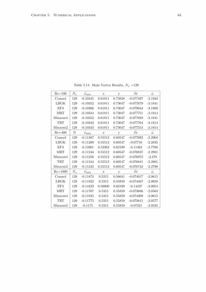
Chapter 5. Numerical Applications 64
Table 5.11: Main Vortex Results, Nx =129
Re=100 Nx ψmin x y δπ ω
Comsol 129 -0.10345 0.61811 0.73828 -0.077497 -3.1943
LBGK 129 -0.10352 0.61811 0.73047 -0.077679 -3.1841
EF3 129 -0.10366 0.61811 0.73047 -0.079044 -3.1869
MRT 129 -0.10344 0.61811 0.73047 -0.077751 -3.1814
Minxent4 129 -0.10352 0.61811 0.73047 -0.077893 -3.1841
TRT 129 -0.10343 0.61811 0.73047 -0.077764 -3.1814
Minxent2 129 -0.10343 0.61811 0.73047 -0.077554 -3.1814
Re=400 N ψmin x y δπ ω
Comsol 129 -0.11387 0.55512 0.60547 -0.077692 -2.2904
LBGK 129 -0.11269 0.55512 0.60547 -0.07716 -2.2835
EF3 129 -0.13361 0.52362 0.62109 -0.11462 -2.7768
MRT 129 -0.11244 0.55512 0.60547 -0.076837 -2.2801
Minxent4 129 -0.11256 0.55512 0.60547 -0.076972 -2.278
TRT 129 -0.11244 0.55512 0.60547 -0.076841 -2.2801
Minxent2 129 -0.11242 0.55512 0.60547 -0.076742 -2.2798
Re=1000 Nx ψmin x y δπ ω
Comsol 129 -0.11874 0.5315 0.56641 -0.074017 -2.0615
LBGK 129 -0.11832 0.5315 0.55859 -0.074487 -2.0658
EF3 129 -0.14423 0.50000 0.62109 -0.14437 -3.0954
MRT 129 -0.11767 0.5315 0.55859 -0.073686 -2.0563
Minxent4 129 -0.11825 0.5315 0.55859 -0.074309 -2.0615
TRT 129 -0.11775 0.5315 0.55859 -0.073815 -2.0577
Minxent2 129 -0.1175 0.5315 0.55859 -0.07321 -2.0535
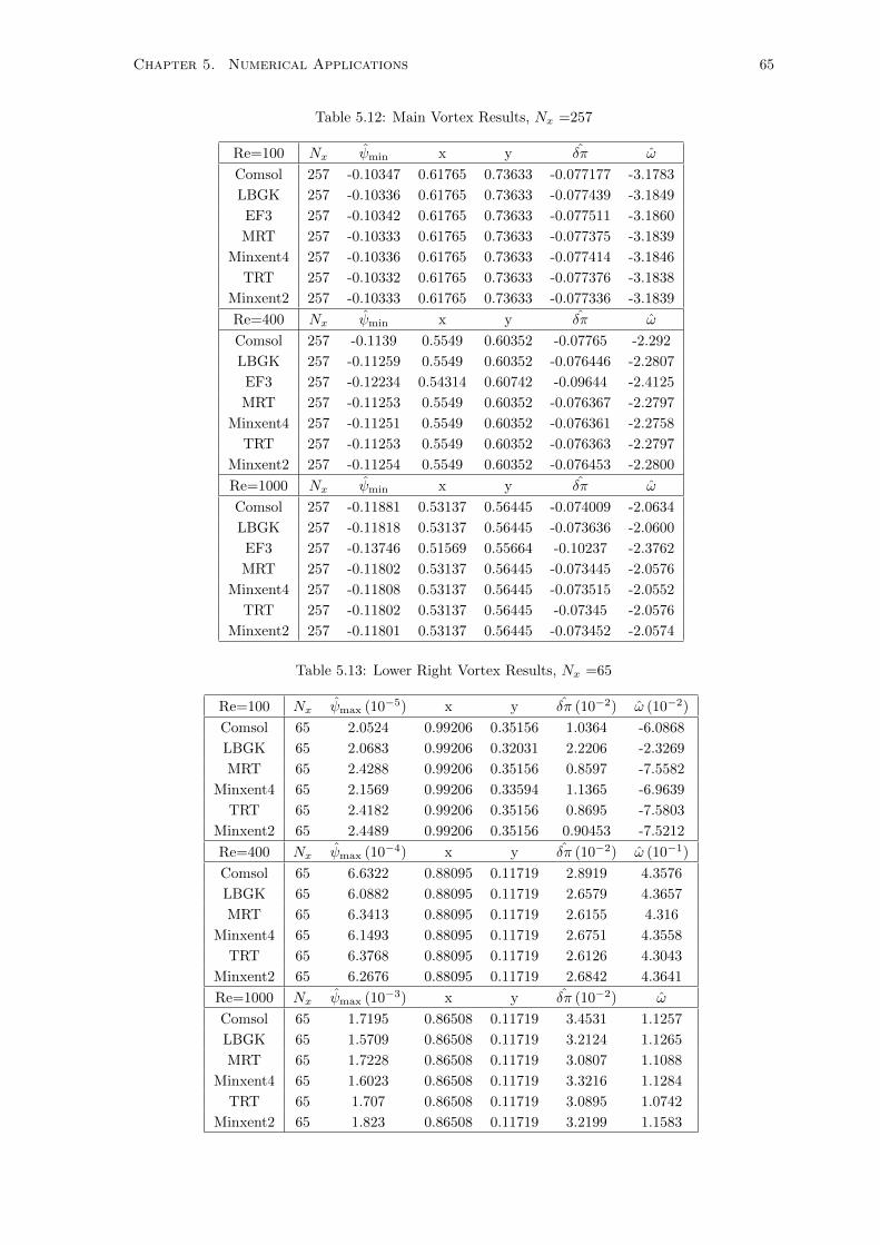
Chapter 5. Numerical Applications 65
Table 5.12: Main Vortex Results, Nx =257
Re=100 Nx ψmin x y δπ ω
Comsol 257 -0.10347 0.61765 0.73633 -0.077177 -3.1783
LBGK 257 -0.10336 0.61765 0.73633 -0.077439 -3.1849
EF3 257 -0.10342 0.61765 0.73633 -0.077511 -3.1860
MRT 257 -0.10333 0.61765 0.73633 -0.077375 -3.1839
Minxent4 257 -0.10336 0.61765 0.73633 -0.077414 -3.1846
TRT 257 -0.10332 0.61765 0.73633 -0.077376 -3.1838
Minxent2 257 -0.10333 0.61765 0.73633 -0.077336 -3.1839
Re=400 Nx ψmin x y δπ ω
Comsol 257 -0.1139 0.5549 0.60352 -0.07765 -2.292
LBGK 257 -0.11259 0.5549 0.60352 -0.076446 -2.2807
EF3 257 -0.12234 0.54314 0.60742 -0.09644 -2.4125
MRT 257 -0.11253 0.5549 0.60352 -0.076367 -2.2797
Minxent4 257 -0.11251 0.5549 0.60352 -0.076361 -2.2758
TRT 257 -0.11253 0.5549 0.60352 -0.076363 -2.2797
Minxent2 257 -0.11254 0.5549 0.60352 -0.076453 -2.2800
Re=1000 Nx ψmin x y δπ ω
Comsol 257 -0.11881 0.53137 0.56445 -0.074009 -2.0634
LBGK 257 -0.11818 0.53137 0.56445 -0.073636 -2.0600
EF3 257 -0.13746 0.51569 0.55664 -0.10237 -2.3762
MRT 257 -0.11802 0.53137 0.56445 -0.073445 -2.0576
Minxent4 257 -0.11808 0.53137 0.56445 -0.073515 -2.0552
TRT 257 -0.11802 0.53137 0.56445 -0.07345 -2.0576
Minxent2 257 -0.11801 0.53137 0.56445 -0.073452 -2.0574
Table 5.13: Lower Right Vortex Results, Nx =65
Re=100 Nx ψmax (10−5) x y δπ (10−2) ω (10−2)
Comsol 65 2.0524 0.99206 0.35156 1.0364 -6.0868
LBGK 65 2.0683 0.99206 0.32031 2.2206 -2.3269
MRT 65 2.4288 0.99206 0.35156 0.8597 -7.5582
Minxent4 65 2.1569 0.99206 0.33594 1.1365 -6.9639
TRT 65 2.4182 0.99206 0.35156 0.8695 -7.5803
Minxent2 65 2.4489 0.99206 0.35156 0.90453 -7.5212
Re=400 Nx ψmax (10−4) x y δπ (10−2) ω (10−1)
Comsol 65 6.6322 0.88095 0.11719 2.8919 4.3576
LBGK 65 6.0882 0.88095 0.11719 2.6579 4.3657
MRT 65 6.3413 0.88095 0.11719 2.6155 4.316
Minxent4 65 6.1493 0.88095 0.11719 2.6751 4.3558
TRT 65 6.3768 0.88095 0.11719 2.6126 4.3043
Minxent2 65 6.2676 0.88095 0.11719 2.6842 4.3641
Re=1000 Nx ψmax (10−3) x y δπ (10−2) ω
Comsol 65 1.7195 0.86508 0.11719 3.4531 1.1257
LBGK 65 1.5709 0.86508 0.11719 3.2124 1.1265
MRT 65 1.7228 0.86508 0.11719 3.0807 1.1088
Minxent4 65 1.6023 0.86508 0.11719 3.3216 1.1284
TRT 65 1.707 0.86508 0.11719 3.0895 1.0742
Minxent2 65 1.823 0.86508 0.11719 3.2199 1.1583

Chapter 5. Numerical Applications 66
Table 5.14: Lower Right Vortex Results, Nx =129
Re=100 Nx ψmax (10−5) x y δπ (10−2) ω (10−2)
Comsol 129 1.2346 0.94094 0.058594 2.03 3.3841
LBGK 129 1.1956 0.94094 0.058594 1.9812 3.3754
EF3 129 1.8127 0.99606 0.37891 0.84294 -4.3343
MRT 129 1.2456 0.94094 0.058594 1.9824 3.3987
Minxent4 129 1.2055 0.94094 0.058594 1.9903 3.3773
TRT 129 1.2458 0.94094 0.058594 1.9813 3.3988
Minxent2 129 1.2454 0.94094 0.058594 2.001 3.3989
Re=400 Nx ψmax(10−4) x y δπ (10−2) ω (10−1)
Comsol 129 6.5059 0.88583 0.12109 2.9161 4.3441
LBGK 129 6.2807 0.88583 0.12109 2.7841 4.3278
EF3 129 15.476 0.8937 0.17578 3.1705 5.4661
MRT 129 6.3231 0.88583 0.12109 2.7714 4.316
Minxent4 129 6.2799 0.88583 0.12109 2.7767 4.3226
TRT 129 6.3236 0.88583 0.12109 2.7714 4.316
Minxent2 129 6.3171 0.88583 0.12109 2.7768 4.3177
Re=1000 Nx ψmax (10−3) x y δπ (10−2) ω
Comsol 129 1.7229 0.8622 0.11328 3.5042 1.1407
LBGK 129 1.6922 0.8622 0.11328 3.4109 1.1415
EF3 129 4.0688 0.75197 0.15234 5.062 1.0785
MRT 129 1.7113 0.8622 0.11328 3.3699 1.1317
Minxent4 129 1.693 0.8622 0.11328 3.4136 1.1409
TRT 129 1.7124 0.8622 0.11328 3.371 1.1308
Minxent2 129 1.7167 0.8622 0.11328 3.3927 1.1386

Chapter 5. Numerical Applications 67
Table 5.15: Lower Right Vortex Results, Nx =257
Re=100 Nx ψmax (10−5) x y δπ (10−2) ω (10−2)
Comsol 257 1.2457 0.94314 0.060547 2.0433 3.4253
LBGK 257 1.2455 0.94314 0.060547 2.0196 3.3532
EF3 257 1.2483 0.94314 0.060547 2.0223 3.3518
MRT 257 1.2539 0.94314 0.060547 2.0184 3.3586
Minxent4 257 1.2477 0.94314 0.060547 2.0213 3.3539
TRT 257 1.2539 0.94314 0.060547 2.0183 3.3586
Minxent2 257 1.254 0.94314 0.060547 2.0227 3.3585
Re=400 Nx ψmax (10−4) x y δπ (10−2) ω (10−1)
Comsol 257 6.4492 0.88431 0.12305 2.935 4.7086
LBGK 257 6.303 0.88431 0.12305 2.8272 4.5192
EF3 257 12.536 0.99804 0.46289 0.80144 -0.72403
MRT 257 6.2994 0.88431 0.12305 2.8279 4.5172
Minxent4 257 6.2862 0.88431 0.12305 2.8188 4.5149
TRT 257 6.2993 0.88431 0.12305 2.8281 4.5172
Minxent2 257 6.3046 0.88431 0.12305 2.8189 4.5169
Re=1000 Nx ψmax (10−3) x y δπ (10−2) ω
Comsol 257 1.7192 0.86471 0.11133 3.5281 1.0996
LBGK 257 1.7092 0.86471 0.11133 3.4585 1.0812
EF3 257 1.785 0.86471 0.12695 4.3053 1.2018
MRT 257 1.7125 0.86471 0.11133 3.447 1.0784
Minxent4 257 1.7071 0.86471 0.11133 3.4503 1.0801
TRT 257 1.7126 0.86471 0.11133 3.4468 1.0784
Minxent2 257 1.7128 0.86471 0.11133 3.4446 1.0786
Table 5.16: Lower Left Vortex Results, Nx=65
Re=100 Nx ψmax (10−6) x y δπ (10−2) ω (10−2)
Comsol 65 1.0982 0.039683 0.023438 1.6134 0.86636
LBGK 65 0.09497 0.039683 0.023438 1.346 0.93154
MRT 65 1.1721 0.039683 0.023438 1.4454 0.91345
Minxent4 65 0.11672 0.02381 0.023438 1.4741 0.28755
TRT 65 1.1531 0.039683 0.023438 1.4411 0.90138
Minxent2 65 1.2201 0.039683 0.023438 1.5134 0.93364
Re=400 Nx ψmax (10−5) x y δπ (10−2) ω (10−2)
Comsol 65 1.0932 0.055556 0.039063 3.5813 4.7404
LBGK 65 0.74957 0.055556 0.039063 3.3114 4.5015
MRT 65 1.LBGK4 0.055556 0.039063 3.2633 4.5903
Minxent4 65 0.83092 0.055556 0.039063 3.3339 4.5133
TRT 65 1.1083 0.055556 0.039063 3.2676 4.5883
Minxent2 65 1.0901 0.055556 0.039063 3.3058 4.6056
Re=1000 Nx ψmax (10−4) x y δπ (10−2) ω (10−1)
Comsol 65 2.0277 0.087302 0.070313 4.4541 3.1701
LBGK 65 1.8388 0.087302 0.070313 4.1189 3.0663
MRT 65 1.9182 0.087302 0.070313 4.0079 3.0087
Minxent4 65 1.8264 0.087302 0.070313 4.2898 3.0681
TRT 65 1.9459 0.087302 0.070313 4.0818 3.0275
Minxent2 65 1.939 0.087302 0.070313 4.0693 2.9862

Chapter 5. Numerical Applications 68
Table 5.17: Lower Left Vortex Results, Nx =129
Re=100 Nx ψmax(10−6) x y δπ(10−2) ω(10−2)
Comsol 129 1.4813 0.035433 0.035156 1.6337 1.6403
LBGK 129 1.3208 0.035433 0.035156 1.5642 1.5854
EF3 129 1.3425 0.035433 0.035156 1.5279 1.586
MRT 129 1.6117 0.035433 0.035156 1.5639 1.6115
Minxent4 129 1.3759 0.035433 0.035156 1.5731 1.5919
TRT 129 1.6123 0.035433 0.035156 1.5628 1.6115
Minxent2 129 1.6135 0.035433 0.035156 1.5826 1.6121
Re=400 Nx ψmax(10−5) x y δπ(10−2) ω(10−2)
Comsol 129 1.2735 0.051181 0.042969 3.5971 5.0593
LBGK 129 1.2243 0.051181 0.042969 3.4392 4.8987
EF3 129 9.9055 0.35039 0.011719 3.3262 97.345
MRT 129 1.2871 0.051181 0.042969 3.4249 4.9082
Minxent4 129 1.2423 0.051181 0.042969 3.4334 4.9066
TRT 129 1.2873 0.051181 0.042969 3.4249 4.9083
Minxent2 129 1.2857 0.051181 0.042969 3.4296 4.907
Re=1000 Nx ψmax(10−4) x y δπ(10−2) ω(10−1)
Comsol 129 2.183 0.082677 0.074219 4.4655 3.2451
LBGK 129 2.1756 0.082677 0.074219 4.3529 3.1771
EF3 129 22.271 0.16142 0.14453 5.009 7.7776
MRT 129 2.1942 0.082677 0.074219 4.3132 3.1633
Minxent4 129 2.1835 0.082677 0.074219 4.3571 3.1804
TRT 129 2.1981 0.082677 0.074219 4.3182 3.1662
Minxent2 129 2.1887 0.082677 0.074219 4.3234 3.158

Chapter 5. Numerical Applications 69
Table 5.18: Lower Left Vortex Results, Nx =257
Re=100 Nx ψmax(10−6) x y δπ(10−2) ω(10−2)
Comsol 257 1.6489 0.033333 0.033203 1.6384 1.3439
LBGK 257 1.6893 0.033333 0.033203 1.6029 1.3356
EF3 257 1.6903 0.033333 0.033203 1.6061 1.3363
MRT 257 1.7358 0.033333 0.033203 1.6012 1.3394
Minxent4 257 1.7009 0.033333 0.033203 1.6046 1.3366
TRT 257 1.7358 0.033333 0.033203 1.6011 1.3394
Minxent2 257 1.7356 0.033333 0.033203 1.6056 1.3394
Re=400 Nx ψmax(10−5) x y δπ(10−2) ω(10−2)
Comsol 257 1.3374 0.052941 0.044922 3.6042 5.6698
LBGK 257 1.3307 0.052941 0.044922 3.4853 5.5808
EF3 257 2.0191 0.052941 0.052734 3.8607 8.3503
MRT 257 1.3405 0.052941 0.044922 3.4778 5.5812
Minxent4 257 1.3331 0.052941 0.044922 3.4734 5.5837
TRT 257 1.3406 0.052941 0.044922 3.478 5.5813
Minxent2 257 1.3412 0.052941 0.044922 3.4722 5.5813
Re=1000 Nx ψmax(10−4) x y δπ(10−2) ω(10−1)
Comsol 257 2.2514 0.084314 0.076172 4.4704 3.5089
LBGK 257 2.2549 0.084314 0.076172 4.3907 3.4114
EF3 257 2.9686 0.088235 0.076172 5.5588 4.2134
MRT 257 2.2569 0.084314 0.076172 4.3797 3.4068
Minxent4 257 2.255 0.084314 0.076172 4.382 3.4119
TRT 257 2.2571 0.084314 0.076172 4.3797 3.4069
Minxent2 257 2.2562 0.084314 0.076172 4.3764 3.406

Chapter 6
Conclusions
6.1 Conclusions
We began this thesis by describing the traditional interpretations of the single relaxation time Lat-
tice Boltzmann Method; as a generalization of the Lattice Gas Automata or as a discretization of
the Boltzmann Equation. In the pursuit of increasing the stability of the LBM, some researchers
attempted to equip the LBM with an H-Theorem. The H-Theorem would provide an equilibrium
that is the minimizer of some entropy function and would also act as an attractor. It is hypothesized
that an equilibrium with these features would help stabilize the method. The most popular of these
methods is called the Entropic Lattice Boltzmann Method (ELBM).
The ELBM has been criticized by other researchers who believed that the most promising and
practical route to stabilization was by using multiple relaxation times. This has led to somewhat of
a split in the LBM community; those who embrace entropic methods such as ELBM and entropic
limiters, and those who prefer multiple relaxation times.
We however believe that these two seemingly dissimilar approaches are specific implementations of
our unified interpretation of LBM. We proposed that the LBM is a split-time scheme that implements
the principle of Minimum Discrimination INformation (MinxEnt). Indeed we show that the entropic
methods and relaxation time methods are specific approximations of MinxEnt-LBM. In this way we
unify the entropic and relaxation time schemes.
Because the entropic and relaxation time schemes are approximations of MinxEnt-LBM, we
expect that MinxEnt-LBM should have superior stability characteristics. This indeed was shown
in numerical simulations carried out here. The only scheme that performed superior to MinxEnt-
LBM was the entropy limiting scheme of the LBM based on Ehrenfest Steps (EF-LBM). However,
lid driven cavity flow simulations showed that without tuning the parameters involved in EF-LBM
schemes they suffered from a degradation of accuracy. We can conclude that, of the LBM schemes
tested, MinxEnt-LBM had the best combination of stability and accuracy.
An important practical consideration should also be noted here. EF-LBM and MRT-LBM require
specification of parameters which need to be tuned and optimal values are not known a priori. This
is not the case for the MinxEnt-LBM.
Finally, the development of the MinxEnt-LBM scheme was based on constraints and an entropy
function only, and did not use the Navier-Stokes equations to obtain values for its parameters. This
cannot be said about the other LBM schemes described here. This means that the MinxEnt-LBM is
much more suited to be applied to non-fluid systems or systems in which the governing macroscopic
equations are unknown.
70

Chapter 6. Conclusions 71
6.2 Future Work
The MinxEnt-LBM described here used a single step Newton-Raphson method to perform the min-
imizations. It is hypothesized here that instabilities occur in the LBM due to inaccuracies in these
minimizations. This suggests a route for enhancing stability; use more sophisticated, robust and
accurate methods than Newton-Raphson to perform the minimization.
Also, due to the aforementioned general nature of the MinxEnt-LBM, work that uses MinxEnt-
LBM to simulate non-fluid related physical systems may be explored. In fact, nothing in the devel-
opment of the MinxEnt-LBM scheme suggested that it could only be applied to mass transport type
problems. This would make MinxEnt-LBM a promising method to explore systems which have no
pre-defined governing equations. One possible application may be to simulate a system at the mi-
croscopic level (using other methods such as Molecular Dynamics simulations, or Density Functional
Theory) to obtain constraints inherent (and non-obvious) to the system. These constraints could
then be used in the MinxEnt-LBM scheme to simulate the mesoscopic or macroscopic evolution of
the system. In this way, the macroscopic governing equations would be an emergent property of the
method, and not a crucial ingredient.
Our novel interpretation of the Lattice Boltzmann Method not only improves the stability and
accuracy of the current implementations of the LBM, but also provides a unifying framework on
which to base them on. This framework opens a large number of different possibilities for future
improvements to the Lattice Boltzmann Method and a much wider range of possible applications.

Appendices
72

Appendix A
Probability and Mass Expectation
Distributions
Consider a classical system, of a large number, N , of identical particles of mass m in D dimensions.
Rather than track the particles individually we treat the position and velocity of each particle as
random variables.
X(t) = Xj(t) | j = 1 . . . N,
V (t) = Vj(t) | j = 1 . . . N,
where Xj and Vj are random variables describing the jth particle’s position and velocity respectively.
We define a “microscopic state,” Γ, to be a vector of specific realizations of the random positions
and velocities of the particles. That is,
Γ(t) = 〈X1(t) = x1, . . . ,XN (t) = xN ,V1(t) = v1, . . .VN (t) = vN 〉.
Imagine that we would like to predict the value of a macroscopic observable quantity that is
a function of the positions and velocities of all of the particles in the system. Call this function
G(Γ(t)). Rather than measure actual values for G, laboratory devices usually measure time averages
of G. That is, devices measure Gobs which is given by,
Gobs(t) =1
∆t
∫ t+∆t
t
G(Γ(s)) ds.
This suggests that following the precise location of all the particles at all times may in fact give us
more information than we could actually use. With this in mind we wish to find a way to track these
averaged quantities instead.
Given a specific position x and velocity v we denote the joint probability of finding a particle
with velocity v and at position x at time t as,
pjoint(x,v, t) ≡ P
N⋃j=1
(Xj(t) = x
⋂Vj(t) = v
) , (A.1)
where P (Y ) denotes the probability of event Y occurring. We also denote the conditional probability
73

Appendix A. Probability and Mass Expectation Distributions 74
of finding a particle with velocity v given that it is located at position x as,
p(x,v, t) ≡ P
N⋃j=1
(Vj(t) = v | Xj(t) = x)
.Finally the marginal probability of finding a particle at position x at time t (regardless of its velocity)
as,
pmarg(x, t) ≡ P
N⋃j=1
(Xj(t) = x)
.We now define the the mass expectation density, f , to be,
f(x,v, t) := Nmpjoint(x,v, t), (A.2)
and note that f has the following properties,∫f(x,v, t)dv = ρ(x, t) = Nmpmarg(x, t),∫
f(x,v, t) dvdx = Nm,
where ρ(x, t) is the mass density at position x at time t.
The relationship between f and p can be found by using the definition of conditional probability.
For events A and B, the conditional probability is defined by,
P (A|B) =P (A ∩B)
P (B),
which for us becomes,
p(x,v, t) =pjoint(x,v, t)
pmarg(x, t)
And so for our system,
f(x,v, t) = Nmpjoint(x,v, t)
= Nmp(x,v, t)pmarg(x, t),
= p(x,v, t)
∫f(x,v, t) dv,
= p(x,v, t)ρ(x, t),
and thus, if the mass density is non-zero then,
p(x,v, t) =f(x,v, t)
ρ(x, t). (A.3)
Note that for all positions and times, p is a probability distribution with respect to v,∫p(x,v, t) dv = 1,

Appendix A. Probability and Mass Expectation Distributions 75
Consider a vector of k macroscopic quantities
M(t) := 〈M1(X(t),V(t)), ..,Mk(X(t),V(t))〉,
such as density, mean velocity, temperature, etc. Further, letM(t) denote a vector of k realizations
of these macroscopic quantities at a given time t,
M(t) := 〈M1, ...,Mk〉.
In this case we say that at time t a system is in the “macroscopic state,” M(t).
A system in a given macroscopic state could be in any of a large number of different microscopic
states. The set of all microscopic states that share the same macroscopic state is called the ensemble;
denoted E ,
E(M(t)) := Γ(t) |M(t) =M(t)
Now, suppose that at a given time t, and that the system is in macroscopic state,M(t). We can
define the following quantities,
P (Γ(t)) :=probability that the system is in microscopic state Γ(t)
P [Γ(t)|M(t)] :=probability of the system being in microscopic state Γ(t)
given it’s in macroscopic state M(t)
P [(x,v, t) ∩ Γ(t)] :=probability of a particle being at position x with velocity v
and that the system is in microscopic state Γ(t)
P [Γ | (x,v, t)] := probability that the system is in microscopic state Γ(t)
given that there is a particle at position x with velocity v
Using these definitions and the axioms of probability we can calculate the ensemble average, 〈G〉, of
observable G. Let dΓ = dx1...dxNdv1...dvN be the differential change in the microscopic state then
we have,
〈G〉(t) =
∫Γ∈E
P (Γ)G(Γ) dΓ
=
∫Γ∈E
∫∫P [(x′,v′, t) ∩ Γ] G(Γ) dx′ dv′ dΓ
=
∫Γ∈E
∫∫pjoint(x
′,v′, t)P [Γ|(x′,v′, t)] G(Γ) dx′ dv′ dΓ
=
∫∫pjoint(x
′,v′, t)
∫Γ∈E
P [Γ|(x′,v′, t)] G(Γ) dx′ dv′ dΓ
=
∫∫pjoint(x
′,v′, t) g(x′,v′, t) dx′ dv′ (A.4)
where we have defined
g(x′,v′, t) ≡∫
Γ∈EP (Γ|(x′,v′, t))G(Γ) dΓ. (A.5)
One can think of g(x,v, t) as representing the expectation value of the observable, G, given that
there is a particle located at position x, with velocity v, at time t.
Assuming the ergodic hypothesis holds, we can equate the ensemble average and the time average

Appendix A. Probability and Mass Expectation Distributions 76
and so,
Gobs(t) = 〈G〉(t) =
∫∫pjoint(x
′,v′, t) g(x′,v′, t) dx′ dv′.
For example, to evaluate the observed macroscopic density, ρ, at position x at time t we would
use g(x′,v′, t) = Nmδ(x′ − x) in (A.4),
ρ(x, t) =
∫∫Nmpjoint(x
′,v′, t) δ(x′ − x) dx′ dv′ (A.6)
For the macroscopic momentum, ρu, at position x at time t at position x at time t we would use
g(x′,v′, t) = Nmv′ δ(x′ − x),
ρ(x, t)u(x, t) =
∫∫v′Nmpjoint(x
′,v′, t) δ(x′ − x) dx′ dv′ (A.7)
Recalling the mass expectation density, (A.2), we can write,
ρ(x, t) =
∫∫f(x′,v′, t) δ(x′ − x) dx′ dv′
=
∫f(x,v′, t) dv′
ρ(x, t)u(x, t) =
∫∫f(x′,v′, t)v′ δ(x′ − x) dx′ dv′
=
∫f(x,v′, t) v′ dv′
It is still an area of active research as to the conditions under which the ergodic hypothesis holds.
However, we will assume that it holds.

Appendix B
D2Q9 Fluid Constraint
B.1 Isotropic Newtonain Fluids
From continuum mechanics we know that any continuum that obeys conservation of mass follows
the Cauchy momentum equation,
ρdu
dt= ∇ · σ + ρg
where ρ is the mass density, u is the macroscopic velocity, σ is the Cauchy stress tensor and g is a
body force. In kinetic theory σ is related to the mass expectation distribution by,
σjk(x, t) =
∫f(x,v, t)(v − u)j(v − u)k dv
=
∫f(x,v, t)vjvk dv − ρujuk
For an isotropic Newtonian fluid the stress tensor is related to the strain-rate tensor by,
σjk = −πδjk + 2µεjk (B.1)
where π is the hydrostatic pressure, µ is the kinematic viscosity and ε is the strain-rate tensor,
εjk =1
2
[∂uj∂xk
+∂uk∂xj
].
In what follows we will derive the constraints that need to be applied to the collision step to
ensure (B.1) holds and thus allow an LBM simulation to simulate an isotropic Newtonian fluid.
B.2 D2Q9 LBM Configuration
Recall the two dimensional, 9 velocity LBM. The velocity set is given in Table B.1.
Table B.1: D2Q9 Velocity Scheme: c =√
3RT
i 1 2 3 4 5 6 7 8 9
vi (c,0) (0,c) (-c,0) (0,-c) (c,c) (-c,c) (-c,-c) (c,-c) (0,0)
Wi19
19
19
19
136
136
136
136
49
The streaming step and the discrete polynomial equilibrium is given in equations (B.2) and (B.3)
77

Appendix B. D2Q9 Fluid Constraint 78
respectively,
fi(x + viδt, t+ δt) = fposti (x, t), (B.2)
f eqi = ρWi
1− 3|u|2
2c2+
3vi · uc2
+9(vi · u)2
2c4
. (B.3)
B.3 D2Q9 Tensor Identities
From the expression for the equilibrium distribution (B.3), one can easily show that in D2Q9 we
have the following identities [11],
9∑i=1
f eqi = ρ, (B.4)
9∑i=1
f eqi vi,j = ρuj , (B.5)
9∑i=1
f eqi vi,jvi,k =
1
3c2ρδjk + ρujuk, (B.6)
9∑i=1
f eqi vi,jvi,kvi,l =
1
3c2ρ (δjkul + δkluj + δjluk) , (B.7)
B.4 Chapman-Enskog Expansion
We will perform a procedure based on the one outlined in the appendix of [11] (commonly known as
Chapman-Enskog analysis). For brevity, we introduce the expansion parameter ε = δt and assume
that ε << 1.
Performing a Taylor expansion,
fi(x + viδt, t+ δt) =
∞∑n=0
εn
n!Dnfpre
i (B.8)
where we define the multi-scale expansions,
D := D0 + εD1 +O(ε2),
D0 :=∂
∂t0+
2∑k=1
vi,k∂
∂xk,
D1 :=∂
∂t1∂
∂t=
∂
∂t0+ ε
∂
∂t1+O(ε2).
We also expand the pre-collision distribution,
fprei = f eq
i + εf1i +O(ε2). (B.9)

Appendix B. D2Q9 Fluid Constraint 79
We will also find it useful to define,
Π0jk :=
9∑i=1
f eqi vi,jvi,k (B.10)
Π1jk :=
9∑i=1
f1i vi,jvi,k (B.11)
With these expansions in hand, we now show that choosing the equilibrium as (B.3) and ensuring
the collision has 3 important properties has the consequence that we recover the LBM version of the
Cauchy momentum equation and satisfy (B.1).
B.5 Consequences of Equilibrium and Collision Constraints
Theorem B.5.1. If the equilibrium distribution is given as in (B.3), and the collision step satisfies
the following three properties,
1.∑9i=1 fpost
i =∑9i=1 fpre
i
2.∑9i=1 fpost
i vi,j =∑9i=1 fpre
i vi,j
3.∑9i=1D0f
eqi vi,jvi,k = − 1
τ
∑9i=1 f1
i vi,jvi,k
then the D2Q9 version of LBM will simulate the continuity equation and modified Cauchy momentum
equation,
∂ρ
∂t+∇ · (ρu) = 0
ρdu
dt= ∇ · σLBM
where,
σLBM = −c2
3ρ+ 2µεjk,
and
µ = ερc2
3
(2τ − 1
2
),
up to O(ε2) and O(u3)
Proof. Before beginning we make note of the following fact,
ρ =
9∑i=1
fprei
=
9∑i=1
f eqi + εf1
i +O(ε2)
= ρ+ εf1i +O(ε2)
and thus,
9∑i=1
f1i = O(ε). (B.12)

Appendix B. D2Q9 Fluid Constraint 80
Similarly,
ρu =
9∑i=1
fprei vi
=
9∑i=1
f eqi vi + εf1
i vi +O(ε2)
= ρu + +εf1i vi +O(ε2)
And so,
9∑i=1
f1i vi = O(ε). (B.13)
Starting with the local conservation of mass property of the collision step and making use of the
streaming step (B.2) and expansion (B.9) we have,
9∑i=1
fposti =
9∑i=1
fprei ,
9∑i=1
fi(x + viδt, t+ δt) =
9∑i=1
fprei ,
=
9∑i=1
f eqi + εf1
i +O(ε2)
and thus from the Taylor expansion (B.8),
9∑i=1
∞∑n=0
εn
n!Dnfpre
i =
9∑i=1
f eqi + εf1
i +O(ε2).
Equating orders of ε we obtain,
O(ε) :9∑i=1
D0feqi = 0 (B.14)
O(ε2) :
9∑i=1
D0f1i +
1
2D2
0f eqi +D1f
eqi = O(ε2) (B.15)
Likewise from the local conservation of momentum property of the collision step we get,
9∑i=1
∞∑n=0
εn
n!Dnfpre
i vi =
9∑i=1
f eqi vi + εf1
i vi +O(ε2)
Again equating orders of ε,
O(ε) :
9∑i=1
D0feqi vi = 0 (B.16)
O(ε2) :
9∑i=1
D0f1i vi +
1
2D2
0f eqi vi +D1f
eqi vi = O(ε2) (B.17)

Appendix B. D2Q9 Fluid Constraint 81
Note that,
9∑i=1
D20f eqi =
9∑i=1
D0D0feqi
=
9∑i=1
(∂
∂t0+
2∑k=1
vi,k∂
∂xk
)D0f
eqi
=∂
∂t0
9∑i=1
D0feqi +
2∑k=1
∂
∂xk
9∑i=1
D0feqi vi,k.
Using (B.14) and (B.16) we have,
9∑i=1
D20f eqi = 0. (B.18)
Similarly we can use (B.16) and the assumed third property of the collision step to show,
9∑i=1
D20f eqi vi,j = −1
τ
9∑i=1
D0f1i vi,j . (B.19)
Equations (B.18) and (B.19) allow (B.14) and (B.15) to become,
O(ε) :∂ρ
∂t0+∇ · (ρu) = 0, (B.20)
O(ε2) :∂ρ
∂t1= O(ε2), (B.21)
as well as (B.16) and (B.17) to become,
O(ε) :∂ρu
∂t0+∇ ·Π0 = 0 (B.22)
O(ε2) :∂ρu
∂t1+
(2τ − 1
2τ
)∇ ·Π1 = O(ε2) (B.23)
Taking (B.20) + ε(B.21),
∂ρ
∂t+∇ · (ρu) = O(ε3), (B.24)
and (B.22) + ε(B.23),
∂ρu
∂t+∇ ·
[Π0 + ε
(2τ − 1
2τ
)Π1
]= O(ε3). (B.25)
Recalling the definitions (B.10) and (B.11) we can use the identities from (B.4)-(B.7) to rewrite
(B.25) as,
ρdu
dt= ∇ · σLBM +O(ε2),
where ddt is the material derivative,
d
dt=
∂
∂t+ u · ∇,
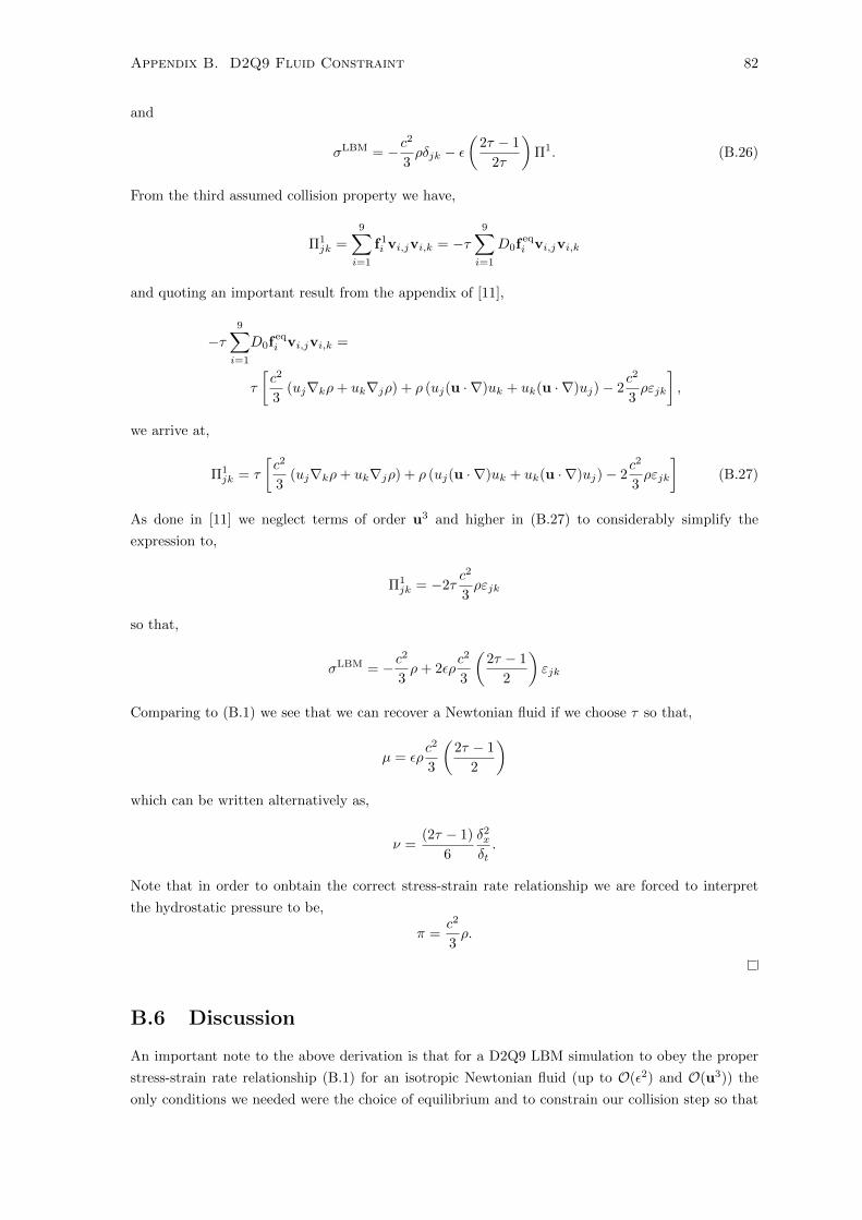
Appendix B. D2Q9 Fluid Constraint 82
and
σLBM = −c2
3ρδjk − ε
(2τ − 1
2τ
)Π1. (B.26)
From the third assumed collision property we have,
Π1jk =
9∑i=1
f1i vi,jvi,k = −τ
9∑i=1
D0feqi vi,jvi,k
and quoting an important result from the appendix of [11],
−τ9∑i=1
D0feqi vi,jvi,k =
τ
[c2
3(uj∇kρ+ uk∇jρ) + ρ (uj(u · ∇)uk + uk(u · ∇)uj)− 2
c2
3ρεjk
],
we arrive at,
Π1jk = τ
[c2
3(uj∇kρ+ uk∇jρ) + ρ (uj(u · ∇)uk + uk(u · ∇)uj)− 2
c2
3ρεjk
](B.27)
As done in [11] we neglect terms of order u3 and higher in (B.27) to considerably simplify the
expression to,
Π1jk = −2τ
c2
3ρεjk
so that,
σLBM = −c2
3ρ+ 2ερ
c2
3
(2τ − 1
2
)εjk
Comparing to (B.1) we see that we can recover a Newtonian fluid if we choose τ so that,
µ = ερc2
3
(2τ − 1
2
)which can be written alternatively as,
ν =(2τ − 1)
6
δ2x
δt.
Note that in order to onbtain the correct stress-strain rate relationship we are forced to interpret
the hydrostatic pressure to be,
π =c2
3ρ.
B.6 Discussion
An important note to the above derivation is that for a D2Q9 LBM simulation to obey the proper
stress-strain rate relationship (B.1) for an isotropic Newtonian fluid (up to O(ε2) and O(u3)) the
only conditions we needed were the choice of equilibrium and to constrain our collision step so that

Appendix B. D2Q9 Fluid Constraint 83
it has the aforementioned properties,
9∑i=1
fposti =
9∑i=1
fprei (B.28)
9∑i=1
fposti vi,j =
9∑i=1
fprei vi,j (B.29)
9∑i=1
D0feqi vi,jvi,k = −1
τ
9∑i=1
f1i vi,jvi,k (B.30)
Of course way to implement the constraint (B.30) is the usual MRT-LBM expression,
9∑i=1
fposti vi,jvi,k =
9∑i=1
fprei vi,jvi,k +
1
τ(f eqi − fpre
i ) vi,jvi,k, (B.31)
which in the moment description of §4.3.4 was written as,
Mpostk = Mpre
k +1
τ(Meq
k −Mprek ) , k ∈ 8, 9.
This realization has an interesting consequence; one does not need a collision step as restrictive as
the SRT-LBM expression,9∑i=1
fposti =
9∑i=1
fprei +
1
τ(f eqi − fpre
i ) ,
in order to simulate a Newtonian fluid. All that is required is that (B.28)-(B.30) are satisfied. In fact,
we can take this interpretation further and state that it is not even necessary for the collision step
to assume the usual MRT-LBM form (B.31). In principle, any constraints on the collision step will
suffice provided they have properties (B.28)-(B.30). This opens the door to new ways of constraining
the collision step yet still ensuring the proper physics.

Bibliography
[1] Haihu Liu et al. “Multiphase lattice Boltzmann simulations for porous media applications – a
review”. In: (Apr. 2014), p. 51. arXiv: 1404.7523.
[2] Guy R McNamara and Gianluigi Zanetti. “Use of the Boltzmann equation to simulate lattice-
gas automata”. In: Physical Review Letters 61.20 (1988), p. 2332.
[3] FJ J Higuera, S Succi, and R Benzi. “Lattice gas dynamics with enhanced collisions”. In: EPL
(Europhysics Letters) 345.4 (June 1989), pp. 345–349. doi: 10.1209/0295-5075/9/4/008.
[4] F J Higuera and J Jimenez. “Boltzmann approach to lattice gas simulations”. In: EPL (Euro-
physics Letters) 9.7 (1989), p. 663.
[5] Shiyi Chen et al. “Lattice Boltzmann model for simulation of magnetohydrodynamics”. In:
Physical Review Letters 67.27 (1991), p. 3776.
[6] Roberto Benzi, Sauro Succi, and Massimo Vergassola. “The lattice Boltzmann equation: theory
and applications”. In: Physics Reports 222.3 (1992), pp. 145–197.
[7] Hudong Chen, Shiyi Chen, and William H Matthaeus. “Recovery of the Navier-Stokes equations
using a lattice-gas Boltzmann method”. In: Physical Review A 45.8 (1992), R5339.
[8] YH Qian, D D’Humieres, and P Lallemand. “Lattice BGK models for Navier-Stokes equation”.
In: EPL (Europhysics Letters) 479 (1992).
[9] J.-P. Rivet and J. P. Boon. Lattice Gas Hydrodynamics. Cambridge University Press, 2005,
p. 312.
[10] Bastien Chopard and Michel Droz. Cellular Automata Modeling of Physical Systems. Cam-
bridge University Press, 2005, p. 341.
[11] Xiaoyi He and LS Luo. “A priori derivation of the lattice Boltzmann equation”. In: Physical
Review E 55.6 (1997), pp. 6333–6336.
[12] Xiaoyi He and Li-Shi Luo. “Lattice Boltzmann Model for the Incompressible NavierStokes
Equation”. In: Journal of Statistical Physics 88.3/4 (Aug. 1997), pp. 927–944. doi: 10.1023/B:
JOSS.0000015179.12689.e4.
[13] Xiaoyi He and Li-Shi Luo. “Theory of the lattice Boltzmann method: From the Boltzmann
equation to the lattice Boltzmann equation”. In: Physical Review E 56.6 (Dec. 1997), pp. 6811–
6817. doi: 10.1103/PhysRevE.56.6811.
[14] M. K. Banda, W. A. Yong, and A. Klar. “A Stability Notion for Lattice Boltzmann Equations”.
In: SIAM Journal on Scientific Computing 27.6 (Jan. 2006), pp. 2098–2111. doi: 10.1137/
040606211.
[15] JD Sterling and S Chen. “Stability analysis of lattice Boltzmann methods”. In: Journal of
Computational Physics 206.123 (1996), pp. 196–206.
84

BIBLIOGRAPHY 85
[16] Yanbing Li et al. “Numerical study of flow past an impulsively started cylinder by the lattice-
Boltzmann method”. In: Journal of Fluid Mechanics 519 (2004), pp. 273–300.
[17] F. Tosi et al. “Numerical stability of Entropic versus positivity-enforcing Lattice Boltzmann
schemes”. In: Mathematics and Computers in Simulation 72.2-6 (Sept. 2006), pp. 227–231.
doi: 10.1016/j.matcom.2006.05.007.
[18] B. M. BM Boghosian et al. “Entropic lattice Boltzmann methods”. In: Proceedings of the Royal
Society A: Mathematical, Physical and Engineering Sciences 457.2007 (Mar. 2001), pp. 717–
766. doi: 10.1098/rspa.2000.0689.
[19] Ludwig Boltzmann. “Further Studies on the Thermal Equilibrium of Gas Molecules”. In: The
Kinetic Theory of Gases. Vol. Volume 1. History of Modern Physical Sciences. Imperial College
Press, July 2003, pp. 262–349. doi: doi:10.1142/9781848161337\_0015.
[20] Hudong Chen and Chris Teixeira. “H-theorem and origins of instability in thermal lattice
Boltzmann models”. In: Computer Physics Communications 129.1-3 (July 2000), pp. 21–31.
doi: 10.1016/S0010-4655(00)00089-8.
[21] Sauro Succi, Iliya Karlin, and Hudong Chen. “Colloquium: Role of the H theorem in lat-
tice Boltzmann hydrodynamic simulations”. In: Reviews of Modern Physics 74.4 (Nov. 2002),
pp. 1203–1220. doi: 10.1103/RevModPhys.74.1203.
[22] Santosh Ansumali and Iliya Karlin. “Stabilization of the lattice Boltzmann method by the
H theorem:A numerical test”. In: Physical Review E 62.6 (Dec. 2000), pp. 7999–8003. doi:
10.1103/PhysRevE.62.7999.
[23] Bruce Boghosian et al. “Galilean-invariant lattice-Boltzmann models with H theorem”. In:
Physical Review E 68.2 (Aug. 2003), p. 025103. doi: 10.1103/PhysRevE.68.025103. arXiv:
0211093v1 [arXiv:cond-mat].
[24] Sauro Succi. The Lattice Boltzmann Equation: For Fluid Dynamics and Beyond. Oxford Uni-
versity Press, 2001, p. 288.
[25] IV Iliya Karlin and S. Succi. “Equilibria for discrete kinetic equations”. In: Physical Review E
58.4 (Oct. 1998), pp. 4053–4056. doi: 10.1103/PhysRevE.58.R4053.
[26] Iliya Karlin et al. “Maximum Entropy Principle for Lattice Kinetic Equations”. In: Physical
Review Letters 81.1 (July 1998), pp. 6–9. doi: 10.1103/PhysRevLett.81.6.
[27] A Renda et al. “Thermohydrodynamic lattice BGK schemes with non-perturbative equilibria”.
en. In: Europhysics Letters (EPL) 41.3 (Feb. 1998), pp. 279–284. doi: 10.1209/epl/i1998-
00143-x.
[28] IV Karlin, A Ferrante, and HC Ottinger. “Perfect entropy functions of the lattice Boltzmann
method”. In: EPL (Europhysics Letters) 47.July (1999), pp. 182–188.
[29] Alexander J. Wagner. “An H-Theorem for the Lattice Boltzmann Approach to Hydrodynam-
ics”. In: EPL (Europhysics Letters) 29.April 1995 (Aug. 1998), p. 6. doi: 10.1209/epl/i1998-
00448-8. arXiv: 9808052 [cond-mat].
[30] Bruce M Boghosian, Peter Love, and Jeffrey Yepez. “Entropic lattice Boltzmann model for
Burgers’s equation.” In: Philosophical transactions. Series A, Mathematical, physical, and en-
gineering sciences 362.1821 (Aug. 2004), pp. 1691–701. doi: 10.1098/rsta.2004.1410.
[31] Santosh Ansumali and Iliya Karlin. “Single relaxation time model for entropic lattice Boltz-
mann methods”. In: Physical Review E 65.5 (May 2002), p. 056312. doi: 10.1103/PhysRevE.
65.056312.

BIBLIOGRAPHY 86
[32] S. Ansumali et al. “Minimal entropic kinetic models for hydrodynamics”. In: EPL (Europhysics
Letters) 798.September (2003), pp. 798–804.
[33] SANTOSH ANSUMALI et al. “Entropic Lattice Boltzmann Simulation of the Flow Past Square
Cylinder”. In: International Journal of Modern Physics C 15.03 (Mar. 2004), pp. 435–445. doi:
10.1142/S012918310400584X. arXiv: 0311156v1 [arXiv:cond-mat].
[34] S. Ansumali et al. “Entropic lattice Boltzmann method for microflows”. In: Physica A: Statis-
tical Mechanics and its Applications 359 (Jan. 2006), pp. 289–305. doi: 10.1016/j.physa.
2005.04.039.
[35] Sunder et al. “Entropic Lattice Boltzmann method on non-uniform grids”. In: 3516 (2005),
pp. 72–79.
[36] F Tosi and S Succi. “An Introduction to Entropic Lattice Boltzmann Scheme”. In: SIMAI
e-Lecture Notes 1 (2008), pp. 1–42. doi: 10.1685/SELN08004.
[37] R.A. A Brownlee, A.N. N. Gorban, and J. Levesley. “Nonequilibrium entropy limiters in lattice
Boltzmann methods”. In: Physica A: Statistical Mechanics and its Applications 387.2-3 (Mar.
2008), pp. 385–406. doi: 10.1016/j.physa.2007.09.031. arXiv: 0704.0043.
[38] A. N. Gorban. “Basic Types of Coarse-Graining”. In: Model Reduction and Coarse-Graining
Approaches for . . . (Feb. 2006), pp. 117–176. arXiv: 0602024 [cond-mat].
[39] R. A Brownlee, A. N Gorban, and J. Levesley. “Stabilization of the lattice Boltzmann method
using the Ehrenfests coarse-graining idea”. In: Physical Review E 74.3 (Sept. 2006), p. 037703.
doi: 10.1103/PhysRevE.74.037703. arXiv: 0605359 [cond-mat].
[40] R A Brownlee, A N Gorban, and J Levesley. “Stabilisation of the lattice-Boltzmann method
using the Ehrenfests’ coarse-graining”. In: 1 (May 2006), p. 4. doi: 10.1103/PhysRevE.74.
037703. arXiv: 0605359 [cond-mat].
[41] D’Humieres. “Rarefied Gas Dynamics: Theory and Simulations. Prog”. In: Aeronaut. Astronaut
159 (1992), p. 450.
[42] Dominique D’Humieres. “Generalized lattice-Boltzmann equations”. In: Rarefied gas dynamics-
Theory and simulations (1994), pp. 450–458.
[43] P Lallemand and Ls Luo. “Theory of the lattice boltzmann method: dispersion, dissipation,
isotropy, galilean invariance, and stability”. In: Physical review. E, Statistical physics, plasmas,
fluids, and related interdisciplinary topics 61.6 Pt A (June 2000), pp. 6546–62.
[44] Dominique D’Humieres et al. “Multiple-relaxation-time lattice Boltzmann models in three
dimensions.” In: Philosophical transactions. Series A, Mathematical, physical, and engineering
sciences 360.1792 (Mar. 2002), pp. 437–51. doi: 10.1098/rsta.2001.0955.
[45] Michael McCracken and John Abraham. “Multiple-relaxation-time lattice-Boltzmann model
for multiphase flow”. In: Physical Review E 71.3 (Mar. 2005), p. 036701. doi: 10.1103/
PhysRevE.71.036701.
[46] Rui Du, Baochang Shi, and Xingwang Chen. “Multi-relaxation-time lattice Boltzmann model
for incompressible flow”. In: Physics Letters A 359.6 (Dec. 2006), pp. 564–572. doi: 10.1016/
j.physleta.2006.07.074.
[47] Feng Chen et al. “Multiple-relaxation-time lattice Boltzmann approach to compressible flows
with flexible specific-heat ratio and Prandtl number”. In: EPL (Europhysics Letters) 90.5 (June
2010), p. 54003. doi: 10.1209/0295-5075/90/54003. arXiv: 1004.5442.
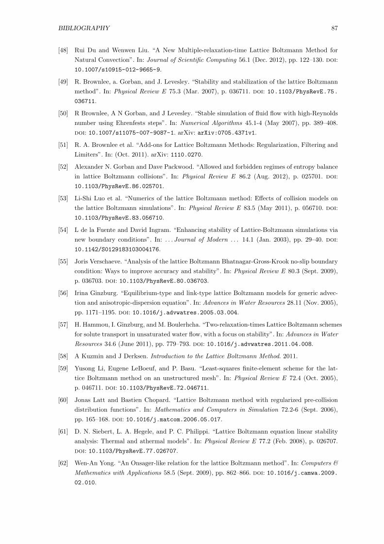
BIBLIOGRAPHY 87
[48] Rui Du and Wenwen Liu. “A New Multiple-relaxation-time Lattice Boltzmann Method for
Natural Convection”. In: Journal of Scientific Computing 56.1 (Dec. 2012), pp. 122–130. doi:
10.1007/s10915-012-9665-9.
[49] R. Brownlee, a. Gorban, and J. Levesley. “Stability and stabilization of the lattice Boltzmann
method”. In: Physical Review E 75.3 (Mar. 2007), p. 036711. doi: 10.1103/PhysRevE.75.
036711.
[50] R Brownlee, A N Gorban, and J Levesley. “Stable simulation of fluid flow with high-Reynolds
number using Ehrenfests steps”. In: Numerical Algorithms 45.1-4 (May 2007), pp. 389–408.
doi: 10.1007/s11075-007-9087-1. arXiv: arXiv:0705.4371v1.
[51] R. A. Brownlee et al. “Add-ons for Lattice Boltzmann Methods: Regularization, Filtering and
Limiters”. In: (Oct. 2011). arXiv: 1110.0270.
[52] Alexander N. Gorban and Dave Packwood. “Allowed and forbidden regimes of entropy balance
in lattice Boltzmann collisions”. In: Physical Review E 86.2 (Aug. 2012), p. 025701. doi:
10.1103/PhysRevE.86.025701.
[53] Li-Shi Luo et al. “Numerics of the lattice Boltzmann method: Effects of collision models on
the lattice Boltzmann simulations”. In: Physical Review E 83.5 (May 2011), p. 056710. doi:
10.1103/PhysRevE.83.056710.
[54] L de la Fuente and David Ingram. “Enhancing stability of Lattice-Boltzmann simulations via
new boundary conditions”. In: . . . Journal of Modern . . . 14.1 (Jan. 2003), pp. 29–40. doi:
10.1142/S0129183103004176.
[55] Joris Verschaeve. “Analysis of the lattice Boltzmann Bhatnagar-Gross-Krook no-slip boundary
condition: Ways to improve accuracy and stability”. In: Physical Review E 80.3 (Sept. 2009),
p. 036703. doi: 10.1103/PhysRevE.80.036703.
[56] Irina Ginzburg. “Equilibrium-type and link-type lattice Boltzmann models for generic advec-
tion and anisotropic-dispersion equation”. In: Advances in Water Resources 28.11 (Nov. 2005),
pp. 1171–1195. doi: 10.1016/j.advwatres.2005.03.004.
[57] H. Hammou, I. Ginzburg, and M. Boulerhcha. “Two-relaxation-times Lattice Boltzmann schemes
for solute transport in unsaturated water flow, with a focus on stability”. In: Advances in Water
Resources 34.6 (June 2011), pp. 779–793. doi: 10.1016/j.advwatres.2011.04.008.
[58] A Kuzmin and J Derksen. Introduction to the Lattice Boltzmann Method. 2011.
[59] Yusong Li, Eugene LeBoeuf, and P. Basu. “Least-squares finite-element scheme for the lat-
tice Boltzmann method on an unstructured mesh”. In: Physical Review E 72.4 (Oct. 2005),
p. 046711. doi: 10.1103/PhysRevE.72.046711.
[60] Jonas Latt and Bastien Chopard. “Lattice Boltzmann method with regularized pre-collision
distribution functions”. In: Mathematics and Computers in Simulation 72.2-6 (Sept. 2006),
pp. 165–168. doi: 10.1016/j.matcom.2006.05.017.
[61] D. N. Siebert, L. A. Hegele, and P. C. Philippi. “Lattice Boltzmann equation linear stability
analysis: Thermal and athermal models”. In: Physical Review E 77.2 (Feb. 2008), p. 026707.
doi: 10.1103/PhysRevE.77.026707.
[62] Wen-An Yong. “An Onsager-like relation for the lattice Boltzmann method”. In: Computers &
Mathematics with Applications 58.5 (Sept. 2009), pp. 862–866. doi: 10.1016/j.camwa.2009.
02.010.

BIBLIOGRAPHY 88
[63] Ahmed Mezrhab et al. “Double MRT thermal lattice Boltzmann method for simulating con-
vective flows”. In: Physics Letters A 374.34 (July 2010), pp. 3499–3507. doi: 10.1016/j.
physleta.2010.06.059.
[64] Bastien Chopard, Pascal O Luthi, and J-F Wagen. “Lattice boltzmann method for wave propa-
gation in urban microcells”. In: IEE Proceedings-Microwaves, Antennas and Propagation 144.4
(1997), pp. 251–255.
[65] R A Brownlee, Alexander N Gorban, and Jeremy Levesley. “Stabilization of the lattice Boltz-
mann method using the Ehrenfests coarse-graining idea”. In: Physical Review E 74.3 (2006),
p. 37703.
[66] Richard L Liboff. Kinetic theory: classical, quantum, and relativistic descriptions. Springer
Science & Business Media, 2003.
[67] Li-Shi Luo. “Unified Theory of Lattice Boltzmann Models for Nonideal Gases”. In: Physical
Review Letters 81.8 (Aug. 1998), pp. 1618–1621. doi: 10.1103/PhysRevLett.81.1618.
[68] P. Bhatnagar, E. Gross, and M. Krook. “A Model for Collision Processes in Gases. I. Small
Amplitude Processes in Charged and Neutral One-Component Systems”. In: Physical Review
94.3 (May 1954), pp. 511–525. doi: 10.1103/PhysRev.94.511.
[69] Irina Ginzburg, Frederik Verhaeghe, and Dominique D’Humieres. “Two-relaxation-time lattice
Boltzmann scheme: About parametrization, velocity, pressure and mixed boundary conditions”.
In: Communications in computational physics 3.2 (2008), pp. 427–478.
[70] I Ginzbourg and P M Adler. “Boundary flow condition analysis for the three-dimensional
lattice Boltzmann model”. In: Journal de Physique II 4.2 (1994), pp. 191–214.
[71] Paul Ehrenfest and Tatiana Ehrenfest. The conceptual foundations of the statistical approach
in mechanics. Courier Corporation, 1990.
[72] Shyam Chikatamarla and Iliya Karlin. “Entropy and Galilean Invariance of Lattice Boltz-
mann Theories”. In: Physical Review Letters 97.19 (Nov. 2006), p. 190601. doi: 10.1103/
PhysRevLett.97.190601.
[73] A Bardow, I V Karlin, and A A Gusev. “General characteristic-based algorithm for off-lattice
Boltzmann simulations”. In: EPL (Europhysics Letters) 75.3 (2006), p. 434.
[74] Stephen Wolfram. “Cellular automaton fluids 1: Basic theory”. In: Journal of Statistical Physics
45.3-4 (1986), pp. 471–526.
[75] Paul Lavallee, Jean Pierre Boon, and Alain Noullez. “Boundaries in lattice gas flows”. In:
Physica D: Nonlinear Phenomena 47.1 (1991), pp. 233–240.
[76] P A Skordos. “Initial and boundary conditions for the lattice Boltzmann method”. In: Physical
Review E 48.6 (1993), p. 4823.
[77] David R Noble et al. “A consistent hydrodynamic boundary condition for the lattice Boltzmann
method”. In: Physics of Fluids (1994-present) 7.1 (1995), pp. 203–209.
[78] Robert S Maier, Robert S Bernard, and Daryl W Grunau. “Boundary conditions for the lattice
Boltzmann method”. In: Physics of Fluids (1994-present) 8.7 (1996), pp. 1788–1801.
[79] Qisu Zou and Xiaoyi He. “On pressure and velocity boundary conditions for the lattice Boltz-
mann BGK model”. In: Physics of Fluids 9.6 (1997).
[80] ET Jaynes. “Information theory and statistical mechanics”. In: Physical review (1957).
[81] Claude E Shannon. “The Bell Technical Journal,”. In: A mathematical theory of communication
27.4 (1948), pp. 379–423.

BIBLIOGRAPHY 89
[82] A I Khinchin. “Mathematical Foundations of Information Theory Dover Publications Inc”. In:
New York (1957).
[83] S. Kullback and R. A. Leibler. “On Information and Sufficiency”. EN. In: The Annals of
Mathematical Statistics 22.1 (Mar. 1951), pp. 79–86.
[84] Shunsuke Ihara. Information theory for continuous systems. Vol. 2. World Scientific, 1993.
[85] I V Karlin, F Bosch, and S S Chikatamarla. “Gibbs’ principle for the lattice-kinetic theory of
fluid dynamics”. In: Physical Review E 90.3 (2014), p. 31302.
[86] Fabian Bosch, Shyam S Chikatamarla, and Ilya Karlin. “Entropic Multi-Relaxation Models for
Simulation of Fluid Turbulence”. In: arXiv preprint arXiv:1507.02509 (2015).
[87] Santosh Ansumali and Iliya V. Karlin. “Kinetic boundary conditions in the lattice Boltzmann
method”. In: Physical Review E 66.2 (Aug. 2002), p. 26311.
[88] Irina Ginzburg. “Generic boundary conditions for lattice Boltzmann models and their appli-
cation to advection and anisotropic dispersion equations”. In: Advances in Water Resources
28.11 (Nov. 2005), pp. 1196–1216. doi: 10.1016/j.advwatres.2005.03.009.
[89] Shuling Hou et al. “Simulation of Cavity Flow by the Lattice Boltzmann Method”. In: Journal
of Computational Physics 118.2 (May 1995), pp. 329–347. doi: http://dx.doi.org/10.1006/
jcph.1995.1103.


![Improving computational efficiency of lattice Boltzmann ... · 1.1 The lattice Boltzmann method The lattice Boltzmann method [7] [20] is a relative new technique to CFD. Classical](https://static.fdocuments.us/doc/165x107/5f03952b7e708231d409c3df/improving-computational-efficiency-of-lattice-boltzmann-11-the-lattice-boltzmann.jpg)


![From Lattice Boltzmann Method to Lattice Boltzmann Flux … · From Lattice Boltzmann Method to Lattice Boltzmann Flux Solver Yan Wang 1, ... flows [8,13–15], compressible flows](https://static.fdocuments.us/doc/165x107/5cadf91b88c9938f4d8c0cd6/from-lattice-boltzmann-method-to-lattice-boltzmann-flux-from-lattice-boltzmann.jpg)
