Lattice Boltzmann Methods for Fluid Structure Interaction · lattice boltzmann methods for fluid...

MONTEREY, CALIFORNIA

DISSERTATION

LATTICE BOLTZMANN METHODS FOR FLUIDSTRUCTURE INTERACTION

by

Stuart R. Blair

September 2012

Dissertation Supervisor: Young Kwon

Approved for public release; distribution is unlimited

THIS PAGE INTENTIONALLY LEFT BLANK

REPORT DOCUMENTATION PAGE Form Approved OMB No. 0704-0188

Public reporting burden for this collection of information is estimated to average 1 hour per response, including the time for reviewing instruction, searching existing data sources, gathering andmaintaining the data needed, and completing and reviewing the collection of information. Send comments regarding this burden estimate or any other aspect of this collection of information,including suggestions for reducing this burden, to Washington headquarters Services, Directorate for Information Operations and Reports, 1215 Jefferson Davis Highway, Suite 1204, Arlington,VA 22202-4302, and to the Office of Management and Budget, Paperwork Reduction Project (0704-0188) Washington DC 20503.

1. AGENCY USE ONLY (Leave blank) 2. REPORT DATESeptember 2012

3. REPORT TYPE AND DATES COVEREDDissertation

4. TITLE AND SUBTITLE: Lattice Boltzmann Methods for Fluid Struc-ture Interaction

5. FUNDING NUMBERS

6. AUTHOR(S): Stuart R. Blair

7. PERFORMING ORGANIZATION NAME(S) AND ADDRESS(ES) 8. PERFORMING ORGANIZATIONREPORT NUMBER

9.SPONSORING/MONITORING AGENCY NAME(S) AND ADDRESS(ES) 10. SPONSORING/MONITORINGAGENCY REPORT NUMBER

11. SUPPLEMENTARY NOTES: The views expressed in this thesis are those of the author and do not reflect theofficial policy or position of the Department of Defense or the U.S. Government. IRB Protocol Number: NA.

12a. DISTRIBUTION / AVAILABILITY STATEMENTApproved for public release; distribution is unlimited

12b. DISTRIBUTION CODEA

13. ABSTRACT (maximum 200 words)The use of lattice Boltzmann methods (LBM) for fluid flow and its coupling with finite element method (FEM)structural models for fluid-structure interaction (FSI) is investigated. A body of high performance LBM software thatexploits graphic processing unit (GPU) and multiprocessor programming models is developed and validated againsta set of two- and three-dimensional benchmark problems. Computational performance is shown to exceed recentlyreported results for single-workstation implementations over a range of problem sizes. A mixed-precision LBMcollision algorithm is presented that retains the accuracy of double-precision calculations with less computationalcost than a full double-precision implementation. FSI modelling methodology and example applications are presentedalong with a novel heterogeneous parallel implementation that exploits task-level parallelism and workload sharingbetween the central processing unit (CPU) and GPU that allows significant speedup over other methods. Multi-component LBM fluid models are explicated and simple immiscible multi-component fluid flows in two-dimensionsare presented. These multi-component fluid LBM models are also paired with structural dynamics solvers for two-dimensional FSI simulations. To enhance modeling capability for domains with complex surfaces, a novel couplingmethod is introduced that allows use of both classical LBM (CLBM) and a finite element LBM (FELBM) to becombined into a hybrid LBM that exploits the flexibility of FELBM while retaining the efficiency of CLBM.14. SUBJECT TERMSlattice Boltzmann method, fluid-structure interaction

15. NUMBEROF PAGES16116. PRICE CODE

17. SECURITYCLASSIFICATIONOF REPORTUnclassified

18. SECURITYCLASSIFICATIONOF THIS PAGEUnclassified

19. SECURITYCLASSIFICATIONOF ABSTRACTUnclassified

20. LIMITATION OFABSTRACTUU

NSN 7540-01-280-5500 Standard Form 298 (Rev. 2-89)Prescribed by ANSI Std. 239-18

i

Approved for public release; distribution is unlimited

LATTICE BOLTZMANN METHODS FOR FLUID STRUCTURE INTERACTION

Stuart R. BlairCommander, United States Navy

B.S., United States Naval Academy, 1994M.S., Massachusetts Institute of Technology, 2003

Nuclear Eng., Massachusetts Institute of Technology, 2003

Submitted in partial fulfillment of therequirements for the degree of

DOCTOR OF PHILOSOPHY INMECHANICAL ENGINEERING

from the

NAVAL POSTGRADUATE SCHOOLSeptember 2012

Author:Stuart R. Blair

Approved By:Young W. KwonDistinguished ProfessorDept. of Mech. & Aero. EngineeringDissertation Committee Chair

Garth V. HobsonProfessorDept. of Mech. & Aero. Engineering

Joshua H. GordisAssociate ProfessorDept. of Mech. & Aero. Engineering

Clyde L. ScandrettProfessorDept. of Applied Mathematics

Francis X. GiraldoProfessorDept. of Applied Mathematics

Approved By:Knox T. Millsaps, Professor & Chair, Dept. of Mechanical & Aerospace Engineering

Approved By:Doug Moses, Vice Provost for Academic Affairs

iii


iv

ABSTRACT

The use of lattice Boltzmann methods (LBM) for fluid flow and its coupling with finite el-

ement method (FEM) structural models for fluid-structure interaction (FSI) is investigated.

A body of high performance LBM software that exploits graphic processing unit (GPU) and

multiprocessor programming models is developed and validated against a set of two- and

three-dimensional benchmark problems. Computational performance is shown to exceed

recently reported results for single-workstation implementations over a range of problem

sizes. A mixed-precision LBM collision algorithm is presented that retains the accuracy of

double-precision calculations with less computational cost than a full double-precision im-

plementation. FSI modelling methodology and example applications are presented along

with a novel heterogeneous parallel implementation that exploits task-level parallelism and

workload sharing between the central processing unit (CPU) and GPU that allows signifi-

cant speedup over other methods. Multi-component LBM fluid models are explicated and

simple immiscible multi-component fluid flows in two-dimensions are presented. These

multi-component fluid LBM models are also paired with structural dynamics solvers for

two-dimensional FSI simulations. To enhance modeling capability for domains with com-

plex surfaces, a novel coupling method is introduced that allows use of both classical LBM

(CLBM) and a finite element LBM (FELBM) to be combined into a hybrid LBM that

exploits the flexibility of FELBM while retaining the efficiency of CLBM.

v


vi

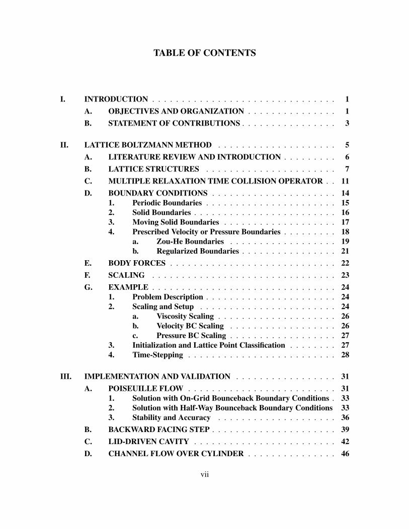
TABLE OF CONTENTS

I. INTRODUCTION . . . . . . . . . . . . . . . . . . . . . . . . . . . . . . . 1A. OBJECTIVES AND ORGANIZATION . . . . . . . . . . . . . . . 1B. STATEMENT OF CONTRIBUTIONS . . . . . . . . . . . . . . . . 3

II. LATTICE BOLTZMANN METHOD . . . . . . . . . . . . . . . . . . . . 5A. LITERATURE REVIEW AND INTRODUCTION . . . . . . . . . 6B. LATTICE STRUCTURES . . . . . . . . . . . . . . . . . . . . . . 7C. MULTIPLE RELAXATION TIME COLLISION OPERATOR . . 11D. BOUNDARY CONDITIONS . . . . . . . . . . . . . . . . . . . . . 14

1. Periodic Boundaries . . . . . . . . . . . . . . . . . . . . . . 152. Solid Boundaries . . . . . . . . . . . . . . . . . . . . . . . . 163. Moving Solid Boundaries . . . . . . . . . . . . . . . . . . . 174. Prescribed Velocity or Pressure Boundaries . . . . . . . . . 18

a. Zou-He Boundaries . . . . . . . . . . . . . . . . . . 19b. Regularized Boundaries . . . . . . . . . . . . . . . . 21

E. BODY FORCES . . . . . . . . . . . . . . . . . . . . . . . . . . . . 22F. SCALING . . . . . . . . . . . . . . . . . . . . . . . . . . . . . . . 23G. EXAMPLE . . . . . . . . . . . . . . . . . . . . . . . . . . . . . . . 24

1. Problem Description . . . . . . . . . . . . . . . . . . . . . . 242. Scaling and Setup . . . . . . . . . . . . . . . . . . . . . . . 24

a. Viscosity Scaling . . . . . . . . . . . . . . . . . . . . 26b. Velocity BC Scaling . . . . . . . . . . . . . . . . . . 26c. Pressure BC Scaling . . . . . . . . . . . . . . . . . . 27

3. Initialization and Lattice Point Classification . . . . . . . . 274. Time-Stepping . . . . . . . . . . . . . . . . . . . . . . . . . 28

III. IMPLEMENTATION AND VALIDATION . . . . . . . . . . . . . . . . . 31A. POISEUILLE FLOW . . . . . . . . . . . . . . . . . . . . . . . . . 31

1. Solution with On-Grid Bounceback Boundary Conditions . 332. Solution with Half-Way Bounceback Boundary Conditions 333. Stability and Accuracy . . . . . . . . . . . . . . . . . . . . 36

B. BACKWARD FACING STEP . . . . . . . . . . . . . . . . . . . . . 39C. LID-DRIVEN CAVITY . . . . . . . . . . . . . . . . . . . . . . . . 42D. CHANNEL FLOW OVER CYLINDER . . . . . . . . . . . . . . . 46

vii

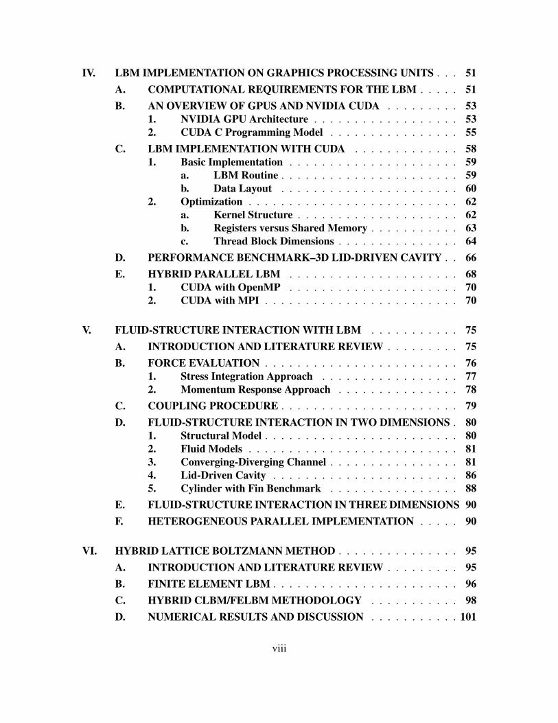
IV. LBM IMPLEMENTATION ON GRAPHICS PROCESSING UNITS . . . 51A. COMPUTATIONAL REQUIREMENTS FOR THE LBM . . . . . 51B. AN OVERVIEW OF GPUS AND NVIDIA CUDA . . . . . . . . . 53

1. NVIDIA GPU Architecture . . . . . . . . . . . . . . . . . . 532. CUDA C Programming Model . . . . . . . . . . . . . . . . 55

C. LBM IMPLEMENTATION WITH CUDA . . . . . . . . . . . . . 581. Basic Implementation . . . . . . . . . . . . . . . . . . . . . 59

a. LBM Routine . . . . . . . . . . . . . . . . . . . . . . 59b. Data Layout . . . . . . . . . . . . . . . . . . . . . . 60

2. Optimization . . . . . . . . . . . . . . . . . . . . . . . . . . 62a. Kernel Structure . . . . . . . . . . . . . . . . . . . . 62b. Registers versus Shared Memory . . . . . . . . . . . 63c. Thread Block Dimensions . . . . . . . . . . . . . . . 64

D. PERFORMANCE BENCHMARK–3D LID-DRIVEN CAVITY . . 66E. HYBRID PARALLEL LBM . . . . . . . . . . . . . . . . . . . . . 68

1. CUDA with OpenMP . . . . . . . . . . . . . . . . . . . . . 702. CUDA with MPI . . . . . . . . . . . . . . . . . . . . . . . . 70

V. FLUID-STRUCTURE INTERACTION WITH LBM . . . . . . . . . . . 75A. INTRODUCTION AND LITERATURE REVIEW . . . . . . . . . 75B. FORCE EVALUATION . . . . . . . . . . . . . . . . . . . . . . . . 76

1. Stress Integration Approach . . . . . . . . . . . . . . . . . 772. Momentum Response Approach . . . . . . . . . . . . . . . 78

C. COUPLING PROCEDURE . . . . . . . . . . . . . . . . . . . . . . 79D. FLUID-STRUCTURE INTERACTION IN TWO DIMENSIONS . 80

1. Structural Model . . . . . . . . . . . . . . . . . . . . . . . . 802. Fluid Models . . . . . . . . . . . . . . . . . . . . . . . . . . 813. Converging-Diverging Channel . . . . . . . . . . . . . . . . 814. Lid-Driven Cavity . . . . . . . . . . . . . . . . . . . . . . . 865. Cylinder with Fin Benchmark . . . . . . . . . . . . . . . . 88

E. FLUID-STRUCTURE INTERACTION IN THREE DIMENSIONS 90F. HETEROGENEOUS PARALLEL IMPLEMENTATION . . . . . 90

VI. HYBRID LATTICE BOLTZMANN METHOD . . . . . . . . . . . . . . . 95A. INTRODUCTION AND LITERATURE REVIEW . . . . . . . . . 95B. FINITE ELEMENT LBM . . . . . . . . . . . . . . . . . . . . . . . 96C. HYBRID CLBM/FELBM METHODOLOGY . . . . . . . . . . . 98D. NUMERICAL RESULTS AND DISCUSSION . . . . . . . . . . . 101

viii

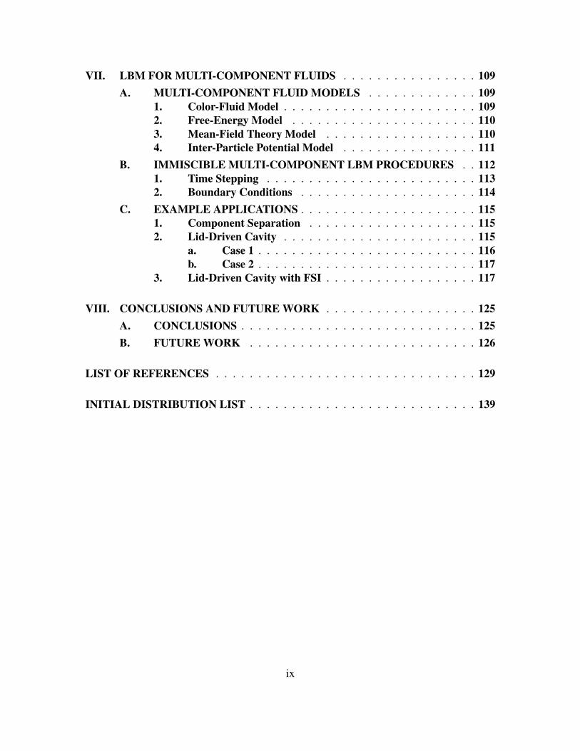
VII. LBM FOR MULTI-COMPONENT FLUIDS . . . . . . . . . . . . . . . . 109A. MULTI-COMPONENT FLUID MODELS . . . . . . . . . . . . . 109

1. Color-Fluid Model . . . . . . . . . . . . . . . . . . . . . . . 1092. Free-Energy Model . . . . . . . . . . . . . . . . . . . . . . 1103. Mean-Field Theory Model . . . . . . . . . . . . . . . . . . 1104. Inter-Particle Potential Model . . . . . . . . . . . . . . . . 111

B. IMMISCIBLE MULTI-COMPONENT LBM PROCEDURES . . 1121. Time Stepping . . . . . . . . . . . . . . . . . . . . . . . . . 1132. Boundary Conditions . . . . . . . . . . . . . . . . . . . . . 114

C. EXAMPLE APPLICATIONS . . . . . . . . . . . . . . . . . . . . . 1151. Component Separation . . . . . . . . . . . . . . . . . . . . 1152. Lid-Driven Cavity . . . . . . . . . . . . . . . . . . . . . . . 115

a. Case 1 . . . . . . . . . . . . . . . . . . . . . . . . . . 116b. Case 2 . . . . . . . . . . . . . . . . . . . . . . . . . . 117

3. Lid-Driven Cavity with FSI . . . . . . . . . . . . . . . . . . 117

VIII. CONCLUSIONS AND FUTURE WORK . . . . . . . . . . . . . . . . . . 125A. CONCLUSIONS . . . . . . . . . . . . . . . . . . . . . . . . . . . . 125B. FUTURE WORK . . . . . . . . . . . . . . . . . . . . . . . . . . . 126

LIST OF REFERENCES . . . . . . . . . . . . . . . . . . . . . . . . . . . . . . . 129

INITIAL DISTRIBUTION LIST . . . . . . . . . . . . . . . . . . . . . . . . . . . 139

ix


x

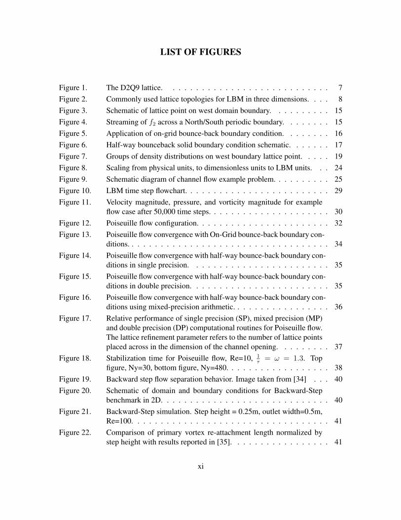
LIST OF FIGURES

Figure 1. The D2Q9 lattice. . . . . . . . . . . . . . . . . . . . . . . . . . . . 7Figure 2. Commonly used lattice topologies for LBM in three dimensions. . . . 8Figure 3. Schematic of lattice point on west domain boundary. . . . . . . . . . 15Figure 4. Streaming of f2 across a North/South periodic boundary. . . . . . . . 15Figure 5. Application of on-grid bounce-back boundary condition. . . . . . . . 16Figure 6. Half-way bounceback solid boundary condition schematic. . . . . . . 17Figure 7. Groups of density distributions on west boundary lattice point. . . . . 19Figure 8. Scaling from physical units, to dimensionless units to LBM units. . . 24Figure 9. Schematic diagram of channel flow example problem. . . . . . . . . . 25Figure 10. LBM time step flowchart. . . . . . . . . . . . . . . . . . . . . . . . . 29Figure 11. Velocity magnitude, pressure, and vorticity magnitude for example

flow case after 50,000 time steps. . . . . . . . . . . . . . . . . . . . . 30Figure 12. Poiseuille flow configuration. . . . . . . . . . . . . . . . . . . . . . . 32Figure 13. Poiseuille flow convergence with On-Grid bounce-back boundary con-

ditions. . . . . . . . . . . . . . . . . . . . . . . . . . . . . . . . . . . 34Figure 14. Poiseuille flow convergence with half-way bounce-back boundary con-

ditions in single precision. . . . . . . . . . . . . . . . . . . . . . . . 35Figure 15. Poiseuille flow convergence with half-way bounce-back boundary con-

ditions in double precision. . . . . . . . . . . . . . . . . . . . . . . . 35Figure 16. Poiseuille flow convergence with half-way bounce-back boundary con-

ditions using mixed-precision arithmetic. . . . . . . . . . . . . . . . . 36Figure 17. Relative performance of single precision (SP), mixed precision (MP)

and double precision (DP) computational routines for Poiseuille flow.The lattice refinement parameter refers to the number of lattice pointsplaced across in the dimension of the channel opening. . . . . . . . . 37

Figure 18. Stabilization time for Poiseuille flow, Re=10, 1τ

= ω = 1.3. Topfigure, Ny=30, bottom figure, Ny=480. . . . . . . . . . . . . . . . . . 38

Figure 19. Backward step flow separation behavior. Image taken from [34] . . . 40Figure 20. Schematic of domain and boundary conditions for Backward-Step

benchmark in 2D. . . . . . . . . . . . . . . . . . . . . . . . . . . . . 40Figure 21. Backward-Step simulation. Step height = 0.25m, outlet width=0.5m,

Re=100. . . . . . . . . . . . . . . . . . . . . . . . . . . . . . . . . . 41Figure 22. Comparison of primary vortex re-attachment length normalized by

step height with results reported in [35]. . . . . . . . . . . . . . . . . 41

xi

Figure 23. Schematic of the two-dimensional lid-driven cavity problem. . . . . . 42Figure 24. Lid-driven cavity in two dimensions with 1600x1600 lattice showing

from left-to-right streamlines, vorticity contours and pressure con-tours for Re=1000. Top set of figures is LBM from this work. Bottomset of figures is from [36]. . . . . . . . . . . . . . . . . . . . . . . . . 43

Figure 25. Lid-driven cavity in two dimensions with 1600x1600 lattice showingfrom left-to-right streamlines, vorticity contours and pressure con-tours for Re=5000. Top set of figures is LBM, bottom set of figuresis from [37]. . . . . . . . . . . . . . . . . . . . . . . . . . . . . . . . 43

Figure 26. Comparison of velocity, pressure and vorticity to benchmark valuesfor Re=1000. . . . . . . . . . . . . . . . . . . . . . . . . . . . . . . 45

Figure 27. Channel with cylindrical obstacle 2D problem. . . . . . . . . . . . . . 46Figure 28. Streamline visualization of trailing vortex at Re=20 (top) and Re=40

(bottom). . . . . . . . . . . . . . . . . . . . . . . . . . . . . . . . . 47Figure 29. Vorticity plot for cylinder in 2D flow at Re=100. . . . . . . . . . . . . 48Figure 30. Drag and lift coefficient for cylinder in uniform flow. Re=100. . . . . 49Figure 31. Strouhal number computed from the energy spectra of the lift coeffi-

cient at Re=100. . . . . . . . . . . . . . . . . . . . . . . . . . . . . . 49Figure 32. Historical trends for CPU and GPU memory bandwidth and compute

performance (From [52]). . . . . . . . . . . . . . . . . . . . . . . . . 52Figure 33. Memory bandwidth requirement versus desired computational through-

put for a typical LBM implementation. Modern CPU and GPU hard-ware are memory bandwidth limited for LBM. . . . . . . . . . . . . . 53

Figure 34. Simplified schematic of NVIDIA GPU. . . . . . . . . . . . . . . . . 54Figure 35. Hierarchy of threads in a CUDA program. Threads are organized into

blocks; blocks are organized into a grid (From [52]). . . . . . . . . . 55Figure 36. Schematic of data layout schemes. (a) depicts the array of structures

(AoS), (b) depicts the structure of arrays (SoA). Superscripts indicatelattice node number, subscripts indicate the lattice velocity. . . . . . . 61

Figure 37. When using SoA, load instructions executed by consecutive threadsread from consecutive locations in memory . . . . . . . . . . . . . . 61

Figure 38. Schematic of the dual lattice scheme used to support a unified timestep kernel. On even time steps, the Even Lattice is active and itcollides and streams to the Odd Lattice; vice versa for odd time steps. 63

Figure 39. LBM performance on GTX-580 for three-dimension lid-driven cavityas a function of threads per block. . . . . . . . . . . . . . . . . . . . 65

Figure 40. Performance benchmark for lattice Boltzmann method (LBM) on a3D lid-driven cavity scaled for device memory bandwidth. . . . . . . 67

xii

Figure 41. LBM on a 3D lid-driven cavity with various number of threads perblock. . . . . . . . . . . . . . . . . . . . . . . . . . . . . . . . . . . 69

Figure 42. Lid-driven cavity using a D3Q15 lattice with 5003 points using CUDAand OpenMP. . . . . . . . . . . . . . . . . . . . . . . . . . . . . . . 71

Figure 43. Schematic LBM time step for distributed computing with MPI. Scal-ability is achieved by interleaving communication with computation. . 72

Figure 44. Weak scaling using MPI for LBM simulation of three-dimensionalPoiseuille flow. . . . . . . . . . . . . . . . . . . . . . . . . . . . . . 73

Figure 45. Weak scaling using CUDA and MPI for LBM simulation of three-dimensional Poiseuille flow. . . . . . . . . . . . . . . . . . . . . . . 74

Figure 46. Euler-Bernoulli Beam. . . . . . . . . . . . . . . . . . . . . . . . . . 80Figure 47. Schematic of 2D converging and diverging duct. . . . . . . . . . . . . 82Figure 48. Converging and diverging duct displacement, velocity and accelera-

tion at beam midpoint. Re = 5, glycerin with cork beam. . . . . . . . 83Figure 49. Converging and diverging duct with combined beam response. Re=5,

glycerin with cork beam. . . . . . . . . . . . . . . . . . . . . . . . . 84Figure 50. Converging and diverging duct with varying fluid viscosity. Starting

from top left, fluid viscosity is νglycerin

4, νglycerin

2and νglycerin . . . . . . . . 85

Figure 51. Converging and diverging duct with varying beam elastic modulus.From left to right elastic modulus is Ecork

2and Ecork. . . . . . . . . . . 85

Figure 52. Schematic diagram of lid-driven cavity FSI problem geometry. . . . . 86Figure 53. Results for two-dimensional lid-driven cavity. . . . . . . . . . . . . . 87Figure 54. Final bottom displacement. . . . . . . . . . . . . . . . . . . . . . . . 88Figure 55. Cylinder with elastic fin benchmark . . . . . . . . . . . . . . . . . . 88Figure 56. Results for two-dimensional cylinder with elastic trailing fin at Re=200. 89Figure 57. Displacement, velocity and acceleration for cylinder with elastic fin.

Re=200. . . . . . . . . . . . . . . . . . . . . . . . . . . . . . . . . . 91Figure 58. Illustration of task-level decomposition in parallel implementation of

FSI problem. In the lower figure, a further level of task-level paral-lelism is exploited by overlapping the structural dynamics computa-tion on the CPU with LBM calculations on domain areas remote fromthe elastic structure on the GPU. . . . . . . . . . . . . . . . . . . . . 92

Figure 59. Decomposition of FSI problem domain for task-level heterogeneousparallelism. . . . . . . . . . . . . . . . . . . . . . . . . . . . . . . . 93

Figure 60. Schematic of Hybrid LBM time step. Methodology differs only inimplementation of the particle streaming phase. . . . . . . . . . . . . 99

xiii

Figure 61. Schematic Hybrid Lattice on regular domain. Assignment follow-ing streaming in the CLBM domain and advection in the FELBMdomain is only made to the interior of each respective sub-domain.Data drawn from the lattice points on the halo facilitates communica-tion between each sub-domain. . . . . . . . . . . . . . . . . . . . . . 99

Figure 62. Interface region for CLBM and FELBM domains on a uniform mesh.Lattice points with both the asterisk and circle belong to the interface. 100

Figure 63. Mid-channel normalized velocity profile for Poiseuille flow using CLBM,FELBM and HLBM. . . . . . . . . . . . . . . . . . . . . . . . . . . 102

Figure 64. Hybrid lattice mesh around a circular obstacle. Lattice points with as-terisk are in the CLBM sub-domain, those circled are in the FELBMsub-domain. Those with both markings are members of the interfacehalo of the two regions. . . . . . . . . . . . . . . . . . . . . . . . . . 103

Figure 65. Normalized velocity contour plot for fluid flow around circular obsta-cle at Reynolds number = 5 using CLBM . . . . . . . . . . . . . . . 104

Figure 66. Normalized velocity contour plot for fluid flow around circular obsta-cle at Reynolds number = 5 using Hybrid LBM. . . . . . . . . . . . . 105

Figure 67. Normalized velocity profile at 30 percent channel length, Reynoldsnumber = 5. . . . . . . . . . . . . . . . . . . . . . . . . . . . . . . . 106

Figure 68. Normalized velocity profile at 60 percent channel length, Reynoldsnumber = 5. . . . . . . . . . . . . . . . . . . . . . . . . . . . . . . . 107

Figure 69. Schematic Hybrid Lattice on regular domain. Assignment follow-ing streaming in the CLBM domain and advection in the FELBMdomain is only made to the interior of each respective sub-domain.Data drawn from the lattice points on the halo facilitates communica-tion between each sub-domain. . . . . . . . . . . . . . . . . . . . . . 108

Figure 70. Illustration of inter-particle forces in the nearest neighborhood of alattice point. . . . . . . . . . . . . . . . . . . . . . . . . . . . . . . . 112

Figure 71. Two immiscible components. G = -1.2 . . . . . . . . . . . . . . . . . 115Figure 72. Two immiscible components. G = -0.2. Note that the weak interaction

parameter renders the fluids miscible. . . . . . . . . . . . . . . . . . 116Figure 73. Density for Fluid 1 of a two-component immiscible fluid flow in a

lid-driven cavity. Initial configuration. . . . . . . . . . . . . . . . . . 117Figure 74. Fluid 1 results for a two-component immiscible fluid flow in a lid-

driven cavity. Sequence of images shows flow progression from topto bottom corresponding respectively to early in the simulation to itsfinal steady state. . . . . . . . . . . . . . . . . . . . . . . . . . . . . 118

xiv

Figure 75. Fluid 1 results for a two-component immiscible fluid flow in a liddriven cavity. The higher viscosity and density of fluid 2 results in itsconfinement in the bottom-half of the cavity domain. . . . . . . . . . 119

Figure 76. Fluid 1 results for a two-component immiscible fluid flow in a liddriven cavity. The higher viscosity and density of fluid 2 results in itsconfinement in the bottom-half of the cavity domain. . . . . . . . . . 119

Figure 77. Schematic representation of a lid-driven cavity with an elastic beamattached to the lower surface. . . . . . . . . . . . . . . . . . . . . . . 120

Figure 78. Single-component fluid flow in cavity with beam. Streamlines showdevelopment of three distinct vortex regions. . . . . . . . . . . . . . . 121

Figure 79. Momentum and density fields for fluid 1 at steady-state; Re=1000. . . 122Figure 80. Plot of displacement, velocity and acceleration at the tip of the elastic

beam. . . . . . . . . . . . . . . . . . . . . . . . . . . . . . . . . . . 122Figure 81. Final beam displacement for multi-component FSI. Beam displace-

ment is magnified 10 times for clarity. . . . . . . . . . . . . . . . . . 123

xv


xvi

LIST OF TABLES

Table 1. Geometry and fluid parameters for Poiseuille flow test case. . . . . . 32Table 2. Comparison of trailing vortex length to benchmark values. . . . . . . 46Table 3. Comparison of Strouhal number to benchmark values. . . . . . . . . 48Table 4. Memory bandwidth of various CUDA memory spaces on an NVIDIA

GTX-580 GPU . . . . . . . . . . . . . . . . . . . . . . . . . . . . . 64Table 5. Properties of GPU devices used in benchmark computations in Figure

40 . . . . . . . . . . . . . . . . . . . . . . . . . . . . . . . . . . . . 67Table 6. Selected structural material properties used for fluid-structure interaction

(FSI) simulations. . . . . . . . . . . . . . . . . . . . . . . . . . . . . 81Table 7. Selected fluid properties for FSI simulations. . . . . . . . . . . . . . . 81Table 8. Performance improvement from using overlapped execution depicted

in lower half of Figure 58 versus the non-overlapped scheme in thetop half of Figure 58. The lattice was 22 x 337 x 526 D3Q19 usingMRT collision operator. The structural model was a sheer-deformableplate with 2883 degrees of freedom. . . . . . . . . . . . . . . . . . . 94

Table 9. Performance comparison of CLBM and FELBM. . . . . . . . . . . . 106

xvii


xviii

LIST OF ACRONYMS AND NOMENCLATURE

API application programming interface

AoS array of structures

BGK Bhatnagar-Gross-Krook

CLBM classical lattice Boltzmann method

CUDA Compute Unified Device Architecture

DEM discrete element method

LBM lattice Boltzmann method

FELBM finite element lattice Boltzmann method

FEM finite element method

FSI fluid-structure interaction

FVM finite volume method

GB gigabytes

GFLOPS billion floating point operations per second

GPU graphical processing unit

HLBM hybrid lattice Boltzmann method

IB immersed boundary

LBGK lattice Bhatnagar-Gross-Krook

MPI message passing interface

MRT multiple relaxation time

SM Streaming Multiprocessor

SP Scalar Processors

SoA structure of arrays

VTK Visualization Toolkit

xix

cs lattice Boltzmann method lattice sound speed

eα lattice velocity

fα particle density distribution function

f eqα equilibrium density distribution function

M particle moment transformation operator

ν kinematic viscosity

Ωα collision operator

p macroscopic pressure

ρ macroscopic density

R particle moment space

S multiple relaxation time relaxation matrix

τ relaxation time

u macroscopic velocity

ω single relaxation-time relaxation operator

wα lattice weight

xx

I. INTRODUCTION

The present thesis investigates the use of the lattice Boltzmann method (LBM) to

solve for the flow of viscous, incompressible fluids while accounting for the effect these

fluid flows have on surrounding elastic structures. From waves slapping against ship struc-

tural members, cooling water passing over heat-exchanger tubes to blood flowing within

veins and arteries among many others, FSI has applications that span the engineering and

life sciences. Towards the goal of simulating such physical behavior, several intermediate

steps were required. These intermediate steps start with the development of a robust and

highly capable software tool for simulating and analyzing flow of incompressible viscous

fluids and continue through to integration of these tools with structural dynamics solvers.

A. OBJECTIVES AND ORGANIZATION

The first objective is to develop software tools required for a LBM flow solver

that can reliably and accurately simulate fluid flow problems of interest. The theory and

formulation of the LBM, including detailed considerations of stability, accuracy and proper

scaling of simulation variables to allow modeling of specific fluid systems is provided in

Chapter II.

With a detailed understanding of the theory, software tools can be developed to

simulate fluid flows of interest. Such software is developed and subjected to a collection

of validation benchmarks in Chapter III. The second-order convergence of the LBM along

with select boundary conditions is demonstrated along with a demonstration of the potential

impacts of the wide use of single-precision arithmetic on this convergence rate. A mixed-

precision LBM implementation is introduced that provides for second-order convergence

for select boundary conditions while retaining some of the performance benefits of using

single precision number representation and arithmetic.

1

In order to increase the accuracy of a LBM simulation, the spatial and temporal dis-

cretization is refined. Smaller time steps and a more refined lattice both lead to increased

computational demand. In order to execute LBM simulations in a reasonable amount of

time, the programs are written to be executed in parallel. In Chapter IV the Compute Uni-

fied Device Architecture (CUDA) programming model is introduced and the implementa-

tion of the LBM programs for parallel execution on a graphical processing unit (GPU) is

described. The achieved performance is compared with recently published benchmarks.

Two hybrid programming models are also demonstrated that use a combination of CUDA

and OpenMP in one case and CUDA and message passing interface (MPI) in another.

Collectively, Chapter IV describes the development of a scalable high-performance LBM

solver.

Once reliable fluid simulation tools are in place, the second objective is to couple

this fluid solver with an appropriate structural dynamics model. These software compo-

nents are then used as coupled FSI simulation tools. The key ingredients of computing

forces and moments along the fluid-structure interface and accounting for their exchange

and integrating with a structural dynamics solver for a coordinated FSI simulation are dis-

cussed. The specific methods and algorithms for doing this along with example applications

in both two and three dimensions are presented in Chapter V.

The aforementioned software tools were all developed based on the classical LBM

theory. A recently developed modification, termed the finite element lattice Boltzmann

method (FELBM), allows use of unstructured non-uniform finite element grids in lieu of

the regular structured grid from classical lattice Boltzmann method (CLBM). The FELBM

gains this flexibility at the expense of some computational efficiency on a per-lattice-point

basis. An algorithm and associated software tool has been developed resulting in a hybrid

lattice Boltzmann method (HLBM) whereby both CLBM and FELBM are used on disjoint

sub-domains of an overall simulation. This hybrid tool leverages the simplicity and effi-

ciency of the CLBM while also benefiting from the geometric flexibility of the FELBM.

The overall system is able to simulate fluid flow over the combined domain with less com-

2

putational effort than the FELBM while reducing the memory requirements of an equiv-

alent simulation using only CLBM. The theory and algorithms for accomplishing this is

provided in Chapter VI.

The last objective of this model is to take advantage of the flexible and physically

intuitive methods for modeling multi-component fluid systems using LBM. A discussion

of the standard LBM theory for multi-component fluids as well as example problems in

fluid flow and FSI are demonstrated in Chapter VII.

In Chapter VIII, conclusions and prospects for future research are discussed.

B. STATEMENT OF CONTRIBUTIONS

The principal contributions of this thesis are:

• A body of software tools that provide LBM modeling capability for single-

component incompressible viscous flows in two and three dimensions.

• A new mixed-precision LBM implementation that retains most of the ac-

curacy of double precision while requiring only the memory of single pre-

cision.

• A GPU-accelerated implementation of LBM with highly competitive per-

formance against recently published benchmarks.

• A new method to simulate two-way FSI that exploits task-level concur-

rency for a heterogeneous-parallel algorithm using both GPU for the fluid

domain and central processing units for the solid domain.

• A novel method for combining CLBM and FELBM into a HLBM.

• LBM flow and FSI modeling capability for multi-component flows in two

dimensions.

3


4

II. LATTICE BOLTZMANN METHOD

The LBM is an increasingly popular way to simulate fluid flow. In contrast to

more conventional methods such as finite difference methods (FDM) control volume meth-

ods (CVM) and finite element methods (FEM), the LBM begins not with the picture of

the fluid as a continuous medium, but instead as a collection of particles. These parti-

cles move and undergo local interactions with other particles in accordance with simple

rules. Macroscopic physical phenomena such as those conservation laws described by the

Navier-Stokes equations emerge from the large number of these local interactions. The

microscopic level of description provides an intuitive basis for generalization to complex

systems such as porous media ([1]-[3]), two-phase flow ([4]-[6]) and magnetohydrodynam-

ics ([7]-[9]) among others. By judiciously altering the formulation, other partial differen-

tial equations of interest have been modeled by a similar procedure including the Burgers

Equation [10], the Korteweg-de Vries equation [11], the Brinkman equation [12] and the

Schrodinger equation [13]. For a concise review of the current state of the art in LBM, an

excellent survey can be found in [14] with a recent update in [15]. A recently published

analysis of LBM theory, which includes a thorough critique and comparison with tradi-

tional computational fluid dynamics techniques, can be found at [16]. In this work, the

LBM will be used for the solution of the Navier-Stokes equations for single-component

fluid flows as well as a limited number of multi-component fluid flows.

This chapter will start with a brief overview of the historical development of the

LBM. This will be followed by a description of each element of a LBM simulation in-

cluding typical lattice structures with lattice velocities and associated weights, collision

operators, boundary conditions, body forces and scaling requirements. The chapter will

be concluded with a detailed example application of the LBM to two-dimensional channel

flow over a cylindrical obstacle.

5

A. LITERATURE REVIEW AND INTRODUCTION

Historically, the LBM is derived from the concepts of the cellular automaton [17],

[18]. Space is described by a regular array of interconnecting lattice sites and time is di-

vided into equally spaced time-steps. The cellular automata model is specified by stating

the rules by which each lattice site shall be updated for the next time step. Depending on

these rules, complex physical phenomena emerge [19]. A classical example of complex be-

havior emerging from simple rules is Conway’s Game of Life. In some cases, the CA with

associated sets of update rules have become useful as a model for real physical behavior

and have become a means to gaining more fundamental understanding. Examples include

traffic flow [20], population dynamics [21], and earthquake prediction [22] to name but a

few.

The CA model underlying a fluid dynamics model incorporates movement of par-

ticles from one lattice site to another along discrete lattice directions. The rule for lattice

site update is applied to all particles arriving at a given lattice site in a given time step and

is represented formally in Equation 1,

Nα (x + δxeα, t+ δt) = Nα (x, t) + Ωα(N) (1)

where Nα is a Boolean variable indicating the presence or absence of a fluid particle trav-

eling along lattice direction eα at position x. The rules for update—referred to as the

Collision Operator—are formally denoted by Ωα(N). One advantage of this formulation

using Boolean variables is the absence of round-off errors; all arithmetic is exact. Unfor-

tunately, though the mathematical operations are simple and exact, it has been found that

they are required in enormous numbers to overcome statistical noise in the results. Ad-

ditionally, it has been found that further lattice symmetry requirements need to be met in

order to provide Galilean invariance.

The LBM emerged from the solutions presented to these difficulties [18], [23]. The

LBM seeks to solve the discrete Boltzmann equation which, in the absence of external

6

forces is:∂fα∂t

+ eα · ∇fα = Ωα , α ∈ [0, . . . , q] , eα ∈ Rd (2)

where fα is the particle velocity distribution function for lattice direction α; eα is the set of

lattice velocities; and Ωα is the collision operator. Additionally, initial values for all fα must

be supplied on the problem domain and boundary conditions must be applied appropriately.

In the following sections, each of these issues will be addressed in turn so that a simulation

of fluid flow may be undertaken using the LBM.

B. LATTICE STRUCTURES

In the LBM, this solution is sought on a regular lattice. A lattice is defined by a

sound speed cs, a set of d-dimensional lattice velocities eα where α ∈ [0, . . . , q] and a set

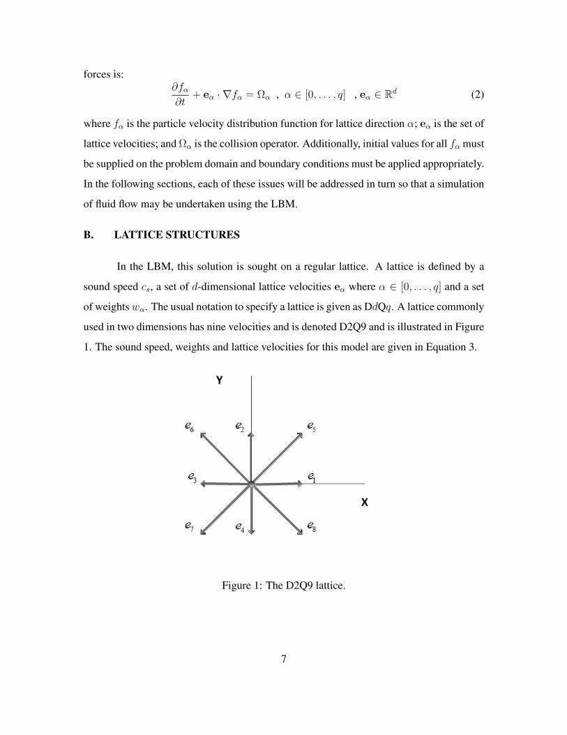
of weightswα. The usual notation to specify a lattice is given as DdQq. A lattice commonly

used in two dimensions has nine velocities and is denoted D2Q9 and is illustrated in Figure

1. The sound speed, weights and lattice velocities for this model are given in Equation 3.

Figure 1: The D2Q9 lattice.

7

c2s = 1

3

w0 = 29

w1−4 = 19

w5−8 = 136

e0 = (0, 0)

e1 = (1, 0) e2 = (0, 1) e3 = (−1, 0) e4 = (0,−1)

e5 = (1, 1) e6 = (−1, 1) e7 = (−1,−1) e8 = (1,−1)

(3)

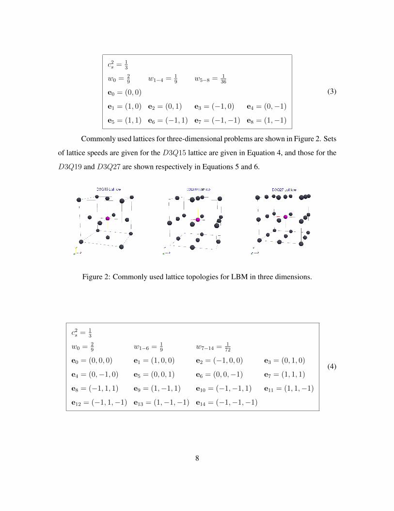
Commonly used lattices for three-dimensional problems are shown in Figure 2. Sets

of lattice speeds are given for the D3Q15 lattice are given in Equation 4, and those for the

D3Q19 and D3Q27 are shown respectively in Equations 5 and 6.

Figure 2: Commonly used lattice topologies for LBM in three dimensions.

c2s = 1

3

w0 = 29

w1−6 = 19

w7−14 = 172

e0 = (0, 0, 0) e1 = (1, 0, 0) e2 = (−1, 0, 0) e3 = (0, 1, 0)

e4 = (0,−1, 0) e5 = (0, 0, 1) e6 = (0, 0,−1) e7 = (1, 1, 1)

e8 = (−1, 1, 1) e9 = (1,−1, 1) e10 = (−1,−1, 1) e11 = (1, 1,−1)

e12 = (−1, 1,−1) e13 = (1,−1,−1) e14 = (−1,−1,−1)

(4)

8

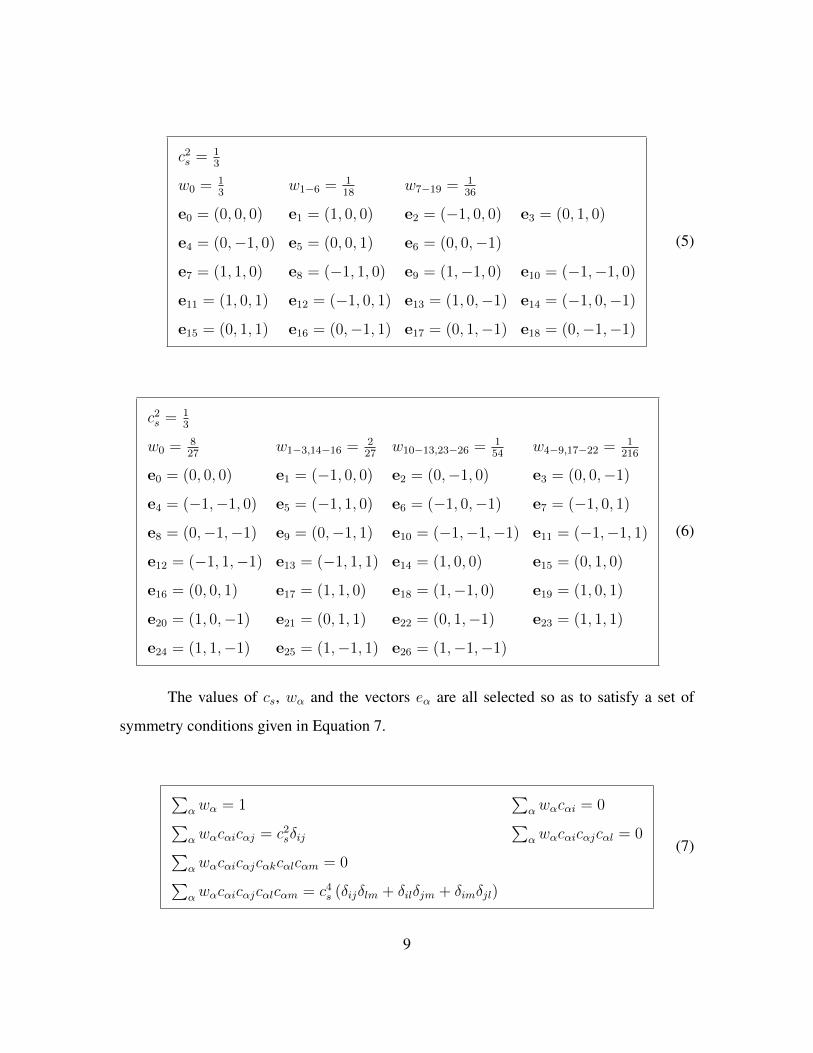
c2s = 1

3

w0 = 13

w1−6 = 118

w7−19 = 136

e0 = (0, 0, 0) e1 = (1, 0, 0) e2 = (−1, 0, 0) e3 = (0, 1, 0)

e4 = (0,−1, 0) e5 = (0, 0, 1) e6 = (0, 0,−1)

e7 = (1, 1, 0) e8 = (−1, 1, 0) e9 = (1,−1, 0) e10 = (−1,−1, 0)

e11 = (1, 0, 1) e12 = (−1, 0, 1) e13 = (1, 0,−1) e14 = (−1, 0,−1)

e15 = (0, 1, 1) e16 = (0,−1, 1) e17 = (0, 1,−1) e18 = (0,−1,−1)

(5)

c2s = 1

3

w0 = 827

w1−3,14−16 = 227

w10−13,23−26 = 154

w4−9,17−22 = 1216

e0 = (0, 0, 0) e1 = (−1, 0, 0) e2 = (0,−1, 0) e3 = (0, 0,−1)

e4 = (−1,−1, 0) e5 = (−1, 1, 0) e6 = (−1, 0,−1) e7 = (−1, 0, 1)

e8 = (0,−1,−1) e9 = (0,−1, 1) e10 = (−1,−1,−1) e11 = (−1,−1, 1)

e12 = (−1, 1,−1) e13 = (−1, 1, 1) e14 = (1, 0, 0) e15 = (0, 1, 0)

e16 = (0, 0, 1) e17 = (1, 1, 0) e18 = (1,−1, 0) e19 = (1, 0, 1)

e20 = (1, 0,−1) e21 = (0, 1, 1) e22 = (0, 1,−1) e23 = (1, 1, 1)

e24 = (1, 1,−1) e25 = (1,−1, 1) e26 = (1,−1,−1)

(6)

The values of cs, wα and the vectors eα are all selected so as to satisfy a set of

symmetry conditions given in Equation 7.

∑αwα = 1

∑αwαcαi = 0∑

αwαcαicαj = c2sδij

∑αwαcαicαjcαl = 0∑

αwαcαicαjcαkcαlcαm = 0∑αwαcαicαjcαlcαm = c4

s (δijδlm + δilδjm + δimδjl)

(7)

9

These symmetry conditions play an important roll in the theory of LBM. In particular, they

are needed to show the correspondence between the LBM and the incompressible Navier-

Stokes equation. It can be shown that all of the lattices introduced satisfy these conditions.

The discrete Boltzmann Equation shown in Equation 2 is in the general form of an

advection equation. The momentum space is discretized along the q lattice speeds which,

with the advection equation analogy, are the characteristic speeds. The right hand side of

Equation 2 is the collision operator Ωα which determines what happens to the particle pop-

ulations fα as they traverse the lattice in their respective characteristic directions. Instead

of numerically integrating the temporal and spatial derivative operators, the LBM handles

them discretely in time and space by “streaming” particle distributions from a source lattice

site to neighboring lattice site in each direction. This process is illustrated schematically

with the arrows in in Figure 1 and is formally expressed in Equation 8 where r is the posi-

tion vector for a given lattice point and t is the current time in lattice units.

fα (r + eα, t+ 1)− fα (r, t) = Ωα. (8)

The simplest and most popular form for the collision operator is the Bhatnagar-

Gross-Krook (BGK), shown in Equation 9, which gives a single-parameter relaxation to

equilibrium:

ΩBGKα = −1

τ(fα − f eqα ) (9)

where τ is a relaxation parameter, f eqα is a function of the macroscopic parameters of the

fluid represented by fα given by Equation 10.

f eqα = ρwα

[1 +

(eα · u)

c2s

+(eα · u)2

c4s

− 1

2

(u · u)

c2s

](10)

The macroscopic variables of fluid density and velocity, given by ρ and u, respectively, are

10

computed as moments of the particle distribution function fα as shown in Equations 11 and

12. When required for physical modeling, the fluid pressure p can also be obtained from

Equation 13.

ρ =

q−1∑α=0

fα (11)

u =1

ρ

q−1∑α=0

fαeα (12)

p = ρc2s (13)

The relaxation parameter τ can be related to the fluid kinematic viscosity ν. This relation-

ship is given in Equation 14 with all units expressed in lattice units.

τ =ν

c2s

+1

2(14)

Frequently in the literature, and periodically in this thesis, the inverse of τ is used

as the relaxation parameter and is conventionally named ω. Since for real fluids, ν must

be non-negative, τ is constrained to be greater than or equal to 12. In notation employing

ω, this implies 0 ≤ ω ≤ 2. In a later section of this thesis where dimensional scaling

and stability are discussed, it will be demonstrated that the numerical stability of any given

LBM simulation can be characterized by the value of τ or ω. Systems where the combined

fluid properties, boundary conditions and LBM spatial and temporal discretizations result in

the value of ω to be close to 2, or conversely τ approaching 12, tend to become numerically

unstable.

C. MULTIPLE RELAXATION TIME COLLISION OPERATOR

While the single relaxation time lattice Bhatnagar-Gross-Krook (LBGK) operator

is easy to implement and computationally efficient within the context of a single LBM time

11

step, it is known to suffer from severe stability problems. When these stability problems

can be overcome while still using LBGK, it is often only obtained at the expense of an

increase in lattice density and hence, increase in computational effort. The LBGK has other

deficiencies including an implied fixed Prandtl number of one and a fixed ratio between

kinematic and bulk viscosity. In order to provide a means for tuning the stability properties

of a given simulation while also a mechanism for altering more specific fluid properties,

alternative collision operators have been developed.

The multiple relaxation time (MRT) collision operator, also referred to as the gener-

alized lattice Boltzmann equation, was first presented in [24]. Its objectives were to resolve

the fixed Prandtl number defect of LBGK, and allow for varying kinematic and bulk vis-

cosities as well as introduce a mechanism for increasing simulation stability. The MRT

projects the density distribution functions fα onto an orthogonal vector space of momenta

of the vector space using the operator M. The particular momenta depend on the lattice

structure chosen but all include a combination of the mass density, kinetic energy, mo-

mentum flux, energy flux and viscous stress tensor. They are expressed in the vector R.

Relaxation occurs over the momentum space using the relaxation times given in S and the

result is transformed back to the density space fα using the inverse of M.

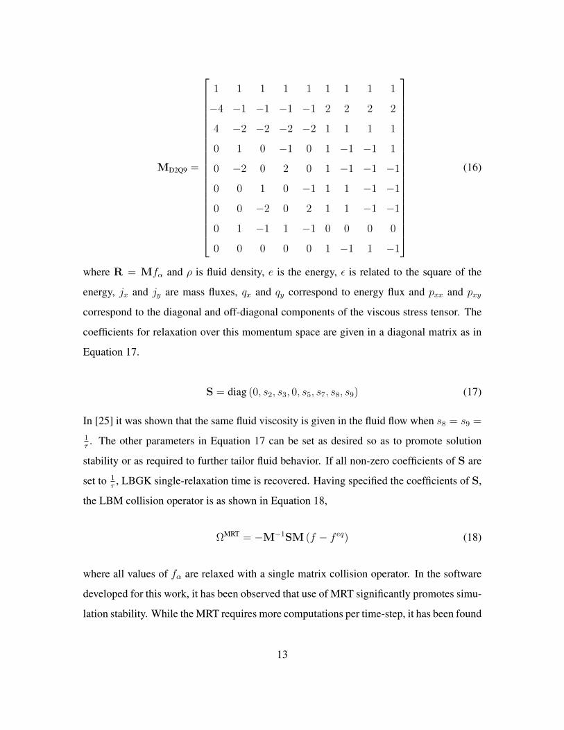
For the D2Q9 lattice, the momentum space and transformation matrix are given in

Equations 15 and Equation 16, respectively.

RD2Q9 =[ρ e ε jx qx jy qy pxx qxy

]T(15)

12

MD2Q9 =

1 1 1 1 1 1 1 1 1

−4 −1 −1 −1 −1 2 2 2 2

4 −2 −2 −2 −2 1 1 1 1

0 1 0 −1 0 1 −1 −1 1

0 −2 0 2 0 1 −1 −1 −1

0 0 1 0 −1 1 1 −1 −1

0 0 −2 0 2 1 1 −1 −1

0 1 −1 1 −1 0 0 0 0

0 0 0 0 0 1 −1 1 −1

(16)

where R = Mfα and ρ is fluid density, e is the energy, ε is related to the square of the

energy, jx and jy are mass fluxes, qx and qy correspond to energy flux and pxx and pxy

correspond to the diagonal and off-diagonal components of the viscous stress tensor. The

coefficients for relaxation over this momentum space are given in a diagonal matrix as in

Equation 17.

S = diag (0, s2, s3, 0, s5, s7, s8, s9) (17)

In [25] it was shown that the same fluid viscosity is given in the fluid flow when s8 = s9 =

1τ. The other parameters in Equation 17 can be set as desired so as to promote solution

stability or as required to further tailor fluid behavior. If all non-zero coefficients of S are

set to 1τ, LBGK single-relaxation time is recovered. Having specified the coefficients of S,

the LBM collision operator is as shown in Equation 18,

ΩMRT = −M−1SM (f − f eq) (18)

where all values of fα are relaxed with a single matrix collision operator. In the software

developed for this work, it has been observed that use of MRT significantly promotes simu-

lation stability. While the MRT requires more computations per time-step, it has been found

13

that simulations are able to be conducted with much lower lattice density. Furthermore,

fewer time steps are typically required for flows to overcome the noise of nonequilibrium

initial conditions and reach accurate flow configurations.

D. BOUNDARY CONDITIONS

The fluid flow problems which we hope to solve using LBM are initial boundary

value problems. As such, the handling of initial and boundary conditions should be central

to any discourse on numerical solution methods.

One problem with LBM is that the physically relevant and observable macroscopic

flow features such as velocity and pressure are not the dependent variables in the governing

equation; rather they are functions of the dependent variables. While it is possible to find a

reasonable set of fα corresponding to a particular pressure and velocity there is in general

no unique way to do this.

Despite this difficulty, researchers have formulated numerous schemes that try to

view the boundary lattice points in a manner consistent with every other lattice point with

the exception that, for certain lattice directions there is no updated data streamed in from

the previous time step. This condition is illustrated schematically in Figure 3.

The boundary condition schemes described in this section represent answers to the

dual questions:

1. What value should be given for each fα for which there is not a corre-

sponding neighbor?

2. How can this be done so as the desired macroscopic boundary condition

will be enforced?

The boundary conditions discussed in this section answer these questions. The dis-

cussion will not survey all available methods, but only those implemented for this research.

Each method will be examined on the basis of stability and implementation effectiveness.

14

Figure 3: Schematic of lattice point on west domain boundary.

1. Periodic Boundaries

Periodic boundary conditions are a common and easy to implement boundary con-

dition with LBM. For nodes along a periodic boundary, the node along the corresponding

periodic boundary is assigned as the nearest neighbor for streaming purposes. The density

distribution for that direction is replaced accordingly as is shown in Figure 4.

Figure 4: Streaming of f2 across a North/South periodic boundary.

15

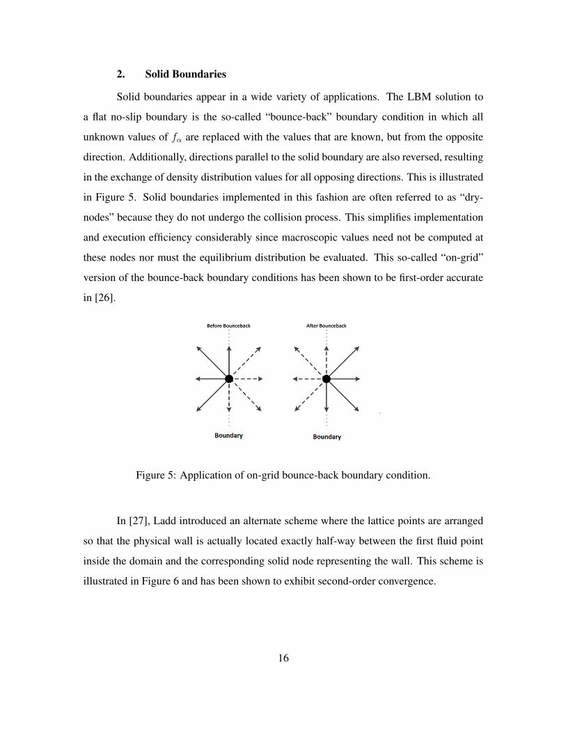
2. Solid Boundaries

Solid boundaries appear in a wide variety of applications. The LBM solution to

a flat no-slip boundary is the so-called “bounce-back” boundary condition in which all

unknown values of fα are replaced with the values that are known, but from the opposite

direction. Additionally, directions parallel to the solid boundary are also reversed, resulting

in the exchange of density distribution values for all opposing directions. This is illustrated

in Figure 5. Solid boundaries implemented in this fashion are often referred to as “dry-

nodes” because they do not undergo the collision process. This simplifies implementation

and execution efficiency considerably since macroscopic values need not be computed at

these nodes nor must the equilibrium distribution be evaluated. This so-called “on-grid”

version of the bounce-back boundary conditions has been shown to be first-order accurate

in [26].

Figure 5: Application of on-grid bounce-back boundary condition.

In [27], Ladd introduced an alternate scheme where the lattice points are arranged

so that the physical wall is actually located exactly half-way between the first fluid point

inside the domain and the corresponding solid node representing the wall. This scheme is

illustrated in Figure 6 and has been shown to exhibit second-order convergence.

16

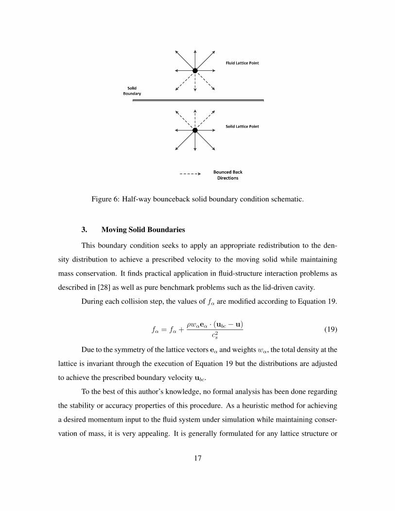
Figure 6: Half-way bounceback solid boundary condition schematic.

3. Moving Solid Boundaries

This boundary condition seeks to apply an appropriate redistribution to the den-

sity distribution to achieve a prescribed velocity to the moving solid while maintaining

mass conservation. It finds practical application in fluid-structure interaction problems as

described in [28] as well as pure benchmark problems such as the lid-driven cavity.

During each collision step, the values of fα are modified according to Equation 19.

fα = fα +ρwαeα · (ubc − u)

c2s

(19)

Due to the symmetry of the lattice vectors eα and weightswα, the total density at the

lattice is invariant through the execution of Equation 19 but the distributions are adjusted

to achieve the prescribed boundary velocity ubc.

To the best of this author’s knowledge, no formal analysis has been done regarding

the stability or accuracy properties of this procedure. As a heuristic method for achieving

a desired momentum input to the fluid system under simulation while maintaining conser-

vation of mass, it is very appealing. It is generally formulated for any lattice structure or

17

location within the domain and in fluid simulations where it has been used for this work, it

has shown excellent stability properties. As for accuracy, it was used in the lid-driven cav-

ity benchmark discussed in Chapter III where it is shown to allow for excellent agreement

with both experimental and computational data reported in the literature.

4. Prescribed Velocity or Pressure Boundaries

Prescribed velocity and pressure boundary conditions constitute an indispensable

tool for fluid modeling problems. As with other boundary condition schemes, the methods

to be described in this section all seek to assign suitable values to fα for lattice points

along a boundary so that the desired macroscopic conditions are realized. An excellent

review paper can be found at [29] that formally analyzes several methods. Details included

in this section are drawn largely from this reference. A common theme among boundary

conditions of this type is that specification of either density—which in the LBM framework

is equivalent to pressure by using Equation 13—or velocity, the other macroscopic variable

can be determined based solely on the known values of fα.

Referring to Figure 7, the contributors to the macroscopic density at a lattice point

can be grouped into three categories: those stationary or parallel to the boundary ρ0 - f0, f2,

and f4 in this case; those known density distributions pointed into the boundary ρ+ - f3,f6,

and f7; and those pointed out from the boundary ρ− - f1,f5 and f8. Every straight boundary

will have this grouping. Comparing this with Equation 11, it can be seen that Equation 20 is

an identity. Additionally, considering the lattice velocities it is easy to demonstrate that the

velocity component perpendicular to the straight boundary can be expressed as in Equation

21.

ρ = ρ− + ρ0 + ρ+ (20)

ρu⊥ = ρ+ − ρ− (21)

Given Equations 20 and 21, given either the value for the velocity component into the

domain, u⊥ or ρ, it is always possible to determine the other using only the density distri-

bution components that are known after streaming - ρ0 and ρ+. These relations are given in

18

Figure 7: Groups of density distributions on west boundary lattice point.

Equations 22 and 23.

ρ =1

1 + u⊥(2ρ+ + ρ0) (22)

u⊥ = −1 +(2ρ+ + ρ0)

ρ(23)

Once the value for ρ and u are known on the boundary, this information can be used to

judiciously assign values either to the unknown density distributions as in the Zou-He type

boundary conditions [30] or, in the case of the regularized boundary conditions introduced

in [31], to all distributions.

a. Zou-He Boundaries

The Zou-He scheme for prescribed pressure or velocity seek to find suitable

values only for the unknown density distributions at the boundary lattice point. For this ex-

ample, the case of a prescribed-velocity boundary condition on the West domain boundary

as depicted in Figure 7 will be used.

19

For the condition depicted, when accounting for the prescribed velocity on

the boundary, there remain four unknowns: ρ, f1, f5 and f8. Balanced against these four

unknowns is the known relation for density given in Equation 11, and two equations for

momentum given by Equation 12. In order to provide closure, a fourth relationship is nec-

essary. The Zou-He boundary conditions develop this relationship by assuming “bounce-

back” of the non-equilibrium part of the density distribution directed perpendicular to the

boundary. In this case, this gives us Equation 24.

f1 − f neq1 = f3 − f neq

3 (24)

Applying Equation 10 along with the known ρ and u and appropriate lattice vectors e1 and

e3 and weights w1, w3, the above relation simplifies to Equation 25

f1 = f3 +2

3ρux (25)

In two dimensions, this provides closure and values of the remaining unknown density

distribution functions can be determined. For this example, the expressions are given as

Equation 26 and Equation 27.

f5 = f7 +1

2(f4 − f2) +

1

2ρuy +

1

6ρux (26)

f8 = f6 −1

2(f4 − f2)− 1

2ρuy +

1

6ρux (27)

For prescribed pressure, the procedure is the same, except that given ρ, we solve for u⊥ -

in this case ux.

For three dimensions, there are still more unknowns; using the D3Q15 lat-

tice and applying a boundary condition to the west domain boundary, In addition to one of

ρ or u⊥, there are five density distributions that are unknown: f1,f7,f9,f11 and f13. In the

case of the D3Q27 lattice, there are nine unknown density distribution functions.

20

The idea demonstrated in [32] is to apply the non-equilibrium bounce-back

as used in Equation 24 to all unknown density distribution values relative to the known

density distribution in the opposite direction. If we adopt the convention that for a given

density distribution fk, fk connotes the density distribution traveling in the opposite direc-

tion, and fk is an unknown density distribution, this is shown in Equation 28 for the D3Q15

lattice.

fk = fk +(f eqk − f

eq

k

), k ∈ 1, 7, 9, 11, 13 (28)

In order to correct for momenta in the plane of the boundary—for this example, in the y and

z directions—an adjustment is applied to the density distributions that are not perpendicular

to the boundary, which is shown in Equation 29 for the D3Q15 lattice.

fk = fk +1

4[eky (f3 − f4) + ekz (f5 − f6)] , k ∈ 7, 9, 11, 13 (29)

Putting this all together, we arrive at Equations 30 and 31.

f1 = f2 +2

3ρinux (30)

fk = fk +1

12ρinux −

1

4[eky (f3 − f4) + ekz (f5 − f6)] , k ∈ 7, 9, 11, 13 (31)

For other lattice types and other boundaries, the same general prescription is followed.

b. Regularized Boundaries

For regularized boundary conditions, introduced in [31] and discussed in

more detail in [29], all particle distribution functions on boundary lattice points are replaced

based on values of ρ, u or Π(1) that are either specified by the boundary condition or

computed based on known particle distribution values.

21

In the same fashion as with the Zou-He boundary condition, given either

ρ or u⊥, the other macroscopic variable can be determined based on the known values

of fα. Once this is complete, f eqα is computed using Equation 10. Values for the unknown

density distribution function—fk—are initially estimated based on bounce-back of the non-

equilibrium parts as in Equation 28. Since we cannot know the non-equilibrium portion of

fk, we simply assign it to have the same non-equilibrium component as fk as shown in

Equation 32.

fk = f eqk + fk − feq

k(32)

The tensor Π is the second-order moment of the particle density populations and can be

expressed as in Equation 33.

Π =

q−1∑α=0

eαeαfα (33)

Equation 34 is used to reconstruct hydrodynamically consistent values for all fα on the

boundary lattice point,

fα = f eqα +wα2c4s

Qα : Π (34)

where Qα = eαeα − c2sI, I being the identity matrix. This method for boundary condition

application is appealing for its generality. The superior stability properties of this method

is discussed at length in [29] and [31].

E. BODY FORCES

Many physical simulations require the application of a body force. Some simple

examples would be a simulation that includes gravity; a simulation with an imposed dif-

ferential pressure, where the pressure is included as a body force on the fluid particles; or

a multi-component model where the interaction between particles of different species are

22

modeled by nearest-neighbor force inputs. The most common way to incorporate these

forces is via an adjustment to the equilibrium velocity as given in Equation 35,

ueq = u + ∆u (35)

where ∆u is given by Equation 36.

∆u =τF

ρ(36)

Equation 36 can be understood heuristically by considering F = ma = mdudt

with

the relaxation parameter τ taking the role of the differential in time.

F. SCALING

The goal of any numeric simulation is to obtain quantitative and qualitative results

that can be applied to a particular physical system of interest. Much LBM literature is cast

in “LBM units” where the distance between lattice points and the time for each time step is

unity. This presents a clean palate on which to develop the theory, but leaves out the crucial

details of how to tailor LBM simulation parameters so that the results can be related to a

particular set of fluid conditions.

In previous sections, the equations relevant for staging and executing a LBM simu-

lation were presented entirely in lattice units—where every time step is of unit length and

the distance between any adjacent lattice sites is also of unit length. Since this basic system

of units is generally unsuitable for physical problems, basic physical parameters given in

some units of length and time must be re-scaled consistently so that these parameters can

be converted into units suitable for incorporation into the LBM algorithm.

As an intermediate step, it is sometimes customary to rescale physical units to non-

dimensional units. This is particularly useful in cases where knowledge of the system state

in terms of some non-dimensional parameters such as the Reynolds number is needed.

23

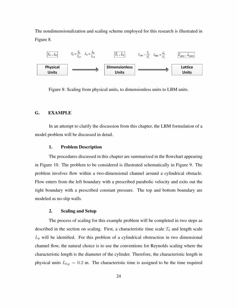
The nondimensionalization and scaling scheme employed for this research is illustrated in

Figure 8.

Figure 8: Scaling from physical units, to dimensionless units to LBM units.

G. EXAMPLE

In an attempt to clarify the discussion from this chapter, the LBM formulation of a

model problem will be discussed in detail.

1. Problem Description

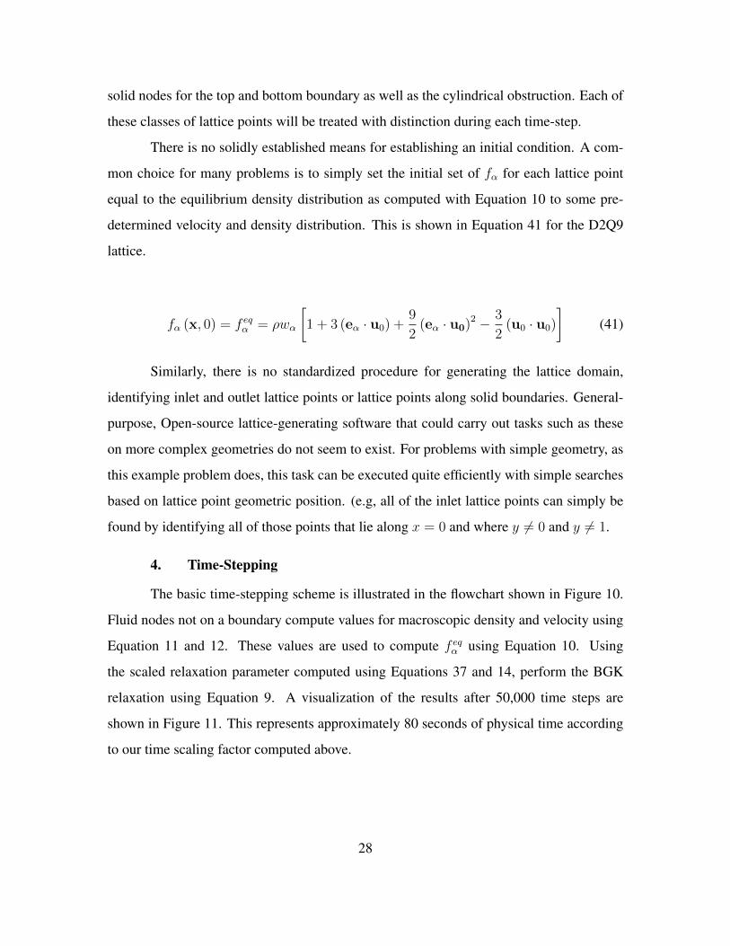
The procedures discussed in this chapter are summarized in the flowchart appearing

in Figure 10. The problem to be considered is illustrated schematically in Figure 9. The

problem involves flow within a two-dimensional channel around a cylindrical obstacle.

Flow enters from the left boundary with a prescribed parabolic velocity and exits out the

right boundary with a prescribed constant pressure. The top and bottom boundary are

modeled as no-slip walls.

2. Scaling and Setup

The process of scaling for this example problem will be completed in two steps as

described in the section on scaling. First, a characteristic time scale T0 and length scale

L0 will be identified. For this problem of a cylindrical obstruction in two dimensional

channel flow, the natural choice is to use the conventions for Reynolds scaling where the

characteristic length is the diameter of the cylinder. Therefore, the characteristic length in

physical units L0,p = 0.2 m. The characteristic time is assigned to be the time required

24

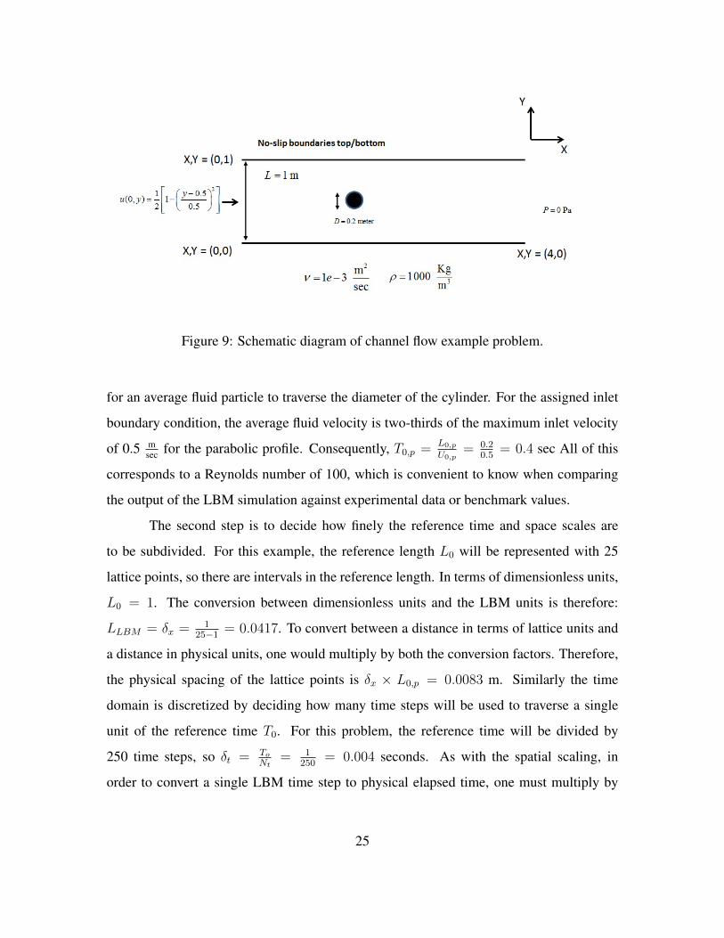
Figure 9: Schematic diagram of channel flow example problem.

for an average fluid particle to traverse the diameter of the cylinder. For the assigned inlet

boundary condition, the average fluid velocity is two-thirds of the maximum inlet velocity

of 0.5 msec for the parabolic profile. Consequently, T0,p = L0,p

U0,p= 0.2

0.5= 0.4 sec All of this

corresponds to a Reynolds number of 100, which is convenient to know when comparing

the output of the LBM simulation against experimental data or benchmark values.

The second step is to decide how finely the reference time and space scales are

to be subdivided. For this example, the reference length L0 will be represented with 25

lattice points, so there are intervals in the reference length. In terms of dimensionless units,

L0 = 1. The conversion between dimensionless units and the LBM units is therefore:

LLBM = δx = 125−1

= 0.0417. To convert between a distance in terms of lattice units and

a distance in physical units, one would multiply by both the conversion factors. Therefore,

the physical spacing of the lattice points is δx × L0,p = 0.0083 m. Similarly the time

domain is discretized by deciding how many time steps will be used to traverse a single

unit of the reference time T0. For this problem, the reference time will be divided by

250 time steps, so δt = ToNt

= 1250

= 0.004 seconds. As with the spatial scaling, in

order to convert a single LBM time step to physical elapsed time, one must multiply by

25

the scaling parameters between the Dimensionless units and LBM units in addition to the

conversion between Physical and Dimensionless units. For this problem, those conversions

are TP = TLBM × δt × T0 = 0.0016.

Once the spatial and temporal scaling factors are determined, the properly scaled

LBM parameters must be determined from the given physical data.

a. Viscosity Scaling

In order to get dynamic LBM behavior that corresponds to the desired phys-

ical fluid under the prescribed conditions, the temporal and spatial scaling factors need to

be applied to the specified fluid kinematic viscosity ν. Since ν has units of m2

sec the necessary

conversion can be accomplished via Equation 37.

νLBM = νPhysical ×T0δt

(L0δx)2 (37)

Carrying out this conversion for the specified fluid with the chosen dis-

cretization results in νLBM = 0.023. This is the value that is applied to Equation 14 to

find the LBM relaxation parameter. Doing so for this problem results in τ = 0.57 or

ω = 1.76

b. Velocity BC Scaling

This problem has a prescribed inlet velocity profile. The velocity is ex-

pressed in terms of meters-per-second, which is not compatible with the unit system as-

sumed when the LBM boundary conditions were developed. The velocity is simply scaled

in accordance with Equation 38.

uLBM = uPhysical ×T0δtL0δx

(38)

For this problem, this conversion reads:

u(0, y) =3

4

[1− (y − 0.5)

0.5

]× 0.0016

0.0083= 0.144

[1− (y − 0.5)

0.5

].

26

This is the velocity that will be passed to the LBM time-stepping routine in order to set the

prescribed velocity at the inlet lattice points.

c. Pressure BC Scaling

For this problem, the prescribed outlet pressure is set to 0 Pa. This is a

relative pressure, of course, otherwise the density for lattice points at the outlet would

need to be set to zero according to Equation 13. Since the prescribed pressure boundary

condition procedures are actually methods for enforcing a specific density at the boundary,

in order to employ the pressure boundary condition for evaluating pressure on the domain

we must:

• Compute the pressure through the domain using Equation 11 and Equation 13 along

with the value of cs applicable for the lattice in use.

• Scale the computed pressure to physical units using Equation 39. In this step, one is

simply converting c2s to physical units.

• Adjust the pressure in physical units so that the boundary condition is satisfied as in

Equation 40.

PPhysical = ρLBMc2s

(δxL0

δtT0

)2

(39)

P = PPhysical − PBoundary (40)

3. Initialization and Lattice Point Classification

As final steps before commencing the LBM time-stepping routine, the initial values

for fα must be established for all lattice points. Additionally, all boundary lattice points,

solid lattice points, and any other type of lattice point that will require special treatment

must be identified. For this problem, we need only identify inlet nodes for the prescribed

velocity boundary condition, outlet nodes for the pressure boundary condition as well as

27

solid nodes for the top and bottom boundary as well as the cylindrical obstruction. Each of

these classes of lattice points will be treated with distinction during each time-step.

There is no solidly established means for establishing an initial condition. A com-

mon choice for many problems is to simply set the initial set of fα for each lattice point

equal to the equilibrium density distribution as computed with Equation 10 to some pre-

determined velocity and density distribution. This is shown in Equation 41 for the D2Q9

lattice.

fα (x, 0) = f eqα = ρwα

[1 + 3 (eα · u0) +

9

2(eα · u0)2 − 3

2(u0 · u0)

](41)

Similarly, there is no standardized procedure for generating the lattice domain,

identifying inlet and outlet lattice points or lattice points along solid boundaries. General-

purpose, Open-source lattice-generating software that could carry out tasks such as these

on more complex geometries do not seem to exist. For problems with simple geometry, as

this example problem does, this task can be executed quite efficiently with simple searches

based on lattice point geometric position. (e.g, all of the inlet lattice points can simply be

found by identifying all of those points that lie along x = 0 and where y 6= 0 and y 6= 1.

4. Time-Stepping

The basic time-stepping scheme is illustrated in the flowchart shown in Figure 10.

Fluid nodes not on a boundary compute values for macroscopic density and velocity using

Equation 11 and 12. These values are used to compute f eqα using Equation 10. Using

the scaled relaxation parameter computed using Equations 37 and 14, perform the BGK

relaxation using Equation 9. A visualization of the results after 50,000 time steps are

shown in Figure 11. This represents approximately 80 seconds of physical time according

to our time scaling factor computed above.

28

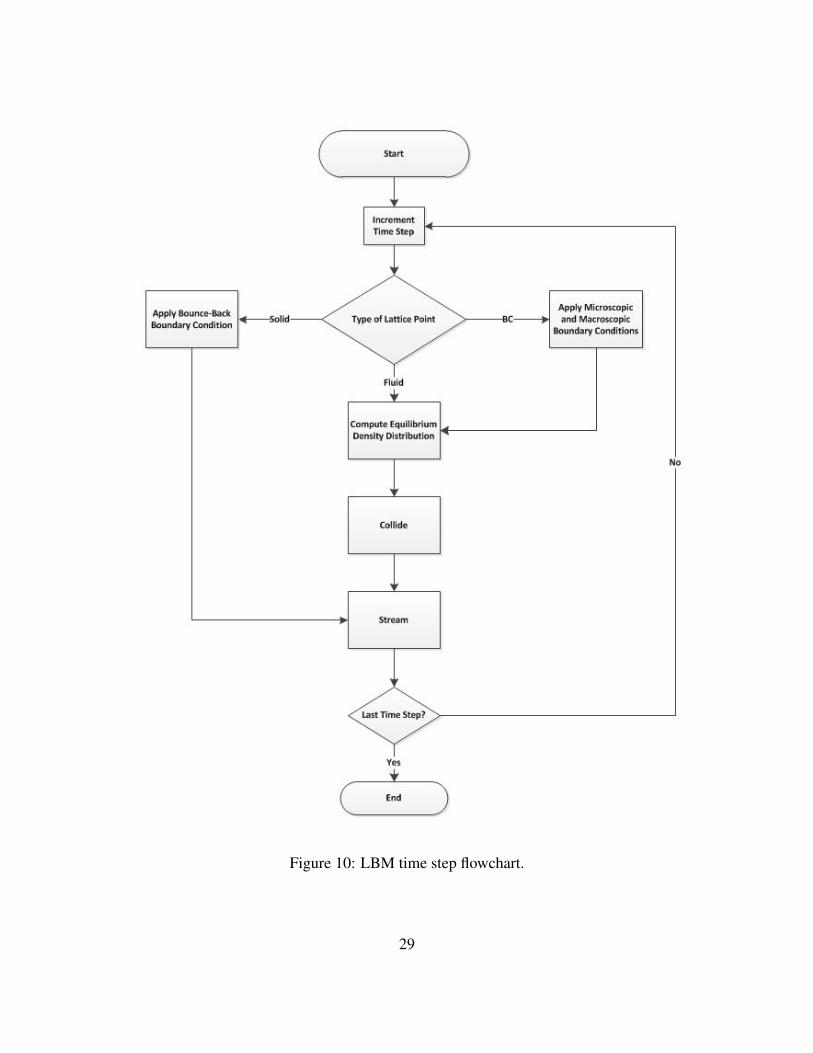
Figure 10: LBM time step flowchart.

29

AA>IY 8ounu-Bo<k l•4t-~5olof,fdl---< Bound"'Y Condition

Start

Type of Lattioe Point

Huid

Apply Mkroscop;c and Mac:roscopic

llou~IY Conditions

Compute Equilibrium 1.-----------__J Oonslty Distribution

Collide

y.,

* (~_End~)

No

Figure 11: Velocity magnitude, pressure, and vorticity magnitude for example flow caseafter 50,000 time steps.

30

III. IMPLEMENTATION AND VALIDATION

In order to model fluid structure interactions with LBM and FEM, it is necessary

to have available a reliable, flexible and powerful implementation of the LBM. It must

first be reliable so that we can have some reasonable hope that the results obtained will be

comparable to physical reality. It must be flexible so that a wide variety of simulations can

be conducted, pertaining to different physical conditions of interest. It must be powerful so

that these simulations can be refined for greater accuracy while still able to be completed

in a reasonable amount of time.

In this chapter, a body of software tools, designed using the theory presented in

Chapter II, is tested against a selection of standard benchmarks first for accuracy and then

for performance. The following results are obtained from this work:

• The LBM software as implemented for this work reliably reproduces re-

sults obtained Poiseuille flow, lid-driven cavity, flow over a backward step

and flow over a cylindrical obstruction for 2D.

• The LBM provides second-order convergence to the 2D Poiseuille flow

with appropriate boundary conditions and double precision arithmetic. A

mixed-precision algorithm is introduced which allows similar second-order

convergence while only storing single-precision data.

• The LBM is benchmarked for performance against recently published im-

plementations for 3D lid-driven cavity flow. It is shown that the software

produced for this work has competitive performance with other single-

workstation implementations recently produced.

A. POISEUILLE FLOW

The first test case is a two-dimensional flow case between parallel plates. The flow

condition is depicted in Figure 12.

31

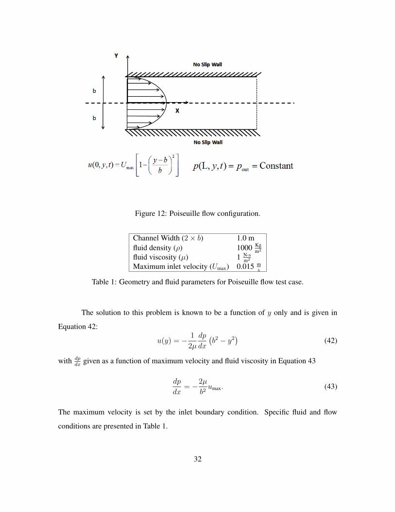
Figure 12: Poiseuille flow configuration.

Channel Width (2× b) 1.0 mfluid density (ρ) 1000 Kg

m2

fluid viscosity (µ) 1 N-sm2

Maximum inlet velocity (Umax) 0.015 ms

Table 1: Geometry and fluid parameters for Poiseuille flow test case.

The solution to this problem is known to be a function of y only and is given in

Equation 42:

u(y) = − 1

2µ

dp

dx

(b2 − y2

)(42)

with dpdx

given as a function of maximum velocity and fluid viscosity in Equation 43

dp

dx= −2µ

b2umax. (43)

The maximum velocity is set by the inlet boundary condition. Specific fluid and flow

conditions are presented in Table 1.

32

1. Solution with On-Grid Bounceback Boundary Conditions

For the LBM model of this problem, the D2Q9 lattice with LBGK dynamics was

used along with Zou/He boundary conditions for the prescribed velocity on the west bound-

ary and constant prescribed pressure on the east boundary. The initial lattice discretization

was set so that 30 lattice points would span the channel entrance. The time step was set to

achieve a relaxation parameter ω of 1.30. While refining the grid to test for convergence,

the time step was adjusted so as to maintain a constant relaxation parameter for all tests.

The results are shown in Figure 13. As expected, first-order convergence is obtained for

this style of boundary condition.

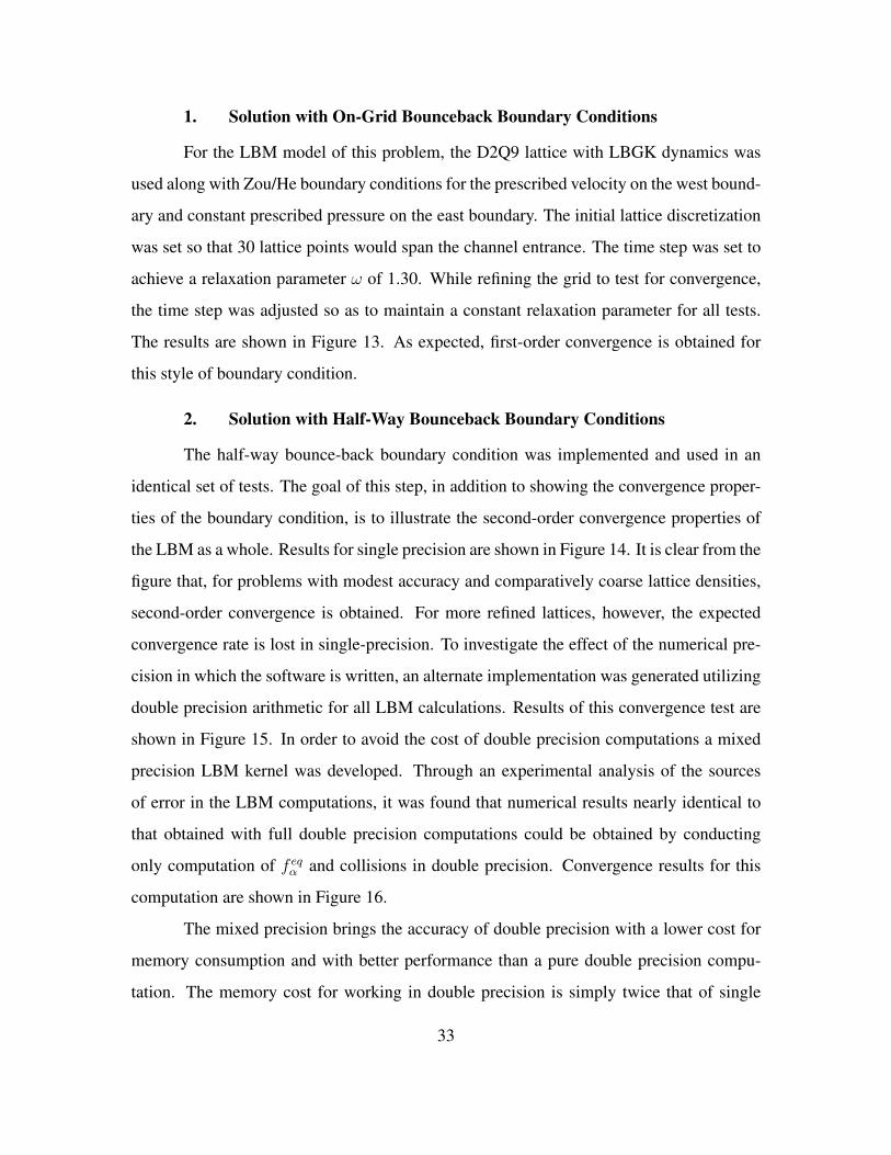
2. Solution with Half-Way Bounceback Boundary Conditions

The half-way bounce-back boundary condition was implemented and used in an

identical set of tests. The goal of this step, in addition to showing the convergence proper-

ties of the boundary condition, is to illustrate the second-order convergence properties of

the LBM as a whole. Results for single precision are shown in Figure 14. It is clear from the

figure that, for problems with modest accuracy and comparatively coarse lattice densities,

second-order convergence is obtained. For more refined lattices, however, the expected

convergence rate is lost in single-precision. To investigate the effect of the numerical pre-

cision in which the software is written, an alternate implementation was generated utilizing

double precision arithmetic for all LBM calculations. Results of this convergence test are

shown in Figure 15. In order to avoid the cost of double precision computations a mixed

precision LBM kernel was developed. Through an experimental analysis of the sources

of error in the LBM computations, it was found that numerical results nearly identical to

that obtained with full double precision computations could be obtained by conducting

only computation of f eqα and collisions in double precision. Convergence results for this

computation are shown in Figure 16.

The mixed precision brings the accuracy of double precision with a lower cost for

memory consumption and with better performance than a pure double precision compu-

tation. The memory cost for working in double precision is simply twice that of single

33

Figure 13: Poiseuille flow convergence with On-Grid bounce-back boundary conditions.

34

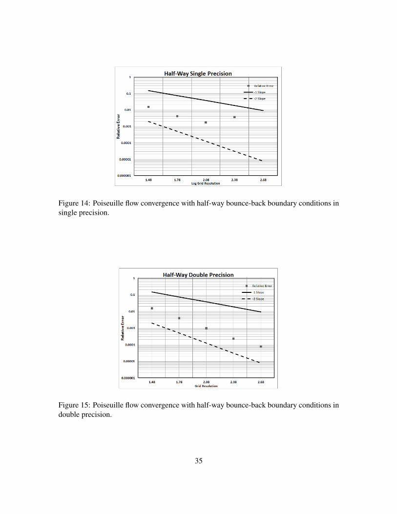
Figure 14: Poiseuille flow convergence with half-way bounce-back boundary conditions insingle precision.

Figure 15: Poiseuille flow convergence with half-way bounce-back boundary conditions indouble precision.

35

Figure 16: Poiseuille flow convergence with half-way bounce-back boundary conditionsusing mixed-precision arithmetic.

precision. The relative computational performance of single, mixed and double precision

are presented in Figure 17 for two-dimensional Poiseuille flow using the LBGK collision

operator. For less refined lattices, the double precision performance is nearly identical to

single precision and both are slightly higher than mixed precision. For more dense lattices

the additional memory-bandwidth load of passing double precision operands to the com-

putational routines becomes more important than penalties paid for type conversions and

mixed precision outperforms double precision.

3. Stability and Accuracy

In the preceding section, it may have seemed arbitrary to have selected a constant

relaxation parameter ω = 1.25. This conclusion is partially correct insofar as there is

considerable flexibility as to how this value is picked. We recall from Chapter II that,

including effects of scaling in time and space, the fluid viscosity in LBM-units scales by δtδ2x

in accordance with Equation 37. Consequently, if δx is reduced by a factor of 2, δt must be

reduced by a factor of 4. With this refined time step, the number of time steps is increased

by a factor of 4 for the fluid simulation, including the time required for the LBM simulation

36

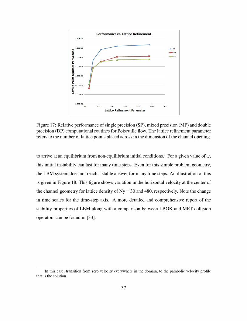
Figure 17: Relative performance of single precision (SP), mixed precision (MP) and doubleprecision (DP) computational routines for Poiseuille flow. The lattice refinement parameterrefers to the number of lattice points placed across in the dimension of the channel opening.

to arrive at an equilibrium from non-equilibrium initial conditions.1 For a given value of ω,

this initial instability can last for many time steps. Even for this simple problem geometry,

the LBM system does not reach a stable answer for many time steps. An illustration of this

is given in Figure 18. This figure shows variation in the horizontal velocity at the center of

the channel geometry for lattice density of Ny = 30 and 480, respectively. Note the change

in time scales for the time-step axis. A more detailed and comprehensive report of the

stability properties of LBM along with a comparison between LBGK and MRT collision

operators can be found in [33].

1In this case, transition from zero velocity everywhere in the domain, to the parabolic velocity profilethat is the solution.

37

Figure 18: Stabilization time for Poiseuille flow, Re=10, 1τ

= ω = 1.3. Top figure, Ny=30,bottom figure, Ny=480.

38

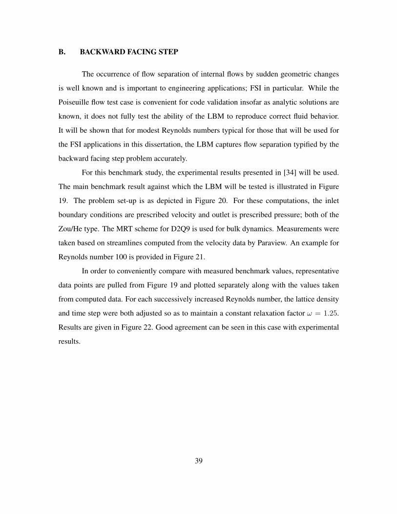
B. BACKWARD FACING STEP

The occurrence of flow separation of internal flows by sudden geometric changes

is well known and is important to engineering applications; FSI in particular. While the

Poiseuille flow test case is convenient for code validation insofar as analytic solutions are

known, it does not fully test the ability of the LBM to reproduce correct fluid behavior.

It will be shown that for modest Reynolds numbers typical for those that will be used for

the FSI applications in this dissertation, the LBM captures flow separation typified by the

backward facing step problem accurately.

For this benchmark study, the experimental results presented in [34] will be used.

The main benchmark result against which the LBM will be tested is illustrated in Figure

19. The problem set-up is as depicted in Figure 20. For these computations, the inlet

boundary conditions are prescribed velocity and outlet is prescribed pressure; both of the

Zou/He type. The MRT scheme for D2Q9 is used for bulk dynamics. Measurements were

taken based on streamlines computed from the velocity data by Paraview. An example for

Reynolds number 100 is provided in Figure 21.

In order to conveniently compare with measured benchmark values, representative

data points are pulled from Figure 19 and plotted separately along with the values taken

from computed data. For each successively increased Reynolds number, the lattice density

and time step were both adjusted so as to maintain a constant relaxation factor ω = 1.25.

Results are given in Figure 22. Good agreement can be seen in this case with experimental

results.

39

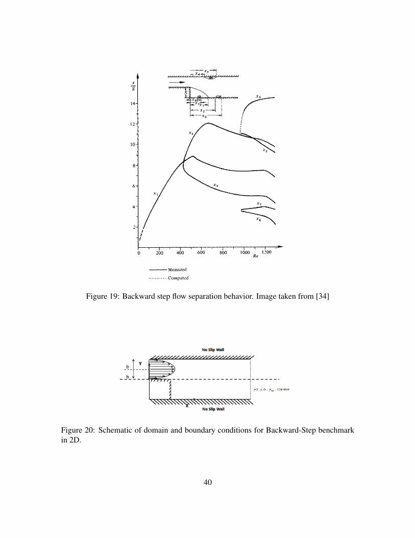
Figure 19: Backward step flow separation behavior. Image taken from [34]

Figure 20: Schematic of domain and boundary conditions for Backward-Step benchmarkin 2D.

40

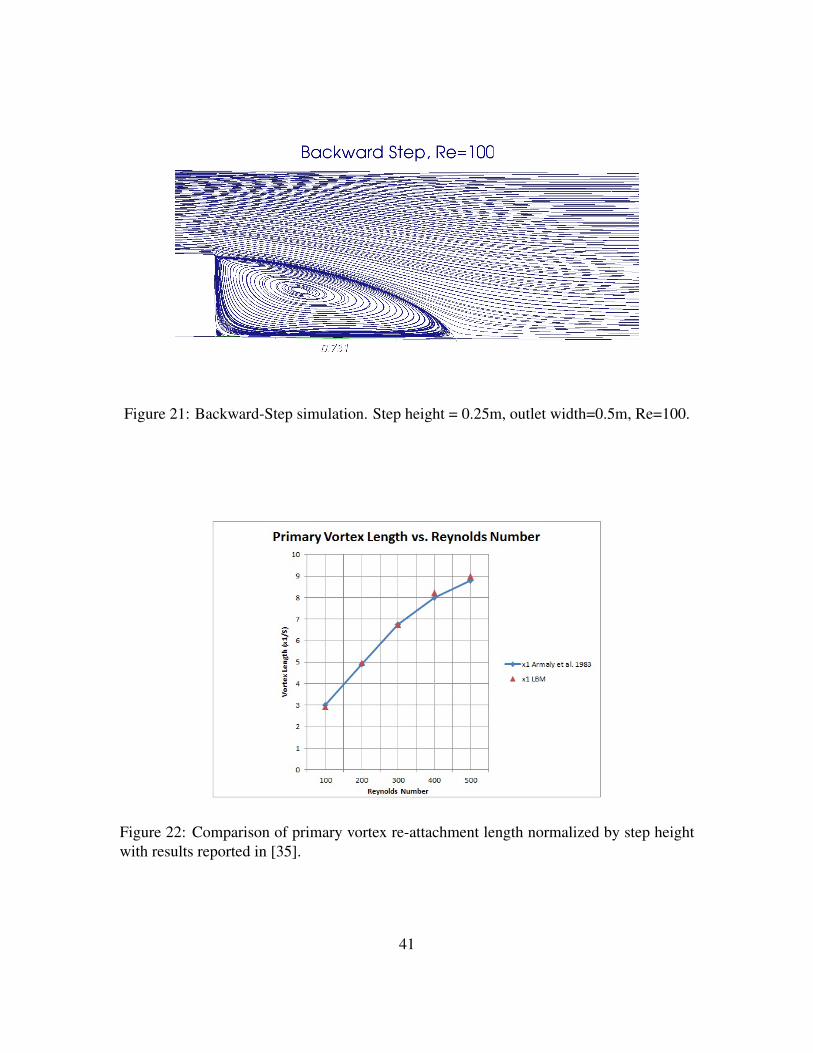
Figure 21: Backward-Step simulation. Step height = 0.25m, outlet width=0.5m, Re=100.

Figure 22: Comparison of primary vortex re-attachment length normalized by step heightwith results reported in [35].

41

C. LID-DRIVEN CAVITY

As one validation of the LBM implementation, the software was used to simulate

lid-driven flow in two dimensions. A commonly used benchmark for this flow condition is

given in [35]. A schematic illustration of the two-dimensional lid-driven cavity problem is

given in Figure 23.

Figure 23: Schematic of the two-dimensional lid-driven cavity problem.

Boundary conditions used for this project are on-grid bounce-back to model no-slip

stationary walls. The moving-wall boundary condition is used to model the lid. The lid

velocity is set to a constant value in the x direction with the desired speed. The standard

benchmark stipulates a Reynolds number of 1000, though other authors have published

results at higher Re. In two dimensions, the D2Q9 lattice is used with either LBGK or

MRT bulk dynamics.

In Figure 24, a qualitative comparison is made with results reported in [36]. In Fig-

ure 25, a qualitative comparison is made of the streamlines, pressure contours and vorticity

contours with those published in [37]. Quantitative comparisons are made in the following

figures.

42

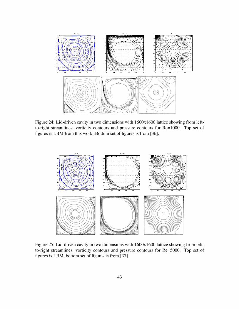
Figure 24: Lid-driven cavity in two dimensions with 1600x1600 lattice showing from left-to-right streamlines, vorticity contours and pressure contours for Re=1000. Top set offigures is LBM from this work. Bottom set of figures is from [36].

Figure 25: Lid-driven cavity in two dimensions with 1600x1600 lattice showing from left-to-right streamlines, vorticity contours and pressure contours for Re=5000. Top set offigures is LBM, bottom set of figures is from [37].

43

In Figure 26, two samples of velocity are taken in the computed problem domain.

The first is the x velocity component sampled along the vertical center-line. As can be seen,

good agreement with benchmark values is obtained for all macroscopic fluid parameters.

44

Figure 26: Comparison of velocity, pressure and vorticity to benchmark values forRe=1000.

45

D. CHANNEL FLOW OVER CYLINDER

The flow configuration for this benchmark is illustrated in Figure 27. Constant

velocity is specified on the inlet and constant pressure is specified on the outlet. The top

and bottom of the domain are simulated as periodic boundaries with the result that the

effective domain is a linear array of cylinders in uniform flow. Similar work cited for the

benchmarks are published in [38]-[44]. The trailing vortex region for this benchmark was

measured visually following flow simulation. Numeric results are given in Table 2 and

graphically in Figure 28. It can be seen from the table that the computed values using LBM

are comparable to those reported in the literature.

Figure 27: Channel with cylindrical obstacle 2D problem.

Author Re = 20 Re = 40Zhou (2012) 0.92 2.20Calhoun (2002) 0.91 2.18Rusell (2003) 0.94 2.35Silva (2003) 1.04 2.55This work 0.95 2.05

Table 2: Comparison of trailing vortex length to benchmark values.

46

Figure 28: Streamline visualization of trailing vortex at Re=20 (top) and Re=40 (bottom).

Above a Reynolds number of approximately 45, the trailing vortex detaches in an

alternating pattern referred to as a Von Karman street. As a last measure, the rate of vortex

shedding was measured and the non-dimensional Strouhal number was evaluated with the

result compared to the literature. A visualization of the vorticity in the wake of a circular

cylinder in channel flow at Reynolds number of 100 is given in Figure 29. Notice the

alternating regions of positive and negative vorticity resulting from the vortex shedding

alternately from the top and bottom of the cylinder. The equation for the Strouhal number

is given in Equation 44,

St =fL0

U0

(44)

where St is the non-dimensional Strouhal number, f is the frequency of vortex shedding,

L0 is the characteristic length and U0 is the characteristic velocity. For this problem, the

characteristic length is the diameter of the cylinder and the characteristic velocity is the

47

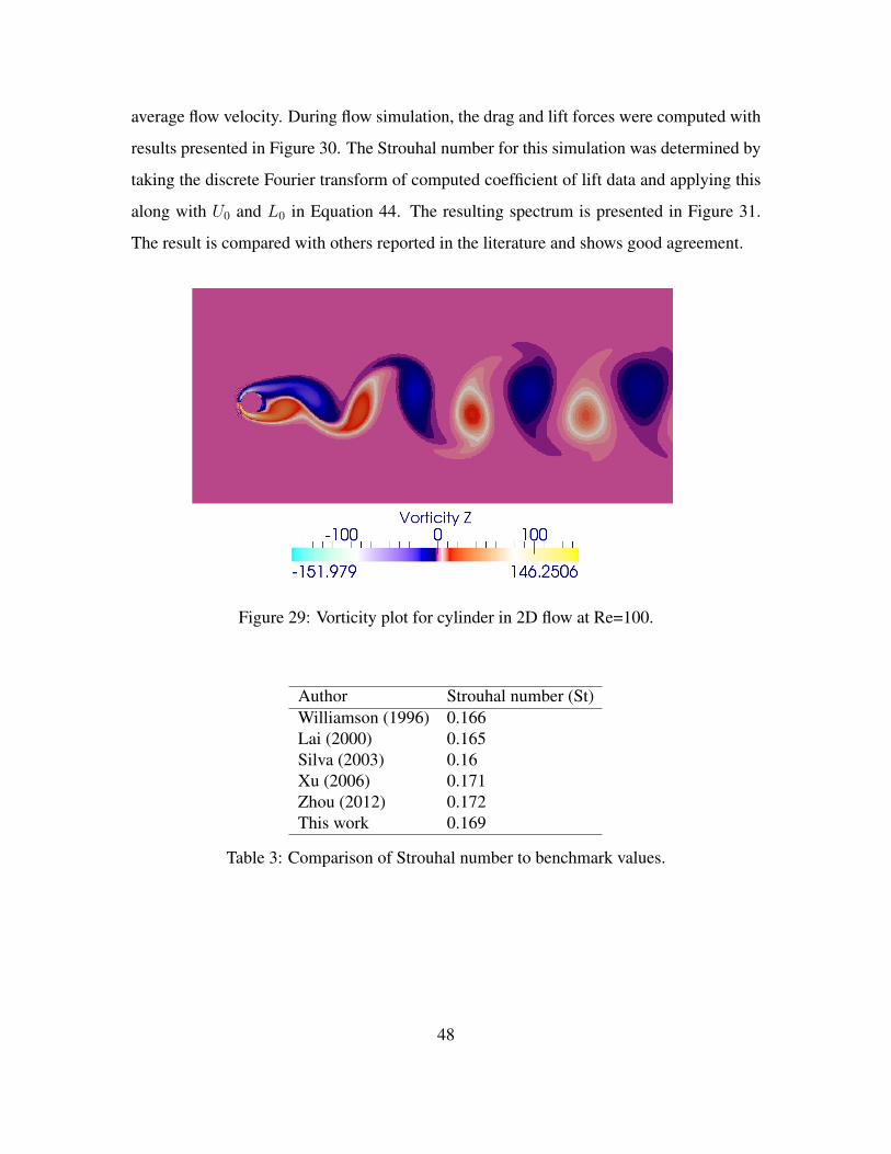
average flow velocity. During flow simulation, the drag and lift forces were computed with

results presented in Figure 30. The Strouhal number for this simulation was determined by

taking the discrete Fourier transform of computed coefficient of lift data and applying this

along with U0 and L0 in Equation 44. The resulting spectrum is presented in Figure 31.

The result is compared with others reported in the literature and shows good agreement.

Figure 29: Vorticity plot for cylinder in 2D flow at Re=100.

Author Strouhal number (St)Williamson (1996) 0.166Lai (2000) 0.165Silva (2003) 0.16Xu (2006) 0.171Zhou (2012) 0.172This work 0.169

Table 3: Comparison of Strouhal number to benchmark values.

48

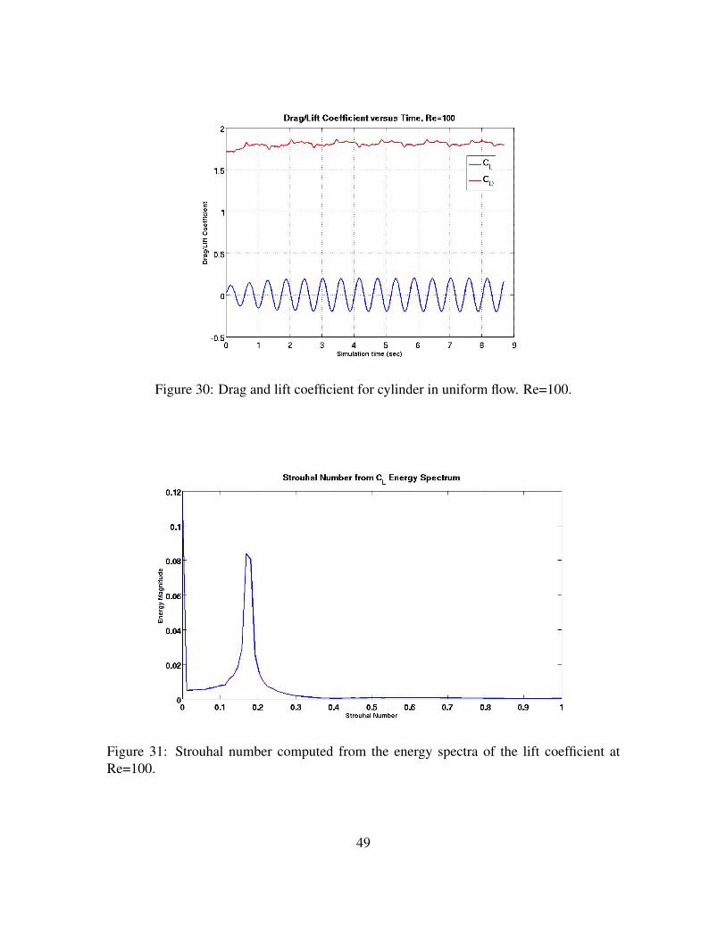
Figure 30: Drag and lift coefficient for cylinder in uniform flow. Re=100.

Figure 31: Strouhal number computed from the energy spectra of the lift coefficient atRe=100.

49


50

IV. LBM IMPLEMENTATION ON GRAPHICS PROCESSINGUNITS

With recent advances in modern GPUs the interest in using these devices for sci-

entific calculations has been growing. In particular, the memory-bandwidth and compute

capability of GPUs compared to contemporary CPUs has made their use for LBM ap-

plications particularly appealing. Implementations of the LBM using CUDA and the C

programming language have been published and the viability of the GPU as an effective

platform for executing the LBM has been demonstrated extensively [45]-[50].

In this chapter, the computational requirements for the LBM will be reviewed. Next

the NVIDIA CUDA GPU computing platform is introduced and its use for the LBM sim-

ulations presented in this work is outlined. Comparisons are made to recently published

performance benchmarks for systems with a single GPU. Lastly, multi-GPU implementa-

tions of the LBM in hybrid parallel schemes employing CUDA with OpenMP as well as

CUDA with MPI will be presented. Performance of these codes are compared with a more

conventional parallel implementation with MPI.

A. COMPUTATIONAL REQUIREMENTS FOR THE LBM

Though the operations to be executed for each lattice point during each time step are

conceptually straightforward and easy to implement on a computer, it has been well recog-

nized in the literature that the LBM is particularly computationally intensive and memory

demanding [51]. Considerations for precision and stability combine to dictate a require-

ment that a large number of lattice points are needed to effectively discretize a problem

domain. Within the classical LBM formulation, all lattice points must be equally spaced

implying that LBM solutions for problems with widely varying length and time scales of

interest would perform worse than an equivalent finite element method (FEM) or finite

volume method (FVM) code where non-uniform meshes may be used. In addition to the

large number of lattice points, each lattice point in the domain requires storage for each

51

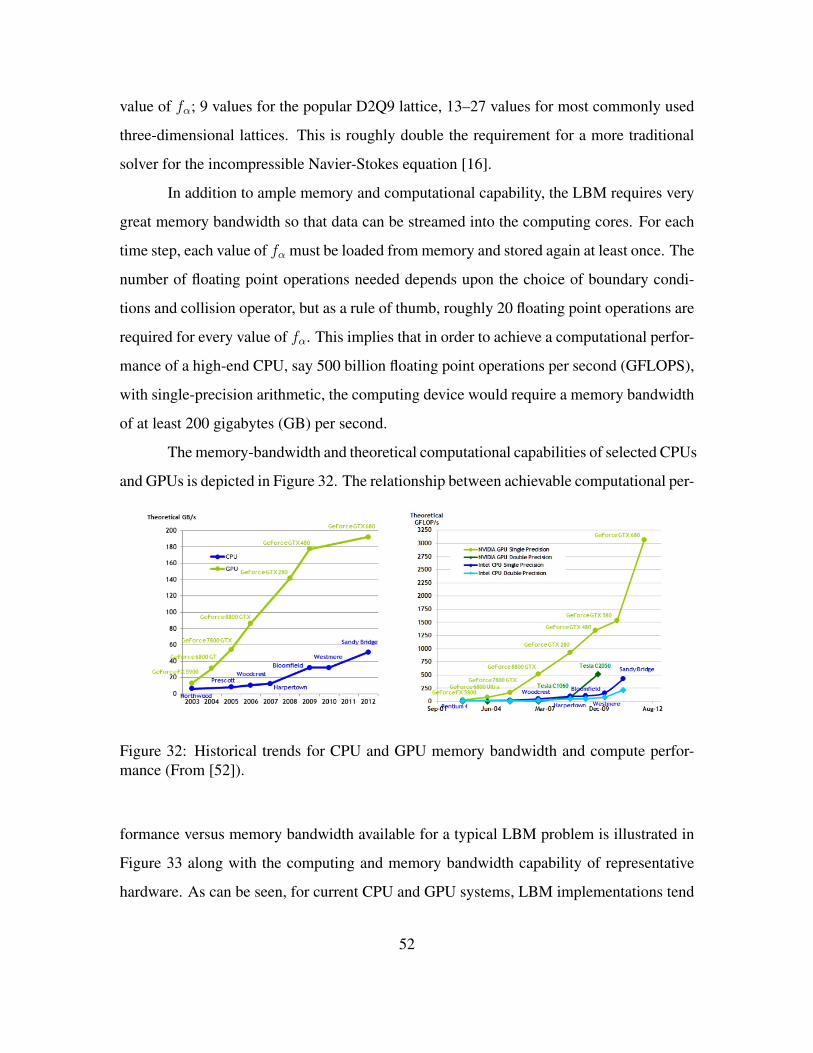
value of fα; 9 values for the popular D2Q9 lattice, 13–27 values for most commonly used

three-dimensional lattices. This is roughly double the requirement for a more traditional

solver for the incompressible Navier-Stokes equation [16].

In addition to ample memory and computational capability, the LBM requires very

great memory bandwidth so that data can be streamed into the computing cores. For each

time step, each value of fα must be loaded from memory and stored again at least once. The

number of floating point operations needed depends upon the choice of boundary condi-

tions and collision operator, but as a rule of thumb, roughly 20 floating point operations are

required for every value of fα. This implies that in order to achieve a computational perfor-

mance of a high-end CPU, say 500 billion floating point operations per second (GFLOPS),

with single-precision arithmetic, the computing device would require a memory bandwidth

of at least 200 gigabytes (GB) per second.

The memory-bandwidth and theoretical computational capabilities of selected CPUs

and GPUs is depicted in Figure 32. The relationship between achievable computational per-

Figure 32: Historical trends for CPU and GPU memory bandwidth and compute perfor-mance (From [52]).

formance versus memory bandwidth available for a typical LBM problem is illustrated in

Figure 33 along with the computing and memory bandwidth capability of representative

hardware. As can be seen, for current CPU and GPU systems, LBM implementations tend

52

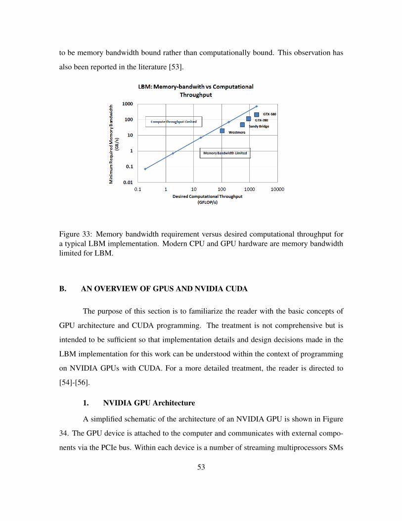
to be memory bandwidth bound rather than computationally bound. This observation has

also been reported in the literature [53].

Figure 33: Memory bandwidth requirement versus desired computational throughput fora typical LBM implementation. Modern CPU and GPU hardware are memory bandwidthlimited for LBM.

B. AN OVERVIEW OF GPUS AND NVIDIA CUDA

The purpose of this section is to familiarize the reader with the basic concepts of

GPU architecture and CUDA programming. The treatment is not comprehensive but is

intended to be sufficient so that implementation details and design decisions made in the

LBM implementation for this work can be understood within the context of programming

on NVIDIA GPUs with CUDA. For a more detailed treatment, the reader is directed to

[54]-[56].

1. NVIDIA GPU Architecture

A simplified schematic of the architecture of an NVIDIA GPU is shown in Figure

34. The GPU device is attached to the computer and communicates with external compo-

nents via the PCIe bus. Within each device is a number of streaming multiprocessors SMs

53

and within each SM is a number of scalar processors (SPs). The number of SMs per device

and the number of SPs per SM varies between generations of GPUs and among particular

models in a given generation. Each SM contains a register file used by the SPs as well as

a memory space that serves partly as a level 1 cache and a user-managed shared memory.

The device also contains a bank of level 2 cache as well as a bank of device memory that

is characterized by greater capacity but slower access.

Figure 34: Simplified schematic of NVIDIA GPU.

The NVIDIA GPU is designed for highly multithreaded high-throughput comput-

ing. Each scalar processor is assigned a thread for execution. Threads are organized in a

hierarchical way into blocks and grids as illustrated by Figure 35. Multithreaded programs

executing on the GPU are “launched” as a grid of thread blocks. Grids of threads are com-

posed of at three dimensional array of blocks. The blocks, in turn, are composed of a three

dimensional array of threads. The blocks are distributed among the SMs for execution.

Each of the SMs execute the threads contained within each thread block independently

54

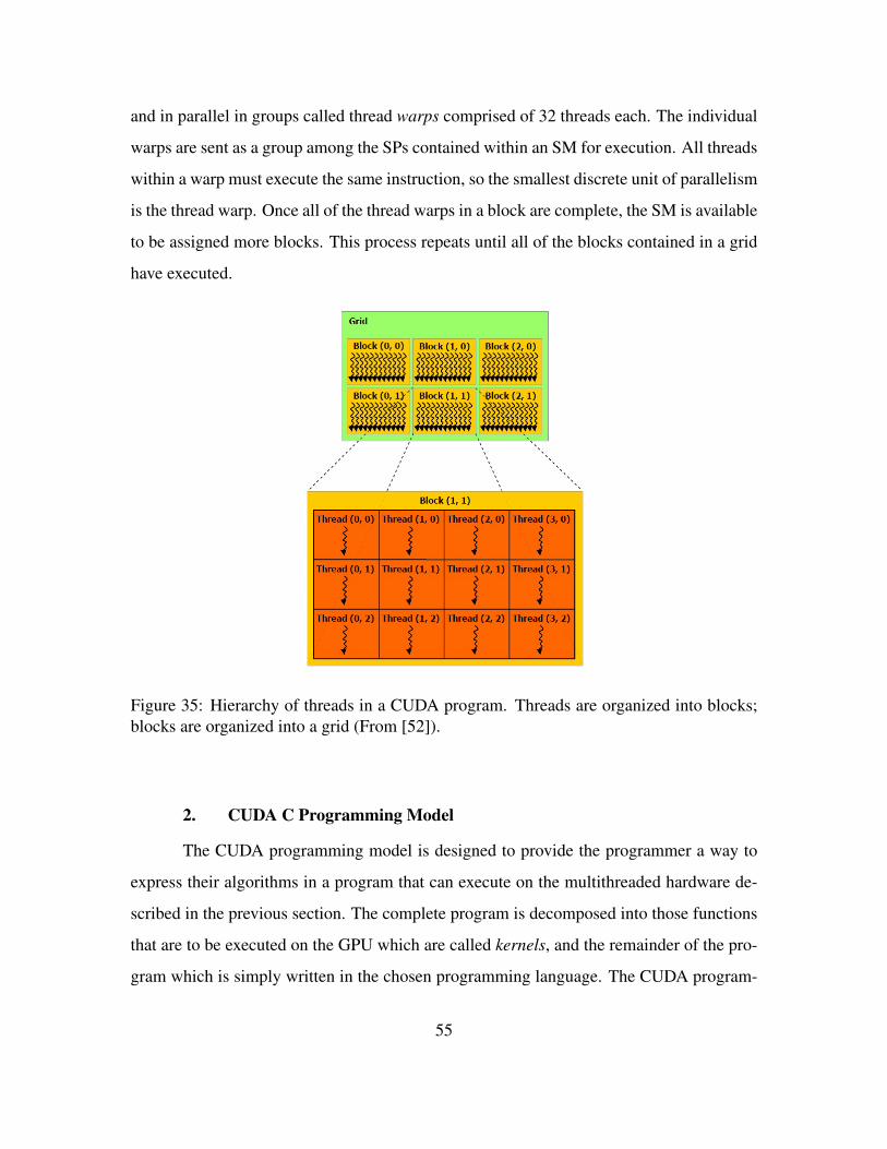
and in parallel in groups called thread warps comprised of 32 threads each. The individual

warps are sent as a group among the SPs contained within an SM for execution. All threads

within a warp must execute the same instruction, so the smallest discrete unit of parallelism

is the thread warp. Once all of the thread warps in a block are complete, the SM is available

to be assigned more blocks. This process repeats until all of the blocks contained in a grid

have executed.

Figure 35: Hierarchy of threads in a CUDA program. Threads are organized into blocks;blocks are organized into a grid (From [52]).

2. CUDA C Programming Model

The CUDA programming model is designed to provide the programmer a way to

express their algorithms in a program that can execute on the multithreaded hardware de-

scribed in the previous section. The complete program is decomposed into those functions

that are to be executed on the GPU which are called kernels, and the remainder of the pro-

gram which is simply written in the chosen programming language. The CUDA program-

55

ming model augments the C programming language with additional syntax and keywords

along with an extensive application programming interface (API) enabling the programmer

to to effect common programming tasks targeted for the GPU such as device selection,

memory allocation, memory transfer and memory de-allocation. Functions that are written

for execution on the GPU are denoted with the global qualifier as illustrated in the code

listing below.

Within the C source code, the kernels are invoked with a special syntax in which the pro-

grammer specifies the dimensions of the grid (i.e., configuration of block array within the

grid and configuration of the thread array within each block). The syntax is illustrated in

the code listing below:

where dim3 is an integer vector defined as part of the CUDA API that is used to express

the grid and block dimensions.

From the programmer’s perspective, scaling of thread execution among SMs and

SPs is transparent. It is not even necessary for the programmer to be aware of how many

SMs or SPs are present in a system. Code written for one GPU with a given number of

SMs and SPs will run without modification or even recompilation on a GPU with twice as

many of each; it will just run faster.

Some restrictions exist in the CUDA programming model. The programmer has

no control over the order in which the thread blocks will execute. Additionally, no global

thread synchronization within the context of a single kernel is possible. Once started each

thread block runs to completion; the programmer can only enforce barrier synchronization

for threads within an individual thread block.

56

Like other shared-memory programming models such as OpenMP, CUDA does

facilitate shared variables between individual threads. For CUDA, this is only possible for

threads within a single thread block. This is done using the shared memory block within

each SM. Any data that must be exchanged with threads outside of the thread block must be

done via global memory and, since execution of distinct thread blocks cannot be scheduled

by the programmer, it must be done asynchronously.

A programmer planning to use CUDA to obtain high performance must design their

programs so as to make maximum use of computing resources while not overloading the

available memory bandwidth. Maximizing use of the computing resources means mapping

the most fine-grained level of parallelism within the algorithm to the grid structure provided

in the CUDA programming model to generate as many threads as possible. Using LBM as

an example the choice almost universally made is to assign all of the computations required

for a single lattice point to a unique CUDA thread. All of the threads for all of the lattice

points would then be mapped into blocks and ultimately a thread grid for execution. For

simulations with many lattice points, this will generate sufficient parallelism to keep many

of the SMs and their associated SPs busy doing productive work.

Conservation of global memory bandwidth is done in two ways: first, by minimiz-

ing the number of global memory transactions; second, by ensuring that the global mem-

ory transactions are as efficient as possible by ensuring load and store operations to global

memory are coalesced. For GPU programming of the LBM, there is much less agreement

in how best to achieve the goal of making best use of available memory resources. This is

not surprising since efficient use of memory bandwidth is the most important determiner of

program performance. Some of the design alternatives will be discussed in the section on

LBM implementation with CUDA.

A great deal of effort is made among researchers to ensure that their programs

make the most effective use possible of their GPUs. The resulting codes and algorithms are

somewhat more complex than what will be described in this work. Instead of employing

every last arcane trick to squeeze the last epsilon of efficiency from the GPU, this work

57

will demonstrate the effectiveness of straight-forward though efficiently written code that

seeks first to embody the most important GPU programming best practices. A collection of

these high-level CUDA programming best practices is provided by NVIDIA in [57]. Some

of these guidelines are repeated here:

1. Minimize data transfer between the host and the device. Data transfer

should be avoided even if it means running some kernels on the device

even when they do not show significant performance gains compared to

running those functions on the CPU.

2. Ensure global memory accesses are coalesced whenever possible. Se-

quences of threads in a warp should, whenever possible, access sequential

locations of memory. When this is done the reading/writing operations can

be done in a single memory access.

3. Minimize the use of global memory. Prefer shared memory access where

possible.

4. Avoid different execution paths within the same warp. Use of if-then-

else control structures result in the requirement for warps to traverse code

segments multiple times as threads within the warp take different control

paths. This is termed thread divergence.

C. LBM IMPLEMENTATION WITH CUDA

In this section, the implementation strategy employed for this work will be outlined.

A great deal of software was written for this work, mainly comprising the multitude of

experiments in data layouts, grid setups and register usage strategies aimed at obtaining

high performance while maintaining some modicum of code flexibility. In the following

sections, both the basic implementation as well as steps taken towards optimization will be

reviewed in turn.

58

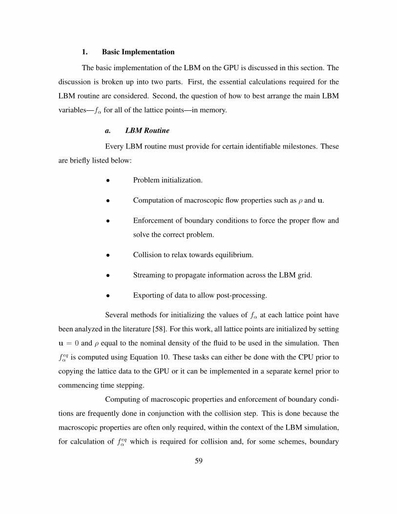
1. Basic Implementation

The basic implementation of the LBM on the GPU is discussed in this section. The

discussion is broken up into two parts. First, the essential calculations required for the

LBM routine are considered. Second, the question of how to best arrange the main LBM

variables—fα for all of the lattice points—in memory.

a. LBM Routine

Every LBM routine must provide for certain identifiable milestones. These

are briefly listed below:

• Problem initialization.

• Computation of macroscopic flow properties such as ρ and u.

• Enforcement of boundary conditions to force the proper flow and

solve the correct problem.

• Collision to relax towards equilibrium.

• Streaming to propagate information across the LBM grid.

• Exporting of data to allow post-processing.

Several methods for initializing the values of fα at each lattice point have

been analyzed in the literature [58]. For this work, all lattice points are initialized by setting

u = 0 and ρ equal to the nominal density of the fluid to be used in the simulation. Then

f eqα is computed using Equation 10. These tasks can either be done with the CPU prior to

copying the lattice data to the GPU or it can be implemented in a separate kernel prior to

commencing time stepping.

Computing of macroscopic properties and enforcement of boundary condi-

tions are frequently done in conjunction with the collision step. This is done because the

macroscopic properties are often only required, within the context of the LBM simulation,

for calculation of f eqα which is required for collision and, for some schemes, boundary

59

condition enforcement. To compute macroscopic properties separate from either boundary

condition enforcement or collision would require storing the values in global GPU memory.

For this reason, in light of the CUDA programming guidance to minimize global memory

transactions, the steps of computing macroscopic flow properties, boundary condition en-

forcement and collision are always done in the same kernel.

The streaming step for the classical LBM is simply a data copy operation.

While this is simple to implement, it is the subject of much research as to how to best

execute the streaming step in a way that memory accesses are coalesced.

Lastly, any simulation is pointless if there is no way to evaluate the results.

For this work, intermediate values for the fluid velocity and pressure field were periodically

transferred from the GPU to CPU and written to disk using Visualization Toolkit (VTK) file

formats. For FSI computations, displacement, velocity and acceleration data was similarly

stored for later post-processing.

b. Data Layout

The two principal alternative data layouts for LBM computations are the

so-called AoS or SoA. The two alternatives are illustrated schematically in Figure 36. In

AoS, the density distribution values fα for a given lattice point are assigned in consecutive

memory locations. In SoA, the density distribution for all of the lattice points for a given

lattice speed are assigned consecutive memory locations; these are followed by the density

distribution function for the next velocity and so-on until all of the data has a location.

For LBM calculations conducted on the CPU, it is most appealing use the

AoS since this will allow the CPU to access sequential memory locations while accessing

the data for a particular lattice point. This will allow for efficient memory transfers as well

as effective use of the memory cache hierarchy. In contrast, most LBM implementations

on the GPU use the SoA approach. With the SoA, when data is loaded from memory

within a kernel, each thread in a given warp reads from consecutive memory locations as

illustrated in Figure 37. When loads are coalesced in this fashion, the data is transferred

from memory in a single transaction. A similar condition exists during store operations as

60

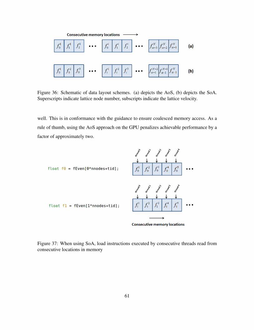
Figure 36: Schematic of data layout schemes. (a) depicts the AoS, (b) depicts the SoA.Superscripts indicate lattice node number, subscripts indicate the lattice velocity.

well. This is in conformance with the guidance to ensure coalesced memory access. As a

rule of thumb, using the AoS approach on the GPU penalizes achievable performance by a

factor of approximately two.

Figure 37: When using SoA, load instructions executed by consecutive threads read fromconsecutive locations in memory

61

2. Optimization

Once a basic implementation has been prepared, tested and validated, it is time to

look for ways to improve performance. For this work, the optimization strategies taken

resulted in a four-fold increase in performance over the baseline GPU-accelerated imple-

mentation. The principal optimization strategies fall in the following categories:

• Kernel structure

• Register versus shared memory trade-offs; and

• Thread block dimensions.

The details are discussed in the subsections below.

a. Kernel Structure

For this work, all computations required to execute a single time step on

each lattice point are collected into a single kernel. This implies a number of compromises.

First, since the order of execution of blocks of threads is outside of programmer control, a

second lattice is used so that one lattice is active with each time step. The LBM collision

and boundary conditions are enforced on the active lattice and the result is streamed to the

alternate lattice. This results in a reduction of memory bandwidth demand by a factor of two

from the naive implementation while paying the cost of doubling the memory consumption.

Second, this unified times step kernel structure also imposes a penalty on

the modularity of the LBM code. Any alternative selection of boundary conditions or

relaxation schemes necessitates construction of a new kernel. This penalty is emphasized

by some authors in the literature [50]. It was found during this work that the structure of the

kernel itself is modular, and amenable to systematic construction. Individual components

of the kernel time-step could be “cut-and-paste” into a basic kernel to provide the desired

customization. This is a dubious software engineering practice when done manually; if

automated through meta-programming, however, it can become a powerful tool.

62

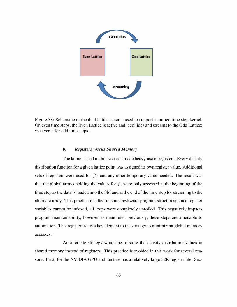
Figure 38: Schematic of the dual lattice scheme used to support a unified time step kernel.On even time steps, the Even Lattice is active and it collides and streams to the Odd Lattice;vice versa for odd time steps.

b. Registers versus Shared Memory

The kernels used in this research made heavy use of registers. Every density

distribution function for a given lattice point was assigned its own register value. Additional

sets of registers were used for f eqα and any other temporary value needed. The result was

that the global arrays holding the values for fα were only accessed at the beginning of the

time step as the data is loaded into the SM and at the end of the time step for streaming to the

alternate array. This practice resulted in some awkward program structures; since register

variables cannot be indexed, all loops were completely unrolled. This negatively impacts

program maintainability, however as mentioned previously, these steps are amenable to

automation. This register use is a key element to the strategy to minimizing global memory

accesses.

An alternate strategy would be to store the density distribution values in

shared memory instead of registers. This practice is avoided in this work for several rea-

sons. First, for the NVIDIA GPU architecture has a relatively large 32K register file. Sec-

63

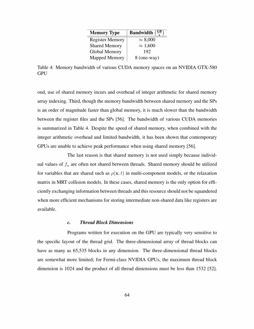
Memory Type Bandwidth(GB

s

)Register Memory ≈ 8,000Shared Memory ≈ 1,600Global Memory 192Mapped Memory 8 (one-way)

Table 4: Memory bandwidth of various CUDA memory spaces on an NVIDIA GTX-580GPU

ond, use of shared memory incurs and overhead of integer arithmetic for shared memory

array indexing. Third, though the memory bandwidth between shared memory and the SPs

is an order of magnitude faster than global memory, it is much slower than the bandwidth

between the register files and the SPs [56]. The bandwidth of various CUDA memories

is summarized in Table 4. Despite the speed of shared memory, when combined with the

integer arithmetic overhead and limited bandwidth, it has been shown that contemporary

GPUs are unable to achieve peak performance when using shared memory [56].

The last reason is that shared memory is not used simply because individ-

ual values of fα are often not shared between threads. Shared memory should be utilized

for variables that are shared such as ρ(x, t) in multi-component models, or the relaxation

matrix in MRT collision models. In these cases, shared memory is the only option for effi-

ciently exchanging information between threads and this resource should not be squandered

when more efficient mechanisms for storing intermediate non-shared data like registers are

available.

c. Thread Block Dimensions

Programs written for execution on the GPU are typically very sensitive to

the specific layout of the thread grid. The three-dimensional array of thread blocks can

have as many as 65,535 blocks in any dimension. The three-dimensional thread blocks

are somewhat more limited; for Fermi-class NVIDIA GPUs, the maximum thread block

dimension is 1024 and the product of all thread dimensions must be less than 1532 [52].

64

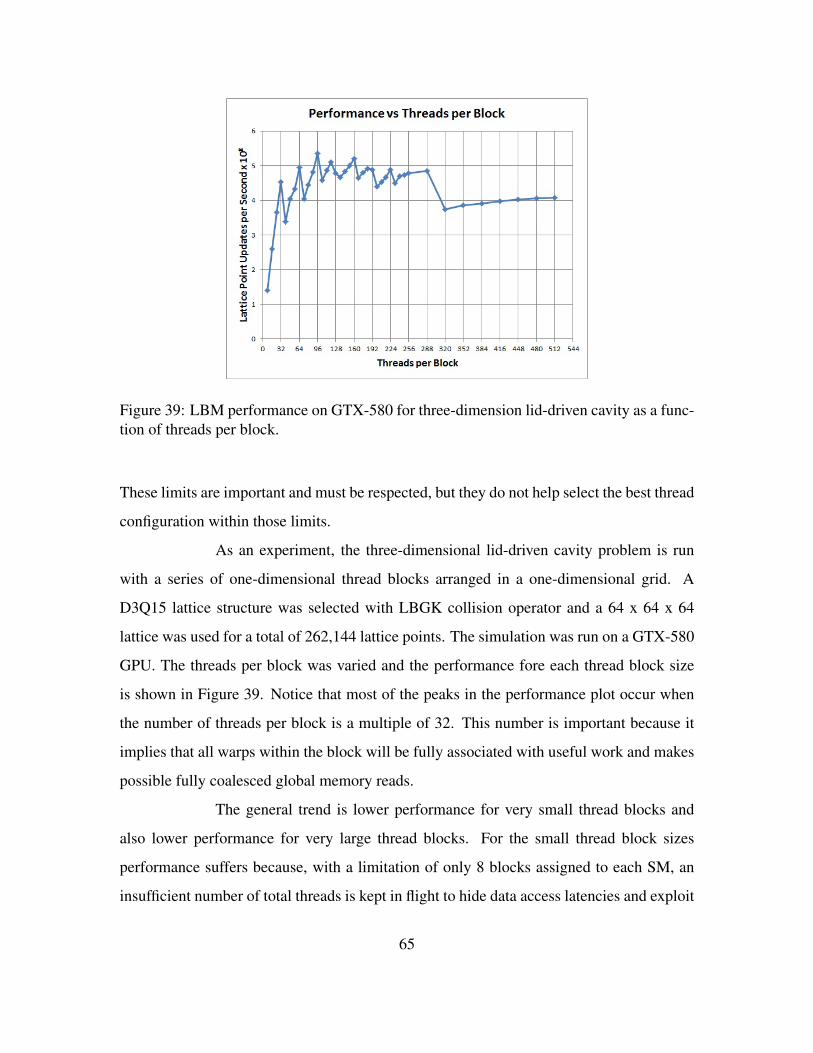
Figure 39: LBM performance on GTX-580 for three-dimension lid-driven cavity as a func-tion of threads per block.

These limits are important and must be respected, but they do not help select the best thread

configuration within those limits.

As an experiment, the three-dimensional lid-driven cavity problem is run

with a series of one-dimensional thread blocks arranged in a one-dimensional grid. A

D3Q15 lattice structure was selected with LBGK collision operator and a 64 x 64 x 64

lattice was used for a total of 262,144 lattice points. The simulation was run on a GTX-580

GPU. The threads per block was varied and the performance fore each thread block size

is shown in Figure 39. Notice that most of the peaks in the performance plot occur when

the number of threads per block is a multiple of 32. This number is important because it

implies that all warps within the block will be fully associated with useful work and makes

possible fully coalesced global memory reads.

The general trend is lower performance for very small thread blocks and

also lower performance for very large thread blocks. For the small thread block sizes

performance suffers because, with a limitation of only 8 blocks assigned to each SM, an

insufficient number of total threads is kept in flight to hide data access latencies and exploit

65

the full parallelism of the GPU. With very large thread blocks the reduced performance is

a combination of a reduced number of blocks per SM due to register resource limitations

resulting in an overall reduction in the number of threads in flight and accompanying loss

of parallel performance. With an intermediate number of threads which is also a multiple

of 32, more blocks are assigned to each SM, more total threads are kept in flight, SMs have

adequate resources to service the threads that are assigned to them.2

Though this was just one example case, the general trends are the same for

other LBM solvers developed for this work. As a summary for thread block selection, the

following summary is offered for use as a guideline.

• Choose thread block size that is a multiple of 32. This will en-

sure all thread warps are associated with useful work and allow for

efficient memory access.

• Choose a thread block size that is large enough to ensure enough

threads are in flight to hide memory access latencies.

• Choose a thread block size is not too large so that an individual SM

has adequate resources to execute at least one block at a time.

• For most problems, a good starting point is 128 threads per block.

These guidelines may be effective as a starting point for testing, but not as a rule that may

be used blindly. Ultimately, there does not appear to be an alternative to experimentation

to find the thread block size that is best for a given implementation of a given problem.

D. PERFORMANCE BENCHMARK–3D LID-DRIVEN CAVITY

In order to compare the effectiveness of the implementation strategies adopted for

this work, a three-dimensional lid-driven cavity problem was selected as a benchmark.2The main concern with too many threads is register spillage. If there are more register variables declared

in a kernel than can be accommodated by the register file, these excess variables are “spilled” to local memory.Local memory is private memory to each thread block but physically it is located on device global memory.Despite the use of level 1 and level 2 caching on new generation GPUs, performance is degraded when thishappens.

66

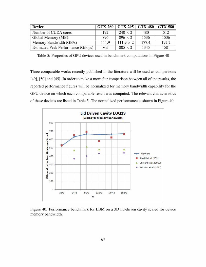
Device GTX-260 GTX-295 GTX-480 GTX-580Number of CUDA cores 192 240 × 2 480 512Global Memory (MB) 896 896 × 2 1536 1536Memory Bandwidth (GB/s) 111.9 111.9 × 2 177.4 192.2Estimated Peak Performance (Gflops) 805 805 × 2 1345 1581

Table 5: Properties of GPU devices used in benchmark computations in Figure 40

Three comparable works recently published in the literature will be used as comparisons

[49], [50] and [45]. In order to make a more fair comparison between all of the results, the

reported performance figures will be normalized for memory bandwidth capability for the

GPU device on which each comparable result was computed. The relevant characteristics

of these devices are listed in Table 5. The normalized performance is shown in Figure 40.

Figure 40: Performance benchmark for LBM on a 3D lid-driven cavity scaled for devicememory bandwidth.

67

It can be seen from Figure 40 that the result of this work is comparable to or bet-

ter than other recently reported implementations. It is somewhat surprising that the results

reported by Astorino et al. in [50] are so poor. In their paper, emphasis is made on the mod-

ularity and generality of the C++ implementation. While most implementations, including

this work, combine all elements of a LBM time step within a single kernel, the work de-

scribed in [50] is modular in the sense that computations concerning boundary conditions,

collision and streaming are separated into separate kernels that can be individually main-

tained. While it is conceded in this work that software engineering considerations such as

maintainability and ease of future expansion are laudable, those considerations often take a

back seat to performance due to the higher demands on memory bandwidth due to the need

to store intermediate variables.

In order to achieve the best performance for each problem size, the number of

threads per block must be adjusted accordingly. The dependence of execution performance

on the thread block size is illustrated in Figure 41. Using 96 threads per block performs

well for all problem sizes, while the use of 256 threads in a block performs very poorly for

all problem sizes.

E. HYBRID PARALLEL LBM

Though excellent execution performance on LBM problems can be achieved when

the program is executed on a GPU, it is inevitable that the need will arise to perform sim-

ulations for which the basic data variables are too numerous to store in the global memory

of a single GPU. The programs ultimately have to scale to multiple devices. For this work,

the GPU-based implementation with CUDA on an NVIDIA GPU is coupled with tradi-

tional parallel programming methodologies. First, the GPU-accelerated LBM code will be

augmented with OpenMP directives to allow execution on multiple GPUs installed on a

single workstation. Second, the GPU-accelerated code will instead be employed within a

distributed programming environment using MPI.

68

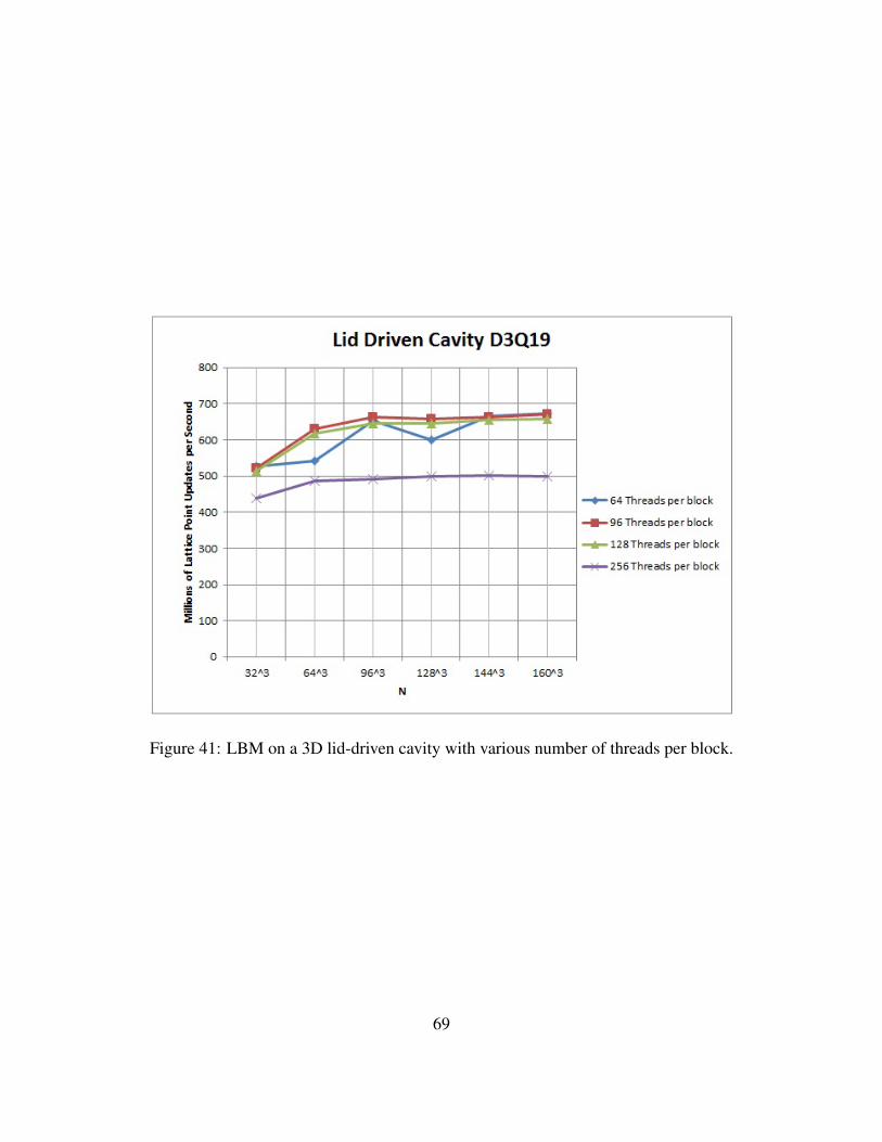
Figure 41: LBM on a 3D lid-driven cavity with various number of threads per block.

69

1. CUDA with OpenMP

When multiple GPUs are used, it may be taken to imply that a distributed memory

programming model must be employed. Since none of the devices are capable of han-

dling the entire domain, it is logical that the domain must be partitioned with relevant data

distributed among the devices.3 However, for workstations equipped with multiple GPUs,

the use of CUDA alongside of OpenMP is an attractive option. Since all of the devices

are physically located on the same machine, it is convenient to use the shared-memory

paradigms of OpenMP rather than explicitly dealing with the message passing API of MPI.

For this work, a workstation equipped with six NVIDIA C2070 GPUs is employed

to execute the three-dimensional lid-driven cavity problem with both CUDA and OpenMP.

The problem domain is partitioned geometrically among the available devices and inter-

partition boundary data is exchanged between the devices in a peer-to-peer mode. Though

the bandwidth capability of the PCIe bus is still a limitation, the demand is comparatively

low since only boundary data is exchanged.

Performance results for the three-dimensional lid driven cavity problem is shown in

Figure 42. For the simulation a D3Q15 lattice was used with LBGK collision operator. The

lattice size was set to 500x500x500 lattice for a total of 125 million lattice points. It can be

seen that the scaling is somewhat less than linear. This is attributed primarily to the fact that

this particular multi-GPU implementation that does not overlap computations with peer-to-

peer communications. Future CUDA/OpenMP will incorporate this optimization and is

expected to improve scalability.

2. CUDA with MPI

Though using CUDA in conjunction with OpenMP makes it possible to employ

multiple GPUs to bring larger problem sizes into reach, this solution still has limitations in

3Strictly speaking, this is not true. With recent GPUs operating computers with sufficient physical mem-ory and a 64-bit operating system, it is possible to maintain the entire problem in the (usually larger) CPUsystem memory with each sub domain logically mapped to the GPU that will be assigned to carry out itscomputations. Unfortunately, the memory transfer overhead across the comparatively slow 8 GB/sec PCIebus from the CPU memory to the GPU renders this convenient programming technique impractical.

70

Figure 42: Lid-driven cavity using a D3Q15 lattice with 5003 points using CUDA andOpenMP.

scalability. While it is conceivable that workstations will be constructed capable of hosting

more than six GPUs and that each GPU will gradually increase its memory size thus be

capable of handling larger problems, the need currently exists to model fluid problems

using LBM that require billions of lattice points and must be simulated for millions of time

steps. In order to scale to these problem sizes, it is necessary to develop LBM codes that

can be deployed cooperatively on an arbitrarily large number of nodes.

The standard programming paradigm for programs of this type is to use a distributed

parallel programming model based on MPI. When developing a program that uses MPI it

is critically important that the algorithm is implemented such that necessary computations

are interleaved with any communication requirements that may exist for the problem. In

addition to high-performance CPUs, the other key feature that the hardware on which the

code is to run must posses is high-speed interconnects. For this work, a test code that

used only MPI with CPUs was developed to analyze three-dimensional Poiseuille flow.

The lattice points throughout the domain were partitioned geometrically and distributed as

evenly as possible to all available processors.

71

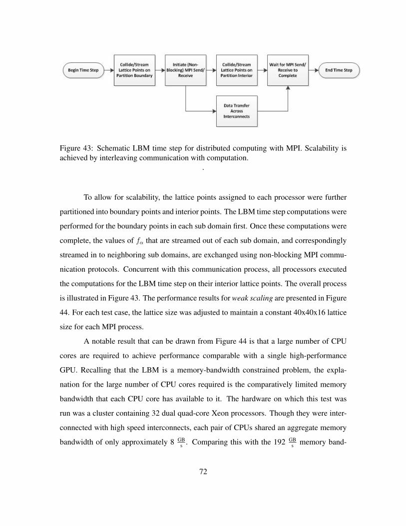
Figure 43: Schematic LBM time step for distributed computing with MPI. Scalability isachieved by interleaving communication with computation.

.

To allow for scalability, the lattice points assigned to each processor were further

partitioned into boundary points and interior points. The LBM time step computations were

performed for the boundary points in each sub domain first. Once these computations were

complete, the values of fα that are streamed out of each sub domain, and correspondingly

streamed in to neighboring sub domains, are exchanged using non-blocking MPI commu-

nication protocols. Concurrent with this communication process, all processors executed

the computations for the LBM time step on their interior lattice points. The overall process

is illustrated in Figure 43. The performance results for weak scaling are presented in Figure

44. For each test case, the lattice size was adjusted to maintain a constant 40x40x16 lattice

size for each MPI process.

A notable result that can be drawn from Figure 44 is that a large number of CPU

cores are required to achieve performance comparable with a single high-performance

GPU. Recalling that the LBM is a memory-bandwidth constrained problem, the expla-

nation for the large number of CPU cores required is the comparatively limited memory

bandwidth that each CPU core has available to it. The hardware on which this test was

run was a cluster containing 32 dual quad-core Xeon processors. Though they were inter-

connected with high speed interconnects, each pair of CPUs shared an aggregate memory

bandwidth of only approximately 8 GBs . Comparing this with the 192 GB

s memory band-

72

Figure 44: Weak scaling using MPI for LBM simulation of three-dimensional Poiseuilleflow.

width of an NVIDIA GTX-580 GPU, having a memory bandwidth advantage of 24 to 1. In

this light, it is not surprising that nearly 200 CPU cores were required. It is conceded that

higher performance computer systems would have yielded better CPU results.

The key insight that this work seeks to demonstrate is that the GPU brings concen-

trated scalable performance. A collection of GPUs which individually have high memory

bandwidth, coupled with high-speed interconnects, can effectively combine their aggre-

gate memory bandwidth and compute capability using fewer devices than is necessary with

CPUs. This will only remain true so long as GPUs maintain their overwhelming superior-

ity in memory bandwidth. When that advantage is lost, the GPUs will also have lost their

advantage for high performance scientific computing.

To demonstrate the scalability of a hybrid parallel LBM implementation with CUDA

and MPI, the same three-dimensional Poiseuille flow was tested on a system with two nodes

and two GPUs per node. The results are presented in Figure 45. In this instance, the results

are not as encouraging as that obtained using CUDA and OpenMP. This is attributed at

least in part to the fact that the CUDA/OpenMP case was able to take advantage of highly

73

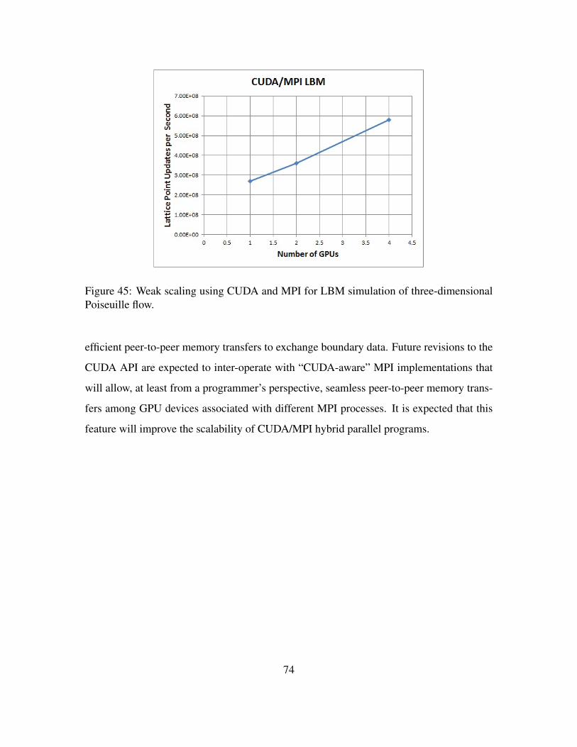
Figure 45: Weak scaling using CUDA and MPI for LBM simulation of three-dimensionalPoiseuille flow.

efficient peer-to-peer memory transfers to exchange boundary data. Future revisions to the

CUDA API are expected to inter-operate with “CUDA-aware” MPI implementations that

will allow, at least from a programmer’s perspective, seamless peer-to-peer memory trans-

fers among GPU devices associated with different MPI processes. It is expected that this

feature will improve the scalability of CUDA/MPI hybrid parallel programs.

74

V. FLUID-STRUCTURE INTERACTION WITH LBM

The principle goal of this research is to investigate the use of LBM for FSI. With

a working collection of LBM tools to model a variety of flow conditions in both two and

three dimensions it is necessary to couple these tools with the requisite structural models to

analyze FSI. Following a brief literature review, the coupled FSI problem will be explored

in turn for the 2D and 3D case. The chief products of these investigations are:

• A collection of example problems to be compared with previous work and

established benchmarks. Each example problem illustrates qualitatively

the coupled interaction between the fluid flow and a linear elastic structure

with small displacements.

• A novel algorithm for exploiting task-level parallelism inherent in the FSI

problem that exploits both the CPU as well as the GPU to make best use

of computational resources and achieve high performance.

Despite these advances, significant work remains to be done in this area in order to

allow reliable and effective FSI over a range of interesting problem domains. In particular,

geometric and material nonlinearity must be incorporated into the material model in order

to quantitatively match benchmark data. Additionally, in order to accommodate the large

structural displacements, the LBM model must be further expanded to account for lattice

points transitioning from the fluid domain to that subdomain covered by the solid when the

structure undergoes large displacements.

A. INTRODUCTION AND LITERATURE REVIEW

The interaction of fluid flow with elastic structures and suspended particles are com-

monly encountered problems in many practical engineering applications. Use of the LBM

for the fluid modeling is common, nonetheless to the best the author’s knowledge no sub-

stantial work has been done to apply LBM to solve the equations of structural dynamics.

75

Consequently, several methods have been proposed to couple the LBM with more tradi-

tional structural dynamics solvers in order to collectively capture both the fluid and struc-

tural dynamics aspects FSI problems.

Some recent authors, such as [59], [60] and [61], have used the immersed boundary

(IB) method along with LBM. In an IB method, the fluid problem is solved over a fixed

Eulerian grid that covers the entire domain. The immersed boundary is solved on a moving

Lagrangian array of points overlying a portion of the Eulerian grid. The force that the fluid

exerts on the moving boundary is projected onto the Lagrangian node points by use of the

Dirac delta function as described in [62]. This solution procedure has been extensively

used for studying FSI applications, particularly for biological flows [63].

While the IB method has been popular for modeling of highly flexible structures,

a common methodology for multibody coupling with the LBM is the discrete element

method (DEM). This method combines problems addressed by the coupled IB and LBM

solvers, and indeed, use the same methods for hydrodynamic coupling between the fluid

and solid, but also account for the solid body-to-body interactions and has been extensively

used for particle and granular flow problems. A succinct review of the use of LBM and

DEM is provided in [64]. As a few examples, this approach has found use in investigation

of sedimentation of particles in fluid at low Reynolds numbers [65], particulate flows [66],

and particle transport in turbulent fluid flows [67].

The FEM has a long history of use for problems in both structural and fluid dynam-

ics. As can be expected, the FEM as also been applied to FSI problems where the FEM

is used in both the fluid and solid domains [68], [69] and [70], for example. In this work,

the advances in coupling LBM with FEM for structural dynamics presented in [28] will be

used as a starting point for further FSI studies.

B. FORCE EVALUATION

All aforementioned approaches to coupled FSI problems share the issue of needing

to determine how forces and momentum inputs from one domain are to be transmitted into

76

the other. For monolithic approaches, such as using FEM both for the fluid and structural

domains, the transfer of this data may be a natural part of the discretization and satisfaction

of continuity equations. For the coupled LBM and FEM approach undertaken in this work,

it is necessary to obtain the force that the fluid imparts upon this structure at the fluid-solid

interface. Two approaches will be discussed in this section:

1. Stress Integration Approach; and

2. Momentum Response Approach

1. Stress Integration Approach

This method was introduced by He and Doolen in [71], where they evaluated the

forces on a cylinder in channel flow by integrating the total stresses on the surface of the

cylinder by evaluating Equation 45,

F =

∫n ·[pI + ρν

(∇u + (∇u)T

)]dA (45)

where F is the force vector, n is the outward facing normal of a the solid surface, and ν is

the kinematic viscosity.

The first term of Equation 45 is easy to evaluate within the LBM framework using

the simple relation of Equation 13 from Chapter II. The second term in Equation 45 is the

deviatoric stress for incompressible flow as given in Equation 46.

τij = ρν(∇u + (∇u)T

)(46)

Equation 46 can be evaluated by computing the macroscopic velocity throughout the do-

main using Equation 12, then a using a discrete differencing scheme to compute the spatial

partial derivatives and evaluate τij with given values of viscosity. This methodology does

not sit well with the general theme of LBM whereby computations should be performed

locally to a single lattice point. In keeping with the general theme of locality, in LBM τij is

77

computed using the non-equilibrium portion of the particle density distribution function;

f neqα = fα − f eq

α . In the case for a D2Q9 lattice, at each lattice point this is done using

Equation 47

τij =

(1− 1

2τ

) 8∑α=1

[fα (x, t)− f (eq)

α (x, t)]×(

eαieαj −1

2eα · eαδij

)(47)

Once the integrand for Equation 45 is computed, executing the integral can be done numer-

ically with, for the D2Q9 lattice with Equation 48.

F =4∑

α=1

eα ·[pI + ρν

(∇u + (∇u)T

)]δx (48)

In summary, to use the stress integration approach for evaluating fluid forces on a

structure, given fluid viscosity and the current set of density distribution functions fα:

1. Compute density using Equation 11.

2. With this density, compute pressure using Equation 13.

3. Compute macroscopic velocity using Equation 12.

4. Compute f eqα using Equation 10.

5. Compute local deviatoric stress via Equation 47.

6. Compute force from surface stress with Equation 48.

2. Momentum Response Approach

Instead of the stress integration method, a momentum exchange method, developed

by Ladd in [72], can be used to compute the fluid force on closed surfaces suspended in the

flow field. In this method, the total force acting on a solid body is obtained by Equation 49,

78

F =∑allxb

Nd∑α=1

eα [fα(xb, t) + fα (xb + eαδt, t)] (49)

where eα is the lattice direction opposite of eα.

One disadvantage of the momentum response as shown in Equation 49 is that it

makes use of values of fα from neighboring lattice points. This non-locality can compli-

cate parallel implementation. For problems with a large number of lattice points on fluid/-

solid boundaries, the need to access additional values of fα can add to the overall memory

bandwidth demand and thus degrade performance for this memory bandwidth-bound ap-

plication.

C. COUPLING PROCEDURE

Once the relevant forces have been computed on the fluid domain, they must be

satisfactorily transferred to the discrete representation of the structural domain on which

they will be imparted. Respectively, once the equations of motion have been solved on

the structural domain, the inputs relevant to the coupled fluid problem must be passed

to the fluid domain. This straight-forward problem can become complicated due to the

possibility that the discrete representation of the fluid and solid may not conform exactly

at the interface. In cases where the meshes do not conform, some form of interpolation

will be required in order to map forces applied in one domain to degrees of freedom in the

other.

For this work, problems were restricted to those where the fluid and structural dis-

cretizations would conform at domain boundaries. This approach greatly simplifies com-

munication of information between domains at the cost of severely restricting the types of

problems that can be analyzed. Specifically, the geometric non-linearity of a moving solid

mesh covering and uncovering fluid lattice points is not addressed within the scope of the

79

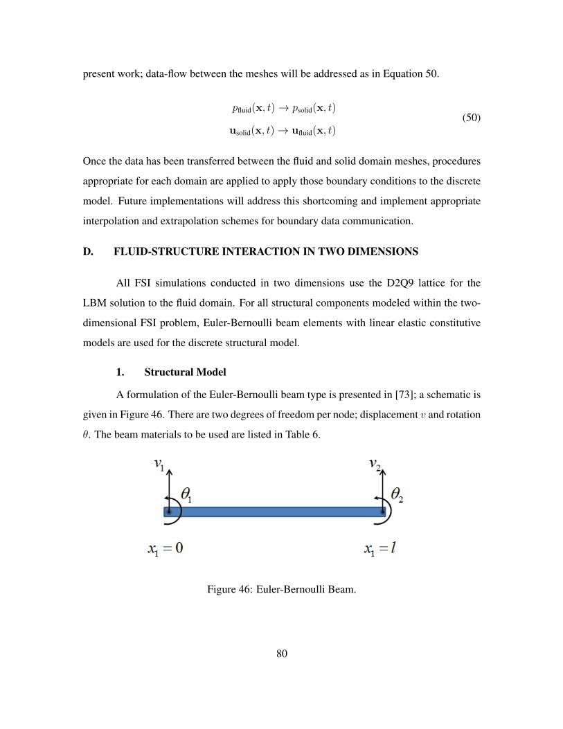
present work; data-flow between the meshes will be addressed as in Equation 50.

pfluid(x, t)→ psolid(x, t)

usolid(x, t)→ ufluid(x, t)(50)

Once the data has been transferred between the fluid and solid domain meshes, procedures

appropriate for each domain are applied to apply those boundary conditions to the discrete

model. Future implementations will address this shortcoming and implement appropriate

interpolation and extrapolation schemes for boundary data communication.

D. FLUID-STRUCTURE INTERACTION IN TWO DIMENSIONS

All FSI simulations conducted in two dimensions use the D2Q9 lattice for the

LBM solution to the fluid domain. For all structural components modeled within the two-

dimensional FSI problem, Euler-Bernoulli beam elements with linear elastic constitutive

models are used for the discrete structural model.

1. Structural Model

A formulation of the Euler-Bernoulli beam type is presented in [73]; a schematic is

given in Figure 46. There are two degrees of freedom per node; displacement v and rotation

θ. The beam materials to be used are listed in Table 6.

Figure 46: Euler-Bernoulli Beam.

80

Material ρ( kg

m3

)E( kg

m2

)× 106

steel 7,800 210,000cork 180 32PVC 1,400 1,500

Table 6: Selected structural material properties used for FSI simulations.

Fluid ρ( kg

m3

)ν(

m2

sec

)× 10−6

ethyl alcohol 790 1.4vegetable oil 920 76.1water 1000 1.14blood 1035 4glycerin 1260 1127Mercury 13594 0.0114

Table 7: Selected fluid properties for FSI simulations.

2. Fluid Models

The FSI simulations performed for this work were repeated for a selected combina-

tion of fluid and structural properties. The goal is to obtain insight as to how the combined

systems would behave with various combinations of either highly viscous and dense fluids

like honey as compared to fluids of very low viscosity such as liquid Mercury. Though this

leads to an admittedly qualitative analysis, this author asserts that the results can still be

useful for building intuition and confirming the overall efficacy of the software tools. The

relevant properties of the fluids used in these simulations are summarized in Table 7.

3. Converging-Diverging Channel

This problem, inspired by similar work reported in [74], is a 2D FSI problem of

flow in a converging and diverging duct. A schematic of the problem domain is shown in

Figure 47. No-slip boundary conditions are used on the rigid portions of the upper and

lower boundary. In the LBM problem, the structure is modeled as a moving solid domain

and in the FEM structural dynamics problem it is modeled as a Euler-Bernoulli beam with

clamped boundary conditions on both ends.

81

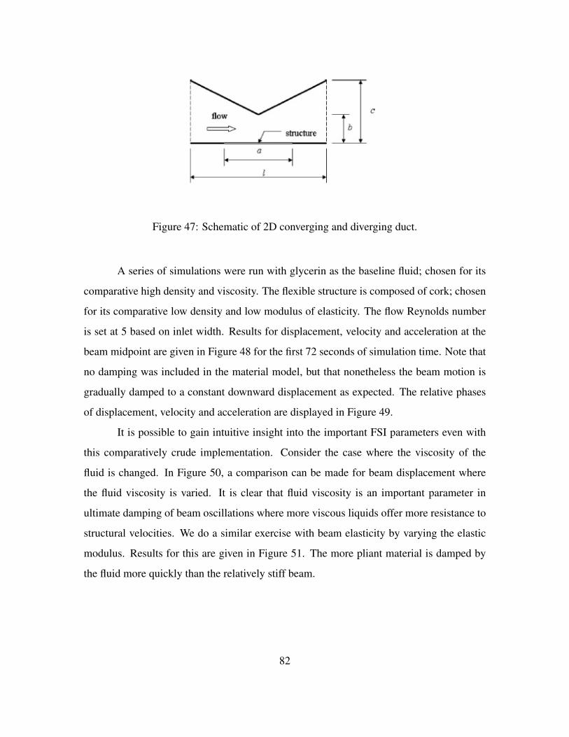
Figure 47: Schematic of 2D converging and diverging duct.

A series of simulations were run with glycerin as the baseline fluid; chosen for its

comparative high density and viscosity. The flexible structure is composed of cork; chosen

for its comparative low density and low modulus of elasticity. The flow Reynolds number

is set at 5 based on inlet width. Results for displacement, velocity and acceleration at the

beam midpoint are given in Figure 48 for the first 72 seconds of simulation time. Note that

no damping was included in the material model, but that nonetheless the beam motion is

gradually damped to a constant downward displacement as expected. The relative phases

of displacement, velocity and acceleration are displayed in Figure 49.

It is possible to gain intuitive insight into the important FSI parameters even with

this comparatively crude implementation. Consider the case where the viscosity of the

fluid is changed. In Figure 50, a comparison can be made for beam displacement where

the fluid viscosity is varied. It is clear that fluid viscosity is an important parameter in

ultimate damping of beam oscillations where more viscous liquids offer more resistance to

structural velocities. We do a similar exercise with beam elasticity by varying the elastic

modulus. Results for this are given in Figure 51. The more pliant material is damped by

the fluid more quickly than the relatively stiff beam.

82

Figure 48: Converging and diverging duct displacement, velocity and acceleration at beammidpoint. Re = 5, glycerin with cork beam.

83

_,

10 20 30 40 Time (sec)

Time (sec)

Time (sec)

50 60 70 80

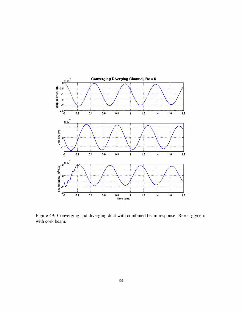
Figure 49: Converging and diverging duct with combined beam response. Re=5, glycerinwith cork beam.

84

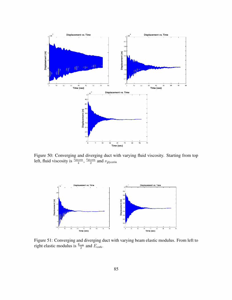
Figure 50: Converging and diverging duct with varying fluid viscosity. Starting from topleft, fluid viscosity is νglycerin

4, νglycerin

2and νglycerin

Figure 51: Converging and diverging duct with varying beam elastic modulus. From left toright elastic modulus is Ecork

2and Ecork.

85

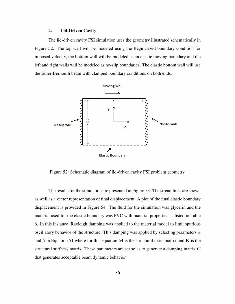
4. Lid-Driven Cavity

The lid-driven cavity FSI simulation uses the geometry illustrated schematically in

Figure 52. The top wall will be modeled using the Regularized boundary condition for

imposed velocity, the bottom wall will be modeled as an elastic moving boundary and the

left and right walls will be modeled as no-slip boundaries. The elastic bottom wall will use

the Euler-Bernoulli beam with clamped boundary conditions on both ends.

Figure 52: Schematic diagram of lid-driven cavity FSI problem geometry.

The results for the simulation are presented in Figure 53. The streamlines are shown

as well as a vector representation of final displacement. A plot of the final elastic boundary

displacement is provided in Figure 54. The fluid for the simulation was glycerin and the

material used for the elastic boundary was PVC with material properties as listed in Table

6. In this instance, Rayleigh damping was applied to the material model to limit spurious

oscillatory behavior of the structure. This damping was applied by selecting parameters α

and β in Equation 51 where for this equation M is the structural mass matrix and K is the

structural stiffness matrix. These parameters are set so as to generate a damping matrix C

that generates acceptable beam dynamic behavior.

86

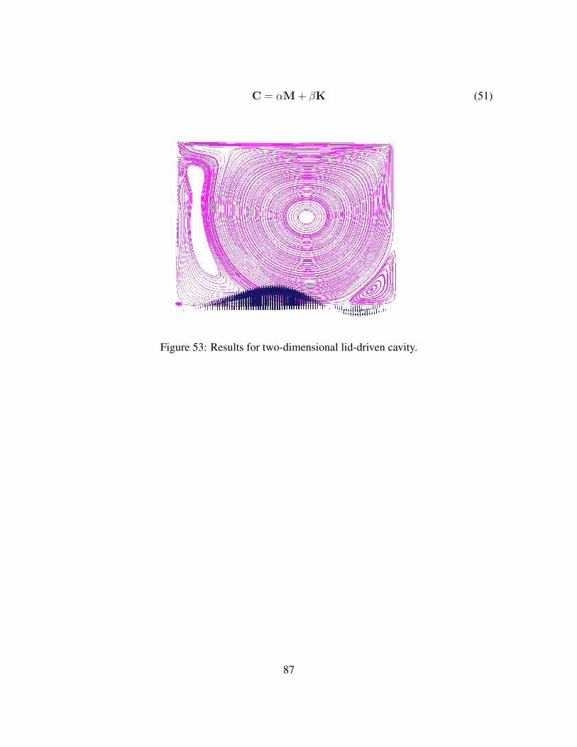
C = αM + βK (51)

Figure 53: Results for two-dimensional lid-driven cavity.

87

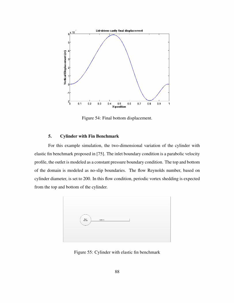
Figure 54: Final bottom displacement.

5. Cylinder with Fin Benchmark

For this example simulation, the two-dimensional variation of the cylinder with

elastic fin benchmark proposed in [75]. The inlet boundary condition is a parabolic velocity

profile, the outlet is modeled as a constant pressure boundary condition. The top and bottom

of the domain is modeled as no-slip boundaries. The flow Reynolds number, based on

cylinder diameter, is set to 200. In this flow condition, periodic vortex shedding is expected

from the top and bottom of the cylinder.

Figure 55: Cylinder with elastic fin benchmark

88

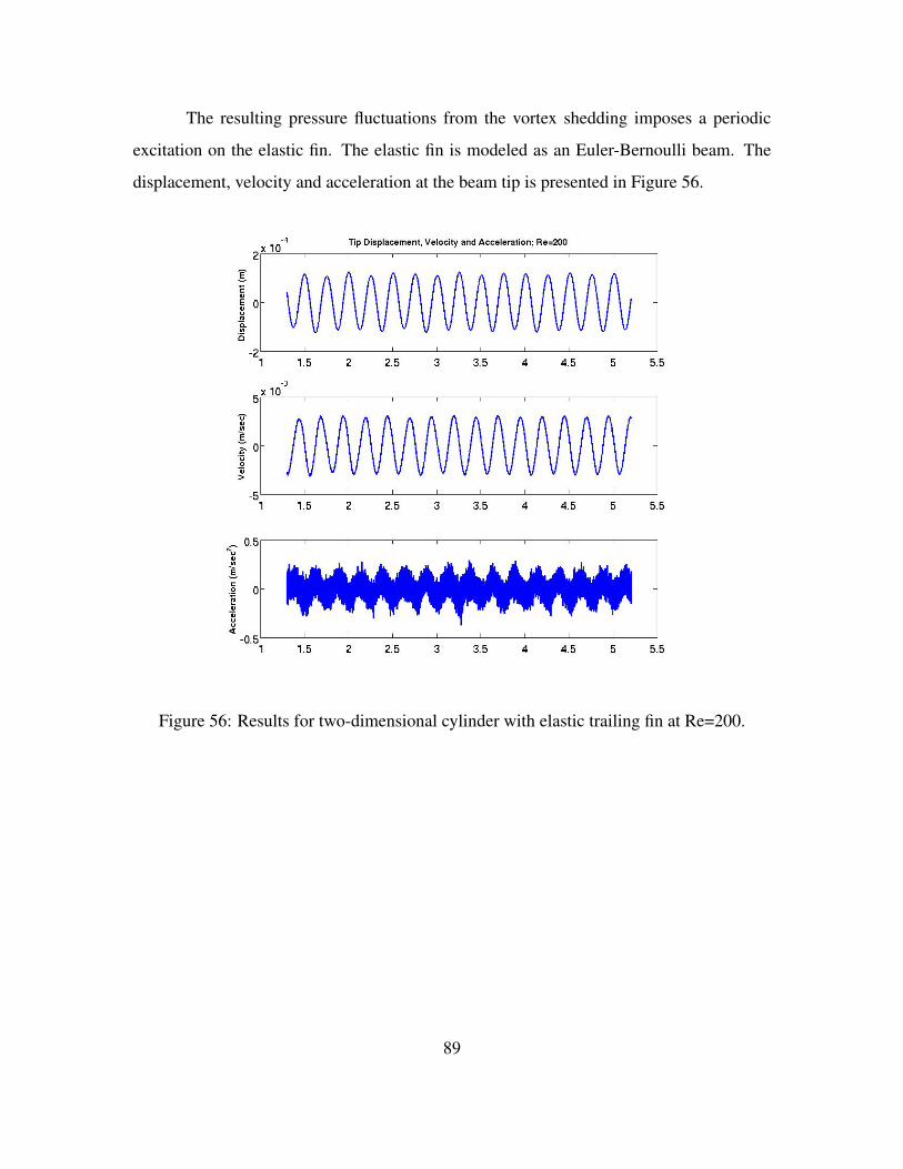
The resulting pressure fluctuations from the vortex shedding imposes a periodic

excitation on the elastic fin. The elastic fin is modeled as an Euler-Bernoulli beam. The

displacement, velocity and acceleration at the beam tip is presented in Figure 56.

Figure 56: Results for two-dimensional cylinder with elastic trailing fin at Re=200.

89

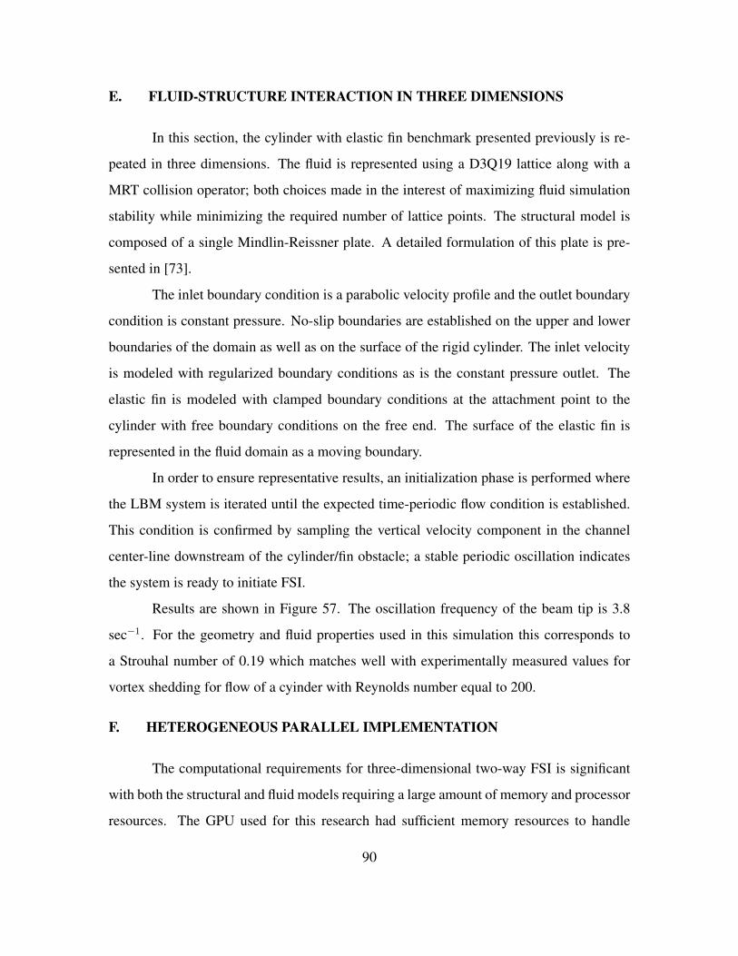
E. FLUID-STRUCTURE INTERACTION IN THREE DIMENSIONS

In this section, the cylinder with elastic fin benchmark presented previously is re-

peated in three dimensions. The fluid is represented using a D3Q19 lattice along with a

MRT collision operator; both choices made in the interest of maximizing fluid simulation

stability while minimizing the required number of lattice points. The structural model is

composed of a single Mindlin-Reissner plate. A detailed formulation of this plate is pre-

sented in [73].

The inlet boundary condition is a parabolic velocity profile and the outlet boundary

condition is constant pressure. No-slip boundaries are established on the upper and lower

boundaries of the domain as well as on the surface of the rigid cylinder. The inlet velocity

is modeled with regularized boundary conditions as is the constant pressure outlet. The

elastic fin is modeled with clamped boundary conditions at the attachment point to the

cylinder with free boundary conditions on the free end. The surface of the elastic fin is

represented in the fluid domain as a moving boundary.

In order to ensure representative results, an initialization phase is performed where

the LBM system is iterated until the expected time-periodic flow condition is established.

This condition is confirmed by sampling the vertical velocity component in the channel

center-line downstream of the cylinder/fin obstacle; a stable periodic oscillation indicates

the system is ready to initiate FSI.

Results are shown in Figure 57. The oscillation frequency of the beam tip is 3.8

sec−1. For the geometry and fluid properties used in this simulation this corresponds to

a Strouhal number of 0.19 which matches well with experimentally measured values for

vortex shedding for flow of a cyinder with Reynolds number equal to 200.

F. HETEROGENEOUS PARALLEL IMPLEMENTATION

The computational requirements for three-dimensional two-way FSI is significant

with both the structural and fluid models requiring a large amount of memory and processor

resources. The GPU used for this research had sufficient memory resources to handle

90

Figure 57: Displacement, velocity and acceleration for cylinder with elastic fin. Re=200.

91

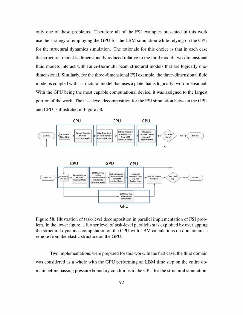
only one of these problems. Therefore all of the FSI examples presented in this work

use the strategy of employing the GPU for the LBM simulation while relying on the CPU

for the structural dynamics simulation. The rationale for this choice is that in each case

the structural model is dimensionally reduced relative to the fluid model; two-dimensional

fluid models interact with Euler-Bernoulli beam structural models that are logically one-

dimensional. Similarly, for the three-dimensional FSI example, the three-dimensional fluid

model is coupled with a structural model that uses a plate that is logically two-dimensional.

With the GPU being the most capable computational device, it was assigned to the largest

portion of the work. The task-level decomposition for the FSI simulation between the GPU

and CPU is illustrated in Figure 58.

Figure 58: Illustration of task-level decomposition in parallel implementation of FSI prob-lem. In the lower figure, a further level of task-level parallelism is exploited by overlappingthe structural dynamics computation on the CPU with LBM calculations on domain areasremote from the elastic structure on the GPU.

Two implementations were prepared for this work. In the first case, the fluid domain

was considered as a whole with the GPU performing an LBM time step on the entire do-

main before passing pressure boundary conditions to the CPU for the structural simulation.

92

When the CPU completed the structural time-step, velocity boundary conditions are passed

back to the GPU. In the second case, the fluid domain is partitioned as illustrated in Figure

59. With this decomposed domain, the GPU would execute an LBM time step in a region

of the domain immediately surrounding the elastic structure. When the time step is com-

plete, updated fluid forces are transferred to the CPU memory so that the structural time

step can be executed. Concurrently, immediately upon passing its boundary conditions, the

GPU commences execution of the LBM time step on the remaining fluid domain. In this

way, the overall computation time is reduced by exploiting this extra level of concurrency.

The performance improvement that is realized by using this strategy is highly variable; de-

pending both on the problem as well as the relative performance characteristics of the GPU

and CPU as well as the implementation details of both the LBM and structural dynamics

simulation model. Nonetheless, for this research, using an Intel i5 quad-core CPU running

at 3.6 GHz combined with a NVIDA GTX-580, a performance improvement of 23% was

obtained using this procedure as shown in Table 8.

Figure 59: Decomposition of FSI problem domain for task-level heterogeneous parallelism.

93

Method Average time per time-step (sec) Percent SpeedupNon-Overlapped 0.0305 -Overlapped 0.0234 23%

Table 8: Performance improvement from using overlapped execution depicted in lowerhalf of Figure 58 versus the non-overlapped scheme in the top half of Figure 58. The latticewas 22 x 337 x 526 D3Q19 using MRT collision operator. The structural model was asheer-deformable plate with 2883 degrees of freedom.

94

VI. HYBRID LATTICE BOLTZMANN METHOD

A. INTRODUCTION AND LITERATURE REVIEW

As a fluid flow solver, the LBM is particularly effective in scenarios where con-

ventional methods like FDM, CVM and FEM have difficulty. Cases with highly complex

geometry such as are encountered in porous flow problems [76] where it is difficult or

impractical to fully discretize the domain are particularly suitable to LBM. Simulations

involving multi-component or multi-phase flows where it is very hard to accurately model

fluid interfaces and to capture fluid phase and component interactions are also examples

where LBM has found good use [77]-[79].

Despite these advantages, the LBM in its classical formulation (CLBM) has chal-

lenges of its own. In order to describe the transport of particle velocity distributions through

the domain, the CLBM calls for a coupled space and time domain discretization that is re-

alized in the form of a uniform and regular set of lattice points across which particles

“stream.” For practical problems which often contain objects with curved or complex sur-

faces it may be necessary to use a highly refined lattice to describe the geometry. This often

leads to non-complex regions of the domain populated with a needlessly dense lattice.

Several methods have been developed to alleviate this issue and provide greater

geometric flexibility and adaptability to the lattice mesh. These approaches include de-

velopment of a finite volume formulation of the LBM [80] as well as finite difference

formulations [81], [82], multigrid lattice methods [83] finite element LBM (FELBM) [84],

[74], and spectral element discontinuous Galerkin LBM [85]-[87] among others. These

methods obtain this benefit of geometric flexibility at the expense of a relative increase in

the computational effort required per lattice point in the problem domain.

In this dissertation, we describe a hybrid LBM (HLBM) where the FELBM derived

in [74] is combined with the CLBM over one or more sub-domains. This new method ex-

ploits the geometric flexibility of the FELBM to mesh complex surfaces with fewer lattice

95

points than the CLBM while leveraging the CLBM to model geometrically simple regions

of the problem domain with greater computational efficiency. The result is a method that

benefits from both approaches.

In the following section, the derivation of FELBM is outlined. Next, the coupling

procedure of the HLBM is illustrated followed by numerical results and conclusions.

B. FINITE ELEMENT LBM

The FELBM borrows almost everything from the CLBM theory. The formulation

and implementation can be summarized as very similar to CLBM with the exception of the

“streaming” procedure at the end of each time step which the FELBM does not do. Instead,

an equivalent operator is developed to “advect” the particle density distribution functions

along each of the characteristic lattice directions. This feature is what allows the FELBM

to use a non-uniform grid and the interpolative nature of the advection operator is common

among non-classical LBM procedures.

Starting with the discrete Boltzmann equation, we expand fα within a space of

interpolating polynomials defined on finite elements:

fα =n∑i=1

H if iα = [H]fα (52)

where n is the number of nodes in an element as well as the number of interpolating poly-

nomials H i.

This relation is substituted into Equation 8 using the BGK collision operator of

Equation 9 and the result is re-expressed in residual form:

R = [H]∂fα∂t

+ eα · [∇H]fα+1

τ[H]

(fα − fα

). (53)

Using the Galerkin formulation of the Method of Weighted Residuals, the given residual

is multiplied by the interpolating functions H i and integrated over all elemental domains.

This results in the following set of linear equations:

96

[M ]∂Fα∂t

+ [K]Fα+ [C]Fα − [C]Fα = 0 (54)

where, with Ωe being the elemental domain for the e-th finite element, the linear operators

are defined as:

[M ] =∑e

∫Ωe

[H]T [H]dΩ (55)

[K] =∑e

∫Ωe

[H]T (eα · [∇H]dΩ (56)

[C] =∑e

∫Ωe

1

τ[H]T [H]dΩ (57)

Fα =∑e

f eα. (58)

This is now a first-order differential equation in time which describes the advection of

particle distribution functions along the characteristic lattice directions.

Herein lies the difficulty of the FELBM. While the CLBM is able to accomplish the

particle “advection” by streaming between neighboring lattice points which can be effected

by simple copy and assignment operations, the FELBM must accomplish the same task

by evaluating this discrete linear advection equation. Whatever time integration method

is used, it is obvious that it will always be more demanding than the CLBM streaming

and, unlike the logical streaming method, is subject to the usual dissipative and dispersive

approximation errors associated with the numerical time-integration method employed.

Numerical dissipation and dispersion can be mitigated by reducing time-step size

and refining the spatial mesh, but both of those methods require more computational work.

In a similar way, dipsersive errors can be mitigated by using higher-level time integration

97

schemes such as explicit multi-stage Runge Kutta methods, or implicit methods such as

Backward Euler, Trapezoidal or Crank-Nicolson techniques but these methods also require

additional work.

The hybrid method introduced in the next section seeks to reduce the additional

computational workload associated by employing the FELBM over only those sub-domains

where the geometric flexibility is needed. The remainder of the domain is modeled with

CLBM and a coupling procedure is introduced to allow the solution to proceed concurrently

on all sub-domains.

C. HYBRID CLBM/FELBM METHODOLOGY

In order to mitigate the computational demands of the FELBM while retaining the

ability to model a domain with complex and irregular shapes without an unnecessarily

dense lattice, the hybrid CLBM/FELBM (HLBM) methodology is developed.

All of the theoretical machinery from the CLBM and FELBM formulations are

preserved and the logical sequence of computations is maintained on each individual sub-

domain. A typical HLBM time-step is portrayed schematically in Figure 60.

To couple disjoint sub-domains, an interface layer is provided. Computationally,

the streaming process of the CLBM domain and the advection process of the FELBM

domain can be executed concurrently with each sub-domain retaining a “halo” of depth

1 into the adjoining sub-domain. Within each sub-domain, the outermost layer of lattice

points represents the halo and as shown in Figure 61 and Figure 62.

While this coupling scheme is conceptually very simple, great care must be taken

with the time and space integration methods used for advecting particle density data on the

FELBM sub-domain. First-order time integration schemes tend to have too much dissipa-

tion error while second order schemes suffer from dispersion errors; both of which prop-

agate onto the CLBM sub-domain and impacts solution quality and stability everywhere.

For the results discussed in this paper, simple bi-linear elements are used for the spatial

discretization and a 4-stage 3rd order explicit time integration method shown in Equation

98

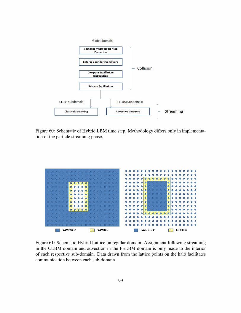
Figure 60: Schematic of Hybrid LBM time step. Methodology differs only in implementa-tion of the particle streaming phase.

Figure 61: Schematic Hybrid Lattice on regular domain. Assignment following streamingin the CLBM domain and advection in the FELBM domain is only made to the interiorof each respective sub-domain. Data drawn from the lattice points on the halo facilitatescommunication between each sub-domain.

99

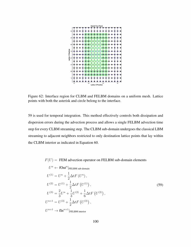
Figure 62: Interface region for CLBM and FELBM domains on a uniform mesh. Latticepoints with both the asterisk and circle belong to the interface.

59 is used for temporal integration. This method effectively controls both dissipation and

dispersion errors during the advection process and allows a single FELBM advection time

step for every CLBM streaming step. The CLBM sub-domain undergoes the classical LBM

streaming to adjacent neighbors restricted to only destination lattice points that lay within

the CLBM interior as indicated in Equation 60.

F (U) = FEM advection operator on FELBM sub-domain elements

Un ← fOutn|FELBM sub-domain

U (1) = Un +1

2∆tF (Un) ,

U (2) = U (1) +1

2∆tF

(U (1)

),

U (3) =2

3Un +

1

3U (2) +

1

6∆tF

(U (2)

),

Un+1 = U (3) +1

2∆tF

(U (3)

),

Un+1 → fInn+1|FELBM interior

(59)

100

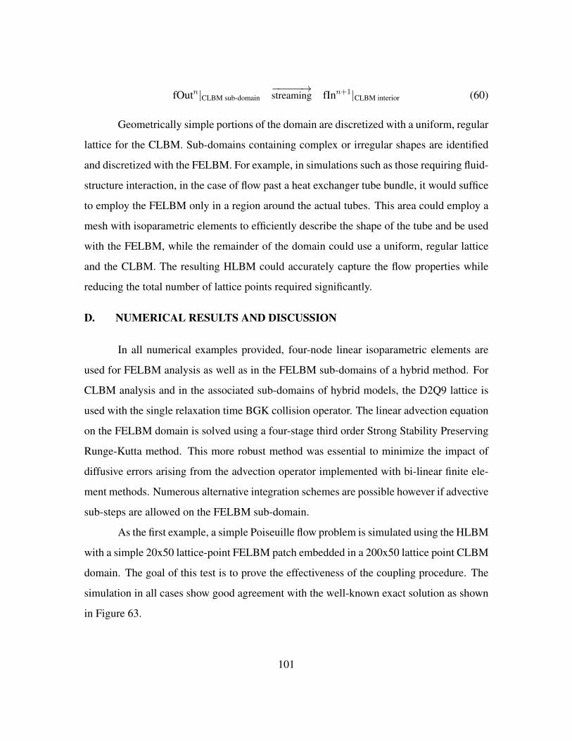
fOutn|CLBM sub-domain−−−−−→streaming fInn+1|CLBM interior (60)

Geometrically simple portions of the domain are discretized with a uniform, regular

lattice for the CLBM. Sub-domains containing complex or irregular shapes are identified

and discretized with the FELBM. For example, in simulations such as those requiring fluid-

structure interaction, in the case of flow past a heat exchanger tube bundle, it would suffice

to employ the FELBM only in a region around the actual tubes. This area could employ a

mesh with isoparametric elements to efficiently describe the shape of the tube and be used

with the FELBM, while the remainder of the domain could use a uniform, regular lattice

and the CLBM. The resulting HLBM could accurately capture the flow properties while

reducing the total number of lattice points required significantly.

D. NUMERICAL RESULTS AND DISCUSSION

In all numerical examples provided, four-node linear isoparametric elements are

used for FELBM analysis as well as in the FELBM sub-domains of a hybrid method. For

CLBM analysis and in the associated sub-domains of hybrid models, the D2Q9 lattice is

used with the single relaxation time BGK collision operator. The linear advection equation

on the FELBM domain is solved using a four-stage third order Strong Stability Preserving

Runge-Kutta method. This more robust method was essential to minimize the impact of

diffusive errors arising from the advection operator implemented with bi-linear finite ele-

ment methods. Numerous alternative integration schemes are possible however if advective

sub-steps are allowed on the FELBM sub-domain.

As the first example, a simple Poiseuille flow problem is simulated using the HLBM

with a simple 20x50 lattice-point FELBM patch embedded in a 200x50 lattice point CLBM

domain. The goal of this test is to prove the effectiveness of the coupling procedure. The

simulation in all cases show good agreement with the well-known exact solution as shown

in Figure 63.

101

Figure 63: Mid-channel normalized velocity profile for Poiseuille flow using CLBM,FELBM and HLBM.

The next numerical test is channel flow with a circular obstacle. The obstacle size

and boundary conditions are selected such that a flow condition corresponding to Reynolds

number of 5 is achieved. The CLBM, FELBM and HLBM methods are employed to simu-

late the fluid flow, but a regular, uniform lattice is maintained in all cases. The obstruction

is placed at L5

where L is the length of the channel.

The last numerical test employs a mixed mesh around the same circular obstacle.

A schematic of the mesh used in the vicinity of the obstacle is shown in Figure 64. As

indicated by the contour plots of both the CLBM and HLBM simulations, both schemes

give results that are in good agreement throughout the computational domain.

102

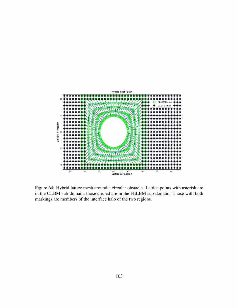
Figure 64: Hybrid lattice mesh around a circular obstacle. Lattice points with asterisk arein the CLBM sub-domain, those circled are in the FELBM sub-domain. Those with bothmarkings are members of the interface halo of the two regions.

103

Figure 65: Normalized velocity contour plot for fluid flow around circular obstacle at Reynolds number = 5 using CLBM

104

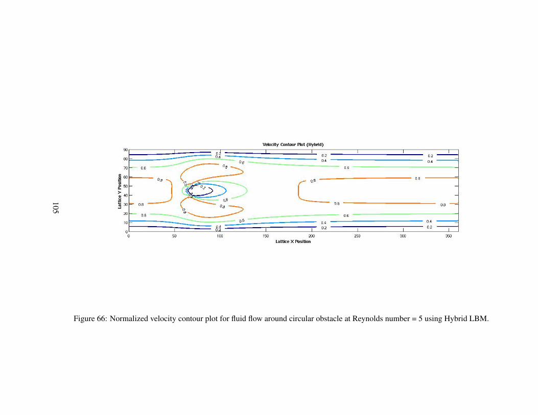
Figure 66: Normalized velocity contour plot for fluid flow around circular obstacle at Reynolds number = 5 using Hybrid LBM.

105

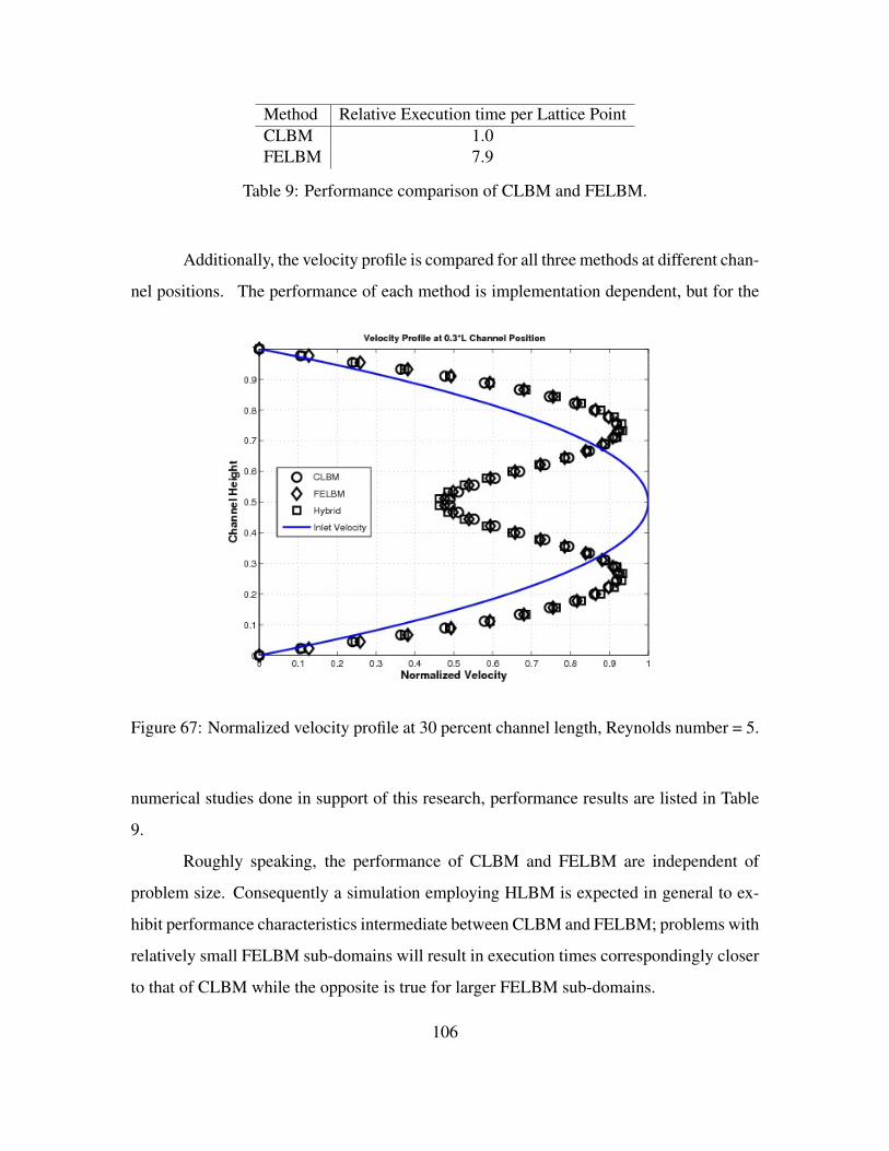
Method Relative Execution time per Lattice PointCLBM 1.0FELBM 7.9

Table 9: Performance comparison of CLBM and FELBM.

Additionally, the velocity profile is compared for all three methods at different chan-

nel positions. The performance of each method is implementation dependent, but for the

Figure 67: Normalized velocity profile at 30 percent channel length, Reynolds number = 5.

numerical studies done in support of this research, performance results are listed in Table

9.

Roughly speaking, the performance of CLBM and FELBM are independent of

problem size. Consequently a simulation employing HLBM is expected in general to ex-

hibit performance characteristics intermediate between CLBM and FELBM; problems with

relatively small FELBM sub-domains will result in execution times correspondingly closer

to that of CLBM while the opposite is true for larger FELBM sub-domains.

106

Figure 68: Normalized velocity profile at 60 percent channel length, Reynolds number = 5.

Problems of practical interest introduce non-trivial complexities into this perfor-

mance analysis. Applications using HLBM as an alternative to CLBM are expected to

utilize significantly fewer lattice points and thus require significantly less time. In addi-

tion to reducing required run-time for a given simulation, this feature will allow for a more

detailed simulations to be conducted on a workstation-size computer.

As an illustration of the potential benefit for curved or irregular boundaries, consider

the discretization of the surface of the circular obstruction considered in this dissertation in

Figure 69. The HLBM code used for this analysis required 10,210 lattice points for both

sub-domains. Comparably realistic depiction of the curved boundary requires significantly

more lattice points in a uniform, regular lattice over the entire domain.

107

Figure 69: Schematic Hybrid Lattice on regular domain. Assignment following streamingin the CLBM domain and advection in the FELBM domain is only made to the interiorof each respective sub-domain. Data drawn from the lattice points on the halo facilitatescommunication between each sub-domain.

108

VII. LBM FOR MULTI-COMPONENT FLUIDS

The results and associated discussion presented thus far in this work have focused

solely on single-phase, single-component fluid models. One of the strengths of LBM lies

in its natural amenability to multicomponent fluids. In this chapter, the main features of

the leading multi-component LBM fluid models will be outlined and example applications

will be presented for two-dimensional single-phase multi-component flows.

A. MULTI-COMPONENT FLUID MODELS

There are four main multi-component fluid models in LBM theory. The color-

fluid model [88], the inter-particle-potential model [89], the free-energy model [90] and

the mean-field theory model [91]. The methods can all be compared based on the way in

which the surface tension of the component interface is taken into account in the evolution

of the particle distribution functions and how the location of this interface is determined.

Excellent surveys of multi-component fluid flows are provided in [14]-[16]. In this work,

the inter-particle potential model is used, so this method will be discussed in greater detail;

the other methods will only be briefly reviewed.

1. Color-Fluid Model

The color fluid model was introduced with the publication of [88] to allow the sim-

ulation of immiscible binary fluids in two dimensions. It is based on the two-component

cellular-automata model introduced in [92] and modified for use with LBM. The method

is referred to as the color-fluid model due to the convention of referring to the binary fluid

mixture in terms of “red” particles and “blue” particles. The LBM is carried out for each

fluid species and the surface-tension effect on particle distributions is emulated with an

additional perturbation term appended to the collision operator. This term, in combination

with a “recoloring” step—a correction based on the local color gradient that forces to shift

to a direction leading to other like-colored particles—locally places the interface as well

109

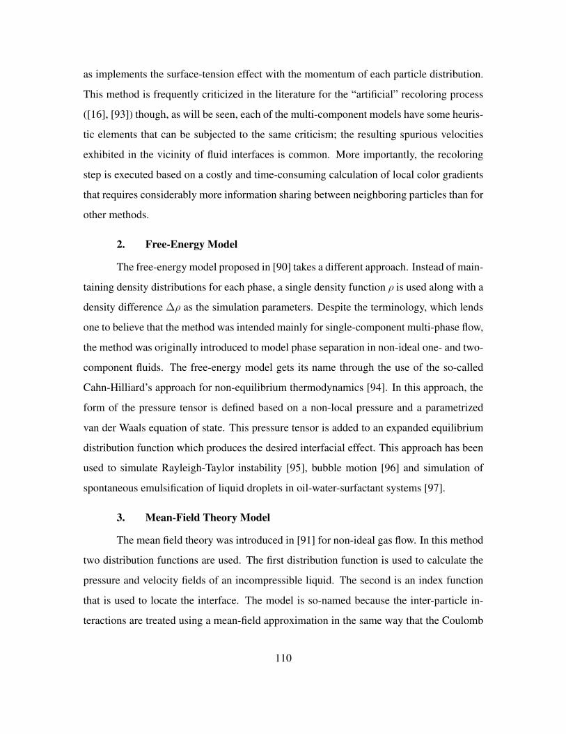
as implements the surface-tension effect with the momentum of each particle distribution.

This method is frequently criticized in the literature for the “artificial” recoloring process

([16], [93]) though, as will be seen, each of the multi-component models have some heuris-

tic elements that can be subjected to the same criticism; the resulting spurious velocities

exhibited in the vicinity of fluid interfaces is common. More importantly, the recoloring

step is executed based on a costly and time-consuming calculation of local color gradients

that requires considerably more information sharing between neighboring particles than for

other methods.

2. Free-Energy Model

The free-energy model proposed in [90] takes a different approach. Instead of main-

taining density distributions for each phase, a single density function ρ is used along with a

density difference ∆ρ as the simulation parameters. Despite the terminology, which lends

one to believe that the method was intended mainly for single-component multi-phase flow,

the method was originally introduced to model phase separation in non-ideal one- and two-

component fluids. The free-energy model gets its name through the use of the so-called

Cahn-Hilliard’s approach for non-equilibrium thermodynamics [94]. In this approach, the

form of the pressure tensor is defined based on a non-local pressure and a parametrized

van der Waals equation of state. This pressure tensor is added to an expanded equilibrium

distribution function which produces the desired interfacial effect. This approach has been

used to simulate Rayleigh-Taylor instability [95], bubble motion [96] and simulation of

spontaneous emulsification of liquid droplets in oil-water-surfactant systems [97].

3. Mean-Field Theory Model

The mean field theory was introduced in [91] for non-ideal gas flow. In this method

two distribution functions are used. The first distribution function is used to calculate the

pressure and velocity fields of an incompressible liquid. The second is an index function

that is used to locate the interface. The model is so-named because the inter-particle in-

teractions are treated using a mean-field approximation in the same way that the Coulomb

110

interaction among charged particles of a plasma is treated in the Vlasov equation [98],

[99]. As several authors have pointed out, this approach is similar to the traditional CFD

methods for interface capturing and is the LBM analogy to the level-set [100] and volume

of fluid methods [101]. This model has been successfully used to model Rayleigh-Taylor

and Kelvin-Helmholtz instabilities [102], [103] with non-ideal dense fluids among other

applications.

4. Inter-Particle Potential Model

The inter-particle potential model was proposed in [89] as a simple means to simu-

late multi-phase and multi-component fluids. The fundamental idea is that the surface ten-

sion effects which conventional CFD methods attempt to account for in multi-component

flows is microscopic in origin; the same effect could be incorporated into the LBM via

these same inter-particle potential forces. In this model, only the nearest neighbor particle

densities are considered and they are introduced as follows in Equation 61:

F (x, t) = −Gψ (x, t)

q−1∑α=1

wαψ (x + eα∆t, t) eα. (61)

where x is particle position, G is a parameter indicating interaction strength, ψ(x, t) is a

function describing the interaction potential, wα is the lattice weight for direction α and

eα is the corresponding lattice velocity. The form of the potential function can be varied

to obtain the desired inter-particle potential behavior. For multiphase flow, ψ is commonly

expressed as in Equation 62:

ψ (ρ) = ψ0 exp

(−ρ0

ρ

). (62)

where ψ0 and ρ0 are arbitrary parameters selected so as to achieve appropriate dynamics

for a selected fluid system. The multicomponent fluids systems used in this work are only

qualitatively correlated with real fluid systems in that only density and viscosity are set and

scaled consistently with the LBM. The parameter G is set so as to generate a desired level

of immiscibility while maintaining simulation stability. The potential function is set as

111

Figure 70: Illustration of inter-particle forces in the nearest neighborhood of a lattice point.

ψ (x, t) = ρ (x, t). Notice that Equation 61 specifies a weighted summation of the value of

ψ for each lattice position in the neighborhood of a given lattice particle. This is illustrated

schematically in Figure 70.

B. IMMISCIBLE MULTI-COMPONENT LBM PROCEDURES

The basic LBM process with multiple components is similar in most ways to that

used for single-component systems as illustrated in Figure 10. The obvious difference is

that there are now two sets of distribution functions; as before fα and for a second com-

ponent that will conventionally be referred to as gα. Along with the physical domain, both

fluids are scaled according to the scaling rules discussed in Chapter II. A second difference

is that, as discussed in the preceding paragraphs, the inter-particle force must be calculated

in accordance with Equation 61 and incorporated into the calculation of macroscopic ve-

locity used for computing f eq and geq using Equation 35 and Equation 36. The biggest and

most fundamental difference is the need to structure the computations so as to account for

112

the fact that, due to the desired macroscopic dynamic evolution of the system, some lattice

sites will have zero density for one or the other component; only the interfaces will have a

significant mixture.

1. Time Stepping

In order to be as explicit as possible, the immiscible multicomponent LBM time-

step for fluid lattice points is carried out for this work was implemented as follows:

1. Compute macroscopic density of each fluid:

ρf =

q−1∑α=0

fα

ρg =

q−1∑α=0

gα

2. Compute macroscopic momentum of each fluid:

ρfuf =

q−1∑α=0

eαfα

ρgug =

q−1∑α=0

eαgα

3. Compute a weighted combined macroscopic density and velocity:

ρω = ρfωf + ρgωg

u =ρfufωf + ρgugωg

ρω

where we recall ω = 1τ.

113

4. Compute inter-particle force using Equation 61 setting G to a constant,

and ψ (x, t) = ρ:

Ff = −Gρgq−1∑α=1

wαρg (x + eα∆t, t)

Fg = −Gρfq−1∑α=1

wαρf (x + eα∆t, t)

5. Apply these inter-particle forces as momentum inputs to each respective

lattice population:

ueqf = uf − τfFf

ueqg = ug − τgFg

6. Complete the usual LBGK collision and streaming steps using ueqf and ueqg

and corresponding macroscopic density for computation of f eq and geq

accordingly.

2. Boundary Conditions

For this work, three types of boundary conditions have so far been used: periodic

boundaries, bounce-back boundaries and moving boundaries. The bounce-back and pe-

riodic boundary conditions for multi-component LBM is the same as for ordinary LBM.

Solid nodes bounce-back by swapping the density distribution function across opposite

directions as illustrated in Figure 5 in Chapter II. It should be noted that the density dis-

tribution values resident on solid nodes do not contribute to the nearest-neighbor force

calculation given in Equation 61. The moving boundary condition is employed in the same

way as with single-component fluid models using the weighted macroscopic velocity given

in step 3 of the above procedure.

114

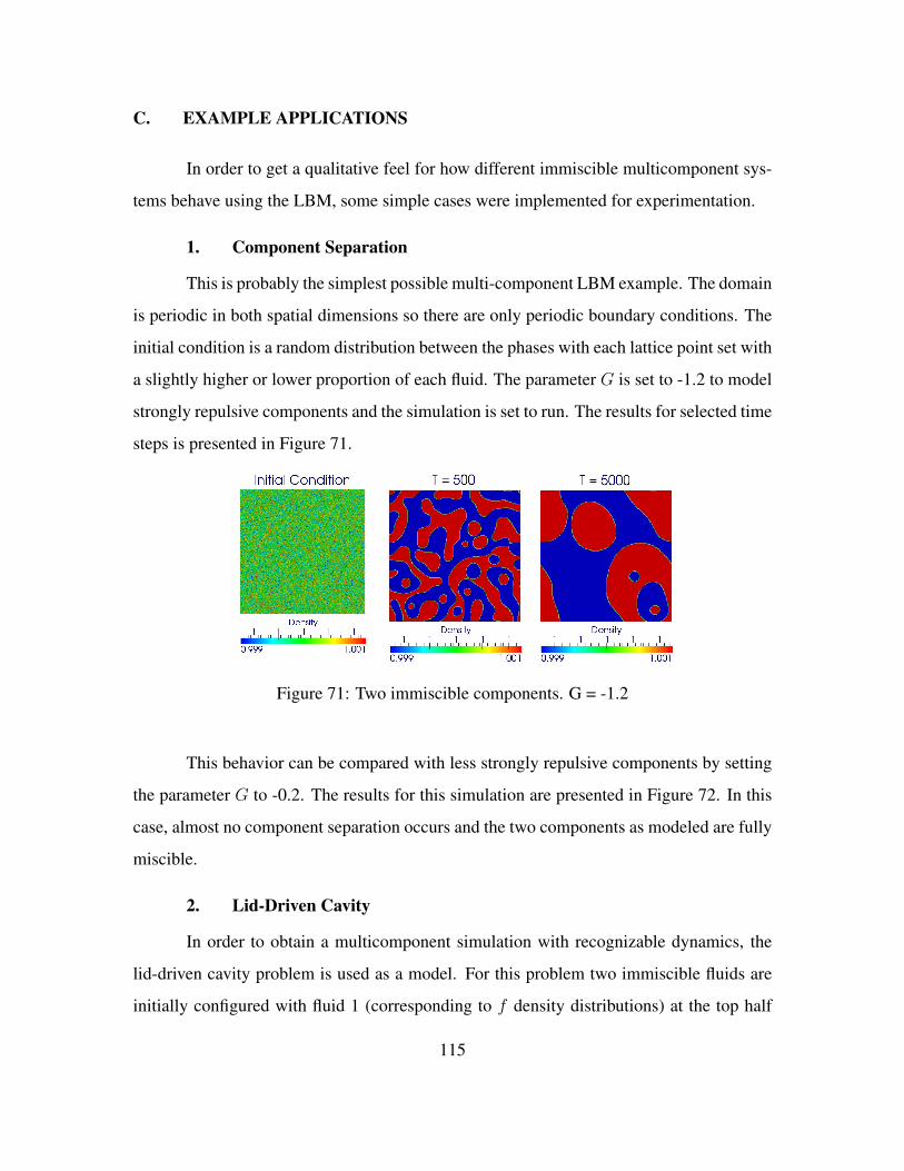
C. EXAMPLE APPLICATIONS

In order to get a qualitative feel for how different immiscible multicomponent sys-

tems behave using the LBM, some simple cases were implemented for experimentation.

1. Component Separation

This is probably the simplest possible multi-component LBM example. The domain

is periodic in both spatial dimensions so there are only periodic boundary conditions. The

initial condition is a random distribution between the phases with each lattice point set with

a slightly higher or lower proportion of each fluid. The parameter G is set to -1.2 to model

strongly repulsive components and the simulation is set to run. The results for selected time

steps is presented in Figure 71.

Figure 71: Two immiscible components. G = -1.2

This behavior can be compared with less strongly repulsive components by setting

the parameter G to -0.2. The results for this simulation are presented in Figure 72. In this

case, almost no component separation occurs and the two components as modeled are fully

miscible.

2. Lid-Driven Cavity

In order to obtain a multicomponent simulation with recognizable dynamics, the

lid-driven cavity problem is used as a model. For this problem two immiscible fluids are

initially configured with fluid 1 (corresponding to f density distributions) at the top half

115

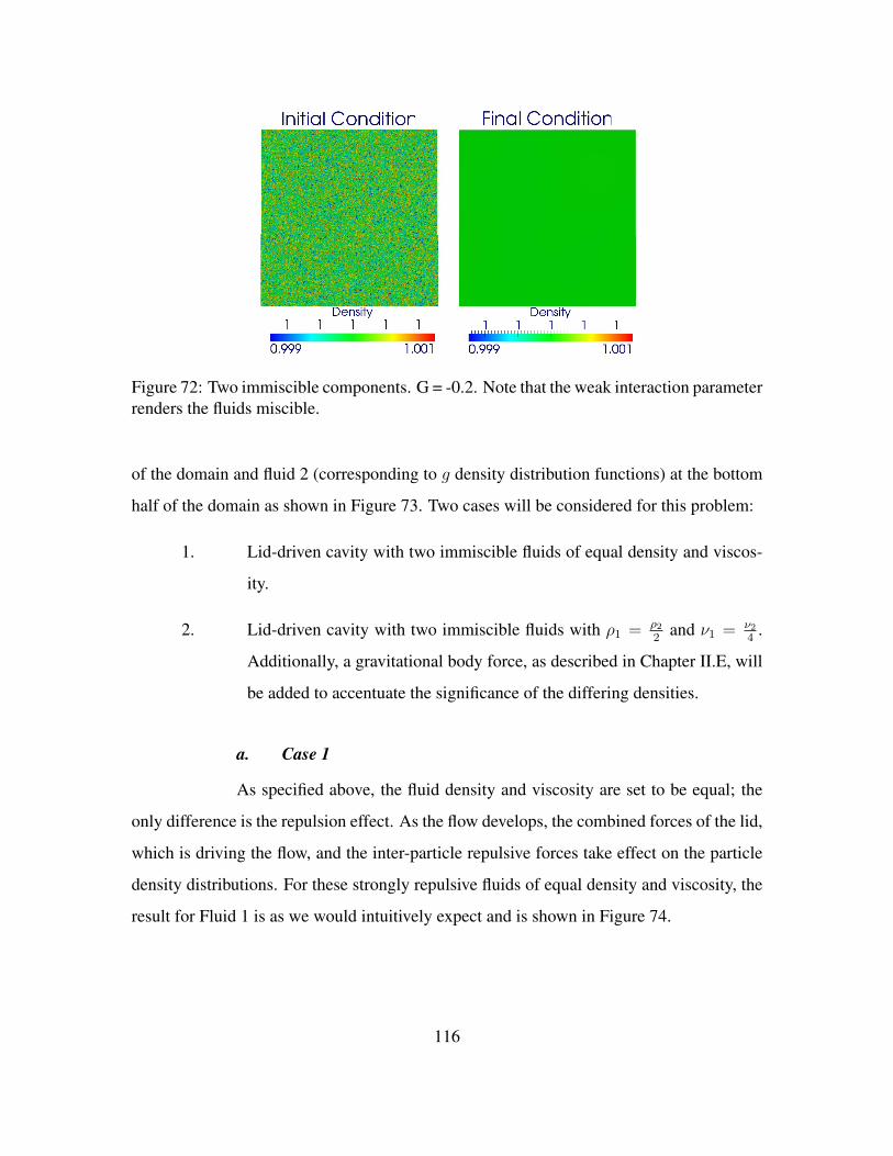
Figure 72: Two immiscible components. G = -0.2. Note that the weak interaction parameterrenders the fluids miscible.

of the domain and fluid 2 (corresponding to g density distribution functions) at the bottom

half of the domain as shown in Figure 73. Two cases will be considered for this problem:

1. Lid-driven cavity with two immiscible fluids of equal density and viscos-

ity.

2. Lid-driven cavity with two immiscible fluids with ρ1 = ρ22

and ν1 = ν24

.

Additionally, a gravitational body force, as described in Chapter II.E, will

be added to accentuate the significance of the differing densities.

a. Case 1

As specified above, the fluid density and viscosity are set to be equal; the

only difference is the repulsion effect. As the flow develops, the combined forces of the lid,

which is driving the flow, and the inter-particle repulsive forces take effect on the particle

density distributions. For these strongly repulsive fluids of equal density and viscosity, the

result for Fluid 1 is as we would intuitively expect and is shown in Figure 74.

116

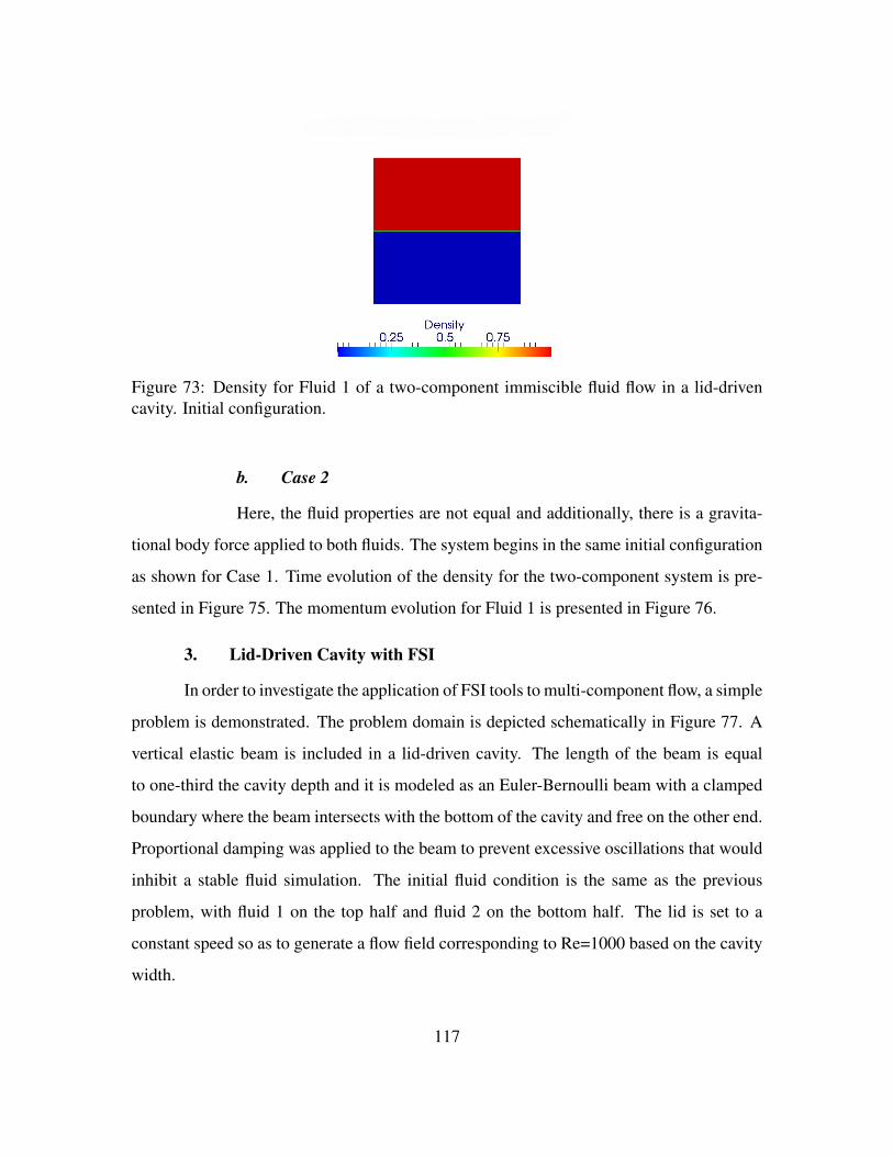
Figure 73: Density for Fluid 1 of a two-component immiscible fluid flow in a lid-drivencavity. Initial configuration.

b. Case 2

Here, the fluid properties are not equal and additionally, there is a gravita-

tional body force applied to both fluids. The system begins in the same initial configuration

as shown for Case 1. Time evolution of the density for the two-component system is pre-

sented in Figure 75. The momentum evolution for Fluid 1 is presented in Figure 76.

3. Lid-Driven Cavity with FSI

In order to investigate the application of FSI tools to multi-component flow, a simple

problem is demonstrated. The problem domain is depicted schematically in Figure 77. A

vertical elastic beam is included in a lid-driven cavity. The length of the beam is equal

to one-third the cavity depth and it is modeled as an Euler-Bernoulli beam with a clamped

boundary where the beam intersects with the bottom of the cavity and free on the other end.

Proportional damping was applied to the beam to prevent excessive oscillations that would

inhibit a stable fluid simulation. The initial fluid condition is the same as the previous

problem, with fluid 1 on the top half and fluid 2 on the bottom half. The lid is set to a

constant speed so as to generate a flow field corresponding to Re=1000 based on the cavity

width.

117

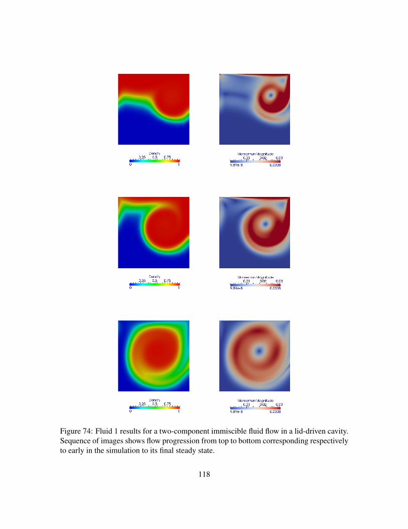
Figure 74: Fluid 1 results for a two-component immiscible fluid flow in a lid-driven cavity.Sequence of images shows flow progression from top to bottom corresponding respectivelyto early in the simulation to its final steady state.

118

0.25 Density

0.5 0.75 I '

Figure 75: Fluid 1 results for a two-component immiscible fluid flow in a lid driven cavity.The higher viscosity and density of fluid 2 results in its confinement in the bottom-half ofthe cavity domain.

Figure 76: Fluid 1 results for a two-component immiscible fluid flow in a lid driven cavity.The higher viscosity and density of fluid 2 results in its confinement in the bottom-half ofthe cavity domain.

119

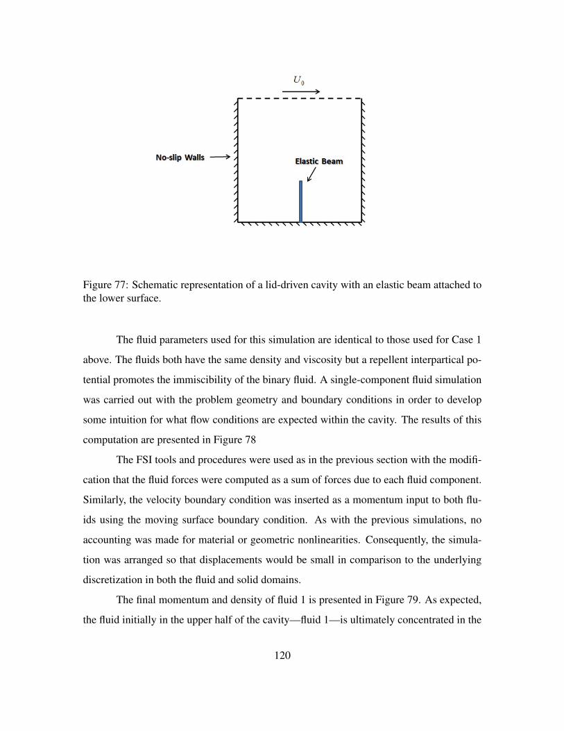
Figure 77: Schematic representation of a lid-driven cavity with an elastic beam attached tothe lower surface.

The fluid parameters used for this simulation are identical to those used for Case 1

above. The fluids both have the same density and viscosity but a repellent interpartical po-

tential promotes the immiscibility of the binary fluid. A single-component fluid simulation

was carried out with the problem geometry and boundary conditions in order to develop

some intuition for what flow conditions are expected within the cavity. The results of this

computation are presented in Figure 78

The FSI tools and procedures were used as in the previous section with the modifi-

cation that the fluid forces were computed as a sum of forces due to each fluid component.

Similarly, the velocity boundary condition was inserted as a momentum input to both flu-

ids using the moving surface boundary condition. As with the previous simulations, no

accounting was made for material or geometric nonlinearities. Consequently, the simula-

tion was arranged so that displacements would be small in comparison to the underlying

discretization in both the fluid and solid domains.

The final momentum and density of fluid 1 is presented in Figure 79. As expected,

the fluid initially in the upper half of the cavity—fluid 1—is ultimately concentrated in the

120

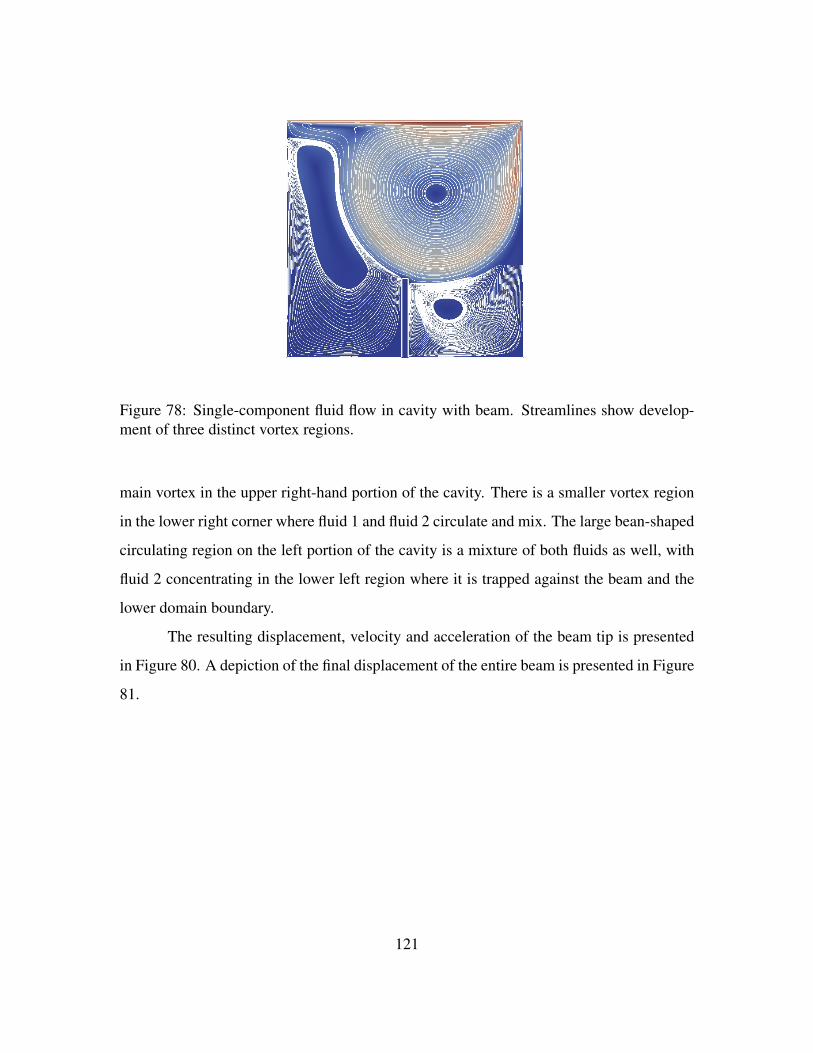
Figure 78: Single-component fluid flow in cavity with beam. Streamlines show develop-ment of three distinct vortex regions.

main vortex in the upper right-hand portion of the cavity. There is a smaller vortex region

in the lower right corner where fluid 1 and fluid 2 circulate and mix. The large bean-shaped

circulating region on the left portion of the cavity is a mixture of both fluids as well, with

fluid 2 concentrating in the lower left region where it is trapped against the beam and the

lower domain boundary.

The resulting displacement, velocity and acceleration of the beam tip is presented

in Figure 80. A depiction of the final displacement of the entire beam is presented in Figure

81.

121

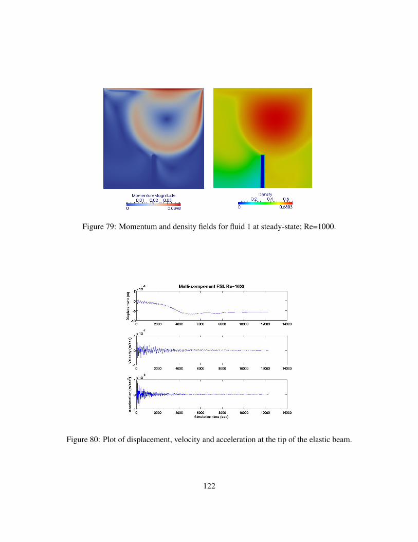
Figure 79: Momentum and density fields for fluid 1 at steady-state; Re=1000.

Figure 80: Plot of displacement, velocity and acceleration at the tip of the elastic beam.

122

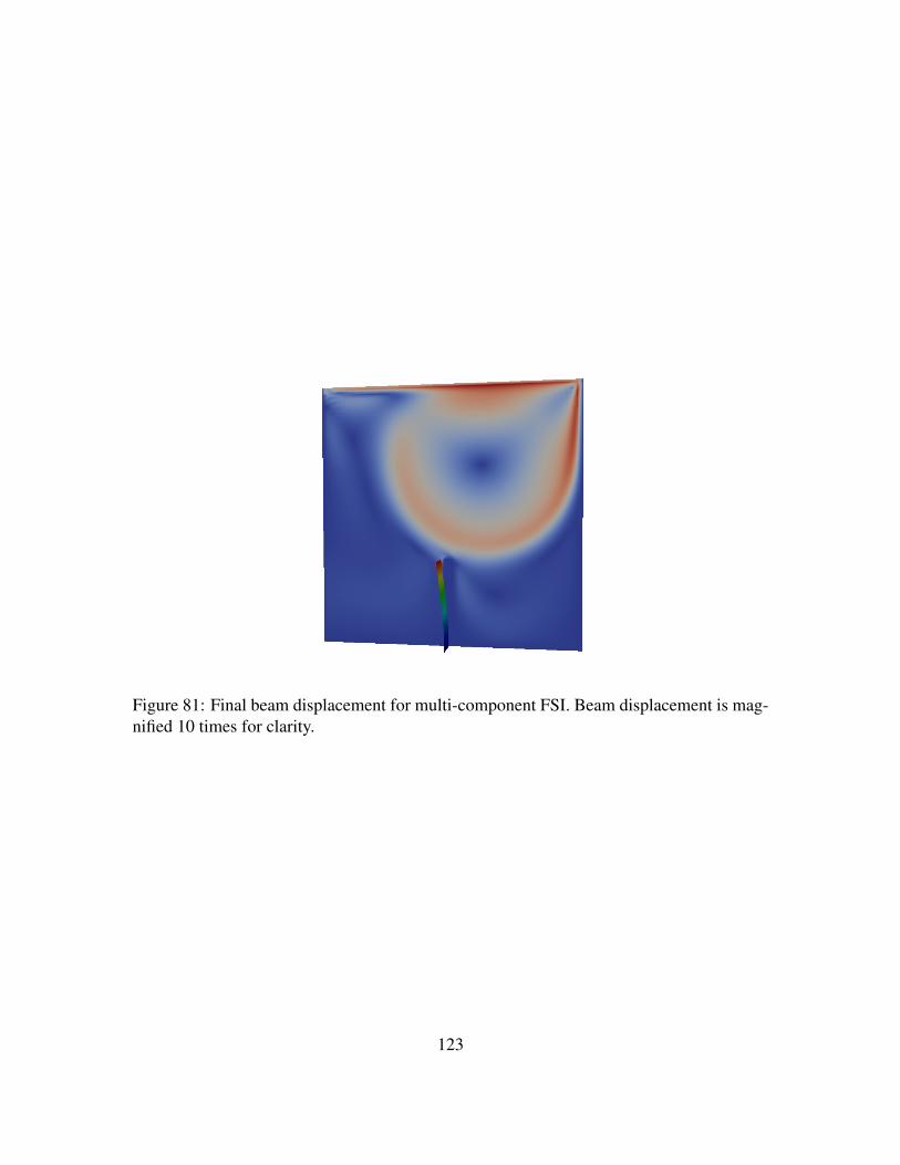
Figure 81: Final beam displacement for multi-component FSI. Beam displacement is mag-nified 10 times for clarity.

123


124

VIII. CONCLUSIONS AND FUTURE WORK

A. CONCLUSIONS

The primary objective of this thesis is to investigate the use of LBM to model vis-

cous incompressible flow and model the interactions that flow has with surrounding struc-

tures. In accomplishing this goal, several outcomes have been achieved:

1. A body of software has been developed to allow LBM modeling of single-

component incompressible flow in two and three dimensions.

(a) This software was validated against a selection of two- and three-

dimensional benchmark problems and shown to accurately model

low and moderate Reynolds number fluid flows

(b) It was shown that the expected quadratic convergence properties

of LBM can be lost for single-precision computations and a new

mixed-precision implementation was demonstrated to extend the

range of quadratic convergence at less computational expense than

carrying out computations in full double precision.

(c) The software performance was compared to other single-GPU

implementations reported in the recent literature and it was shown

that the implementation presented for this thesis outperforms all

others over certain problem sizes and is highly competitive for all

problem sizes.

2. The LBM software tools were extended to incorporate structural interac-

tions thus allowing FSI simulations.

(a) FSI simulations were demonstrated for both two- and three-dimensional

single-component fluid flow problems.

125

(b) A novel heterogeneous parallel implementation was described

where task-level parallelism inherent in the FSI problem is parceled

among both the CPU and GPU on a single workstation. It was

shown that by decomposing the problem domain that performance

can be improved by over 23 percent for some problems.

(c) A simple two-dimensional FSI simulation was presented for multi-

component fluid flows.

3. A novel method for combining CLBM and FELBM into a HBLM was de-

veloped. This allows the efficient description of curved domain boundaries

while minimizing the computational expense of FELBM.

B. FUTURE WORK

Much work remains to be done for future research in LBM for fluid flows. For

single-component fluid flows, the software tools presented in this work only accommodate

flows for Reynolds number up to approximately 10,000. Current research in entropic and

thermal LBM along with single and multi-parameter turbulence models can be incorporated

to extend the range of simulation up through at least the range of incompressible fluid

flow. Further research needs to be done to include some capability for compressible flow

modeling. Accomplishment of these goals will greatly expand the range of applicability of

the LBM models presented here and open the door to a multitude of interesting research

applications.

The multi-component fluid flow modeling capability is also in need of much work.

Current implementations are restrictive in the range of fluid density and viscosity ratios

that can be stably simulated. Additionally, more physical fidelity is required in the inter-

particle potential modeling to allow predictive rather than merely qualitative simulations to

be conducted.

For successful application of improved LBM models to more realistic problem

types, the need exists to further extend the performance and scalability of the software

126

tools. As implemented for this work, excellent performance was obtained for software run

on a single GPU or a small number of GPUs attached to a single workstation. The scal-

ing achieved for multiple GPUs over multiple platforms was less well developed for this

work. To accommodate future scaling, improved partitioning strategies must be included

and incorporated into the software platform in a way that allows efficient scaling to an ar-

bitrarily large set of computational resources. Additionally, software components such as

solid modelers and mesh generators must be adopted and interfaced with existing tools to

assist with LBM problem formulation and setup.

In order to employ lattice Boltzmann fluid models for future FSI research on more

physically relevant problems, extensive work is also required for both the structural models

as well as the LBM computational routines. Of highest priority for the structural model is

the need to incorporate geometric and material non-linearity into the dynamic models. FSI

problems of practical interest involve deformations that are not small and strains that are

large. Consequently, linear elastic structural dynamics models are overly restrictive in the

range of problems for which they will provide a satisfactory answer. Future research efforts

will be directed towards meeting this need with a full range of non-linear material constitu-

tive models and FEM technology to accommodate moving and deforming meshes. On the

fluid modeling front, it is imperative that extensions be developed to admit moving solid

boundaries that displace over an arbitrary number of lattice points. Methods must be imple-

mented to properly initialize and update lattice points that are either entering or emerging

a non-fluid domain. Alternately, non-classical LBM formulations such as FELBM and

HLBM must be further developed so that both the fluid and solid domain can be consis-

tently described in a Lagrangian manner within a given FSI simulation over a more broad

range of problems.

127


128

LIST OF REFERENCES

[1] Z. Guo and T. S. Zhao, “Lattice Boltzmann model for incompressible flows throughporous media,” Phys. Rev. E, vol. 66, p. 036304, Sep 2002.

[2] G. H. Tang, W. Q. Tao, and Y. L. He, “Gas slippage effect on microscale porous flowusing the lattice Boltzmann method,” Phys. Rev. E, vol. 72, p. 056301, Nov 2005.

[3] M. Yoshino and T. Inamuro, “Lattice Boltzmann simulations for flow and heat/masstransfer problems in a three-dimensional porous structure,” International Journal forNumerical Methods in Fluids, vol. 43, no. 2, pp. 183–198, 2003.

[4] T. Inamuro, T. Ogata, S. Tajima, and N. Konishi, “A lattice Boltzmann method forincompressible two-phase flows with large density differences,” Journal of Compu-tational Physics, vol. 198, no. 2, pp. 628 – 644, 2004.

[5] G. Hzi, A. R. Imre, G. Mayer, and I. Farkas, “Lattice Boltzmann methods for two-phase flow modeling,” Annals of Nuclear Energy, vol. 29, no. 12, pp. 1421–1453,2002.

[6] Y. Yan and Y. Zu, “A lattice Boltzmann method for incompressible two-phaseflows on partial wetting surface with large density ratio,” Journal of ComputationalPhysics, vol. 227, no. 1, pp. 763–775, 2007.

[7] G. Breyiannis and D. Valougeorgis, “Lattice kinetic simulations in three-dimensional magnetohydrodynamics,” Phys. Rev. E, vol. 69, p. 065702, Jun 2004.

[8] M. Pattison, K. Premnath, N. Morley, and M. Abdou, “Progress in lattice Boltzmannmethods for magnetohydrodynamic flows relevant to fusion applications,” FusionEngineering and Design, vol. 83, no. 4, pp. 557–572, 2008.

[9] J. Carter and L. Oliker, “Performance evaluation of lattice-Boltzmann magnetohy-drodynamics simulations on modern parallel vector systems,” in High PerformanceComputing on Vector Systems (M. Resch, T. Bnisch, K. Benkert, W. Bez, T. Furui,and Y. Seo, eds.), pp. 41–50, Springer Berlin Heidelberg, 2006.

[10] B. H. Elton, “A lattice Boltzmann method for a two-dimensional viscous Burgersequation: Computational results.,” in Supercomputing, pp. 242–252, 1991.

[11] G. Yan and J. Zhang, “A higher-order moment method of the lattice Boltz-mann model for the Korteweg-de Vries equation,” Math. Comput. Simul., vol. 79,pp. 1554–1565, January 2009.

[12] N. S. Martys, “Improved approximation of the Brinkman equation using a latticeBoltzmann method,” Phys. Fluids, vol. 13, no. 6, pp. 1807–1810, 2001.

129

[13] L. Zhong, S. Feng, P. Dong, and S. Gao, “Lattice Boltzmann schemes for the non-linear Schrodinger equation,” Phys. Rev. E, vol. 74, p. 036704, Sep 2006.

[14] S. Chen and G. D. Doolen, “Lattice Boltzmann method for fluid flows,” AnnualReview of Fluid Mechanics, vol. 30, no. 1, pp. 329–364, 1998.

[15] C. K. Aidun and J. R. Clausen, “Lattice-Boltzmann method for complex flows,”Annual Review of Fluid Mechanics, vol. 42, no. 1, pp. 439–472, 2010.

[16] R. Nourgaliev, T. Dinh, T. Theofanous, and D. Joseph, “The lattice Boltzmann equa-tion method: theoretical interpretation, numerics and implications,” InternationalJournal of Multiphase Flow, vol. 29, pp. 117–169, JAN 2003.

[17] S. Wolfram, “Cellular automaton fluids 1: Basic theory,” Journal of StatisticalPhysics, vol. 45, pp. 471–526, 1986.

[18] U. Frisch, B. Hasslacher, and Y. Pomeau, “Lattice-gas automata for the Navier-Stokes equation,” Phys. Rev. Lett., vol. 56, pp. 1505–1508, Apr 1986.

[19] S. Wolfram, Theory and Applications of Cellular Automata. Singapore: World Sci-entific Publication, 1986.

[20] D. Helbing and M. Schreckenberg, “Cellular automata simulating experimentalproperties of traffic flow,” Phys. Rev. E, vol. 59, pp. R2505–R2508, Mar 1999.

[21] J. Molofsky, “Population dynamics and pattern formation in theoretical popula-tions,” Ecology, vol. 75, no. 1, pp. 30–39, 1994.

[22] J. Huang, G. Narkounskaia, and D. L. Turcotte, “A cellular-automata, slider-blockmodel for earthquakes ii. demonstration of self-organized criticality for a 2-d sys-tem,” Geophysical Journal International, vol. 111, no. 2, pp. 259–269, 1992.

[23] G. R. McNamara and G. Zanetti, “Use of the Boltzmann equation to simulate lattice-gas automata,” Phys. Rev. Lett., vol. 61, pp. 2332–2335, Nov 1988.

[24] D. d’Humıeres, “Generalized lattice-Boltzmann equations,” in Rarefied gas dynam-ics - Theory and simulations; Proceedings of the 18th International Symposium onRarefied Gas Dynamics, (University of British Columbia, Vancouver, Canada), July1992.

[25] P. Lallemand and L.-S. Luo, “Theory of the lattice Boltzmann method: Disper-sion, dissipation, isotropy, Galilean invariance, and stability,” Phys. Rev. E, vol. 61,pp. 6546–6562, Jun 2000.

[26] D. P. Ziegler, “Boundary conditions for lattice Boltzmann simulations,” Journal ofStatistical Physics, vol. 71, pp. 1171–1177, 1993.

130

[27] R. Mei, W. Shyy, D. Yu, and L.-S. Luo, “Lattice Boltzmann method for 3-D flowswith curved boundary,” Journal of Computational Physics, vol. 161, no. 2, pp. 680– 699, 2000.

[28] Y. W. Kwon, “Coupling of lattice Boltzmann and finite element methods for fluid-structure interaction application,” Journal of Pressure Vessel Technology, vol. 130,no. 1, p. 011302, 2008.

[29] J. Latt, B. Chopard, O. Malaspinas, M. Deville, and A. Michler, “Straight velocityboundaries in the lattice Boltzmann method,” Phys. Rev. E, vol. 77, p. 056703, May2008.

[30] Q. Zou and X. He, “On pressure and velocity flow boundary conditions and bounce-back for the lattice Boltzmann BGK model,” Contributions to Mineralogy andPetrology, pp. 11001–+, Nov. 1996.

[31] J. Latt, Hydrodynamic limit of lattice Boltzmann equations. PhD dissertation, Uni-versity of Geneva, 2007.

[32] Q. Zou and X. He, “On pressure and velocity boundary conditions for the latticeBoltzmann BGK model,” Phys. Fluids, vol. 9, June 1997.

[33] D. Yu, R. Mei, L.-S. Luo, and W. Shyy, “Viscous flow computations with the methodof lattice Boltzmann equation,” Progress in Aerospace Sciences, vol. 39, no. 5,pp. 329 – 367, 2003.

[34] B. F. Armaly, F. Durst, and J. C. F. Pereira, “Experimental and theoretical investiga-tion of backward-facing step flow,” Journal of Fluid Mechanics, vol. 127, pp. 473–496, 1983.

[35] U. Ghia, K. Ghia, and C. Shin, “High-Re solutions for incompressible flow usingthe Navier-Stokes equations and a multigrid method,” Journal of ComputationalPhysics, vol. 48, no. 3, pp. 387 – 411, 1982.

[36] O. Botella and R. Peyret, “Benchmark spectral results on the lid-driven cavity flow,”Computers and Fluids, vol. 27, no. 4, pp. 421 – 433, 1998.

[37] C.-H. Bruneau and M. Saad, “The 2D lid-driven cavity problem revisited,” Comput-ers and Fluids, vol. 35, no. 3, pp. 326 – 348, 2006.

[38] H. Zhou, G. Mo, F. Wu, J. Zhao, M. Rui, and K. Cen, “GPU implementation oflattice Boltzmann method for flows with curved boundaries,” Computer Methods inApplied Mechanics and Engineering, vol. 225228, no. 0, pp. 65 – 73, 2012.

[39] W. Li, X. Wei, and A. Kaufman, “Implementing lattice Boltzmann computa-tion on graphics hardware,” The Visual Computer, vol. 19, pp. 444–456, 2003.10.1007/s00371-003-0210-6.

131

[40] D. Calhoun, “A Cartesian grid method for solving the two-dimensionalstreamfunction-vorticity equations in irregular regions,” Journal of ComputationalPhysics, vol. 176, no. 2, pp. 231 – 275, 2002.

[41] S. Xu and Z. J. Wang, “An immersed interface method for simulating the interactionof a fluid with moving boundaries,” Journal of Computational Physics, vol. 216,no. 2, pp. 454 – 493, 2006.

[42] D. Russell and Z. J. Wang, “A Cartesian grid method for modeling multiple mov-ing objects in 2D incompressible viscous flow,” Journal of Computational Physics,vol. 191, no. 1, pp. 177 – 205, 2003.

[43] L. Ong and J. Wallace, “The velocity field of the turbulent very near wakeof a circular cylinder,” Experiments in Fluids, vol. 20, pp. 441–453, 1996.10.1007/BF00189383.

[44] A. L. E. Silva, A. Silveira-Neto, and J. Damasceno, “Numerical simulation of two-dimensional flows over a circular cylinder using the immersed boundary method,”Journal of Computational Physics, vol. 189, no. 2, pp. 351 – 370, 2003.

[45] C. Obrecht, F. Kuznik, B. Tourancheau, and J.-J. Roux, “A new approach to the lat-tice Boltzmann method for graphics processing units,” Computers and Mathematicswith Applications, vol. 61, no. 12, pp. 3628 – 3638, 2011.

[46] J. Tolke, “Implementation of a lattice Boltzmann kernel using the compute unifieddevice architecture developed by NVIDIA,” Comput. Vis. Sci., vol. 13, pp. 29–39,Nov. 2009.

[47] P. Bailey, J. Myre, S. Walsh, D. Lilja, and M. Saar, “Accelerating lattice Boltzmannfluid flow simulations using graphics processors,” in Parallel Processing, 2009.ICPP ’09. International Conference on, pp. 550 –557, sept. 2009.

[48] M. Bernaschi, M. Fatica, S. Melchionna, S. Succi, and E. Kaxiras, “A flexible high-performance lattice Boltzmann GPU code for the simulations of fluid flows in com-plex geometries,” Concurr. Comput. : Pract. Exper., vol. 22, pp. 1–14, Jan. 2010.

[49] P. Rinaldi, E. Dari, M. Vnere, and A. Clausse, “A lattice-Boltzmann solver for 3Dfluid simulation on GPU,” Simulation Modelling Practice and Theory, vol. 25, no. 0,pp. 163 – 171, 2012.

[50] M. Astorino, J. B. Sagredo, and A. Quarteroni, “A modular lattice Boltzmann solverfor GPU computing processors,” Tech. Rep. MATHICSE-TR-06-2011, Mathemat-ics Institute of Computational Science and Engineering, Lucerne, Switzerland, July2011.

132

[51] K. Mattila, J. Hyvluoma, J. Timonen, and T. Rossi, “Comparison of implementationsof the lattice-Boltzmann method,” Computers and Mathematics with Applications,vol. 55, no. 7, pp. 1514 – 1524, 2008.

[52] NVIDIA Corporation, NVIDIA CUDA C Programming Guide, 4.2 ed., April 2012.

[53] V. W. Lee, C. Kim, J. Chhugani, M. Deisher, D. Kim, A. D. Nguyen, N. Satish,M. Smelyanskiy, S. Chennupaty, P. Hammarlund, R. Singhal, and P. Dubey, “De-bunking the 100x GPU vs. CPU myth: an evaluation of throughput computing onCPU and GPU,” SIGARCH Comput. Archit. News, vol. 38, pp. 451–460, June 2010.

[54] W. H. D.B. Kirk, Programming Massively Parallel Processors: A Hands-on Ap-proach. Burlington, MA: Morgan Kaufmann, 2010.

[55] E. K. J. Sanders, CUDA by Example: An Introduction to General-Purpose GPUProgramming. Burlington, MA: Morgan Kaufmann, 2010.

[56] R. Farber, CUDA Application Design and Development. Burlington, MA: MorganKaufmann, 2011.

[57] NVIDIA Corporation, CUDA C Best Practice Guide, 4.0 ed., May 2011.

[58] A. Caiazzo, “Analysis of lattice Boltzmann initialization routines,” Journal of Sta-tistical Physics, vol. 121, pp. 37–48, 2005.

[59] J. Hao and L. Zhu, “A lattice Boltzmann based implicit immersed boundarymethod for fluidstructure interaction,” Computers and Mathematics with Applica-tions, vol. 59, no. 1, pp. 185 – 193, 2010.

[60] Y. Cheng and H. Zhang, “Immersed boundary method and lattice Boltzmann methodcoupled FSI simulation of mitral leaflet flow,” Computers and Fluids, vol. 39, no. 5,pp. 871 – 881, 2010.

[61] L. Zhu, G. He, S. Wang, L. Miller, X. Zhang, Q. You, and S. Fang, “An immersedboundary method based on the lattice Boltzmann approach in three dimensions, withapplication,” Comput. Math. Appl., vol. 61, pp. 3506–3518, June 2011.

[62] C. S. Peskin, “The immersed boundary method,” Acta Numerica, vol. 11, pp. 479–517, 2002.

[63] H. Luo, R. Mittal, X. Zheng, S. A. Bielamowicz, R. J. Walsh, and J. K. Hahn, “Animmersed-boundary method for flow-structure interaction in biological systems withapplication to phonation,” J. Comput. Phys., vol. 227, pp. 9303–9332, Nov. 2008.

133

[64] D. R. J. Owen, C. R. Leonardi, and Y. T. Feng, “An efficient framework for flu-idstructure interaction using the lattice Boltzmann method and immersed movingboundaries,” International Journal for Numerical Methods in Engineering, vol. 87,no. 1-5, pp. 66–95, 2011.

[65] N. N-Q, “Sedimentation of hard-sphere suspensions at low Reynolds number,” Jour-nal of Fluid Mechanics, vol. 525, pp. 73–104, 2005.

[66] Z.-G. Feng and E. E. Michaelides, “Proteus: a direct forcing method in the simula-tions of particulate flows,” Journal of Computational Physics, vol. 202, no. 1, pp. 20– 51, 2005.

[67] Y. T. Feng, K. Han, and D. R. J. Owen, “Coupled lattice Boltzmann method and dis-crete element modelling of particle transport in turbulent fluid flows: Computationalissues,” International Journal for Numerical Methods in Engineering, vol. 72, no. 9,pp. 1111–1134, 2007.

[68] O. C. Zienkiewicz, D. K. Paul, and E. Hinton, “Cavitation in fluid-structure response(with particular reference to dams under earthquake loading),” Earthquake Engi-neering and Structural Dynamics, vol. 11, no. 4, pp. 463–481, 1983.

[69] R. Newton, “Finite element study of shock induced cavitation,” in ACSE SpringConference, (Portland, OR), 1980.

[70] Y. Kwon and P. M. McDermott, “Effects of void growth and nucleation on plasticdeformation of plates subjected to fluid-structure interaction,” ASME J. of PressureVessel Technol., vol. 123, pp. 480–485, 2001.

[71] X. He and G. D. Doolen, “Lattice Boltzmann method on a curvilinear coordinatesystem: Vortex shedding behind a circular cylinder,” Phys. Rev. E, vol. 56, pp. 434–440, Jul 1997.

[72] A. Ladd, “Numerical simulations of particulate suspensions via a discretized Boltz-mann equation part ii. numerical results,” Tech. Rep. UCRL-JC-113349, LawrenceLivermore National Laboratory, June 1993.

[73] Y. Kwon and H. Bang, The Finite Element Method Using MATLAB. New York, NewYork: CRC Press, 2000.

[74] Y. W. Kwon and J. C. Jo, “Development of weighted residual based lattice Boltz-mann techniques for fluid-structure interaction application,” Journal of Pressure Ves-sel Technology, vol. 131, no. 3, p. 031304, 2009.

134

[75] S. Turek and J. Hron, “Proposal for numerical benchmarking of fluid-structure inter-action between an elastic object and laminar incompressible flow,” in Fluid-StructureInteraction (H.-J. Bungartz, M. Schfer, T. J. Barth, M. Griebel, D. E. Keyes, R. M.Nieminen, D. Roose, and T. Schlick, eds.), vol. 53 of Lecture Notes in Computa-tional Science and Engineering, pp. 371–385, Springer Berlin Heidelberg, 2006.

[76] H. Bai, P. Yu, S. H. Winoto, and H. T. Low, “Lattice Boltzmann method for flowsin porous and homogenous fluid domains coupled at the interface by stress jump,”International Journal for Numerical Methods in Fluids, vol. 60, no. 6, pp. 691–708,2009.

[77] M. E. McCracken and J. Abraham, “Multiple-relaxation-time lattice-Boltzmannmodel for multiphase flow,” Phys. Rev. E, vol. 71, p. 036701, Mar 2005.

[78] A. S. Joshi and Y. Sun, “Multiphase lattice Boltzmann method for particle suspen-sions,” Phys. Rev. E, vol. 79, p. 066703, Jun 2009.

[79] X. Shan and H. Chen, “Lattice Boltzmann model for simulating flows with multiplephases and components,” Phys. Rev. E, vol. 47, pp. 1815–1819, Mar 1993.

[80] G. Peng, H. Xi, C. Duncan, and S.-H. Chou, “Finite volume scheme for the latticeBoltzmann method on unstructured meshes,” Phys. Rev. E, vol. 59, pp. 4675–4682,Apr 1999.

[81] Z. Guo and T. S. Zhao, “Explicit finite-difference lattice Boltzmann method forcurvilinear coordinates,” Phys. Rev. E, vol. 67, p. 066709, Jun 2003.

[82] V. Sofonea, A. Lamura, G. Gonnella, and A. Cristea, “Finite-difference lattice Boltz-mann model with flux limiters for liquid-vapor systems,” Phys. Rev. E, vol. 70,p. 046702, Oct 2004.

[83] S. Succi, O. Filippova, G. Smith, and E. Kaxiras, “Applying the lattice Boltzmannequation to multiscale fluid problems,” Computing in Science Engineering, vol. 3,pp. 26 –37, nov/dec 2001.

[84] Y. Li, E. J. LeBoeuf, and P. K. Basu, “Least-squares finite-element lattice Boltzmannmethod,” Phys. Rev. E, vol. 69, p. 065701, Jun 2004.

[85] M. Min and T. Lee, “A spectral-element discontinuous Galerkin lattice Boltz-mann method for nearly incompressible flows,” Journal of Computational Physics,vol. 230, no. 1, pp. 245 – 259, 2011.

[86] X. Shi, J. Lin, and Z. Yu, “Discontinuous Galerkin spectral element lattice Boltz-mann method on triangular element,” International Journal for Numerical Methodsin Fluids, vol. 42, no. 11, pp. 1249–1261, 2003.

135

[87] A. Dster, L. Demkowicz, and E. Rank, “High-order finite elements applied to thediscrete Boltzmann equation,” International Journal for Numerical Methods in En-gineering, vol. 67, no. 8, pp. 1094–1121, 2006.

[88] A. K. Gunstensen, D. H. Rothman, S. Zaleski, and G. Zanetti, “Lattice Boltzmannmodel of immiscible fluids,” Phys. Rev. A, vol. 43, pp. 4320–4327, Apr 1991.

[89] X. Shan and G. Doolen, “Multicomponent lattice-boltzmann model with interparti-cle interaction,” Journal of Statistical Physics, vol. 81, pp. 379–393, 1995.

[90] M. R. Swift, E. Orlandini, W. R. Osborn, and J. M. Yeomans, “Lattice boltzmannsimulations of liquid-gas and binary fluid systems,” Phys. Rev. E, vol. 54, pp. 5041–5052, Nov 1996.

[91] X. He, X. Shan, and G. D. Doolen, “Discrete Boltzmann equation model for nonidealgases,” Phys. Rev. E, vol. 57, pp. R13–R16, Jan 1998.

[92] D. H. Rothman and J. M. Keller, “Immiscible cellular-automaton fluids,” Journal ofStatistical Physics, vol. 52, pp. 1119–1127, 1988.

[93] J. I. Q. Chang and D. Alexander, Application of Lattice Boltzmann Method, ThermalMultiphase Fluid Dynamics. Saarbrucken, Germany: Verlag Dr. Muller, 2000.

[94] J. Kahn and J. E. Hilliard, “Free energy of a nonuniform system. i. interfacial freeenergy,” J. Chem. Phys., vol. 28, 1958.

[95] X. Nie, Y.-H. Qian, G. D. Doolen, and S. Chen, “Lattice Boltzmann simulation of thetwo-dimensional Rayleigh-Taylor instability,” Phys. Rev. E, vol. 58, pp. 6861–6864,Nov 1998.

[96] N. Takada, M. Misawa, A. Tomiyama, and S. Hosokawa, “Simulation of bubblemotion under gravity by lattice Boltzmann method,” J. Nucl. Sci. Technol., vol. 38,p. 330, 2001.

[97] G. G. A. Lamura and J. Yeomans, “A lattice Boltzmann model of ternary fluid mix-tures,” Europhysics Letters, vol. 45, 1999.

[98] P. L. Bhatnagar, E. P. Gross, and M. Krook, “A model for collision processes ingases. i. small amplitude processes in charged and neutral one-component systems,”Phys. Rev., vol. 94, pp. 511–525, May 1954.

[99] J. Rowlinson and B. Widom, Molecular Theory of Capillarity. Dover Books onChemistry, Mineola, New York: Dover Publications, 2003.

[100] J. Sethian, Level Set methods and Fast Marching Methods: Evolving Interfaces inComputational Geometry, Fluid Mechanics, Computer Vision and Materials Sci-ences. Cambridge, England: Cambridge University Press, 1999.

136

[101] C. Hirt and B. Nichols, “Volume of fluid (VOF) method for the dynamics of freeboundaries,” Journal of Computational Physics, vol. 39, no. 1, pp. 201 – 225, 1981.

[102] X. He, S. Chen, and R. Zhang, “A lattice Boltzmann scheme for incompressible mul-tiphase flow and its application in simulation of RayleighTaylor instability,” Journalof Computational Physics, vol. 152, no. 2, pp. 642 – 663, 1999.

[103] X. H. et al., “On the three-dimensional Rayleigh-Taylor instability,” Phys. Fluids,vol. 11, no. 5, 1999.

137


138

INITIAL DISTRIBUTION LIST

1. Defense Technical Information CenterFt. Belvoir, Virginia

2. Dudley Knox LibraryNaval Postgraduate SchoolMonterey, California

3. Dr. Young KwonNaval Postgraduate SchoolMonterey, California

4. Dr. Garth HobsonNaval Postgraduate SchoolMonterey, California

5. Dr. Josh GordisNaval Postgraduate SchoolMonterey, California

6. Dr. Francis GiraldoNaval Postgraduate SchoolMonterey, California

7. Dr. Clyde ScandrettNaval Postgraduate SchoolMonterey, California

139

Lattice Boltzmann Methods for Fluid Structure Interaction · lattice boltzmann methods for fluid...

Documents

Transcript of Lattice Boltzmann Methods for Fluid Structure Interaction · lattice boltzmann methods for fluid...