Lens Position Control System Using Limited Pole Placement ...

Stability of autonomous systems The pole placement problem Stabilization by state feedback State observers Pole placement and
Stability, Pole Placement, Observers and
Stabilization
H.L. Trentelman1
1University of Groningen, The Netherlands
DISC Course Mathematical Models of Systems
H.L. Trentelman University of Groningen
Stability, Pole Placement, Observers and Stabilization

Stability of autonomous systems The pole placement problem Stabilization by state feedback State observers Pole placement and
Outline
1 Stability of autonomous systems
2 The pole placement problem
3 Stabilization by state feedback
4 State observers
5 Pole placement and stabilization by dynamic output feedback
H.L. Trentelman University of Groningen
Stability, Pole Placement, Observers and Stabilization

Stability of autonomous systems The pole placement problem Stabilization by state feedback State observers Pole placement and
Stability of autonomous Systems
Autonomous systems
Let P(ξ) ∈ Rq×q[ξ], with det P(ξ) 6= 0, i.e., detP(ξ) is not the zero
polynomial.Consider the system of differential equations P( d
dt)w = 0.
This represents the dynamical system Σ = (R, Rq,B) withB = {w : R → R
q | w satisfies P(
d
dt
)
w = 0 weakly}.Since det P(ξ) 6= 0, the resulting system is autonomous. Hence B
is finite-dimensional and each weak solution of is a strong one.
H.L. Trentelman University of Groningen
Stability, Pole Placement, Observers and Stabilization
Stability of autonomous systems The pole placement problem Stabilization by state feedback State observers Pole placement and
Stability of autonomous systems
All solutions
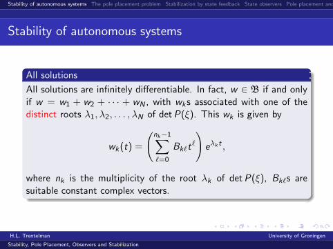
All solutions are infinitely differentiable. In fact, w ∈ B if and onlyif w = w1 + w2 + · · · + wN , with wks associated with one of thedistinct roots λ1, λ2, . . . , λN of det P(ξ). This wk is given by
wk(t) =
(
nk−1∑
`=0
Bk`t`
)
eλk t ,
where nk is the multiplicity of the root λk of det P(ξ), Bk`s aresuitable constant complex vectors.
H.L. Trentelman University of Groningen
Stability, Pole Placement, Observers and Stabilization
Stability of autonomous systems The pole placement problem Stabilization by state feedback State observers Pole placement and
Stability of autnomous systems
Stability definitions
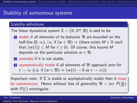
The linear dynamical system Σ = (R, Rq,B) is said to be
1 stable if all elements of its behavior B are bounded on thehalf-line [0,∞), i.e, if (w ∈ B) ⇒ (there exists M ∈ R suchthat ‖w(t)‖ ≤ M for t ≥ 0). Of course, this bound M
depends on the particular solution w ∈ B,
2 unstable if it is not stable,
3 asymptotically stable if all elements of B approach zero fort → ∞ (i.e, if (w ∈ B) ⇒ (w(t) → 0 as t → ∞)).
Important note: If Σ is stable or asymptotically stable then it mustbe autonomous. Hence without loss of generality B = ker P( d
dt)
with P(ξ) nonsingular.
H.L. Trentelman University of Groningen
Stability, Pole Placement, Observers and Stabilization

Stability of autonomous systems The pole placement problem Stabilization by state feedback State observers Pole placement and
Stability of autonomous systems
Definition of simple and semisimple roots
Let P(ξ) ∈ Rq×q[ξ] be nonsingular. Then
1 The roots of P(ξ) are defined to be those of the scalarpolynomial detP(ξ). Hence λ ∈ C is a root of P(ξ) if andonly if rank P(λ) < q,
2 The root λ is called simple if it is a root of det P(ξ) ofmultiplicity one,
3 semisimple if the rank deficiency of P(λ) equals themultiplicity of λ as a root of P(ξ) (equivalently, if thedimension of ker P(λ) is equal to the multiplicity of λ as aroot of det P(ξ)).
Clearly, for q = 1 roots are semisimple if and only if they are simple,but for q > 1 the situation is more complicated.
H.L. Trentelman University of Groningen
Stability, Pole Placement, Observers and Stabilization

Stability of autonomous systems The pole placement problem Stabilization by state feedback State observers Pole placement and
Stability of autonomous systems
Example
λ = 0 is a root of multiplicity 2 for both the polynomial matrices
(
ξ 00 ξ
)
and
(
ξ 10 ξ
)
. (1)
This root is semisimple in the first case, but not in the second.
H.L. Trentelman University of Groningen
Stability, Pole Placement, Observers and Stabilization

Stability of autonomous systems The pole placement problem Stabilization by state feedback State observers Pole placement and
Stability of autonomous systems
Theorem
Let P ∈ Rq×q[ξ] be nonsingular. The system represented by
P( d
dt)w = 0 is:
1 asymptotically stable if and only if all the roots of detP(ξ)have negative real part;
2 stable if and only if for each λ ∈ C that is a root of P(ξ),either (i) Re λ < 0, or (ii) Re λ = 0 and λ is a semisimpleroot of P(ξ).
3 unstable if P(ξ) has a root with positive real part and/or anonsemisimple root with zero real part.
H.L. Trentelman University of Groningen
Stability, Pole Placement, Observers and Stabilization

Stability of autonomous systems The pole placement problem Stabilization by state feedback State observers Pole placement and
Stability of autonomous systems
Examples
1 Scalar first-order system aw + ddt
w = 0. Associatedpolynomial P(ξ) = a + ξ. Root −a. Hence this system isasymptotically stable if a > 0, stable if a = 0, and unstable ifa < 0. Note: behavior B = {Ae−at | A ∈ R}.
2 Scalar second-order system aw + d2
dt2 w = 0. Associatedpolynomial P(ξ) = a + ξ2. Roots λ1,2 = ±
√−a for a < 0,
λ1,2 = ±i√
a for a > 0, and λ = 0 is a double, not semisimpleroot when a = 0. Thus we have (a < 0 ⇒ instability),(a > 0 ⇒ stability), and (a = 0 ⇒ instability). Indeed:B = {Ae
√−at + Be−
√−at | A,B ∈ R}, if a < 0,
B = {A cos√
at + B sin√
atA | A,B ∈ R}, if a > 0,B = {A + Bt | A,B ∈ R}, if a = 0.
H.L. Trentelman University of Groningen
Stability, Pole Placement, Observers and Stabilization

Stability of autonomous systems The pole placement problem Stabilization by state feedback State observers Pole placement and
Stability of autonomous systems
Special case: stability of state equations
Autonomous state system d
dtx = Ax , with A ∈ R
n×n.Polynomial matrix P(ξ) = Iξ − A. Roots: the eigenvalues of A.An eigenvalue λ of A is called semisimple if λ is a semisimple rootof det(Iξ − A), i.e:
the multiplicity of λ is equal to dim ker(λI − A).
Note: dim ker(λI−A) is always equal to the number of independenteigenvectors associated with the eigenvalue λ.
H.L. Trentelman University of Groningen
Stability, Pole Placement, Observers and Stabilization
Stability of autonomous systems The pole placement problem Stabilization by state feedback State observers Pole placement and
Stability of autonomous systems
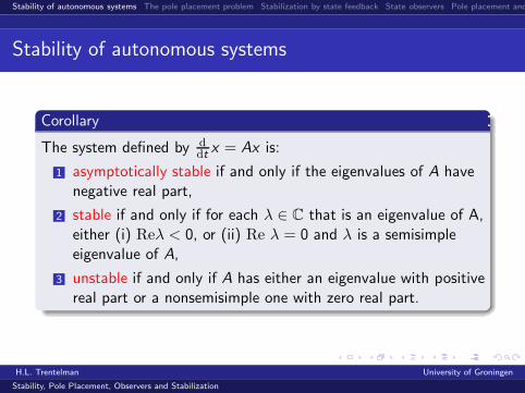
Corollary
The system defined by d
dtx = Ax is:
1 asymptotically stable if and only if the eigenvalues of A havenegative real part,
2 stable if and only if for each λ ∈ C that is an eigenvalue of A,either (i) Reλ < 0, or (ii) Re λ = 0 and λ is a semisimpleeigenvalue of A,
3 unstable if and only if A has either an eigenvalue with positivereal part or a nonsemisimple one with zero real part.
H.L. Trentelman University of Groningen
Stability, Pole Placement, Observers and Stabilization
Stability of autonomous systems The pole placement problem Stabilization by state feedback State observers Pole placement and
The pole placement problem
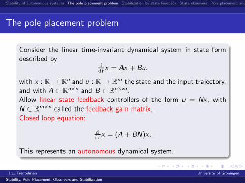
Consider the linear time-invariant dynamical system in state formdescribed by
d
dtx = Ax + Bu,
with x : R → Rn and u : R → R
m the state and the input trajectory,and with A ∈ R
n×n and B ∈ Rn×m.
Allow linear state feedback controllers of the form u = Nx , withN ∈ R
m×n called the feedback gain matrix.Closed loop equation:
d
dtx = (A + BN)x .
This represents an autonomous dynamical system.
H.L. Trentelman University of Groningen
Stability, Pole Placement, Observers and Stabilization

Stability of autonomous systems The pole placement problem Stabilization by state feedback State observers Pole placement and
Stability of Autonomous Systems
u = Nx
Plantddt
x = Ax + Bu
Feedback
processor
H.L. Trentelman University of Groningen
Stability, Pole Placement, Observers and Stabilization
Stability of autonomous systems The pole placement problem Stabilization by state feedback State observers Pole placement and
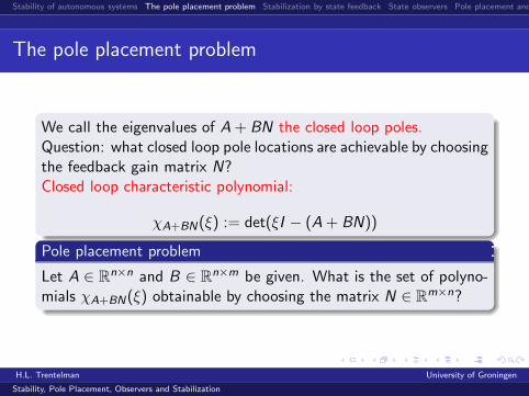
The pole placement problem
We call the eigenvalues of A + BN the closed loop poles.Question: what closed loop pole locations are achievable by choosingthe feedback gain matrix N?Closed loop characteristic polynomial:
χA+BN(ξ) := det(ξI − (A + BN))
Pole placement problem
Let A ∈ Rn×n and B ∈ R
n×m be given. What is the set of polyno-mials χA+BN(ξ) obtainable by choosing the matrix N ∈ R
m×n?
H.L. Trentelman University of Groningen
Stability, Pole Placement, Observers and Stabilization
Stability of autonomous systems The pole placement problem Stabilization by state feedback State observers Pole placement and
The pole placement problem
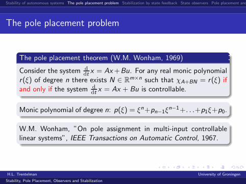
The pole placement theorem (W.M. Wonham, 1969)
Consider the system d
dtx = Ax +Bu. For any real monic polynomial
r(ξ) of degree n there exists N ∈ Rm×n such that χA+BN = r(ξ) if
and only if the system d
dtx = Ax + Bu is controllable.
Monic polynomial of degree n: p(ξ) = ξn+pn−1ξn−1+. . .+p1ξ+p0.
W.M. Wonham, ”On pole assignment in multi-input controllablelinear systems”, IEEE Transactions on Automatic Control, 1967.
H.L. Trentelman University of Groningen
Stability, Pole Placement, Observers and Stabilization
Stability of autonomous systems The pole placement problem Stabilization by state feedback State observers Pole placement and
Proof of the pole placement theorem
H.L. Trentelman University of Groningen
Stability, Pole Placement, Observers and Stabilization
Stability of autonomous systems The pole placement problem Stabilization by state feedback State observers Pole placement and
Proof of the pole placement theorem
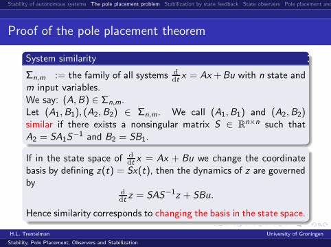
System similarity
Σn,m := the family of all systems d
dtx = Ax +Bu with n state and
m input variables.We say: (A,B) ∈ Σn,m.Let (A1,B1), (A2,B2) ∈ Σn,m. We call (A1,B1) and (A2,B2)similar if there exists a nonsingular matrix S ∈ R
n×n such thatA2 = SA1S
−1 and B2 = SB1.
If in the state space of d
dtx = Ax + Bu we change the coordinate
basis by defining z(t) = Sx(t), then the dynamics of z are governedby
d
dtz = SAS−1z + SBu.
Hence similarity corresponds to changing the basis in the state space.
H.L. Trentelman University of Groningen
Stability, Pole Placement, Observers and Stabilization
Stability of autonomous systems The pole placement problem Stabilization by state feedback State observers Pole placement and
Proof of the pole placement theorem
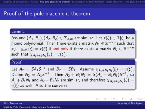
Lemma
Assume (A1,B1), (A2,B2) ∈ Σn,m are similar. Let r(ξ) ∈ R[ξ] be amonic polynomial. Then there exists a matrix N1 ∈ Rm×n such thatχA1+B1N1
(ξ) = r(ξ) if and only if there exists a matrix N2 ∈ Rm×n
such that χA2+B2N2(ξ) = r(ξ).
Proof
Let A2 = SA1S−1 and B2 = SB1. Assume χA1+B1N1
(ξ) = r(ξ).Define N2 = N1S
−1. Then A2 + B2N2 = S(A1 + B1N1)S−1, so
A1 +B1N1 and A2 +B2N2 are similar, and therefore χA2+B2N2(ξ) =
r(ξ) as well. Also the converse.
H.L. Trentelman University of Groningen
Stability, Pole Placement, Observers and Stabilization
Stability of autonomous systems The pole placement problem Stabilization by state feedback State observers Pole placement and
Proof of the pole placement theorem
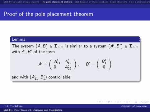
Lemma
The system (A,B) ∈ Σn,m is similar to a system (A′,B ′) ∈ Σn,m
with A′,B ′ of the form
A′ =
(
A′11 A′
12
0 A′22
)
, B ′ =
(
B ′1
0
)
and with (A′11,B
′1) controllable.
H.L. Trentelman University of Groningen
Stability, Pole Placement, Observers and Stabilization

Stability of autonomous systems The pole placement problem Stabilization by state feedback State observers Pole placement and
Proof of the pole placement theorem
Proof
Two cases:
1 if (A,B) is controllable then A′11 = A′ = A and B ′
1 = B ′ = B ,and A′
12, A′22 and the 0-matrices are ’void’.
2 If (A,B) is not controllable, thenR := im(B AB A2B . . . An−1B) 6= R
n, so is a proper subspaceof R
n. Choose a basis of Rn adapted to R. The matrices with
respect to this new basis are of the form (A′,B ′) becauseAR ⊂ R and im B ⊂ R.
H.L. Trentelman University of Groningen
Stability, Pole Placement, Observers and Stabilization
Stability of autonomous systems The pole placement problem Stabilization by state feedback State observers Pole placement and
Proof of the pole placement theorem
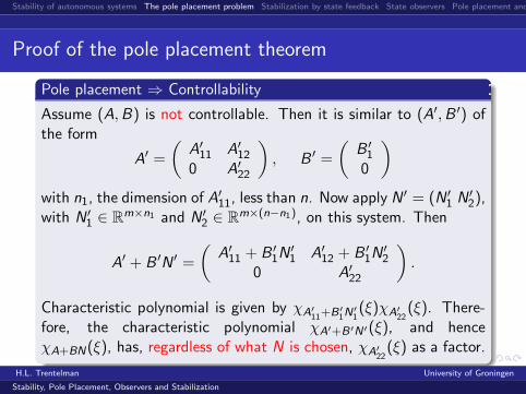
Pole placement ⇒ Controllability
Assume (A,B) is not controllable. Then it is similar to (A′,B ′) ofthe form
A′ =
(
A′11 A′
12
0 A′22
)
, B ′ =
(
B ′1
0
)
with n1, the dimension of A′11, less than n. Now apply N ′ = (N ′
1 N ′2),
with N ′1 ∈ R
m×n1 and N ′2 ∈ R
m×(n−n1), on this system. Then
A′ + B ′N ′ =
(
A′11 + B ′
1N′1 A′
12 + B ′1N
′2
0 A′22
)
.
Characteristic polynomial is given by χA′
11+B′
1N′
1(ξ)χA′
22(ξ). There-
fore, the characteristic polynomial χA′+B′N′(ξ), and henceχA+BN(ξ), has, regardless of what N is chosen, χA′
22(ξ) as a factor.
H.L. Trentelman University of Groningen
Stability, Pole Placement, Observers and Stabilization
Stability of autonomous systems The pole placement problem Stabilization by state feedback State observers Pole placement and
Proof of the pole placement theorem
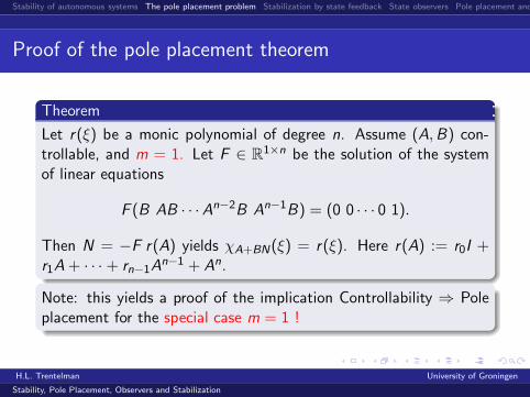
Theorem
Let r(ξ) be a monic polynomial of degree n. Assume (A,B) con-trollable, and m = 1. Let F ∈ R
1×n be the solution of the systemof linear equations
F (B AB · · ·An−2B An−1B) = (0 0 · · · 0 1).
Then N = −F r(A) yields χA+BN(ξ) = r(ξ). Here r(A) := r0I +r1A + · · · + rn−1A
n−1 + An.
Note: this yields a proof of the implication Controllability ⇒ Poleplacement for the special case m = 1 !
H.L. Trentelman University of Groningen
Stability, Pole Placement, Observers and Stabilization
Stability of autonomous systems The pole placement problem Stabilization by state feedback State observers Pole placement and
Proof of the pole placement theorem
Notation
Σcontn,m ⊂ Σn,m are all controllable systems with state space R
n andinput space R
m.
Heymann’s lemma (1968)
Let (A,B) ∈ Σcontn,m . Assume K ∈ R
m×1 such that BK 6= 0.Then there exists a N ′ ∈ R
m×n such that (A + BN ′,BK ) ∈ Σcont1,n .
M. Heymann, ”Comments to: Pole assignment in multi-input con-trollable linear systems”, IEEE Transactions on Automatic Control,1968.
H.L. Trentelman University of Groningen
Stability, Pole Placement, Observers and Stabilization
Stability of autonomous systems The pole placement problem Stabilization by state feedback State observers Pole placement and
Proof of the pole placement theorem
H.L. Trentelman University of Groningen
Stability, Pole Placement, Observers and Stabilization

Stability of autonomous systems The pole placement problem Stabilization by state feedback State observers Pole placement and
Proof of the pole placement theorem
Controllability ⇒ Pole placement, m > 1: coup de grace
Choose K ∈ Rm×1 such that BK 6= 0, by controllability, B 6= 0,
hence such a K exists.Choose N ′ ∈ R
m×1 such that (A + BN ′,BK ) controllable.We are now back in the case m = 1.Choose N ′′ ∈ R
1×n such that A + BN ′ + BKN ′′ has the desiredcharacteristic polynomial r(ξ).Finally, take N = N ′ + KN ′′.Then A + BN = A + BN ′ + BKN ′′ so χA+BN(ξ) = r(ξ).
H.L. Trentelman University of Groningen
Stability, Pole Placement, Observers and Stabilization

Stability of autonomous systems The pole placement problem Stabilization by state feedback State observers Pole placement and
The pole placement problem
Algorithm
Data: A ∈ Rn×n, B ∈ R
n×m, with (A,B) controllable; r(ξ) ∈ R[ξ]with r(ξ) monic and of degree n.Required: N ∈ R
m×n such that χA+BN(ξ) = r(ξ).Algorithm:
1 Find K ∈ Rm×1 and N ′ ∈ R
m×n such that (A + BN ′,BK ) iscontrollable.
2 Put A′ = A + BN ′, B ′ = BK , and compute F from
F [B ′,A′B ′, . . . , (A′)n−1B ′] = [0 0 . . . 0 1].
3 Compute N ′′ = −F r(A′).
4 Compute N = N ′ + KN ′′.
Result: N is the desired feedback matrix.
H.L. Trentelman University of Groningen
Stability, Pole Placement, Observers and Stabilization
Stability of autonomous systems The pole placement problem Stabilization by state feedback State observers Pole placement and
Stabilization
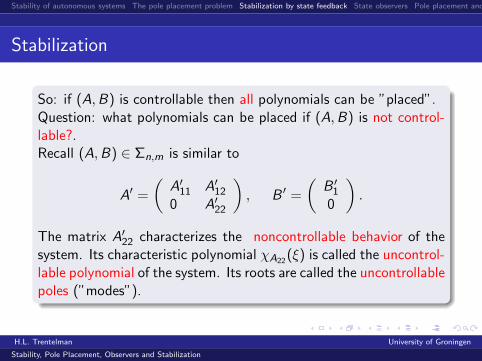
So: if (A,B) is controllable then all polynomials can be ”placed”.Question: what polynomials can be placed if (A,B) is not control-lable?.Recall (A,B) ∈ Σn,m is similar to
A′ =
(
A′11 A′
12
0 A′22
)
, B ′ =
(
B ′1
0
)
.
The matrix A′22 characterizes the noncontrollable behavior of the
system. Its characteristic polynomial χA22(ξ) is called the uncontrol-
lable polynomial of the system. Its roots are called the uncontrollablepoles (”modes”).
H.L. Trentelman University of Groningen
Stability, Pole Placement, Observers and Stabilization
Stability of autonomous systems The pole placement problem Stabilization by state feedback State observers Pole placement and
Stabilization
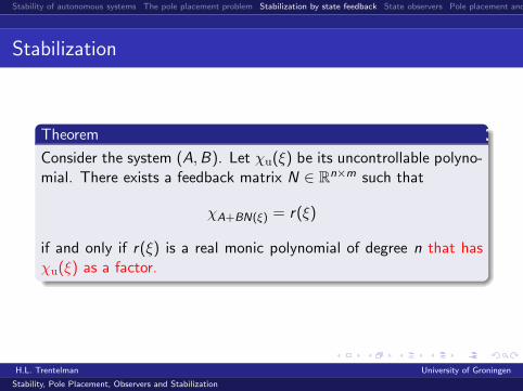
Theorem
Consider the system (A,B). Let χu(ξ) be its uncontrollable polyno-mial. There exists a feedback matrix N ∈ R
n×m such that
χA+BN(ξ) = r(ξ)
if and only if r(ξ) is a real monic polynomial of degree n that hasχu(ξ) as a factor.
H.L. Trentelman University of Groningen
Stability, Pole Placement, Observers and Stabilization
Stability of autonomous systems The pole placement problem Stabilization by state feedback State observers Pole placement and
Stabilization
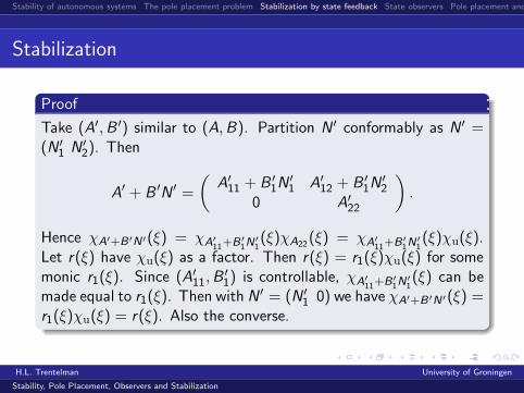
Proof
Take (A′,B ′) similar to (A,B). Partition N ′ conformably as N ′ =(N ′
1 N ′2). Then
A′ + B ′N ′ =
(
A′11 + B ′
1N′1 A′
12 + B ′1N
′2
0 A′22
)
.
Hence χA′+B′N′(ξ) = χA′
11+B′
1N′
1(ξ)χA22
(ξ) = χA′
11+B′
1N′
1(ξ)χu(ξ).
Let r(ξ) have χu(ξ) as a factor. Then r(ξ) = r1(ξ)χu(ξ) for somemonic r1(ξ). Since (A′
11,B′1) is controllable, χA′
11+B′
1N′
1(ξ) can be
made equal to r1(ξ). Then with N ′ = (N ′1 0) we have χA′+B′N′(ξ) =
r1(ξ)χu(ξ) = r(ξ). Also the converse.
H.L. Trentelman University of Groningen
Stability, Pole Placement, Observers and Stabilization
Stability of autonomous systems The pole placement problem Stabilization by state feedback State observers Pole placement and
Stabilization
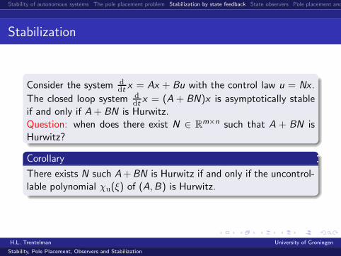
Consider the system d
dtx = Ax + Bu with the control law u = Nx .
The closed loop system d
dtx = (A + BN)x is asymptotically stable
if and only if A + BN is Hurwitz.Question: when does there exist N ∈ R
m×n such that A + BN isHurwitz?
Corollary
There exists N such A + BN is Hurwitz if and only if the uncontrol-lable polynomial χu(ξ) of (A,B) is Hurwitz.
H.L. Trentelman University of Groningen
Stability, Pole Placement, Observers and Stabilization
Stability of autonomous systems The pole placement problem Stabilization by state feedback State observers Pole placement and
Stabilization
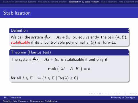
Definition
We call the system d
dtx = Ax +Bu, or, equivalently, the pair (A,B),
stabilizable if its uncontrollable polynomial χu(ξ) is Hurwitz.
Theorem (Hautus test)
The system d
dtx = Ax + Bu is stabilizable if and only if
rank(
λI − A B)
= n
for all λ ∈ C+ := {λ ∈ C | Re(λ) ≥ 0}.
H.L. Trentelman University of Groningen
Stability, Pole Placement, Observers and Stabilization

Stability of autonomous systems The pole placement problem Stabilization by state feedback State observers Pole placement and
Stabilization
H.L. Trentelman University of Groningen
Stability, Pole Placement, Observers and Stabilization
Stability of autonomous systems The pole placement problem Stabilization by state feedback State observers Pole placement and
State observers
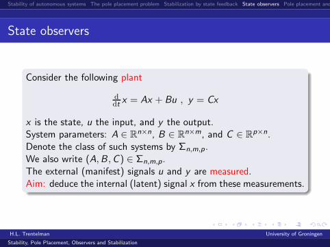
Consider the following plant
d
dtx = Ax + Bu , y = Cx
x is the state, u the input, and y the output.System parameters: A ∈ R
n×n, B ∈ Rn×m, and C ∈ R
p×n.Denote the class of such systems by Σn,m,p.We also write (A,B ,C ) ∈ Σn,m,p.The external (manifest) signals u and y are measured.Aim: deduce the internal (latent) signal x from these measurements.
H.L. Trentelman University of Groningen
Stability, Pole Placement, Observers and Stabilization

Stability of autonomous systems The pole placement problem Stabilization by state feedback State observers Pole placement and
State observers
D. Luenberger, 1963
H.L. Trentelman University of Groningen
Stability, Pole Placement, Observers and Stabilization

Stability of autonomous systems The pole placement problem Stabilization by state feedback State observers Pole placement and
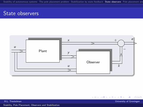
State observers
An algorithm that estimates x from u and y is called a state observer.Denote the estimate of x by x , and define the estimation error as
e := x − x .
A state observer is a dynamical system with u and y as input, x asoutput, and that makes e = x − x small in some sense.Here we focus on the asymptotic behavior of e(t) for t → ∞.
H.L. Trentelman University of Groningen
Stability, Pole Placement, Observers and Stabilization
Stability of autonomous systems The pole placement problem Stabilization by state feedback State observers Pole placement and
State observers
Plant
Observer
y
x
u
+
−
e
u
x
H.L. Trentelman University of Groningen
Stability, Pole Placement, Observers and Stabilization
Stability of autonomous systems The pole placement problem Stabilization by state feedback State observers Pole placement and
State observers
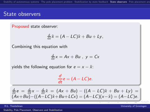
Proposed state observer:
d
dtx = (A − LC )x + Bu + Ly ,
Combining this equation with
d
dtx = Ax + Bu , y = Cx
yields the following equation for e = x − x :
d
dte = (A − LC )e.
d
dte = d
dtx − d
dtx = (Ax + Bu) − ((A − LC )x + Bu + Ly) =
(Ax+Bu)−((A−LC )x+Bu+LCx) = (A−LC )(x−x) = (A−LC )e.
H.L. Trentelman University of Groningen
Stability, Pole Placement, Observers and Stabilization
Stability of autonomous systems The pole placement problem Stabilization by state feedback State observers Pole placement and
State observers
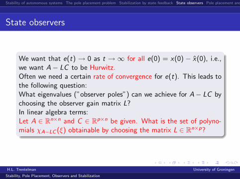
We want that e(t) → 0 as t → ∞ for all e(0) = x(0) − x(0), i.e.,we want A − LC to be Hurwitz.Often we need a certain rate of convergence for e(t). This leads tothe following question:What eigenvalues (”observer poles”) can we achieve for A − LC bychoosing the observer gain matrix L?In linear algebra terms:Let A ∈ R
n×n and C ∈ Rp×n be given. What is the set of polyno-
mials χA−LC (ξ) obtainable by choosing the matrix L ∈ Rn×p?
H.L. Trentelman University of Groningen
Stability, Pole Placement, Observers and Stabilization

Stability of autonomous systems The pole placement problem Stabilization by state feedback State observers Pole placement and
State observers
Theorem
Consider the system d
dtx = Ax + Bu , y = Cx . There exists for
every real monic polynomial r(ξ) of degree n a matrix L such thatχA−LC (ξ) equals r(ξ) if and only if the system is observable.
Proof
(A,C ) observable pair if and only if (AT ,CT ) controllable pair.Note: for any real square matrix M, χM(ξ) = χMT (ξ). Assume(A,C ) observable. By the pole placement theorem, there exists forall r(ξ) a matrix N ∈ R
p×n such that χAT +CTN(ξ) = r(ξ). ThusχA−LC (ξ) = r(ξ) with L = −NT .Conversely: Assume there exists for all r(ξ) a matrix L ∈ R
n×p suchthat χA−LC (ξ) = r(ξ). Then χAT +CT (−L)T (ξ) = r(ξ) so (AT ,CT )controllable, whence (A,C ) observable.
H.L. Trentelman University of Groningen
Stability, Pole Placement, Observers and Stabilization

Stability of autonomous systems The pole placement problem Stabilization by state feedback State observers Pole placement and
State observers
What if (A,C ) is not observable?The dynamical systems (A1,B1,C1) ∈ Σn,m,p and (A2,B2,C2) ∈Σn,m,p are called similar if there exist a nonsingular S such thatA1 = SA2S
−1, B1 = SB2, C1 = C2S−1.
Theorem
The system (A,B ,C ) ∈ Σn,m,p is similar to a system of the form(A′,B ′,C ′) in which A′ and C ′ have the following structure:
A′ =
(
A11 0A12 A22
)
, C ′ = (C1 0),
with (A11,C1) observable.All such decompositions lead to matrices A22 that have the samecharacteristic polynomial.
H.L. Trentelman University of Groningen
Stability, Pole Placement, Observers and Stabilization
Stability of autonomous systems The pole placement problem Stabilization by state feedback State observers Pole placement and
State observers
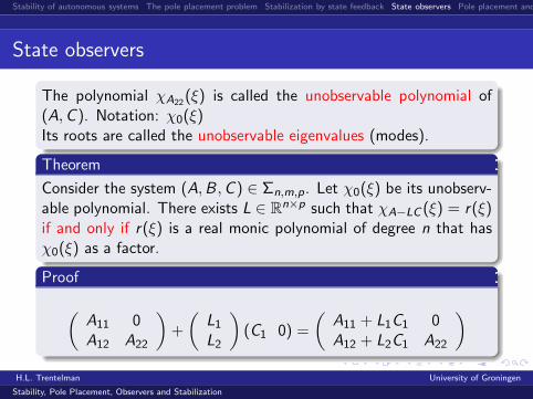
The polynomial χA22(ξ) is called the unobservable polynomial of
(A,C ). Notation: χ0(ξ)Its roots are called the unobservable eigenvalues (modes).
Theorem
Consider the system (A,B ,C ) ∈ Σn,m,p. Let χ0(ξ) be its unobserv-able polynomial. There exists L ∈ R
n×p such that χA−LC (ξ) = r(ξ)if and only if r(ξ) is a real monic polynomial of degree n that hasχ0(ξ) as a factor.
Proof
(
A11 0A12 A22
)
+
(
L1
L2
)
(C1 0) =
(
A11 + L1C1 0A12 + L2C1 A22
)
H.L. Trentelman University of Groningen
Stability, Pole Placement, Observers and Stabilization

Stability of autonomous systems The pole placement problem Stabilization by state feedback State observers Pole placement and
State observers
Corollary
There exists an observer d
dtx = (A− LC )x + Bu + Ly such that for
all initial states x(0) and x(0)
limt→∞
x(t) − x(t) = 0,
i.e. such that A − LC is Hurwitz, if and only if the unobservablepolynomial χ0(ξ) of (A,C ) is Hurwitz.
Definition
The system (A,B ,C ) ∈ Σn,m,p is called detectable if the the unob-servable polynomial χ0(ξ) of (A,C ) is Hurwitz.
H.L. Trentelman University of Groningen
Stability, Pole Placement, Observers and Stabilization
Stability of autonomous systems The pole placement problem Stabilization by state feedback State observers Pole placement and
State observers
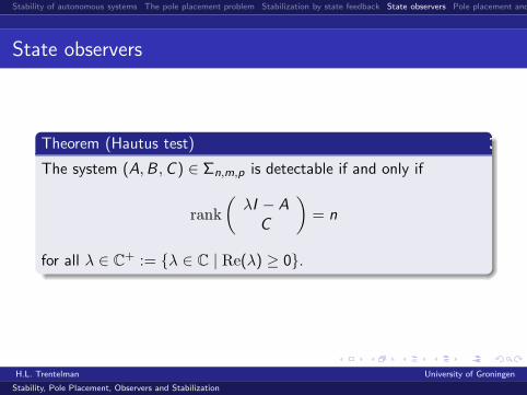
Theorem (Hautus test)
The system (A,B ,C ) ∈ Σn,m,p is detectable if and only if
rank
(
λI − A
C
)
= n
for all λ ∈ C+ := {λ ∈ C | Re(λ) ≥ 0}.
H.L. Trentelman University of Groningen
Stability, Pole Placement, Observers and Stabilization

Stability of autonomous systems The pole placement problem Stabilization by state feedback State observers Pole placement and
Dynamic output feedback
Plant:d
dtx = Ax + Bu , y = Cx .
Linear time-invariant feedback controller:
d
dtz = Kz + Ly , u = Mz + Ny ,
with z : R → Rd the state of the controller, K ∈ R
d×d , L ∈ Rd×p,
M ∈ Rm×d , and N ∈ R
m×p the parameter matrices specifying thecontroller.State dimension d ∈ N is called the order of the controller. Is adesign parameter: typically, we want d to be small.
H.L. Trentelman University of Groningen
Stability, Pole Placement, Observers and Stabilization
Stability of autonomous systems The pole placement problem Stabilization by state feedback State observers Pole placement and
Dynamic output feedback
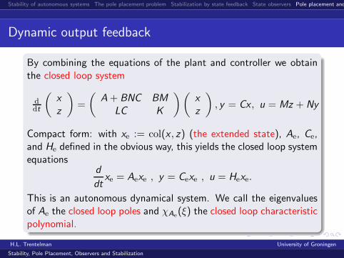
By combining the equations of the plant and controller we obtainthe closed loop system
d
dt
(
x
z
)
=
(
A + BNC BM
LC K
)(
x
z
)
, y = Cx , u = Mz + Ny
Compact form: with xe := col(x , z) (the extended state), Ae, Ce,and He defined in the obvious way, this yields the closed loop systemequations
d
dtxe = Aexe , y = Cexe , u = Hexe.
This is an autonomous dynamical system. We call the eigenvaluesof Ae the closed loop poles and χAe
(ξ) the closed loop characteristicpolynomial.
H.L. Trentelman University of Groningen
Stability, Pole Placement, Observers and Stabilization
Stability of autonomous systems The pole placement problem Stabilization by state feedback State observers Pole placement and
Dynamic output feedback
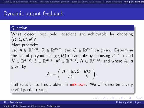
Question
What closed loop pole locations are achievable by choosing(K ,L,M,N)?More precisely:Let A ∈ R
n×n, B ∈ Rn×m, and C ∈ R
p×n be given. Determinethe set of polynomials χAe
(ξ) obtainable by choosing d ∈ N andK ∈ R
d×d , L ∈ Rd×p, M ∈ R
m×d , N ∈ Rm×p, and where Ae is
given by
Ae =
(
A + BNC BM
LC K
)
.
Full solution to this problem is unknown. We will describe a veryuseful partial result.
H.L. Trentelman University of Groningen
Stability, Pole Placement, Observers and Stabilization
Stability of autonomous systems The pole placement problem Stabilization by state feedback State observers Pole placement and
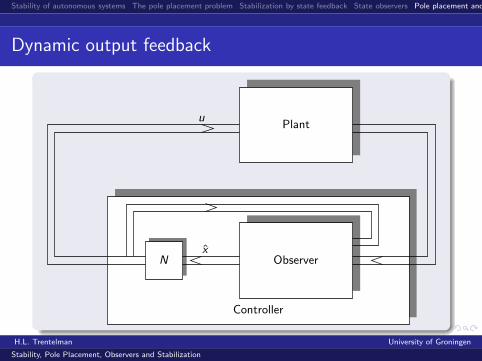
Dynamic output feedback
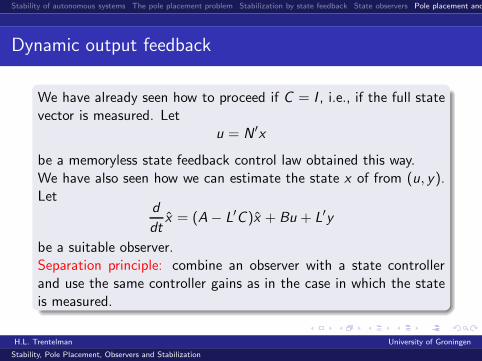
We have already seen how to proceed if C = I , i.e., if the full statevector is measured. Let
u = N ′x
be a memoryless state feedback control law obtained this way.We have also seen how we can estimate the state x of from (u, y).Let
d
dtx = (A − L′C )x + Bu + L′y
be a suitable observer.Separation principle: combine an observer with a state controllerand use the same controller gains as in the case in which the stateis measured.
H.L. Trentelman University of Groningen
Stability, Pole Placement, Observers and Stabilization
Stability of autonomous systems The pole placement problem Stabilization by state feedback State observers Pole placement and
Dynamic output feedback
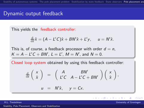
This yields the feedback controller:
d
dtx = (A − L′C )x + BN ′x + L′y , u = N ′x .
This is, of course, a feedback processor with order d = n,K = A − L′C + BN ′, L = L′, M = N ′, and N = 0.
Closed loop system obtained by using this feedback controller:
d
dt
(
x
x
)
=
(
A BN ′
L′C A − L′C + BN ′
)(
x
x
)
,
u = N ′x , y = Cx .
H.L. Trentelman University of Groningen
Stability, Pole Placement, Observers and Stabilization
Stability of autonomous systems The pole placement problem Stabilization by state feedback State observers Pole placement and
Dynamic output feedback
N
Plant
Controller
u
xObserver
H.L. Trentelman University of Groningen
Stability, Pole Placement, Observers and Stabilization
Stability of autonomous systems The pole placement problem Stabilization by state feedback State observers Pole placement and
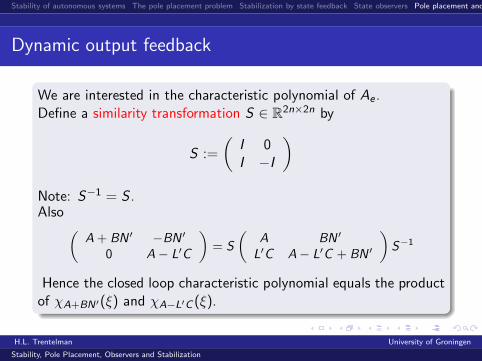
Dynamic output feedback
We are interested in the characteristic polynomial of Ae .Define a similarity transformation S ∈ R
2n×2n by
S :=
(
I 0I −I
)
Note: S−1 = S .Also
(
A + BN ′ −BN ′
0 A − L′C
)
= S
(
A BN ′
L′C A − L′C + BN ′
)
S−1
Hence the closed loop characteristic polynomial equals the productof χA+BN′(ξ) and χA−L′C (ξ).
H.L. Trentelman University of Groningen
Stability, Pole Placement, Observers and Stabilization

Stability of autonomous systems The pole placement problem Stabilization by state feedback State observers Pole placement and
Dynamic output feedback
Theorem (Pole placement by dynamic output feedback)
Consider the system (A,B ,C ) and assume that (A,B) is control-lable and that (A,C ) is observable.Then for every real monic polynomial r(ξ) of degree 2n, factoriz-able into two real polynomials of degree n, there exists a feedbackcontroller (K ,L,M,N) of order n such that the closed loop systemmatrix Ae has characteristic polynomial r(ξ).
Proof
Take d = n, K = A − L′C + BN ′, L = L′, M = N ′, andN = 0. Choose N ′ such that χA+BN′(ξ) = r1(ξ) and L′ such thatχA−L′C (ξ) = r2(ξ), where r1(ξ) and r2(ξ) are real factors of r(ξ)such that r(ξ) = r1(ξ)r2(ξ).
H.L. Trentelman University of Groningen
Stability, Pole Placement, Observers and Stabilization

Stability of autonomous systems The pole placement problem Stabilization by state feedback State observers Pole placement and
Dynamic output feedback
Theorem (Stabilization by dynamic output feedback)
Consider the system (A,B ,C ) and let χu(ξ) be its uncontrollablepolynomial, χ0(ξ) its unobservable polynomial. Then
1 For any real monic polynomials r1(ξ) and r2(ξ) of degree n
such that r1(ξ) has χu(ξ) as a factor and r2(ξ) has χ0(ξ) as afactor, there exists a feedback controller (K ,L,M,N) of ordern such that the closed loop system matrix Ae hascharacteristic polynomial r(ξ) = r1(ξ)r2(ξ).
2 There exists a feedback controller (K ,L,M,N) as such thatthe closed loop system is asymptotically stable if and only ifboth χu(ξ) and χ0(ξ) are Hurwitz, i.e., if and only if (A,B) isstabilizable and (A,C ) is detectable.
H.L. Trentelman University of Groningen
Stability, Pole Placement, Observers and Stabilization