FEEDBACK SYSTEM DESIGN: THE POLE PLACEMENT PROBLEM

by

ASHOK IYER, B.E., M.S.E.E.

A DISSERTATION

IN

ELECTRICAL ENGINEERING

Submitted to the Graduate Faculty of Texas Tech University in

Partial Fulfillment of the Requirements for

the Degree of

DOCTOR OF PHILOSOPHY

Approved

December, 1982

7 :-

ACKNOWLEDGEMENTS

I would like to express my sincere thanks to Horn Professor

Richard E. Saeks for his expert guidance of this dissertation.

Professors John Murray, Louis Hunt, William Portnoy and John Walkup

for serving on my committee. Dr. Erol Emre for many interesting

conservations and helpful comments and Mr. Chin-Long Wey for helping

me with the multivariate-example. It is a pleasure acknowledging

their help.

Finally a special thanks to my parents, brother, sisters and

friends for their encouragement and support during my entire edu­

cation.

n

TABLE OF CONTENTS

ACKNOWLEDGEMENTS i i

LIST OF FIGURES v

CHAPTER 1 INTRODUCTION 1

1.1 Fractional Representation Theory: Historial Background ,. 2

1.2 Fractional Representation Theory: Mathematical Preliminaries 3

1.3 Stablization 4

Theorem 1.1: Stabilization Theorem . . . . 8

CHAPTER 2 THE SINGLE VARIATE POLE PLACEMENT PROBLEM. . . . 9

2.1 The Single Variate Pole Placement Problem . 9

Theorem 2.1 11

Proof: Sufficiency 11

Necessity 14

Corollary 2.1 15

Proof 15

2.2 Proper and Strictly Proper Plants 17

Case i 18

Case ii 18

Case iii 18

Case iv 19

2.3 Improper Plants 20

Case i 20

Case ii 20

m

Theorem 2.2: Pole Placement Theorem. . . . 21

2.4 Parameterization of Solution Space 21

Corollary 2.2 27

CHAPTER 3 THE STABLE MULTIVARIATE POLE PLACEMENT PROBLEM . 28

3.1 Multivariate Fractional Representation

Theory 28

3.2 The Stable Pole Placement Problem 30

Theorem 3.1 : Stable Pole Placement

Theorem 34

Proof 34

CHAPTER 4 EXAMPLES 39

Example 4.1: Unstable Proper Plant 39

Example 4.2: Stable Proper Plant 42

Example 4.3: Stable Multivariate Plant 46

CHAPTER 5 CONCLUDING REMARKS 49

REFERENCES 51

TV

LIST OF FIEUPvES

Figure 1 .1 : Basic Feedliack Systen , , . , , , , , , . . ^

Figure 4 . 1 : Unstable Plant Before Pole Placement and Stab iHzat lo i , . . - ^ . . . . . . . . . . 5$

Figure 4.2: Feedback System for Example 4.1 t+at Places 1:+« ? i ) ' l ^

of the System at Zeros of q(.s.) = s2+2+l . . . . . . . . . . . . . . . ^

Figure 4.3: Plant Before Stablllzat-icn ard Pole Plac«n»nt . . . . . . . . . . . 41:3

Figure 4 .4 : Feedlack System for Example 4.1 t t e t Places ^'1«5 ittt Zeros of q(s) = (s+ZJts+S) 415

CHAPTER 1

INTRODUCTION

Ever since Meikle invented the first control system in 1750

which automatically steered windmills to face the direction of the

wind, control systems have always been a great boon to man. Meikle's

invention was followed by a spate of control system inventions

during the Industrial Revolution. At about the same time Fourier

and Laplace proposed their transform techniques which are exten­

sively used in electrical engineering, especially in control

theory.

Control theory began to evolve with the advent of Cauchy's

mathematical work and the publication of two classical papers by

Nyquist titled 'Regeneration Theory' in 1932 and Hazen's paper

'Theory of Servomechanism' in 1934. The biggest boost was re­

ceived during World War II when the need for automatic control

systems was acute.

The advent of the space programs in the sixties brought about

the emergence of modern control theory. As a result of this rapid

progress, the systematic design of control systems is an everyday

affair now. Control theory is still a \iery active area of research,

and has spread in various directions. One of the latest is the for­

mulation of an algebraic fractional representation for the feedback

system design problem. This dissertation hopes to make a modest

contribution to the solution of the classical Pole Placement Prob­

lem [5],[6],[12],[25],[42],[53] in the algebraic fractional repre­

sentation setting. 1

1.1 Fractional Represenation Theory: Historical Background

In 1976 Youla, Bongiorno and Jabr published two classical

papers [57], [58] in which a complete parameterization of a set of

stablizing compensators for a multivariate feedback system was ob­

tained. In the ensuing years this work, often referred to as the

YBJ theory, has lead to the development of an entirely new approach

to feedback system design. This stabilization theory has been ap­

plied to some of the classical control problems such as:

1) Tracking and disturbance rejection [43],[45],[46]

2) Robust design algorithms [9],[45],[46]

3) Design with proper stable compensators [11],[45],[46]

4) Transfer function design [45],[46]

5) Simulataneous Design [9],[46]

6) Pole Placement [45],[46]

The pole placement problem has been extensively studied by the

author and is the problem solved in this disseration.

The key to the YBJ theory is a three step design philosophy:

1) Stabilization

2) Achievement of design constraints

3) Optimization of system performance

First and foremost, a feedback system must be stable and hence

the first step in the design process is the parameterization of all

stabilizing compensators for the given plant. Although it might

suffice to design a stable system, in practice stabilization is

only the first step of the design process. We must characterize

all compensators if we are to choose among the stabilizing

compensators to find one which also achieves the design constraints.

Once the stabilizing compensators have been characterized, we must

choose a subset of compensators which achieve a prescribed set of

design contraints, in this case the subset of compensators which

places poles for the given plant.

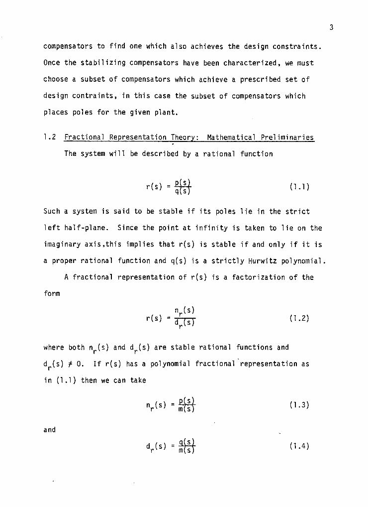
1.2 Fractional Representation Theory: Mathematical Preliminaries

The system will be described by a rational function

r-{s)=£|ff (1.1)

Such a system is said to be stable i f i t s poles l i e in the s t r i c t

l e f t half-plane. Since the point at i n f i n i t y is taken to l i e on the

imaginary axis, th is implies that r(s) is stable i f and only i f i t is

a proper rational function and q(s) is a s t r i c t l y Hurwitz polynomial.

A fract ional representation of r(s) is a factor izat ion of the

form

nJs ) r ( s ) = ^ (1.2)

where both n (s) and d (s) are stable rational functions and

d (s) t 0. If r(s) has a polynomial fractional representation as

in (1.1) then we can take

and

"r( = )=Stit f - i

V ^ ) = ^ (i-^)

where m(s) is any Hurwitz polynomial such that the order of m(s)

equals the order of r(s), verifying the existence of the required

fractional representation [20],

The fractional representation (1.2) is said to be 'coprime' if

there exists stable rational functions u (s) and v (s) such that

u^(s)n^(s) + v^(s)d^(s) - 1 (1.5)

In the case of polynomials (1.5) is the equivalent to the requ i re ­

ment tha t n (s) and d (s) have no common zeros [ 2 ] . In the ra t i ona l

f r ac t i ona l representa t ion, equation (1.5) implies tha t n (s) and

d (s) have no common r i g h t hal f -p lane zeros and conversely [ 7 ] , [ 2 0 ] .

One can j u s t i f y t h i s representat ion even though i t deviates from the

c lass ica l contro l theory, since only r i g h t ha l f -p lane zeros cause

i n s t a b i l i t i e s and t h i s theory forb ids the cance l la t ion of r i g h t

ha l f -p lane poles and zeros.

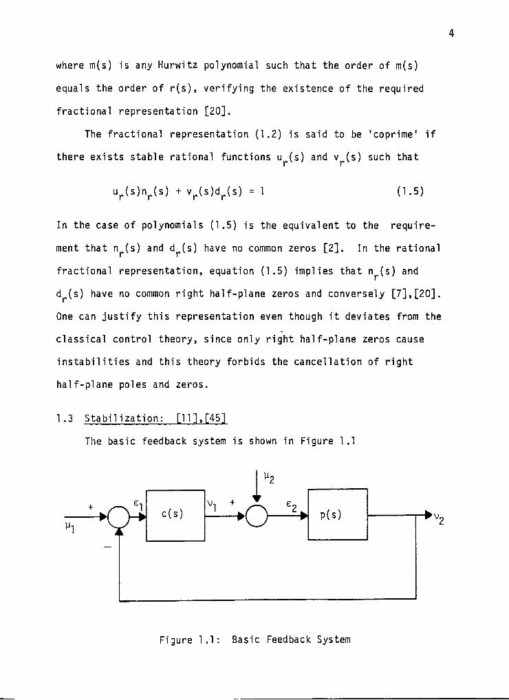
1 .3 S t a b i l i z a t i o n : [ 11 ] , [ 45 ]

The basic feedback system is shown in Figure 1.1

Figure 1 . 1 : Basic Feedback System

Using the usual algebraic manipulation [11], the following

system gains are obtained:

^^(s)

£2(5)

:;i

L K.uM^ h (s)

•2 2 ^2^1 • ' ^^l^c

yi(s)

y9(s)

1

(1.6)

where

h ,, (s), h (s) ^ih ^-[^2

L h (s) ^2h

h (s) £2 12

1+P(s)c(s)

c(s) 1+P(s)c(s)

-P(s)^ ^ 1+P(s)c(s)

1 1+P(s)c(s)

(1.7)

and

VT(S)

^2(5)

'W 'W

\> 1, (2) h (s) ^2h ^2^2

Uiis)

yo(s)

(1.8)

where

\> 1, (2) h (s)

K 1, (s) h (s) ^2h ^2^2

h- ,, (s) h (s) - 1 2 1 2 '2

L l-h^ (s) -h (s)

J

.cisl l+p(s)c(s)

p(s)c(s) l+p(s)c(s)

-P(s)c(s) 1+P(s)c(s)

P(s) , l+p(s)c(s)

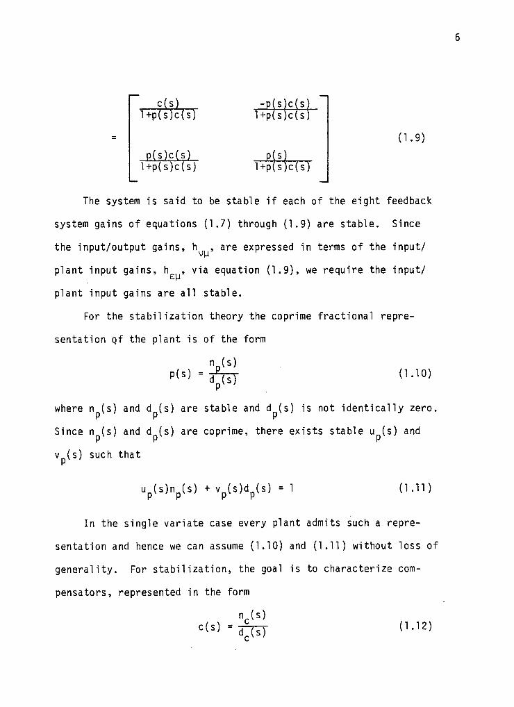
(1.9)

The system is said to be stable if each of the eight feedback

system gains of equations (1.7) through (1.9) are stable. Since

the input/output gains, h , are expressed in terms of the input/

plant input gains, h , via equation (1.9), we require the input/

plant input gains are all stable.

For the stabilization theory the coprime fractional repre­

sentation pf the plant is of the form

nn(s) P(s) dp(s) (1.10)

where n (s) and d (s) are stable and d (s) is not identically zero, p \ / p P

Since n (s) and d (s) are coprime, there exists stable u„(s) and

V (s) such that

Up(s)np(s) + Vp(s)dp(s) = 1 (1.11)

In the single variate case every plant admits such a repre­

sentation and hence we can assume (1.10) and (1.11) without loss of

generality. For stabilization, the goal is to characterize com­

pensators, represented in the form

n^(s) (1.12)

where n (s) and d (s) are stable and d (s) is not ident ical ly zero,

In order to prevent pole-zero cancellations between p(s) and c(s)

in the r ight half plane, a stronger condition namely

n (s)n (s)

'^'^'^'^ - dp(s)d^(s) (1.13)

be a coprime fractional representation is required.

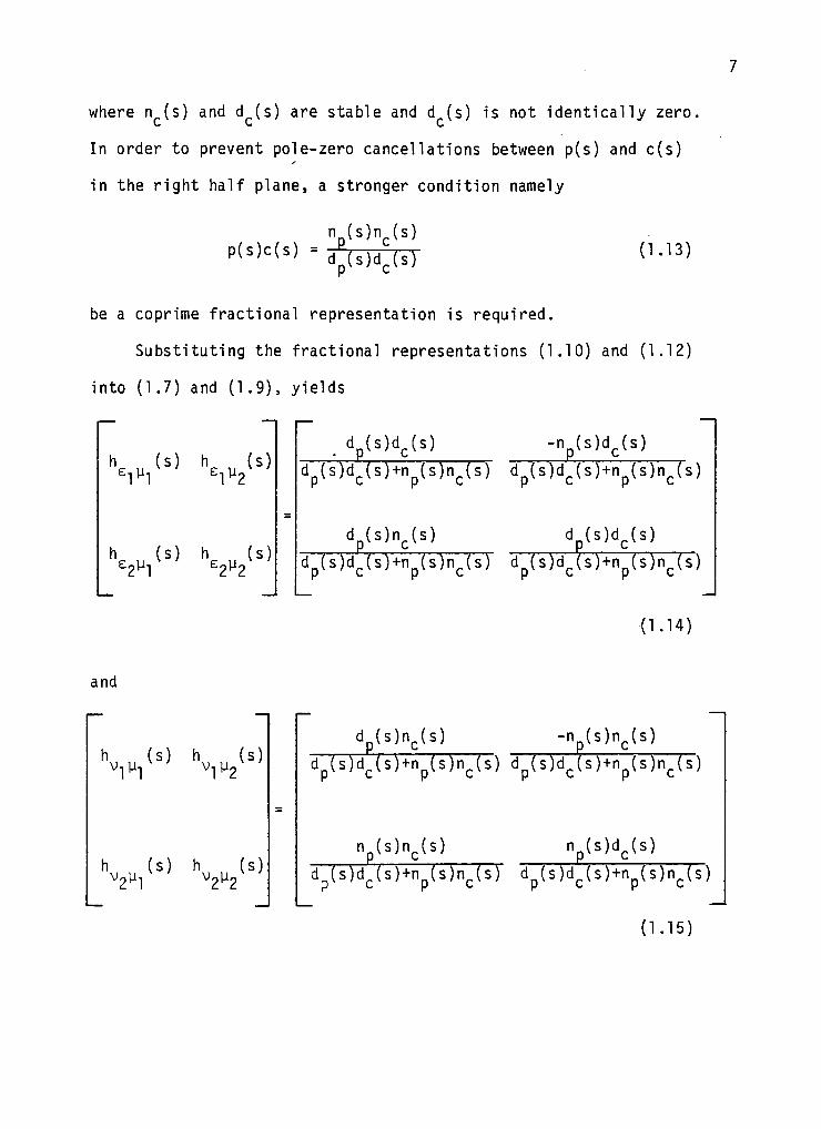
Substituting the fractional representations (1.10) and (1.12)

into (1.7) and (1.9), yields

h (s) h (s) ^1^2

h (s) h (s) e2yi ^2^2

. dp(s)d^(s) -np(s)d^(s)

dp(s)d^(s)+np(s)njs) dp(s)d^(s)+np(s)n^(s)

dp(s)n^(s) dp(s)d^(s)

dp(s)d^(s)+np(s)n^(s) dp(s)dJs)+np(s)n^(s)

(1.14)

and

h (s) h (s) ih

2h (s) h (s)

V2y2

dp(s)n^(s) -np(s)n^(s)

dp(s)d^(s)+np(s)n^{s) dp(s)dJs)+np(s)n^(s)

n (s)n^(s) n^(s)d^(s)

d (s)d^(s)+n (s)n^(s) d (s)d^(s)+n (s)n^(s)

(1.15)

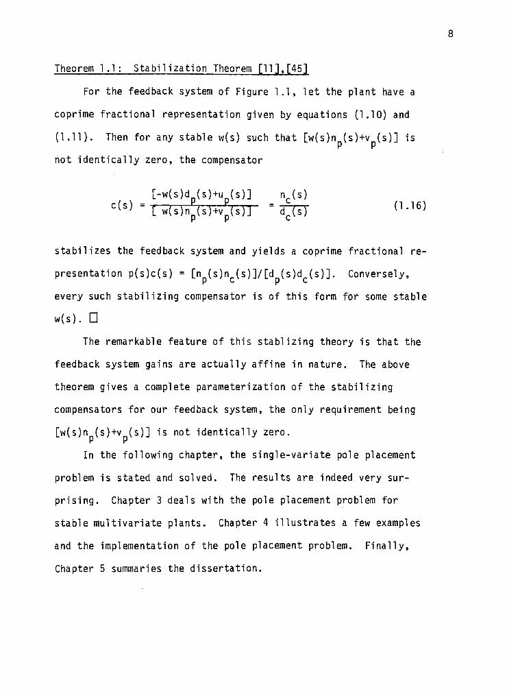
Theorem 1.1: Stabilization Theorem £11],[45]

For the feedback system of Figure 1.1, let the plant have a

coprime fractional representation given by equations (1.10) and

(1.11). Then for any stable w(s) such that [w(s)n (s)+v (s)] is

not identically zero, the compensator

[-w(s)d (s)+u (s)] n^(s)

'^'^ ~- Cw(s)np(s)+Vp(s)] = d-(lT ( - 6)

stabilizes the feedback system and yields a coprime fractional re­

presentation p(s)c(s) = [n (s)n (s)]/[d (s)d (s)]. Conversely,

p c p c

every such s tab i l iz ing compensator is of this form for some stable

w(s). D

The remarkable feature of this stabl iz ing theory is that the

feedback system gains are actually aff ine in nature. The above

theorem gives a complete parameterization of the s tab i l iz ing

compensators for our feedback system, the only requirement being

[w(s)n (s)+v (s ) ] is not ident ical ly zero.

In the following chapter, the single-variate pole placement

problem is stated and solved. The results are indeed very sur­

pr is ing. Chapter 3 deals with the pole placement problem for

stable mult ivariate plants. Chapter 4 i l lus t ra tes a few examples

and the implementation of the pole placement problem. Final ly,

Chapter 5 summaries the dissertat ion.

CHAPTER 2

THE SINGLE VARIATE POLE PLACEMENT PROBLEM

\lery often, establishing the closed loop system poles is of

fundamental importance. These poles are prescripted by the de­

signer - they may be the required cut off frequency for a filter or

the correct pole location for an aging plant. In many cases one

need not realize the exact transfer function while simultaneously

stabilizing the system. The resultant criterion may often be too

restrictive [4],[6] and hard to implement. One may prefer to work

in a less restrictive pole placement problem.

2.1 The Single Variate Pole Placement Problem:

In the pole placement problem we desire to find a stablizing

compensator such that the input-output transfer function takes the

form

where q(s) is a prescribed Hurwitz polynomial whose roots are the

poles that are to be placed and r(s) is an arbitrary numerator

polynomial which has no common factors with q(s). In order to

guarantee that h (s) has no poles at infinity it is required ^2^1

that the order of r(s) be less than or equal to the order of q(s).

Since q(s) is Hurwitz to ensure stability, any common factors

between r(s) and q(s) will be in the left half plane and must be

characterized by a polynomial coprimeness condition.

10

Consistent with the polynomial coprimeness concept, given a

plant p(s)

P ( s ) = 4 ^ ^ ^ (2.2) b'(s)b^(s)

we can construct

and

d (s) = b l l i K i l l (2.4) p m(s)

where m(s) is a Hurwitz polynomial character iz ing the poles of n (s)

and d ( s ) i a (s) and b (s) are Hurwitz polynomial charac ter iz ing

the s t r i c t l e f t - h a l f plane zeros of n (s) and d (s) respec t i ve ly ;

Y* Y*

whi le a (s) and b (s) are ant i -Hurwi tz polynomials character iz ing

the f i n i t closed r i g h t hal f -p lane zeros of n (s) and d (s) respec­

t i v e l y . Since n (s) and d (s) have no poles at i n f i n i t y

and

o(m) ^ o ( a b + o(a'^) ( 2 . 5 )

o(m) ^ o ( b b + o(b'") (2.6)

where o( ) denotes the order of the appropriate polynomial. Since

n (s) and d (s) are coprime, they cannot have a common zero at

s = «> and hence at least one of the i nequa l i t i es (2.5) or (2,6)

must be s a t i s f i e d wi th an equa l i t y . I f we l e t

k = |o(a'') + o(a^) - o(b'') - o ( b b | ( 2 . 7 )

then in the case of a striclty proper plant.

11

o(m) = o ( a b + o(a'") + k = o ( b ^ + o(b'") ( 2 . 8 )

or in the case of an improper plant,

o(m) = o ( a b + o(a'') = o(b^) + o(b'^) + k ( 2 . 9 )

Using the notation interduced, the following fundamental theroem

has been stated and proved. This theorm was originally stated by

Karmakolias [29], but later modified and proved by the author.

Theorem 2.1

Given p(s) there exists a compensator for the feedback system

of Figure 1,1 which stabilizes the system and yields

^j'^-'M 2h

where q(s) is a prescribed Hurwitz polynomial and r(s) is an

arbitrary polynomial such that o(r) ^ o(q), if and only if the

equation

a(s)a''(s) + 3(s)b"'(s) = q(s) ' (2,10)

admits polynomial solutions, a(s) and g(s), such that

0 ^ o(a) ^ o(q) + o(a^) - o(m) (2.11)

0 c 0(3) ^ o(q) + o(b^) - o(m) (2.12)

Proof: Sufficiency

If there exist polynomials a(s) and g(s) satisfying

a(s)a'^(s) + 3(s)b^(s) = q(s)

1^2

and (2.11) and (2 .12)^ def tne wt(£) 1^

w(s) = l i § M ^ . U ) . o l ^ l i n M . (3^ ( 2 : i 3 ) ) q(s)b^(s) ^ qLz)^is^ P-

Since q(s) and b (s) are bath- Hurwrtr palyntmsiails-afltK

o(qb ) i o(0m) v ta Z J Z .

This v e r i f i e s t ha t ^^^^""^^^ t s CE stcEUe rstioTtaJ functwrr . . Simt^'-q (s )h ' ( s )

l a r i l y the f a c t t ha t q(s) and s (s) a re bottj- HtiBw4tzitogethe*^with:'

(2.11) impl ies t ha t Q^^^l'pU) t^; ^ stabJg r^n'onarJ func t ion . Hence-j , q (s )a ' ( s )

w(s) i s a s tab le ra t i ona l ftmcttajr^ s±nffie i t is repues^fttsdr^as thfe '-

sum and products o f s tab le rattanaT furtctians:.

Using the w(s) def ined by ecpiSEttoir (2L-TX) to def ine arscoro*-

pensator f o r our system v ia the stabtTTzatrom thepotJewrwff^obta'tn'

the inpu t /ou tpu t t rans fe r function- h (s:) frour (1.15) and (1,16) < ^2^T

as

h (s) = -w(s)n fs )d (s) ^'U (s;)rr (s) (2.14) , V2y"! P r y H-

[ l a i s M s l ^ ( , ) . o L l M s L ( 3 ) 1 n ( s ) d - ( s ) . q ( s ) b ^ s ) P q(s,)ft^(s) P P P

+ u (s)n (s) p p

3(s)m(s)n (s)d (s)u (s) a(is)m(s)n (s)d5(s)v (s) P, B c — + 1:—pJi c

q ( s ) b ^ s ) q(s)a£(s)

^Up(s)np(,s)

13

Substituting (2,4) for d (s) in the first term and (2,3) for n (s)

in the second term of the above equation we have

3(s)b^(s)n (s)u (s) a(s)a''(s)d (s)v fs)

\^.^^'^ - - q(s) ' ' ' q(so' ' V,

+Up(s)np(s)

n„(s)uD(s) ais)a^{s)y(s)(iJs) - [q(s) - B(s)b'-(s)] - E L ^ j f — ^ ^ 3 ) '

Subs t i t u t i ng ( 2 . 9 ) ,

n J s ) u (s) ^ ot(s)a''(s)v (s)d (s) = a(s)a^(s) • ^ ^ ^ ^ ^ P P

. ^ i l ^ ln^isU^{s)..^{s)6^isn

Using (1 .11 ) ,

Y*

h f^\ - a(s)a (s) /« -,n\ ^ 2^1^^) - q(s) (^-^^^

To verify this is the required transfer function we must show that

o(r) ^ o(q). Using (2.5) and (2,11)

o(r) = o(a) + o(a )

^ o(a) + o(m) - o(a )

<; o(a) + o(a ) - o(m) + o(m) - o(a )

= o(q) (2,16)

14

This verifies that h (s) has no poles at infinity, completing the ^2^1

sufficiency or our proof.

Necessity:

Assume there exists a stable w(s) such that

^2y/^) = -w(s)np(s)dp(s) + Up(s)np(s) = (2.17)

Substituting (2.3) into (2,17) implies that

u (s) - w(s)d fs) = ^^!^'^^^}. - (2.18) P P q(s)a'^(s)a^(s)

Since u (s) - w(s)d (s) is stable while m(s), q(s) and a (s) are r r

Hurwitz polynomials, the anti-Hurwitz polynomial, a (s ) , in (2,18)

must be cancelled by a corresponding factor in r ( s ) . Hence (2.18)

implies there exists a polynomial a(s) such that

r (s) = a(s)a'^(s) (2.19)

Moreover, since u (s) - w(s)d (s) is stable and given by

u fs) - w(s)d (s) - d l M l l . (2.20) P P q(s)a^s)

it follows that,

o(a) + o(m) < o(q) + o(a )

implying

0(a) o(q) + o(ab - o(m) (2.21)

verifying (2.11).

15

Similiarly, it follows that equation (1.11) together with (2.17)

(2.19) and (2.4) that

vjs) + w(s)n (s) = ':q( ) -ffl(s)a'^(s)]m(s) ^2.22) P P q(s)b''(s)b'(s)

As before, since v (s) + w(s)n (s) is stable whi le q ( s ) , b (s) and r r

m(s) are Hurwitz i t fo l lows that there ex is ts a polynomial 3 ( s ) ,

such tha t

[q(s) - a ( s ) a ' ^ ( s ) ] = 3(s)b'"(s) (2.23)

which is the desired equa l i t y . Furthermore, since

v J s ) + w(s)n fs) = i l l M l l (2,24) P P q ( s ) b ^ s )

is stable, it follows that

o(3) < o(q) + o(b^ - o(m) (2,25)

verifying (2.12). This completes the proof to Theorem 2.1. Q

Furthermore if it is required that r(s) and q(s) be polynomial

coprime in Theorem 2.1, the following corollary is stated and proved,

Corollary 2,1

In Theroem 2.1, q(s) and r(s) are polynomial coprime if and

only if a(s) and 3(s) are polynomial coprime.

Proof:

Assuming a(s) and 3(s) are polynomial coprime, if

r(s) = a(s)a'"(s) and q(s) are not polynomial coprime, they have a

16

common zero at s = s^. Equation (2,10) implies that 3(s)b (s) also

has a common zero at s = s^. Since q(s) is Hurwitz, s = s must 0 TV ' ' Q

lie in the strict left-half plane, implying that it is actually

a common zero of a(s) and 3(s), since the zeros of a'"(s) and b' (s)

lie in the right half plane. This is impossible since a(s) and

3(s) are assumed to be polynomial coprime. Hence r(s) and q(s)

are polynomial coprime, completing the suffiency of the proof.

To verify the necessity, assuming r(s) and q(s) are polynomial

coprime, if s = s is a common zero of a(s) and 3(s), it is also

a common zero of r(s) = a(s)a'"(s) and q(s) = a(s)a'"(s) + 3(s)b'"(s),

which contradicts the initial assumption that r(s) and q(s) are

polynomial coprime. Hence a(s) and 3(s) are polynomial coprime,

completing the proof. Q

Consistent with Theorem 2.1 the solution to the pole placement

problem reduces to the solution of the linear polynomial equation

a(s)a"'(s) + 3(s)b"'(s) = q(s) (2.26)

subject to the constraints (2.11) and (2.12) which may be rewritten

as

i) o(a) ^ o(q) + o(a^ - o(m) (2.27)

ii) 0(3) < o(q) + o(b^ - o(m) (2.28)

iii) o(m) ^ o(q) + o(a^) (2.29)

iv) o(m) € o(q) + o(b^) (2.30)

Equations (2.29) and (2.30) are obtained from the fact that

a(s) and 3(s) are polynomials that is o(a) ^ 0 and 0(3) ^ 0.

17

Equation (2.25) represents o(q) + 1 equations in o(a) + 0(3) + 2

unknowns, and for a solution we require the generically necessary

condition

o(q) + 1 ^ o(a) + 0(3) + 2 (2.31)

2.2 Proper and Strictly Proper Plants:

Recall from equation (2.8), which states

o(m) = o(a^ + o(a^) + k = o(b^) + o(b'')

For a solution to the pole placement problem, we require the equa­

tions (2.31), (2.27), (2.28), (2.29), (2.30) and (2.8) to be

satisfied simultaneously.

Substituting equations (2.27), (2.28) and (2.8) we have

o(q) + 1 ^ [o(q) + o(a^ - o(m) + o(q) + o(b^) - o(m)] + 2

= 2o(q) - o(a'') - o(b'') - k + 2

or equivalently

o(q) ^ o(a'') + o(b' ) + k - 1 (2.32)

Now, equations (2.32) and equations (2.29) and (2.3) have to

be satisfied simultaneoulsy. Substituting equations (2.8) in (2.29)

and (2.30) we have

o(q) > o(a'') + k (2.33)

and

o(q) ^ o(b' ) (2.34)

18

Consider the following cases:

Y* Y*

Case 1: o(b ) 1 and o(a ) + k 1. Equation (2.32) states

o(q) ^ [o(a'^) + k] + o(b'') - 1

Since o(b'") - 1 ^ 0 because o(b'^) 1, (2.32) implies

o(q) ^ o(a'^) + k. Hence (2.33) is satisfied. Since 0(3"^) + k 1,

0(3"^) + k - 1 0, and (2,32) implies

o(q) >. o(b'')

and hence (2.34) is satisifed.

Y* Y*

Hence under the conditions o(b ) : 1 and o(a ) + k 1, the

condition for the solution of the pole placement problem is (2,32),

Case ii: o(b'^) = 0 and o{a.^) + k 1. In this case (2.32), (2.33) and (2.34) reduce to

i) o(q) ^ o(a'") + k - 1

ii) o(q) ^ 0(3" ) + k

iii) o(q) ^ 0

respectively

iii) is satisifed by i), since o(a ) + k 1, for i) and ii) to be Y*

simultaneously satisfied o(q) ^ o(a ) + k. y Y*

Hence under the condition o(a ) + k ; 1 and o(b ) = 0, which

referes to a stable plant, the condition to solve the pole place­

ment problem is

o(q) ^ 0(3"") + k

Case iii: o(b'^) 1 o(a''') + k = 0. Since both o{a^) and k are

positive integers greater than or equal to zero o(a ) + k = 0 implies

19

0(3* ) = 0 and k = 0. In this case (2.32), (2.33) and (2.34) reduce

to

i) o(q) >. o(b'') - 1

ii) o(q) > 0 Y*

iii) 0(q) ^ 0(b ).

Y*

Since o(b ) : 1, ii) is satisfied by i). For i) and iii) to be

satisfied simultaneously satisfied, 0(q) o(b ). Hence under the Y* y»

condition o(b 0 ^ 1 and o(a ) + k = 0, which refers to a proper

unstable plant with no r ight -ha l f plane zero's, the condition to

solve the pole placement problem is o(q) s o(b ).

Case i v : o(b"^) = 0 and 0(3^ ) + k = 0. Equations (2.32), (2.33)

and (2.34) reduce to

o(q) ^ -1

o(q) ^ 0

o(q) ^ 0

respectively. Since q(s) is polynomial, the solution to the pole

placement problem for a stable mini phase plant is

o(q) ^ 0.

2.3 Improper Plants

For improper plants equation (2.9) states that

o(m) = o(ab + o{d^) = o(bb + o(b'') + k.

For the solution to the pole placement problem we require

equations (2.32), (2.29), (2.30) and (2.9) to be satisfied simul­

taneoulsy. Substituting (2.9) in (2.29) and (2,3) we have

20

o(q) ^ 0(3*") (2,35)

o(q) ^ o(b'") + k (2.36)

Consider the following cases:

Case i: 0(3"") ^ 1, o(b'^) + k ^ 1.

By similar arguments of case i of the previous section, the condition

for the solution of the pole placement problem is

o(q) ^ 0(3"") + o(b'') + k - 1

Case ii: 0(3*^) = 0 and o(b'') + k ^ 1

Again using similar agruments of case ii in the previous section,

the condition for the solution to the pole placement problem is

o(q) ^ o(b"') + k.

The above cases for the proper and improper plants yields

necessary and sufficient conditions for the linear equation (2.10)

to be generically solvable. Indeed, the polynomial coprimeness of

a' (s) and b' (s) implies that (2.10) will always admit coprime

solutions when the above mentioned cases are satisfied. The

equation (2.10) may also admit solutions which are not polynomial

coprime. On the other hand if any one of the cases are not

satisfied, the pole placement problem is generically unsolvable

though it may admit solutions for certain q(s) which lie in an

appropriate lower dimension subspace.

Finally denote the integer [0(3"") + o(b'^) + k] by n(p) which

represents the total number of closed right-half plane poles and

21

zeros of the plant. Indeed, 0(3"^) is precisely the number of

finite closed right half plane zeros of p(s), while o(b'^) is the

number of right-half plane poles of p(s) and k represents the

number of poles or zeros at infinity (depending on whether (2.8)

or (2.9) holds). Il(p) is a natural measure of the degree by which

p(s) fails to be miniphase. Consistent with the above, we can

state the following theorem.

Theorem 2.2: Pole Placement Theorem

Given p(s) there exists a compesnator for the feedback system

of Figure 1.1 which stabilizes the system and yields

v^y/ q(s) 2 1

where q(s) is a prescribed Hurwitz polynomial, r(s) is an arbitrary

polynomial such that o(r) : o(q), if

o(q) ^ n(p) - 6

where 6, the pertubation factor is either 0 or 1 as indicated by

Table 2.1. Conversely if o(q) < n(p) - 5, the pole placement prob­

lem is generically unsolvable.D

2.4 Parameterization of Solution Space

In this section the parameterization of the solution space for

the pole placement problem is discussed. It follows from Theorem

2.1, that the space of compensators which resolve the pole placement

problem for a given q(s) take the form

22

TABLE 2 . 1 : Perturbat ion factor ' 6 ' fo r s ing le var ia te pole

placement problem.

P(s)

Proper

P(s)

Improper

6 = 1

k + 0(3"") ^ 1

and

o(b'") ^ 1

k + o(b'") ^ 1

and

0(3"^) ^ 1

6 = 0

k + 0(3"^) = 0

or

o(b'') = 0

0(3'') = 0

23

[-w(s)d (s) + u (s)]

'^'^ ~- Lw(s)np[s) . Vp(s)] ^2.37)

where w(s) is given by (2.13) with a(s) 3nd 3(s) chosen to

S3tisfy (2.11) and (2,12), together with the condition that

[w(s)n (s) + V (s)] is not identic3lly zero.

If aP(s) snd 3 (s) represent a p3rticul3r solution 3nd a (s)

snd 3 (s) represent homogeneous solutions to equation (2,10), the

entire solution space takes the form

a(s) = aP(s) + a^s) (2.38)

3(s) = 3P(s) + 3^s) (2.39)

where aP(s) and 3 (s) satisfy

aP(s)a^(s) + 3P(s)b^(s) = q(s) (2.40)

aP(s) 3nd 3P(s) are particular solutions computed in Theorem 2.2.

a (s) and 3 (s) satisfies

a^s)a"'(s) + 3^s)b''(s) = 0 (2.41)

I f j ( s ) i s an a r b i t r a r y polynomial, we can pick

a ^ s ) = j (s)b '^(s) (2,42)

and

3 ^ s ) = - j ( s )3 ' " ( s ) (2.43)

(2.42) 3nd (2.43) are homogeneous solutions since they S3tisfy (2.41)

24

In order to show (2.42) 3nd (2.43) characterize all the homo­

geneous solutions let a(s) and g(s) be arbitrary homogeneous

solutions. Since (2.42) and (2.43) are homogeneous solutions, they

satisfy (2.41) namely

a(s)a'"(s) + B(s)b"'(s) = 0. (2.44)

pTtking j(s) = ^ ^ (2.45) b' (s)

-j(s)a^(s) =--fll)-a^(s) b' (s)

= - ^ b ^ ( s ) b' (s)

= B(s) (2.46)

which is in the form (2.43) wi Y*

Since a (s) and b (s) are polynomial coprime, there exist poly­

nomials x(s) and y(s) such that

a''(s)x(s) + b"^(s)y(s) = 1. (2.47)

Mult iplying (2.45) by (2.47)

j ( s ) = - | ^ [a'"(s)x(s) + b'^(s)y(s)] b'^(s)

substi tut ing (2.44) and simplifying

( S ) = . M l i b ^ i s M l i . y ( s ) a ( s )

b'^(s)

25

= -B(s)x(s) + y(s)a(s)

Hence j(s) is polynomial, since it has been expressed as sums and

products of polynomials.

Hence the above arguments conclude that the entire solution

space of (2.10) takes the form

a(s) = aP(s) + j(s)b'"(s) (2.48)

and

3(s) = 3^(5) - j(s)a''(s) (2.49)

where j(s) is an arbitrary polynomial. In the pole placement prob­

lem, however, the subset of the solution space that satisfies the

constraints. (2.11) and (2.12) of Theorem 2.1 is required. Assuming

that aP(s) and 3P(s) satisfy (2.11) snd (2.12), the constrsints on

the order of j(s) S3tisfying (2.11) 3nd (2.12) is required.

In the case of a proper pl3nt recall (2.8),

o(m) = o(a^) + 0(3"") + k = o(bb + o(b'^).

By substituting (2.8), o(a) = o(j) + o(b" ) 3nd 0(3) = o(j) +

o(a''), (2.11) and (2.12) reduce to

o(j) ^ o(q) - 0(3'') - o(b"') + k

o(j) ^ o(q) - 0(3" ) - o(b'^).

3nd

o(j) ^ 0.

26

In order for the above three conditions simultaneously

o(j) ^ o(q) - 0(3" ) - o(b" ) - k + 6

Recall 0(3' ) + 5(b' ) + k is the qu3ntity IT(P), the above inequality

may be rewritten 3S

o(j) ^ o(q) - IT(P) + 6. (2.50)

where '6' is the pertub3tion fsctor is either 0 or 1 snd is given

by Table 2.1.

Similarily in the C3se of 3n improper plant recall (2.9)

o(m) = 0(3^) + 0(3^) = o(b^) + o(b'') + k

Ag3in substituting (2.9), e(a) = o(j) + o(b'') snd 0(3) =

o(j) + 0(3''). (2.11) snd (2.12) reduce to

o(j) ^ o(q) - o(a^) - o(b^)

o(j) < o(q) - 0(3"") - o(b'') - k

snd

o(j) 3 0.

In order for the sbove three constraints to be satisfied simul­

taneously,

o(j) ^ o(q) - n(p) + &

where '5' the pertubation factor is given by Tsble 2.1. We msy

psrsmeterizstion the solution spsce for the pole plscement prob­

lem vis:

27

Corollary 2.2:

Let p(s) and q(s) be given and le t aP(s) and aP(s) be solutions

of equation (2.10) such that 0 < o(aP) ^ o(q) + o(a ) - o(m) snd

0 ^ 0(3P) ^ o(q) + o(b ) - o(m). Then the set of compensstors which

resolve the pole plscement problem tske the form

[-w(s)d (s) + u (s) ]

"^ ' ^ ^ [w(s)nWs) +vWs)]

where

, ( s ) = r3P(s), - j(s)a^(s)]m(s) .^^

[q(s)b ' (s) ] P

. fgPfs) ^ •i(s)b"(s)]m(s) ^ ^^^

[q(s)3^(s)] P

where j ( s ) is sn srb i t rs ry polynomisl such thst

o( j ) ^ o(q) -[TT(P) - 6]

and is chosen such that [w(s)np(s) + Vp(s)] is not identical ly

zero '5 ' is the pertubation factor given by Table 2 .1 . D

CHAPTER 3

THE STABLE MULTIVARIATE POLE PLACEMENT PROBLEM

In the first section of this chapter, the multivariste frsc-

tionsl representstion theory [57],[58] will be formulated. In the

ensuing sections the stable multivariste pole placement problem

will be formulated and solved.

3.1 Mulitvariste Frsctionsl Representstion Theory

This slgebrsic theory [11] is set in s nest of rings, groups

snd multiplicstive structures

G 3 H 3 I O J.

Here, G is s ring with identity which represents the feedbsck

system snd its subsystems snd H is s subring of G contsining the

identity which models the systems which sre stsble in some sense.

The compensstor will be chosen so thst the oversll system will be

represented by sn operstor in the subring H. Finslly, I denotes

the mulitplicstive set composed of elements of H which sdmit sn in­

verse in G while J denotes the multiplicstive subgroup of I msde

up of elements which sre invertsble in H. Detailed examples of

the axiomatic structure, {G,H,I,J} are given in reference [11]

and will not be repeated here.

P has a right frsctionsl representstion in {G,H,I,J} if

P = N D " (3.1) pr pr

where N e H snd D e l . Furthermore, we ssy thst this pr pr

28

29

is right coprime [28] if there exist U snd V in H such thst

U N + V D = 1 (3.2) pr pr pr pr ^ '

This equslity is equsl to the clsssic3l coprimeness concept for

rstionsl functions snd mstrices while being well defined in our

general ring theoretic setting. In particulsr, if G is the ring

of rstionsl functions snd H is the ring of polynomisls (3.2)

implies thst N snd D hsve no common zeros; snd if G is the ring pr pr

of rstionsl functions snd H is the ring of exponentislly stsble

rstionsl functions, (1.2) implies thst N snd D hsve no common pr pr

r i g h t - h s l f plsne zeros.

Since the r i ng G i s , in geners l , non-commutstive we slso de­

f i n e 3 l e f t f r s c t i o n s l representst ion of P vi3 the equs l i t y

P = Dp^-^Np^ (3.3)

where D , e H snd N •• e I . Furthermore, t h i s representst ion is

l e f t coprime [28] i f there ex is t Up-j snd Vpi in H such ths t

^i%i ' ^^^^ - ' (3.4)

In the clsssicsl esse of 3 rstionsl functions or matrices these

fractional representations sre sssured to exist. However, this is

not the esse in the genersl ring theoretic setting. Therefore, for

distributed, time-vsrying snd multidimensionsl systems we sssure

thst our plsnt sdmits such a representstion ss s prerequisite to

the theory.

30

Since H represents s ring of stsble systems we ssy that the

feedback system of Figure 1.1 is stable if sll its internsl snd

externsl gsins sre elements of H. By using the above described

fractional representation theory a solution to the stabilization

problem was obtained in reference [11]. In particular, if the

plant P is given by P = D^" N ,, the the compensator

C = (WNpi+Vp^)-^-WDp^.Up^) (3.5)

stabilizes the feedback system for any W H such that (WNp,+Vp )el;'

and every stabilizing compensator is given by (3.5) for some

WeH. Moreover, this compensstor is used in the feedbsck system of

all the usual gains of the closed loop system are linear (actually

affine) in W. Specifically, the System's input/output gain is

given by

H,, ,, = 1 + N WD 1 + N U v_y, pr pi pr pr

The remaining gains are also linesr in W snd sre derived in reference

[11].

3.2 The Stsble Pole Plscement Problem

In the stsbilization theory discussed in the previous section

it was assumed that the plant admitted both left and right coprime

fractionsl represent3tions

p(s) = v(^)v" ' (^) = %r'(^)%i(s) (3.6) for which there exist U e H snd V e H such thst

31

U (s)N (s)+V (s)D (s) = I pr pr pr pr

3nd U 1 £ H snd V , e H such thst pi pi

lpT(s)Up^(s)+Dp^(s)Vpi(s) = I

(3.7)

(3.8)

Since s doubly coprime frsctionsl representstion exists when­

ever sepsrste left snd right coprime frsctionsl representstions

exist, we msy work with s doubly coprime frsctionsl representstion

without loss of generslity. This, in turn, mesns thst rsther thsn

three equslities (3.6) through (3.9), we hsve eight equalities with

which to msnipulste the feedback system equations. These eight

equstions csn be written ss follows:

pr

pr

snd

•NpT(s)

-U pl

'pl

pr

^1

V^^^ %r( )

^l(^)

pr

Pl

V ' "V ^

V^^^ 'pl ' 0

(3.9)

I

(3.10)

For the pole plscement problem, we hsve considered s stsble

rstionsl multivsriste plsnt chsrscterized by sn n by n trsnsfer

function mstrix P(s). Since P(s) is stsble, it admits a trivial

rational fractional representation with

32

Np^(s) = Np^(s) = P(s) (3.11)

and

^r^^) = %l(^) = ^ (3.14)

The stablizing compensator given by (3.5) reduces to

C(s) = (W(s)P(s)+I)"'' (W(s)) (3.15)

and the input/output gain given by equation (3.6) reduces to

H (s) = P(s)W(s). (3.16)

2h

Here W(s) is a stable rational matrix.

In this highly specialized multivsriste esse we formulate the

pole placement problem by requiring that W(s) be chosen to stabilize

the system and yield sn input/ouput gsin of the form

where q(s) is the prescribed Hurwitz polynomisl whose roots are

the poles that are to be placed and R(s) is an arbitrary n by n

polynomial matrix such that

o(R) ^ o(q). (3.18)

where the order of a matrix is defined to be the maximum of the

orders of its elements.

33

Given the plant P(s), a common Hurwitz denominator bCs) is

factored out. The numerator is then transformed into the Smith

Canonical form [28]. After replacing the common denominator the

resultant matrix form yields the Smith-Macmillan form [28] for

P(s) of (3.11).

P(s) = U(s)D(s)V(s) (3.19)

where U(s) and V(s) are unimodular polynomial matrices and D(s)

is a diagonal matrix with rational entries d.(s) as in equation

(3.20)

a^(s) a. (s) d.(s)=-! T-! , i = l , 2 , n. (3.20) ' b](s)

Y*

In equation (3.20), a.(s) are polynomials whose roots are in the

right-half plane (anti-Hurwitz) and a.(s) and b.(s) are polynomials

that are Hurwitz. Since D(s) is a diagonal matrix, it may further

be written as the product of three diagonal matrices as follows:

D(s) = A[^(S)B^_-''(S)AL(S) (3.21)

Here the diagonal entries of An(s) are the polynomials

r -1 1

a.(s), i = l,...,n, B, (s) are the polynomials b.j(s), i = l,...,n

and A. (s) are the polynomials a.(s), i = 1,2,...,n. Hence, after

all the above transformations the plant P(s) can be written as

P(s) = U(S)AP(S)BL"''(S)AL(S)V(S) (3.22)

34

Letting V.(s) denote the ith row of V(s) we then obtain the

following theorem.

Theorem 3.1: Stable Pole Placement Theorem.

i) If the stable multivariate pole placement problem ad­

mits a solution then

o(q) o(bl) - o(al) - o(V.) (3.22)

for all i = 1,2 n.

ii) The stable multivariate pole placement problem admits a

solution if

o(q) >. o(b]) - o(al) (3.23)

for all i = 1,2 n.

Proof:

i) Let there exist a stable W(s) such that

H (s)=-P(s)W(s)=^R(s)

Substituting for P(s), using equation (3.22) we obtain

-U(S)A^(S)BL"^S)AL(S)V(S)W(S) = - ^ R ( S ) . -

The above equation implies there exists a matrix a(s) such that

N^(s) a(s) = R(s) (3.23)

where

N^(s) - U(s)Ap(s) (3.24)

35

and

a(s) = -q(s)BL-''(s)AL(s)V(s)W(s) (3.25)

From equation (3.24) we can obtain

W(s) = - - ^ V''(s)AL"^(s)BL(s)a(s). (3.26)

In equation (3.23) R(s) is a polynomial matrix by definition and

Nn(s) is a polynomial matrix by construction. Hence, for the pro­

duct N(s)a(s) to be a polynominal matrix, the poles of the elements

of a(s) should cancel the zeros of the elements of Nn(s). This

is impossible as Nn(s) has zeros in the right half plane where as

a(s) has its poles in the left half plane, if it has any. Hence

for the product Np(s)a(s) to be polynomial, a(s) has to be polynomial.

Since W(s) is stable, using equation (3.25),

o(a.j) = o(q) - o(bl) + o(al) + max {o(vJ) + o{^.)} (3.27) J

Here the superscript j refers to the jth column of the matrix and the

subscript i or j refers to the respective rows. Since,

max {o(V'?) + o(W.)}^ max (V^) + max o(W.) ^ o(V.) + o(W.) (3.28) j ^ " j j ^ '^

and W(s) is stable o(W.) ^ 0 and hence (3.27) reduces to the <J

inequality

o(a.) ^ o(q) - o(b]) + o(a]) + o(V.)

Since a(s) is a polynomial matrix

o(a-) ^ 0 and hence

35

0 ^ o(q) - o(b]) + o(a]) + o(V.)

which implies

o(q) ^ o(bl) - o(a]) - o(V.),

for all i = 1,2 n.

Thus proving (i) and completing the necessity of the proof,

ii) It is given that

o(q) ^ o(bl) - o(al), i = 1,2, n. (3.23)

Let W(s) be defined by the following equality

W(s) = - - ^ l\[\s)B^_{s)

By the above def in i t ion of W(s), W(s) is a diagonal rational matrix

whose elements are given by

m. m b|(s) V ^ ^ ^ V . ^ ^ ^ ^ ^ 0

q(s)a.(s) n. n. , y s + y s + + y

" i i-1 °

i = 1,2 ,n (3.29)

Let K(s) be a diagonal polynomial matrix whose elements are given

by

• n. n.-m. K,(s) = r-^i ^ ^ . i = 1.2, ,n. (3.30) ^ ^m.

1 Defining W(s) by

W(s) = V"^s)W(s)K(s)V(s) (3.31)

37

not noting that the

Lt W(s) = Lt V"^s)K(s)W(s)V(s) = 1 (3.32)

S-H» S-x»

where I is the identity matrix. Using (3.23) and (3.32), W(s) is

guaranteed to be stab .e at S = "s. Thus W(s) is a stable rational

matrix and is given by

W(s) = V-''(s)W(s)K(s)V(s) = -V-^s) ^ A L " ' ' ( S ) B | _ ( S ) K ( S ) V ( S )

Now to check if the above stable W(s) gives us the required input/

output trsnsfer function

H^ „ (s) = -P(s)W(s)

2n

= -[U(s)Ap(s)B,-^(s)A, (s)V(s)]

[_V-''(s)i7—\ (S)BL(S)K(S)V(S)]

= •^U(s)A^(s)K(s)V(s)

= - ^ R ( s ) (3.33)

which is the required trsnsfer function. R(s) = U(s)A|^(s)K(s)V(s)

is s polynomisl mstrix since U(s) ,Aj^(s),K(s) and V(s) sre all

polynomial matrices by construction. This completes the proof.Q

The necessary and sufficient conditions of (3.22) and (3.23)

do not coincide except in the single variate case where they

shown in Theorem 2,2. The above theorem leaves many unanswered

questions. In particular, since the Smith form is not unique.

38

the necessary condition can be tightened by varying the Smith form.

These aspects will be discussed further in Chapter 5.

CHAPTER 4

EXAMPLES

In this chapter examples of both single variate and multivariate

pole placement problems are presented. These examples highlight the

simplicity and powerfulness of the fractional representation theory,

especially the pole placement problem.

Example 4.1: Unstable Proper Plant

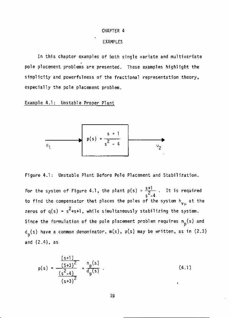
Figure 4.1: Unstable Plant Before Pole Placement and Stabilization.

s+1 For the system of Figure 4.1, the plant p(s) = —^— . It is required

s -4 to find the compensator that places the poles of the system h at the

2 zeros of q(s) = s +s+l, while simultaneously stabilizing the system.

Since the formulation of the pole placement problem requires n (s) and

d (s) have a common denominator, m(s), pCs) may be written, as in (2.3)

and (2.4), as

p(s) =

(s+1)

(S+3)'

(s^-4)

(s+3)'

C4.1)

39

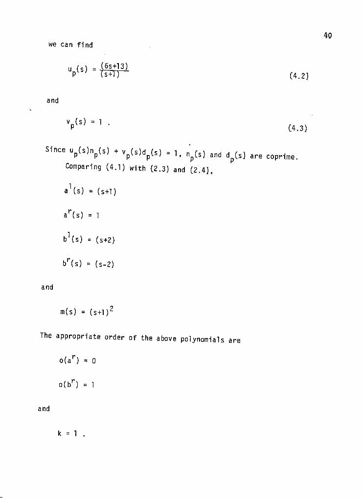
40 we can find

u (s) - (6S+13)

and

^P^^^ ~- ' • C4.3)

Since Up(s)np(s) + Vp(s)dp(s) = 1. PpCs) and dpCs) are coprime.

Comparing (4.1) with (2.3) and [2.4),

a^(s) = (s+1)

a^(s) = 1

b^s) = (s+2)

b''(s) = (s-2)

and

m(s) = (s+1)^

The appropriate order of the above polynomials are

0(3"") = 0

o(b'^) = 1

and

k = 1 .

41

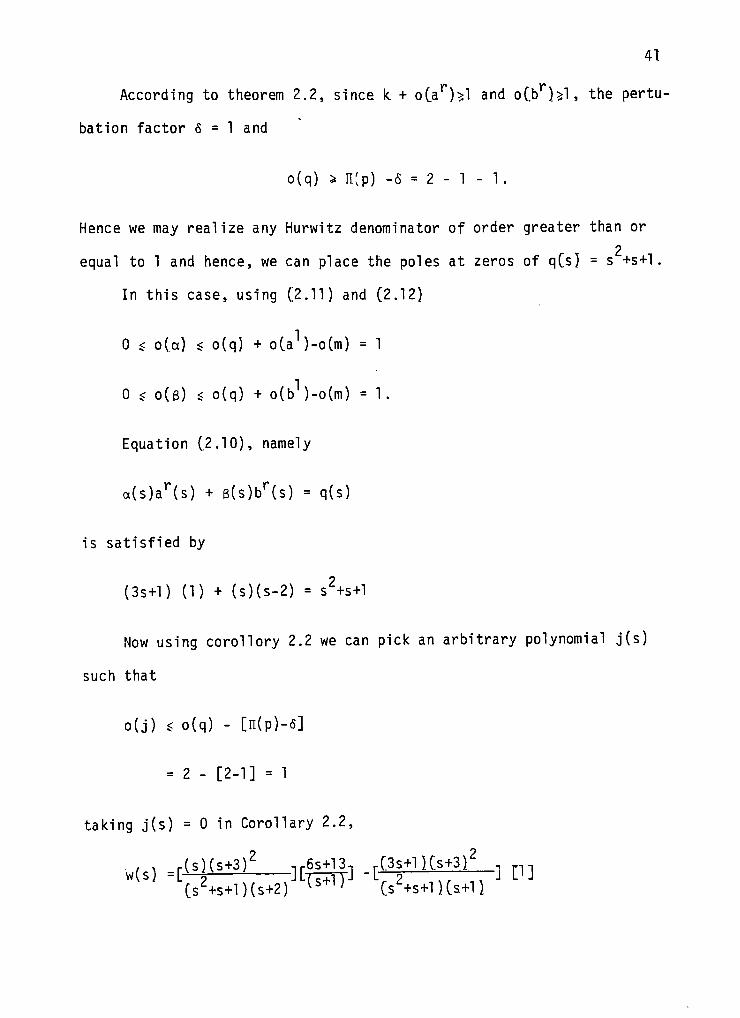
Y* Y*

According to theorem 2.2, since k + oCa )5l and oCb )5l, the pertu­

bation factor 6 = 1 and

o(q) ^ n(p) - 6 = 2 - 1 - 1.

Hence we may realize any Hurwitz denominator of order greater than or 2

equal to 1 and hence, we can place the poles at zeros of qCs) = s +s+l.

In this case, using [2.11) and (2.12)

0 ^ o[a) $ o(q) + o[a )-o[m) = 1

0 $ O(B) $ o(q) + o(b^)-o(m) = 1.

Equation [2.10), namely

a(s)a' '(s) + e(s)b'^[s) = q(s)

is satisfied by

(3s+l) (1) + (s)(s-2) = s^+s+1

Now using corollory 2.2 we can pick an arbitrary polynomial j ( s )

such that

o(j) ^ o(q) - [n(p)-6]

= 2 - [2-1] = 1

taking j (s ) = 0 in Corollary 2.2,

/ A r(s)(s+3)^ -,r6s+13-, [3s+l)[s+3}^ , , w(s) =i^'-k^ iil\+-\ U "L~~2 TT ^ J LU

[s^s+l)(s+2) '^^^^' [sSs+l)[s+l l

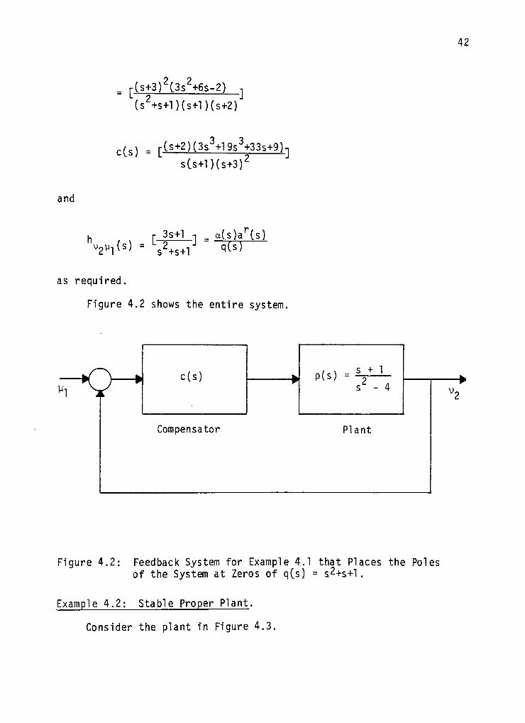
42

and

r[s+3)^[3s^+6s-2) ..

(s^+s+l)(s+l)(s+2)

c[s) = [(s+2)(3s3+19s3+33s+9)-j

s[s+l)(s+3)^

h r ^ l ± L i - "(.s)a''(s) V l ( ^ ) - s2,s+l ^^^^~~

as required.

Figure 4.2 shows the entire system.

> - * c(s)

Compensator

h w

P(s) - V ' s^ - 4

Plant

w

^2

Figure 4.2: Feedback System for Example 4.1 that Places the Poles of the System at Zeros of q[s) = s^+s+l.

Example 4.2: Stable Proper Plant.

Consider the plant in Figure 4.3,

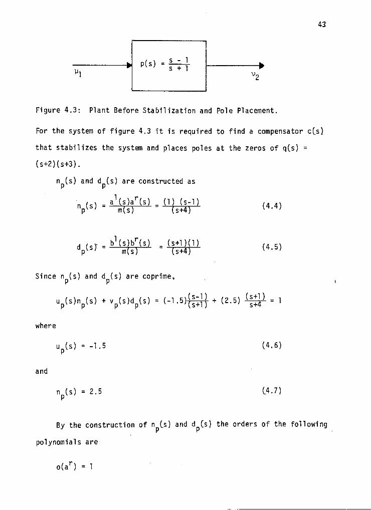
43

yi P(s) = - s - 1

s + 1 V,

Figure 4.3: Plant Before Stabilization and Pole Placement.

For the system of figure 4.3 it is required to find a compensator c[s)

that stabilizes the system and places poles at the zeros of q[s) =

(s+2)(s+3).

n (s) and d (s) are constructed as

n fO - aHs)a'^(s) _ (1) (s-1) "p('^ - ~i(?) (s+4) (4.4)

H ro- - b^(s)b';(s) _ (s+l)(l) ''p^'^ i m - (s+4)

(4.5)

Since n (s) and d (s) are coprime.

u (s)n (s) + V (s)d (s) = (-1.5)i|^ + (2.5) -^^p- = 1 P P P P UTTJ s+4

where

Up[s) = -1.5 (4.6)

and

np[s) = 2.5 [4.7)

By the construction of n [s) and d [s) the orders of the following

polynomials are

oia'') = 1

44

o[b'') = 0

and

k = 0.

According to Theorem 2,2, since k + o[a'")5l and o[b^) = 0, the pertuba­

tion factor 6 = 0 and

o(q) >. n[p) - 6 = 1 - 0 = 1.

Hence we can realize any Hurwitz denominator of order greater than

or equsl to 1 and hence, we can place the poles at the zeros of q(s) =

(s+2)(s+3).

In this case, using [2.11) and [2.12)

0 $ o(a) ^ 2 + 0 - 1 = 1

and

0 < o[e) $ 2 + 1 - 1 = 2

Equation [2,10) which requires

a(s) a''(s) + 6(s) b' [s) = q(s)

is satisfied by

a(s) = [s+6)

and

6(s) = (12)

45

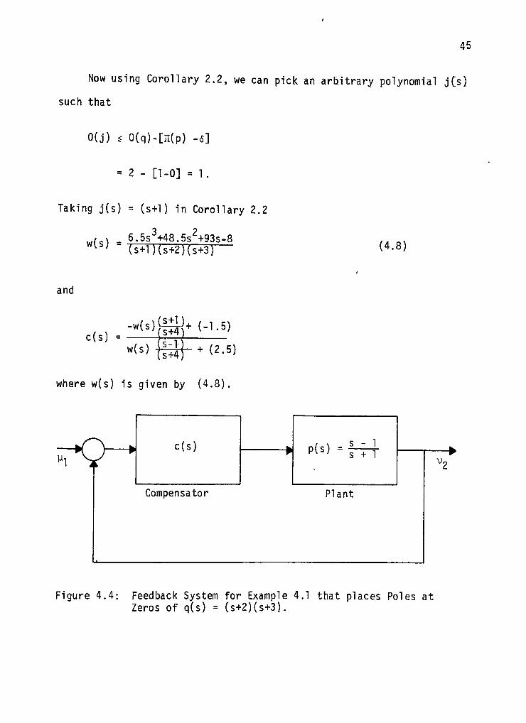
Now using Corollary 2.2, we can pick an arbi t rary polynomial j [ s )

such that

0( j ) .< 0[q)-[n(p) -6]

= 2 - [1-0] = 1 .

Taking j ( s ) = (s+1) in Corollary 2.2

w(s) 6.5s'^+48.5s^+93s-8 (s+l)(s+2)(s+3) (4.8)

and

c(s, = :!i!lpli:l:!' w(s)||^M2.5)

where w(s) is given by (4.8).

Compensator Plant

Figure 4.4: Feedback System for Example 4,1 that places Poles at Zeros of q[s) = [s+2)(s+3).

46

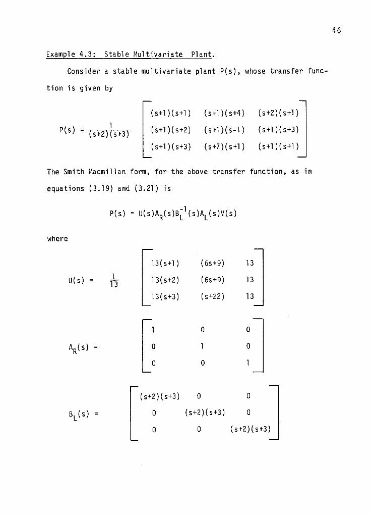
Example 4.3: Stable Multivariate Plant.

Consider a stable multivariate plsnt P(s), whose transfer func­

tion is given by

''(^^ = (s+2)(s+3)

(s+l)(s+l) (s+l)(s+4) (s+2)(s+l)

(s+l)(s+2) (s+l)(s-l) (s+l)(s+3)

(s+l)(s+3) (s+7)(s+l) (s+l)(s+l)

The Smith Macmillan form, for the above transfer function, as in

equations (3.19) and (3.21) is

,-1 P(s) = U(s)A^(s)B['(s)Ajs)V(s)

where

U(s) = Jj

A„(s) -

13(s+l)

13(s+2)

13(s+3)

1

0

0

(6s+9)

(6s+9)

(s+22)

0

1

0

13

13

13

0

0

1

BL(S)

(s+2)(s+3) 0 0

0 (s+2)(s+3) 0

0 0 (s+2)(s+3)

47

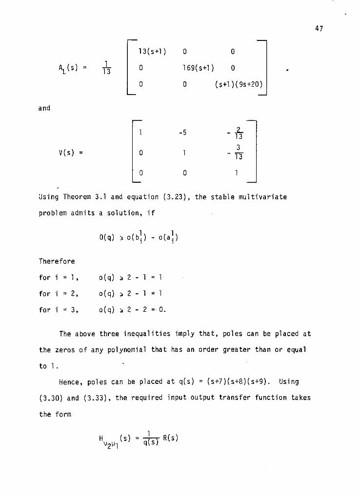
AL(S) = iV

13(s+l) 0 0

0 169(s+l) 0

0 0 (s+l)(9s+20)

and

V(S) =

1 -5

0 1

0 0

2-13

_3_ 13

1

Using Theorem 3.1 and equation (3.23), the stable multivariate

problem admits a solution, if

0(q) >. o(b]) - o(al)

Therefore

for i = 1 ,

for i = 2,

for i = 3,

o(q) ^ 2 - 1 = 1

o(q) ^ 2 - 1 = 1

o(q) ^ 2 - 2 = 0 .

The above three inequalities imply that, poles can be placed at

the zeros of any polynomial that has an order greater than or equal

to 1.

Hence, poles can be placed at q(s) = (s+7)(s+8)(s+9). Using

(3.30) and (3.33), the required input output trsnsfer function tskes

the form

H (s)=^R(s) 2 1

where

and

q(s) = (s+7)(s+8)(s+9)

48

R(s) = ^

13s^(s+l) 13s^(s+4) -s^(2s+29)

13s^(s+2) 13s^(s- l ) -s^(2s+31)

13s^(s+3) 13s2(s+7) -2s2(s+72)

CHAPTER 5

CONCLUDING REMARKS

A new approach, using the fractional representation theory, to

the Pole Placement Problem was proposed. The starting point for the

theory rests with the celebrated 1976 papers of Youla, Bongiorno and

Jabr [57],[58] in which a complete parameterization of the set of

stabilizing compensators for a general multivariate system was first

formulated. Of course, such parameterizations have long been known

in the single variate case, while several authors have several altern­

ate formulations [1],[4],[8],[17],[38],[39],[51],[60]. Although the

YBJ theory was formulated using a polynomial fractional representa­

tion [57],[58], it was soon discovered that the theory could be simpli­

fied and generalized by working with stable factors rather than poly­

nomial factors. This in turn led to both distributed 7 and ring theo­

retic 11 formulations of the stabilization theorem. The YBJ theorem

has also been formulated in an algebro-geometric setting [44].

In the single variate Pole Placement Problem the procedure of

designing a compensator that stabilized the system and simultaneously

placed poles at a desired location was developed. Unlike the case

where one uses state feedback if one is to place the poles of the system

via 'output feedback' which usually needs a dynamic compensator, there

is a lower bound on the degree of the resultant feedback system. Indeed,

as shown in Theorem 2.2, the number of poles that can be placed was re­

lated to the degree by which the plant failed to be miniphase. The

further away the plant is from being miniphase, the higher the order

of q(s) should be, that is the greater the cost we must pay in order

49

50

to get the system to perform the required specifications. This is

indeed a pleasing and intutive result.

In the multivariate case, a highly specialized version of the Pole

Placement Problem was formulated. Unfortunately the necessary and suf­

ficient conditions of Theorem 3.1 do not coincide except in the single

variate case. Needless to say the sbove theorem lesves msny unanswered

questions. In psrticulsr since the Smith form is not unique, the

necesssry conditions of the theorem csn be conceivably tightened by

simply vsrying the Smith csnonicsl form.

Some future sress of resesrch will be discussed now. As mentioned

in the sbove paragraph a more general Pole Placement Theorem is re­

quired in the multivariate case. This could very well be an initial

direction for future research. Secondly as the YBJ theory is very

easy to implement, other classical control problems such as Input/

Output Decoupling, Simultaneous Stabilization and Adaptive Control

could be solved in the fractional representation setting. Finally,

a Computer Aided Design package for the entire Feedback System Design

in the sbove setting could be written.

REFERENCES

[1] Antssklis, P. J. snd Pesrson, J. B., "Stsbilizstion snd Reguls-tion in Linesr Multivsrisble Systems", IEEE Trsnssctions on Automstic Control, Vol. AC-23, 1978, pp. 928-930.

[2] Bsrnett, S., Mstrices in Control Theory, London, Vsn Norstrsnd, 1971.

[3] Bsrnett, S., "Matrices, Polynomials and Linear Time Invariant Systems", IEEE Transactions on Automatic Control, Vol. AC-18, 1973, pp. 1-10.

[4] Bengtsson, G,, "Output Regulation and Internal Modes-A Fre­quency Domain Approach", Automatica, Vol. 13, 1977, pp. 333-345.

[5] Brasch, M. F. and Pearson, J. B., "Pole Placement Using Dynamic Compensators", IEEE Transactions on Automatic Control, Vol. AC-15, 1970, pp. 34-43.

[6] Brockett, R. W, and Byrnes, C. I., "Multivariate Nyquist Criteria, Root Loci and Pole Placement: A Geometric View­point", IEEE Transactions on Automatic Control, Vol. AC-26, 1981, pp. 271-283.

[7] Callier, F. M. and Desoer, C. A., "Stabilization, Tracking and Disturbance Rejection in Linear Multivariate Distributed Systems", Proceedings of the 17th IEEE Conference on Decision and Control, San Diego, 1979, pp. 513-514.

[8] Cheng, L. and Pearson, J. B., "Frequency Domain Synthesis of Multivariable Linear Regulators", IEEE Transactions on Auto­matic Contol, Vol. AC-23, 1978, pp. 3-15.

[9] Chua, 0., M.S. Thesis, Texas Tech University, 1980.

[10] Desoer, C. A., and Schulman, J. D., "Zeros and Poles of Matrix Transfer Functions and Their Dynamical Interpretations", IEEE Transactions on Circuits and Systems, Vol. CAS-21, 1974, pp. 3-8.

[11] Desoer, C. A., Liu, R. W., Murray, J. and Saeks, R., "Feed­back System Design: the fractional representation approach to analysis and synthesis", IEEE Transactions on Automatic Control Vol. AC-25, 1980, pp. 39 t412.

[12] Emre, E., "Pole Assignment by Dynamic Feedback", International Journal of Control, Vol. 33, 1981, pp. 311-321.

5T

52

[13] Emre, E., "The Polynomial Equation QQc+RPc = ^- with applications to Dynamic Feedback", SIAM Journal of Control and Optimization, Vol. 18, 1980, pp. 611-620,

[14] Emre, E., "Pole, Zero Cancellations in Dunamical Feedback Systems", Proceedings of the 20th IEEE Conference on Decision and Control, Orlando, 1982, (to appear)

[15] Emre, E,, "Further Results on Skew Prime Matrices for Linear Systems over Rings", Proceedings of the 20th IEEE Conference on Decison and Control, Orlando, 1982, (to appear)

[16] Emre, E., and Silverman, L. M., "The equation XR+QY = $: A Characterization of Solutions", SIAM Journal of Control and Optimization, Vol. 19, 1981, pp. 33-38.

[17] Feintuch, A. and Saeks, R., System Theory: A Hilbert Space Approach, New York, Academic Press, 1982.

[18] Francis, B., "The Multivariable Servomechanism Problem from the Input-Output Viewpoint", IEEE Transactions on Automatic Control, Vol. AC-22, 1977, pp. 322-328.

[19] Francis, B, A., and Wonham, W. M., "The Role of Transmission Zeros in Linear Multivariate Regulators", International Journal of Control, Vol, 22, No. 5, 1975, pp. 657-681.

[20] Francis, B., and Vidyasagar, M,, "Algebraic and Topological Aspects of the Servo Problem for Lumped Linear Systems", Unpublished Notes, Yale University, 1980.

[21] Gantmacher, F. R., "Applications of Theory of .Matrices", New York, Interscience Publishers, 1959.

[22] Gantmacher, F. R., "Theory of Matrices - Vol. 1", New York, Chelsea, 1959.

[23] Gantmacher, F. R., "Theory of Matrices - Vol. II", New York, Chelsea, 1959.

[24] Helton, J. W,, "Orbit Structure of the Moebius Transformation Semigroup Acting on H", in Topics in Functional Analysis, Advances in Mathematical Support Studies, Vol. 3, New York, Academic Press, 1978, pp. 129-157.

[25] Howze, J. W., and Pesrson, J. B., "Decoupling and Arbitrary Pole Placement in Linear Systems using Output Feedback", IEEE Transactions on Automatic Control, Vol. AC-15, 1970, pp. 660-663.

53

[26] Hung, T.N. and Anderson, B.D 0., "Triangularization Techniques for the Design of Multivariate Control Systems", IEEE Trans­actions on Automatic Control, Vol. AC-24, 1979, pp. 455-460.

[27] Jury, E. I., "Inners and Stability of Dynamic Systems", New York, John Wiley and Sons, 1974.

[28] Kailath, T., Linear Systems, New Jersey, Prentice Hall, Inc., 1980.

[29] Karmkolias, C , "Adaptive Control in the Fractional Repre­sentation Approach", Unpublished Notes, Texas Tech University, 1979.

[30] Khargonekar, P. P., and Ozguler, B. A., "System Theoretic and Algebraic Aspects of the Rings of Stable and Causal Stable Rational Functions", Unpublished Notes, Center for Mathematical System Theory, University of Florida, Gainsville, 1981.

[31] Kourvaritakis, B., and MacFarlare, A. G. J., "Geometric Ap­proach to analysis and synthesis of system zeros. Part I and II", International Journal of Control, Vol. 23, 1976, pp. 149-166 and pp. 167-181.

[32] Kranc, G.M. "Input Output Analysis of Multivariate Feedback Systems", IEEE Transactions on Automatic Control, Vol. AC-3, 1957, pp. 21-28.

[33] MacDuffee, C. C , "The Theory of Matrices", Berlin, Verlag Von Julius Springer, 1933.

[34] MacFarlane, A. G. J., "The Role of Poles and Zeros in Multi­variate Feedback Theory", Directions in Large Scale Systems, New York, Plenum Press, 1975, pp. 325-338.

[35] MacFarlane, A. G. J., "The Development of Frequency-Response Methods in Automatic Control", IEEE Transactions on Automatic Control, Vol. AC-24.

[36] MacFarlane, A. G. J., Frequencey Response Methods in Control Systems, New York, IEEE Press, 1979.

[37] Newman, M., Integral Matrices. New York, Academic Press, 1972.

[38] Pernbo, L., Ph.D. Thesis, Lund Institute of Technology, 1978.

[39] Pernbo, L., "An Algebraic Theory for Design of Controllers for Linear Multivariable, Systems; Parts I and II", IEEE Trans­actions on Automatic Control, Vol. AC-26, 1981, pp. 171-182 and pp. 183-194.

54;

[40] Popov, V. M., "Some Properties of the Control Systems with Irreduciable Matrix - Transfer Functions", Lecture Notes in Mathematics #144, Seminar on Differential Equations and Dynamical System, Springer, 1970, pp. 169-180,

[41] Rosenbrock, H, H,, State-Space and Multivariate Theory, New York, John Wiley and Sons, 1970.

[42] Rosenbrock, H. H., and Hayton, G. E., "The General Problem of Pole Assignment", International Journal of Control, Vol. 27, 1978, pp. 837-852.

[43] Saeks, R., and Murray, J., "Feedback System Design: the tracking and disturbance rejection problems", IEEE Trans­actions on Automatic Control, Vol. AC-26, 1981, pp. 203-217.

[44] Saeks, R., and Murray, J., "Fractional Representation, Algebraic Geometry and Simultaneous Stablization Problem", IEEE Transactions on Automatic Control, Vol. AC-27, 1982, pp. 895-903.

[45] Saeks, R., Murray, J., Chua, 0., Karmokolias, C , and Iyer, A., "Feedback System Design: The single variate case. Part I", Circuits, Systems and Signal Processing, Vol. 1, No. 2, 1982. pp. 138-169.

[46] Saeks, R., Murray, J., Chua, 0., Karmokolias, C , and Iyer, A., "Feedback System Design: The single variate case - Part II", Circuits Systems and Signal Processing, 1982 (to appear)

[47] Sain, K. M., Peczkowski, J. L. and Melsa, J. L., Alternatives for Linear Multivariate Control, Chicago, National Engineering Consortium, Inc., 1978.

[48] Vidyasagar, M., Schneider, H, and Francis B., "Algebraic and Topological Aspects of Feedback System Stablization", Techni­cal Report 80-09, Department of Electrical Engineering, University of Waterloo, 1980.

[49] Vidyasagar, M., and Vishwanadham, M., "Algebraic Design Techniques for Reliable Stablization", Technical Report 81-02, Department of Electrical Engineering, University of Waterloo, 1980.

[50] Wolovich, W. A., "Skew Prime Polynomial Matrices", IEEE Trans­actions on Automatic Control, Vol. AC-23, 1975, pp. 880-887.

[51] Wolovich, W. A., "Mulitvariable System Synthesis with Step Disturbance Rejection", IEEE Transactions on ,'\utomatic Control, Vol. AC-19, 1974, pp. 127-130.

55

[52] Wolovich, W.A., Linear Mu l t i var iab le Systems, New York, Spr inger-Ver lag, 1974.

[53] Wonham, W. M., "One Pole Assignment in Mu l t i - i npu t Contro l lab le Linear Systems", IEEE Transactions on Automatic Cont ro l , Vo l . AC-12, 1967, pp. 660-665.

[54] Wonham, W. M., Linear Mul t i var iab le Cont ro l : A Geometric Ap­proach, Lecture Notes in Mathematical Systems No. 101, New York, Spr inger-Ver lag, 1974.

[55] Wonham. W. M., "On pole Assignment in Mult i-dimensaional Linear Systems", Correspondence, IEEE Transactions on Automatic Cont ro l , Vo l . AC-13, 1968, pp. 747-748.

[56] Youla, D. C , " In te rpo la ry Multichannel Spectral Es t imat ion" , Unpublished Notes, Polytechnic I n s t i t u t e of New York, 1979.

[57] Youla, D. C , Bongiorno, J . J . , and Jabr, H. A. , "Modern Wrener-Hopf Design of Optimal Cont ro l le rs , Part I " , IEEE Transactions on Automatic Contro l , Vol . AC-21, 1976, pp. 3-15.

[58] Youla, D. C , Bongiorno, J . J . , and Jabr, H. A. , "Modern Wiener-Hopf Design of Optimal Con t ro l l e rs " , IEEE Transactions on Automatic Contro l , Vol . AC-21, 1976, pp. 319-338.

[59] Youla, D. C , Bongiorno, J . J . , and Lu, C. N., "Single Loop S t a b i l i z a t i o n of Linear Mu l t i var iab le Dynamical P lan ts " , Automatica, Vo l . 10, 1974, pp. 159-173.

[60] Zames, G., "Feedbsck snd Optimsl S e n s i t i v i t y : Model reference t rsnsformst ions weighted seminormes snd spproximate inverses" , IEEE Transactions on Automatic Cont ro l , Vol . AC-26, 1981, pp. 301-320.