Stability of Feedback Control Systems

Concept of Stability•Equilibrium point

stable: system does not go far from the equilibrium point with small disturbance.(a). stable equilibrium point(b). conditional stable equilibrium point(c). unstable equilibrium point

UE SEN

CS

Stability Analysis

(a). Free motion type stabilitysmall disturbancelarge disturbance

(b). Force motion type stability bounded-input bounded-output (BIBO) stabilityA stable system is a dynamic system with a bounded response to a bounded inputstability in the sense of Lyapunovasymptotic stability

Stability of Linear Systems

Zero-input stability

Equilibrium state xe : x(t) = xe for all t t≥ 0

(1) xe = 0

(2) xe is an eigenvector corresponding to a

zero eigenvalue, i.e.

A t x Ie( ) = =λ 0

Consider &( ) ( ) ( )x t A t x t= with x t x( )0 0=

Stability in the sense of LyapunovEquilibrium state xe = 0 of

the system &( ) ( ) ( )x t A t x t=

is stable if for any ε

),()( 00 εδ ttx <∃ .

0 )( implies tttx ≥∀< ε

x(0)

0δ

ε

Asymptotically stable

x(0)

0δ

ε

The system is asymptotically stable

if it is stable in the sense of Lyapunov,

and

)()( 0,> )( 000 ttxt δδ <∃

.0)( with limt

=∞→

tx

Remark 1

Consider &( ) ( )x t Ax t= with x t x( )0 0=

(1). The system is stable in the sense of Lyapunov

iff Re{ }λ i ≤ 0 , and the eigenvalue with zero real parts

are distinct.

(2). The system is asymptotically stable iff Re{λi} < 0, for all t.

(3). For time invariant linear systems, asymptotical stabilityimplies exponential stability.

*** For time varying systems, the system can be unstable evenif Re{λi} < 0, for all t.

Zero-State Stability

&( ) ( ) ( ) ( ) ( )( ) ( ) ( ) ( ) ( )

x t A t x t B t u ty t C t x t D t u t

= += +

with x(t0) = 0,

where A(t), B(t), C(t) and D(t) are continuous

and bounded.

Bounded-input Bounded-Output (BIBO) Stable

For all bounded input u(t) t t≥ 0 , the output y(t),

is bounded for t t≥ 0 .

Theorem:

The system is BIBO stable iff there exist a finite

constant c such that

G t d c t tt

t( , )τ τ1 0

0

≤ ∀ ≥∫

where G(t,τ) = C(τ)φ(t,τ)B(τ) and

G t g tj ij

i

n( , ) max | ( , )|τ τ1

1=

=∑

Bounded-input Bounded-Output (BIBO) Stable

From the convolution integral relating u(t), y(t) and G(t)

or

and

If u(t) is bounded, i.e., , then

Therefore, if

or

Then y(t) will be bounded.

∫∞

τττ−=0

d)(g)t(u)t(y ∫∞

τττ−=0

d)(g)t(u)t(y

∫∞

τττ−≤0

d)(g)t(u)t(y

M)t(u ≤ ∫∞

ττ≤0

d)(gM)t(y

∞<≤ττ∫∞

Qd)(g0

∞<≤ττ∫∞

Nd)(gM0

Remark 2

BIBO stability of the linear time invariant system

(A, B, C, D) does not always guarantee

asymptotic stability. e.g., If any canceled pole

has a positive real part but all the remaining

poles have negative real parts the system is

BIBO stable but not asymptotically stable.

Asymptotically stable

⇔ − =det( )sI A 0

BIBO stable

⇔ =− + −

−G s Cadj sI A B D sI A

sI A( ) ( ) det( )

det( )

Routh-Hurwitz Stability Criterion

The closed loop linear time invariant system is stableThe roots of the closed loop characteristic equation are all in the open left-half plane (have negative real parts).

Hurwitz polynomial: A polynomial with real coefficients and all its roots have negative real parts.

⇔

Routh-Hurwitz Stability Criterion

The number of roots of the characteristic polynomial with positive real parts is equal to the number of changes in sign of the first column of the Routh array.For a given characteristic equation

then, the Routh Array is defined as follows

0 ...... 01

11

1 =++++ −− asasasa n

nn

n

sn an an-2 an-4 ......sn-1 an-1 an-3 an-5 ......sn-2 bn-1 bn-3 bn-5 ......sn-3 cn-1 cn-3 cn-5 ......

. . . .s0 hn-1

where

b a a a aa a

a aa an

n n n n

n n

n nn n

−− − −

− −

−

− −=

−= −1

1 2 3

1 1

21 3

1

ba

a aa an

n

n nn n

−−

−

− −= −3

1

41 5

1

. . . . . . .

Constructing the Routh Array

1 . The result will not be altered if a certain row is divided/multiplied by a positive real.

2. No element in the first column is zero:The Routh array can be constructed by definition shown above.

3. Zeros in the first column while some other elements of the row containing a zero in the first column are non-zero: The zero can be replaced with a small positive number, say ε, which is allowed to approach zero after completing the array.

Constructing the Routh Array

Let a modified be

then construct the Routh array for the modified polynomial.

4. Zero in the first column, and the other elements of the row containing the zero are also zero:

This case occurs when the polynomial contains singularities that are symmetrically located about the origin in the s-plane, e.g. {( s+3), (s-3)}. In this case an auxiliary polynomial, which excludes the symmetrical zeros, is used.

,0 ,)()()( >+×= ββsspsp

Exampleδ ( )s s s s s s s= + + + + + +6 5 4 3 25 11 25 36 30 36

s6 1 11 36 36s5 5 25 30s4 6 30 36s3 0 0s2 1 6s1 5s0 6

6 30 364 2s s+ + is a factor of polynomial δ(s).

Let δ δ( ) ( ) ( )( )'s s s s= × + +2 23 2 and δ ' ( )s s s= + +2 5 6 .

By checking the roots of δ(s) it is obtained that there are four roots

on the imaginary axis and the others are in the LHP.

Exampleδ ( )s s s s s s= + + + + +5 4 3 210 72 152 240

s5 1 10 152

s4 1 72 240

s3 -62 -88

s2 70.6 240

s1 122.6

s0 240

Two RHP roots

Example

δ ( )s s s s k= + + +3 22 4 . Find the range of k

such that the polynomial is Hurwitz.

s3 1 4s2 2 ks1 8

2− k

s0 kConditions for polynomial to be Hurwitz:

8 > k > 0

For k = 8, there are two roots on imaginary axis.

For k = 0, there are one root at the origin.

Exampleδ ( )s s s s s= + + + +4 3 22 2 5

s4 1 2 5s3 1 2s2 0 5s1

(1)

s4 1 2 5s3 1 2s2 0+ 5s1 -5/0+

s0 5Two RHP roots

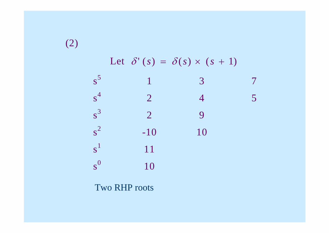
(2)

Let δ δ' ( ) ( ) ( )s s s= × + 1

s5 1 3 7

s4 2 4 5

s3 2 9

s2 -10 10

s1 11

s0 10

Two RHP roots

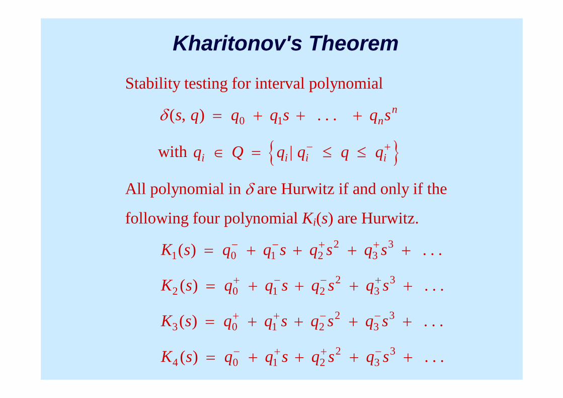
Kharitonov's Theorem

Stability testing for interval polynomial

δ ( , ) . . .s q q q s q snn= + + +0 1

with { }q Q q q q qi i i i∈ = ≤ ≤− +|

All polynomial in δ are Hurwitz if and only if the

following four polynomial Ki(s) are Hurwitz.

K s q q s q s q s1 0 1 22

33( ) = + + + +− − + + . . .

K s q q s q s q s2 0 1 22

33( ) = + + + ++ − − + . . .

K s q q s q s q s3 0 1 22

33( ) = + + + ++ + − − . . .

K s q q s q s q s4 0 1 22

33( ) = + + + +− + + − . . .

Lyapunov FunctionA scalar function V(x, t) is called a Lyapunov function if for all

t t≥ 0 and all vectors x in the neighbourhood of the origin, it satisfies

the following conditions.

1. V(0, t) = 0

2. V x t V x tt

V x tx

i ni

( , ), ( , ) ( , ) , , . . . ,∂∂

∂∂

and

= 1 , all exist and

are continuous.

3. V x t x( , ) ( )> >α 0 , for all x ≠ 0 and t t≥ 0 , where α( )⋅ isa non-decreasing function of x and α( )0 0= , that is, V(x, t) is

bounded below by a non-zero function.

Lyapunov Stability Analysis

Theorem: (Sufficient condition)

The equilibrium state xe = 0, of the system&( ) ( , ), ( , )x t f x t f t= =0 0 is asymptotically stable if a Lyapunov

function V(x, t) can be found such that &( , )V x t < 0 for all x ≠ 0and t t≥ 0

Theorem: (Sufficient condition)

The equilibrium state xe = 0, of the system&( ) ( , ), ( , )x t f x t f t= =0 0 is unstable if a Lyapunov

function V(x, t) can be found such that &( , )V x t > 0 for allx ≠ 0 and t t≥ 0

Example

& ( )xt

x t= −+

−⎛

⎝⎜⎜

⎞

⎠⎟⎟

0 11

315 . Determine the stability of the above

system choosing V x t x t x( , ) [ ( ) ]= + +12

312

22 .

Solution:

& ( , ) ( , )&V x t V x t

tVx

xii

n

i= +=

∑∂∂

∂∂ 1

0)8930(

21

)3(21

22

221122

<+−=

+++=

xt

xxtxxx &&

This indicates that the origin is asymptotically stable.

The linear system &( ) ( ) ( )x t A t x t= where A(t) is continuous

and bounded for t t≥ 0 , is uniformly asymptotically stable,

iff given a positive definite real matrix Q(t), there exists a

symmetric positive definite real matrix P(t)

which satisfies

&( ) ( ) ( ) ( ) ( ) ( ),P t A t P t P t A t Q t t tT+ + = − ≥ 0

Stability Theorem

Proof of TheoremLet V x t x t P t x tT( , ) ( ) ( ) ( )= .

)t(x)t(P)t(x)t(x)t(P)t(x)t(x)t(P)t(x)t,x(V TTT &&&& ++=

= + +

= −

x t A t P t P t A t P t x t

x t Q t x t

T T

T

( )( ( ) ( ) ( ) ( ) &( )) ( )

( ) ( ) ( )

&( , )V x t is a negative definite quadratic form and the system

is asymptotically stable.

Note: For linear time invariant system &( ) ( )x t Ax t= ,

the corresponding equation to be used is

A P PA QT + + = 0

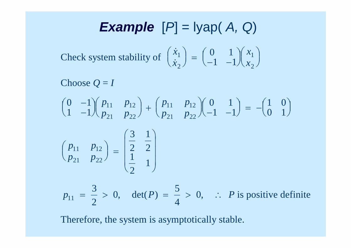
Example [P] = lyap( A, Q)

Check system stability of &&xx

xx

1

2

1

2

0 11 1

⎛⎝⎜

⎞⎠⎟

= − −⎛⎝⎜

⎞⎠⎟⎛⎝⎜

⎞⎠⎟

Choose Q = I

0 11 1

0 11 1

1 00 1

11 12

21 22

11 12

21 22

−−

⎛⎝⎜

⎞⎠⎟⎛⎝⎜

⎞⎠⎟

+ ⎛⎝⎜

⎞⎠⎟ − −⎛⎝⎜

⎞⎠⎟ = −⎛

⎝⎜⎞⎠⎟

p pp p

p pp p

p pp p

11 12

21 22

32

12

12

1

⎛⎝⎜

⎞⎠⎟ =

⎛

⎝

⎜⎜⎜

⎞

⎠

⎟⎟⎟

p P P1132

0 54

0= > = > ∴, det( ) , is positive definite

Therefore, the system is asymptotically stable.