Stability Analysis of the Earth Dams

and Dikes under the Influence of

Precipitation and Vegetation

DISSERTATION

to obtain the academic degree

Doctor of Engineering

(Dr.-Ing.)

Faculty of Environmental Sciences

Technische Universität Dresden

By

M.Sc. Jinxing Guo

Matriculation Number: 3638372

Born on Oct. 14, 1985 in Jiangsu, China

Supervised by

Prof. Dr. Peter-Wolfgang Graeber

Prof. Dr. Rudolf Liedl

Prof. Dr. Peter Werner

Table of Contents

Abstract ……………………………………………………………………………………………………………………………….i

Acknowledgements……………………………………………………………………………………………………………….ii

List of Symbols and Abbreviations………………..…………………………………………………………………….. iii List of Figures……………………………..………………………………………………………………………………………v List of Tables…………………………………………………………………………………………………………………….…...x

CHAPTER 1 Introduction……………………………………………………………………………………….………………1

CHAPTER 2 Problems and Objectives……………………………………………………………………………………3

CHAPTER 3 Basics Knowledge……………………………………………………………………………………………….4

3.1 Description of the earth dam and dike structure……………………………………………………….4

3.2 Hydrological process in the dam and dike body………………………………………………………..5

3.2.1 Seepage flow………………………………………………………………………………………………………5

3.2.2 Capillary rise……………………………………………………………………………………………………….7

3.3 Factors affecting the hydrological process……………………………………………………………….8

3.4 Stability problem in the earth dam and dike………………………………………………………….11

3.4.1 Causes of slope landslides………………………………………………………………………………..11

3.4.2 Types of slope landslides………………………………………………………………………………….13

CHAPTER 4 Methodology for Hydrological Process Simulation…………………………………………15

4.1 General description of the Program PCSiWaPro®……………………………………………………..15

4.2 Theoretical Background of the Program PCSiWaPro®……………………………………………….15

4.3 Advantage of the Program PCSiWaPro®……………………………………………………………………16

4.4 Model Setup of an earth dam in PCSiWaPro®……………………………………………………………18

CHAPTER 5 Methodologies for Stability Analysis……………………………………………….………………20

5.1 Factor of safety (Fs)…………………………………………………………………………………………………..20

5.2 The basic Mohr- Coulomb Model………………………………………………………………………….…..20

5.2.1 Theoretical background…………………………………………………………………………………….21

5.2.2 Cohesion (c’) change related to soil water content…………………………………………….22

5.2.3 Matric suction (Ua – Uw) change due to water content change………………………….26

5.2.4 Internal friction change due to the water content change……………………28

5.2.5 change due to the water content change……………………………………………….30

5.3 Influence of vegetation on the slope stability……………………………………………………………31

5.3.1 Hydrological effects of vegetation……………………………………………………………………..31

5.3.2 Root reinforcement cohesion…………………………………………………………………………….32

5.4 The Infinite Slope Model for the surficial landslides………………………………………………….33

5.5 The BISHOP’S Model for the deep landslides……………………………..……………………………35

5.6 Application of the GEO-SLOPE Program……………………………………………………………………37

5.6.1 Description of the GEO- SLOPE Program……………………………………………………………37

5.6.2 Disadvantage of the GEO- SLOPE Program…………………………………………………………41

CHAPTER 6 Discussion on Simulation Results of PCSiWaPro®………………………………………….…43

6.1 Simulation for a physical dam……………………………………………………………………………………43

6.1.1 General description of the physical dam……………………………………………………………43

6.1.2 Simulation results………………………………………………………………………………………………43

6.1.3 Sensitivity analysis of model parameters…………………………………………………………..46

6.2 Simulation for a Chinese earth dam………………………………………………………………………….48

6.2.1 Site description………………………………………………………………………………….………………48

6.2.2 Hydrological simulation results………………………………………………………….………………49

6.2.3 Comparison between the measured and simulated results………………….……………55

6.3 Simulation for a dump slope of the mining pit……………………………………………….………….57

6.3.1 Site description…………………………………………………………………………………………………57

6.3.2 Hydrological simulation results…………………………………………………………………………58

6.3.3 Comparison between the measured and simulated results.................................61

6.4 Conclusion…………………………………………………………………………………………………………………62

CHAPTER 7 Discussion on stability analysis results……………………………………………………………64

7.1 Infinite slope analysis for the surficial landslide………………………………………………………..64

7.1.1 Infinite slope analysis for the Chinese earth dam………………………………………………64

7.1.2 Infinite slope analysis for the dump slope………………………………………………….………71

7.1.3 Conclusions……………………………………………………………………………………………………….75

7.2 BISHOP’S Model analysis for the circle and deep landslide…………………….……………..…76

7.2.1 BISHOP’S Model analysis for the Chinese earth dam…………………………….……………76

7.2.1.1 Stability analysis by the GEO-SLOPE Software………………………………………….76

7.2.1.2 Sensitivity analysis of the soil parameters in the GEO-SLOPE …………………..80

7.2.1.3 Improvement of the stability analysis results……………………………………………83

7.2.2 BISHOP’S Model analysis for the dump slope…………………………………………………….87

7.2.2.1 Stability analysis in the GEO-SLOPE Software…………………………………………..87

7.2.2.2 Improvement of the stability analysis results……………………………………………91

7.3 Conclusions……………………………………………………………………………………………………………….94

CHAPTER 8 Conclusions and recommendation…………………………………………………………………..97

8.1 Conclusions……………………………………………………………………………………………………………….97

8.2 Recommendations and future research work…………………………………………………………100

References ………………………………………………………………………………………………………………………101

Appendix...............................................................................................................................111

Declaration

I declare that I have finished the present work independently without outside help and I

have made no use other than the specified sources.

Date Signature

i

Abstract

An earth dam and a dike is one kind of hydraulic construction, which is built with highly

compacted earth and can be used for the purpose of containing water in a reservoir to

secure the water supply, and in flood control. Earth dam and dike can be a safety issue, as it

can experience catastrophic destruction due to the slope failure caused by various factors,

such as construction materials, vegetation, atmospheric conditions and so on. The aim of

this study is to investigate the influence of the saturation degree (or water content) on the

stability of earth dam and dikes under the consideration of precipitation and vegetation with

the program PCSiWaPro® (developed at the Technical University of Dresden, Institute of

Waste Management and Contaminated Site Treatment).

The preliminary tests on a physical model have shown that the security and stability has

been already severely compromised in the partially saturated region, i.e. the area above the

seepage line was in great danger and it came quickly to landslides on the air side. Before the

stability analysis could be done for those unsaturated zones, water flow processes and water

saturation in the saturated and partially saturated soil area were simulated using the

simulation program PCSiWaPro® under transient boundary conditions (Graeber et al. 2006).

The integration of a weather generator into PCSiWaPro® allows a transient water flow

calculation with respect to atmospheric conditions (precipitation, evaporation, daily mean

temperature and sunshine duration) and removal of water by plant roots and leaves. Finally,

with the Program PCSiWaPro® and Gmsh, a 2D dynamic model of water content distribution

in the earth dam could be built, incorporating information of not only climate parameters

and vegetation but also geometry, soil properties, geohydraulic conditions and time-

dependent boundary conditions. The simulation results of several scenarios both in the

laboratory and in the field of China and Germany clearly demonstrated that the accordance

between measured values and calculated values for water content using the simulation

program PCSiWaPro® was very good.

In addition, two kinds of stability analysis models (the Infinite Slope Model and the BISHOP’S

Model, one kind of the limit equilibrium method), which were both developed from the old

Mohr-Coulomb Model, have been improved with the additional consideration of root

reinforcement in the upper layer of the slope and soil water in the earth slope. The Infinite

Slope Model has been proved to be mainly applied for the surficial landslide; while the

BISHOP’S Model is more responsible for the deeper slip landslide forecasting. Then based on

the PCSiWaPro® simulation result of water content in the unsaturated slope in the earth

bodies from two study sites, Fs (safety of factor) calculation for those earth slopes was

derived providing a sufficient forecasting system for the slope-failure-flood. The results have

been compared with the calculated Fs values from the old models (without consideration of

the influence of water content change on the slope stability) to study how significantly water

content increased the risk of slope landslides.

ii

Acknowledgements

This work has been performed during the period from the winter semester of 2011/12 to the

winter semester of 2014/15 in the Institute of Waste Management and Contaminate Site

Treatment at the Department of Hydro Sciences at the Technical University of Dresden.

I wish to express my sincere appreciates to my dear principal supervisor Prof. Dr.- Ing. habil

Peter- Wolfgang Graeber for his greatly important technical guidance, financial support and

professional advice during my research work, which is always beneficial interest and

valuable on the implementation and evaluation of my research. In addition, together with

him, I have learnt a lot not only about the study but also for the life experience; my PhD

study here could be among the most valuable times in my life. Special thanks are given to

Prof. Dr. Rudolf Liedl for his valuable scientific remarks and significant correction in my thesis

from which I have learnt a lot about how to better write a scientific thesis. Special thanks are

also given to my former colleague Dr. Issa Hasan for his guidance of the application of the

Program PCSiWaPro® and technical support in the beginning of my research. Special thanks

are given to Dr. Catalin Stefan with whom I have had lots of interesting discussion and

carried out lots of research work in the Project INOWAS and sincere appreciate to his

financial support. In addition, I also want to express my sincere thanks to the Graduate

Academy at the Technical University of Dresden for their four-month financial support on my

research.

Sincere thanks to the master student for her data collection in China; and special thanks are

also extended to Dr. Axel Fischer, Mrs. Jutta Sitte and Mrs. Claudia Schoenekerl for their

friendly support in my life in the institute, and to all the other members of the System

Analysis Group with whom I have had a nice life during my working in Pirna.

Last but certainly not least, great thanks to my wife and my whole family who have held me

up when I could not stand up. You have been the best personal cheering squad anyone could

ask for.

iii

List of Symbols and Abbreviations

mean root cross-sectional area of a root diameter class

A reference area, vertical projection of the above-ground biomass of the plant

Ar root area

width of the ith slice

soil cohesion

c‘ the soil cohesion at water content θ

cohesion of the ith slice, depending on the saturation

c0 soil cohesion with the residual soil water content of θr

cohesion due to roots

cS soil cohesion with full water saturation θS

Fc the cohesion force

Fc(s) the constant cohesion force in the soil

Fs factor of safety

g the acceleration due to gravity

normal stress due to gravity

- net normal stress

h pressure head

hc the pressure head difference between the wetting (water) and non-wetting phase (air)

height of the unsaturated part above the seepage line in the ith slice

total height of the ith slice

the permeability of the soil medium

K the hydraulic conductivity

n slope factor, the empirical VAN-GENUCHTEN parameter

the number of long roots in each root diameter class

q the Darcy velocity

the length of that air-water interface in the jth pore space acting to pull the particles together

S source/sink term

shear stress for the balance required

Se the saturation degree

RAR root area ratio

t time

rate of increase in shear strength relative to matric suction

iv

the pore air pressure

V flow discharge per unit area

µ the water viscosity

pore pressure in the ith slice, depending on the saturation

saturated pore water pressure under the seepage line

- matric suction

the pore water pressure

total soil-water weight of the ith slice

Z the vertical depth below the ground surface

α scale factor, the empirical VAN-GENUCHTEN parameter

the angle between the shear force on the ith slice and horizontal face

β the slope angle of the earth structure

γ the total soil and water unit weight

γsoil soil unit weight

water content in the soil

r residual water content

r,l residual air content

saturated water content

ρ the fluid density

σ the normal stress

tensile strength of the root material

σs the suction stress characteristic curve of the soil with a practical functional form

σt the surface tension of the air-water interface

total shear strength inside the soil

shear stress on the failure plane at failure

φP the porosity of the soil

the angle of internal friction in the soil

internal friction angle of the ith slice, depending on the saturation

r soil internal friction angle with the residual water content of θ

s soil internal friction angle with the saturated water content of θ

∇h the hydraulic gradient

v

List of Figures

Figure 1.1 Water balance in the saturated and partially saturated region……………………..2

Figure 3.1 An example of homogeneous earthfill dam profile……………………………………….4

Figure 3.2 Types of earth dams with different structures, e.g. impermeable cores……….5

Figure 3.3 Seepage line in a small earth dam………………………………………………………………..6

Figure 3.4 Schematic representation of capillary region in an earth dam……………………...7

Figure 3.5 Comparison of the seepage line position in a homogeneous earth dam with three structures………………………………………………………………………………………….10

Figure 3.6 Diagram illustrating the resistance to, and causes of, movement in a slope system consisting of an unstable block……………………………………………………….11

Figure 3.7 Process of backward erosion………………………………………………………………………13

Figure 3.8 An idealized slump-earth flow showing commonly used nomenclature for labeling the parts of a landslide………………………………………………………………….13

Figure 3.9 Potential Slope Stability Failures…………………………………………………………………14

Figure 4.1 Operation interface of parameter estimation using pedotransfer function in PCSiWaPro® ……………………………………………………………………………………………….16

Figure 4.2 Operation interfaces of the weather generator for an example in the Dresden area…………………………………………………………………………………………………………….17

Figure 4.3 An example of the input system interface of the measured pressure head data for the observation point (470, 15.2)………………………………………………….18

Figure 4.4 Setup of various boundary conditions in the program PCSiWaPro® ……………18

Figure 4.5 Input of the soil parameters into the program PCSiWaPro………………………….19

Figure 5.1 Graphic expression of Mohr-Coulomb Model (A is for the cohesionless soil like gravel sand, and B is for the cohesive soil like clay soil)………………………..21

Figure 5.2 Idealized particles held together by water………………………………………………….23

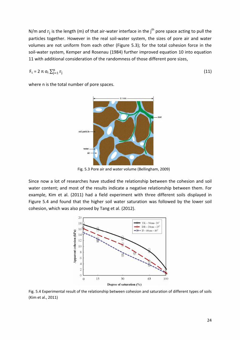
Figure 5.3 Pore air and water volume………………………………………………………………………….24

Figure 5.4

Experimental result of the relationship between cohesion and saturation of different types of soils………………………………………………………………………………..24

Figure 5.7 Relationship between matric suction and water content for different soils…………………………………………………………………………………………………………….27

Figure 5.8 Effect of matric suction on factor of safety in a residual granite soil slope….28

Figure 5.9 Experimental results of the correlation between internal friction and saturation for three types of soils……………………………………………………………….28

Figure 5.10 the relation curve between the internal friction angle and water saturation……………………………………………………………………………………………………29

Figure 5.11 Variation of shear strength with respect to matric suction…………………………30

vi

Figure 5.12 Plant reinforcement in riprap and small fills……………………………………………….32

Figure 5.13 Slope cross-section for infinite slope equation……………………………………………34

Figure 5.14 Method of slices of BISHOP’S Model for the circular type of sliding surface………………………………............................................................................36

Figure 5.15 Force analysis of one typical slice for BISHOPS Model ..................................36

Figure 5.16 Grid and radius option used to determine the critical slip circular in GEO-SLOPE ……………………………………………………………………………………………………………38

Figure 5.17 Input of groundwater table into the GEO-SLOPE Program………………………….39

Figure 5.18 Summary of all the calculated factors of safety and the contour of the critical slip surface………………………………………………………………………………………………….39

Figure 5.19 Division of the slope above the critical slip surface……………………………………..40

Figure 5.20 An example for the free body diagram and force polygon analysis with the BISHOP’S Model………………………………………………………………………………………….40

Figure 5.21 Input of material property values (cohesion and internal friction angle) in the Geo-SLOPE…………………………………………………………………………………….………………41

Figure 5.22 An earth slope body being passed through by the seepage line (the blue line is the seepage line)……………………………………………………………………………………........42

Figure 6.1 A physical model dam with slides on the air side…………………………………........43

Figure 6.2 Water saturation simulation by PCSiWaPro® with increasing the water level in the left side of dam…………………………………………………………………………………44

Figure 6.3 Pressure head simulation by PCSiWaPro® with increasing the water level in the left side of dam……………………………………………………………………………………44

Figure 6.4 Daily precipitation data of Dresden from the weather generator of PCSiWaPro®………………………………………………………………………………………………..45

Figure 6.5 Water saturation distribution simulated by PCSiWaPro® in a physical earth dam without input of rainfall water…………………………………………………………….45

Figure 6.6 Water content distribution simulated by PCSiWaPro® in a physical earth dam in a heavy rainfall event………………………………………………………………………………46

Figure 6.7 Pressure head distribution simulated by PCSiWaPro® in a physical earth dam in a heavy rainfall event………………………………………………………………………………46

Figure 6.8 Water saturation distribution simulated by PCSiWaPro® in a physical earth dam with the Van Genuchten Parameters α = 1 m-1, n = 1.9……………………….47

Figure 6.9 Water saturation distribution simulated by PCSiWaPro® in a physical earth dam with the Van Genuchten Parameters α = 2 m-1, n = 1.9……………………….47

Figure 6.10 Setup of soil materials in the Chinese earth dam in PCSiWaPro® ……………….48

Figure 6.11 Precipitation and water level changes during the simulation period of 9 months in the reservoir………………………………………………………………………………49

Figure 6.12 Setup of boundary conditions for this Chinese earth dam…………………………..49

vii

Figure 6.13 Pressure head simulation from PCSiWaPro® on 29.06.2012……………………….50

Figure 6.14 Water content simulation from PCSiWaPro® on 29.06.2012……………………….51

Figure 6.15 Water saturation simulation from PCSiWaPro® on 29.06.2012……………………52

Figure 6.16

Water content simulation from PCSiWaPro® on 20.06.2012 with a wet weather………………………………………………………………………………………………………53

Figure 6.17 Water saturation simulation from PCSiWaPro® on 20.06.2012 with a wet weather……………………………………………………………………………………………………...53

Figure 6.18 Water content distribution in the unsaturated slope during the wet and dry weather………………………………………………………………………………………………………54

Figure 6.19 Position of the two observation points in the Chinese earth dam.................55

Figure 6.20 Comparison between the computed and measured water levels in an observation point in the clay core……………………………………………………………….56

Figure 6.21 Comparison between the computed and measured water levels in an observation point in the slope…………………………………………………………………….56

Figure 6.22 A simplified structure of a dump site…………………………………………………………..57

Figure 6.23 Location of this study area………………………………………………………………………….57

Figure 6.24 Structure of this dump slope generated by PCSiWaPro® with clay soil and different sandy soils……………………………………………………………………………………58

Figure 6.25 Water saturation simulation without input of precipitation on July 30th, 2003 (the white lines represent the borders of different soil layers)……………………59

Figure 6.26 Water content simulation results without input of precipitation on July 30th, 2003…………………………………………………………………………………………………………...60

Figure 6.27 Typical precipitation data for one year in Leipzig from the weather generator in PCSiWaPro®…………………………………………………………………………………………….60

Figure 6.28 Simulation of water saturation distribution with input of precipitation on April 30th, 2003……………………………………………………………………………………………61

Figure 6.29 Simulation of water saturation distribution with input of precipitation on July 30th, 2003……………………………………………………………………………………………………61

Figure 6.30 Simulation of water saturation distribution with input of precipitation on August 20th, 2003………………………………………………………………………………………..62

Figure 6.31 Comparison between the simulation data and the measurement data in the observation well……………………………………………………………………………………………62

Figure 7.1

Water content distribution simulated by PCSiWaPro® in the Chinese earth dam on 29.06.2012 during a dry weather……………………………………………………64

Figure 7.2 One part of the unsaturated slope with water content simulation result from PCSiWaPro® during a dry weather on 29.06.2012……………………………………….65

Figure 7.3 One part of the unsaturated slope with water content simulation result from PCSiWaPro® during a wet weather (20.06.2012)…………………………………………68

viii

Figure 7.4 Simulation of water saturation in the dump slope on a dry weather on 30th April, 2003…………………………………………………………………………………………………..71

Figure 7.5 A selected part from the unsaturated sandy slope for the stability analysis……………………………………………………………………………………………………….71

Figure 7.6 Simulation of water saturation in the dump slope on a wet weather on 30th July, 2003……………………………………………………………………………………………………73

Figure 7.7 A selected part from the unsaturated sandy slope for the stability analysis............................................................................................................74

Figure 7.8 Simulation result of water content in the Chinese earth dam on 29.06.2012………………………………………………………………………………………………….76

Figure 7.9 Setup of grid (50*50) and tangent lines (20) to determine the different radius of circular slipe surface in the earth dam slope with the software Geo-slope……………………………………………………………………………………………………………77

Figure 7.10 Critical slip surface analysis by the GEO-SLOPE depending on the simulation result of the seepage line position from the program PCSiWaPro® …............77

Figure 7.11 Distribution map of Fs values for this Chinese earth dam with the minimum value in the middle……………………………………………………………………………………..78

Figure 7.12 Division of the slope above the critical slip surface into total 31 slices by the GEO-SLOPE …………………………………………………………………………………………………79

Figure 7.13 Force analysis for the 4th slice above the seepage line………………………………..80

Figure 7.14 Force analysis for the 20th slice under the seepage line………………………………80

Figure 7.15 Sensitivity analysis of the soil cohesion in the GEO-SLOPE Software……………..81

Figure 7.16 Sensitivity analysis of the internal friction angle with a fixed cohesion in the GEO-SLOPE Software…………………………………………………………………………………….82

Figure 7.17 Critical slip surface with the water content simulation result for 29.06.2012………………………………………………………………………………………………….83

Figure 7.18 Division of the unsaturated slope into 31 slices with the water content simulation result…………………………………………………………………………………………84

Figure 7.19 Stability analysis by the GEO-SLOPE with the input of the saturated soil parameters………………………………………………………………………………………………….85

Figure 7.20 Division of the critical slip surface into total 35 slices………………………………….86

Figure 7.21 Input of the influence of soil water into this earth slope…………………………....86

Figure 7.22 Definition of the possible position of the critical slip surface (area between the two white borders)……………………………………………………………………………….87

Figure 7.23 Simulation of water saturation distribution with input of precipitation on July 30th, 2003……………………………………………………………………………………………………88

Figure 7.24 Setup of grids and tangent lines in the dump slope within the Software GEO-SLOPE …………………………………………………………………………………………………………..88

Figure 7.25 Critical slip surface analysis for the sandy dump slope by the Geo-slope depending on the simulation result of the seepage line position from the program PCSiWaPro® …………………………………………………………………………………89

ix

Figure 7.26 Distribution map of the Fs values in the dump slope…………………………………..89

Figure 7.27 Division of the slope above the critical slip surface into total 30 slices calculated from the Software GEO-SLOPE ……………………………………………….....90

Figure 7.28 Force analysis for the No.4 slice above the groundwater table……………………90

Figure 7.29 Force analysis for the No.18 slice which is passed through by the groundwater t a b l e … … … … … … … … … … … … … … … … … … … … … … … … … … … … … … … … … 9 0

Figure 7.30 Analysis of slices above the critical slip with the consideration of soil water in the dump slope…………………………………………………………………………………………..91

Figure 7.31 Position of the critical slip surface and the distribution of the Fs values from the GEO-SLOPE Software………………………………………………………………………………92

Figure 7.32 Analysis of all those 31 slices above the critical slip surface………………………..93

Figure 7.33 Analysis of slices above the critical slip with the consideration of soil water in the dump slope…………………………………………………………………………………………..93

Figure 7.34 Possible position area of the critical slip surface…………………………………………94

Figure 8.1 Process of the improved stability analysis in the study……………………………….99

x

List of Tables

Table 1 Typical values of customary safety factors, Fs…………………………………………20

Table 2 Comparison of water content in the different layers during the wet and weather…………………………………………………………………………………………………..55

Table 3 Fs results from the infinite slope model…………………………………………………..66

Table 4 Fs values with the improved soil parameter values due to the water content change……………………………………………………………………………………….67

Table 5 Fs results from the original infinite slope model and the improved Model A……………………………………………………………………………………………………………..69

Table 6 Fs values from the Model B (with improved soil parameters’ values)………70

Table 7 Fs results from the original infinite slope model and improved Model A…72

Table 8 Fs values from the improved Model B (with improved soil parameter values)…………………………………………………………………………………………………….73

Table 9 Calculation of the improved BISHOP’S Model for the Chinese dam slope..74

Table 10 Calculation of the improved BISHOP’S Model for the Chinese dam slope..75

Table 11 Sensitivity analysis of the soil cohesion in the GEO-SLOPE Software with the fixed Ф'…………………………………………………………………………………………….82

Table 12 Sensitivity analysis of the internal friction angle in the GEO-SLOPE Software with the fixed c'……………………………………………………………………………………….83

Table 13 Improved values of cohesion and internal friction angle for the dump sand…………………………………………………………………………………………………………91

Table 14 Improved values of cohesion and internal friction angle…………………………93

Table 15 Comparison of the stability analysis results with the infinite slope analysis model……………………………………………………………………………………………………..96

Table 16 Comparison of the stability analysis results with the BISHOP’S Model…….96

1

Chapter 1 Introduction

River regions were always the first cradles of human history. Water plays a crucial role for

domestic use and agriculture. Therefore, many cities are close to or even built directly on the

banks of a river. However at the same time we are always warned to think about the risk of

flooding there. An earth dam and a dike is one kind of hydraulic construction structure built

with highly compacted earth and used for the purpose of flood control (Bassell, 1904).

Worldwide there are millions of kilometers of dam and dike length, and only in the State of

Lower Saxony in Germany there are around 645 km of dike length (Schuettrumpf, 2008).

However, severe flood events occur every year due to dam collapse, for example, the flood

caused by the Elbe River in 2002 (SMUL, 2007) and in Fischbeck in July 2013 (Jonkman et al.,

2013).

Surface erosion (surface overflow) and increase of water saturation in the dam body are the

main causes of dam instability risk (Bonelli, 2013). There was an early assumption that the

landslides and suffosion phenomenon can arise only in the fully saturated soil areas on the

air side; however Aigner (2004) showed by physical experiments that this could occur even

in the partially saturated soil area of the dam. The surface erosion is relatively easy to be

detected and avoided, while the soil moisture increase risk cannot be easily identified.

Therefore, these hydraulic structures are more dangerous due to the rise and the flow from

the ground water in the unsaturated zones (Bonelli, 2013).

In those unsaturated areas, various factors can influence the water balance and then the

stability, for example, construction methods, soil materials, geometry, atmospheric

conditions (e.g. precipitation), and even vegetation (Wu, 2013) (see Fig. 1.1). Precipitation

can increase the water level in the reservoir and river which then drives the rising movement

of seepage line in the dam and dike body. In addition, the precipitation has also direct

influence on the water content change with the infiltration water in the unsaturated slope

and then changes the seepage line movement regime (especially in an extreme rainfall

event). The significant influence of vegetation on slope stability can essentially be attributed

to two major aspects: water movement via the soil–plant–atmosphere continuum (SPAC)

(Coppin et al., 1990) and soil reinforcement by the root system (Gray, 1995). Vegetation is a

major component of SPAC, responsible for the suction force of water against gravity. By

absorbing parts of the soil water, plants thus play a significant role in the drying of slopes

(Huang and Nobel, 1994). This absorbed soil water will subsequently be removed through

the transpiration process into the atmosphere (Coppin et al., 1990). Ultimately, this water

cycle system would result in less saturated and more stable slopes. Concurrently, vegetation

also contributes to mass stability by increasing the soil shear strength through root

reinforcement (Gray, 1995). The frequency of slope failures tends to increase when

vegetation is cut down and their roots decay (Abe, 1997).

2

Fig. 1.1 Water balance in the saturated and partially saturated regions of an earth dam (Hasan et al., 2012)

Since now lots of researches about the stability analysis of dam and dike slopes have been

carried out; and several applicable methodologies have been put forward, like the infinite

slope analysis model and the limit equilibrium models (Bishop’s Model, Ordinary method of

slices, Spencer Method…) which are based on the typical Mohr-Coulomb Model to express

the safety factor in the earth slopes. Both of those models have their own advantages and

disadvantages; for example, the infinite slope model is more suitable and convenient for the

surficial slope stability analysis especially in the quick decision support system for the risk

assessment work but with low accuracy for the deep slope landslide forecasting; while the

limit equilibrium models are professional for the circular slip surface analysis in the deep

slope and could provide a much higher accuracy but with much more complicated

calculation process.

3

Chapter 2 Problems and Objective

Since now there are various kinds of stability analysis methodologies and software having

been developed. However the improvement of the accuracy of those methodologies and

technologies is still a popular and open issue; for example, in the common stability analysis

work, the factors of water content and vegetation on the stability assessment for the

unsaturated earth slopes have been always neglected or roughly estimated, which could

result in the overestimation or great roughness for the slope-failure forecasting especially

during the heavy rainfall events.

In order to overcome this disadvantage, this study mainly focuses on the investigation of the

hydrological regime in unsaturated earth slopes and the study of the influence from water

content and vegetation on the slope stability depending on the improved stability analysis

models (infinite slope analysis model and Bishop’s Model).

Generally, this study has different kinds of aims shown below:

To study the hydrological regime in the earth slopes under different boundary

conditions, e.g. investigation of the influence of precipitation on the hydrological regime

in the earth dam and dike slopes;

to put forward a new method for scenario analysis and prediction of the stability of

earth dams and dikes, especially in the flood period and during the heavy rainfall event,

which can help to prevent or at least reduce the great damage as a result of earth slope

failures;

additional consideration of water content in the unsaturated slope and the effects from

vegetation on the slope stability in order to improve the slope-failure forecasting

accuracy;

comparison of the stability analysis results from the infinite slope model and the

Bishop’s Model in the study sites;

analysis and optimization of hydraulic protective building systems to support the

management, planning and development of these systems;

improvement of the perception and understanding of the risk of the structures of earth

dams and dikes;

to prevent material and human losses and lead to an effective disaster management

before and during the flood;

"know-how" - transfer to other European and non-European countries.

4

Chapter 3 Basic Knowledge

3.1 Description of the hydraulic structure

Dams, which are intended to store large volumes of water, must necessarily be built of

considerable height (Bassell, 1904). Dams may be classified into diverting dams or weirs and

storage dams. The former may be located upon any portion of a stream where the

conditions are favorable for construction, and the water is suitable for domestic, agriculture

and industry purposes, being conveyed by structures of canals, flumes, tunnels and pipe

lines to places of intended use. Storage dams can be divided into several groups: (1) earth; (2)

earth and timer; (3) earth and rock-fill; (4) rock-fill; (5) masonry; (6) composite structures

(Bassell, 1904).

An earthfill dam is made up partly or entirely of pervious material which consists of fine

particles, usually clay, or a mixture of clay and silt or a mixture of clay, silt and gravel. They

are principally constructed from available excavation material. The dam is built up with

rather flat slopes. Fine, impervious material of an earthfill dam occupies a relatively small

part of the structure, it is known as the core. The core is located either in a central position

or in a sloping position upstream of the center. If the remaining materials consist of coarse

particles, there is a gradation in fineness from the core to the coarse outer materials. Some

earth dams have a large proportion of rock in the outer zones for the purpose of stability

(Ersayin, 2006).

Most new earthfill dams can be further classified as homogenous, zoned, or diaphragm (U.S.

Bureau of Reclamation, 1987). Homogenous earthfill dams are composed of only one kind of

material (Fig. 3.1), besides the slope protection material. The material used must be

impervious enough to provide an adequate water barrier and the slope must be relatively

flat for stability. It is more common today to build modified homogeneous earth dams in

which impermeable cores are placed to control steeper slopes and get more stability shown

in Fig. 3.2 (Ersayin, 2006; U.S.A.C.E, 2004).

Fig. 3.1 An example of homogeneous earth dam profile (Giglou and Zeraatparvar, 2012)

5

Fig. 3.2 Types of earth dams with different structures, e.g. impermeable cores (U.S.A.C.E., 2004)

Similar to the earth dam, the dike is also one kind of earth embankment which is commonly

built along the river channels and the coastal lines to prevent the possible flood damage. The

earth dike can be formed by the compacted soils and the slope of the dike is usually

stabilized by the vegetation (GA Ltd. and AE Ltd., 2003).

3.2 Hydrological processes in the dam and dike body

3.2.1 Seepage flow

Water flow through the dam is one of the basic problems for geotechnical engineers.

Seepage is the continuous movement of water from the upstream face of the dam toward its

downstream face. The upper surface of this stream of percolating water is known as the

6

phreatic surface (Moayed et al., 2012). In two dimension the seepage line (Fig. 3.3) refers to

a line of atmospheric pressure (that is, the pressure head is zero) and is the border of the

saturated and unsaturated zones (Ersayin, 2006).

Fig. 3.3 Seepage line in a small earth dam (Nelson, 1985)

The seepage can be found in all earth dams as the impounded water seeks the paths with

the least resistance to its flow and passes through the dam and the foundation. Seepage can

be detected anywhere on the downstream face of the dam, beyond the toe, or on the

downstream abutments at elevations below normal water level. The seepage may exhibit in

some critical forms like a "soft" wet area and a flowing "spring." A continuous or sudden

drop in the normal lake level is one indication that considerable seepage will happen. In this

case, one or more locations of flowing water are usually concentrated to flow downstream

from the dam. If the seepage forces are large enough, soil in the dam body can be eroded

from the foundation and then be deposited into the cone shape around the outlet, which is

called the boils phenomenon. If these "boils" appear, professional advice should be sought

immediately. Seepage flow with mud and sediment (soil particles) is evidence of "piping"

which can most often occur along a spillway or other conduit through the embankment.

Sinkholes may be developed on the surface of the embankment after internal erosion taking

place. This may be followed by a whirlpool in the lake surface and then likely a rapid and

complete failure of the dam (NYSDEC, 1987).

Seepage becomes a concern, as portions of the embankment and foundation can be

saturated and weakened, which makes the embankment and foundation susceptible to

earth slides; and it can also carry soil material resulting in erosion of the embankment and

foundation. In this case, it is extremely important to control the seepage and prevent the

seepage flow from removing soil particles. Modern design practice incorporates this control

into the dam design through the use of cutoffs, internal filters, and adequate drainage

provisions. Control at points where seepage exits can be realized after construction by

installation of toe drains, relief wells, or inverted filters (NYSDEC, 1987). In addition, regular

monitoring work is essential to detect seepage and prevent dam failure; based on the

knowledge on the dam's history data about the points of seepage exit, quantity and content

of flow, size of wet area, and type of vegetation, an easy comparison can help us to

7

determine whether the seepage condition is in a steady or changing state. Photographs

provide invaluable records of seepage. Instrumentation can also be applied to monitor the

seepage phenomenon (NYSDEC, 1987); for example, piezometers may be used to measure

the saturation level (phreatic surface) within the embankment whose data is the extremely

important basis for the future computer simulation and landslides forecasting work.

3.2.2 Capillary rise

Molecules within a liquid attract each other, and that attraction between molecules of the

same type is called cohesion. At the interface to the gas phase the resultant force is directed

downwards and the boundary surface acts as a tensile stress by stressed membrane (Thielen,

2007). This tensile stress effect is called surface tension which is the driving force of capillary.

Capillary water is held in the capillary pores (micro pores). Capillary water is retained on the

soil particles by surface tension forces. It is held so strongly that gravity cannot remove it

from the soil particles (USGS, 1988; Heath, 1983).

The capillary fringe is the subsurface layer in which ground water seeps up from a water

table by capillary action to fill pores (Fig. 3.4). Pores at the base of the capillary fringe are

filled with water due to tension saturation. This saturated portion of the capillary fringe is

less than total capillary rise because of the presence of a mix in pore size. If pore size is small

and relatively uniform, it is possible that soils can be completely saturated with water for

several feet above the ground water table. Alternately, the saturated portion will extend

only a few inches above the water table when pore size is large. Capillary action supports

a vadose zone above the saturated base within which water content decreases with distance

above the water table (USGS, 1988; Heath, 1983; U.S. EPA, 2009).

Fig. 3.4 Schematic representation of capillary region in an earth dam

The molecules of capillary water are free and mobile and are present in a liquid state. Due to

this reason, it evaporates easily at ordinary temperature though it is held firmly by the soil

particle; plant roots are able to absorb it. Capillary water is, therefore, known as available

water (USGS, 1988; Heath, 1983; U.S. EPA, 2009; AgriInfo.in, 2011).

8

3.3 Factors affecting the hydrological processes

Movement of groundwater in the earth dam depends on water level variation in the earth

dam (groundwater’s flow potential), soil properties (e.g. porosity and permeability),

hydraulic structures, atmospheric condition and vegetation.

Water level variation

Water level in the reservoir has a direct effect on the ground water table and then the

moving of the seepage line in the earth dam body. Water table contour lines are similar to

topographic lines on a map. They essentially represent "elevations" which are called the

hydraulic head denoted "h" in hydrology formulas. Changes in hydraulic head are the driving

force of groundwater flow. Groundwater always moves from an area of higher hydraulic

head to an area of lower hydraulic head. The ratio between the hydraulic head difference

and the distance of those two areas is called the hydraulic gradient. Groundwater not only

flows downward, it can also flow laterally or upward during the variation of water level in

the reservoir, i.e. there is a hydraulic gradient existing (Mulley, 2004; Chanson, 2004). The

rapid increase of water level always corresponds to the quick increase of hydraulic gradient

and then a quicker seepage flow which could further cause the instability of the earth slope.

Soil characteristics

In a certain soil the rate of groundwater flow is also controlled by soil properties, like

porosity and permeability (hydraulic conductivity).

Porosity is the percentage of the volume of the soil that is open space (pore space), and it

determines how much water one certain soil can contain. The porosity depends on the soil

grain size, the shapes of the grains, the degree of sorting and the degree of cementation

(Nelson, 2011). Poorly sorted soils usually exhibit lower porosity, which could be explained

by the fact that the fine-grained fragments are much easier to fill in the open space. Due to

the occupation of cements filled in the pore space, the cemented soils have lower porosity

than the normal soils (Nelson, 2011).

Permeability is a measure of the degree to which the pore spaces are interconnected, the

size of the interconnections and the ability of the soils to permit water to flow through its

pores (Nelson, 2011). High soil permeability can result in rapid water flow in the soil.

Porosity and permeability are two important components of hydraulic conductivity. The

definition of hydraulic conductivity (usually denoted ‘K’) is a property of soils describing the

ease with which water can move through pore spaces. It depends on the intrinsic

permeability of the soil material and on the degree of soil water saturation, and also on

the density and viscosity of the water fluid. Saturated soil hydraulic conductivity, Ksat,

describes water movement through saturated soil media (Darcy, 1856; Bear, 1972).

9

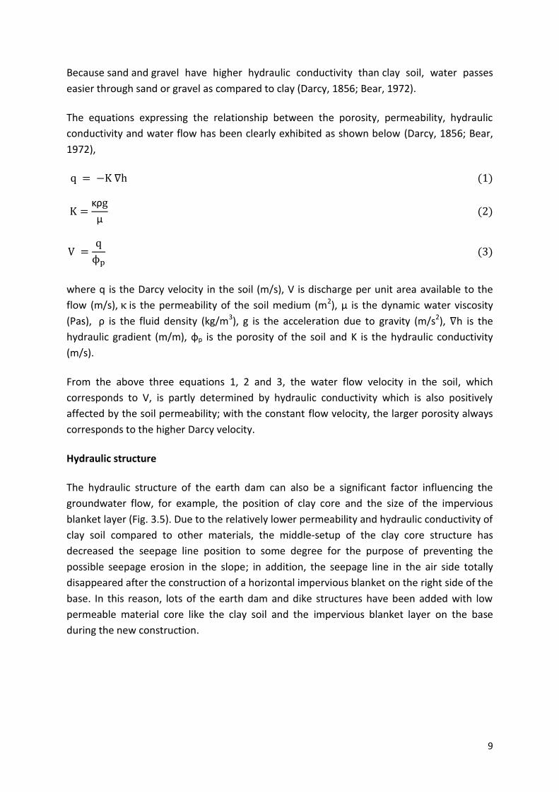
Because sand and gravel have higher hydraulic conductivity than clay soil, water passes

easier through sand or gravel as compared to clay (Darcy, 1856; Bear, 1972).

The equations expressing the relationship between the porosity, permeability, hydraulic

conductivity and water flow has been clearly exhibited as shown below (Darcy, 1856; Bear,

1972),

∇

ρ

where q is the Darcy velocity in the soil (m/s), V is discharge per unit area available to the

flow (m/s), is the permeability of the soil medium (m2), µ is the dynamic water viscosity

(Pa·s), ρ is the fluid density (kg/m3), g is the acceleration due to gravity (m/s2), ∇h is the

hydraulic gradient (m/m), φp is the porosity of the soil and K is the hydraulic conductivity

(m/s).

From the above three equations 1, 2 and 3, the water flow velocity in the soil, which

corresponds to V, is partly determined by hydraulic conductivity which is also positively

affected by the soil permeability; with the constant flow velocity, the larger porosity always

corresponds to the higher Darcy velocity.

Hydraulic structure

The hydraulic structure of the earth dam can also be a significant factor influencing the

groundwater flow, for example, the position of clay core and the size of the impervious

blanket layer (Fig. 3.5). Due to the relatively lower permeability and hydraulic conductivity of

clay soil compared to other materials, the middle-setup of the clay core structure has

decreased the seepage line position to some degree for the purpose of preventing the

possible seepage erosion in the slope; in addition, the seepage line in the air side totally

disappeared after the construction of a horizontal impervious blanket on the right side of the

base. In this reason, lots of the earth dam and dike structures have been added with low

permeable material core like the clay soil and the impervious blanket layer on the base

during the new construction.

10

Case 1: homogeneous earth dam only with toe drain

Case 2: homogeneous earth dam with an additional clay core

Case 3: earth dam with a clay core and horizontal blanket on the base

Fig. 3.5 Comparison of seepage line positions in a homogeneous earth dam with three structures (NPTEL)

Atmospheric condition

Atmospheric condition affecting the hydrological process mainly refers to precipitation

which can increase the water level in the reservoir and can be the driving force for the rising

of potential pressure head difference between the water side and air side of the dam and

increasing of the seepage line in the dam and dike body. In addition, the precipitation has

also direct influence on the water content change with the infiltration water into the

unsaturated slope and then changes the seepage line movement regime especially in an

extreme rainfall event; the rainfall water plays an important role as the direct

supplementary for the groundwater recharge.

Vegetation

The significant influence of vegetation on the hydrological process in the slope can

essentially be attributed to one major aspect: water movement via the soil–plant–

atmosphere continuum (SPAC) (Coppin et al., 1990). Vegetation is a major component of

SPAC, responsible for the suction force of water against gravity. By absorbing parts of the

11

soil water, plants thus play a significant role in the drying of slopes (Huang and Nobel, 1994).

This absorbed soil water will subsequently be removed through the transpiration process

into the atmosphere (Coppin et al., 1990). However this effect can be neglected during the

rainfall season compared with the large amount of infiltrated rain water into the slope.

3.4 Stability problem in the earth dam and dike

3.4.1 Causes of slope landslides

The causes of a landslide are that a landslide occurred in a certain location and at a certain

time. Landslide causes have been detected in various forms showing below:

(1) Rainfall: A long period of rainfall can saturate, soften, and erode soils. Water enters into

existing cracks and may weaken underlying soil layers, leading to failure, for example, mud

slides.

In the majority of cases heavy or prolonged rainfall has been found as the main trigger of

landslides. The rainfall duration and the existing pore water pressure is the direct trigger for

such an event, which can principally be explained by the fact that the rainfall drives the

increase in pore water pressures within the soil. Fig. 3.6(A) exhibits the analysis of the forces

acting on an unstable block on a dam slope without the rainfall infiltration. Movement is

driven by shear stress, which is generated by the mass gravity of the block acting downward

the slope. Resistance to this movement is the result of the normal loading due to the

internal friction. When the slope is filled with infiltrated rainfall water causing the increase of

the groundwater table (Figure 3.6 B), the fluid pressure provides the soil block with a

buoyancy force, which can reduce the friction resistance to the movement of the block

downward the slope. In addition, in some cases when the rainfall event is heavy and

prolonged enough, the increasing groundwater flow can provide additional contribution on

the slope as a result of a hydraulic push to the soil block, which further decreases the

slope stability (Caine, N., 1980; Corominas, J. and Moya, J. 1999).

Fig. 3.6 Diagram illustrating the resistance to, and causes of, movement in a slope system consisting of an

unstable block (A: before a rainfall event; B: during a rainfall event) (Oikos-team, 2007)

12

(2) Steady seepage: As mentioned in the last section, seepage forces in the sloping direction

contribute a push force and add to gravity forces to make the slope susceptible for instability.

The pore water pressure or the buoyancy force decreases the resistance shear strength for

the landslide.

(3) Sudden drawdown of the reservoir water level: This happens mainly due to the man-

made operation of reservoir water release, which results in instability of the water side slope.

With the quick drop of water level, the drop of the seepage line in the dam body shows a

phenomenon of hysteresis and the shearing resistance decreases due to the decrease of soil

resistance parameters (e.g. cohesion, internal friction) accompanying with the quick

dissipation of the hydro-static pressure from the reservoir water; in this case the saturated

slope above the water level is in higher and higher risk of slope slide. In addition, increased

groundwater seepage velocities take place in the event of a sudden fall of the water table in

water reservoirs. If such a slope is formed by unstable soils, suffosion phenomena and

hydrodynamic pressure may cause the occurrence of landslides (Záruba and Mencl, 1987).

(4) External loading: Additional loads (e.g. plant of vegetation) placed on top of the slope

increases the gravitational forces that may cause the slope to fail. Gray and Leiser (1982)

mentioned that the weight of large woody vegetation on a slope might exert a de-stabilizing

stress to a slope. Moreover, the large trees if having been planted on the slope will also

receive a wind-throwing force which is destabilizing influence from turning moments exerted

on the slope as a result of strong winds blowing downward the slope through those trees

(Greenwood et al., 2004); this wind-throwing force provides more negative effects during

the heavier rainfall event which can saturate the slope soils, reduce root adhesion, increase

the weight of trees crowns and thus make those trees more susceptible to collapse

especially accompanying the storm system (Faculty of Geography, University of Victoria).

(5) Surface erosion: The wind and flowing water (e.g. surface runoff of the rainfall water)

causes surface erosion on the top or up surface of the slope and makes the slope steeper

and thereby increases the tangential component of driving force (Menashe, 1998).

(6) Earthquakes: The passage of the earthquake waves through the soil materials produces a

complex set of accelerations which can effectively change the gravitational loading on the

slope of the earth dam. So vertical accelerations successively increase and decrease the

normal loading acting on the slope; similarly, horizontal accelerations induce a shearing

force due to the inertia of the landslide mass during the accelerations. These processes are

complex, but can be sufficient to induce failure of the earth slope. These processes can be

much more serious in mountainous areas in which the seismic waves interact with the

terrain to produce increases in the magnitude of the ground accelerations. This process is

termed 'topographic amplification'. The maximum acceleration is usually seen at the crest of

the slope or along the ridge line, meaning that it is a characteristic of seismically triggered

landslides that extend to the top of the slope (Keefer, 1984).

13

(7) Construction activities at the toe of the slope: Excavation at the bottom of the sloping

surface makes the slopes steep and thereby increases the gravitational forces which may

result in slope failure. In addition, the human constructions on the slope or at the bottom of

the slope could release and loose the subsurface soil compaction, which results in more

possibility of landslides due to groundwater erosion (e.g. backward erosion showing in

Figure 3.7) (Malgot and Baliak, 2002).

Fig. 3.7 Process of backward erosion (Sellmeijer et al., 2011)

3.4.2 Types of slope landslides

The term “landslide” describes a wide variety of processes that result in the downward and

outward movement of slope-forming materials including rock, soil, artificial fill, or a

combination of these. The materials may move by falling, toppling, sliding, spreading, or

flowing. Figure 3.8 shows a graphic illustration of a landslide with the commonly accepted

terminology describing its features (USGS, 2004).

Fig. 3.8 An idealized slump-earth flow showing commonly used nomenclature for labeling the parts of a

landslide (USGS, 2004)

14

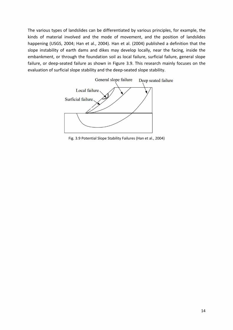
The various types of landslides can be differentiated by various principles, for example, the

kinds of material involved and the mode of movement, and the position of landslides

happening (USGS, 2004; Han et al., 2004). Han et al. (2004) published a definition that the

slope instability of earth dams and dikes may develop locally, near the facing, inside the

embankment, or through the foundation soil as local failure, surficial failure, general slope

failure, or deep-seated failure as shown in Figure 3.9. This research mainly focuses on the

evaluation of surficial slope stability and the deep-seated slope stability.

Fig. 3.9 Potential Slope Stability Failures (Han et al., 2004)

15

Chapter 4 Methodology for Hydrological Process Simulation

The hydrological processes can be simulated by the Program PCSiWaPro® (developed at the

Technische Universität Dresden, Institute of Waste Management and Contaminated Site

Treatment) which describes the distribution of water saturation under transient boundary

conditions in the earth dam (Graeber et al. 2006). With PCSiWaPro® a 2D model of the earth

dam can be built, incorporating information of geometry, soil properties, climate parameters

and geohydraulic and time-dependent boundary conditions.

4.1 General description of the Program PCSiWaPro®

The software PCSiWaPro® is based on solving the Richard’s equation in two spatial

dimensions using the finite element method (Graeber et al. 2006). The integration of a

weather generator into PCSiWaPro® allows a transient flow calculation with respect to

atmospheric conditions (precipitation, evaporation, daily mean temperature and sunshine

duration) and removal of water by plant roots (Hasan et al., 2012). The weather generator's

synthetic time series are statistically derived from publicly available weather station data of

the German Weather Service (DWD) (Hasan et al., 2012). To determine the effects of the

above-mentioned factors on the through-flow and the geomechanical instabilities in the

partially saturated region of the earth dam, the seepage line as the border between the fully

saturated and partially saturated zone in the dam body (Figure 1.1) was used for validating

the simulation results (Hasan et al., 2012). In addition, the water pressure head in the dam

body can be also calculated by PCSiWaPro®; for this, an observation point in the model is

used in order to compare the measured values of the seepage line depth with the simulated

values.

4.2 Theoretical Background of the Program PCSiWaPro®

PCSiWaPro® simulates water flow and contaminant transport processes in variably saturated

soils, under both stationary as well as transient boundary conditions. The flow model can be

described by the Richard’s equation (equation 4).

SKxhKK

xtAiz

j

Aij

i

(4)

The equation contains the volumetric water content θ, hydraulic head h, spatial coordinates

xi (x1 = x and x2 = z for vertical-plane simulation), time t, and KijA

as components of the

dimensionless tensor of anisotropy of hydraulic conductivity K. S is a source/sink term, which

can be partly characterized by the volume of water that is removed from the soil by plant

roots. The effects described by this strongly nonlinear partial differential equation are

subject to hysteresis, especially the relationship between water content and pressure head

16

(Hasan et al., 2012). This relationship can be described by the van-Genuchten-Luckner

equation (5).

nnc

lrrr

h11

,

1

(5)

where Φ is the porosity of the soil; r is residual water content; r,l is residual air content; hc

characterizes the pressure head difference between the wetting (water) and non-wetting

phase (air); α (scale factor) and n (slope) are empirical van-Genuchten parameters

(Kemmesies, 1995). The simulation tool PCSiWaPro® implements this relationship and solves

the RICHARDS equation in two vertical-plane dimension with transient boundary conditions,

using a numerical finite element approach. For the solution of the linear system of equation

originating from discretizing the Richard’s equation, an iterative preconditioned conjugate

gradient solver is used (Hasan et al., 2012).

4.3 Advantage of the Program PCSiWaPro®

Although there are several available programs for the hydrological process simulation, for

example, Hydrus and Feflow, the program PCSiWaPro® does have some advantages in the

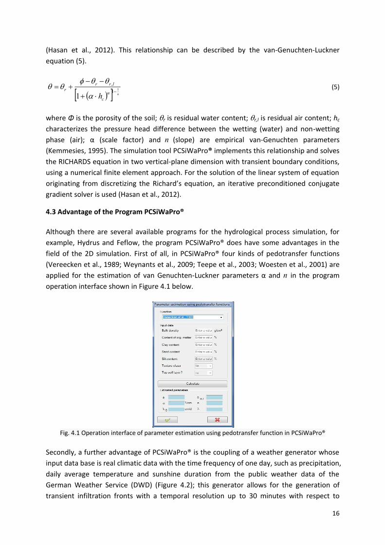
field of the 2D simulation. First of all, in PCSiWaPro® four kinds of pedotransfer functions

(Vereecken et al., 1989; Weynants et al., 2009; Teepe et al., 2003; Woesten et al., 2001) are

applied for the estimation of van Genuchten-Luckner parameters α and n in the program

operation interface shown in Figure 4.1 below.

Fig. 4.1 Operation interface of parameter estimation using pedotransfer function in PCSiWaPro®

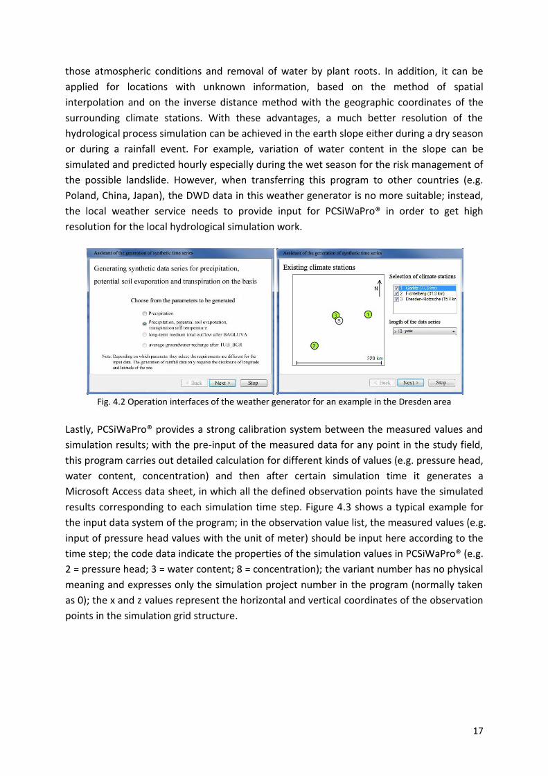
Secondly, a further advantage of PCSiWaPro® is the coupling of a weather generator whose

input data base is real climatic data with the time frequency of one day, such as precipitation,

daily average temperature and sunshine duration from the public weather data of the

German Weather Service (DWD) (Figure 4.2); this generator allows for the generation of

transient infiltration fronts with a temporal resolution up to 30 minutes with respect to

17

those atmospheric conditions and removal of water by plant roots. In addition, it can be

applied for locations with unknown information, based on the method of spatial

interpolation and on the inverse distance method with the geographic coordinates of the

surrounding climate stations. With these advantages, a much better resolution of the

hydrological process simulation can be achieved in the earth slope either during a dry season

or during a rainfall event. For example, variation of water content in the slope can be

simulated and predicted hourly especially during the wet season for the risk management of

the possible landslide. However, when transferring this program to other countries (e.g.

Poland, China, Japan), the DWD data in this weather generator is no more suitable; instead,

the local weather service needs to provide input for PCSiWaPro® in order to get high

resolution for the local hydrological simulation work.

Fig. 4.2 Operation interfaces of the weather generator for an example in the Dresden area

Lastly, PCSiWaPro® provides a strong calibration system between the measured values and

simulation results; with the pre-input of the measured data for any point in the study field,

this program carries out detailed calculation for different kinds of values (e.g. pressure head,

water content, concentration) and then after certain simulation time it generates a

Microsoft Access data sheet, in which all the defined observation points have the simulated

results corresponding to each simulation time step. Figure 4.3 shows a typical example for

the input data system of the program; in the observation value list, the measured values (e.g.

input of pressure head values with the unit of meter) should be input here according to the

time step; the code data indicate the properties of the simulation values in PCSiWaPro® (e.g.

2 = pressure head; 3 = water content; 8 = concentration); the variant number has no physical

meaning and expresses only the simulation project number in the program (normally taken

as 0); the x and z values represent the horizontal and vertical coordinates of the observation

points in the simulation grid structure.

18

Fig. 4.3 An example of the input system interface of the measured pressure head data for the observation

point (470, 15.2)

4.4 Model Setup of an earth dam in PCSiWaPro®

Before the start of the PCSiWaPro® simulation, the various initial and boundary conditions in

the earth dams should be identified and then defined in the program. The initial condition is

either the distribution of the pressure head or the water content in the whole dam area. This

program can be used under various boundary conditions, e.g. time-dependent boundary

conditions, atmospheric boundary conditions, seepage face. Time-dependent boundary

conditions are defined by measured water levels at the water side of the dam. Furthermore

atmospheric boundary conditions like precipitation or evapotranspiration can be applied. At

the air side of the dam a seepage face was defined to allow outflow only when the soil has

reached full water saturation (Hasan et al., 2012).

Figure 4.4 shows an example of boundary condition setup for a physical earth dam with a

rubber wall in the middle. On the foot of the left side, there is a yellow line with boundary

condition of time dependent potential head which means that this layer has an influence of

transient flooding level; on the left slope and in the middle there are impermeable walls

allowing no water flux through these two layers; the red vegetation line on the top and on

some part of the right slope has atmospheric boundary condition, and can be infiltrated

through by rainfall water; lastly the blue line on the foot of the right slope means the

seepage face.

Fig. 4.4 Setup of various boundary conditions in the program PCSiWaPro®

19

After setting up the boundary conditions, the parameters of the earth dam materials (dam

slope, core if possible, foundation materials, soil materials beyond the dam area) need to be

input into PCSiWaPro® (Figure 4.5). There can be either input from the soil parameter data

which have been achieved from the field or laboratory investigation or easily input from the

existing soil database DIN4220 which has been installed into the program.

Fig. 4.5 Input of the soil parameters into the program PCSiWaPro®

Discretization of the model area is required for the calculation with the program PCSiWaPro®.

In this case, unstructured triangular mesh elements can be specified. This enables the user

to adequately map even irregular model areas. The implemented mesh generator uses the

"Boundary Representation Modeling Technique" and therefore requires the specification of

the model boundaries (Hasan et al., 2012). Since the range of the dam embankment is of

interest for the evaluation, this section of the model is discretized finer (10 cm), which

results in a better representation of the change in water contents in the unsaturated zone

above the seepage line and enables a better comparison between simulated and measured

values.

20

CHAPTER 5 Methodologies for Stability Analysis

5.1 Factor of safety (Fs)

The factor of safety value for stability analysis is the primary index to determine how close or

far the slope is from failure; and the minimum Fs value is taken as a basic index for the safe

engineering design. The classical approach used in designing engineering structures (e.g.

the earth dam slope) is to consider the relationship between the shear strength or

resisting force of the element and the stress for the slope balance required (equation 6).

Fs =

=

(6)

The total shear strength inside the soil indicates the shear strength due to the different soil

properties, i.e. the soil cohesion, internal friction and matric suction; the detailed calculation

will be discussed in the sections; while the shear stress required for the balance is mainly

caused by the weight of soil and water which is the downward component of the total soil-

water weight along the slope.

Failure is assumed to occur when Fs is less than a certain value (normally one). The

determination of the recommended Fs values is usually based on various factors, for

example, soil types, engineering structures, failure modes. Table 1 shows the recommended

Fs values for the design of different engineering foundation structures. And in this table, the

reference Fs value for the earth dams under the mode of the shear stress analysis will be

focused on and applied to the stability analysis in this research.

Table 1 Typical values of customary safety factors, Fs, as presented by Bowels (1988).

Failure Mode Foundation Type Fs

Shear Earthwork for Dams, Fills, etc. 1.2 - 1.6

Shear Retaining Walls 1.5 - 2.0

Shear Sheetpiling, Cofferdams 1.2 - 1.6

Shear Braced Excavations

(Temporary) 1.2 - 1.5

Shear Spread Footings 2 – 3

Shear Mat Footings 1.7 - 2.5

Shear Uplift for Footings 1.7 - 2.5

Seepage Uplift, heaving 1.5 - 2.5

Seepage Piping 3 – 5

5.2 The basic Mohr-Coulomb Model

The total shear strength in the soil can be calculated by the Mohr–Coulomb theory which is a

mathematical model describing the response of brittle materials such as concrete, or soils, to

shear stress as well as normal stress. Most of the classical engineering materials somehow

follow this rule in at least one portion of their shear failure envelope. Generally the theory

21

applies to materials for which the compressive strength far exceeds the tensile strength

(Juvinal and Marshek, 1991).

5.2.1 Theoretical background

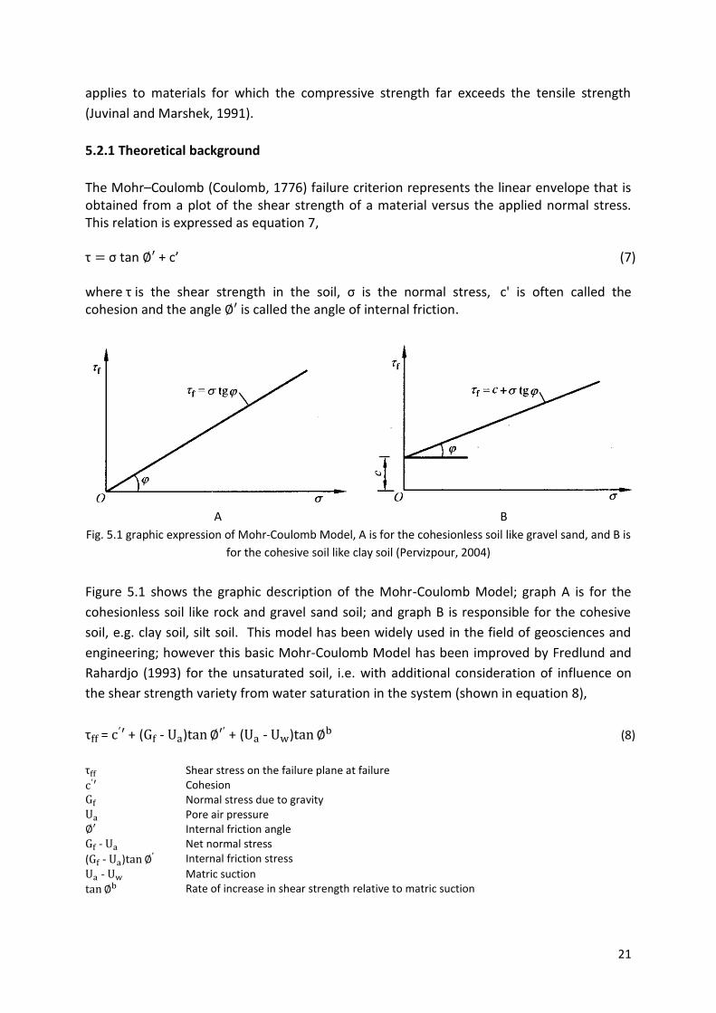
The Mohr–Coulomb (Coulomb, 1776) failure criterion represents the linear envelope that is obtained from a plot of the shear strength of a material versus the applied normal stress. This relation is expressed as equation 7,

σ tan + c’ (7)

where is the shear strength in the soil, σ is the normal stress, c' is often called the cohesion and the angle is called the angle of internal friction.

A B

Fig. 5.1 graphic expression of Mohr-Coulomb Model, A is for the cohesionless soil like gravel sand, and B is

for the cohesive soil like clay soil (Pervizpour, 2004)

Figure 5.1 shows the graphic description of the Mohr-Coulomb Model; graph A is for the

cohesionless soil like rock and gravel sand soil; and graph B is responsible for the cohesive

soil, e.g. clay soil, silt soil. This model has been widely used in the field of geosciences and

engineering; however this basic Mohr-Coulomb Model has been improved by Fredlund and

Rahardjo (1993) for the unsaturated soil, i.e. with additional consideration of influence on

the shear strength variety from water saturation in the system (shown in equation 8),

= + ( - ) + ( - ) (8)

Shear stress on the failure plane at failure

Cohesion Normal stress due to gravity Pore air pressure Internal friction angle - Net normal stress

( - ) Internal friction stress

- Matric suction

Rate of increase in shear strength relative to matric suction

22

With the modified Mohr-Coulomb Model, the shear strength of an unsaturated soil can be

formulated in terms of independent stress state variables (Fredlund et al., 1978); the stress

state variables, ( - ) and (Ua - Uw), have been exhibited to be the most advantageous

combination for practical purpose (Fredlund et al., 1978).

In most of the geotechnical researches, the parameters of cohesion (c’) and internal friction

angle ( ) have been conventionally taken as a constant for the stability analysis (Zhou,

1990); however they do vary as the parameter of matric suction according to the water

saturation change in the materials. Lv et al. (2010) did a research about the different effects

of the soil parameters on the slope stability and they found that the parameter of cohesion,

internal friction angle and matric suction were among the most important factors. In this

case, the study of the relationships between water saturation change and variety of those

parameters is in great need.

5.2.2 Cohesion (c’) change related to soil water content

The properties of granular material (like soils) can be significantly influenced by the cohesion

forces between particles; for example, it is well known that the angle of repose of a wet pile

is greater than that of a dry pile made of the same material, which makes sand castles

possible (Li, 2005). Cohesion can arise from a variety of sources: mainly liquid bridging

(capillary) forces, Van der Waals forces, electrostatic forces (Israelachvelli, 1991). In the

section 5.2.3, the capillary force (or called matric suction force) will be separately discussed

in the modified Mohr-Coulomb Model. In the actual section, Van der Waals forces and

electrostatic forces are taken as the only two main sources of the soil cohesion.

Van der Waals interactions are the sum of the attractive or repulsive forces between

molecules (or between parts of the same molecule) other than those due to covalent bonds,

or the electrostatic interaction of ions with one another, with neutral molecules, or with

charged molecules (IUPAC, 1997). The electrons in an atom can arrange themselves

anywhere within their orbitals, and may group toward one side of the molecule, thus

creating a temporary slight negative charge on one side and a positive one on the other side

(Israelachvili, 1990); Van der Waals forces are a kind of interaction resulting from the inter-

particle spacing at the molecular level (Nase, 2000). When the distance of molecules

increases, attraction force takes place; while the molecules get closer, the electron clouds

associated with the molecules overlap, and hence repulsion comes out (Li, 2005). Van der

Waals forces are relatively weak compared to covalent bonds, hydrogen bonds and

electrostatic forces, but play a fundamental role in several fields, like in the soil-water

system. Van der Waals force is one kind of cohesion source although contributing only a

little; compared with other cohesion sources (like the hydrogen bonds discussed later), this

contribution force can be assumed to be a constant with the variety of water content in the

soil-water system.

In addition, the electrostatic forces can arise through friction (i.e., tribocharging) that leads

23

to electrostatic charging of the objects, due to the electron transfer between objects

(Rhodes, 1998). In the soil-water system, the most common electrostatic force is from

hydrogen bonds occurring between polar molecules when a hydrogen (H) atom bound to a

more electronegative oxygen atom (O) experiences attraction to some other highly

electronegative atom nearby (Arunan et al., 2011). The hydrogen bond is stronger than the

van der Waals interaction (IUPAC, 1997) and is the direct source of surface tension, stronger

hydrogen bonds always corresponding to more powerful surface tension. In addition,

another source of electrostatic force is mainly due to charged ions in soil water, like heavy

metal ions and Nitrate ions, which is stronger than the hydrogen bonds (IUPAC, 1997);

however in this study the quantity of charged ions and the influence on the cohesion is so

little that the contribution from these ions can also be taken as a constant with the water

saturation change.

In conclusion, the variety of soil cohesion is mainly determined by surface tension which is

mainly originated from hydrogen bonds with water saturation change; electrostatic

attraction between charged ions in the soil-water system have also contributed to cohesion

although this contribution is small can be assumed to be constant or even sometimes

negligible, as having been clearly declared in equation 9.

Cohesion force C = Electrostatic force + Van der Waals forces (9)

≈surface tension force + constant cohesion force part (negligible)

The cohesion force of water binding the two particles (Figure 5.2) due to the surface tension

can be achieved by equation 10 displayed below,

Fc = 2 π σt (10)

Fig. 5.2 Idealized particles held together by water (Kemper and Rosenau, 1984)

where Fc presents the cohesion force, σt is the surface tension of the air-water interface in

24

N/m and is the length (m) of that air-water interface in the jth pore space acting to pull the

particles together. However in the real soil-water system, the sizes of pore air and water

volumes are not uniform from each other (Figure 5.3); for the total cohesion force in the

soil-water system, Kemper and Rosenau (1984) further improved equation 10 into equation

11 with additional consideration of the randomness of those different pore sizes,

Fc = 2 π σt (11)

where n is the total number of pore spaces.

Fig. 5.3 Pore air and water volume (Bellingham, 2009)

Since now a lot of researches have studied the relationship between the cohesion and soil

water content; and most of the results indicate a negative relationship between them. For

example, Kim et al. (2011) had a field experiment with three different soils displayed in

Figure 5.4 and found that the higher soil water saturation was followed by the lower soil

cohesion, which was also proved by Tang et al. (2012).

Fig. 5.4 Experimental result of the relationship between cohesion and saturation of different types of soils

(Kim et al., 2011)

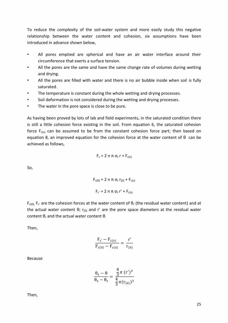
25

To reduce the complexity of the soil-water system and more easily study this negative

relationship between the water content and cohesion, six assumptions have been

introduced in advance shown below,

• All pores emptied are spherical and have an air water interface around their

circumference that exerts a surface tension.

• All the pores are the same and have the same change rate of volumes during wetting

and drying.

• All the pores are filled with water and there is no air bubble inside when soil is fully

saturated.

• The temperature is constant during the whole wetting and drying processes.

• Soil deformation is not considered during the wetting and drying processes.

• The water in the pore space is close to be pure.

As having been proved by lots of lab and field experiments, in the saturated condition there

is still a little cohesion force existing in the soil. From equation 6, the saturated cohesion

force Fc(s) can be assumed to be from the constant cohesion force part; then based on

equation 8, an improved equation for the cohesion force at the water content of θ can be

achieved as follows,

Fc = 2 n π σt r + Fc(s)

So,

Fc(0) = 2 n π σt r(0) + Fc(s)

Fc’ = 2 n π σt r’ + Fc(s)

Fc(0), Fc’ are the cohesion forces at the water content of θr (the residual water content) and at

the actual water content θ; r(0) and r’ are the pore space diameters at the residual water

content θr and the actual water content θ.

Then,

Because

Then,

26

So

c'0, c’ and c’s are the cohesion at the water content of θr (the residual water content), θ and

θs (the saturated water content);

Then a new model describing the relationship between the water content and soil cohesion

has been developed here,

– (12)

θ water content in the soil θ saturated water content θ residual water content c‘ soil cohesion at water content θ c’0 soil cohesion with the residual soil water content of θr c'S soil cohesion with full water saturation θS

c'0 and c’s can be achieved from lab experiments (e.g. triaxial test) or from the existing

research results, e.g. Tables 1- 3 in Appendix.

5.2.3 Matric suction (Ua – Uw) change due to water content change

As mentioned in the last section, the capillary force or matric suction force is another

significant factor influencing the unsaturated soil properties. Matric suction force is induced

by liquid bridges formed between particles and created by the pressure difference (Ua-Uw)

across the air-liquid interface (Rhodes, 1998). The mechanism that leads to slope failures is

the matric suction that starts to decrease when water begins to infiltrate the unsaturated

soil. The loss of matric suction decreases the shear strength of the soil below the mobilized

shear strength along the potential slip surface (Yeh et al., 2008). In order to determine the

exact influence from the matric suction on the slope stability, the important relationship

between the matric suction of the soil and the water content is beforehand required for the

unsaturated soil mechanics. This relationship is called the soil water characteristic curve

(SWCC) showing the ability of an unsaturated soil to retain water under various matric

27

suctions (Fattah et al., 2013) and can be obtained in the laboratory using a pressure plate

test (Yeh et al., 2008). The common result from the SWCC is that the matric suction

increases as the degree of saturation (or water content) decreases in different kinds of soils;

Figure 5.7 represents one example.

Fig. 5.7 Soil-water characteristic curve of fine sand (i.e. tailings) (Gonzalez and Adams, 1980)

From the van Genuchten-Luckner equation, the relationship between water content and matrix suction can be easily achieved, displayed as equation 13;

(Ua - Uw) = ρgΨ = ρg

(13)

α - scaling factor n - slope factor Ψ - matric suction ρ - density of water g - earth gravitational acceleration

Parameters α and n can be precisely derived in the laboratory experiment.

From equation 13 it can be easily understood that when the soil is fully saturated, the matric

suction is equal to 0. Matric suction is a critical factor affecting the slope stability. Hossain

(2010) undertook a field experiment in a residual granite soil slope and obtained (Figure 5.8)

that the slope could be more stabilized with more matric suction.

28

Fig. 5.8 Effect of matric suction on factor of safety in a residual granite soil slope (Hossain, 2010)

5.2.4 Internal friction change due to water content change

The soil internal friction angle describes the soil friction characteristics, and generally it can

be divided into two parts, the surface friction between soil particles and the interlocking

force between particles (Shi et al., 2011). In most geosciences researches, internal friction

angle of soil has been always taken as a constant; however it does change due to some

factors, for example, the water saturation, soil density, structure, size and shape of soil

particles, and degree of compaction (Shi et al., 2011). In order to simplify this research work,

the influence from the water saturation is only considered and that from the other factors is

taken as a constant. Deng et al. (2008) found that the internal friction angle of the soil

decreased with the increase of water content and it decreased to a greater extent especially

when soil water content was greater than 10%. Kim et al. (2011) got a result from a field

experiment with three types of soils that there was a negative correlation between soil

internal friction angle and soil water saturation (figure 5.9).

Fig. 5.9 Experimental results of the correlation between internal friction and saturation for three types of

soils (Kim et al., 2011)

More detailed, from the laboratory experiment result shown in figure 5.10, Shi et al. (2011)

developed a simple model (equation 14) for the negative relationship between the internal

friction and water saturation in the Guiyang red clay.

29

ln = - 0.005·w + 2.60 (14)

w --- water saturation in the soil (= θ θ

)

Fig. 5.10 Relation between the internal friction angle and water saturation (Shi et al., 2011)

In geo-science practices, equation 14 is convenient and applicable for the fast decision

support for the certain soil of Guiyang red clay; however it neglects the influence of the

variety of different soils, which causing unsuitability for other soil types.

Similarly, Bian and Wang (2011) ran a field experiment with three kinds of soils and derived

that there was a linear relationship between the water content and the internal friction

angle (equation 15).

’(θ) = a·θ + b (15)

a, b --- fitting parameters of the linear relationship curve

Depending on equation 15, the internal friction angle at the residual water content θ

and at the saturated water content θ can be obtained as

= a θ + b

= a θ + b

Then by solving those above two equations, the parameters a and b can be achieved as

shown below,

θ θ

θ θ

θ

30

So,

-

θ +

=

Then this linear relationship can be modified into:

= tan (

) (16)

r -- soil internal friction angle with the residual water content of

s -- soil internal friction angle with the saturated water content of

In the laboratory, r and s can be easily achieved by the shear test (the direct shear test or

triaxial shear test) or from the soil data-bases like Table 4 shown in Appendix. With another

two known values for soil-water parameters ( and ), equation 16 can be easily applied

for all kinds of soils.

5.2.5 change due to the water content change

expresses the shear strength contribution due to suction (equation 17) and it can be

predicted by the soil-water characteristic curve. Vanapalli et al. (1996) promoted a

laboratory experiment which could approximately express the relationship between

and water content change in the unsaturated soil (shown in Fig. 5.11); and then they

developed a model to express the relationship between and water saturation

(equation 18).

=

(17)

Fig. 5.11 Variation of shear strength with respect to matric suction (Vanapalli et al., 1996)

31

= θ θ

θ θ (18)

From Fig. 5.11, it can be seen that larger matric suction and less water content correspond to

smaller , which exhibits a positive relationship between the water content and .

Then combining equations 16 and 18, this clear positive relationship between and

water content can be given as equation 19,

= θ θ

tan (

) (19)

The values of θs, θr, Ø’r, and Ø’s can be achieved beforehand from the experiment or by

looking through the soil data; then this relationship equation is only a function of the real

water content in the soil.

5.3 Influence of vegetation on the slope stability

The relationship between vegetation and slope stability is determined by the abilities of the

plant life growing on slopes to strengthen the stability; there are mainly two kinds of abilities

of vegetation influencing the slope stability, i.e. hydrological effect (removal of water) and

root reinforcement.

5.3.1 Hydrological effects of vegetation

Vegetation provides a protective layer or buffer between the atmosphere and the soil.

Through the hydrological cycle, it influences the transfer of water between the atmosphere

and the earth’s surface and underground soil, which therefore affects the volume of soil

water storage (Styczen and Morgan, 1995).

Vegetation influences slope stability by removing water through transpiration. Transpiration

is the vaporization of liquid water contained in the plant and the vapour removal to the air

(FAO, 2007). Water moves via the soil–plant–atmosphere continuum (SPAC) (Coppin et al.,

1990) and vegetation is a major component of SPAC, responsible for the suction force of

water against gravity. By absorbing parts of the soil water, plants thus play a significant role

in the drying of slopes (Huang and Nobel, 1994). This absorbed soil water will subsequently

be removed through the transpiration process into the atmosphere, of which the major

effect is the reduction of soil pore water pressures counteracting the loss of strength

occurring during wetting (Coppin et al., 1990; FAO, 2007; Greenwood et al., 2004).

Ultimately, this water cycle system will result in less saturated and more stable slopes.

Transpiration is accentuated when the vegetation has an extensive root system (Perry et al.,

2003) and then slope stability can be promoted. Osman and Barakabah (2006) have carried

out a few studies in Malaysia which showed that there was a significant relationship

32

between root length density, soil water content and slope stability. They found that slopes

with high root density were less likely to experience slope failure, which could be explained

by the fact that a high root length density results in the low soil water content, in turn

resulting in an increase in shear strength and a decrease in soil permeability.

In addition, during the wet season the removal of water from the soil surface (evaporation)

can be reduced by the shading provided by vegetation, resulting in a negative influence on

the slope stability. As mentioned above, less water content is more beneficial for a stable

slope; this reduction of evaporation can keep the water saturation in the surface layer of the

slope at a high degree, which causes a high risk of surficial slope slides during the next

extreme rainfall event. In contrast, in the dry season the slope can be more stabilized by the

shading of vegetation; shading can decrease the rate of evaporation and help to prevent the

desiccation, shrinkage and cracking of the soils, allowing the deep penetration of rain water

(Perry et al., 2003).

5.3.2 Root reinforcement cohesion

The effect of vegetation (grasses, shrubs, or trees) root reinforcement shown in Figure 5.12

on slope stability has been well recognized and incorporated in soil-bioengineering practice

(e.g. Gray and Leiser, 1982; Coppin and Richards, 1990; Gray and Sotir, 1996). Quantitative

studies on this role of vegetation roots on slope stability have been carried out about 40

years ago with shear tests performed on soil blocks containing roots; the shear strengths in

the tests needed for those soil blocks were substantially larger than those for soils without

roots (Endo and Tsuruta, 1969; O'Laughlin, 1974; Ziemer, 1981; Nilaweera, 1994). From field

experiments Swanston (1974), Gray and Megahan (1981), and Tsukamoto and Kusaba (1984)

similarly concluded that clearing of forested slopes increased the frequency of landslides.

Fig. 5.12 Plant reinforcement in riprap and small fills (Leiser, 1998)

33

To evaluate the root reinforcement in detail, material properties and analytical models are

essential components; Wu (2013) developed an analytical model shown in equations 20 and

21 with a commonly used property σ which is the tensile strength of the root material and

can be measured by performing a simple tension test on a root segment.

RAR =

=

(De Baets et al., 2008) (20)

≈1.2

(Wu, 2013) (21)

RAR root area ratio cohesion due to roots the number of roots in each root diameter class mean root cross-sectional area of a root diameter class A reference area, vertical projection of the above-ground biomass of the plant Ar root area σ tensile strength of the root material

can also be derived from some literatures, for example, from the experiment of

Hoffmans et al. (2010) (Table 5 in Appendix), where is found to be ca. 2*107 N/m2;

Morgan and Rickson (1996) made a table for tensile strength of different roots collected

from different literatures (Table 6 in the Appendix).

In addition, the parameter of root area ratio ( ) can be achieved by the simple sampling

measurement in the field practice or approximately be derived from the existing research

results for different vegetation covers, e.g. Tables 7 and 8 shown in Appendix.

5.4 The Infinite Slope Model for the surficial landslides

Slope stability problems of dams and dikes are among the most commonly encountered

problems in geotechnical and hydraulic engineering. Numerous scientists conducted a large

amount of research in this field and several numerical methods were developed for the

slope stability analysis with the help of the famous Mohr-Coulomb Model. The typical

methods are the infinite slope equation and the limit equilibrium analysis methods, e.g.

Ordinary Method of Slices, Janbu’s Simplified Method, and Morgenstern-Price method

(Hammond et al., 1992; Biondi, 2000).

The well known infinite slope model is the oldest and simplest mechanical approach for

slope stability which is usually implemented with the following assumptions (Skempton and

DeLory, 1957; Hammond et al., 1992; Biondi, 2000),

- slope extent is infinite or much larger than the depth of potential slip surface;

- slope angle is constant;

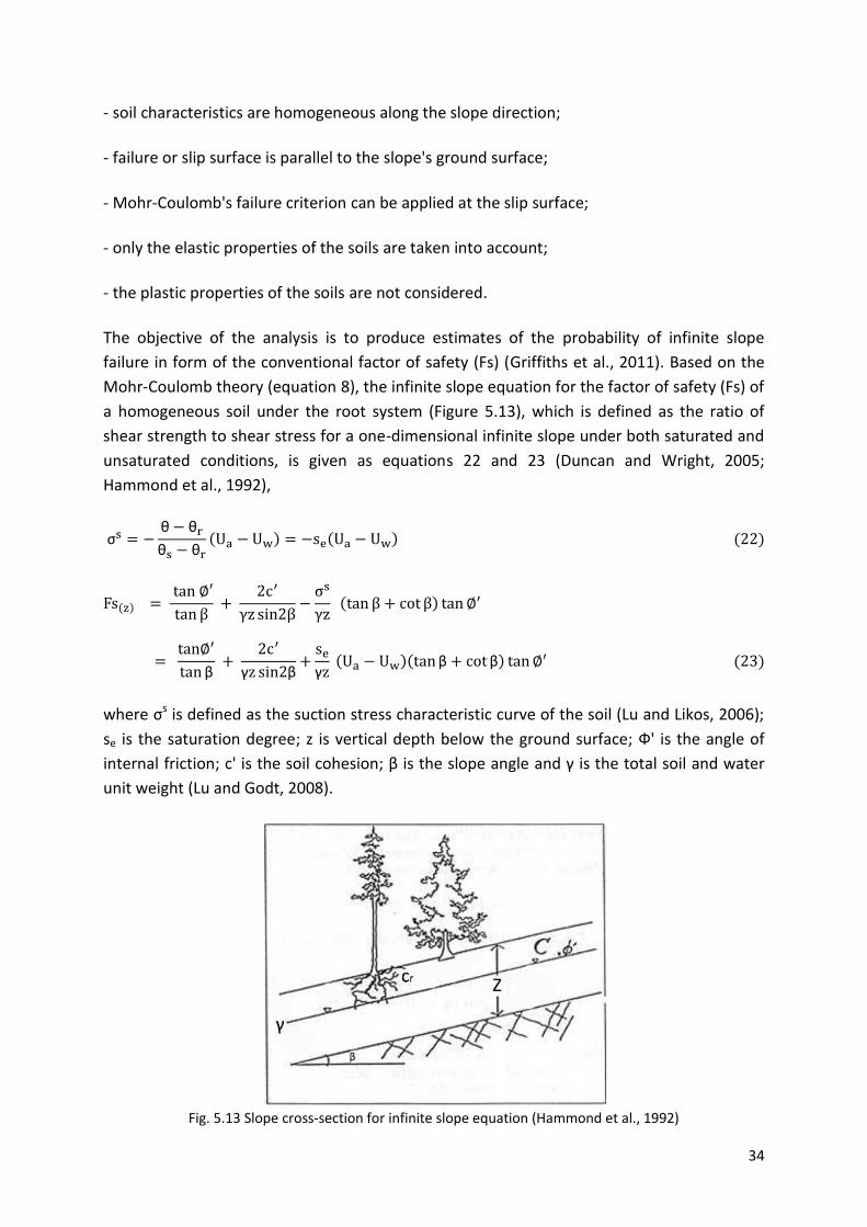
34

- soil characteristics are homogeneous along the slope direction;

- failure or slip surface is parallel to the slope's ground surface;

- Mohr-Coulomb's failure criterion can be applied at the slip surface;

- only the elastic properties of the soils are taken into account;

- the plastic properties of the soils are not considered.

The objective of the analysis is to produce estimates of the probability of infinite slope

failure in form of the conventional factor of safety (Fs) (Griffiths et al., 2011). Based on the

Mohr-Coulomb theory (equation 8), the infinite slope equation for the factor of safety (Fs) of

a homogeneous soil under the root system (Figure 5.13), which is defined as the ratio of

shear strength to shear stress for a one-dimensional infinite slope under both saturated and

unsaturated conditions, is given as equations 22 and 23 (Duncan and Wright, 2005;

Hammond et al., 1992),

σ θ θ

θ θ

β

γ β γ β β

where σs is defined as the suction stress characteristic curve of the soil (Lu and Likos, 2006);

se is the saturation degree; z is vertical depth below the ground surface; Ф' is the angle of

internal friction; c' is the soil cohesion; β is the slope angle and γ is the total soil and water

unit weight (Lu and Godt, 2008).

Fig. 5.13 Slope cross-section for infinite slope equation (Hammond et al., 1992)

35

However, for the Fs value within the root area, the root reinforcement should be considered:

γ β β

cr is the root reinforcement cohesion which can be derived by equation 21. In the

unsaturated slope, the influence of water content on the cohesion, matric suction and

internal friction angle should be included into this old infinite slope model and the detailed

relationships between water content and those soil properties can be achieved by equations

12, 13 and 16. In addition, as can be seen in equation 24, there is only one variable

parameter (i.e. volumetric water content, θ) at the right side for a certain slope stability

analysis, which indicates that the factor of safety for this certain slope is only determined by

the soil-water content in the slope.

5.5 Bishop’s Model for deep landslides

Compared to the infinite slope analysis, the traditional limit equilibrium method is more

common nowadays for the slope stability analysis in the geo-engineering, especially for the

deep seated landslides forecasting (Gover and Hammah, 2013).

Before the start of the limit equilibrium analysis, four assumptions should be checked:

- Mohr-Coulomb's failure criterion can be applied on the slip surface;

- neglecting external horizontal loads (including earthquake loads)

- only consideration of the elastic properties of the soils and no consideration of the plastic

properties of the soils

- the expansion effect of clay soil is neglected.

The typical limit equilibrium analysis methods are Bishop’s Method, Janbu’s Method,

Spencer Method, Morgenstern-Price Method and so on (Krahn, 2004). Among those slope

stability analysis methods, Bishop’s method is one of the best and most convenient ways to

be applied in practice, especially in the case of circular types of sliding surfaces (displayed in

Figure 5.14). In the 1950s Bishop devised this method which included the normal forces inter

the slices from the dividing of the possible circle sliding surface (shown in Figures 5.14 and

5.15), but ignored the inter slice shear forces. Bishop developed an equation for the normal

forces at the slice base by summing slice forces in the vertical direction. The consequence of

this is that the base normal becomes a function of the factor of safety. This in turn makes the

factor of safety equation nonlinear and an iterative procedure is consequently required to

compute the factor of safety (Krahn, 2004).

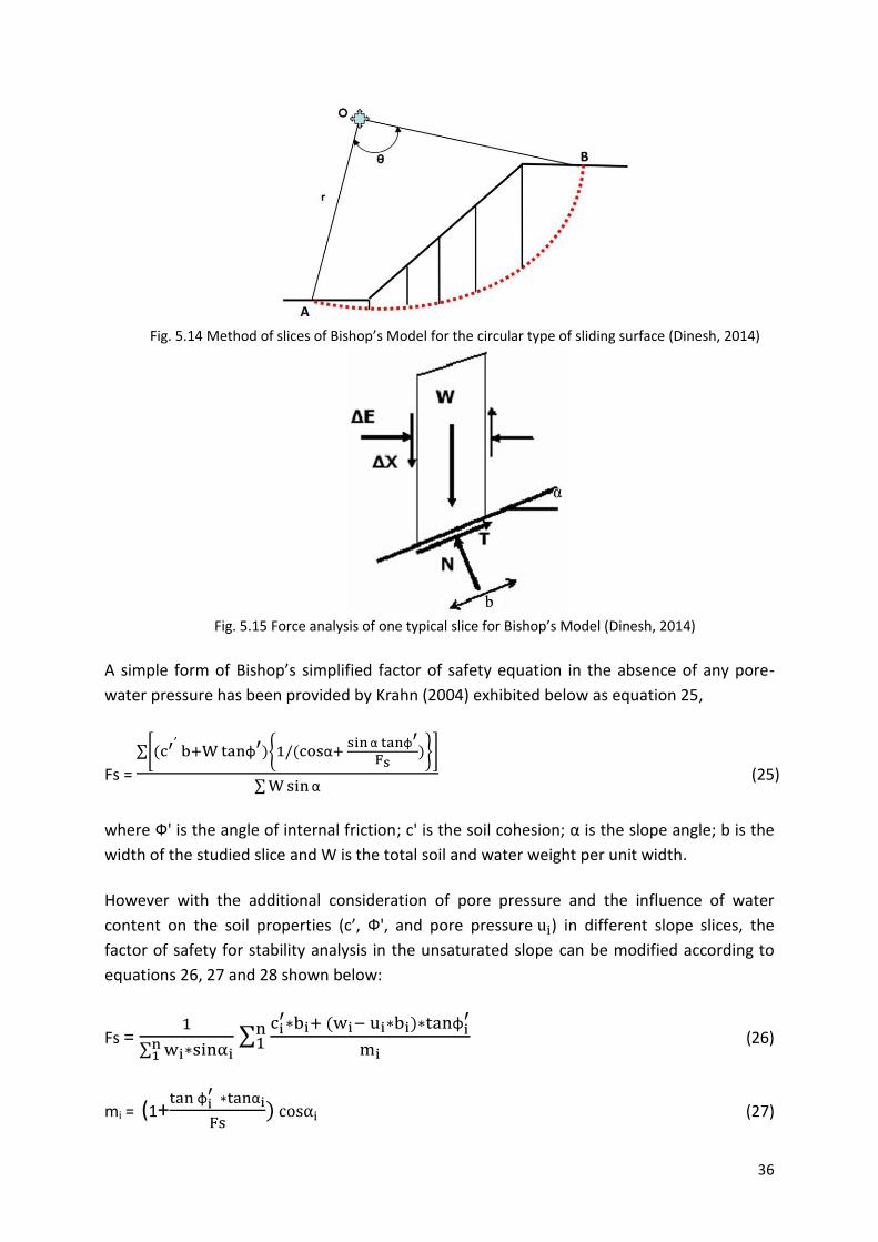
36

Fig. 5.14 Method of slices of Bishop’s Model for the circular type of sliding surface (Dinesh, 2014)

Fig. 5.15 Force analysis of one typical slice for Bishop’s Model (Dinesh, 2014)

A simple form of Bishop’s simplified factor of safety equation in the absence of any pore-

water pressure has been provided by Krahn (2004) exhibited below as equation 25,

Fs =

φ α

α φ

α (25)

where Ф' is the angle of internal friction; c' is the soil cohesion; α is the slope angle; b is the

width of the studied slice and W is the total soil and water weight per unit width.

However with the additional consideration of pore pressure and the influence of water

content on the soil properties (c’, Ф', and pore pressure ) in different slope slices, the

factor of safety for stability analysis in the unsaturated slope can be modified according to

equations 26, 27 and 28 shown below:

Fs =

φ

(26)

mi = (1+ φ

α

(27)

37

= θ θ

θ θ (28)

cohesion of the ith slice, depending on the saturation φ

internal friction angle of the ith slice, depending on the saturation

the angle between the shear force on the ith slice and horizontal face total soil-water weight of the ith slice width of the ith slice pore pressure in the ith slice, depending on the saturation

Pore pressure can be derived from Lu and Likos (2006).

Additionally, in the saturated area of the slope (under the groundwater table) saturated

cohesion and internal friction angle are applied in stability analysis; then Fs can be obtained

by equations 29 and 30,

Fs =

φ

(29)

= (30)

saturated pore water pressure under the seepage line height of the unsaturated part above the seepage line in the ith slice saturated cohesion φ saturated internal friction angle total weight of soil and unsaturated water in the ith slice total height of the ith slice rw unit weight of water

To solve BISHOP’S Model shown in equations 29 and 30, it is necessary to begin with an

assumption for the Fs value; by equation 27 the initial assumption for the Fs value will be

used to calculate mi and then through equation 29, a new Fs value is provided. This

procedure is repeated until the last computed Fs value differs only within a specified

tolerance (e.g. a difference of 0.001) from the previous Fs value; fortunately, this work can

be finished only by a few iterations to reach a converging solution (Krahn, 2004).

5.6 Application of the GEO-SLOPE Program

5.6.1 Description of the GEO-SLOPE Program

Since now various computer-based geotechnical softwares have been developed and

performed for the slope stability analysis; and those geo-softwares mainly utilize two

methodologies, the limit equilibrium models and the finite element analysis based on

appropriate soil models which arouse great interest both of researchers and of professionals.

Among those softwares, a computer software SLOPE/W is one of the best and has been

developed by Fredlund at the University of Saskatchewan. SLOPE/W is one component in a

complete suite of geotechnical products called GEO-SLOPE, one of whose powerful features

38

of the integrated approach is that it opens the door to types of analyses of a much wider and

more complex spectrum of problems, including the use of finite element computed pore-

water pressures and stresses in a stability analysis (Krahn, 2004). In addition, in SLOPE/W

four kinds of the limit equilibrium methods are available; these are Ordinary Method,

Bishop’s Method, Janbu Method and Morgenstern-Price Model; however in this doctor

thesis only the results from Bishop’s Method are discussed for the further improvement

application for the earth dam stability analysis.

When the stability of slope is calculated by using Bishop’s method, the most prominent

problem is confirmation of the critical slip surface in the slope in order to forecast the

coming landslide in the deep layer. The critical slip surface in slope stability analysis is the

surface that produces the minimum factor of safety, which means on this surface there is

the highest risk of slip failure (the most dangerous slip surface). Taylor (1937) found that this

most dangerous circle passes below the toe of the slope. Determination of this critical slip

surface involves a trial procedure; creation of a possible slip surface is associated with a

computed value for the factor of safety. This process should be repeated for many possible

slip surfaces; when the trial surface with the lowest factor of safety is achieved, this trial

work for the critical slip surface is finished (Krahn, 2004).

The trial slip surface is an arc of circle which is that portion of a circle cutting through the

slope. A wide variation of trial slip surfaces can be specified with a defined grid of circle

centers and a range of defined radius. This operation is named the Grid and Radius method

(Krahn, 2004). Figure 5.16 shows a typical example. The grid above the slope is the grid of

rotation centers which is the circle center for the trial slips. In Figure 5.16 totally 36 grid

points or circle centers have been defined. The trial circle is determined by the grid point

and the tangent lines which are usually drawn from the upper left side of the slope structure

to the right bottom; and the number of the tangent lines is usually specified to 5 or 6 or even

more; the more the tangent lines are, the more trial circular slip surfaces would be

calculated by the program.

Fig. 5.16 Grid and radius option used to determine the critical slip circle in GEO-SLOPE (Aryal, 2006)

39

In addition, as having been discussed before, the slope stability can be significantly

influenced by the groundwater flow; for this reason in the Geo-slope program an input

system has been developed for the groundwater table position which can beforehand be

simulated and predicted by the Program PCSiWaPro® with a higher resolution based on

several advantages being mentioned in Chapter 4. Figure 5.17 exhibits an example of the

input of groundwater table position after the setup of grids and the tangent lines in the GEO-

SLOPE Program;

Fig. 5.17 Input of groundwater table into the GEO-SLOPE Program (the blue line) (Krahn, 2004)

Then the calculation of the factor of safety for the critical slip surface can be run by four

kinds of the limit equilibrium methods as being mentioned above. The GEO-SLOPE Program

can graphically portray a summary of all the computed safety factors on the defined grid

with a contour of the critical slip surface in the slope, as being illustrated by an example in

Figure 5.18. In the center of the grid, the red point refers to the minimum Fs value, i.e. the Fs

value for the critical slip surface.

Fig. 5.18 Summary of all the calculated factors of safety and the contour of the critical slip surface (Krahn,

2004)

40

During the calculation, the slope is divided into certain number of slices which are available

for the software to calculate the force situation and then to get a final result, the Fs value;

the number of the slices is determined by the size of the slope structure and the purpose of

accuracy; normally the more slices the slope is divided into, the higher accuracy will be

achieved. Figure 5.19 describes an example about a division of 31 slices for one dam slope.

Fig. 5.19 Division of the slope above the critical slip surface (the numbers in the figure mean the number

of points applied in the drawing of the slope structure in Geo-slope)

After the calculation by the software GEO-SLOPE, not only the Fs values for the slopes will be

given, but also the force analysis of each slice can be looked through inside, like the data of

the base normal force, the cohesion force, the internal friction, water pressure and so on.

Figure 5.20 exhibits an example for the free body diagram and force polygon analysis by the

Bishop’s Model. The blue line is for the self weight of the soil slice; the red upward force

refers to the base normal force; the green line represents the base shear force; and the black

lines indicate the normal force on both of the vertical sides. When this slice is under the

stable position, the composition of all those four forces should be equal to zero.

Fig. 5.20 Example for the free body diagram and force polygon analysis with Bishop’s Model (the unit of

the numbers is Newton)

41

5.6.2 Disadvantage of the GEO-SLOPE Program

The GEO-SLOPE Program has been worldwide applied into the geo-technical stability analysis;

the position and the Fs value of the critical slip surface in the earth slope can be easily and

quickly calculated by the help of the GEO-SLOPE; however it does have some limitations for

the geo-engineering practice; below two main disadvantages are discussed in detail.

1) The soil parameters (e.g. cohesion, internal friction angle) have been always taken as

constant in the stability analysis; as shown in Figure 5.21, the fixed parameter values for

cohesion and internal friction angle have been applied. For the totally dry earth body, this

setup can be proved to be applicable; however, when the earth body has been passed

through by the seepage line exhibited in an example in Figure 5.22 or when water saturation

in the earth slope has been greatly influenced by the rainfall water infiltration during a heavy

rainfall event, the pre-setup of the unsaturated soil property values is expected to cause the

inaccuracy of the stability analysis in the GEO-SLOPE. For example, the definition of the

unsaturated soil parameters in Figure 5.21 is available for stability analysis for the 5th slope

slice which is above the groundwater table shown in Figure 5.22; while for the 20th slice

under the groundwater table, the unsaturated soil parameter values can cause the

overestimation of the stability factor.

Fig. 5.21 Input of material property values (cohesion and internal friction angle) in the Geo-SLOPE

42

Fig. 5.22 An earth slope body being passed through by the seepage line (the blue line is the seepage line)

2) In addition, when the rainfall water has been found to infiltrate into the unsaturated

earth slope and greatly influence the water saturation in this slope area, the soil water

weight in this unsaturated slope has been always neglected and only the dry earth slope has

been considered in this program, which can also contribute to the inaccuracy of the stability

analysis.

In this case, with additional consideration of soil-water weight in the unsaturated slope and

the variation of soil parameters (cohesion and internal friction angle) due to the water

content change, the improved Bishop’s Model (equations 28-32) is employed to further carry

out the force analysis for each slice and to achieve a new Fs value based on the pre-

determination of the position of the critical slip surface and the force analysis for each slice

by the GEO-SLOPE program.

3) Furthermore, in the GEO-SLOPE program the factor of matric suction (Ua - Uw) has been

neglected in the calculation; however, in order to better investigate the influence of water

content on the variation of cohesion, internal friction and the final stability analysis in the

deep earth slope, in the improvement of stability analysis depending on the results from the

GEO-SLOPE program, the matric suction will be also not considered.

43

CHAPTER 6 Discussion of Simulation Results of PCSiWaPro®

6.1 Simulation for a physical dam

6.1.1 General description of the physical dam

A physical dam model has been set up with sand material by the Institute of Hydraulic

Engineering and Applied Fluid Mechanics at the TU Dresden shown in Figure 6.1 (Aigner,

2004) for the investigation of hydrological regime and the effect of water content change on

slope slides. This model dam was 3.38 m wide and 0.77 m high with a slope angle of 1:2. An

additional impermeable rubber wall in the middle of the model was also built up to hold

100% of the dike height (embedment). During the test, with the increase of water level at

the water side (left side of the dam in Figure 6.1), the seepage line (dark color line)

movement could be clearly observed and even landslide phenomena have been already

found in the partially saturated soil above the seepage line at the air side.

Fig. 6.1 A physical model dam with slides on the air side (Aigner, 2004)

6.1.2 Simulation results

This hydrological process in the test dam can be dynamically simulated by the program

PCSiWaPro®. Figures 6.2 and 6.3 show the graphical simulation result for water saturation

and pressure head distribution at the end of this experiment when the water level in the left

side of the dam reached the top and the landslide happened. This simulation has been also

taken as a test for the resistant efficiency of the rubber wall on the groundwater flow. As is

clearly shown in the two graphs (Figures 6.2 and 6.3) below, the equipotential lines for water

saturation and pressure head have been cut by this rubber wall; and these discontinuous

equipotential lines exhibit a sudden great shift at the right side of the impermeable wall

compared with those in the left slope; for example, there is around 38 centimeters

difference between the two parts of the seepage line on both sides of the middle wall shown

in Figure 6.2. By this fact, an easy conclusion can be achieved that this impermeable wall

provides a significant effect on decreasing the seepage line in the air side of the dam and

further decreasing the risk of landslides.

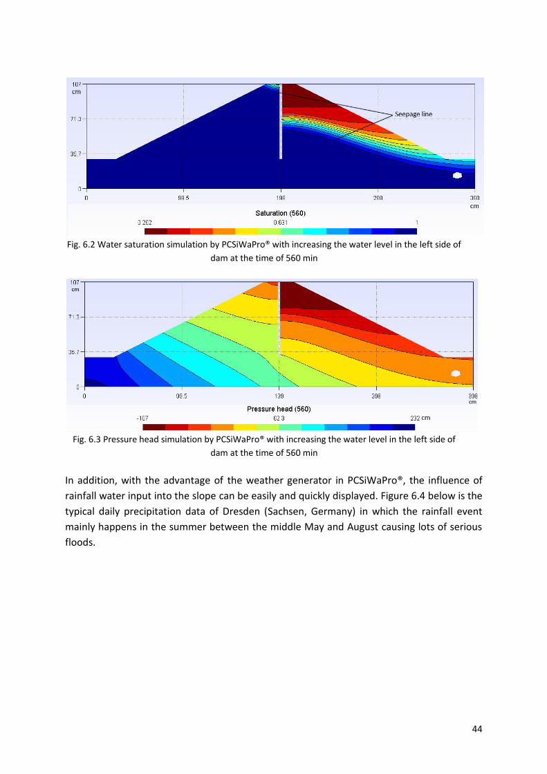
44

Fig. 6.2 Water saturation simulation by PCSiWaPro® with increasing the water level in the left side of

dam at the time of 560 min

Fig. 6.3 Pressure head simulation by PCSiWaPro® with increasing the water level in the left side of

dam at the time of 560 min

In addition, with the advantage of the weather generator in PCSiWaPro®, the influence of

rainfall water input into the slope can be easily and quickly displayed. Figure 6.4 below is the

typical daily precipitation data of Dresden (Sachsen, Germany) in which the rainfall event

mainly happens in the summer between the middle May and August causing lots of serious

floods.

45

Fig. 6.4 Daily precipitation data of Dresden from the weather generator of PCSiWaPro®

With PCSiWaPro® a simulation of water saturation during the experiment has been exhibited

in Figure 6.5 for this physical dam without consideration of rainfall water infiltration into the

slope. Figures 6.6 and 6.7 represent the simulation results of water saturation and pressure

head distribution with input of the weather data information of 15th June from PCSiWaPro®.

Rainfall water provides an additional flow into the top part of the right dam embankment

which is covered by a permeable layer, thereby increasing water content and pressure head

in this unsaturated slope and causing more possibility of slope collapse. With the continuous

rainfall event, the red part (dry) of the left slope will be saturated.

Fig. 6.5 Water saturation distribution simulated by PCSiWaPro® in a physical earth dam without input of

rainfall water at the time of 360 min

0.00

0.50

1.00

1.50

2.00

2.50

3.00

3.50

4.00

Jan Feb Mar Apr May Jun Jul Aug Sep Oct Nov Dec

Dai

ly p

reci

pit

atio

n (

cm/d

)

Date

Daily precipitation

Precipitation

Seepage line

46

Fig. 6.6 Water content distribution simulated by PCSiWaPro® in a physical earth dam in a heavy rainfall

event at the time of 360 min

Fig. 6.7 Pressure head distribution simulated by PCSiWaPro® in a physical earth dam in a heavy rainfall

event at the time of 360

6.1.3 Sensitivity analysis of model parameters

The above discussed simulation was mainly based on the existing data of hydraulic soil

parameters (like van Genuchten parameters, porosity) and the geometry (like slope angle)

which could be directly obtained from the laboratory test; however in the real practices

especially before the new construction of a hydraulic structure, it is essential for the civil

engineers and geoscience engineers to implement some sensitivity analysis for those

different parameters within the simulation work to study how greatly they influence the

hydrological process in the hydraulic structure and then the stability. For this purpose, an

example of sensitivity analysis is complied with the variable values of a van Genuchten

parameter α and the other parameters are kept as constants.

Seepage line

47

Fig. 6.8 Water saturation distribution simulated by PCSiWaPro® in a physical earth dam with the van

Genuchten parameters α = 1 m-1, n = 1.9 at the time of 240

Fig. 6.9 Water saturation distribution simulated by PCSiWaPro® in a physical earth dam with the van

Genuchten parameters α = 2 m-1, n = 1.9 at the time of 800 min

Figures 6.8 and 6.9 above represent the results of water saturation distribution at the same

simulation time with a constant water level of 30 cm at the left side of the physical dam.

Although the seepage lines convey no clear change when the value of the van Genuchten

parameter α increases by a factor of two (from 1 m-1 to 2 m-1), a significant difference can be

discovered in the partially saturated zones above the seepage line especially in the top part

of the dam body. Then by this fact an easy conclusion can be achieved that the van

Genuchten parameter α provides a large contribution to the unsaturated water distribution;

i.e. the larger value of the parameter α of the soil material results in the lower saturation or

water content distribution in those unsaturated zones.

48

6.2 Simulation for a Chinese earth dam

6.2.1 Site description

A real earth dam has been investigated in China for the practical application of the program

PCSiWaPro® and then for the slope stability analysis. This dam has 600 m width and 86 m

height. Additional site data, i.e. precipitation, water level change in the reservoir, pore water

pressure in the observation points, have been obtained from the local agencies. This earth

dam mainly contains three parts, two cores with slightly sandy clay (the bigger one is in the

middle and the smaller is closer to the left bottom) and silty sand in the remaining dam body

shown in Figure 6.10. As there are no available data for the van Genuchten parameters of

the soils, the estimated values have been applied from the program PCSiWaPro®. The

detailed estimated values have been shown below as

slight sandy clay-- θ = 0.01; θ = 0.52,α=0.084 (1/cm), n = 1.08, k = 9*10-7 m/s

silty sand-- θ = 0.01, θ = 0.38, α = 0.204 (1/cm), n = 1.23, k = 5*10-5 m/s

Fig. 6.10 Setup of soil materials in the Chinese earth dam in PCSiWaPro®

Figure 6.11 shows the precipitation data and water level change in the reservoir for 9

months of the year 2012. As can be seen in this graph, the rainfall event mainly occurred

between the middle of April and June, and in August. In addition, the water level in the

reservoir has exhibited a sharp decrease by 3 meters from the middle of March to the

middle of April, which was mainly due to the manmade pre-operation of outflow discharge

from the reservoir in order to prevent the possible overload water storage in the coming

rainfall season and to prevent the dam collapse. This pre-operation could be also obviously

found in later February and the middle of June. However, after early September a slow

49

decrease of water level has been detected in the reservoir, which could be explained by the

evaporation loss of water and very few rainfall events during this period.

Fig. 6.11 Precipitation and water level changes during the simulation period of 9 months in the reservoir

6.2.2 Hydrological simulation results

In the program PCSiWaPro®, an earth dam model has been set up with a simulation time of 9

months. On some part of the right slope of this model, atmospheric boundary condition has

been defined and for the rest of the right slope a boundary condition of seepage face is

given; the whole left slope is input by the boundary condition of no flux, which means no

water can pass through the impermeable slope; lastly the left foot of the dam has been

determined by a boundary condition of time dependent potential head due to the change of

water level in the reservoir (illustrated in Figure 6.12).

Fig. 6.12 Setup of boundary conditions for this Chinese earth dam

77.0

77.5

78.0

78.5

79.0

79.5

80.0

80.5

81.0

0.00

0.01

0.02

0.03

0.04

0.05

0.06

0.07

0.08

0.09

0.10

Jan Feb Mar Apr May Jun Jul Aug Sep

wat

er

leve

l in

th

e r

ese

rvio

r (m

)

dai

ly p

reci

pit

atio

n (

m/d

)

date

Precipitation (m/d) water level(m)

50

With the daily input data of precipitation and water level change, the daily variation of

pressure head, water content and saturation distribution can be easily achieved in this

Chinese earth dam. Figure 6.13 shows the simulation result of pressure head influenced by

both the groundwater variation and atmospheric condition on 29th June with a relatively dry

weather. The rigid decrease of seepage line in the clay cores can be explained by the fact

that the clay material has the smaller permeability than the silt sand in the slope.

Fig. 6.13 Pressure head simulation from PCSiWaPro® (182 is the simulation day time according to June

29th, 2012)

Figure 6.14 provides an image of water content distribution in the dam body on the same

day, especially in the unsaturated slope and clay core. In the saturated areas, the two clay

cores show higher saturated water content with a color of dark blue than the other part of

the dam, which is due to the different soil porosities; the higher the porosity is, the larger

the saturated soil water content will be. The zoom-in image in Figure 6.14 describes the

detailed distribution of water content from 9% to 40% near the seepage line in those

unsaturated zones; at the left side, circled by a black line, there is an interesting part in the

capillary fringe which exhibits a smaller degeneration rate of soil water in the core than that

in the slope with water level changing in the reservoir. This can offer a clear evidence for

sensitivity analysis of the model parameters (hydraulic conductivity, pore space diameter);

i.e. with the smaller hydraulic conductivity and smaller pore space diameter, the clay soil has

larger capillary force to hold the pore water, and then larger hysteresis effect on the water

content change. In addition, at the right side of the zoom-in image, some top part of the

middle clay core slope has been ‘eroded’ and saturated by the rainfall water infiltration

shown in dark blue.

51

#

Fig. 6.14 Water content simulation from PCSiWaPro® (182 is the simulation day time according to June

29th, 2012)

In Figure 6.15, water saturation distribution has been also simulated by PCSiWaPro® at the

same time. The highest water saturation with the light blue color in the unsaturated slope is

mainly due to the heavy rainfall event one week before 29th of June; then during the next

period of ten days, the upper layer of the slope suffered from the dry weather and became

drier, which is proved by the degradation of the soil water saturation from the deeper slope

to the subsurface layer shown in the zoom-in image of Figure 6.15. Moreover, in the zoom-in

image the width of the strip of infiltrated rainwater at the bottom of the unsaturated slope is

a little bit larger than on the top. In this case, the infiltrated rainfall water not only flows

perpendicular to the slope but also accumulates downward at the bottom (the zone circled

by a black line); in this reason, the rainfall water finally plays a small role in contributing to

the groundwater recharge. Lastly, in the zoom-in image the wiggles of seepage line is mainly

due to the large mesh of the model structure; when the mesh is getting finer, then a much

smoother seepage line can be obtained and the simulation results will be more accurate.

Seepage line

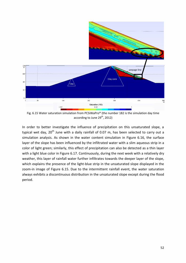
52

Fig. 6.15 Water saturation simulation from PCSiWaPro® (the number 182 is the simulation day time

according to June 29th, 2012)

In order to better investigate the influence of precipitation on this unsaturated slope, a

typical wet day, 20th June with a daily rainfall of 0.07 m, has been selected to carry out a

simulation analysis. As shown in the water content simulation in Figure 6.16, the surface

layer of the slope has been influenced by the infiltrated water with a slim aqueous strip in a

color of light green; similarly, this effect of precipitation can also be detected as a thin layer

with a light blue color in Figure 6.17. Continuously, during the next week with a relatively dry

weather, this layer of rainfall water further infiltrates towards the deeper layer of the slope,

which explains the presence of the light-blue strip in the unsaturated slope displayed in the

zoom-in image of Figure 6.15. Due to the intermittent rainfall event, the water saturation

always exhibits a discontinuous distribution in the unsaturated slope except during the flood

period.

seepage line

53

Fig. 6.16 Water content simulation from PCSiWaPro® within a wet weather (the number 173 is the

simulation day time according to June 20th, 2012)

Fig. 6.17 Water saturation simulation from PCSiWaPro® within a wet weather (the number 173 is the

simulation day time according to June 20th, 2012)

The detailed quantity of the influence of precipitation on the slope is shown in Figure 6.18

and Table 2 with a comparison between two small images representing the water content

Seepage line

Seepage line

54

distribution in different layers during the wet weather on 20th June and the dry weather on

29th June. The heavy rainfall event on 20th June increased the water content in the top

surface layer (0-1.5m) of the slope to 30%; then after ten days of evaporation, the top

surface got drier and reached a water content of only 14%. However in the deeper layer (>

1.5 m) there is no clear difference of water content having been detected in Figure 6.18

within the change of atmospheric conditions. In this case, it is concluded that water content

(or saturation) of the slope subsurface is much more sensitive to the atmospheric conditions

than that of the deeper layers, especially during a short period (e.g. ten days).

During the wet weather

During the dry weather

Fig. 6.18 Water content distribution in the unsaturated slope during the wet and dry weather

55

Table 2 Comparison of water content in the different layers during the wet and dry weather

Depth in the unsaturated slope (at air

side, m)

Water content θ in the different layers on two days

20.06.2012 29.06.2012

0.2 0.30 0.14

0.7 0.30 0.21

1.5 0.27 0.20

2 0.25 0.25

4 0.29 0.29

9 0.09 0.09

18 0.09 0.09

30 0.38 0.38

40 0.38 0.38

6.2.3 Comparison between the measured and simulated results

With the calibration system in PCSiWaPro®, a comparison can be carried out between the

measured and simulated water levels at the observation points whose positions are shown

in Figure 6.19. The groundwater levels have been measured every two weeks for nine

months by the piezometers set up in those two points.

Fig. 6.19 Position of the two observation points in the Chinese earth dam

The accordance between the measured and the computed results is good for an observation

point in the clay core illustrated in Figure 6.20. However some deviation is found in the

comparison of simulated and measured values for water level in the slope (Figure 6.21). This

is explained by the fact that our simulation was mainly based on the soil data base DIN 4220

and not on the exact soil parameter investigation in China. Last but not least, due to the

man-made operation of water level decrease in the reservoir from the middle of March to

the middle of April, both of the figures show a uniform decrease of water level during the

same period. And the relatively gentler decrease of water level in the clay core compared

with that in the slope can be also taken as a powerful proof for the validity of the sensitivity

analysis discussed before.

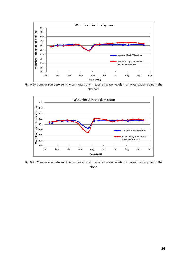
56

Fig. 6.20 Comparison between the computed and measured water levels in an observation point in the

clay core

Fig. 6.21 Comparison between the computed and measured water levels in an observation point in the

slope

292

293

294

295

296

297

298

299

300

301

302

Jan Feb Mar Apr May Jun Jul Aug Sep Oct

Wat

er

leve

l (ab

ove

th

e s

ea

leve

l) (

m)

Time (2012)

Water level in the clay core

caculated by PCSiWaPro

measured by pore water pressure measurer

297

298

299

300

301

302

303

304

305

Jan Feb Mar Apr May Jun Jul Aug Sep Oct

Wat

er

leve

l (ab

ove

th

e s

ea

leve

l) (

m)

Time (2012)

Water level in the dam slope

caculated by PCSiWaPro

measured by pore water pressure measurer

57

6.3 Simulation for a dump slope of a mining pit

Mining activities are always essential for the production of necessary minerals and then for

the development of modern society. However they also cause lots of serious environmental

and ecological problems, among which the dump slope landslide in the mining pit is one of

the main concerns. Constantly appearing causes have a great weight on the issue of

slope stability, like heavy rainfall events and ground water flow. Figure 6.22 shows a basic

structure for an unsaturated dump slope in a mining area, which displays the various factors

affecting the water balance and then the stability, e.g. structure geometry, vegetation,

precipitation, groundwater flow.

Fig. 6.22 A simplified structure of a dump site (System Analysis Group)

6.3.1 Site description

This study area locates between Leipzig and Bitterfeld in the city center of Delitzsch which

has been shaped by the lignite mining activities for more than one century as shown in

Figure 6.23.

Fig. 6.23 Location of this study area (Brueckner et al., 2013)

58

A real dump slope model has been selected from this mining area for the practical

application of the program PCSiWaPro® and then for stability analysis. This slope structure is

totally 300 meters wide and 11 meters high with sandy horizontal layers, sandy slope and 20

meters depth of clay layer shown in Figure 6.24. Additional basic data, like soil hydraulic

conductivities and records of groundwater water level change, have been obtained from the

local agency and the company IBGW Leipzig. The van Genuchten parameter values of the

different soils have been easily estimated in the program PCSiWaPro®. The detailed values

have been shown below as

clay -- k =10-8m/s, = 0.01, = 0.52, α = 0.066(1/cm), n = 1.1

sandy soil 1-- k=1.3*10-5m/s, = 0.01, = 0.4, α = 0.01(1/cm, assumed), n = 2 (assumed)

sandy soil 2 -- k = 5.2*10-4m/s, = 0.01, = 0.4, α = 0.01(1/cm, assumed), n = 2 (assumed)

sandy soil 3 -- k = 10-4m/s, = 0.01, = 0.4, α = 0.01(1/cm, assumed), n = 2 (assumed)

sand soil 4 -- k = 4.5*10-5m/s, =0.01; θ =0.4, α = 0.264(1/cm), n = 1.35

Fig. 6.24 Structure of a dump slope generated by PCSiWaPro® with clay soil and different sandy soils

6.3.2 Hydrological simulation results

After setup of the model in the program PCSiWaPro®, a simulation period of five years from

January 2000 to December 2004 was selected. On the dump slope, atmospheric boundary

condition was defined, which meant this slope received input of rainfall water; after the

formation of this dump slope, a constant groundwater level of 88 m was detected during

this simulation period, which supported the determination of the boundary condition of

constant potential head on the left side of this model.

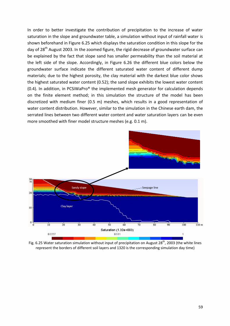
59

In order to better investigate the contribution of precipitation to the increase of water

saturation in the slope and groundwater table, a simulation without input of rainfall water is

shown beforehand in Figure 6.25 which displays the saturation condition in this slope for the

day of 28th August 2003. In the zoomed figure, the rigid decrease of groundwater surface can

be explained by the fact that slope sand has smaller permeability than the soil material at

the left side of the slope. Accordingly, in Figure 6.26 the different blue colors below the

groundwater surface indicate the different saturated water content of different dump

materials; due to the highest porosity, the clay material with the darkest blue color shows

the highest saturated water content (0.52); the sand slope exhibits the lowest water content

(0.4). In addition, in PCSiWaPro® the implemented mesh generator for calculation depends

on the finite element method; in this simulation the structure of the model has been

discretized with medium finer (0.5 m) meshes, which results in a good representation of

water content distribution. However, similar to the simulation in the Chinese earth dam, the

serrated lines between two different water content and water saturation layers can be even

more smoothed with finer model structure meshes (e.g. 0.1 m).

Fig. 6.25 Water saturation simulation without input of precipitation on August 28th, 2003 (the white lines

represent the borders of different soil layers and 1320 is the corresponding simulation day time)

Seepage line

60

Fig. 6.26 Water content simulation results without input of precipitation on August 28th, 2003 (the

number 1320 is the corresponding simulation day time)

Figure 6.27 exhibits the precipitation data output from the weather generator in

PCSiWaPro® for a typical year in the region of Leipzig. As can be seen in this graph, the

rainfall events mainly occur in the summer between June and September, especially in the

mid-June, early July and early September. In addition, although the rainfall season came

every year from mid-June, the groundwater level showed no change between the year of

2000 and 2004, which was mainly due to the manmade operation of pumping discharge

from the groundwater during the mining activities in order to prevent the possible overload

in groundwater storage especially in the rainfall season and to prevent the possible

geological and environmental disasters.

Fig. 6.27 Typical precipitation data for one year in Leipzig from the weather generator in PCSiWaPro®

Making use of the weather generator, the effect of rain water was included into the

simulation for the sandy slope which had the atmospheric boundary condition. The result of

water saturation distribution is illustrated in Figures 6.28, 6.29 and 6.30. Figure 6.28

represents the simulation for 30th April 2003; during the first four months, the weather was

relatively dry compared with that in the summer which caused low water saturation in this

sandy slope. However, in Figure 6.29 the clear increase of water saturation has been

expressed due to the rainfall on 28th August. Rainfall water provided an additional flow into

0

0.005

0.01

0.015

0.02

0.025

0.03

0.035

0.04

Jan Feb Mar Apr May Jun Jul Aug Sep Oct Nov Dec

Pre

cip

itat

ion

(m

/d)

Time(d)

Precipitation

Precipitation

Seepage line

61

some part of the top and the right sand slope embankment, thereby increasing water

content in this unsaturated slope. The highest water saturation was found to be 70%; in

addition, the rainfall water reaching the groundwater table in the slope performed

complementary to the groundwater recharge. Furthermore, with more rainfall in the next

month (September), the rain water continuously infiltrated into the slope and the soil water

from the rainfall in July has been also detected to flow deeper into the slope shown in Figure

6.30. The interspaces between the two light green water layers are mainly resulted from the

gap between the rainfall events. From these simulations, the dynamic influence of rainfall

water on the variation of water saturation in the unsaturated slope is exhibited and can be

easily understood.

Fig. 6.28 Simulation of water saturation distribution with input of precipitation on April 30th, 2003 (1200 is

the corresponding simulation day time in the program)

Fig. 6.29 Simulation of water saturation distribution with input of precipitation on August 28th, 2003

(1320 is the corresponding simulation day time in the program)

Seepage line

Seepage line

62

Fig. 6.30 Simulation of water saturation distribution with input of precipitation on September 17th, 2003

(1340 is the corresponding simulation day time in the program)

6.3.3 Comparison between the measured and simulated results

Due to the constant groundwater table after the year 2000, a stable value was achieved for

the water level measurement from an observation well in this dump slope. A comparison

between the measured and simulated water level has been carried out in Figure 6.31. The

accordance between the measured and the computed values using the program PCSiWaPro®

was good for our study area. However, only a little bit of deviation found in the comparison

could be explained by the fact that our simulation was mainly based on the average values of

those different dump soil parameters (e.g. average porosity, hydraulic conductivity);

however, the accuracy of the simulation can be improved with more field and laboratory

investigation for soil parameters of the different dump slope soils.

Fig. 6.31 Comparison between the simulation data and the measurement data in the observation well

6.4 Conclusion

1) The simulation results for the physical dam model in the laboratory indicated clearly

that ground water flow had been already detected in the highly saturated dam body;

and due to the increasing water saturation, the stability of this unsaturated slope was

influenced with an already happening surficial landslide.

0

20

40

60

80

100

2001 2002 2003 2004 2005

Gro

un

dw

ate

r le

vel a

bo

ve t

he

se

a le

vel (

m)

Year

calculated values

measured values

Seepage line

63

2) With the program PCSiWaPro®, water content and saturation distribution in the slope

zone can be simulated and predicted dynamically within the whole study period, which

is the preliminary work for stability analysis by the infinite slope model.

3) These studies have also shown the ability of PCSiWaPro® to simulate the groundwater

level variation in observation wells within a continuous period.

4) The agreement between the measured groundwater level and the computed one using

the program PCSiWaPro® was good for our real study areas (the Chinese earth dam and

the dump slope of the mining pit); however there was a little deviation between those

two values, especially in the Chinese earth dam slope. These deviations could be caused

by poorly estimated soil parameters (e.g. porosity, hydraulic conductivity) which were

based on the given DIN 4220 values. In this case, more investigation work for those soil

parameters in both the field and the laboratory is needed in order to get better

matching between the PCSiWaPro® simulation and real observation.

64

CHAPTER 7 Discussion of stability analysis results

7.1 Infinite slope analysis for the surficial landslide

In Chapter 5, the typical infinite slope analysis model (equation 24) has been put forward as

shown below

β

γ β

γ

θ θ

θ θ

β β

However with the equations 12, 13 and 18 expressing the relationships between the soil

water content and soil properties (cohesion, matric suction and internal friction angle), this

infinite slope model can be improved with the additional consideration of water content in

the unsaturated slope. Then based on the simulation results from the program PCSiWaPro®,

three scenarios of stability analysis from different sites are carried out by the improved

infinite slope model.

7.1.1 Infinite slope analysis for the Chinese earth dam

Figure 7.1 shows the simulation of the water content distribution by PCSiWaPro® in the

Chinese earth dam on 29.06.2012, a typical dry day. At the air side of the dam in the

unsaturated slope, one part (Figure 7.2) is selected for stability analysis within eight layers of

different water contents and different depths.

Fig. 7.1 Water content distribution simulated by PCSiWaPro® in the Chinese earth dam on 29.06.2012

during a dry weather (182 is the corresponding simulation day time in the program)

Seepage line

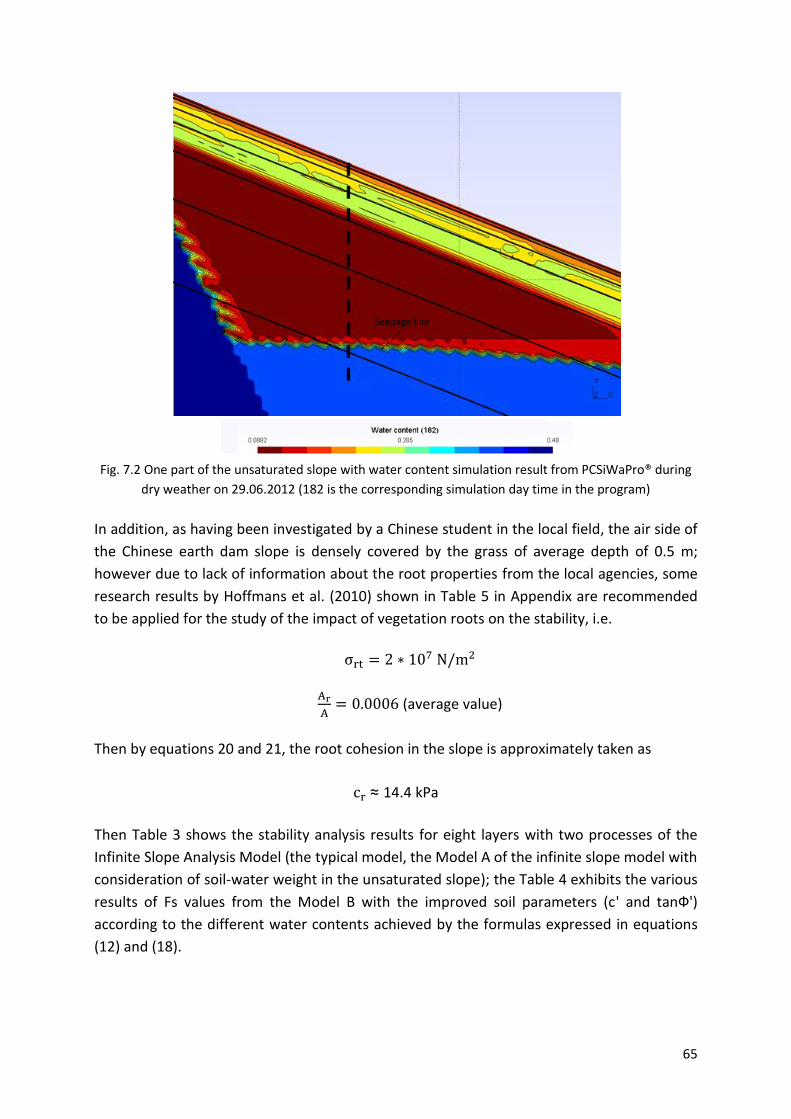
65

Fig. 7.2 One part of the unsaturated slope with water content simulation result from PCSiWaPro® during

dry weather on 29.06.2012 (182 is the corresponding simulation day time in the program)

In addition, as having been investigated by a Chinese student in the local field, the air side of

the Chinese earth dam slope is densely covered by the grass of average depth of 0.5 m;

however due to lack of information about the root properties from the local agencies, some

research results by Hoffmans et al. (2010) shown in Table 5 in Appendix are recommended

to be applied for the study of the impact of vegetation roots on the stability, i.e.

(average value)

Then by equations 20 and 21, the root cohesion in the slope is approximately taken as

≈ 14.4 kPa

Then Table 3 shows the stability analysis results for eight layers with two processes of the

Infinite Slope Analysis Model (the typical model, the Model A of the infinite slope model with

consideration of soil-water weight in the unsaturated slope); the Table 4 exhibits the various

results of Fs values from the Model B with the improved soil parameters (c' and tanФ')

according to the different water contents achieved by the formulas expressed in equations

(12) and (18).

Seepage line

66

On the first layer, 0.2 m, with water content of 14% and vegetation root system, the typical

infinite slope model shows a very safe value, 76.5; while with an assumption of no root

system on this layer, a much smaller Fs value, 62.6, is achieved from this model. This clearly

verifies the significant positive effect of vegetation on the stability. In addition, the typical

infinite slope model has been always applied without consideration of the soil water in the

slope, resulting in the overestimation of the stability especially during the rainfall event,

which can be proved by a comparison between the Fs value of 76.5 (from the typical infinite

slope model) and the Fs value of 70.0 (from the Model A with consideration of soil-water

weight). This overestimation is also confirmed by the stability analysis in other slope layers

with different water content and is significantly obvious in the subsurface layers; however,

for the deeper layers of the slope, the influence of water weight on the stability can be

neglected; as on the two deepest layers of 30 m and 40 m with the saturated water content,

the Fs values given by the typical infinite slope model and model A exhibit no clear

difference. Furthermore, in order to study how water content can affect stability, an

assumed water content value (3%) is selected for the subsurface layer of 0.2 m. This leads to

a higher Fs value (>100) obtained by model A, which clearly indicates the negative influence

of water content on the stability of the earth slope; the higher water content in the slope is

followed by less stability.

Table 3 Fs results from the infinite slope model

Depth in the slope* (at air

side, m)

Water content θ

Saturation (%)

Ua-Uw (kPa)

Fs value from the typical infinite slope model

Fs value from the infinite slope model with

consideration of soil water weight (Model A)

0.2 0.14 37 46.1 76.5 70.0

0.2** 0.14 37 46.1 62.6 57.0

0.2*** 0.03 8 1.5*105 >100 >100

0.7 0.21 55 6.9 16.6 15.3

2 0.25 66 3.0 6.8 6.2

4 0.29 76 1.3 4.2 3.9

9 0.09 24 382.0 4.2 3.9

18 0.09 24 382.0 3.0 2.8

30 0.38 (saturated)

100 0 1.68 1.67

40 0.38 (saturated)

100 0 1.67 1.66

Silt sand: c’s = 13.1 kPa; c’0 = 51.1 kPa; Ф‘s = 32°; Ф‘0 = 35°; γsoil = 1.415 g/cm3; θ = 0.01; θ = 0.38

Slope angle = 1 / 2.5

* vegetation root depth = 0.5 m

** no vegetation layer (an assumption)

*** assumption with different water content in the layer of 0.2 m

typical model

β

γ β

γ

θ θ

θ θ

β β

Model A

β

γ

β

γ

θ θ

θ θ

β β

Both models have constant cohesion and internal friction angle.

67

Last but not least, when Model B is applied for the stability analysis in this slope, even

smaller Fs values are obtained, e.g. the Fs value of 66.0 at the water content of 0.14 in the

layer of 0.2 m, nearly 9 less than that from the typical model and 4 less than that from the

improved Model A. This phenomenon can also be detected in other layers and it can be

concluded that the influence of water content on the soil parameters (c' and Ф') infers a

significant negative effect on the stability. However, for the deeper layers (i.e. deeper than 9

m) of this Chinese earth dam slope, there is no clear difference being detected between the

Fs values from Model B and that from the other two models, which means that the influence

of water content is negligible in the stability analysis for the deep slope of this study site.

Table 4 Fs values with the improved soil parameters’ values due to the water content change

Depth in the slope* (at air

side, m)

Water content θ

Saturation (%)

improved c' (kPa)

improved tanφ'

Fs value from the infinite slope model

with the improved soil parameters, c' and φ'

(Model B)

0.2 0.14 37 46.9 0.67 66.0

0.2** 0.14 37 46.9 0.67 54.2

0.2*** 0.03 8 50.5 0.70 >100

0.7 0.21 55 44.0 0.66 13.4

2 0.25 66 42.5 0.65 5.3

4 0.29 76 39.4 0.64 3.2

9 0.09 24 48.7 0.68 3.8

18 0.09 24 48.7 0.68 2.8

30 0.38 (saturated)

100 20.0 0.62 1.67

40 0.38 (saturated)

100 20.0 0.62 1.66

Silt sand: c’s = 13.1 kPa; c’0 = 51.1 kPa; Ф‘s = 32°; Ф‘0 = 35°; γsoil = 1.415 g/cm3; θ = 0.01; θ = 0.38

Slope angle = 1 / 2.5

As in Chapter 6, precipitation plays a significant role to increase the water content especially

in the subsurface layer (0 - 1.5 m) of the unsaturated slope. Based on the results from Table

4, the contribution to water content increase from precipitation provides a negative

influence on slope stability. In order to study how detailed precipitation affects the stability,

a simulation result for the unsaturated slope on 20.06.2012 with typical wet weather is given

as an example in Figure 7.3; due to the infiltrated rainfall water in this unsaturated slope, the

* vegetation root depth = 0.5 m

** no vegetation layer (an assumption)

*** assumption with different water content in the layer of 0.2 m

Model B

β

γ

β

γ

θ θ

θ θ

β β

–

= tan (

)

68

subsurface layer expresses the highest water content (0.3) with a color of light green which

is more than two times the water content in the subsurface shown in Figure 7.2.

Furthermore, under this layer there is no clear difference in water content between dry and

wet atmospheric conditions. Table 5 expresses the final results for Fs values for the slope

from Model A which exhibits a unified decrease due to the additional rainfall infiltration in

the subsurface layer as compared to Table 3; for example, when the water content at the

depth of 0.2 m increases from 0.14 shown in Table 3 to 0.3 in Table 5, the Fs value from

Model A correspondingly decreases from 70 to 55.2. This result can be taken as an obvious

proof for the negative contribution of precipitation on slope stability. However in the layers

deeper than 2 m the Fs values show no clear difference between both weather conditions.

The stability of the subsurface slope layer (instead of that in the deep layer) is therefore

much more sensitive to precipitation than that of the deep slope layer.

Fig. 7.3 One part of the unsaturated slope with water content simulation result from PCSiWaPro® during

wet weather (the number 173 is the corresponding simulation day time on June 20th, 2012)

Seepage line

69

Table 5 Fs results from the original infinite slope model and the improved Model A

Depth in the slope* (at air side,

m)

Water content θ

Saturation (%)

Ua-Uw (kPa)

Fs value from the infinite slope model with consideration of soil

water weight (Model A)

0.2 0.30 79 1.1 55.2

0.2** 0.30 79 1.1 43.5

0.2*** 0.38 100 0 52.4

0.7 0.30 79 1.1 13.6

0.7*** 0.38 100 0 13.1

2 0.25 66 3.0 6.1

4 0.29 76 1.3 3.9

9 0.09 24 382.0 3.9

18 0.09 24 382.0 2.8

30 0.38 (saturated)

100 0 1.67

40 0.38 (saturated)

100 0 1.66

Silt sand: c’s = 13.1 kPa; c’0 = 51.1 kPa; Ф's = 32°; Ф'0 = 35°; γsoil = 1.415 g/cm3; θ = 0.01; θ = 0.38

Slope angle = 1 / 2.5

Table 6 contains the Fs analysis results from Model B of the infinite slope model for this wet

earth dam slope. By comparison with Table 5, the same conclusions as found in the stability

analysis for the dry slope are also clearly displayed here, i.e. the higher water content is

followed by the lower Fs value, while the influence of water content on the stability for the

deep slope layers can be neglected.

* vegetation root depth = 0.5 m

** no vegetation layer (an assumption)

*** Assumption of water content of 0.38 in the layer

Model A

β

γ

β

γ

θ θ

θ θ

β β

Constant cohesion and internal friction angle

70

Table 6 Fs values from the Model B (with improved soil parameters’ values)

Depth in the slope* (at air

side, m)

Water content θ

Saturation (%)

improved c' (kPa)

improved tanφ'

Fs value from the infinite slope model

with the improved soil parameters, c' and φ'

(Model B)

0.2 0.30 79 38.7 0.64 44.98

0.2** 0.30 79 38.7 0.64 33.3

0.2*** 0.38 100 20.0 0.62 28.2

0.7 0.30 79 38.7 0.64 10.6

0.7*** 0.38 100 20.0 0.62 6.0

2 0.25 66 42.5 0.65 5.2

4 0.29 76 39.4 0.64 3.2

9 0.09 24 48.7 0.68 3.8

18 0.09 24 48.7 0.68 2.8

30 0.38 (saturated)

100 20.0 0.62 1.67

40 0.38 (saturated)

100 20.0 0.62 1.66

Silt sand: c’s = 13.1 kPa; c’0 = 51.1 kPa; Ф's = 32°; Ф'0 = 35°; γsoil = 1.415 g/cm

3; θ = 0.01; θ = 0.38

Slope angle = 1 / 2.5

In both stability analysis cases discussed above (the Chinese earth dam slope under the dry

and wet conditions), the additional consideration of soil water weight in the unsaturated

slope has resulted in the decrease of the Fs values; and the negative effects of water content

on the soil parameters (cohesion and internal friction angle) have further reduced the

stability especially in the subsurface layers. Moreover, the higher the change in the water

content in the subsurface layer is, the larger the difference between the Fs values from the

improved Model A and Model B will be.

According to the reference stability values from Bowels (1988) displayed in Table 1, this

Chinese earth dam slope has been confirmed to be stable under the both atmospheric

conditions; as the Fs values in Tables 3 and 5 are all larger than the minimum Fs value 1.6 for

the earth slope; however necessary prevention work is also in great need to reduce the risk

of landslides in the deep layers.

* vegetation root depth = 0.5 m

** no vegetation layer (an assumption)

*** Assumption of water content of 0.38 in the layer

Model B

β

γ

β

γ

θ θ

θ θ

β β

–

= tan (

)

71

7.1.2 Infinite slope analysis for the dump slope

Similarly, in the dump slope the infinite slope model is also expected to be applicable for the

stability analysis. For the calculation of Fs values, water saturation in the unsaturated slope

during dry weather on April 30th, 2003 has been simulated by PCSiWaPro® in Figure 7.4 and

further a zoom-in describing the study area is selected and displayed in Figure 7.5.

Fig. 7.4 Simulation of water saturation in the dump slope for dry weather on 30th April, 2003 (the number

1200 is the corresponding simulation day time in the program)

Fig. 7.5 A selected part from the unsaturated sandy slope for the stability analysis

Table 7 summarizes the stability analysis results for the selected five layers from the typical

infinite slope model and the improved Model A with consideration of soil-water weight in

this dump slope. In the first layer of 0.5 m depth with three water contents (one real data

0.17, two assumed values 0.02 and 0.39), the improved model A clearly displays the negative

influence of water content on the slope stability, as the higher water content value

corresponds to the lower Fs values. In addition, in the deep slope (e.g. the layer at the depth

of 8 m), the Fs values from those two models show no clear difference and the influence of

water content on the slope stability disappears, which means that the influence of soil water

Seepage line

Seepage line

72

weight in the infinite slope analysis is negligible for the deep slope. Both the conclusions

have been already confirmed in the analysis of the Chinese earth dam slope.

Table 8 exhibits the stability analysis results from the improved Model B with the additional

consideration of variable soil parameters due to the water content change. From these

results, a common phenomenon is achieved, i.e. Fs values have further decreased due to the

water content; for example, the subsurface layer 0.5 m with the saturated water content

(assumed) has been provided with a safe Fs value of 5.5 which is only 25% of the Fs value

from the improved model A and 20% of that from the typical model. Furthermore, on the

deeper layer (e.g. 8 m depth) there is no clear change of Fs value being found compared with

that from the other two models, which proves the same conclusion from the stability

analysis in the Chinese earth dam that the influence of water content on the variation of soil

parameters can be negligible for the stability analysis in the deep slope.

Table 7 Fs results from the typical infinite slope model and improved Model A

Depth in the slope* (at air

side, m)

Water content

θ

Saturation (%)

Ua-Uw (kPa)

Fs value from the typical

infinite slope model

Fs value from the infinite slope model with

consideration of soil water weight (Model A)

0.5 0.17 43 4.4 29.9 27.7

0.5* 0.02 5 1.2*104 >100 >100

0.5** 0.39 100 0 28.3 23.9

2 0.17 43 4.4 12.8 12.2

2** 0.39 100 0 12.4 11.3

4 0.17 43 4.4 9.8 9.6

5.5 0.17 43 4.4 9.2 8.9

8 0.39 100 0 5.5 5.5 Dump sand: c’s = 0 kPa; c’0 = 16.6 kPa; Ф's = 30°; Ф'0 = 36.5°; γsoil = 1.52 g/cm

3; θ = 0.01; θ = 0.39

Slope angle: tanβ = 0.105

* Assumption of water content of 0.02 in the layer ** Assumption of water content of 0.39 in the layer

typical model

β

γ β

γ

θ θ

θ θ

β β

Model A

β

γ

β

γ

θ θ

θ θ

β β

Both two models have constant cohesion and internal friction angle.

73

Table 8 Fs values from the improved Model B (with improved soil parameter values)

Depth in the slope* (at air

side, m)

Water content

θ

Saturation (%)

improved c' (kPa)

improved tanφ'

Fs value from the infinite slope model

with the improved soil parameters, c' and φ'

(Model B)

0.5 0.17 43 13.8 0.68 23.8

0.5* 0.02 5 16.50 0.73 >100

0.5** 0.39 100 0.00 0.58 5.5

2 0.17 43 13.8 0.68 10.8

2** 0.39 100 0.00 0.58 5.5

4 0.17 43 13.8 0.68 8.7

5.5 0.17 43 13.8 0.68 8.1

8 0.39 100 0.00 0.58 5.5 Dump sand: c’s = 0 kPa; c’0 = 16.6 kPa; Ф's = 30°; Ф'0 = 36.5°; γsoil = 1.52 g/cm

3; θ = 0.01; θ = 0.39

Slope angle: tanβ = 0.105 * Assumption of water content of 0.02 in the layer ** Assumption of water content of 0.39 in the layer

Model B

β

γ

β

γ

θ θ

θ θ

β β

–

= tan (

)

In addition, for the purpose of the study on the influence of precipitation, the water

saturation simulation result for 30th July, 2003 was applied to the infinite slope analysis. The

water saturation in this dump slope is shown in Figure 7.6 and the selected layer for the

stability analysis is found in Figure 7.7.

Fig. 7.6 Simulation of water saturation in the dump slope on a wet weather on 30th July, 2003 (1320 is the

corresponding simulation day time in the program)

Seepage line

74

Fig. 7.7 A selected part from the unsaturated sandy slope for the stability analysis

Tables 9, 10 contain the stability analysis results for this dump slope based on the infinite

slope analysis model. Comparing the Fs values for the same layers under different

atmospheric conditions, the increased water content in the subsurface layers due to the

rainfall infiltration has resulted in the decrease of the slope stability; for example, in the

layer of 0.5 m depth, the higher water content (0.24) has caused the decrease of the Fs

values by Models A and B when the influence of water content on slope stability is

considered. However, due to the low sensitivity on the water content in the deeper layers,

the Fs values of these layers exhibit no clear change, which is similar to the stability analysis

for the Chinese earth dam slope.

Table 9 Fs results from the typical infinite slope model and improved Model A

Depth in the slope* (at air

side, m)

Water content

θ

Saturation (%)

Ua-Uw (kPa)

Fs value from the typical

infinite slope model

Fs value from the infinite slope model with

consideration of soil water weight (Model A)

0.5 0.24 60 1.4 29.1 26.1

2 0.24 60 1.4 12.6 11.9

4 0.17 43 4.4 9.9 9.6

5.5 0.17 43 4.4 9.2 8.9

8 0.39 100 0 5.5 5.5 Dump sand: c’s = 0 kPa; c’0 = 16.6 kPa; Ф's = 30°; Ф'0 = 36.5°; γsoil = 1.52 g/cm

3; θ = 0.01; θ = 0.39

Slope angle: tanβ = 0.105

typical model

β

γ β

γ

θ θ

θ θ

β β

Model A

β

γ

β

γ

θ θ

θ θ

β β

Both models have constant cohesion and internal friction angle.

Seepage line

75

Table 10 Fs values from the improved Model B (with improved soil parameter values)

Depth in the slope* (at air

side, m)

Water content

θ

Saturation (%)

improved c' (kPa)

improved tanφ'

Fs value from the infinite slope model

with the improved soil parameters, c' and φ'

(Model B)

0.5 0.24 60 12.2 0.64 20.2

2 0.24 60 12.2 0.64 9.6

4 0.17 43 13.8 0.68 8.6

5.5 0.17 43 13.8 0.68 8.0

8 0.39 100 0.00 0.58 5.5 Dump sand: c’s = 0 kPa; c’0 = 16.6 kPa; Ф's = 30°; Ф'0 = 36.5°; γsoil = 1.52 g/cm

3; θ = 0.01; θ = 0.39

Slope angle: tanβ = 0.105

Model B

β

γ

β

γ

θ θ

θ θ

β β

–

= tan (

)

From the above stability analysis, quite similar to stability analysis for the Chinese earth dam,

it is easily concluded that the additional consideration of water content in the infinite slope

model has caused the decrease of Fs values especially for the subsurface layer of the dump

slope. Moreover, this slope exhibited relative large Fs values in all the five layers within the

eight meters depth, which declared the great stability of this dump slope and no necessary

prevention was needed.

7.1.3 Conclusions

1) Vegetation on the air side of dams and dikes has significant influence on the stability

of slopes from the root cohesion as well as water uptake by plant roots.

2) The influence of infiltrated rainfall in the unsaturated slope has been proved to be a

significant negative contribution to the slope stability.

3) The additional consideration of water content has resulted in a smaller Fs value when

applying the infinite slope model in the unsaturated slope (especially in the

subsurface layer and under the heavy rainfall event).

4) In the deeper layer of the slope under the saturated condition, the infinite slope

model told us that there was no clear difference between the Fs values for the

different depths.

5) By the infinite slope model, the Chinese earth dam and the dump slope have been

confirmed to be stable; however, for the deeper layer of the Chinese earth dam,

necessary prevention work was in great need to reduce the possible deep landslide.

6) Practically, with the water content simulation or prediction results (especially in the

heavy rainfall event) from the program PCSiWaPro®, the infinite slope stability model

can be taken as a powerful tool for forecasting the possible shallow surficial

76

landslides; combination of the program PCSiWaPro® and the infinite slope model can

also provide a basic guideline for the determination of the size and the structure (e.g.

the core and slope angle) of the safe earth dam.

7.2 Bishop’s Model analysis for the circular and deep landslide

As being discussed in Chapter 5, the limit equilibrium models like Bishop’s Model are

suitable for the forecasting of the circle slip landslide in the deeper layer of the earth dam

slope. However, the influence of the water content in the slope has been always neglected

during the application of those limit equilibrium methods, which can cause the

overestimation of the slope stability. In this case, the additional consideration of water

content will be included into the stability analysis in this section. The critical slip surface has

to be determined beforehand by the software GEO-SLOPE based on the simulation result of

the seepage line by the program PCSiWaPro®; then further with the simulation results of

water content in the whole slope from the program PCSiWaPro®, an improved stability

analysis will be carried out.

7.2.1 Stability analysis for the Chinese earth dam

7.2.1.1 Stability analysis by the GEO-SLOPE Software

The water content simulation result for a dry-weather day (29.06.2012) has been simulated

by PCSiWaPro® and expressed in Figure 7.8, which is a preparing work for the stability

analysis by the software GEO-SLOPE.

Fig. 7.8 Simulation result of water content in the Chinese earth dam on 29.06.2012 (182 is the

corresponding simulation day time in the program)

In the software GEO-SLOPE, the unsaturated soil parameters are usually used by the geo-

engineers to calculate the slope stability; in this reason, the values with the unsaturated

cohesion c’0 and the unsaturated internal friction angle Ф'0 shown below will be firstly

applied to our study site,

Silt sand: c'0 = 51.1 kPa; Ф'0 = 35°; γsoil = 1.415 g/cm3; θ = 0.01; θ = 0.38

Clay: c’0 = 102 kPa; Ф'0 = 28°; γsoil = 1.2 g/cm3; θ = 0.01; θ = 0.52

Seepage line

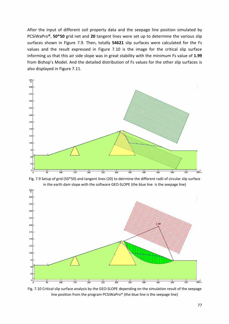
77

After the input of different soil property data and the seepage line position simulated by

PCSiWaPro®, 50*50 grid net and 20 tangent lines were set up to determine the various slip

surfaces shown in Figure 7.9. Then, totally 54621 slip surfaces were calculated for the Fs

values and the result expressed in Figure 7.10 is the image for the critical slip surface

informing us that this air side slope was in great stability with the minimum Fs value of 1.99

from Bishop’s Model. And the detailed distribution of Fs values for the other slip surfaces is

also displayed in Figure 7.11.

Fig. 7.9 Setup of grid (50*50) and tangent lines (20) to detrmine the different radii of circular slip surface

in the earth dam slope with the software GEO-SLOPE (the blue line is the seepage line)

Fig. 7.10 Critical slip surface analysis by the GEO-SLOPE depending on the simulation result of the seepage

line position from the program PCSiWaPro® (the blue line is the seepage line)

78

Fig. 7.11 Distribution map of Fs values for this Chinese earth dam with the minimum value in the center

(the blue line is the seepage line)

Within the software GEO-SLOPE, the determination of the slice increment number for

stability analysis depends on the precision required. In the stability analysis having been

already carried out, 31 slices (shown in Figure 7.12) were selected for the stability analysis

above the critical slip surface; in addition to the final Fs value, the force analysis for each

slice was also executed by the software GEO-SLOPE, and those force analysis data will be

taken as the basis for the next Fs improvement work.

79

Fig. 7.12 Division of the slope above the critical slip surface into 31 slices by GEO-SLOPE (the blue line is

the seepage line)

Two examples for the slice force analysis are given in Figures 7.13 and 7.14, one above the

groundwater table (the seepage line) and the other passed through by the groundwater

table, from which all the basic force data calculated by the software GEO-SLOPE can be

checked out like the slice base angle, slice weight, negative pore water pressure, slice width

and so on. For example, in Slice No. 4 which is above the seepage line, there is no influence

from the pore water pressure; while Slice No. 20 below the seepage line is associated with a

negative pore water pressure force of 307.8 kN/m. Those data can provide the geo-

engineers with an easy way for the stability analysis for each slice and for the purpose of the

slope structure design and protection. However, in these two figures the clear disadvantages

of this software can also be easily detected. As the fixed values of cohesion (51.1 kPa) and

internal friction angle (35°) for the unsaturated soil are applied to both the unsaturated Slice

No. 4 and the saturated Slice No. 20. The missing consideration of the influence of water

content on the variation of those two parameters has been discussed before and can result

in the overestimation of the final Fs value. In this case, the additional consideration of the

influence from water content on the variation of the soil parameters is greatly needed for a

better stability analysis result. In the next section, the sensitivity analysis of the soil

parameters related to the Fs value will be executed.

80

Fig. 7.13 Force analysis for the 4th slice above the seepage line (the unit for length is meter, the unit for

the force is Newton and the unit for the shear stress is Pascal)

Fig. 7.14 Force analysis for the 20th slice under the seepage line (the unit for the length is meter, the unit

for the force is Newton and the unit for stress is Pascal)

7.2.1.2 Sensitivity analysis of soil parameters in GEO-SLOPE

During the operation of the stability analysis by the software GEO-SLOPE, only three kinds of

parameter values were needed as input, i.e. the soil density, soil cohesion and internal

friction angle; the soil density is a constant value, while the other two parameters always

vary due to some factors like water content or compaction which has been proved by lots of

field and laboratory experiments. As being discussed in Chapter 5, the variation of cohesion

and internal friction angle has a close relationship with the change of the Fs values in the

slope stability analysis; in order to certify how detailed those parameters can influence the

final results of the Fs values, the sensitivity analysis of the soil parameters c’ and Ф’ for the

silt sandy slope are executed with the constant parameters for the clay core in the Chinese

earth dam in this section.

81

1) Sensitivity analysis for the cohesion (with a fixed internal friction angle Ф‘ = 35°)

Figure 7.15 and Table 11 are the sensitivity analysis results for soil cohesion based on a fixed

internal friction angle within the GEO-SLOPE software; it can be clearly detected that, with

fixed internal friction angle, the larger the soil cohesion is, the higher the Fs value of the

critical slip surface will be and this surface is located at lower depth. For example, when the

cohesion changes from the maximum value (51.1 kPa) to the minimum value (20 kPa), the Fs

value of the critical slip surface is accordingly decreased by 0.3.

c’ = 51.1 kPa c’ = 40 kPa

c’ = 30 kPa c’ = 20 kPa

Fig. 7.15 Sensitivity analysis for soil cohesion in the GEO-SLOPE software (the blue line is the seepage line)

82

Table 11 Sensitivity analysis of the soil cohesion in the GEO-SLOPE software with fixed Ф‘

Soil parameter Soil cohesion with a fixed internal friction angle Φ‘ = 35°

c’ = 51.1 kPa c’ = 38 kPa c’ = 30 kPa c’ = 20 kPa

Fs value of the critical slip surface (by Bishop’s model)

1.99 1.88 1.78 1.68

2) Sensitivity analysis of the internal friction angle (with a fixed cohesion c’ = 51.1 kPa)

As can be seen in Figure 7.16 and Table 12, the soil parameter Ф' also expresses a positive

relationship with the slope stability; the larger the internal friction angle is, the more stable

the slope will be.

Ф‘ = 35° Ф‘ = 34°

Ф‘ = 33° Ф‘ = 32°

Fig. 7.16 Sensitivity analysis for the internal friction angle with a fixed cohesion in the GEO-SLOPE software (the blue line is the seepage line)

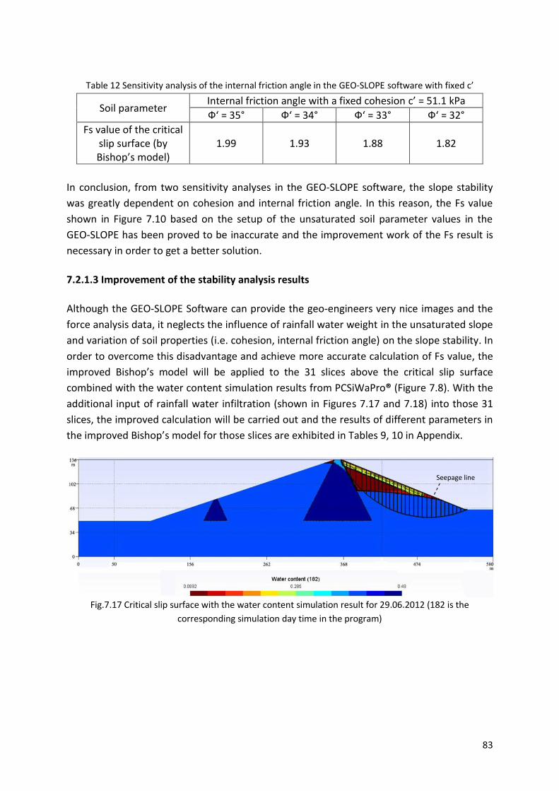
83

Table 12 Sensitivity analysis of the internal friction angle in the GEO-SLOPE software with fixed c’

Soil parameter Internal friction angle with a fixed cohesion c’ = 51.1 kPa

Ф‘ = 35° Ф‘ = 34° Ф‘ = 33° Ф‘ = 32°

Fs value of the critical slip surface (by Bishop’s model)

1.99 1.93 1.88 1.82

In conclusion, from two sensitivity analyses in the GEO-SLOPE software, the slope stability

was greatly dependent on cohesion and internal friction angle. In this reason, the Fs value

shown in Figure 7.10 based on the setup of the unsaturated soil parameter values in the

GEO-SLOPE has been proved to be inaccurate and the improvement work of the Fs result is

necessary in order to get a better solution.

7.2.1.3 Improvement of the stability analysis results

Although the GEO-SLOPE Software can provide the geo-engineers very nice images and the

force analysis data, it neglects the influence of rainfall water weight in the unsaturated slope

and variation of soil properties (i.e. cohesion, internal friction angle) on the slope stability. In

order to overcome this disadvantage and achieve more accurate calculation of Fs value, the

improved Bishop’s model will be applied to the 31 slices above the critical slip surface

combined with the water content simulation results from PCSiWaPro® (Figure 7.8). With the

additional input of rainfall water infiltration (shown in Figures 7.17 and 7.18) into those 31

slices, the improved calculation will be carried out and the results of different parameters in

the improved Bishop’s model for those slices are exhibited in Tables 9, 10 in Appendix.

Fig.7.17 Critical slip surface with the water content simulation result for 29.06.2012 (182 is the

corresponding simulation day time in the program)

Seepage line

84

Fig.7.18 Division of the unsaturated slope into 31 slices with the water content simulation result

An improved Fs is achieved as

Fs = 1.58

Compared with the Fs value of 1.99 calculated by the Software GEO-SLOPE exhibited in

Figures 7.10 and 7.11, a much smaller Fs value of 1.58 has been obtained from the improved

Bishop’s model with the additional consideration of soil water weight and the influence of

the water content on the variation of soil property parameters (cohesion and internal

friction angle) in the earth dam slope, which proves that the infiltrated rainfall water in the

unsaturated slope and the saturated soil water below the seepage line perform a significant

negative effect on the safety of the dam slope. This result can also be taken as a powerful

proof to certificate the overestimation of the slope stability carried out by the common

geotechnical calculation.

According to the minimum reference value for the stable earth slope in Table 1, the Chinese

earth dam slope has been examined to be close to instability; in this case, some necessary

prevention work is in great need to overcome the low Fs value and reduce the risk of slope

landslide; fortunately, on the right toe of this earth dam, a concrete structure layer has been

already set up for this purpose.

In the above mentioned stability analysis, the unsaturated soil parameter values (c’0 and Ф'0)

of the clay soil were used for the calculation of the critical slip surface position. From the

simulation result, most part of the clay soil was detected to be under the groundwater level

(i.e. under saturated condition); then those applied unsaturated soil parameters for the clay

could also easily lead to the overestimation of the Fs value.

Seepage line

85

In order to optimize this stability analysis, the ideal way is to set up the real soil parameter

values according to the different water content in the unsaturated slope and also in the

saturated dam body into the GEO-SLOPE software; however, this process is too complicated

to be achieved in the real practice especially for the quick decision support of landslide

forecasting in the flood period. In this reason, another sensitivity analysis of the soil

parameters (cohesion and internal friction angle) will be executed with the saturated

parameter values (c’s and Ф's shown below) in the GEO-SLOPE software for the stability

analysis in the same dump slope.

Silt sand: c’s =13.1 kPa; Ф's = 32°; γsoil = 1.415 g/cm3; θ = 0.01; θ = 0.38

Clay: c’s = 20 kPa; Ф's = 18°; γsoil = 1.2 g/cm3; θ = 0.01; θ = 0.52

With these saturated soil parameters, a much smaller Fs value (1.26) is provided by the GEO-

SLOPE software, and the result is expressed in Figure 7.19. Due to the low saturated

cohesion of the clay soil, the middle core is intersected by the critical slip surface. Above the

critical slip surface, the slope has been divided into total 35 slices (Figure 7.20) in order to

carry out the force analysis for each slice. Figure 7.21 shows the additional input of rainfall

water into the unsaturated slope.

Fig. 7.19 Stability analysis by the GEO-SLOPE with the input of the saturated soil parameters (the blue line

is the seepage line)

86

Fig. 7.20 Division of the critical slip surface into 35 slices (the blue line is the seepage line)

Fig. 7.21 Input of the influence of soil water into this earth slope (182 is the corresponding simulation day

time in the program)

As all those 35 slices are found to be below the seepage line, the definition of the saturated

soil parameters for both the clay and sand is proved to be applicable in this stability analysis

in the GEO-SLOPE Software. In addition, with the experience of the stability analysis from

Table 9 in Appendix, the contribution from the soil water weight can be neglected as

compared with the soil weight above the critical slip surface; based on these two reasons, it

is no longer needed to further improve the Fs value.

With the Fs calculation by the improved Bishop’s model, the range (1.26, 1.58) of the

improved Fs values under the definition of saturated and unsaturated conditions is achieved

as shown below (Figure 7.22); the closer the two values are, the more accurate this stability

analysis will be. The possible position of the critical slip surface is within the area between

the white borders; the possible minimum Fs value is within the range between the two

improved Fs values (1.26, 1.58).

Seepage line

87

Fig. 7.22 Definition of the possible position of the critical slip surface (area between the two white borders)

7.2.2 Bishop’s model analysis for the dump slope

7.2.2.1 Stability analysis by the GEO-SLOPE software

Within the dump slope, the combination of the program PCSiWaPro® and the software GEO-

SLOPE is also expected to be applicable for the stability analysis. Depending on the

simulation result from the Program PCSiWaPro® for the seepage line position in the sandy

dump slope shown in Figure 7.23, the critical slip surface can also be calculated by the

software GEO-SLOPE.

In practice, the unsaturated soil parameter values are always used as input for the GEO-

SLOPE software by the geo-engineers for the slope stability analysis; for our study site in the

dump slope, the unsaturated soil parameter values were firstly selected as shown below,

Dump sand: c'0 = 16.6 kPa; Ф'0 = 36.5°; γsoil = 1.52 g/cm3; θ = 0.01; θ = 0.39

Clay layer: c'0 = 95 kPa; Ф'0 = 28°; γsoil = 1.2 g/cm3; θ = 0.01; θ = 0.52

Seepage line

88

Fig. 7.23 Simulation of water saturation distribution with input of precipitation on August 28th, 2003

(1320 is the corresponding simulation day time in the program)

In the software GEO-SLOPE, after the input of different soil property data and the seepage

line position simulated by PCSiWaPro®, a 60*60 grid net and 50 tangent lines have been set

up to determine the various slip surfaces shown in Figure 7.24 and then totally 152561 slip

surfaces were selected for the calculation of different Fs values. The result in Figure 7.25 is

for the position of the critical slip surface and its Fs value (4.70) within the whole air side

slope which informs us that this dump slope is stable. In Figure 7.26 an overview of the Fs

value distribution is provided based on the fixed grid net and tangent lines.

Fig. 7.24 Setup of grids and tangent lines in the dump slope within the software GEO-SLOPE (the blue line

is the seepage line)

Seepage line

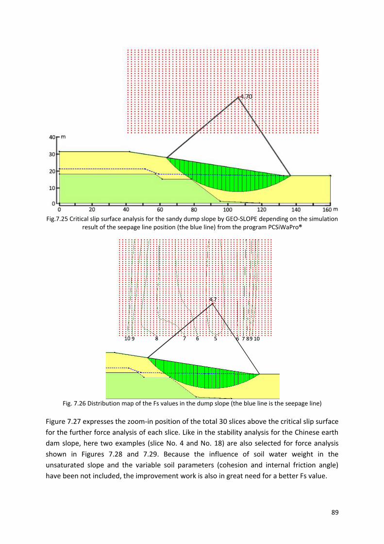
89

Fig.7.25 Critical slip surface analysis for the sandy dump slope by GEO-SLOPE depending on the simulation

result of the seepage line position (the blue line) from the program PCSiWaPro®

Fig. 7.26 Distribution map of the Fs values in the dump slope (the blue line is the seepage line)

Figure 7.27 expresses the zoom-in position of the total 30 slices above the critical slip surface

for the further force analysis of each slice. Like in the stability analysis for the Chinese earth

dam slope, here two examples (slice No. 4 and No. 18) are also selected for force analysis

shown in Figures 7.28 and 7.29. Because the influence of soil water weight in the

unsaturated slope and the variable soil parameters (cohesion and internal friction angle)

have been not included, the improvement work is also in great need for a better Fs value.

90

Fig. 7.27 Division of the slope above the critical slip surface into total 30 slices calculated from the

software GEO-SLOPE (the blue line is the seepage line)

Fig. 7.28 Force analysis for slice No. 4 above the groundwater table (the unit for length is meter, the unit

for force is Newton and the unit for shear stress is Pascal)

Fig. 7.29 Force analysis for slice No. 18 which is passed through by the groundwater table (the unit for the

length is meter, the unit for the force is Newton and the unit for the stress is Pascal)

91

7.2.2.2 Improvement of the stability analysis results

With the additional consideration of the influence of the water content in the slope on the

Fs value, the improved Bishop’s model is applied in this stability analysis. Figure 7.30 is the

water content distribution under the rainfall event on 30th July, 2003 with the input of the

calculation result for the critical slip surface.

Fig. 7.30 Analysis of slices above the critical slip with the consideration of soil water in the dump slope

(1320 is the corresponding simulation day time in the program)

In Tables 11, 12 in Appendix, besides the effect from the soil water in the unsaturated slope,

the contribution of water content to the variation of soil cohesion and internal friction angle

as shown in Table 13 is also included into the stability analysis. Finally, an improved Fs value

can be achieved as a safe value of 3.05, a much smaller factor compared with the Fs value of

4.70 without the consideration of water content in the slope shown in Figure 7.25. Due to

the influence of water content (including the saturated and unsaturated θ) on the variation

of the soil parameters and also the weight of rainfall water, the slope is found to be much

less safe than analyzed by GEO-SLOPE.

Table 13 Improved values of cohesion and internal friction angle for the dump sand

Soil parameters values at different water content

θ = 0.15/ Saturation=43%

θ = 0.39/ Saturation=100%

improved c' (kPa) 13.8 0

improved tanφ' 0.68 0.58

Furthermore, in order to separately analyze the contribution from the rainfall infiltration,

another stability analysis was carried out without the consideration of soil water weight in

the unsaturated slope. The stability factor increased to 3.17 (0.12 larger than the Fs value

from Tables 11, 12 in the appendix), from which the negative effect from the rainfall water

infiltration has been here clearly exhibited although the contribution is only little.

Seepage line

92

In order to increase the accuracy of the stability analysis result, similar to the stability

analysis for the Chinese earth dam slope, in this dump slope another sensitivity analysis with

the saturated soil property parameter values was executed.

In this calculation the following values were applied in the GEO-SLOPE software,

Dump sand: c’s = 0 kPa; Ф's = 30°; γsoil = 1.52 g/cm3; θ = 0.01; θ = 0.39

Clay layer: c’s = 20 kPa; Ф's = 18°; γsoil = 1.2 g/cm3; θ = 0.01; θ = 0.52

Then, similar to the stability analysis shown above, a new Fs value was obtained by the GEO-

SLOPE software based on saturated soil parameter values. The results are shown in Figure

7.31 with a much smaller value of 2.62 compared with the value of 4.7 from the unsaturated

soil parameters shown in Figure 7.25.

Fig. 7.31 Position of the critical slip surface and the distribution of the Fs values from the GEO-SLOPE

software (the blue line is the seepage line)

Figure 7.32 contains the analysis of all those 31 slices divided by the GEO-SLOPE software

from the area above the critical slip surface. Due to the saturated cohesion of the clay soil,

this critical slip surface also passes through the clay layer. When the rainfall water effect is

additionally included in the stability analysis, Figure 7.32 can be added in Figure 7.23, this

resulting in the combined effect as exhibited in Figure 7.33.

93

Fig. 7.32 Analysis of all those 31 slices above the critical slip surface (the blue line is the seepage line)

Fig. 7.33 Analysis of slices above the critical slip with the consideration of soil water in the dump slope

(1320 is the corresponding simulation day time in the program)

After all the preparation work has been done, a new stability analysis calculation can be

carried out and the details are illustrated in Tables 13, 14 in Appendix.

With the output calculation results from the GEO-SLOPE Software shown in Tables 13, 14 in

Appendix and the improved results of cohesion and internal friction angle expressed in Table

14 for the first four unsaturated sandy slices, an improved Fs result is achieved as

Fs = 2.80

Fs = 2.96 (no consideration of rainfall infiltration)

Table 14 Improved values of cohesion and internal friction angle

Soil parameters values at different water content

θ = 0.13/ Saturation=31%

θ = 0.16/ Saturation=39%

θ = 0.27/ Saturation=68%

improved c' (kPa) 14.6 14.4 11.3

improved tanφ' 0.69 0.67 0.63

Seepage line

94

Similar to the stability analysis shown in Figure 7.30, the additional consideration of the

unsaturated water content on the variation of soil parameter values has been proved to

greatly contribute to the increase of the Fs value. In addition, the effect of the soil water

weight in the unsaturated slope was detected to be a little contribution to the slope

instability; the consideration of rainfall water infiltration has resulted in the decrease of Fs

by 0.16.

As having been proved in the two groups of stability analysis, instead of the rainfall water,

the soil parameter values (cohesion and internal friction angle) in the stability analysis

indicate large sensitivity to the variation of the Fs values for the critical slip surface in the

dump slope. From the improvement calculation with the unsaturated soil parameter values

(c'0 and Ф'0) and saturated values (c’s and Ф's), the minimum Fs value (2.80) and the

maximum Fs value (3.05) for the critical slip surface have been achieved. Then, a conclusion

can be put forward that the value of the critical slip surface for this dump slope is within the

range (2.80, 3.05) and the position of this critical slip surface can be expected in the area

shown in Figure 7.34.

Fig. 7.34 Possible position area of the critical slip surface

7.3 Conclusions

Based on the simulation results of water content (water saturation) from the program

PCSiWaPro®, the seepage line position and the water content distribution in the unsaturated

earth dam slope and sandy slope in the mining area was easily achieved. This can be

provided as the preparation work for the further stability analysis. The slope stability was

carried out by two main methods, the Infinite Slope Analysis Model and the limit equilibrium

method. Both methods have their own advantages and disadvantages; for example, the

Infinite Slope Model is more applicable and convenient for the surficial landslide forecasting

due to the large sensitivity of stability in the subsurface layer to the variation of soil water

and atmospheric conditions. The limit equilibrium method is more professional and much

more accurate for circle slip surface analysis in the deeper slope layer but with a more

complicated calculation process. In order to overcome the disadvantage of complicate

calculation in the limit equilibrium method, a geotechnical software called GEO-SLOPE has

been introduced into the Fs (factor of safety) calculation process. However, the limit

equilibrium method (like Bishop’s model) in this software neglects the influence of water

seepage line

95

content in the unsaturated slope on the variation of the Fs values which can overestimate

slope stability. Then with the help of further improvement of Bishop’s model (Chapter 5),

this disadvantage was greatly solved depending on the pre-determination of the critical slip

surface position calculated by the software GEO-SLOPE.

In this chapter, both stability methods were applied to two study cases (the Chinese earth

dam, sandy slope in the Delitzsch mining area) in order to certify the various differences of

them for the same earth slope.

By comparison of all the stability analysis results in the two study cases shown in Tables 15

and 16, several conclusions can be achieved:

1) In Table 15, within the same slope layer in both study sites, the higher water content

was always found to be followed by the less stability.

2) Shown in Table 15, in both the deep slope layers of the Chinese earth dam and the

dump slope, there was no clear difference being detected between the Fs values from

the original and improved infinite slope analysis models, from which it could be easily

concluded that water content had little effect on the deep slope stability in the process

of the infinite slope analysis. However, for the subsurface layer, water content has been

found to largely contribute to the decrease in stability; and neglecting the water content

in the original infinite slope model could result in the overestimation of the Fs value in

the unsaturated earth slopes.

3) Among those Fs values for the deep slope layers from four kinds of stability models (the

original infinite slope model, the improved infinite slope models, the typical Bishop’s

model and the improved Bishop’s model), the Fs value being calculated from the

improved Bishop’s model appeared the smallest with the full consideration of the

influence of soil water on the slope stability; and the improved Bishop’s model provided

us the most critical Fs value which could be taken as the reference standard for the risk

management and disaster prevention work.

4) The additional consideration of the improved soil parameters values (cohesion and

internal friction angle) due to water content change provides an important contribution

to the variation of Fs values within the infinite slope model for both the Chinese earth

dam and the dump slope especially for the surficial landslide forecasting. In addition, for

the critical slip surface analysis by the Bishop’s model, the influence of water content

(both the unsaturated and saturated water content) on the soil parameters has been

also detected to be significant for the two study sites; while the rainfall water weight in

the unsaturated area in both study sites contributed very little to the slope instability

compared with the variation of soil parameters due to water content change in the

slope.

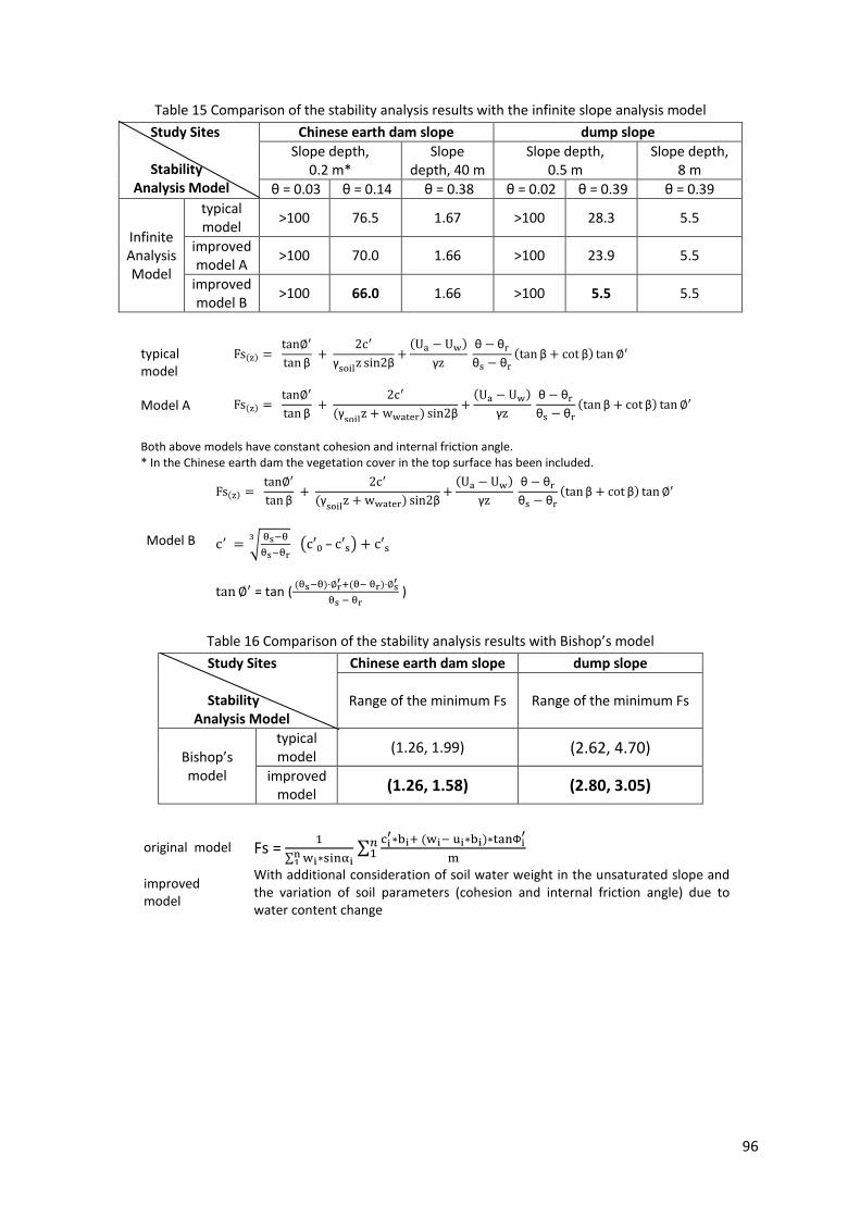
96

Table 15 Comparison of the stability analysis results with the infinite slope analysis model

Study Sites Stability Analysis Model

Chinese earth dam slope dump slope

Slope depth, 0.2 m*

Slope depth, 40 m

Slope depth, 0.5 m

Slope depth, 8 m

θ = 0.03 θ = 0.14 θ = 0.38 θ = 0.02 θ = 0.39 θ = 0.39

Infinite Analysis Model

typical model

>100 76.5 1.67 >100 28.3 5.5

improved model A

>100 70.0 1.66 >100 23.9 5.5

improved model B

>100 66.0 1.66 >100 5.5 5.5

typical model

β

γ β

γ

θ θ

θ θ

β β

Model A

β

γ

β

γ

θ θ

θ θ

β β

Both above models have constant cohesion and internal friction angle. * In the Chinese earth dam the vegetation cover in the top surface has been included.

Table 16 Comparison of the stability analysis results with Bishop’s model

Study Sites Stability Analysis Model

Chinese earth dam slope dump slope

Range of the minimum Fs Range of the minimum Fs

Bishop’s model

typical model

(1.26, 1.99) (2.62, 4.70)

improved model (1.26, 1.58) (2.80, 3.05)

original model Fs =

Ф

improved model

With additional consideration of soil water weight in the unsaturated slope and the variation of soil parameters (cohesion and internal friction angle) due to water content change

Model B

β

γ

β

γ

θ θ

θ θ

β β

–

= tan (

)

97

CHAPTER 8 Conclusions and Recommendation

8.1 Conclusions

Earth dam and dike slope instability is a major concern in both China and Germany where

slope failures have caused catastrophic destruction on the surrounding areas. The slope

stability might be determined by various external or internal factors which result in the

imbalance of forces inside the slope. The external factors include the external loading force,

e.g. the human activities and the large vegetation on the slope; while the internal triggering

factors mainly refer to the internal changes among which the increasing water content in the

unsaturated slope and the decrease of soil properties in the soil play the significant role on

the slope instability.

The hydrological process and water content (water saturation) in the earth slope can be

exactly simulated by the program PCSiWaPro® which has several advantages, e.g. different

options for the pedotransfer functions to calculate the van Genuchten-Luckner parameters,

setup of weather generator and data calibration system. By the weather generator a much

better resolution of the hydrological process simulation can be achieved in the earth slopes

either during the dry season or during the rainfall event; the strong calibration system

between the measured values and simulation results inside PCSiWaPro® has been proved to

be favorably applicable in both the Chinese earth dam slopes and the sandy dump slope.

Conclusions and some experiences with the application of the program PCSiWaPro® are

listed below:

1) The simulation results by the program PCSiWaPro® for the physical dam model in the

laboratory indicated clearly that groundwater flow had been already detected in the

highly saturated dam body.

2) With the program PCSiWaPro®, water content and saturation distribution in the

slope zone could be simulated and predicted dynamically within the whole study

period, which was the preliminary work for stability analysis by the infinite slope

model.

3) These studies also showed the availability of PCSiWaPro® to simulate and predict

groundwater level variations in observation wells within a continuous period.

4) The agreement between the measured groundwater levels and the computed ones

using PCSiWaPro® was good for our real study areas (the Chinese earth dam and the

dump slope of the mining pit). However, there was a little deviation between those

two values, especially in the Chinese earth dam slope. These deviations could be

caused by poorly estimated soil parameters (e.g. porosity, hydraulic conductivity)

which are based on the given DIN 4220 values. In this case, more investigation work

for those soil parameters in both the field and the laboratory is in great need in order

to get better matching between the PCSiWaPro® simulation and real observation.

98

As being discussed in this study, the water content can contribute to the decrease of the

factor of safety (Fs) in the earth slope; in order to investigate how the water content can

reduce the slope stability, two approaches of stability analysis, one based on the Infinite

Slope Model and the other carried out by the Limit Equilibrium Method (like the Bishop’s

model), have been widely applied with the advantage of the Mohr-Coulomb criterion which

expresses the shear strength between the slope soil layers. The infinite slope analysis has an

advantage of easy and quick application for the stability analysis especially for the surficial

landslide forecasting; while the limit equilibrium method is more professional for the deep

circular slip surface analysis.

The stability evaluation of the earth slope in the case studies from China and Germany

utilizes both the common analytical approaches and the improved ones based on the

variation of soil parameters (cohesion and internal friction angle) in the saturated and

unsaturated soils. Several conclusions were achieved as shown below:

1) Vegetation on the air side of dams and dikes has significant influence on the stability

of slopes from the root cohesion as well as water uptake by plant roots.

2) The influence of infiltrated rainfall in the unsaturated slope has been proved to be a

negative contribution to the slope stability especially for the upper subsurface layer.

3) The additional consideration of water content has resulted in a smaller Fs value when

applying the infinite slope model in the unsaturated slope (especially in the

subsurface layer and under the heavy rainfall event).

4) In the deeper layer of the slope under the saturated condition, the infinite slope

model told us that there was no clear difference between the Fs values for the

different depths.

5) By the infinite slope model, the Chinese earth dam has been found to be unstable

and for the deeper layer of the Chinese earth dam, necessary prevention work was in

great need to reduce the possible deep landslide; while the dump slope from the

mining area has been proved to be very stable according to the two stability analysis

models.

6) Practically, with the water content simulation or prediction results (especially in the

heavy rainfall event) from the program PCSiWaPro®, the infinite slope stability

analysis model can be taken as a powerful tool for forecasting the possible surficial

landslides.

7) Combination of the program PCSiWaPro® and the improved Bishop’s model can

provide us an applicable tool for the determination of the size and the structure (e.g.

the core and the slope angle) for a safe earth dam and dike.

As a summary of the above discussed conclusions, the hydrological process in the earth

slope can be simulated by the program PCSiWaPro® which provides the accurate position of

the seepage line and water content distribution in the unsaturated slope; with this

simulation results, two stability analysis models (the Infinite Slope Analysis Model and the

Bishop’s model) have been applied with additional consideration of the influence from

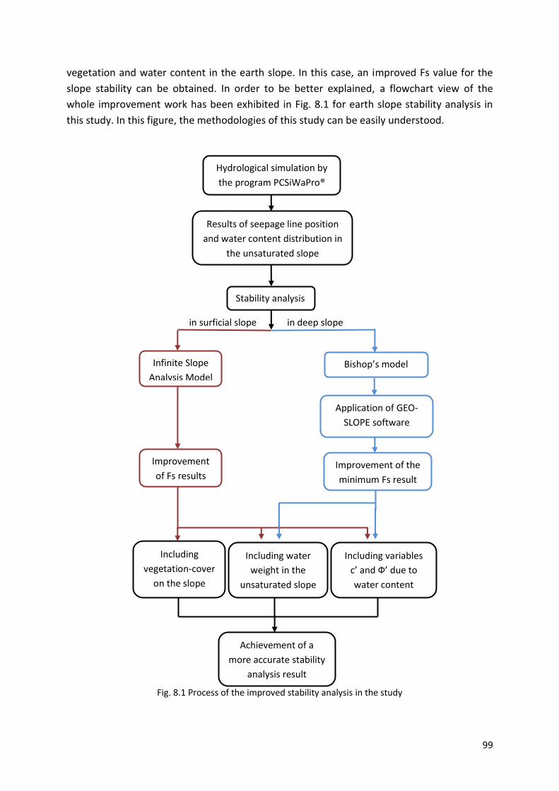
99

vegetation and water content in the earth slope. In this case, an improved Fs value for the

slope stability can be obtained. In order to be better explained, a flowchart view of the

whole improvement work has been exhibited in Fig. 8.1 for earth slope stability analysis in

this study. In this figure, the methodologies of this study can be easily understood.

in surficial slope in deep slope

Fig. 8.1 Process of the improved stability analysis in the study

Achievement of a

more accurate stability

analysis result

Hydrological simulation by

the program PCSiWaPro®

Results of seepage line position

and water content distribution in

the unsaturated slope

Stability analysis

Infinite Slope

Analysis Model

Improvement

of Fs results

Including

vegetation-cover

on the slope

Including water

weight in the

unsaturated slope

Including variables

c’ and Ф’ due to

water content

change

Bishop’s model

Application of GEO-

SLOPE software

Improvement of the

minimum Fs result

100

8.2 Recommendation and further research work

As being discussed in the thesis, the program PCSiWaPro® provides us a powerful and

accurate tool to investigate the hydrological regime in the earth dam and dike slope;

however, the existing soil database DIN4220 in the program (e.g. hydraulic conductivity,

residual water content, porosity, van Genuchten parameters) and the geo-data (e.g.

cohesion, internal friction angle) from the references were applied directly to the simulation

work for our study cases both in China and in Germany instead of the tested data. This could

cause the uncertainty of the analysis results. In this reason, it is highly recommended to

collect real soil data in practice in order to achieve better hydrological simulation results and

more accurate stability analysis.

Furthermore, the models to express the relationship between the water content and soil

property parameters (cohesion and internal friction) are theoretically based on simple

assumptions (e.g. only spherical pore space in soil, pores with the same change rate of

wetting and drying) and empirical results (negative linear relationship between water

content and internal friction angle). In this reason, more field and laboratory work is found

useful in order to improve the parameter values and promote the applicability. In addition,

the effect of vegetation on the slope stability in this study has been calculated by an

empirical equation which has also brought up some inaccuracy; in this reason, in the

laboratory more experiments are needed to test the shear stress from certain vegetation

within certain coverage on the earth slope.

In this study, only the infinite slope analysis and the Bishop’s model have been implemented

and improved with additional consideration of the influence of water content in the

unsaturated slope on the stability which has greatly enhanced the accuracy of the landslide

forecasting. In the future, other stability models, like the ordinary method of slices and the

Spencer method, can be also utilized and improved in the practice with the input of water

content.

101

References:

Abe, K. (1997): A method of evaluating the effect of trees roots on preventing shallow-

seated landslides, Bull. Forest. Forest Prod. Res. Inst. 1 (373), pp.1105–1181.

AgriInfo.in (2011): Classification of soil water, Introduction to Soil Science.

http://www.agriinfo.in/?page=topic&superid=4&topicid=279

Aigner, D. (2004): Auswertung von Untersuchungen über den Einsatz einer

Gummispundwand sowie einer Sickerleitung an einem durchströmten Modelldeich, Institut

für Wasserbau und Technische Hydromechanik Dresden, Technische Universität Dresden.

Arunan, E., Desiraju, G. R., Klein, R. A., Sadlej, J., Scheiner, S., Alkorta, I., Clary, D. C., Crabtree,

R. H., Dannenberg, J. J., Hobza, P., Kjaergaard, H. G., Legon, A. C., Mennucci, B. and Nesbitt,

D. J. (2011): Defining the hydrogen bond: An account (IUPAC Technical Report), Pure Appl.

Chem. 83, pp. 1619-1636.

Aryal, K. P. (2006): Slope Stability Evaluations by Limit Equilibrium and Finite Element

Methods, Norwegian University of Science and Technology.

ASTM International (2011): ASTM D2487-11, Standard Practice for Classification of Soils for

Engineering Purposes (Unified Soil Classification System), West Conshohocken, PA.

www.astm.org

Bassell, B. (1904): Earth dam, a study, The Engineering News Publishing Company.

Beal, P.E. (1987): Estimation of the shear strength of root reinforced soils, Master Thesis,

Ohio State University, Colombus, OH.

Bear, J. (1972): Dynamics of Fluids in Porous Media, Dover, ISBN 0-486-65675-6.

Bian, J. and Wang, B. (2011): Research on Influence of Water Contents on the Shear Strength Behavior of Unsaturated Soils, Chinese Journal of Underground Space and Engineering.

Biondi, G., Cascone, E., Maugeri, M. and Motta, E. (2000): Seismic response of saturated cohesionless slopes, Soil dynamics and earthquake engineering, 20, pp. 209–215.

Bonelli, S. (2013): Erosion in geomechanics applied to dams and levees, Wiley-ISTE, ISBN: 978-1-84821-409-5.

Bowles, J. E. (1988): Foundation Analysis and Design, 4th Edition, McGraw-Hill.

Brueckner, F., Ceranski, H., Mansel H. and Uhlig, C. (2013): Impacts of Re-Rising Groundwater

Levels in Rehabilitated Opencast Mining Areas-Prediction Tools and Potential Measures of

Damage Limitation, IMWA 2013.

102

Caine, N. (1980): The rainfall intensity-duration control of shallow landslides and debris flows, Geografiska Annaler, 62A, pp. 23-27.

Carter, M. and Bentley, S. (1991): Correlations of soil properties, Penetech Press Publishers,

London.

Chanson, H. (2004): Hydraulics of Open Channel Flow: An Introduction, Butterworth–

Heinemann, ISBN 0750659785, pp. 22.

Coppin, N.J., Barker, D.H. and Richards, I. (1990): Use of Vegetation in Civil Engineering, Butterworths, Sevenoaks, Kent.

Coppin, N.J., and Richards, I.G. (1990): Use of vegetation in civil engineering, Butterworths,

London.

Corominas, J. and Moya, J. (1999): Reconstructing recent landslide activity in relation to rainfall in the Llobregat River basin, Eastern Pyrenees, Spain, Geomorphology, 30, pp.79-93.

Coulomb, C. A. (1776): Essai sur une application des règles des maximis et minimis à

quelques problèmes de statique relatifs, à la architecture. Mem. Acad. Roy. Div. Sav., vol. 7,

pp. 343–387.

Darcy, H. (1856): Les Fontaines Publiques de la Ville de Dijon, Dalmont, Paris.

De Baets, S., Poesen, J., Reubens, B., Wemans, K., De Baerdemaeker, J., and Muys, B. (2008):

Root tensile strength and root distribution of typical Mediterranean plant species and their

contribution to soil shear strength, Plant Soil (2008) 305, pp. 207–226.

Deng, W. D., Deng, C. Z. and Yan, Q. R. (2008): Study on direct shear test on interface

performance of geogrid and coarse grained soil, Proceedings of the 4th Asian Regional

Conference on Geosynthetics, June 17-20, 2008, Shanghai, China.

Dinesh, S. V. (2014): Stability of Earth Slopes, Civil Engineering Department, Siddaganga

Institute of Technology.

Duncan, J. M. and Wright, S. G. (2005): Soil strength and slope stability, John Wiley, Hoboken

N. J.

Endo, T. and Tsuruta, T. (1969): The effect of tree roots on the shearing strength of soil,

Annual Report, Forest Experiment Station, Hokkaido, pp. 451-461.

Ersayin, D. (2006): Studying seepage in a body of the earth-filled dam by (artificial neural networks) ANNs, Master Thesis, Department of Civil Engineering, İzmir Institute of Technology, 150 p.

103

Faculty of Geography, University of Victoria: Mountain Slope Stability and Land Use,

presentation. www.geog.uvic.ca/geog476/mtstability.pdf

Fattah Mohammed Y., Yahya, A. Y., Maysam Th. A. and Ahmed, B. A. (2013): Effect of salt

content on total and matric suction of unsaturated soils, European Scientific Journal.

Food and Agriculture Organisation of the United Nations (2007): Introduction to evapo-

transpiration. http://www.fao.org/docrep/X0490E/x0490e04.htm

Fredlund, D. G. and Rahardjo, H. (1993): Soil mechanics for unsaturated soils, published by

John Wiley & Sons, Inc. ISBN: 9780471850083.

Fredlund, D.G., Rahardjo, H. and Ng, T. (1993): Effect of pore air and negative pore water

pressures on stability at the end-of-construction, Proceedings of International Conference on

Dam Engineering, Johor Bahru, Malaysia, January 12-13, 1993.

Fredlund, D.G., Morgenstern, N.R. and Widger, R.A. (1978): Shear strength of unsaturated

soils, Can.Geotech.J. 15, pp. 313-321.

Geotechdata.info (2013): Angle of Friction. http://geotechdata.info/parameter/angle-of-

friction.html

Geotechdata.info (2013): Cohesion. http://geotechdata.info/parameter/cohesion

Giglou, A. N. and Zeraatparvar, A. (2012): Seepage Estimation through Earth Dams, Journal of Basic and Applied Scientific Research, 2(8), 2012, pp. 7861-7865.

Golder Associates Ltd. and Associated Engineering (B.C.) Ltd. (2003): Dike Design and Construction Guide Best Management Practices For British Columbia, Flood Hazard Management Section Environmental Protection Division Province of British Columbia Ministry of Water, Land and Air Protection.

Gonzalez, P. A. and Adams, B. J. (1980): Mine Tailings Disposal: I. Laboratory Characterization of Tailings, Dep. of Civil Eng., Univ. of Toronto, Toronto, Ont., Canada, pp. 1-14.

Gover, S. and Hammah, R. (2013): A comparison of finite elements (SSR) and limit-equilibrium slope stability analysis by case study, Golder Associates Africa (Pty) Ltd.

Graeber, P-W, Blankenburg, R., Kemmesies, O. and Krug, S. (2006): SiWaPro DSS -

Beratungssystem zur Simulation von Prozessen der unterirdischen Zonen. [Buchverf.] Jochen

Wittmann und Mike Müller. [Hrsg.] Mike Müller. Simulation in Umwelt- und

Geowissenschaften. Leipzig: Shaker Verlag, 2006, pp. 25-234.

Gray, D.H. (1995): Influence of vegetation on the stability of slopes, In: Barker, D.H. (Ed.), Vegetation and Slopes Stabilisation, Protection and Ecology, Thomas Telford House, London, pp. 2–23.

104

Gray, D. H. and Leiser, A. T. (1982): Biotechnical slope protection and erosion control, Van

Nostrand Reinhold Company, New York.

Gray, D.H. and Megahan, W.F. (1981): Forest vegetation removal and slope stability in the

Idaho Batholith, Internmountain Forest and Range Experiment Station, U.S. Forest Service,

Ogden, Utah, Research Paper INT-271.

Gray, D.H., and Sotir, R.B. (1996): Biotechnical and soil bioengineering slope stabilization,

John Wiley and Sons, New York.

Greenway, D. T. (1987): Vegetation and slope stability, in Slope Stability (eds M.G. Anderson

and Richards K.S.), John Wiley, New York, pp.187-230.

Greenwood, J., Norris, J. and Wint, J. (2004): Assessing the contribution of vegetation to

slope stability, Proceedings of the Institution of Civil Engineers, vol. 157, no. 4, pp. 199-207.

Griffiths, D.V., Huang, J. and Fenton, G. A. (2011): Probabilistic infinite slope analysis,

Computers and Geotechnics 38 (2011), pp. 577–584.

Hammond, C.; Hall, D. E.; Miller, S., and Swetik, P. (1992): Level I Stability Analysis (LISA)

Documentation for Version 2.0: U.S. Department of Agriculture, Forest Service,

Intermountain Research Station; General Technical Report INT-285, Ogden, UT, 190 p.

Han, J., Chai, J., Leshchinsky, D., and Shen, S., (2004): Evaluation of Deep-Seated Slope

Stability of Embankments over Deep Mixed Foundations, Geotechnical Special Publication

No. 124, J.P. Turner and P.W. Mayne (eds), GeoSupport 2004, ASCE Geo-Institute and ADSC,

Jan. 29-31, Orlando, pp. 945-954.

Hasan, I., Meyer, M. and Graeber, P.-W. (2012): Simulation des Wasserhaushalts in

Erddämmen und Deichen als Basis für Stabilitätsuntersuchungen mit dem Programm

PCSiWaPro®, Institut für Abfallwirtschaft und Altlasten, Technische Universität Dresden.

Hathaway, R.L. (1973): Factor affecting the soil binding capacity of the root system of some

Populus and Salix clones, Mater Thesis, Massey Univerity, Palmerston North.

Hathaway, R.L. and Penny, D. (1975): Root strength in some populous and salix clones, New

Zealand J. Botany, 13, pp. 333-344.

Heath, R.C. (1983): Basic ground-water hydrology, U.S. Geological Survey Water-Supply

Paper 2220, 86 p.

Hoffman, G., Hoven, A. V. and Verheij, H. (2010): Instability of grass caused by wave

overtopping, Scour and erosion, Proceedings of the fifth International Conference on Scour

and Erosion (ICSE-5), November 7 - 10, 2010, San Francisco, California, USA.

105

Hossain, Md. K. (2010): Effect of Rainfall on Matric Suction and Stability of a Residual Granite

Soil Slope, DUET Journal.

Huang, B. and Nobel, P.S. (1994): Root hydraulic conductivity and its components with emphasis on desert succulents, Agron. J. 86, pp. 767–774.

ikos-team (2007): Causes of landslides.

http://en.wikipedia.org/wiki/User:Multichill/top_self_uploaders/Oikos-team

Israelachvili J. (1990): Intermolecular and Surface Forces, Academic Press, San Diego, editor.

Israelachvelli J.N. (1991): Intermolecular and Surface Forces, Academic Press, London.

IUPAC (1997): Compendium of Chemical Terminology, 2nd ed. (the "Gold Book"), Online

corrected version: (1994) "van der Waals forces".

Jonkman, B., Schweckendiek T., Dupuits G., Heyer T., de Bijl J. and Labrujere A. (2013): Floods in Germany (2013) – post-flood field investigation, TU Delft, Technische Unversitaet Dresden in collaboration with stowa.

Juvinal, R. C. and Marshek, K. M. (1991): Fundamentals of machine component design – 2nd

ed., ISBN 0-471-62281-8, pp. 217.

Keefer, D.K. (1984): Landslides caused by earthquakes, Bulletin of the Geological Society of

America 95, pp. 406-421.

Kemmesies, O. (1995): Prozessmodellierung und Parameteridentifikation von Mehrphasenströmungsprozessen in porösen Medien. Dresden: Dresdner Grundwasserforschungszentrum e.V., 1995, ISSN 1430-0176.

Kemper, W. D. and Rosenau, R. C. (1984): Soil Cohesion as Affected by Time and Water Content, Soil Science Society of America Journal.

Kim, Y. T., Shin, H. and Park, D. K. (2011): Variation of shear strength of weathered granite

soil with water content, Unsaturated Soils: Theory and Practice 2011, Jotisankasa,

Sawangsuriya, Soralump and Mairaing (Editors), Kasetsart University, Thailand, ISBN 978-

616-7522-77-7.

Koloski, J. W., Schwarz, S. D. and Tubbs, D. W. (1989): Geotechnical Properties of Geologic

Materials, Engineering Geology in Washington, Volume 1, Washington Division of Geology

and Earth Resources Bulletin 78.

Krahn, J. (2004): Stability Modelling with Slope/W, an engineering methodology, Geo-

slope/W International, Ltd.

106

Leiser, A. T. (1998): Bio-technology for slope protection and erosion control, University of

California, Davis, California.

Li, H. M. (2005): Impact of cohesion forces on particle mixing and segregation, University of Pittsburgh.

Lu, N., and Godt J. W. (2008): Infinite-slope stability under steady unsaturated conditions, Water Resour. Res., 44, W11404, doi: 10.1029/ 2008WR00697.

Lu, N., and Likos W. J. (2006): Suction stress characteristic curve for unsaturated soil, J. Geotech. Geoenviron. Eng., 123, pp. 131–142.

Lv, X., Cui, K., Li, D. and Zhou, Y. (2010): Soil slope stability factors analysis based on PLAXIS, Journal of Anhui Institute of Architecture & Industry, 2010.

Malgot, J. and Baliak, F. (2002): Influence of human activity on the development of landslides

in Slovakia, Geografický časopis, 54.

Menashe, E. (1998): Vegetation and Erosion—A Literature Survey, in Proceedings of the

Native Plants Symposium, Oregon State University, Forest Science Lab., Corvallis, OR., Dec. 9-

10, 1998, pp.130-135.

Meyerhof, G. (1956): Penetration tests and bearing capacity of cohesionless soils, Journal of

Soils Mechanics and Foundation, Division ASCE, 82 (SM1).

Minnesota Department of Transportation (2007): Pavement Design.

http://www.dot.state.mn.us/materials/pvmtdesign/manual.html

Moayed, R. Z., Rashidian, V., and Izadi, E. (2012): Evaluation of phreatic line in the

homogenous earth dams with different drainage systems, Proceeding of Innovative Dam and

Levee Design and Construction for Sustainable Water Management, 32nd Annual USSD

Conference New Orleans, Louisiana, April 23-27, 2012.

Morgan, R. P. C. and Rickson, R. J. (1996): Slope stabilization and eriosion control, a

bioengineering approach; E and FN SPON.

Mulley, R. (2004): Flow of Industrial Fluids: Theory and Equations, CRC Press,

ISBN 0849327679, 410 pages, pp. 43–44.

Nase, S. T. (2000): Characterization of wet granular flow: application to mixing and segregation, Master Thesis, University of Pittsburgh.

NAVFAC Design Manual 7.2: Foundations and Earth Structures, SN 0525-LP-300-7071,

revalidated by change 1 September 1986.

107

Nelson, S. A. (2011): Physical Geology, Tulane University. http://www.tulane.edu/~sanelson/geol111/groundwater.htm

Nilaweera, N.S. (1994): Effect of tree roots on slope stability: the case of Khao Luang

Mountain area, southern Thailand, Doc. of Tech. Sci. thesis, Asian Institute of Technology,

Bangkok, Thailand.

NPTEL: Lecture notes for Hydraulic Structures for Flow Diversion and Storage, Department of

Civil Engineering, National Program on Technology Enhanced Learning.

http://nptel.ac.in/courses/105105110/pdf/m4l07.pdf

NYSDEC (New York State Department of Environmental Conservation) (1987): Owners

Guidance Manual for the Inspection and Maintenance of Dams in NYS.

O'Loughlin, C. (1974): The effect of timber removal on the stability of forest slopes, Journal

of Hydrology, New Zealand, 13, pp. 121–134.

Obrzud R. and Truty, A. (2012): The hardening soil model - A practical guidebook Z Soil, PC

100701 report, revised 31.01.2012.

Osman, N. and Barakabah, S. (2006): Parameters to predict slope stability – Soil water and root profiles, Ecological Engineering, vol. 28, no. 1, pp. 90-95.

Peck, R., Hanson,W., and Thornburn, T. (1974). Foundation Engineering Handbook, Wiley, London.

Perry, J., Pedley, M. and Reid, M. (2003): Infrastructure embankments condition appraisal and remedial treatment, MWL Digital, Pontypool, South Wales.

Pervizpour, M. (2004): Performance evaluation of constructed facilities, Wiedner University.

Rhodes M. (1998): Introduction to particle technology, John Wiley and Sons, New York.

Riestenberg, M.M., and Sovonick-Dunford, S. (1983): The role of woody vegetation in stabilizing slopes in the Cincinnati area. Geological Society of America Bulletin, 94: 506–518.

Schiechtl, H.M. (1980): Bioengineering for land reclamation and conservation, University of Alberta Press, Edmonton.

Schuettrumpf, H. (2008): Aktuelle Entwicklungen im internationalen Küsteningenieurwesen - International Conference on Coastal Engineering, In: Korrespondenz Wasserwirtschaft: KW. - Hennef: GFA. - ISSN: 1616-430X, 1865-9926. - 1 (2008) 12, S./Art., pp. 664-665.

Sellmeijer, J.B., Lopez D. L. C. J., Beek V. M. V. and Knoeff J.G. (2011): fine tuning of the

piping model through small-scale, medium-scale and IJkdijk experiments, European Journal

of Environmental and Civil Engineering, vol.15, no.8, pp.1139-1154.

108

Shi, W., Liao, Y. and Tang, X. (2011): Study of the relationship between water content and

shear strength of Guiyang red clay, Subgrade Engineering.

Skempton, A.W. and DeLory, F.A. (1957): Stability of Natural Slopes in London Clay, Proceedings 4th International Conference on Soil Mechanics and Foundation Engineering, Rotterdam.

Staatsministerium fuer Umwelt und Landwirtschaft (2007): Hochwasserschutz in Sachsen.

Styczen, M. E. and Morgan, R. P. C. (1995): Engineering properties of vegetation, In: Slope Stabilization and Erosion control: A Bioengineering approach, Morgan R.P.C. and R.J. Rickson, (Eds.), E and F.N. Spon, London, pp. 5-58.

Swanston, D. N. (1970): Mechanics of debris avalanching in shallow till soils of southeastern Alaska, Forest Service, Research Paper PNW 103, US Dept. of Agriculture.

Swiss Standard SN 670 010b: Characteristic Coefficients of soils, Association of Swiss Road and Traffic Engineers.

System Analysis Group: Presentation of the project ‘Effiziente Grundwassersimulation bei der Gewinnung von Energieressourcen’, Faculty of Environmental Sciences, Technische Universität Dresden.

Tang, D., Peng, J. and Sun, W. (2012): Matrix suction test based on the filter paper method for unsaturated loess, COAL GEOLOGY & EXPLORATION.

Taylor, D. W. (1937): Stability of earth slopes, J. Boston Soc. Civil Eng., 24(3), Reprinted in:

Contributions to Soil Mechanics 1925 to 1940, Boston Society of Civil Engineers, pp. 337–386.

Teepe, R.; Dilling, H. and Beese, F. (2003): Estimating water retention curves of forest soils from soil texture and bulk density, J. Plant Nutr. Soil Sci. 166, pp. 111-119.

Terwilliger, V.J. (1988): Mechanical effects of chaparral disturbance on soil slip patterns in the transverse ranges of Southern California, PhD Dessitation, University of California, Los Angeles, CA.

Thielen, A. (2007). Einfluss der Bodensaetigung auf die Stabilitaet von Haengen (Influence of soil saturation on the stability of slopes), ETH-Diss.Nr. 17303: http://ecollection.ethbib.ethz.ch/view/eth:29862.

Tsukamoto, Y., and Kusaba, O. (1984): Vegetative influence on debris slide occurrences on steep slopes in Japan, In Proceedings of the Symposium on Forest Land Use on Erosion and Slope Stability, Environmental Policy Institute, Honolulu, Hawaii.

U.S.A.C.E. (2004): Engineering and Design, General Design and Construction Considerations for Earth and Rock-fill Dams, US Army Corps of Engineers®.

109

United States. Bureau of Reclamation (1987): Embankment dams, Denver, Colo.: U.S. Dept.

of the Interior, Bureau of Reclamation, Engineering and Research Center.

U.S. Environmental Protection Agency (2009): Glossary of technical terms, U.S.

Environmental Protection Agency, access date July 22, 2010.

USGS (2004): Landslide Types and Processes.

http://pubs.usgs.gov/fs/2004/3072/pdf/fs2004-3072.pdf

USGS (1988): Definitions of selected ground-water terms--Revisions and conceptual

refinements, Committee on Redefinition of Ground-Water Terms, U.S. Geological Survey

Water-Supply Paper 1988, pp. 26.

Vereecken, H., Feyen, J., Maes, J. and Darius, P. (1989): Estimating the soil moisture

retention characteristic from texture, bulk density, and carbon content, Soil Sci. 148, pp.

389-403.

Watts, P. J., Cox, G. J. and Stepnuk, L. M. (2001): Farm Dams for the Sugar Industry, FSA Consulting.

Waldron, L.J. (1977): The shear resistance of rootpermeated homogeneous and stratified soil, Journal of Soil Science, Soc. Am., 41, pp. 843-849.

Waldron, L.J. and Dakessian, S. (1981): Soil reinforcement by roots, calculation of increased shear resistance from root properties, Soil Science, 132, pp. 427-435.

Weynants, M., Vereecken, H. and Javaux, M. (2009): Revisiting Vereecken pedotransfer functions: Introducing a closed-form hydraulic model, Vadose Zone J. 8, pp. 86–95.

Wu, T.H. (1984a): Effect of vegetation on slope stability, in Soil Reinforcement and Moisture Effect on Stability, Transportation Research Record 965, Washington, DC, pp. 37–46.

Wu,T.H. (1984b): Soil movement on permafrost slopes near Fairbanks, Alaska, Journal of Canadian Geotechnical, 21, pp. 699-709.

Wu, T.H. (2013): Root reinforcement of soil: Review of analytical models, test results, and applications to design, NRC Research Press.

Wu, T.H., Beal, P.E. and Lan, C (1988a): In situ shear tests of soil root system, Journal of Geotechnical Engineering, ASCE, 114, pp1376-1394.

Wu, T.H., Bettandapura, D.P. and Beal, P.E. (1988b): A statistical model of root geometry, Forest Science, 34, pp. 980-997.

Wu, T.H., McKinnell, W.P. and Swanston, D.N. (1979): Strength of tree roots and landslides on Prince of Wales Island, Alaska, Canadian Geotechnical Journal, 16, pp 19-33.

110

Wu, T.H., McOmber, R.M., Erb, R.T. and Beal, B.E. (1988c): A study of soil root interaction, Journal of Geotechnical Engineering, ASCE, pp 1351-1375.

Wösten, J. H. M., Pachepsky, Y. A. and Rawls, W. J. (2001): Pedotransfer functions: Bridging

the gap between avai lable basic soil data and missing soil hydraulic characteristics, Journal

of Hydrology, 251, pp. 123–150.

Yeh, H., Lee, C. and Lee, C. (2008): A rainfall infiltration model for unsaturated soil slope

stability, J. Environ. Eng. Manage., 18(4), pp. 261-268.

Záruba, Q. and Mencl, V. (1987): Landslides and their control, Amsterdam (Elsevier).

Zhou, W. Y. (1990): Advanced Rock Mechanics (in Chinese), Beijing: China Water Power Press,

pp.46-86.

Ziemer, R. R. (1981): Roots and the stability of forested slopes, in Erosion and Sediment

Transport in Pacific Rim Steeplands, Publication 132, International Association of

Hydrological Sciences, London, pp.343-361.

111

Appendix

Table 1: Cohesion values for different soil types (Geotechdata.info, 2013)

Description USCS Cohesion [kPa] Reference

min max Specific value

Well graded gravel, sandy gravel, with little or no fines

GW - - 0 Swiss Standard SN 670 010b, Minnesota Department of Transportation, 2007, NAVFAC Design Manual 7.2, 1986

Poorly graded gravel, sandy gravel, with little or no fines

GP - - 0 Swiss Standard SN 670 010b, Minnesota Department of Transportation, 2007, NAVFAC Design Manual 7.2, 1986

Silty gravels, silty sandy gravels GM - - 0 Swiss Standard SN 670 010b,

Clayey gravels, clayey sandy gravels

GC - - 20 Swiss Standard SN 670 010b,

Well graded sands, gravelly sands, with little or no fines

SW - - 0 Swiss Standard SN 670 010b, Minnesota Department of Transportation, 2007, NAVFAC Design Manual 7.2, 1986

Poorly graded sands, gravelly sands, with little or no fines

SP - - 0 Swiss Standard SN 670 010b, Minnesota Department of Transportation, 2007, NAVFAC Design Manual 7.2, 1986

Silty sands SM - - 22 Swiss Standard SN 670 010b,

Silty sands - Saturated compacted

SM - - 50 NAVFAC Design Manual 7.2, 1986

Silty sands - Compacted SM - - 20 NAVFAC Design Manual 7.2, 1986

Clayey sands SC - - 5 Swiss Standard SN 670 010b,

Clayey sands - Compacted SC - - 74 NAVFAC Design Manual 7.2, 1986

Clayey sands -Saturated compacted

SC - - 11 NAVFAC Design Manual 7.2, 1986

Loamy sand, sandy clay Loam - compacted

SM, SC 50 75 Minnesota Department of Transportation, 2007,

Loamy sand, sandy clay Loam - saturated

SM, SC 10 20 Minnesota Department of Transportation, 2007,

Sand silt clay with slightly plastic fines - compacted

SM, SC - - 50 NAVFAC Design Manual 7.2, 1986

Sand silt clay with slightly plastic fines - saturated compacted

SM, SC - - 14 NAVFAC Design Manual 7.2, 1986

Inorganic silts, silty or clayey fine sands, with slight plasticity

ML - - 7 Swiss Standard SN 670 010b,

Inorganic silts and clayey silts - compacted

ML - - 67 NAVFAC Design Manual 7.2, 1986

Inorganic silts and clayey silts - saturated compacted

ML - - 9 NAVFAC Design Manual 7.2, 1986

Inorganic clays, silty clays, sandy clays of low plasticity

CL - - 4 Swiss Standard SN 670 010b,

Inorganic clays, silty clays, sandy clays of low plasticity - compacted

CL - - 86 NAVFAC Design Manual 7.2, 1986

Inorganic clays, silty clays, sandy clays of low plasticity - saturated compacted

CL - - 13 NAVFAC Design Manual 7.2, 1986

Mixture if inorganic silt and clay - compacted

ML-CL - - 65 NAVFAC Design Manual 7.2, 1986

Mixture of inorganic silt and clay - saturated compacted

ML-CL - - 22 NAVFAC Design Manual 7.2, 1986

112

Organic silts and organic silty clays of low plasticity

OL - - 5 Swiss Standard SN 670 010b,

Inorganic silts of high plasticity - compactd

MH - - 10 Swiss Standard SN 670 010b,

Inorganic silts of high plasticity - saturated compacted

MH - - 72 NAVFAC Design Manual 7.2, 1986

Inorganic silts of high plasticity MH - - 20 NAVFAC Design Manual 7.2, 1986

Inorganic clays of high plasticity

CH - - 25 Swiss Standard SN 670 010b,

Inorganic clays of high plasticity - compacted

CH - - 103 NAVFAC Design Manual 7.2, 1986

Inorganic clays of high plasticity - saturated compacted

CH - - 11 NAVFAC Design Manual 7.2, 1986

Organic clays of high plasticity OH - - 10 Swiss Standard SN 670 010b,

Loam - Compacted ML, OL, MH, OH 60 90 Minnesota Department of Transportation, 2007,

Loam - Saturated ML, OL, MH, OH 10 20 Minnesota Department of Transportation, 2007,

Silt Loam - Compacted ML, OL, MH, OH 60 90 Minnesota Department of Transportation, 2007,

Silt Loam - Saturated ML, OL, MH, OH 10 20 Minnesota Department of Transportation, 2007,

Clay Loam, Silty Clay Loam - Compaced

ML, OL, CL, MH, OH, CH

60 105 Minnesota Department of Transportation, 2007,

Clay Loam, Silty Clay Loam - Saturated

ML, OL, CL, MH, OH, CH

10 20 Minnesota Department of Transportation, 2007,

Silty clay, clay - compacted OL, CL, OH, CH 90 105 Minnesota Department of Transportation, 2007,

Silty clay, clay - saturated OL, CL, OH, CH 10 20 Minnesota Department of Transportation, 2007,

Peat and other highly organic soils

Pt - -

Table 2 Unified Soil Classification System (ASTM International, 2011)

113

Table 3 Engineering properties of earth dam materials (Watts et al., 2001)

Notes: (a) * denotes insufficient data available: (b) values given are averages and ± shows the 90% confidence limits of the averages of groups of samples

Table 4 Typical data of soil internal friction angle for different soils according to USCS (Geotechdata.info,

2013)

Description USCS Soil friction angle [°]

Reference min max

Specific value

Well graded gravel, sandy gravel, with little or no fines

GW 33 40 Swiss Standard SN 670 010b, Koloski et al., (1989)

Poorly graded gravel, sandy gravel, with little or no fines

GP 32 44 Swiss Standard SN 670 010b

Sandy gravels - Loose (GW, GP) 35

Carter and Bentley, (1991), Meyerhof (1956), Peck et al., (1974), Obrzud and Truty (2012)

Sandy gravels - Dense (GW, GP) 50

Carter and Bentley, (1991), Meyerhof (1956), Peck et al., (1974), Obrzud and Truty (2012)

Silty gravels, silty sandy gravels GM 30 40 Swiss Standard SN 670 010b

Clayey gravels, clayey sandy gravels

GC 28 35 Swiss Standard SN 670 010b

Well graded sands, gravelly sands, with little or no fines

SW 33 43 Swiss Standard SN 670 010b

Well-graded clean sand, gravelly sands - Compacted

SW - - 38

Carter and Bentley, (1991), Meyerhof (1956), Peck et al., (1974), Obrzud and Truty (2012)

Well-graded sand, angular grains - Loose

(SW) 33

Carter and Bentley, (1991), Meyerhof (1956), Peck et al., (1974), Obrzud and Truty (2012)

Well-graded sand, angular grains - Dense

(SW) 45

Carter and Bentley, (1991), Meyerhof (1956), Peck et al., (1974), Obrzud and Truty (2012)

Poorly graded sands, gravelly sands, with little or no fines

SP 30 39 Swiss Standard SN 670 010b, Koloski et al., 1989

Poorly-garded clean sand - Compacted

SP - - 37

Carter and Bentley, (1991), Meyerhof (1956), Peck et al., (1974), Obrzud and Truty (2012)

Uniform sand, round grains - (SP) 27 Carter and Bentley, (1991), Meyerhof (1956),

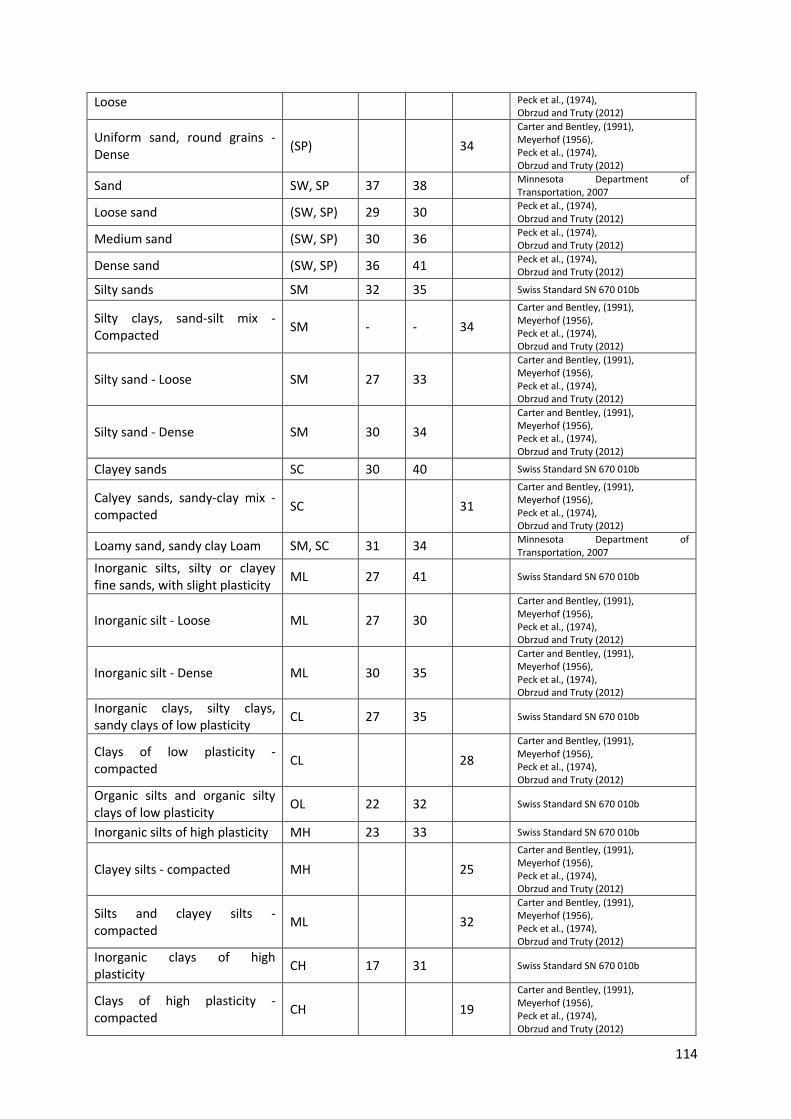
114

Loose Peck et al., (1974), Obrzud and Truty (2012)

Uniform sand, round grains - Dense

(SP) 34

Carter and Bentley, (1991), Meyerhof (1956), Peck et al., (1974), Obrzud and Truty (2012)

Sand SW, SP 37 38 Minnesota Department of Transportation, 2007

Loose sand (SW, SP) 29 30 Peck et al., (1974), Obrzud and Truty (2012)

Medium sand (SW, SP) 30 36 Peck et al., (1974), Obrzud and Truty (2012)

Dense sand (SW, SP) 36 41 Peck et al., (1974), Obrzud and Truty (2012)

Silty sands SM 32 35 Swiss Standard SN 670 010b

Silty clays, sand-silt mix - Compacted

SM - - 34

Carter and Bentley, (1991), Meyerhof (1956), Peck et al., (1974), Obrzud and Truty (2012)

Silty sand - Loose SM 27 33

Carter and Bentley, (1991), Meyerhof (1956), Peck et al., (1974), Obrzud and Truty (2012)

Silty sand - Dense SM 30 34

Carter and Bentley, (1991), Meyerhof (1956), Peck et al., (1974), Obrzud and Truty (2012)

Clayey sands SC 30 40 Swiss Standard SN 670 010b

Calyey sands, sandy-clay mix - compacted

SC 31

Carter and Bentley, (1991), Meyerhof (1956), Peck et al., (1974), Obrzud and Truty (2012)

Loamy sand, sandy clay Loam SM, SC 31 34 Minnesota Department of Transportation, 2007

Inorganic silts, silty or clayey fine sands, with slight plasticity

ML 27 41 Swiss Standard SN 670 010b

Inorganic silt - Loose ML 27 30

Carter and Bentley, (1991), Meyerhof (1956), Peck et al., (1974), Obrzud and Truty (2012)

Inorganic silt - Dense ML 30 35

Carter and Bentley, (1991), Meyerhof (1956), Peck et al., (1974), Obrzud and Truty (2012)

Inorganic clays, silty clays, sandy clays of low plasticity

CL 27 35 Swiss Standard SN 670 010b

Clays of low plasticity - compacted

CL 28

Carter and Bentley, (1991), Meyerhof (1956), Peck et al., (1974), Obrzud and Truty (2012)

Organic silts and organic silty clays of low plasticity

OL 22 32 Swiss Standard SN 670 010b

Inorganic silts of high plasticity MH 23 33 Swiss Standard SN 670 010b

Clayey silts - compacted MH 25

Carter and Bentley, (1991), Meyerhof (1956), Peck et al., (1974), Obrzud and Truty (2012)

Silts and clayey silts - compacted

ML 32

Carter and Bentley, (1991), Meyerhof (1956), Peck et al., (1974), Obrzud and Truty (2012)

Inorganic clays of high plasticity

CH 17 31 Swiss Standard SN 670 010b

Clays of high plasticity - compacted

CH 19

Carter and Bentley, (1991), Meyerhof (1956), Peck et al., (1974), Obrzud and Truty (2012)

115

Organic clays of high plasticity OH 17 35 Swiss Standard SN 670 010b

Loam ML, OL, MH, OH

28 32 Minnesota Department of Transportation, 2007

Silt Loam ML, OL, MH, OH

25 32 Minnesota Department of Transportation, 2007

Clay Loam, Silty Clay Loam ML, OL, CL, MH, OH, CH

18 32 Minnesota Department of Transportation, 2007

Silty clay OL, CL, OH, CH

18 32 Minnesota Department of Transportation, 2007

Clay CL, CH, OH, OL

18 28 Minnesota Department of Transportation, 2007

Peat and other highly organic soils

Pt 0 10 Koloski et al., 1989

Table 5 Root properties of Dutch dike grassland, = / , (Hoffmans et al., 2010)

Table 6 Tensile strength of roots (Morgan and Rickson, 1996)

116

Table 7 Characteristics of excavated root (Morgan and Rickson, 1996)

Table 8 Mean root area ratio (RAR, −) values and standard errors (SE) at different soil depths for typical

Mediterranean plant species (De Baets et al., 2008)

117

Table 9 Calculation of the improved Bishop’s model for the Chinese dam slope (the position of each slice

can be found in Fig. 7.18)

Slice No.

Slice width ( ) m

Weight of dry slice

( ) kN/m

Weight of water in slice kN/m

negative water

pressure force (kN/m)

Base angle

α

sinα *sinα kN/m

Cohesion kPa

*

KN/m

1 3.29 138.6 32.4 0.0 64.9 0.91 154.8 39.4 129.5

2 5.00 667.2 78.9 0.0 61.1 0.87 652.7 48.6 243.0

3 5.00 1113.5 98.6 0.0 56.9 0.84 1015.4 48.6 243.0

4 8.00 2520.6 157.8 0.0 52.2 0.79 2116.1 48.6 388.8

5 8.77 3563.8 173.0 0.0 46.7 0.73 2720.3 48.6 426.3

6 6.08 2841.8 119.9 156.3 42.3 0.67 1886.9 13.1 79.6

7 6.08 3081.3 119.9 439.5 38.9 0.63 1733.4 13.1 79.6

8 6.08 3271.0 119.9 688.2 35.7 0.58 1574.9 13.1 79.6

9 5.25 2944.6 103.6 768.2 32.8 0.54 1233.0 13.1 68.8

10 5.25 3027.9 103.6 907.7 30.1 0.50 1116.3 13.1 68.8

11 5.25 3087.8 103.6 1031.0 27.6 0.46 1000.6 13.1 68.8

12 5.25 3126.0 103.6 1139.2 25.1 0.42 887.1 13.1 68.8

13 5.50 3293.6 108.5 1288.0 22.6 0.38 813.2 13.1 72.1

14 5.50 3290.9 108.5 1363.7 20.1 0.34 700.3 13.1 72.1

15 5.50 3267.1 108.5 1424.8 17.7 0.30 592.4 13.1 72.1

16 5.50 3223.3 108.5 1472.0 15.2 0.26 488.6 13.1 72.1

17 6.00 3443.7 118.4 1645.8 12.7 0.22 422.0 13.1 78.6

18 6.00 3344.0 118.4 1673.0 10.1 0.18 314.7 13.1 78.6

19 6.00 3220.7 118.4 1683.9 7.6 0.13 217.7 13.1 78.6

20 6.00 3074.2 118.4 1678.6 5.0 0.09 132.0 13.1 78.6

21 6.57 3171.5 21.6 1810.2 2.3 0.04 56.2 13.1 86.1

22 6.57 2938.6 0.0 1757.6 0.4 0.01 9.2 13.1 86.1

23 6.57 2676.1 0.0 1684.5 3.2 0.06 55.9 13.1 86.1

24 6.57 2383.7 0.0 1590.6 6.5 0.11 90.0 13.1 86.1

25 5.62 1783.7 0.0 1235.3 8.6 0.15 82.2 13.1 73.6

26 5.62 1528.5 0.0 1058.6 11.0 0.19 90.0 13.1 73.6

27 5.62 1253.7 0.0 868.2 13.5 0.23 89.8 13.1 73.6

28 5.62 958.6 0.0 663.9 15.9 0.27 80.9 13.1 73.6

29 5.62 642.7 0.0 445.1 18.4 0.32 62.4 13.1 73.6

30 5.62 305.0 0.0 211.2 21.0 0.36 33.5 13.1 73.6

31 3.76 43.7 0.0 30.2 23.1 0.39 5.3 13.1 49.3

Silt sand: c’s =13.1 kPa; c’0 = 51.1 kPa; γsoil = 1.415 g/cm3; = 0.01; θ = 0.38

118

Table 10 Calculation of the improved Bishop’s model for the Chinese dam slope (the position of each slice

can be found in Fig. 7.18)

Slice No.

φ' tan φ' Water content

θ

Saturation * + * tanφ'

1 32.7 0.64 0.29 0.76 239.2

2 34.3 0.68 0.09 0.22 751.9

3 34.3 0.68 0.09 0.22 1069.8

4 34.3 0.68 0.09 0.22 2215.8

5 34.3 0.68 0.09 0.22 2975.2

6 32.0 0.62 0.38 1.00 1832.5

7 32.0 0.62 0.38 1.00 1805.2

8 32.0 0.62 0.38 1.00 1768.4

9 32.0 0.62 0.38 1.00 1493.4

10 32.0 0.62 0.38 1.00 1458.3

11 32.0 0.62 0.38 1.00 1418.6

12 32.0 0.62 0.38 1.00 1374.9

13 32.0 0.62 0.38 1.00 1393.0

14 32.0 0.62 0.38 1.00 1344.1

15 32.0 0.62 0.38 1.00 1291.0

16 32.0 0.62 0.38 1.00 1234.2

17 32.0 0.62 0.38 1.00 1276.0

18 32.0 0.62 0.38 1.00 1196.7

19 32.0 0.62 0.38 1.00 1112.8

20 32.0 0.62 0.38 1.00 1024.6

21 32.0 0.62 0.38 1.00 950.2

22 32.0 0.62 0.38 1.00 824.0

23 32.0 0.62 0.38 1.00 705.7

24 32.0 0.62 0.38 1.00 581.6

25 32.0 0.62 0.38 1.00 416.3

26 32.0 0.62 0.38 1.00 367.2

27 32.0 0.62 0.38 1.00 314.5

28 32.0 0.62 0.38 1.00 257.8

29 32.0 0.62 0.38 1.00 197.1

30 32.0 0.62 0.38 1.00 132.2

31 32.0 0.62 0.38 1.00 57.7

Silt sand: c’s =13.1 kPa; c’0 = 51.1 kPa; Ф's = 32°; Φ'0 = 35°; γsoil = 1.415 g/cm3; = 0.01; θ = 0.38

Total weight of soil water in the slices: W= 2244 kN/m (calculated from PCSiWaPro®)

119

Table 11 Calculation of the improved Bishop’s model for the dump slope in the mining area (the position

of each slice can be found in Fig. 7.30)

Slice No.

Slice width ( ) m

Weight of dry slice

(W) kN/m

Weight of water in slice kN/m

negative water

pressure force (kN/m)

Base angle

α

sinα *sinα kN/m

Cohesion kPa

*

KN/m

1 2.67 54.79 8.5 0.00 48.37 0.75 47.3 13.8 36.9

2 2.67 151.42 17.9 0.00 44.33 0.70 118.3 13.8 36.9

3 2.67 233.61 27.8 0.00 40.56 0.65 169.9 13.8 36.9

4 2.67 303.75 34.3 0.00 36.99 0.60 203.3 13.8 36.9

5 2.42 327.55 32.6 19.38 33.73 0.56 189.2 0 0.0

6 2.42 369.93 31.5 54.90 30.75 0.51 177.1 0 0.0

7 2.42 406.11 30.5 86.41 27.86 0.47 163.6 0 0.0

8 2.42 436.60 29.3 114.25 25.04 0.42 148.7 0 0.0

9 2.42 461.81 28.0 138.69 22.28 0.38 133.1 0 0.0

10 2.42 482.05 26.8 159.91 19.58 0.33 116.9 0 0.0

11 2.42 497.59 25.7 178.10 16.93 0.29 100.4 0 0.0

12 2.42 508.65 24.6 193.41 14.31 0.25 83.9 0 0.0

13 2.42 515.38 23.5 205.91 11.72 0.20 67.6 0 0.0

14 2.42 517.92 21.6 215.72 9.15 0.16 51.5 0 0.0

15 2.42 516.38 20.5 222.91 6.60 0.11 36.1 0 0.0

16 2.42 510.84 19.4 227.49 4.07 0.07 21.5 0 0.0

17 2.42 501.33 18.3 229.52 1.54 0.03 7.8 0 0.0

18 2.42 487.88 17.2 229.01 -0.98 -0.02 -4.7 0 0.0

19 2.42 470.51 16.3 225.97 -3.50 -0.06 -15.9 0 0.0

20 2.42 449.18 14.5 220.39 -6.04 -0.11 -25.6 0 0.0

21 2.42 423.85 12.8 212.21 -8.58 -0.15 -33.5 0 0.0

22 2.42 394.46 11.5 201.41 -11.14 -0.19 -39.5 0 0.0

23 2.42 360.91 9.7 187.94 -13.72 -0.24 -43.3 0 0.0

24 2.42 323.07 8.8 171.69 -16.34 -0.28 -45.0 0 0.0

25 2.42 280.79 5.5 152.58 -18.98 -0.33 -43.5 0 0.0

26 2.42 233.85 0.0 130.46 -21.68 -0.37 -38.2 0 0.0

27 2.42 182.01 0.0 105.18 -24.42 -0.41 -31.7 0 0.0

28 2.42 124.97 0.0 76.55 -27.22 -0.46 -22.1 0 0.0

29 2.11 63.31 0.0 40.81 -29.91 -0.50 -11.2 0 0.0

30 2.11 22.18 0.0 14.30 -32.48 -0.54 -4.2 0 0.0

Dump sand: c’s = 0 kPa; c’0 = 16.6 kPa; γsoil = 1.52 g/cm3; = 0.01; θ = 0.39

120

Table 12 Calculation of the improved Bishop’s model for the dump slope in the mining area (the position

of each slice can be found in Fig. 7.30)

Slice No.

φ' tan φ' Water content

θ

Saturation * + *

tanφ'

1 34.2 0.68 0.15 0.43 79.9

2 34.2 0.68 0.15 0.43 151.9

3 34.2 0.68 0.15 0.43 214.5

4 34.2 0.68 0.15 0.43 266.6

5 30 0.58 0.39 1.00 196.7

6 30 0.58 0.39 1.00 200.1

7 30 0.58 0.39 1.00 202.2

8 30 0.58 0.39 1.00 203.0

9 30 0.58 0.39 1.00 202.7

10 30 0.58 0.39 1.00 201.5

11 30 0.58 0.39 1.00 199.3

12 30 0.58 0.39 1.00 196.2

13 30 0.58 0.39 1.00 192.2

14 30 0.58 0.39 1.00 186.9

15 30 0.58 0.39 1.00 181.2

16 30 0.58 0.39 1.00 174.8

17 30 0.58 0.39 1.00 167.5

18 30 0.58 0.39 1.00 159.4

19 30 0.58 0.39 1.00 150.6

20 30 0.58 0.39 1.00 140.5

21 30 0.58 0.39 1.00 129.6

22 30 0.58 0.39 1.00 118.1

23 30 0.58 0.39 1.00 105.5

24 30 0.58 0.39 1.00 92.5

25 30 0.58 0.39 1.00 77.2

26 30 0.58 0.39 1.00 59.7

27 30 0.58 0.39 1.00 44.4

28 30 0.58 0.39 1.00 28.0

29 30 0.58 0.39 1.00 13.0

30 30 0.58 0.39 1.00 4.5

Dump sand: c’s = 0 kPa; c’0 = 16.6 kPa; Φ's = 30°; Φ'0 = 36.5°; γsoil = 1.52 g/cm3; = 0.01; θ = 0.39

Total weight of soil water in the slices above the slip surface: W= 517 kN/m (calculated from PCSiWaPro®)

121

Table 13 Calculation of the improved Bishop’s model for the dump slope (the position of each slice can be

found in Fig. 7.33)

Slice No. Slice width ( ) m

Weight of dry slice

(W) kN/m

Weight of water in slice kN/m

negative water

pressure force

(kN/m)

Total weight with the

negative water pressure force

Base angle α

sinα *sinα kN/m

1 4.31 172.51 14.46 0.00 186.97 49.52 0.76 142.15

2 4.31 475.84 45.19 0.00 521.03 44.75 0.70 366.64

3 0.76 110.39 11.39 0.00 121.78 42.09 0.67 81.59

4 3.58 607.07 56.00 54.33 608.74 39.95 0.64 390.70

5 4.66 946.26 77.25 217.74 805.78 36.03 0.59 473.75

6 3.00 675.71 51.22 200.33 526.60 32.53 0.54 283.03

7 3.00 719.84 55.56 220.69 554.71 29.89 0.50 276.33

8 2.00 505.87 36.18 155.72 386.33 27.75 0.47 179.77

9 2.00 530.26 37.99 167.99 400.26 26.06 0.44 175.76

10 3.40 939.30 59.13 326.22 672.21 23.83 0.40 271.45

11 3.40 969.26 50.18 371.48 647.96 21.07 0.36 232.78

12 3.40 991.60 49.07 410.52 630.15 18.35 0.31 198.31

13 3.40 1006.70 48.13 443.67 611.16 15.68 0.27 165.10

14 3.40 1014.90 43.28 471.14 587.04 13.04 0.23 132.43

15 3.40 1030.50 45.99 493.14 583.35 10.44 0.18 105.60

16 3.40 1053.80 42.19 509.83 586.16 7.85 0.14 80.00

17 3.40 1070.70 40.38 521.29 589.80 5.28 0.09 54.22

18 3.40 1081.30 36.94 527.68 590.56 2.72 0.05 27.99

19 3.40 1085.80 35.60 528.97 592.42 0.16 0.00 1.68

20 3.67 1155.30 32.51 567.10 620.72 -2.49 -0.04 -27.00

21 3.70 1120.50 33.66 560.82 593.34 -5.27 -0.09 -54.48

22 3.70 1091.40 27.81 543.23 575.98 -8.07 -0.14 -80.84

23 3.70 996.51 24.09 518.94 501.66 -10.89 -0.19 -94.75

24 3.70 918.60 18.49 487.76 449.33 -13.74 -0.24 -106.67

25 3.70 829.64 12.82 449.43 393.03 -16.62 -0.29 -112.37

26 3.70 729.18 12.95 403.71 338.42 -19.55 -0.33 -113.19

27 3.70 616.61 11.38 350.14 277.84 -22.53 -0.38 -106.41

28 3.70 491.20 0.00 288.31 202.89 -25.58 -0.43 -87.55

29 3.70 351.99 0.00 217.56 134.43 -28.70 -0.48 -64.54

30 3.70 213.76 0.00 137.82 75.94 -31.93 -0.53 -40.14

31 3.70 75.79 0.00 48.86 26.92 -35.26 -0.58 -15.54

Dump sand: γsoil = 1.52 g/cm3; = 0.01; θ = 0.39

Clay layer: γsoil = 1.2 g/cm3; = 0.01; θ = 0.52

122

Table 14 Calculation of the improved Bishop’s model for the dump slope (the position of each slice can be

found in Fig. 7.33)

Slice No.

Cohesion kPa

*

kN/m Φ' tan φ' Water

content θ

Saturation * + *

tanφ'

1 14.6 62.9 34.5 0.69 0.13 0.31 191.4

2 14.4 62.0 34.0 0.67 0.16 0.39 413.5

3 11.3 8.5 32.1 0.63 0.27 0.68 84.9

4 0.0 0.0 30.0 0.58 0.39 1.00 351,4

5 20.0 93.2 18.0 0.32 0.39 1.00 355,0

6 20.0 60.0 18.0 0.32 0.39 1.00 231.1

7 20.0 60.0 18.0 0.32 0.39 1.00 240.2

8 20.0 40.0 18.0 0.32 0.39 1.00 165.5

9 20.0 40.0 18.0 0.32 0.39 1.00 170.0

10 20.0 68.0 18.0 0.32 0.39 1.00 286.4

11 20.0 68.0 18.0 0.32 0.39 1.00 278.5

12 20.0 68.0 18.0 0.32 0.39 1.00 272.7

13 20.0 68.0 18.0 0.32 0.39 1.00 266.6

14 20.0 68.0 18.0 0.32 0.39 1.00 258.7

15 20.0 68.0 18.0 0.32 0.39 1.00 257.5

16 20.0 68.0 18.0 0.32 0.39 1.00 258.4

17 20.0 68.0 18.0 0.32 0.39 1.00 259.6

18 20.0 68.0 18.0 0.32 0.39 1.00 259.9

19 20.0 68.0 18.0 0.32 0.39 1.00 260.5

20 20.0 73.5 18.0 0.32 0.39 1.00 275.1

21 0.0 0.0 30.0 0.58 0.39 1.00 342.6

22 0.0 0.0 30.0 0.58 0.39 1.00 332.5

23 0.0 0.0 30.0 0.58 0.39 1.00 289.6

24 0.0 0.0 30.0 0.58 0.39 1.00 259.4

25 0.0 0.0 30.0 0.58 0.39 1.00 226.9

26 0.0 0.0 30.0 0.58 0.39 1.00 195.4

27 0.0 0.0 30.0 0.58 0.39 1.00 160.4

28 0.0 0.0 30.0 0.58 0.39 1.00 117.1

29 0.0 0.0 30.0 0.58 0.39 1.00 77.6

30 0.0 0.0 30.0 0.58 0.39 1.00 43.8

31 0.0 0.0 30.0 0.58 0.39 1.00 15.5

Dump sand: c's = 0 kPa; c'0 = 16.6 kPa; Φ's = 30°; Φ'0 = 36.5°; γsoil = 1.52 g/cm3; = 0.01; θ = 0.39

Clay layer: c's = 20 kPa; c'0 = 95 kPa; Φ's = 18°; Φ'0 = 28°; γsoil = 1.2 g/cm3; = 0.01; θ = 0.52

Total weight of soil water in the slices above the slip surface: W= 1010 kN/m (calculated from PCSiWaPro®)