SPRINGER BRIEFS IN MATHEMATICS
150
123 SPRINGER BRIEFS IN MATHEMATICS Wei Zeng Xianfeng David Gu Ricci Flow for Shape Analysis and Surface Registration Theories, Algorithms and Applications
Transcript of SPRINGER BRIEFS IN MATHEMATICS

123
S P R I N G E R B R I E F S I N M AT H E M AT I C S
Wei ZengXianfeng David Gu
Ricci Flow for Shape Analysis and Surface Registration Theories, Algorithms and Applications

SpringerBriefs in Mathematics
Series Editors
Krishnaswami AlladiNicola BellomoMichele BenziTatsien LiMatthias NeufangOtmar ScherzerDierk SchleicherVladas SidoraviciusBenjamin SteinbergYuri TschinkelLoring W. TuG. George YinPing Zhang
SpringerBriefs in Mathematics showcases expositions in all areas ofmathematics and applied mathematics. Manuscripts presenting new resultsor a single new result in a classical field, new field, or an emerging topic,applications, or bridges between new results and already published works,are encouraged. The series is intended for mathematicians and appliedmathematicians.
For further volumes:http://www.springer.com/series/10030


Wei Zeng • Xianfeng David Gu
Ricci Flow for ShapeAnalysis and SurfaceRegistration
Theories, Algorithms and Applications
123

Wei ZengComputing and Information ScienceFlorida International UniversityMiami, FL, USA
Xianfeng David GuComputer ScienceState University of New YorkStony Brook, NY, USA
ISSN 2191-8198 ISSN 2191-8201 (electronic)ISBN 978-1-4614-8780-7 ISBN 978-1-4614-8781-4 (eBook)DOI 10.1007/978-1-4614-8781-4Springer New York Heidelberg Dordrecht London
Library of Congress Control Number: 213946911
Mathematics Subject Classification (2010): 52, 52-01, 52-02
© Wei Zeng, Xianfeng David Gu 2013This work is subject to copyright. All rights are reserved by the Publisher, whether the whole or part ofthe material is concerned, specifically the rights of translation, reprinting, reuse of illustrations, recitation,broadcasting, reproduction on microfilms or in any other physical way, and transmission or informationstorage and retrieval, electronic adaptation, computer software, or by similar or dissimilar methodologynow known or hereafter developed. Exempted from this legal reservation are brief excerpts in connectionwith reviews or scholarly analysis or material supplied specifically for the purpose of being enteredand executed on a computer system, for exclusive use by the purchaser of the work. Duplication ofthis publication or parts thereof is permitted only under the provisions of the Copyright Law of thePublisher’s location, in its current version, and permission for use must always be obtained from Springer.Permissions for use may be obtained through RightsLink at the Copyright Clearance Center. Violationsare liable to prosecution under the respective Copyright Law.The use of general descriptive names, registered names, trademarks, service marks, etc. in this publicationdoes not imply, even in the absence of a specific statement, that such names are exempt from the relevantprotective laws and regulations and therefore free for general use.While the advice and information in this book are believed to be true and accurate at the date ofpublication, neither the authors nor the editors nor the publisher can accept any legal responsibility forany errors or omissions that may be made. The publisher makes no warranty, express or implied, withrespect to the material contained herein.
Printed on acid-free paper
Springer is part of Springer Science+Business Media (www.springer.com)

Preface
Ricci flow deforms the Riemannian metric proportionally to the curvature, suchthat the curvature evolves according to a heat diffusion process and eventuallybecomes constant everywhere. Ricci flow is a powerful tool in geometric analysisfor studying low dimensional topology. It has been successfully applied for theproofs of Poincaré’s conjecture and Thurston’s geometrization conjecture. Recently,Ricci flow has started making impacts on practical fields and tackling fundamentalengineering problems. This book focuses on the theories and algorithms of discretesurface Ricci flow, and its applications on surface registration and shape analysis.
General Ricci flow is defined on arbitrary dimensional Riemannian manifolds.Surface (two-manifold) Ricci flow has unique characteristics, which are crucialfor developing discrete theories and designing computational algorithms. First,surface Ricci flow never blows up, namely, the Gauss curvature during the flowis always bounded. This phenomenon ensures the numerical stability of discretesurface Ricci flow. In contrast, three-manifold Ricci flow will produce singularities;thus topological surgery is unavoidable. Second, surface Ricci flow is conformal,namely, the deformation of the Riemannian metric preserves angles. This factgreatly simplifies both theoretical arguments and algorithmic designs. General Ricciflow is governed by tensor differential equations, whereas surface Ricci flow isdescribed by scalar differential equations. Third, surface Ricci flow has intuitivegeometric interpretations, which directly lead to the design of data structures. Aconformal deformation transforms infinitesimal circles to infinitesimal circles. Thiselucidates the geometric nature of the flow. Finally, Ricci flow is variational, namely,Ricci flow is the negative gradient flow of Ricci energy. Accordingly, discretesurface Ricci flow can be formulated as a convex optimization problem, which has aunique global optimum and can be carried out using the efficient Newton’s method.
For the purpose of surface registration and shape analysis, discrete surface Ricciflow has the following unique merits: (a) by Ricci flow, all shapes in real life canbe unified to one of the following three canonical shapes: the sphere, the plane, orthe hyperbolic disk; (b) therefore, most 3D geometric problems can be convertedto 2D image problems, which greatly simplifies the computation; (c) furthermore,
v

vi Preface
this conversion is conformal and preserves the original geometric information; (d)finally, by deforming Riemannian metric, Ricci flow can be used to compute generaldiffeomorphisms between surfaces.
Ricci flow has demonstrated its great potential by solving various problemsin many fields, which can be hardly handled by alternative methods so far. Thefollowing are some examples: (1) nonrigid surface registration and tracking incomputer vision, (2) global surface parameterization in computer graphics, (3)conformal brain mapping and virtual colonoscopy in medical imaging, (4) theshortest word problem in computational topology, (5) delivery guaranteed greedyrouting and load balancing in wireless sensor network, and so on. We believethat more and more researchers will realize and appreciate the intrinsic power andbeauty of Ricci flow, and more and more fields in engineering and medicine will beimpacted by Ricci flow.
This book is mainly for graduate students and researchers in the fields ofcomputer science, applied mathematics, engineering, and medical imaging. Thebook provides both theoretical foundations and computational methods for surfaceRicci flow. The introduction to the smooth geometry theories is self-contained.The discrete theories and computational algorithms are written using elementarymathematical tools, and all the details are well exposed, such that students withengineering background can easily follow and digest them. In order to help studentsand researchers reproduce the algorithms in the book for their own research projects,sample codes and data sets are available on the authors’ web sites: http://www.cs.stonybrook.edu/~gu and http://www.cs.fiu.edu/~wzeng. These computational toolsare also valuable for professionals in the fields related to surface registration andshape analysis, such as digital media and digital entertainment industry, geometricmodeling and computer aided design industry, medical imaging industry, andbiometrics industry.
In this book, the first chapter (Chap. 1) gives an overview of the whole contents;the rest of the book is organized into two parts. The first part (Chaps. 2 and 3)gives brief introduction to the theoretical foundations necessary to understand Ricciflow, mainly algebraic topology, surface differential geometry, and Riemann surfacetheory; the second part (Chaps. 4 and 5) provides complete proofs, algorithmicdetails for discrete surface Ricci flow, and applications in practice. Studentsemphasizing engineering applications may start reading the second part directly.An overview of each chapter in the book is as follows:
• Chapter 1 introduces the fundamental concepts of shape space and mappingspace, including different transformation groups (such as diffeomorphisms,isometries, conformal transformations, and rigid motions) and group actions onshape spaces. In order to perform surface registration and shape analysis in theshape space and the mapping space, Ricci flow is introduced, which leads to thecelebrated uniformization theorem.
• Chapter 2 briefly reviews the fundamental concepts and theorems in algebraictopology, surface differential geometry, and surface Ricci flow.

Preface vii
• Chapter 3 briefly introduces the Riemann surface theory, including quasi-conformal mapping, Teichmüller space, and surface harmonic maps. Finally, theTeichmüller theory of harmonic maps is covered.
• Chapter 4 systematically introduces the discrete surface Ricci flow theory. Thewhole theory is explained thoroughly using variational principle on discretesurfaces based on derivative cosine law. Complete proofs for most theorems andlemmas are given in detail.
• Chapter 5 focuses on the computational algorithms and direct applicationexamples. The algorithms have been fully tested to handle various problems inreal world for many years and are mature for broad practical applications.
This book summarizes the research of our group in the past 10 years. We wouldlike to thank all our collaborators, especially, Shing-Tung Yau, Feng Luo, HuaidongCao, David Mumford, Stanley Osher, David Glickenstein, Paul Thompson, TonyF. Chan, Zhonglin Lu, Jun Zhang, Warner Miller, Harry Shum, Arie E. Kaufman,Sundaraja S. Iyengar, Hong Qin, Dimitris Samaras, Jie Gao, Jerome Liang, SongZhang, Yalin Wang, Shi-Min Hu, Zhongxuan Luo, Ronald Lok Ming Lui, Ren Guo,Jian Sun, and many others. We are indebted to all the group members, Miao Jin,Ying He, Junho Kim, Xiaotian Yin, Xin Li, Ruirui Jiang, Yinghua Li, Min Zhang,Mayank Goswami, Xiaokang Yu, Rui Shi, Zhengyu Su, and so on. We are verygrateful to the National Science Foundation (NSF), the Air Force Office of ScientificResearch (AFOSR), the Office of Naval Research (ONR), and the National Institutesof Health (NIH) for their persistent support. We are also grateful to the Springereditors, Eve Mayer and Vaishali Damle, and the editorial director, Marc Strauss, fortheir great help during the book creation.
Miami, FL, USA Wei ZengStony Brook, NY, USA Xianfeng David Gu


Contents
1 Introduction . . . . . . . . . . . . . . . . . . . . . . . . . . . . . . . . . . . . . . . . . . . . . . . . . . . . . . . . . . . . . . . . . . 11.1 Manifold and Riemannian Metric . . . . . . . . . . . . . . . . . . . . . . . . . . . . . . . . . . . . . . 11.2 Ricci Flow . . . . . . . . . . . . . . . . . . . . . . . . . . . . . . . . . . . . . . . . . . . . . . . . . . . . . . . . . . . . . . . 41.3 Mappings Among Manifolds . . . . . . . . . . . . . . . . . . . . . . . . . . . . . . . . . . . . . . . . . . . 51.4 Shape Space . . . . . . . . . . . . . . . . . . . . . . . . . . . . . . . . . . . . . . . . . . . . . . . . . . . . . . . . . . . . . 81.5 Mapping Space . . . . . . . . . . . . . . . . . . . . . . . . . . . . . . . . . . . . . . . . . . . . . . . . . . . . . . . . . . 91.6 Computational Frameworks . . . . . . . . . . . . . . . . . . . . . . . . . . . . . . . . . . . . . . . . . . . . 11
1.6.1 Surface Classification. . . . . . . . . . . . . . . . . . . . . . . . . . . . . . . . . . . . . . . . . . . 111.6.2 Shape Comparison . . . . . . . . . . . . . . . . . . . . . . . . . . . . . . . . . . . . . . . . . . . . . . 131.6.3 Surface Registration . . . . . . . . . . . . . . . . . . . . . . . . . . . . . . . . . . . . . . . . . . . . 14
2 Surface Topology and Geometry . . . . . . . . . . . . . . . . . . . . . . . . . . . . . . . . . . . . . . . . . . . 172.1 Surface Topology . . . . . . . . . . . . . . . . . . . . . . . . . . . . . . . . . . . . . . . . . . . . . . . . . . . . . . . 17
2.1.1 Fundamental Group. . . . . . . . . . . . . . . . . . . . . . . . . . . . . . . . . . . . . . . . . . . . . 182.1.2 Covering Space . . . . . . . . . . . . . . . . . . . . . . . . . . . . . . . . . . . . . . . . . . . . . . . . . 19
2.2 Surface Differential Geometry . . . . . . . . . . . . . . . . . . . . . . . . . . . . . . . . . . . . . . . . . 202.2.1 Movable Frame Method . . . . . . . . . . . . . . . . . . . . . . . . . . . . . . . . . . . . . . . . 212.2.2 First and Second Fundamental Forms . . . . . . . . . . . . . . . . . . . . . . . . . 222.2.3 Curves on Surfaces . . . . . . . . . . . . . . . . . . . . . . . . . . . . . . . . . . . . . . . . . . . . . 23
2.3 Conformal Metric Deformation . . . . . . . . . . . . . . . . . . . . . . . . . . . . . . . . . . . . . . . . 242.3.1 Isothermal Coordinates . . . . . . . . . . . . . . . . . . . . . . . . . . . . . . . . . . . . . . . . . 242.3.2 Gauss Curvature Under Conformal Deformation . . . . . . . . . . . . . 252.3.3 Geodesic Curvature Under Conformal Deformation . . . . . . . . . . 26
2.4 Surface Ricci Flow . . . . . . . . . . . . . . . . . . . . . . . . . . . . . . . . . . . . . . . . . . . . . . . . . . . . . . 28References . . . . . . . . . . . . . . . . . . . . . . . . . . . . . . . . . . . . . . . . . . . . . . . . . . . . . . . . . . . . . . . . . . . . . 30
3 Riemann Surface . . . . . . . . . . . . . . . . . . . . . . . . . . . . . . . . . . . . . . . . . . . . . . . . . . . . . . . . . . . . . 313.1 Conformal Structure . . . . . . . . . . . . . . . . . . . . . . . . . . . . . . . . . . . . . . . . . . . . . . . . . . . . 313.2 Teichmüller Space . . . . . . . . . . . . . . . . . . . . . . . . . . . . . . . . . . . . . . . . . . . . . . . . . . . . . . 333.3 Conformal Module . . . . . . . . . . . . . . . . . . . . . . . . . . . . . . . . . . . . . . . . . . . . . . . . . . . . . . 35
3.3.1 Topological Sphere . . . . . . . . . . . . . . . . . . . . . . . . . . . . . . . . . . . . . . . . . . . . . 353.3.2 Topological Quadrilateral . . . . . . . . . . . . . . . . . . . . . . . . . . . . . . . . . . . . . . 35
ix
x Contents
3.3.3 Topological Annulus. . . . . . . . . . . . . . . . . . . . . . . . . . . . . . . . . . . . . . . . . . . . 363.3.4 Topological Disk . . . . . . . . . . . . . . . . . . . . . . . . . . . . . . . . . . . . . . . . . . . . . . . . 373.3.5 Topological Multiply Connected Annulus . . . . . . . . . . . . . . . . . . . . . 383.3.6 Topological Torus . . . . . . . . . . . . . . . . . . . . . . . . . . . . . . . . . . . . . . . . . . . . . . . 393.3.7 Genus One Surface with Boundaries . . . . . . . . . . . . . . . . . . . . . . . . . . 393.3.8 High Genus Closed Surface . . . . . . . . . . . . . . . . . . . . . . . . . . . . . . . . . . . . 413.3.9 High Genus Surface with Boundaries . . . . . . . . . . . . . . . . . . . . . . . . . 43
3.4 Quasi-Conformal Mapping . . . . . . . . . . . . . . . . . . . . . . . . . . . . . . . . . . . . . . . . . . . . . 443.4.1 Measurable Riemann Mapping. . . . . . . . . . . . . . . . . . . . . . . . . . . . . . . . . 443.4.2 Existence of Isothermal Coordinates . . . . . . . . . . . . . . . . . . . . . . . . . . 473.4.3 Conformal Surface Representation . . . . . . . . . . . . . . . . . . . . . . . . . . . . 483.4.4 Diffeomorphism Space and Beltrami
Holomorphic Flow . . . . . . . . . . . . . . . . . . . . . . . . . . . . . . . . . . . . . . . . . . . . . . 493.4.5 Teichmüller Map and Teichmüller Distance. . . . . . . . . . . . . . . . . . . 50
3.5 Harmonic Maps . . . . . . . . . . . . . . . . . . . . . . . . . . . . . . . . . . . . . . . . . . . . . . . . . . . . . . . . . 513.5.1 Topological Disk . . . . . . . . . . . . . . . . . . . . . . . . . . . . . . . . . . . . . . . . . . . . . . . . 523.5.2 Genus Zero Closed Surface . . . . . . . . . . . . . . . . . . . . . . . . . . . . . . . . . . . . 543.5.3 High Genus Closed Surface . . . . . . . . . . . . . . . . . . . . . . . . . . . . . . . . . . . . 553.5.4 Teichmüller Space Representation . . . . . . . . . . . . . . . . . . . . . . . . . . . . . 57
References . . . . . . . . . . . . . . . . . . . . . . . . . . . . . . . . . . . . . . . . . . . . . . . . . . . . . . . . . . . . . . . . . . . . . 57
4 Discrete Surface Ricci Flow . . . . . . . . . . . . . . . . . . . . . . . . . . . . . . . . . . . . . . . . . . . . . . . . . 594.1 Discrete Surface . . . . . . . . . . . . . . . . . . . . . . . . . . . . . . . . . . . . . . . . . . . . . . . . . . . . . . . . . 59
4.1.1 Simplicial Complex. . . . . . . . . . . . . . . . . . . . . . . . . . . . . . . . . . . . . . . . . . . . . 604.1.2 Discrete Riemannian Metric and Curvature . . . . . . . . . . . . . . . . . . . 614.1.3 Discrete Gauss–Bonnet Theorem . . . . . . . . . . . . . . . . . . . . . . . . . . . . . . 63
4.2 Euclidean Discrete Surface Ricci Flow . . . . . . . . . . . . . . . . . . . . . . . . . . . . . . . . 654.2.1 Thurston’s Intuition . . . . . . . . . . . . . . . . . . . . . . . . . . . . . . . . . . . . . . . . . . . . . 654.2.2 Discrete Conformal Metric Deformation . . . . . . . . . . . . . . . . . . . . . . 684.2.3 Euclidean Derivative Cosine Law. . . . . . . . . . . . . . . . . . . . . . . . . . . . . . 684.2.4 Discrete Ricci Energy . . . . . . . . . . . . . . . . . . . . . . . . . . . . . . . . . . . . . . . . . . 744.2.5 Global Rigidity . . . . . . . . . . . . . . . . . . . . . . . . . . . . . . . . . . . . . . . . . . . . . . . . . 784.2.6 Convergence Analysis . . . . . . . . . . . . . . . . . . . . . . . . . . . . . . . . . . . . . . . . . . 814.2.7 Unified Euclidean Discrete Surface Ricci Flow . . . . . . . . . . . . . . . 84
4.3 Hyperbolic Discrete Surface Ricci Flow . . . . . . . . . . . . . . . . . . . . . . . . . . . . . . . 904.3.1 Hyperbolic Derivative Cosine Law . . . . . . . . . . . . . . . . . . . . . . . . . . . . 914.3.2 Thurston’s Circle Packing . . . . . . . . . . . . . . . . . . . . . . . . . . . . . . . . . . . . . . 934.3.3 Discrete Hyperbolic Ricci Energy . . . . . . . . . . . . . . . . . . . . . . . . . . . . . 954.3.4 Generalized Schemes . . . . . . . . . . . . . . . . . . . . . . . . . . . . . . . . . . . . . . . . . . . 96
References . . . . . . . . . . . . . . . . . . . . . . . . . . . . . . . . . . . . . . . . . . . . . . . . . . . . . . . . . . . . . . . . . . . . . 99
5 Algorithms and Applications . . . . . . . . . . . . . . . . . . . . . . . . . . . . . . . . . . . . . . . . . . . . . . . 1015.1 Discrete Surface Ricci Flow Algorithm. . . . . . . . . . . . . . . . . . . . . . . . . . . . . . . . 1015.2 Registration and Tracking . . . . . . . . . . . . . . . . . . . . . . . . . . . . . . . . . . . . . . . . . . . . . . 105
5.2.1 Isometric and Conformal Mapping . . . . . . . . . . . . . . . . . . . . . . . . . . . . 1075.2.2 Harmonic Mapping . . . . . . . . . . . . . . . . . . . . . . . . . . . . . . . . . . . . . . . . . . . . . 1095.2.3 Quasi-Conformal Mapping . . . . . . . . . . . . . . . . . . . . . . . . . . . . . . . . . . . . . 115
5.3 Shape Analysis . . . . . . . . . . . . . . . . . . . . . . . . . . . . . . . . . . . . . . . . . . . . . . . . . . . . . . . . . . 121

Contents xi
5.3.1 2D Shape Space Based on Conformal Welding . . . . . . . . . . . . . . . 1225.3.2 Teichmüller Space . . . . . . . . . . . . . . . . . . . . . . . . . . . . . . . . . . . . . . . . . . . . . . 1265.3.3 Surface Conformal Representation . . . . . . . . . . . . . . . . . . . . . . . . . . . . 131
References . . . . . . . . . . . . . . . . . . . . . . . . . . . . . . . . . . . . . . . . . . . . . . . . . . . . . . . . . . . . . . . . . . . . . 134
Index . . . . . . . . . . . . . . . . . . . . . . . . . . . . . . . . . . . . . . . . . . . . . . . . . . . . . . . . . . . . . . . . . . . . . . . . . . . . . . . 137

Chapter 1Introduction
This chapter briefly introduces the fundamental concepts of shape space andmapping space, including different transformation groups (such as diffeomor-phisms, isometries, conformal transformations, and rigid motions) and groupactions on shape spaces. In order to perform surface registration and shape analysisin the shape space and the mapping space, Ricci flow is introduced, which leads tothe celebrated uniformization theorem.
1.1 Manifold and Riemannian Metric
Definition 1.1 (Manifold). Let M be a topological space, and fU˛g, ˛ 2 I bean open covering of M , M � [˛U˛ . For each U˛ , �˛ W U˛ ! R
n is ahomeomorphism. The pair .U˛; �˛/ is called a chart. Suppose U˛ \ Uˇ ¤ ;. Thetransition function �˛ˇ W �˛.U˛ \ Uˇ/ ! �ˇ.U˛ \ Uˇ/ is defined as
�˛ˇ D �ˇ ı ��1˛ ;
thenM is called a manifold, f.U˛; �˛/g is called an atlas, as shown in Fig. 1.1. If alltransition functions �˛ˇ are smooth, then M is a smooth manifold.
Two-dimensional manifolds are called surfaces. We can assign a Riemannianmetric to the manifold.
Definition 1.2 (Riemannian Metric). Suppose for every point p in a manifoldM ,an inner product h�; �ip is defined on a tangent space of M at p, TpM . Then thecollection of all these inner products is called the Riemannian metric.
A manifold with a Riemannian metric is called a Riemannian manifold anddenoted as .M; g/, where g is the metric tensor. On a local chart .U˛; �˛/ withparameters .x˛; y˛/, the metric tensor is represented as a symmetric positive definitematrix,
W. Zeng and X.D. Gu, Ricci Flow for Shape Analysis and Surface Registration,SpringerBriefs in Mathematics, DOI 10.1007/978-1-4614-8781-4__1,© Wei Zeng, Xianfeng David Gu 2013
1

2 1 Introduction
Uα Uβ
φα
φβ
φαβ
zα zβ
Fig. 1.1 A two-dimensional manifold with local charts
g D�g˛11 g
˛12
g˛21 g˛22
�:
Suppose .Uˇ; �ˇ/ is another chart with local parameters .xˇ; yˇ/. The Jacobianmatrix for the coordinate change is
@.xˇ; yˇ/
@.x˛; y˛/D @xˇ@x˛
@xˇ@y˛
@yˇ@x˛
@yˇ@y˛
!;
then
g D�g˛11 g
˛12
g˛21 g˛22
�D�@.xˇ; yˇ/
@.x˛; y˛/
�T gˇ11 g
ˇ12
gˇ21 g
ˇ22
!�@.xˇ; yˇ/
@.x˛; y˛/
�:
The Riemannian metric can be used to measure length, angle, and area. Supposer.x; y/ is the position vector of the surface. A curve C W Œ0; 1� ! M on the surfacehas a parametric representation C.t/ D r.x.t/; y.t//. Then its length is given by
s DZ 1
0
ds
dtDZ 1
0
sg11
�dx
dt
�2C 2g12
dx
dt
dy
dtC g22
�dy
dt
�2dt: (1.1)
The area element is given by
dA Dqg11g22 � g212dxdy: (1.2)

1.1 Manifold and Riemannian Metric 3
Fig. 1.2 Geodesics on a human face
Let ˝0 � ˝ be a subdomain of ˝, then the area of the subsurface defined on ˝0 isgiven by
Z˝0
dA DZ˝0
qg11g22 � g212dxdy:
Suppose two tangent vectors v1 D arx C bry and v2 D ˛rx C ˇry are at thesame point p of the surface, v1; v2 2 TpM and the angle between them is � . Then
cos � D hv1;v2ijv1j�jv2j
D g11a˛Cg12aˇCg21˛bCg22bˇpg11a2C2g12abCg22b2
pg11˛2C2g12˛ˇCg22ˇ2
:(1.3)
If two points on the manifold are selected, then there is a family of pathsconnecting them. Geodesics are those paths which have the extremal length.If the two points are close enough, then there exists a unique geodesic, which is theshortest, as shown in Fig. 1.2. Consider a geodesic triangle on a surface, whose threeedges are geodesics, then the sum of the inner angles may not be equal to � , andthe deviation of the sum from � is the total Gauss curvature inside the triangle.In fact, there are three canonical models for general surfaces, as shown in Fig. 1.3.The flat space model is the common Euclidean plane E
2, where the curvature iszero everywhere; the unit sphere S
2, where the curvature is C1 everywhere; andthe hyperbolic plane H2, where the curvature is �1 everywhere. The cosine laws ondifferent spaces are drastically different as follows,

4 1 Introduction
vi
vi
vivj
vj
vj
vk
vk
vk
lili li
ljlj
lj
lklk
lkθi
θi θi
θk θk θk
θj
θj θj
E2
H2
S2
Fig. 1.3 Geodesic triangles on three canonical space models with constant curvatures, which aregoverned by different cosine laws
1 D cos �iCcos �j cos �ksin �j sin �k
E2
cos li D cos �iCcos �j cos �ksin �j sin �k
S2
cosh li D cosh �iCcosh �j cosh �ksinh �j sinh �k
H2
: (1.4)
1.2 Ricci Flow
Curvatures are determined by Riemannian metrics. One natural question to askis whether the metric can be determined by the curvature. In practice, it ishighly desirable to design Riemannian metrics with the user prescribed curvatures.Hamilton’s Ricci flow is a powerful tool to achieve such a goal. On surfaces,Hamilton defined the Ricci flow as
dgij .t/
dtD �2K.t/gij .t/;
where gij .t/ and K.t/ are functions of time t , and K.t/ is the Gauss curvatureinduced by gij .t/. Basically, Ricci flow deforms the Riemannian metric proportion-ally to the curvature, such that the curvature evolves according to a nonlinear heatdiffusion process, and eventually becomes constant everywhere. The curvature flowis represented as
dK.t/
dtD �g.t/K.t/C 2K2.t/;
where �g.t/ is the Laplace–Beltrami operator induced by the metric g.t/. Hamiltonand Chow proved that during the flow, the curvature K.t/ is always finite, never

1.3 Mappings Among Manifolds 5
Fig. 1.4 Uniformization for closed surfaces
blows up, and when time goes to infinity, the curvature converges to constant,K.1/ ! const . This leads to the celebrated uniformization theorem, which saysall surfaces in real life can be deformed to one of the three canonical spaces, thesphere S
2, the plane E2, or the hyperbolic disk H
2. Figure 1.4 demonstrates theuniformization for closed surfaces. Surfaces with boundaries can be uniformizedto the canonical spaces with circular boundaries. Figure 1.5 demonstrates theuniformization for surfaces with boundaries.
The uniformization transforms all the shapes in real life to canonical ones andconverts all 3D surface geometric processing problems to 2D planar problems. Thisgreatly simplifies most of the computational tasks and improves the efficiency andefficacy. The mappings among all surfaces with the same topology can be easilyestablished by composing the mappings from the surfaces to the canonical spaces(uniformization transformations) and the automorphisms of the canonical spaces.This allows different shapes to be matched, registered, tracked, and compared.
1.3 Mappings Among Manifolds
Suppose M1 and M2 are two manifolds, with local charts .U˛; �˛/ and .Vˇ; ˇ/,respectively. A mapping f W M1 ! M2 has the local representation
ˇ ı f ı ��1˛ W �˛.U˛/ ! ˇ.Vˇ/:

6 1 Introduction
Fig. 1.5 Uniformization for surfaces with boundaries
For the convenience, we denote ˇ ı f ı ��1˛ as f ˇ˛ . Assume the local coordinates
on �˛.U˛/ are .x; y/, on ˇ.Vˇ/ are .u; v/, then .u; v/ WD fˇ˛ .x; y/.
Homeomorphism
If all the local representations f ˇ˛ are homeomorphisms, namely, they are con-
tinuous and invertible and their inverses are also continuous, then f is calleda homeomorphism between the two manifolds, and we say M1 and M2 aretopologically equivalent.
Diffeomorphism
Similarly, if all the local representations f ˇ˛ are orientation preserving diffeomor-
phisms, namely, the determinant of the Jacobian matrix is positive everywhere,
ˇˇ @.u; v/@.x; y/
ˇˇ WD
ˇˇ @u@x
@u@y
@v@x
@v@y
ˇˇ> 0;
then we say f is a diffeomorphism, and the two manifolds are diffeomorphicallyequivalent.

1.3 Mappings Among Manifolds 7
Suppose the Riemannian metric on M1 is g1 D g111dx2 C 2g112dxdy C g122dy
2,and the Riemannian metric on M2 is g2 D g211du2 C 2g212dudv C g222dv
2. By adiffeomorphism f , a curve C.t/ on the source M1 is mapped to a curve f ı C.t/on the target M2, and its length can be measured by the metric g2. We can definethe length of C.t/ � M1 as that of f ıC.t/ on M2. This gives another Riemannianmetric on M1, which is called the pullback metric induced by f , and denoted asf �g2.
Definition 1.3 (Pullback Metric). Suppose f W .M1; g1/ ! .M2; g2/ be amapping between two Riemannian manifolds. The pullback metric induced by fhas the local representation
f �g2 D�@.u; v/
@.x; y/
�Tg2
�@.u; v/
@.x; y/
�:
Isometric Mapping
Suppose the mapping f is a diffeomorphism, and the pullback metric induced by fequals the original metric
f �g2 D g1:
Then the mapping is called an isometry. Isometric mappings preserve lengths.
Conformal Mapping
Suppose the pullback metric induced by a diffeomorphism f satisfies
f �g2 D e2�g1;
where � W M1 ! R is a function defined on M1. Then the mapping f is calleda conformal mapping and e2� is called the conformal factor. From (1.3), we canconclude that a conformal mapping preserves angles, therefore it is also called anangle preserving mapping.
Area Preserving Mapping
Suppose the pullback metric satisfies the following condition,
det.f �g2/ D det.g1/:

8 1 Introduction
Fig. 1.6 Diffeomorphisms. (a) A 3D human face surface, (b) An angle preserving (conformal)mapping, (c) An area preserving mapping
Then the mapping is called an area preserving mapping, which preserves areaelement.
It is obvious that isometry is both angle preserving (conformal) and areapreserving. The inverse is also true, i.e., if a mapping is both conformal and areapreserving, then it must be isometric.
Figure 1.6 demonstrates angle preserving and area preserving mappings froma human face surface onto the planar disk. Frame a is the original facial surface,captured by a 3D scanner. Frame b is the image of a conformal mapping. Conformalmapping can be interpreted as local scaling transformations, so local shapes are wellpreserved. Frame c shows the area preserving mapping, where the area element ispreserved.
Rigid Motion
Suppose both M1 and M2 are embedded in the Euclidean space En, f is a rotation
composed with a translation in En. Then f is called a rigid motion.
In each category discussed above, all the mappings form a transformation group.For example, consider all the angle preserving mappings, if f; g are two conformalmappings, then their composition g ıf is still conformal; if f is conformal, then itsinverse f �1 is conformal; the identity map is also conformal. Hence all conformalmappings form a transformation group.
1.4 Shape Space
We consider the space of all possible shapes. Here, shapes may refer to all onedimensional contours on the plane, or all surfaces embedded in three-dimensionalEuclidean space. Assume their volumes are finite and compact. We denote the shapespace as M, for example,
1.5 Mapping Space 9
M D fS ,! E3g;
where S is a compact and orientable surface, embedded in E3. Let G be a
transformation group that acts on the shape space M, such as conformal transfor-mations,
G � M ! M:
Then g.S/ is another surface, denoted as a pair .g; S/ 2 M. The orbits of G in Mcan be defined as equivalence classes,
ŒS� D f.g; S/jg 2 Gg:
For example, if G is the conformal transformation group, then each conformalequivalence class ŒS� is called a Riemann surface.
The quotient space M=G is the set of such equivalence classes,
M=G D fŒS�jS 2 Mg:
The space of all Riemann surfaces (with the same topology) is called the modulispace. The topology of moduli space is complicated. Instead, we study its universalcovering space, the so-called Teichmüller space. For genus g > 1 closed surfaces,the Teichmüller space is a 6g�6manifold, homeomorphic to R
6g�6. We can designRiemannian metric for the quotient space M=G and measure the distances amongorbits. The distance between two Riemann surfaces in Teichmüller space is given bythe so-called Teichmüller map, which is unique and minimizes the angle distortion.The distance is defined as the logarithm of the dilatation of the Teichmüller map,where the dilation is a measurement of angle distortions. Therefore, Teichmüllerspaces are Riemannian manifolds.
In general, if M has a Riemannian metric, the action of G on M is isometric,namely, g 2 G, S1; S2 2 M,
dM.S1; S2/ D dM.g.S1/; g.S2//;
then the geodesic distance in the quotient space M=G is given by
dM=G.ŒS1�; ŒS2�/ D ming2G dM.S1; g.S2//:
1.5 Mapping Space
For practical purposes, we are only interested in diffeomorphisms (generally,approximated by homeomorphisms). The diffeomorphic mappings between twosurfaces also form a space, which we call mapping space. The mapping space is

10 1 Introduction
Fig. 1.7 Diffeomorphisms and Beltrami coefficients. (a) A 3D human face surface, (b) An anglepreserving (conformal) mapping (� D 0), (c) Circle-packing texture mapping induced by the anglepreserving mapping, (d) A quasi-conformal mapping (0 < k�k1 < 1), (e) Circle-packing texturemapping induced by the quasi-conformal mapping
1 – |m|
1 – |m|
1 + |m|
1 + |m|=
= 12
μ
θ
D
argμ
Fig. 1.8 Geometricillustration of Beltramicoefficient. � is the Beltramicoefficient, D is theeccentricity, which is the ratiobetween the major axis andthe minor axis, and � is theangle between the major axisand the horizontal direction
infinite dimensional. Given the source surface S1 and the target surface S2, all themappings can be classified by their homotopy types. Fixing the homotopy class,each diffeomorphism f W S1 ! S2 corresponds to a unique complex function (orcomplex differential) �f , k�f k1 < 1, called the Beltrami coefficient (or Beltramidifferential) of the mapping f , where the L1 norm k�f k1 is defined as themaximum of the norm of � on the source surface.
Figure 1.7 shows diffeomorphisms with different Beltrami coefficients. A quasi-conformal mapping maps infinitesimal circles on the source surface to infinitesimalellipses on the target. The eccentricity of the ellipse at point p and the orientationare encoded to a complex number �.p/. Figure 1.8 explains the geometric meaningof Beltrami coefficient. Note that the size of the ellipse is not encoded; therefore, theBeltrami coefficient has less information than the Jacobian matrix of the mapping.
Amazingly, diffeomorphism can be fully recovered from its Beltramicoefficient. Essentially, each Beltrami coefficient � uniquely determines adiffeomorphism. This converts the mapping space to a complex functional spacef�j� W S1 ! C; k�k1 < 1g. Furthermore, the diffeomorphism f � depends on �smoothly. The variation of the mapping with respect to the variation of its Beltrami

1.6 Computational Frameworks 11
coefficient has an explicit analytic relation. This allows us to perform optimizationin the mapping space.
In practice, several special types of mappings are commonly used: (1) harmonicmappings, which minimize the membrane energy; (2) biharmonic mappings, whichminimize the elastic energy; (3) conformal mappings, which preserve angles;(4) extremal quasi-conformal mappings, which minimize angle distortions; and (5)area preserving mappings, which preserve area elements.
1.6 Computational Frameworks
We briefly introduce the computational frameworks for surface classification,comparison, and registration based on Ricci flow. Details will be explained in laterchapters.
1.6.1 Surface Classification
Surfaces are classified by different transformation groups. One transformation groupG acts on the shape space M and classifies the shape space to orbits. The orbits formthe quotient space M=G. Different transformation groups correspond to differentgeometries and require different theoretical tools and computational methodologies.
Homeomorphism Group
The quotient space M=G is a discrete point set. Two surfaces are in the sametopological equivalence class if and only if they have the same genus g and thesame boundary components b.
In practice, the surfaces are represented by polyhedron surfaces. The Eulercharacteristic number is given by
.S/ WD 2 � 2g � b;which can be computed by .S/ D V C F � E, where V;E; F are the numberof vertices, edges, and faces of the polyhedron surface. The number of boundarycomponents b can be calculated by tracing the boundary edges, then the genus gcan be obtained.
The computational algorithms are designed mainly based on algebraic topology.

12 1 Introduction
Conformal Transformation Group
The quotient space M=G is a finite dimensional space, which is the Teichmüllerspace. Two surfaces are conformally equivalent if and only if they share the sameconformal module.
By using Ricci flow, we can compute the uniformizations of surfaces, andconformally map the surfaces to canonical domains, or circle domains on canonicalspaces. Two surfaces are conformally equivalent if and only if their images oncanonical domains are isometric.
Figures 1.4 and 1.5 show the conformal mappings from the surfaces to canonicaldomains. All genus zero closed surfaces can be conformally mapped to the unitsphere, so are conformally equivalent. All genus one closed surfaces can be mappedto a flat torus, E2=, which is the Euclidean plane E
2 quotient a lattice ,
D fmC n!; m; n 2 Zg:The lattice parameter ! 2 C is the total conformal module. Two points p; q 2 E
2 areequivalent if and only if p � q 2 . All high genus closed surfaces with hyperbolicmetric can be represented as H2=, where is a subgroup of hyperbolic isometrygroup, the so-called Möbius transformation group. The group is finitely generatedby 2g generators. The conformal module is given by these generators. Similarly,compact metric surfaces with boundaries can be deformed to the circle domains incanonical spaces,
fS2;E2;H2g= � [kDk;
where Dk’s are circles. The generators of and the centers and radii of Dk’s formthe conformal module of the surface.
The computational algorithms are based on Ricci flow theory in geometricanalysis and Riemann surface theory.
Isometry Group
If two surfaces .S1; g1/; .S2; g2/ are isometrically equivalent, then they must beconformally equivalent. Let fk W Sk ! D; k D 1; 2 be the conformal mappingsinduced by Ricci flow, where D is the canonical space. Let the Riemannian metricon D be g0, and
f �1 g0 D e2�1g1; f �2 g0 D e2�2g2:
Two surfaces are isometric if and only if we can choose f1 and f2, such that�1 � �2.
The computational algorithms are based on surface differential geometry andRiemannian geometry.

1.6 Computational Frameworks 13
Table 1.1 Surface hierarchical geometric structures
Geometric structure Transformation Geometry Main representation
Second fundamental form Rigid motion Differential geometry Mean curvature HRiemannian metric Isometry Riemannian geometry Conformal factor �Conformal structure Conformal mapping Conformal geometry Conformal moduleTopological structure Homeomorphism Topology Fundamental group �1
Rigid Motion Group
Suppose two surfaces embedded in Euclidean space, .S1; g1/; .S2; g2/, differ by arigid motion, we can find two conformal mappings fk W Sk ! D which map thesurfaces onto the canonical domain, such that the corresponding conformal factorfunctions �k and mean curvature functions Hk are equal,
�1 ı f �11 � �2 ı f �12 ; H1 ı f �11 � H2 ı f �12 :
Here the mean curvature can be interpreted as the area variation of the offset surface,which is defined in (1.5).
The computational algorithms are based on surface differential geometry.Table 1.1 summarizes the geometric structures for a surface embedded
in E3. Each geometric structure corresponds to a geometry and has a special
representation. All the geometric structures form a hierarchy, the higherlevel structures are based on lower level structures, and represented as functionson the latter.
1.6.2 Shape Comparison
By using Ricci flow, a metric surface .S; g/ is conformally deformed to the canoni-cal space f W S ! D. The uniformization gives a special surface parameterization,the so-called isothermal coordinates .x; y/. Under the isothermal coordinates, theRiemannian metric tensor has the simplest form and can be represented by a scalarfunction, g D e2�.dx2 C dy2/. All the geometric operators have the simplest formsunder isothermal coordinates, such as the gradient rg D e��
�@@x; @@y
�T, the Laplace–
Beltrami operator�g D e�2��@2
@x2C @2
@y2
�. This improves the efficiency for extracting
local geometric features, such as the Gauss curvature,
K D ��g�;
the mean curvature,
H D h�gr.x; y/;n.x; y/i; (1.5)

14 1 Introduction
where r.x; y/ and n.x; y/ are the position vector and the normal vector of thesurface, the principle curvatures,
k1; k2 D H ˙pH2 �K;
the shape index, the geodesics, and so on.The conformal modules induced by Ricci flow are global shape features.
The shortest geodesics in each homotopy class under the uniformization metric formthe geodesic spectrum, which gives a global shape descriptor as well. The dynamicsof the curvatures during Ricci flow can also be applied as a multi-resolution shapedescriptor. Furthermore, Ricci flow preserves intrinsic symmetry of the surface. Itcan be applied for detecting global symmetry under the uniformization metric.
Various distances between two shapes .S1; g1/ and .S2; g2/ can be defined. Letfk W Sk ! D be the uniformization transformation using Ricci flow, then thedistance between the two surfaces is given by
d.S1; S2/ DZD
.�1 ı f �11 � �2 ı f �12 /2 C .H1 ı f �11 �H2 ı f �12 /2dxdy:
The distance is zero if and only if two surfaces differ by a rigid motion. If thefirst term is zero, then two surfaces are isometric. In practice, we can find anautomorphism of the canonical space D, � W D ! D, such that the distance isthe minimizer,
d.S1; S2/ D min�
ZD
.�1 ıf �11 ��2 ıf �12 ı�/2C .H1 ıf �11 �H2 ıf �12 ı�/2dxdy:(1.6)
1.6.3 Surface Registration
Figure 1.9 explains the framework for surface registration. By using Ricci flow, twosurfaces are mapped to the uniformization domains, fk W Sk ! D. We then computean automorphisim � W D ! D. The registration between two surfaces is given bythe composition
f �12 ı � ı f1 W S1 ! S2:
Initially, the mapping � can be chosen as a harmonic mapping between thecanonical domains. If both the source and the target are closed genus zero surfaces,then the canonical domain is the unit sphere; harmonic mapping � must be aMöbius transformation. If the input shapes are genus zero surfaces with a singleboundary, then the canonical domain is the unit disk; if the boundary mapping is ahomeomorphism, then the interior harmonic mapping is diffeomorphic. If the inputshapes are genus one closed surfaces, then the canonical domains are flat tori; the

1.6 Computational Frameworks 15
f
φ
f1 f2
Fig. 1.9 Computational framework for surface registration
harmonic mapping is an affine mapping. If the input surfaces are of high genus,then the canonical domains are hyperbolic surfaces; harmonic mapping betweenhyperbolic surfaces exists and is unique in each homotopy class and diffeomorphic.
The mapping can be further optimized by minimizing various energies, suchas the one defined in (1.6). Other criteria can be added to the energy, such asfeature correspondence constraints, smoothness of the mapping, texture consistency,temporal consistency, and prior knowledge about the mappings. The optimizationcan be performed in the diffeomorphism space of the canonical space. Thevariational calculus can be performed using quasi-conformal geometric method. Ifwe choose the energy as the distortion of the global conformal structure, then theoptimal mapping is the classical Teichmüller map.

Chapter 2Surface Topology and Geometry
This chapter briefly reviews the fundamental concepts and theorems in algebraictopology [1], surface differential geometry [6], and surface Ricci flow [4, 7].Detailed discussion on Ricci flow on general Riemannian manifolds can be foundin [5]. Advanced topics on differential geometry related to Yamabe equations canbe found in [9].
2.1 Surface Topology
Topology studies the invariants under homeomorphism transformation group.Algebraic topology studies the topologies of spaces and the mappings amongspaces by algebraic means. Generally, different groups are associated with differentspaces, such as fundamental group, homology group, and cohomology group. Thestructures of these groups convey the topological information about the spaces. Thehomomorphisms among these groups reflect the properties of the mappings amongthe spaces. In reality, most surfaces are the boundaries of some finite volumes;therefore, they are compact and orientable. In the following, we focus on thefundamental groups and covering spaces of compact orientable surfaces.
Definition 2.1 (Connected Sum). The connected sum S1#S2 is formed by deletingthe interior of disksDi � Si and attaching the resulting punctured surfaces Si �Di
to each other by an orientation reversing homeomorphism h W @D1 ! @D2, where@Di represents the boundary of Di . Let p 2 @D1 and q 2 @D2. p is equivalent to q,p � q, if q D h.p/. So S1#S2 WD f.S1 �D1/ [ .S2 �D2/g= �. See Fig. 2.1.
Theorem 2.1 (Classification for Compact Orientable Surfaces). Any closedconnected orientable surface is homeomorphic to either a sphere or a finiteconnected sum of tori,
S D S2#T1#T2 � � � #Tg;
W. Zeng and X.D. Gu, Ricci Flow for Shape Analysis and Surface Registration,SpringerBriefs in Mathematics, DOI 10.1007/978-1-4614-8781-4__2,© Wei Zeng, Xianfeng David Gu 2013
17

18 2 Surface Topology and Geometry
∂D1 ∂D2
S1 S2 S1#S2
#
Fig. 2.1 Connected sum
γ
α
β
S
Fig. 2.2 ˛ is homotopic to ˇ, not homotopic to �
where S2 is the unit sphere, Ti is a torus, i D 1; 2; � � � ; g. g is called the genus of
the surface, and each Ti is a handle.
In general, the genus g and the number of boundary components b are the totaltopological invariants. Surface topology is usually represented by its fundamentalgroup.
2.1.1 Fundamental Group
Definition 2.2 (Homotopy). Two continuous maps f0; f1 W M ! N are homo-topic if there is a continuous map F W M � Œ0; 1� ! N such that F.�; 0/ D f0and F.�; 1/ D f1. The map F is called a homotopy between f0 and f1, denoted asf0 Š f1 or F W f0 Š f1. For each t 2 Œ0; 1�, we denote F.�; t / by ft W M ! N ,where ft is a continuous map.
A map f W Œ0; 1� ! M from the unit interval to a topological space M is calleda path in M . If f and g are two paths in M with f .1/ D g.0/, then the product off and g is a path f � g, which is defined as
f � g.t/ D�f .2t/ 0 � t � 1
2
g.2t � 1/ 12
� t � 1: (2.1)
Fix a base point q 2 M , a loop with base point q is a path such that f .0/ Df .1/ D q. Two loops on a surface are homotopic to each other, if they can deformto each other without leaving the surface, as shown in Fig. 2.2.

2.1 Surface Topology 19
a1
b1
a2
b2 a1
b1
a1−1
b1−1
a2
b2
a2−1
b2−1
q
Fig. 2.3 A set of canonical basis of the fundamental group �1.M; q/
Definition 2.3 (Fundamental Group). All the homotopy classes of loops withbase point q under the product (2.1) form a group, the so-called fundamental groupof the surface, denoted as �1.M; q/.
The fundamental group is finitely generated. Intuitively, each handle Ti is a torus,which is the direct product of two circles, Ti D S
1�S1. We denote the first circle as
ai , and the second circle bi , then all such f.ai ; bi /g’s are the generators of �1.M; q/.
Definition 2.4 (Canonical Fundamental Group Basis). A fundamental groupbasis fa1; b1; a2; b2; � � � ; ag; bgg is canonical, if
(1) ai and bi intersect at the same point q.(2) ai and aj , bi and bj , ai and bj only touch at q, i ¤ j .
As shown in Fig. 2.3, if we slice the surface along the canonical fun-damental group generators, then we will get a 4g-gon. The boundary isa1b1a
�11 b�11 � � � agbga�1g b�1g , which can shrink to a point. For general compact
orientable closed surfaces, the following theorem holds.
Theorem 2.2 (Fundamental Groups of General Surfaces). The fundamentalgroup of the surface M D S
2#gT2 (connected sum of g tori with S2) is the group
with generators fa1; b1; a2; b2; � � � ; ag; bgg and one relationQg
kD1Œak; bk� D e,where Œa; b� D aba�1b�1.
2.1.2 Covering Space
Definition 2.5 (Covering Space). Let p W QM ! M be a continuous map and p isonto. Suppose for all q 2 M , there is an open neighborhood U of q such that
p�1.U / D [j2J QUj ;

20 2 Surface Topology and Geometry
for some collection f QUj ; j 2 J g of subsets of QM , satisfying QUj \ QUk D ; if j ¤ k,and with pj QUj W QUj ! U a homeomorphism for each j 2 J . Then p W QM ! M isa covering.
The automorphisms of the covering space which are commutative with theprojection are called Deck transformations.
Definition 2.6 (Deck Transformation). Suppose p W QM ! M is a covering.An automorphism � W QM ! QM is called a Deck transformation if p ı � D p.
All the deck transformations form a group Deck. QM/, called the deck transfor-mation group. M is homeomorphic to the quotient space
QM=Deck. QM/ Š M:
Definition 2.7 (Fundamental Domain). A closed subset D 2 QM is called afundamental domain of the Deck. QM/, if QM is the union of conjugates of D,
QM D[
�2Deck�D;
and the intersection of any two conjugates has no interior.
Among all covering spaces for a given surface, the one with the simplest topologyis the so-called universal covering.
Definition 2.8 (Universal Covering). Suppose p W QM ! M is a covering. If QM issimply connected (�. QM; Qq/ D hei), then the covering is the universal covering.
Theorem 2.3 (Universal Covering Space for Surfaces). The universal coveringspaces of orientable closed surfaces are sphere S
2 (genus zero), plane E2 (genus
one), and hyperbolic disk H2 (high genus).
Figure 1.4 shows the universal covering spaces of all orientable closed surfaces.
2.2 Surface Differential Geometry
Movable frame and exterior differentiation are the power methods for studyingsurface differential geometry. We will briefly review the fundamental concepts andtheorems for surface differential geometry using the movable frame method, due toits simplicity. A thorough introduction to exterior calculus and movable frame canbe found in [3]. We use bold letters to represent vectors, such as r and e, and Greekletters for differential forms, such as ! and � .

2.2 Surface Differential Geometry 21
2.2.1 Movable Frame Method
We apply movable frame method to study surfaces in E3. Assume the equation for
a surface S is r D r.u; v/ W D ! E3. Select a smooth orthonormal frame field
locally, and at each point r.u; v/ define an orthonormal frame
fr.u; v/I e1.u; v/; e2.u; v/; e3.u; v/g;
such that e3 is the normal field, e3.u; v/ D n.u; v/. Taking the exterior derivative ofthe movable frame frI e1; e2; e3g, we get the surface structure equation
dr D !1e1 C !2e2;
d
0@ e1
e2e3
1A D
0@ 0 !12 !13
�!12 0 !23�!13 �!23 0
1A0@ e1
e2e3
1A :
From d2r D 0, we obtain
d!1 D !12 ^ !2; (2.2)
d!2 D !21 ^ !1; (2.3)
and
!1 ^ !13 C !2 ^ !23 D 0:
From (2.2) and (2.3), we directly obtain
!12 D d!1
!1 ^ !2!1 C d!2
!1 ^ !2!2: (2.4)
From d2e1 D 0, we get the Gauss equation
d!12 D !13 ^ !32 (2.5)
and Codazzi equation
d!13 D !12 ^ !23: (2.6)
Similarly, from d2e2 D 0, we obtain another Codazzi equation
d!23 D !21 ^ !13: (2.7)

22 2 Surface Topology and Geometry
2.2.2 First and Second Fundamental Forms
The first fundamental form of the surface is given by
I D hdr; dri D h!1e1 C !2e2; !1e1 C !2e2i D !21 C !22 : (2.8)
The second fundamental form is given by
II D �hdr; de3i D �h!1e1 C !2e2; !31e1 C !32e2i D !1!13 C !2!23: (2.9)
The first and second fundamental forms are not independent, but related by theGauss and Codazzi equations. Further, Gauss–Codazzi equations are also sufficientconditions for the existence and the uniqueness of a surface.
Let ˝ be a matrix. Each entry is a differential form,
˝ D0@ 0 !12 !13
�!12 0 !23�!13 �!23 0
1A :
Equations (2.2) and (2.3) can be summarized as
d�!1 !2 0
� D �!1 !2 0
� ^˝;
where the wedge product can be interpreted as the matrix product, and the productof two entries is replaced by the wedge product of two differential forms. Similarly,the Gauss–Codazzi equations (2.5), (2.6) and (2.7) can be summarized as
d˝ D ˝ ^˝:
The fundamental theorem for surface differential geometry is as follows.
Theorem 2.4. Suppose D � R2 is a domain on the .u; v/ plane. Given 5
differential 1-forms, !1; !2; !12; !13; !23, satisfying
d�!1 !2 0
� D �!1 !2 0
� ^˝;d˝ D ˝ ^˝;
then for any given initial condition at .u0; v0/ 2 D, the position r.u0; v0/ andan orthonormal frame frI e1; e2; e3g.u0; v0/, there is a unique surface patch r.u; v/with an orthonormal frame field frI e1; e2; e3g.u; v/ in a neighborhood of .u0; v0/,such that
dr D �!1 !2 0
�0@ e1e2e3
1A

2.2 Surface Differential Geometry 23
and
d
0@ e1
e2e3
1A D ˝
0@ e1
e2e3
1A :
The proof can be found in classical differential geometry textbook, such as [6].Because dr D !1e1C!2e2, the area element of the surface is !1^!2. Similarly,
because de3 D !31e1 C !32e2, the area element of the unit sphere is !31 ^ !32.Then the determinant of the Jacobian matrix of the Weingarten map dr ! de3 isgiven by
K D !31 ^ !32!1 ^ !2 :
From Gauss equation (2.5), we get the important equation for Gauss curvature,
d!12 D �!31 ^ !32 D �K!1 ^ !2: (2.10)
We say a geometric quantity is intrinsic, if it is solely determined by the firstfundamental form, namely, Riemannian metric. From (2.4) and (2.10), we see thatGauss curvature K is solely determined by !1 and !2; therefore, we obtain Gauss’Theorema Egregium.
Theorem 2.5. The Gaussian curvature solely depends on the first fundamentalform, namely, is intrinsic.
Therefore, the Gaussian curvature of a surface is invariant under local isometry.
2.2.3 Curves on Surfaces
Consider a curve C on a surface S with a local representation C W .u.s/; v.s//,where s is the arc length parameter. Let ˛ be the tangent direction of C , and �.s/ bethe angle from e1 to ˛. By direct computation, the geodesic curvature is given by
kg D d� C !12
ds: (2.11)
If kg � 0, then the curve is called a geodesic. The normal curvature is
kn D !1!13 C !2!23
ds2D II
I:
At each point, there are two orthogonal tangent directions, along which the normalcurvature reaches the minimum k1 and maximum k2. k1 and k2 are called theprinciple curvatures, and the two directions are called the principle directions, asshown in Fig. 2.4. The Gauss curvature is the product of principle curvatures,K D k1k2; the mean curvature is the mean value of the principle curvatures,H D .k1 C k2/=2.

24 2 Surface Topology and Geometry
Fig. 2.4 Principle directionson the Stanford bunny surface
From (2.10) and (2.11), we can prove the Gauss–Bonnet theorem, which claimsthat although the Gauss curvature is determined by the Riemannian metric, the totalcurvature is solely determined by the surface topology.
Theorem 2.6 (Gauss–Bonnet). Suppose S is a compact two-dimensional Rieman-nian manifold with piecewise-smooth boundary @S . Let K be the Gauss curvature,kg the geodesic curvature of @S , and �k; k D 1; 2 � � � ; n be the exterior angles of@S . Then
ZS
KdACZ@S
kgds CnX
kD1�k D 2�.S/;
where .S/ is the Euler characteristics of the surface.
2.3 Conformal Metric Deformation
2.3.1 Isothermal Coordinates
Given a metric surface, one can choose isothermal coordinates to facilitate geo-metric computations, as shown in Fig. 2.5. Most differential operators, such asgradient and Laplace–Beltrami operators, have the simplest form under isothermalcoordinates.
2.3 Conformal Metric Deformation 25
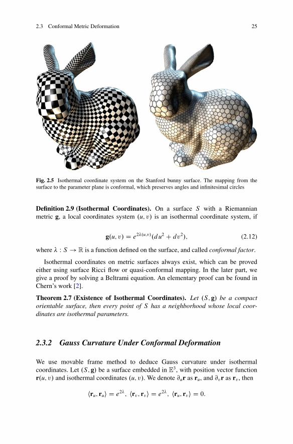
Fig. 2.5 Isothermal coordinate system on the Stanford bunny surface. The mapping from thesurface to the parameter plane is conformal, which preserves angles and infinitesimal circles
Definition 2.9 (Isothermal Coordinates). On a surface S with a Riemannianmetric g, a local coordinates system .u; v/ is an isothermal coordinate system, if
g.u; v/ D e2�.u;v/.du2 C dv2/; (2.12)
where � W S ! R is a function defined on the surface, and called conformal factor.
Isothermal coordinates on metric surfaces always exist, which can be provedeither using surface Ricci flow or quasi-conformal mapping. In the later part, wegive a proof by solving a Beltrami equation. An elementary proof can be found inChern’s work [2].
Theorem 2.7 (Existence of Isothermal Coordinates). Let .S; g/ be a compactorientable surface, then every point of S has a neighborhood whose local coor-dinates are isothermal parameters.
2.3.2 Gauss Curvature Under Conformal Deformation
We use movable frame method to deduce Gauss curvature under isothermalcoordinates. Let .S; g/ be a surface embedded in E
3, with position vector functionr.u; v/ and isothermal coordinates .u; v/. We denote @ur as ru, and @vr as rv , then
hru; rui D e2�; hrv; rvi D e2�; hru; rvi D 0:

26 2 Surface Topology and Geometry
Choose an orthonormal frame
e1 D e��ru; e2 D e��rv; e3 D n:
Then
dr D rudu C rvdv D e1e�du C e2e�dv D !1e1 C !2e2;
where !1 D e�du and !2 D e�dv. From (2.4), we get !12 D ��vdu C �udv.Therefore
d!12 D .�vv C �uu/du ^ dv D �K!1 ^ !2 D �Ke2�du ^ dv;then we obtain
K.u; v/ D �e�2�.u;v/�@2
@u2C @2
@v2
�� D ��g�; (2.13)
where the Laplace–Beltrami operator is
�g D e�2�.u;v/�@2
@u2C @2
@v2
�:
Let Ng be another Riemannian metric, conformal to the original metric,
Ng D e2�g;
where � is a scalar function. We choose isothermal coordinates for both g and Ng,then
g D e2�.du2 C dv2/; Ng D e2.�C�/.du2 C dv2/;
The Gauss curvature NK induced by Ng becomes
NK D �e�2.�C�/�.�C �/ D e�2� .�e�2��� � e�2���/ D e�2� .K ��g�/:
So we obtain the Yamabe equation
NK D e�2� .K ��g�/: (2.14)
2.3.3 Geodesic Curvature Under Conformal Deformation
Suppose C is a curve on the surface and the tangent direction ˛ of the curve has theangle � to the e1 direction. Then the geodesic curvature of C is
kg D d� C !12
ds:

2.3 Conformal Metric Deformation 27
Choose the isothermal coordinates .u; v/,
!12 D �vdu � �udv;
ds D e�pdu2 C dv2;
du
dsD e�� cos �;
dv
dsD e�� sin �;
kg D d�
dsC �vdu � �udv
dsD d�
ds� e��.�u sin � � �v cos �/
D d�
ds� hrg�;ni;
where rg D e���@@u ;
@@v
�, and n D .sin �;� cos �/ is the outward normal of the
curve on the tangent plane. The geodesic curvature can also be written as
kg D d�
ds� @n;g�:
Assume Ng is another Riemannian metric conformal to g, Ng D e2�g. Choose theisothermal coordinates .u; v/,
Ng D e2.�C�/.du2 C dv2/; g D e2�.du2 C dv2/;
then
Nkg D d�
d Ns � @n;Ng.�C �/:
Because d Ns D e�ds,
d�
d Ns D e��d�
ds:
Because rNg D e�����@@u ;
@@v
� D e��rg,
@n;Ng D hrNg;ni D e�� hrg;ni D e�� @n;g:
Therefore
Nkg D e��d�
ds� e�� @n;g.�C �/ D e��
�d�
ds� @n;g� � @n;g�
�D e�� .kg � @n;g�/:
Theorem 2.8 (Surface Yamabe Problem). Suppose S is a surface with aRiemannian metric g, which induces Gauss curvature K and geodesic curvature kgon the boundary. Let
Ng D e2�g
28 2 Surface Topology and Geometry
be another metric conformal to the original one, which induces Gauss curvatureNK and geodesic curvature Nkg. Then the changes of Gauss curvature and geodesic
curvature associated with the conformal metric change respectively are
NK D e�2�.K ��g�/;Nkg D e��.kg � @n;g�/:
Surface Yamabe problem is to find the conformal factor � from the prescribedcurvatures NK and Nkg, which can be solved using surface Ricci flow.
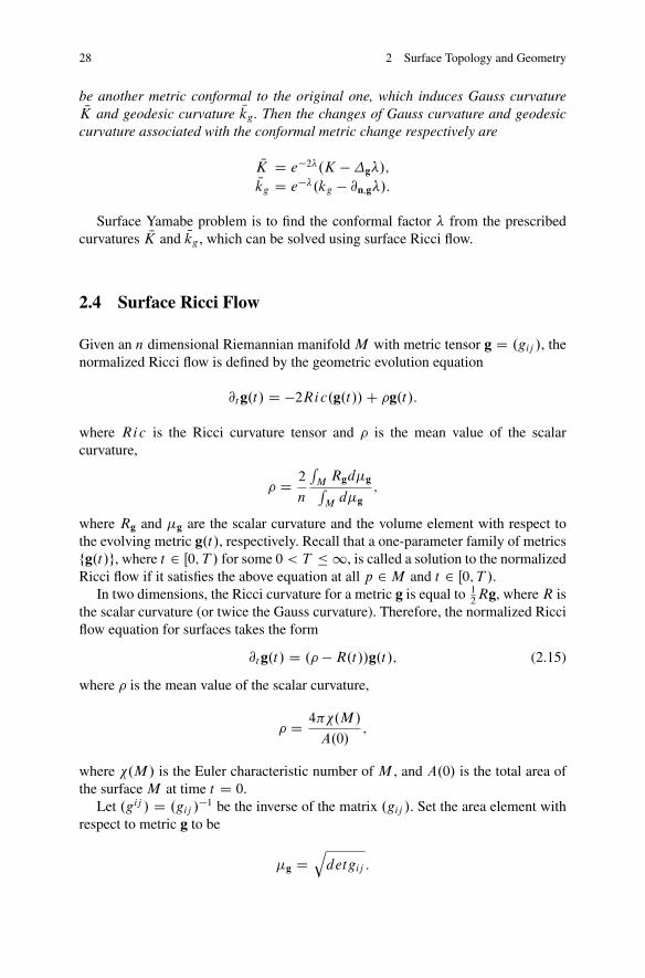
2.4 Surface Ricci Flow
Given an n dimensional Riemannian manifold M with metric tensor g D .gij /, thenormalized Ricci flow is defined by the geometric evolution equation
@tg.t/ D �2Ric.g.t//C g.t/:
where Ric is the Ricci curvature tensor and is the mean value of the scalarcurvature,
D 2
n
RMRgd�gRMd�g
;
where Rg and �g are the scalar curvature and the volume element with respect tothe evolving metric g.t/, respectively. Recall that a one-parameter family of metricsfg.t/g, where t 2 Œ0; T / for some 0 < T � 1, is called a solution to the normalizedRicci flow if it satisfies the above equation at all p 2 M and t 2 Œ0; T /.
In two dimensions, the Ricci curvature for a metric g is equal to 12Rg, where R is
the scalar curvature (or twice the Gauss curvature). Therefore, the normalized Ricciflow equation for surfaces takes the form
@tg.t/ D . �R.t//g.t/; (2.15)
where is the mean value of the scalar curvature,
D 4�.M/
A.0/;
where .M/ is the Euler characteristic number of M , and A.0/ is the total area ofthe surface M at time t D 0.
Let .gij / D .gij /�1 be the inverse of the matrix .gij /. Set the area element with
respect to metric g to be
�g Dqdetgij :

2.4 Surface Ricci Flow 29
Then along the Ricci flow, we compute
@t�g D 1
2gij @tgij �g D . �R/�g:
For the total area A D RMd�, we have
@tA.t/ DZM
. �R/d�g D 0:
Therefore, the normalized Ricci flow preserves the total area, A.t/ D A.0/;8t > 0.During the Ricci flow (2.15), the metric deforms conformally, g.t/ D e2�.t/g.0/,
@t� D 1
2. �R/; �.0/ D 0; (2.16)
and from Yamabe equation (2.14),
�0� � 1
2R0 C 1
2Re2� D �0� �K0 CKe2� D 0:
We obtain the curvature evolution equation
@tR D �g.t/RCR.R � /: (2.17)
Let u D e2�, then we get the evolution equation for u,
@tu D . �R/u:
Plug in R D u�1.R0 ��0 log u/, we get an evolution flow for u,
@tu D �0 log u C u �R0; u.0/ D u0: (2.18)
For most evolution equations, one proved that the solutions exist for all t 0 bycombining a short-time existence (and uniqueness) result with prior bounds whichshow that the solutions cannot develop singularities in finite time. Equation (2.18)is a parabolic equation. It can be set up as a fixed point problem for a contractionmapping. The mapping is obtained by applying the fundamental solution of thelinearization at any given u0 > 0 to (2.18); it is a contraction on any sufficientlyshort-time interval. This gives the proof for the short-time existence of the solution.The long-time existence can be obtained by estimating both the lower and upperbounds of R.t/ and u.t/, which requires a generalization of Li-Yau’s Harnackinequality [8]. The proofs require advanced background knowledge and sophisti-cated geometric skills, which is beyond the scope of the current book. Details canbe found in Hamilton’s [7] and Chow’s [4] works.

30 2 Surface Topology and Geometry
Theorem 2.9 (Hamilton [7]). Let .M2; g0/ be compact. If � 0, or if R.0/ 0
on all of M2, then the solution to (2.15) exists for all t 0 and converges to ametric of constant curvature.
Theorem 2.10 (Chow [4]). If g0 is any metric on S2, then its evolution under (2.15)
develops positive scalar curvature in finite time, and hence by Theorem 2.9converges to the round metric as t goes to 1.
In Chap. 4, we will give a discrete version of surface Ricci flow theory andprove its convergence (Theorem 4.6). Discrete surface Ricci flow shares thesame theoretical framework, the same fundamental principles, and even the sameformulae (comparing (2.16) and (4.10)), but only requires elementary geometricknowledge to prove. Furthermore, discrete surface Ricci flow theory leads to thepractical computational algorithms directly.
References
1. Armstrong, M.: Basic Topology. Undergraduate Texts in Mathematics. Springer, New York(1983)
2. Chern, S.: An elementary proof of the existence of isothermal parameters on a surface. Proc.Am. Math. Soc. 6(5), 771–782 (1955)
3. Chern, S.S., Cesari, L.: Global Differential Geometry. Mathematical Association of America,Providence, RI (1989)
4. Chow, B.: The Ricci flow on the 2-sphere. J. Differ. Geom. 33(2), 325–334 (1991)5. Chow, B., Lu, P., Ni, L.: Hamilton’s Ricci Flow, Graduate Studies in Mathematics, vol. 77.
American Mathematical Society, Providence, RI (2006)6. DoCarmo, M.P.: Differential Geometry of Curves and Surfaces, 1st edn. Pearson (1976)7. Hamilton, R.: Ricci flow on surfaces. Mathematics and General Relativity. Contemporary
Mathematics, vol. 71, pp. 237–261. AMS, Providence, RI (1988)8. Li, P., Yau, S.T.: On the parabolic kernel of the Schrödinger operator. Acta Math. 156, 153–201
(1986)9. Schoen, R., Yau, S.T.: Lecture on Differential Geometry, vol. 1. International Press Incorporated,
Boston (1994)

Chapter 3Riemann Surface
Riemann surface theory studies the invariants under conformal transformationgroup. This chapter briefly introduces the Riemann surface theory [7], includingquasi-conformal mapping [1], Teichmüller space [3,12], and surface harmonic maps[10, 11]. Finally, the Teichmüller theory of harmonic maps [13] is covered.
Surfaces are classified by conformal transformation group, and the space of allthe orbits is the Teichmüller space, which is a natural model for the shape space.General diffeomorphisms are quasi-conformal maps and can be represented bytheir Beltrami coefficients. The functional space of all Beltrami coefficients is anatural model for the mapping space. In order to obtain diffeomorphisms, harmonicmaps are often applied as the initial mappings, due to their simplicity and stability.Furthermore, under mild conditions, harmonic maps are diffeomorphic and uniquein their homotopy classes.
3.1 Conformal Structure
Definition 3.1 (Holomorphic Function). Suppose f W C ! C is a complexfunction, w D f .z/, in real form, f W x C iy ! u.x; y/C iv.x; y/. If f satisfiesthe Riemann–Cauchy equation
@u
@xD @v
@y;@u
@yD �@v
@x;
then f is a holomorphic function.
For convenience, we use complex differential operators,
d z D dx C idy; d Nz D dx � idy;
W. Zeng and X.D. Gu, Ricci Flow for Shape Analysis and Surface Registration,SpringerBriefs in Mathematics, DOI 10.1007/978-1-4614-8781-4__3,© Wei Zeng, Xianfeng David Gu 2013
31

32 3 Riemann Surface
Fig. 3.1 Biholomorphic functions are conformal mappings
@
@zD 1
2
�@
@x� i @
@y
�;@
@Nz D 1
2
�@
@xC i
@
@y
�:
If @f
@Nz D 0, then f is holomorphic.
Definition 3.2 (Biholomorphic Function). Suppose f W C ! C is invertible andboth f and f �1 are holomorphic. Then f is a biholomorphic function.
Let w D f .z/ be a biholomorphic function. The pullback metric induced byf W .C; jd zj2/ ! .C; jdwj2/ is
f �jdwj2 D jdwj2 D jwzd z C wNzd Nzj2 D jwzj2jd zj2:
Therefore, biholomorphic mappings are conformal diffeomorphisms. Figure 3.1shows a biholomorphic function. In the figure, we can see that the mappingpreserves local shapes, such as the decahedra and the paper bunny models.
Definition 3.3 (Conformal Atlas). Suppose S is a topological surface (two-dimensional manifold) and A is an atlas, such that all the chart transition functions�˛ˇ W C ! C are biholomorphic. Then A is called a conformal atlas.
Suppose S is a topological surface and A1, A2 are two conformal atlases. If theirunion A1 [ A2 is still a conformal atlas, then we say A1 and A2 are compatible,denoted as A1 � A2. The compatible relation among conformal atlases is anequivalence relation, which can classify all conformal atlases.
Definition 3.4 (Conformal Structure). Suppose S is a topological surface. Con-sider that all the conformal atlases on M are classified by the compatible relation,
fall conformal atlasesg= � :
Then each equivalence class is called a conformal structure.
3.2 Teichmüller Space 33
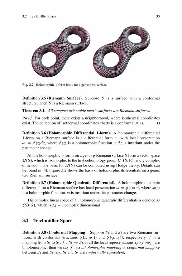
Fig. 3.2 Holomorphic 1-form basis for a genus two surface
Definition 3.5 (Riemann Surface). Suppose S is a surface with a conformalstructure. Then S is a Riemann surface.
Theorem 3.1. All compact orientable metric surfaces are Riemann surfaces.
Proof. For each point, there exists a neighborhood, where isothermal coordinatesexist. The collection of isothermal coordinates charts is a conformal atlas. ut
Definition 3.6 (Holomorphic Differential 1-form). A holomorphic differential1-form on a Riemann surface is a differential form !, with local presentation! D �.z/d z, where �.z/ is a holomorphic function. !d z is invariant under theparameter change.
All the holomorphic 1-forms on a genus g Riemann surface S form a vector space˝.S/, which is isomorphic to the first cohomology groupH1.S;R/, and g complexdimension. The basis for ˝.S/ can be computed using Hodge theory. Details canbe found in [4]. Figure 3.2 shows the basis of holomorphic differentials on a genustwo Riemann surface.
Definition 3.7 (Holomorphic Quadratic Differential). A holomorphic quadraticdifferential on a Riemann surface has local presentation ! D �.z/d z2, where �.z/is a holomorphic function. ! is invariant under the parameter change.
The complex linear space of all holomorphic quadratic differentials is denoted asQD.S/, which is 3g � 3 complex dimensional
3.2 Teichmüller Space
Definition 3.8 (Conformal Mapping). Suppose S1 and S2 are two Riemann sur-faces, with conformal structures f.U˛; �˛/g and f.Vˇ; �ˇ/g, respectively. f is amapping from S1 to S2, f W S1 ! S2. If all the local representations �ˇ ıf ı��1˛ arebiholomorphic, then we say f is a biholomorphic mapping or conformal mappingbetween S1 and S2, and S1 and S2 are conformally equivalent.

34 3 Riemann Surface
f
z wτβ ◦ f ◦ φα
−1
Uα
Vβ
φα τβ
S1 ⊂ {(Uα, φα)} S2 ⊂ {(Vβ, τβ)}
Fig. 3.3 Biholomorphic mapping (conformal mapping) between two Riemann surfaces. All �ˇ ıf ı ��1
˛ ’s are biholomorphic
Figure 3.3 illustrates a biholomorphic mapping between two Riemann surfaces.Suppose S is a compact orientable surface with genus g, and �g is the set of
all possible conformal structures on S . We say two elements �1; �2 2 �g areequivalent, denoted as �1 � �2, if there exists a conformal mapping f W S�1 !S�2 , where S�1 and S�2 are Riemann surfaces formed by S equipped with theconformal structures �1 and �2. The equivalence class of � 2 �g is denoted as Œ��.
Definition 3.9 (Moduli Space). The set of all equivalence classes Œ�� is called themoduli space of genus g Riemann surface, denoted as Rg ,
Rg D �g= � :
The topology of moduli space is complicated. In practice, Teichmüller space ismore preferred, which is the universal covering space of the moduli space.
Two conformal structures �1; �2 2 �g are Teichmüller equivalent, denoted as�1 �2, if there is a conformal mapping f W S�1 ! S�2 . Furthermore, treated asan automorphism of S , f W S ! S is homotopic to the identity.

3.3 Conformal Module 35
Definition 3.10 (Teichmüller Space). The set of Teichmüller equivalence classesin �g is called the Teichmüller space, denoted as T g,
T g D �g= :
3.3 Conformal Module
In this section, we apply surface Ricci flow to explain the concept of conformalmodule and analyze the dimension of the corresponding Teichmüller space. We useT .g;b/ to represent the Teichmüller space of surfaces of genus g with b boundarycomponents. The constructive proofs can be converted to computational methodsdirectly.
3.3.1 Topological Sphere
A topological sphere (a genus zero closed surface) can be conformally mapped tothe unit sphere. The mapping is not unique. Two such conformal mappings differ bya spherical Möbius transformation. Let � W S2 ! NC be the stereographic projection,which maps the unit sphere S
2 to the extended complex plane NC D C [ f1g,
�.x; y; z/ D�
x
1 � z;y
1 � z
�:
Let � be the Möbius transformation from the extended plane to itself,
�.z/ D az C b
cz C d; ad � bc D 1; a; b; c; d 2 C:
Then a spherical Möbius transformation has the form ��1 ı � ı �, which is 6dimensional. Therefore, all topological spheres are conformally equivalent; theTeichmüller space of all genus zero closed surfaces consists of a single point,T .0;0/ D fpg. Figure 3.4 shows an example, which can be computed using Ricciflow or the spherical harmonic map method. According to Theorem 3.9, harmonicmaps between genus zero closed surfaces are conformal.
3.3.2 Topological Quadrilateral
Suppose S is a genus zero surface with a single boundary and four marked boundarypoints, p1, p2, p3, p4, sorted counter-clockwisely. Then S is called a topologicalquadrilateral and denoted as Q.p1; p2; p3; p4/. There exists a unique conformalmap � W S ! C, such that � maps Q to a planar rectangle, �.p1/ D 0, �.p2/ D 1.

36 3 Riemann Surface
Fig. 3.4 Conformal mapping for a genus zero closed surface
Fig. 3.5 Conformal module for a topological quadrilateral. The face surface with four boundarycorners (a) is conformally mapped to a planar rectangle (b). A checkerboard texture is placedon the rectangle and pulled back to the face surface (c), all the right angles of checkers are wellpreserved
We can set the target Gauss curvature to be zero everywhere in the interior, andthe target geodesic curvature to be zero along the boundary, except at the fourcorners fp1; p2; p3; p4g. The target exterior angle for those four corners is �=2.Then Ricci flow produces a flat metric. By isometrically embedding the surface withthe flat metric onto the plane, we map it onto a planar rectangle, as shown in Fig. 3.5.The ratio between the height and the width of the rectangle is the conformal moduleof the topological quadrilateral. Therefore, the Teichmüller space for all topologicalquadrilaterals is one dimensional.
3.3.3 Topological Annulus
Suppose S is a topological annulus with a Riemannian metric g. The boundary of Sconsists of 2 loops, @S D �1 � �2. There exists a conformal mapping � W S ! C,which maps S to the canonical annulus, and �.�1/ and �.�2/ are concentric circles

3.3 Conformal Module 37
Fig. 3.6 Conformal module for a topological annulus. The face surface with two boundaries (a) isconformally mapped to a planar annulus (b). A checkerboard texture is placed on the annulus andpulled back to the face surface (c), all the right angles of checkers are well preserved
with radii r1 and r2 (r2 < r1), respectively, as shown in Fig. 3.6. The mapping �is unique up to a planar rotation. The conformal module is defined as Mod(S )D12�
ln r1r2
. Hence the Teichmüller space for all topological annuli is one dimensional,
dimT .0;2/ D 1.We can set the target Gauss curvature to be zero everywhere in the interior and
the geodesic curvatures along the boundaries to be zero everywhere. Then Ricciflow leads to a flat metric. We find a curve � connecting �1 and �2, such that � isa straight line segment under the flat metric and orthogonal to the two boundaries.We slice the surface along � to get QS , and � becomes two boundary segments �Cand ��. We then isometrically embed QS onto the plane. After a planar rigid motion,and a normalization, QS is a rectangle with the unit height, �� is on the real axis, and�1 is on the imaginary axis. Then we use the exponential map exp2�z to map QS to acanonical planar annulus.
3.3.4 Topological Disk
Suppose S is a topological disk with a Riemannian metric. Then it can beconformally mapped to the unit planar disk. Two such mappings differ by a Möbiustransformation
z ! ei�z � z01 � Nz0z ; (3.1)
as shown in Fig. 3.7. The Teichmüller space of topological disks consists of a singlepoint, T .0;1/ D fpg.
The computation is straightforward. We punch a small hole at the point z0 tomake the surface a topological annulus and map the annulus onto the canonicalplanar annulus. When the punched holes shrink to a point, the mappings convergeto the Riemann mapping.

38 3 Riemann Surface
Fig. 3.7 Riemann mappings for a topological disk. Two such mappings differ by a Möbiustransformation
3.3.5 Topological Multiply Connected Annulus
Suppose S is a genus zero surface with multiple boundaries. Then S is called atopological multiply connected annulus. Suppose S is with a Riemannian metric g.Then there exists a conformal mapping � W S ! C, which maps S to the unit diskwith circular holes (a planar circle domain). Such conformal mappings are uniqueup to Möbius transformations.
Let S be a multiply connected domain with nC 1 boundaries,
@S D �0 � �1 � �2 � � � � �n; (3.2)
where �0 is the exterior boundary and f�k; k > 0g are sorted by their total lengths.We set the target Gauss curvature to be zeros for all the interior points, and the targetgeodesic curvatures to be constant on each boundary, such that
Z�0
Nkg D 2�;
Z�i
Nkg D �2�; i > 0:
Ricci flow produces a conformal mapping, which maps the surface to the planarcircle domain. Let .xk; yk; rk/ represent the center and the radius of the circle imageof �k; k > 1. We can use a Möbius transformation to map the center of �1 to theorigin, and the center of �2 to be on the imaginary axis. Then the conformal moduleof the surface is given by
fr1; y2; r2; .x3; y3; r3/; � � � ; .xn; yn; rn/g:
So the dimension of the Teichmüller space of n-holed annuli is 3n � 3,dimT .0;nC1/ D 3n � 3. Figure 3.8 shows the canonical conformal mapping ofa multiply connected annulus, a partial surface of a 3D human face.

3.3 Conformal Module 39
Fig. 3.8 Conformal module for a topological multiply connected annulus. The face surface with16 boundaries (a) is conformally mapped to a planar circle domain (b). In the checkerboard texturemapping result (c), all the right angles of checkers are well preserved
3.3.6 Topological Torus
Given a topological torus (a genus one closed surface) S with a Riemannian metric,Ricci flow produces a flat metric. Then S is deformed to a flat torus T , and T canbe represented as the quotient space,
T D C=;
where is a lattice group,
D fz ! z CmC n!;m; n 2 Zg; ! 2 C; Img.!/ > 0:
! is the conformal module of the surface. Therefore, the Teichmüller space forgenus one surfaces is a two-dimensional manifold, dimT .1;0/ D 2. Figure 3.9 showsthe conformal module for a genus one closed surface.
3.3.7 Genus One Surface with Boundaries
We use the Ricci flow method to compute the canonical conformal mapping andthe conformal module. Suppose the boundary of the surface has n loops, @S D�1 C �2 C � � � C �n. We set the target Gauss curvature for all the interior points tobe zero the target geodesic curvature on each boundary to be constant, and the totalgeodesic curvature for each boundary loop is �2� ,
Z�k
Nkg D �2�; k D 1; 2; � � � ; n:

40 3 Riemann Surface
Fig. 3.9 Uniformization for genus one closed surface
Fig. 3.10 Uniformization for genus one surface with boundaries, Costa’s minimal surface
By running Ricci flow with the prescribed target curvature, a unique flat metric willbe obtained. The surface is isometrically mapped onto a flat torus with circular holes,
C= �n[
kD1Dk;
where fDkg are circles. The conformal module of the surface is given by thegenerators of the Lattice transformation group and the centers and radii of thecircular boundaries fDkg. The dimension of the Teichmüller space is given by
dimT.1;n/ D 2 C 3n:
Figure 3.10 shows the conformal module for a genus one surface with threeboundaries, Costa’s minimal surface [2].

3.3 Conformal Module 41
3.3.8 High Genus Closed Surface
Fuchs Group
Suppose S is a compact Riemann surface with genus g > 1. Let q0 2 S be the basepoint, select a set of canonical fundamental group generators fa1; b1; � � � ; ag; bgg,satisfying the following conditions
a1b1a�11 b�11 � � � agbga�1g b�1g � e: (3.3)
Suppose the universal covering of S is p W QS ! S , where p is the projection.Let z0 2 QS be one of the preimages of q0, z0 2 p�1.q0/. Through z0, lifta1; b1; a2; b2; � � � ; ag; bg to get paths,
Qa1; Qb1; Qa2; Qb2; � � � ; Qag; Qbg:
Suppose the end points of these curves are
�1; �1; �2; �2; � � � ; �g; �g:Then there must be 2g Deck transformations, ˛1; ˇ1; ˛2; ˇ2; � � � ; ˛g; ˇg , such that
˛j .z0/ D �j ; ˇj .z0/ D �j ; j D 1; 2; � � � ; g:
Because of (3.3), we obtain
˛1 ı ˇ1 ı ˛�11 ı ˇ�11 � � �˛g ı ˇg ı ˛�1g ı ˇ�1g D id: (3.4)
By Ricci flow, we can get the hyperbolic uniformization metric g of S , thenthe universal covering space QS , with the pullback metric p�g, can be isometricallyembedded in the hyperbolic space H
2. The Deck transformations are hyperbolicisometric transformations, and called Fuchsian transformations, and the Decktransformation group is called the Fuchs group of the surface.
Poincaré Model
We use the Poincaré disk model for the hyperbolic plane
H2 D fzj jzj < 1g; ds2 D 4d zd Nz
.1 � zNz/2 :
The hyperbolic lines through p and q are circular arcs passing through p and q,which are orthogonal to the unit circle. The hyperbolic circle .c; r/ on the Poincarédisk is identical to the Euclidean circle .C; R/, with the following relations,

42 3 Riemann Surface
C D 1 � t 21 � t 2cNcc; R D
sC NC � cNc � t 2
1 � t 2cNc ; t D tanhr
2; (3.5)
where c;C are the hyperbolic and Euclidean circle centers, respectively, and r; Rare the hyperbolic and Euclidean circle radii, respectively.
The Fuchsian transformations are Möbius transformations of hyperbolic type,
�.z/ D ei�z � z01 � Nz0z ; jz0j < 1; � 2 Œ0; 2�/;
which has two fixed points �.�/ D � and �.�/ D � on the unit circle. Let � be aMöbius transformation for the extended complex plane, which maps the fixed pointsto 0 and 1,
�.z/ D z � �z � � :
Then
� ı � ı ��1 W z ! kz; k ¤ 0; 1;
where k D � is a positive real number, which is called the multiplier of theMöbius transformation. Therefore, a hyperbolic type Möbius transformation canbe specified by its fixed points and multiplier .�; �; �/.
Fricke Coordinates
By (3.4), the Fuchs group generators ˛g; ˇg can be uniquely determined by ˛1,ˇ1, � � � , ˛g�1, ˇg�1, which in turn can be represented by their fixed points andmultipliers,
.�1; �1; �1; � � � ; �2g�2; �2g�2; �2g�2/:
This is called the Fricke coordinates of the Riemann surface in the Teichmüllerspace T g . So the Teichmüller space T g; g > 1 is 6g � 6 real dimensional,dimTg D 6g � 6.
Figure 3.11 shows the isometric embedding of the universal covering spaces oftwo high genus surfaces on the Poincaré disk with their uniformization hyperbolicmetrics.
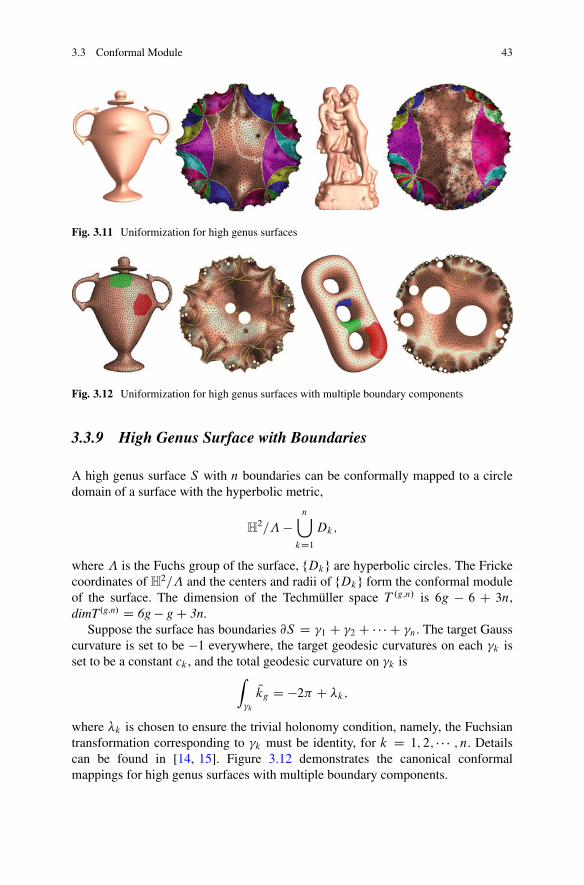
3.3 Conformal Module 43
Fig. 3.11 Uniformization for high genus surfaces
Fig. 3.12 Uniformization for high genus surfaces with multiple boundary components
3.3.9 High Genus Surface with Boundaries
A high genus surface S with n boundaries can be conformally mapped to a circledomain of a surface with the hyperbolic metric,
H2= �
n[kD1
Dk;
where is the Fuchs group of the surface, fDkg are hyperbolic circles. The Frickecoordinates of H2= and the centers and radii of fDkg form the conformal moduleof the surface. The dimension of the Techmüller space T .g;n/ is 6g � 6 C 3n,dimT.g;n/ D 6g � g C 3n.
Suppose the surface has boundaries @S D �1 C �2 C � � � C �n. The target Gausscurvature is set to be �1 everywhere, the target geodesic curvatures on each �k isset to be a constant ck , and the total geodesic curvature on �k isZ
�k
Nkg D �2� C �k;
where �k is chosen to ensure the trivial holonomy condition, namely, the Fuchsiantransformation corresponding to �k must be identity, for k D 1; 2; � � � ; n. Detailscan be found in [14, 15]. Figure 3.12 demonstrates the canonical conformalmappings for high genus surfaces with multiple boundary components.

44 3 Riemann Surface
3.4 Quasi-Conformal Mapping
General diffeomorphisms between compact surfaces are rarely conformal, but arequasi-conformal. Geometrically, a conformal mapping maps infinitesimal circlesto infinitesimal circles, whereas, a quasi-conformal mapping maps infinitesimalellipses to infinitesimal circles. Figure 3.13 demonstrates both a conformal mappingand a quasi-conformal mapping from a 3D human face surface to the unit disk.We put the circle packing texture on the unit disk, and pull it back to the 3D facesurface by the mapping. In the left two frames, the mapping is conformal, therefore,the circles are pulled back to circles; in the right two frames, the mapping is quasi-conformal, and the circles are pulled back to ellipses.
3.4.1 Measurable Riemann Mapping
We first consider planar mappings. Suppose D is a domain on the complex planeand f W D ! C is a differentiable mapping, f W .x; y/ ! .u; v/. For convenience,we use complex representations: z D x C iy, w D u C iv, and w D f .z/. Then themapping can be locally approximated by an affine transformation,
df D @f
@zd z C @f
@Nz d Nz: (3.6)
If f is holomorphic, then @f=@Nz D 0. The Jacobian of the mapping is given by
J Dˇˇ@f@z
ˇˇ2
�ˇˇ@f@Nz
ˇˇ2
:
If f is a diffeomorphism, then
ˇˇ@f@Nzˇˇ <
ˇˇ@f@z
ˇˇ : (3.7)
Fig. 3.13 Solving Beltrami equation using the auxiliary metric method. (a–b) A conformalmapping and its induced circle packing texture mapping for the � � 0, (c–d) A quasi-conformalmapping and its induced circle packing texture mapping for a given �

3.4 Quasi-Conformal Mapping 45
It follows from (3.6) that
.jfzj � jfNzj/jd zj � jdwj � .jfzj C jfNzj/jd zj;
where both limits can be attained. At the point z, the mapping maps an infinitesimalcircle to an infinitesimal ellipse, and the ratio of the major axis to the minor axis is
Kf D jfzj C jfNzjjfzj � jfNzj 1:
This is called the dilatation at the point z. It is often more convenient to consider
kf D jfNzjjfzj < 1;
related to Kf by
Kf D 1C kf
1 � kf ; kf D Kf � 1Kf C 1
:
Definition 3.11 (Beltrami Coefficient). We introduce the complex dilatation orthe Beltrami coefficient of the mapping f ,
�f D fNzfz;
with j�f j D kf .
The direction of the major axis of the ellipse corresponds to the direction
arg d z D ˛ D 1
2arg�:
The minor axis direction is ˛ ˙ �=2.
Definition 3.12 (Quasi-Conformal Mapping). The mapping f is said to be quasi-conformal if Kf is bounded. It is K-quasi-conformal if Kf � K.
The condition Kf � K is equivalent to kf � .Kf � 1/=.Kf C 1/. A 1-quasi-conformal mapping is conformal.
Suppose f W D ! G and g W D1 ! G1 are two quasi-conformal mappings, andG � D1. Then the Beltrami coefficient for the composition g ı f is given by
�gıf D �f C .�g ı f /�1C N�f � .�g ı f /� ; � D Nfz=fz:

46 3 Riemann Surface
Similarly, suppose f W D ! G and g W D ! G0 are quasi-conformal mappingswith Beltrami coefficients �f and �g, respectively. Then the Beltrami coefficientg ı f �1 W G ! G0 is given by
�gıf �1 .f / D �g � �f1 � N�f �g � ��1; � D Nfz=fz:
If f W D ! D is a quasi-conformal mapping with Beltrami coefficient �f , thenk�f k1 < 1; the inverse is also true.
Theorem 3.2 (Measurable Riemann Mapping). Suppose ˝ is a simply con-nected domain in C, ˝ � C, which has more than one boundary point. Assume�.z/ is a bounded measurable function defined in the interior of ˝ and k�k1 < 1,then there exists a homeomorphism f W ˝ ! D, which maps ˝ to the unit disk,furthermore f satisfies the Beltrami equation
@f
@Nz D �.z/@f
@z: (3.8)
Two such mappings f1; f2 W ˝ ! D, differ by a Möbius transformation, namely,f2 ı f �11 W D ! D has the following representation
f2 ı f �11 .z/ D ei�z � z01 � Nz0z ; jz0j < 1; � 2 Œ0; 2�/:
Proof. We give a brief geometric proof based on the Auxiliary Metric Method. Letf W ˝ ! D be the quasi-conformal with the Beltrami coefficient �, then
f W .˝; d zd Nz/ ! .D; dwd Nw/
is quasi-conformal. Consider the same map f with a different Riemannian metric,and the pullback metric induced by f , f �dwd Nw D dwd Nw, then
f W .˝; dwd Nw/ ! .D; dwd Nw/
is isometric. The pullback metric
dwd Nw D jwzd z C wNzd Nzj2 D jwzj2ˇˇd z C wNz
wzd Nzˇˇ2 D jwzj2jd z C �f d Nzj2
is conformal to an auxiliary metric
Qg WD jd z C �d Nzj2: (3.9)
Then the same mapping f under the auxiliary metric
f W .˝; jd z C �d Nzj2/ ! .D; dwd Nw/

3.4 Quasi-Conformal Mapping 47
is a conformal mapping. According to Riemann mapping theorem, the conformalmapping f under the auxiliary metric exists and is unique up to a Möbiustransformation. ut
Although the proof is for topological disk, it can be directly generalized tocompact Riemann surfaces with arbitrary topologies, where the concept of Beltramicoefficient �f D fNz=fz needs to be replaced by the concept of Beltrami differential.
Definition 3.13 (Beltrami Differential). Suppose f W S1 ! S2 is a diffeo-morphism between two Riemann surfaces S1 and S2. Suppose z and w are localconformal parameters of S1 and S2, respectively, and f has the local representationw D f .z/. Then the Beltrami differential of f has the local representation
�f WD fNzfz
d Nzd z:
We can solve Beltrami equations (3.8) on surfaces with complicated topologiesusing Ricci flow combined with the auxiliary metric method. Figure 3.13 shows thecomputational results for multiply connected annulus surfaces.
3.4.2 Existence of Isothermal Coordinates
The measurable Riemann mapping theorem leads to the existence of isothermalcoordinates.
Corollary 3.1 (Isothermal Coordinates). Let S be a smooth metric surface. Forany point p 2 S , there exists a neighborhood U.p/. The isothermal coordinatesexist on U.p/.
Proof. Suppose S is with a Riemannian metric
g.x; y/D�g11 g12g21 g22
�D�
cos � sin �� sin � cos �
���1 0
0 �2
��cos � � sin �sin � cos �
�; �1 > �2 > 0:
Choose a neighborhood U.p/, define Beltrami coefficient
�.z/ D �1 � �2�1 C �2
ei2� ; z D x C iy;
and solve the Beltrami equation wNz D �.z/wz, where w D uC iv. Because k�k1 <
1, the equation has a solution (k�k1 is the maximum of the norm of � on S ). Then.u; v/ are the isothermal coordinates of the surface. ut

48 3 Riemann Surface
3.4.3 Conformal Surface Representation
In order to represent a parametric surface embedded in E3, generally, we need three
functions, r.u; v/ D .x.u; v/; y.u; v/; z.u; v//, to represent its position. In fact, byusing isothermal coordinates, only two functions are sufficient.
Theorem 3.3. A closed surface embedded in E3 with isothermal coordinates .u; v/
is determined by the conformal factor �.u; v/ and the mean curvature H.u; v/uniquely up to a rigid motion. A simply connected surface with a boundary isdetermined by the conformal factor, the mean curvature and the boundary position.
Proof. Because z D u C iv is isothermal, we have
�2 D hru; rui D hrv; rvi;
hru; rvi D 0:
This is equivalent to
hrz; rzi D 0; hrNz; rNzi D 0; hrz; rNzi D �2
2:
The natural frame of the surface is given by frz; rNz;ng, where n is the normal fieldof the surface. Let
� D hrzz;ni;then the motion equation for the natural frame can be formulated as
rzz D 2��zrz C �n;
rzNz D �2
2Hn;
nz D �Hrz � 2�2�rNz;
(3.10)
with Gauss equation (3.11) and Codazzi equation (3.12)
.log�/zNz D � N��2
� �2
4H2; (3.11)
�Nz D �2
2Hz: (3.12)
The Codazzi equation is equivalent to the following Poisson problem
�zNz D 1
2�.2�zHz C �Hzz/:
One can solve � from this Poisson equation, then integrate the natural framefrz; rNz;ng to reconstruct the surface. This completes the proof. ut

3.4 Quasi-Conformal Mapping 49
Corollary 3.2. Given a closed surface embedded in E3 with isothermal coordinates
(conformal structure), if the two principle curvatures k1.u; v/ and k2.u; v/ areknown, then the surface can be determined uniquely up to a rigid motion of E3.
Proof. From the Gauss curvature K D k1k2 and the conformal structure, one cancompute the conformal factor � using Ricci flow. Combined with the mean curvatureH D .k1 C k2/=2, the surface can be determined uniquely up to a rigid motion. ut
3.4.4 Diffeomorphism Space and Beltrami Holomorphic Flow
Suppose metric surfaces .S1; g1/ and .S2; g2/ are two topological disks. Consider thespace of all diffeomorphisms between them and the space of Beltrami coefficients.From measurable Riemann mapping theorem, we obtain the following relation
fDiffeomorphismsgfMöbiusg Š fBeltrami Coefficientsg:
In what follows, f � will always denote the solution to the Beltrami equation on theextended complex plane NC D C [ f1g with fixed points 0; 1;1. Let
R.z; �/ D 1
z � � � �
1 � zC � � 1
z:
Suppose
�.t C s/.z/ D �.t/.z/C s�.t/.z/C s�.s; t/.z/;
where
�.t/; �.t/; �.s; t/ 2 L1; k�.t/k1 < 1;
and k�.s; t/k1 ! 0 as s ! 0, where k�.s; t/k1 is defined as supz2 NC k�.s; t/.z/k.Then
f �.tCs/.�/ D f �.t/.�/C s Pf .�; t/C o.s/
uniformly on compact sets, where
Pf .�; t/ D � 1�
Z Z�.t/.z/R.f �.t/.z/; f �.t/.�//.f �.t/
z .z//2dxdy: (3.13)
This formula gives the dependence of the mapping on the Beltrami coefficients.Besides the auxiliary metric method, this variation formula gives a different way tosolve Beltrami equations fNz D �fz. We define a homotopy �.t/ D t�; t 2 Œ0; 1�.Obviously, f �.0/ is a conformal mapping. Then we use the above formula to deform

50 3 Riemann Surface
the mapping from f �.0/ to f �.1/. This method is called the Beltrami holomorphicflow method [8].
Furthermore, this formula can be applied for many optimization problems in thediffeomorphism space.
3.4.5 Teichmüller Map and Teichmüller Distance
Let �.z/d z2 be a holomorphic quadratic differential on a Riemann surface S . Letp be a regular point, such that �.p/ ¤ 0. Then we can choose a neighborhoodU.p/ D fz; jz �pj < rg of p, such that � is nonzero inside U.p/. Then choose onebranch of
p�.z/, and define
�.z/ DZ z
0
p�.t/dt;
the mapping z ! � is biholomorphic, and � is called the natural parameter inducedby �.
Definition 3.14 (Teichmüller Map). Let S0 and S1 be two Riemann surfaces andf W S0 ! S1 be a quasi-conformal map. Suppose !0 and !1 are holomorphicquadratic differentials on S0 and S1, respectively. If f maps the regular points of!0 to the regular points of !1 and the zeros of !0 to the zeros of !1 with the sameorders, and let �0 and �1 be the natural parameters induced by !0 and !1, f has thelocal representation
f W �0 ! �1 D K C 1
2�0 C K � 1
2N�0;
where K 1 is a constant, then we call f a Teichmüller map, !0 the source holo-morphic quadratic differential, and !1 the target holomorphic quadratic differential.
The followings are the fundamental theorems in Teichmüller theory.
Theorem 3.4 (Existence of Teichmüller Map). Suppose S0 and S1 are twoRiemann surfaces with genus g > 1. If f W S0 ! S1 is an orientation preservinghomeomorphism, then there exists a Teichmüller map homotopic to f .
Theorem 3.5 (Uniqueness of Teichmüller Map). Suppose S0 and S1 are twoRiemann surfaces with genus g > 1. If f0 W S0 ! S1 is a Teichmüller map, then forany map f W S0 ! S1 homotopic to f0,
KŒf � KŒf0�;
and the equality holds if and only if f D f0.
Teichmüller map gives a Riemannian metric for the Teichmüller space.

3.5 Harmonic Maps 51
Definition 3.15 (Teichmüller Distance). Suppose S is a topological surface, and�1 and �2 are two conformal structures on S . S�1; S�2 2 T g are two Riemannsurfaces. The Teichmüller distance between the two Riemann surfaces is given by
dT .S�1; S�2/ D inff�id logKŒf �:
Then the dilatation of Teichmüller map between S�1 and S�2 gives the distance.The Teichmüller space under the Teichmüller distance is a Riemannian manifold.
Theorem 3.6. The Teichmüller space T g, g 1 with the Teichmüller distance dTis a Riemannian manifold .T g; dT /.
3.5 Harmonic Maps
Harmonic maps are the natural generalizations of geodesics, which have beenbroadly applied for computing the diffeomorphisms among surfaces. In the follow-ing discussion, we always use isothermal coordinates, unless otherwise specified.
Suppose a map w W .M; � jd zj2/ ! .N; jdwj2/ is given. If for any two pointsp; q 2 M ,
d .w.p/;w.q// < Kd�.p; q/;
where K is a positive constant, then the map is a Lipschitz map. The energy densityat a point z is defined to be
e.wI �; / D .w.z//
�.z/jwzj2 C .w.z//
�.z/jwNzj2:
The harmonic energy of the map is defined to be
E.wI �; / DZM
e.wI �; /�d zd Nz:
The total energy depends on the metric of the target surface and the conformalstructure of the source surface.
Definition 3.16 (Harmonic Map). A Lipschitz map w W .M; � jd zj2/ !.N; jdwj2/ is called a harmonic map if it is a critical point of the energy functionalE.wI �; / in the mapping space.
The Euler–Lagrange equation for the energy functional is
wzNz C .log /wwzwNz D 0: (3.14)

52 3 Riemann Surface
Given an initial mapping, the heat flow method,
@w
@tD �wzNz � .log /wwzwNz;
can deform it to a harmonic map.
3.5.1 Topological Disk
Suppose a harmonic mapping is from a topological disk to a planar disk. If therestriction on the boundary is a homeomorphism, then the map is a diffeomorphism.
Theorem 3.7 (Radó [11]). Assume ˝ � E2 is a convex domain with a smooth
boundary @˝ and a metric surface .S; g/ is a simply connected domain with asingle boundary. Given any homeomorphism � W @S ! @˝, then the harmonicmap u W S ! ˝, such that u D � on @S , is a diffeomorphism.
Proof. We can map S conformally onto the planar disk D by a Riemann mapping� W S ! D, then the composition � ı ��1 W D ! ˝ is still harmonic. We denotethe map as w.z/, or in real form .u.x; y/; v.x; y//. Then both u and v are harmonicfunctions,
�u � 0; �v � 0:
Suppose at one interior point p, the Jacobian is degenerated. Then there are two realnumbers .�1; �2/ ¤ .0; 0/, such that
�1ru C �2rv D 0:
Define a linear function f W ˝ ! R, f .u; v/ D �1u C �2v, then
f .x; y/ D �1u.x; y/C �2v.x; y/
is a harmonic function defined on D, with an interior singularity p. Because f isharmonic, p cannot be local maximum or minimum, then p must be a saddle point.Therefore the level set f D f .p/C � has two branches and intersects the boundaryof D at four points fz1; z2; z3; z4g. But each line �1u C �2v D const has only twointersection points fw1;w2g with @˝, because ˝ is convex. Therefore, the mappingw.z/maps four points fzig to the two points fwj g, so the mapping � restricted on theboundary @S to @˝ is not a homeomorphism. This contradicts the assumption that� W @S ! @˝ is a homeomorphsim. Therefore, the Jacobian is nonzero everywherein the interior of the surface, namely, the mapping is a diffeomorphism. ut
Furthermore, the harmonic map is unique.

3.5 Harmonic Maps 53
Fig. 3.14 Harmonic map for a human face surface
Theorem 3.8. Assume ˝ � E2 is a simply connected domain with a smooth
boundary @˝ and a metric surface .S; g/ is simply connected with a singleboundary. Given any homeomorphism � W @S ! @˝, if there exists a harmonicmap u W S ! ˝, such that u D � on @S , then u is unique.
Proof. The uniqueness of harmonic maps between topological disks can be easilyshown using the mean value property. By using Riemann mapping, the harmonicmapping between two metric surfaces which are topological disks is converted toa harmonic mapping from the unit disk to itself, w.z/ D .u.x; y/; v.x; y//, whereu; v are harmonic functions �
wzNz � 0
wj@D D w0:
From Poisson’s formula
w.rei�/ D 1
2�
Z 2�
0
w0.ei� /
1 � r21 � 2r cos.� � �/C r2
d�;
we get the mean value property. Namely, for any interior point z0 2 D, one canchoose a small circle surrounding z0, z0 C �ei� ,
w.z0/ D 1
2��
Z 2�
0
w.z0 C �ei� /d�;
therefore, the maximum and the minimum of u and v must be on the boundary ofthe unit disk.
Suppose there are two harmonic mappings w1;w2 W D ! D with the sameboundary conditions w0 W @D ! @D. Then the maximum and the minimum of theharmonic function u1 � u2 are on the boundary, therefore 0’s, so u1 � u2. Similarly,v1 � v2, therefore w1 � w2. ut
Figure 3.14 shows an example for a harmonic map from a human face surfaceonto the planar disk. From example, one can see that the harmonic map is close to

54 3 Riemann Surface
be conformal and introduces relatively small angle distortions. In fact, conformalmappings are harmonic, but harmonic maps may not necessarily be conformal.In the figure, if we only fix the images of 3 boundary points, and allow the boundaryimages �.p/, p 2 @S to slide along @D, and further minimize harmonic energy, thenwhen the energy reaches the minimum, we obtain a unique conformal mapping.
3.5.2 Genus Zero Closed Surface
The following discussion follows the proof in [9].Consider the pullback of the metric by the map w,
w� D dwd Nw D wzwNzd z2 C . jwzj2 C jwNzj2/d zd Nz C wzwNzd Nz2:
The Hopf differential is defined to be the .2; 0/ part of this pullback,
˚.w/ D wzwNzd z2:
When w is harmonic, the Hopf differential ˚.w/ is holomorphic. If w is conformal,then ˚.w/ vanishes. Hence we get the following,
Proposition 3.1. Suppose w is an orientation preserving diffeomorphism. If w isharmonic, then the Hopf differential ˚.w/ is holomorphic. If w is conformal, then˚.w/ vanishes.
Proof. Take the partial derivative of Hopf differential �.z/,
�.z/Nz D . wwNzwz C wzNz/wNz C . Nw. Nw/NzwNz C .wNz/Nz/wz:
The first term is zero, due to (3.14). Because wNz D . Nw/z, the second term is
. Nw. Nw/Nz. Nw/z C . Nw/zNz/wz;
which is also zero. Therefore, if w is harmonic, then its Hopf differential is a holo-morphic quadratic differential. If w is an orientation preserving diffeomorphism,then its Jacobian is jwzj2 � jw Nwj2 > 0. �.z/ D wzwNz vanishes if and only if wNz D 0,namely, w is conformal. utTheorem 3.9. Harmonic maps between genus zero closed metric surfaces areconformal.
Proof. Suppose w is harmonic. Then its Hopf differential ˚.w/ is a holomorphicquadratic differential. On genus zero closed metric surfaces, holomorphic quadraticdifferentials vanish, therefore, w is conformal. ut

3.5 Harmonic Maps 55
3.5.3 High Genus Closed Surface
In the following, we show that if the target surface has negative curvature every-where, then degree one harmonic map is diffeomorphic. We follow the proof in [9].More details can also be found in [10, 11].
We can define the auxiliary functions,
H D .w.z//�.z/ jwzj2;
L D .w.z//�.z/ jwNzj2:
The Jacobian of the mapping J is given by
J D H � L :
The complex form of the Laplace–Beltrami operator on .M; � jd zj2/ is
�� D 4
�
@2
@z@Nz ;
then the Gauss curvatures are given by
K.�/ D �12�� log �; K. / D �1
2� log :
This gives the Bochner formula,
�� log H D �2K. /H C 2K. /L C 2K.�/ D �2K. /J C 2K.�/;
�� log L D �2K. /L C 2K. /H C 2K.�/ D 2K. /J C 2K.�/:
The difference between these two equations gives the relation between the Jacobianof the map and the Gauss curvature on the target surface,
�� logH
LD �4K. /J :
In case M and N are compact surfaces of genus gM and gN , respectively, w WM ! N is a harmonic map of degree deg.w/, then the function H either vanishesidentically or has at most isolated zeros. Each zero point p 2 M has an ordernp 2 Z; np 0, and the summation of the orders of all zero points is
XH .p/D0
np D �deg.w/.4gN � 4/C .4gM � 4/: (3.15)
Similarly, if L is not identically zero, then
XL .p/D0
np D deg.w/.4gN � 4/C .4gM � 4/:

56 3 Riemann Surface
Suppose J is not identically zero, and p 2 M is a zero point of J , J .p/ D 0,then one can show H .p/ D 0 and L .p/ D 0. Therefore, the zero points of Jmust be isolated. If J 0 everywhere, and the number of preimages fw�1.q/g ofa regular value q 2 N is bounded, then the zero of J is a nontrivial branch pointof w.
Theorem 3.10. If the metric surface .M; � jd zj2/ and .N; jdwj2/ have the samegenus g 1, and the Gauss curvatureK. / on the target is nonpositive everywhere,K. / � 0, then a degree 1 harmonic map w W M ! N must be a diffeomorphism.
Proof. First, we claim J 0 everywhere. Otherwise, assume at a point p 2 M ,J < 0. We can define a region D � M ,
D D fq 2 M jJ .q/ < 0g;
Because p 2 D, D is nonempty. In the region D [ @D, J � 0,
�� logH
LD �2K. /J � 0;
so log HL is superharmonic. From formula (3.15), the total order of zeros of H is
XH .p/D0
np D 0;
therefore H has no zeros, and H > 0 everywhere. On the boundary ofD, p 2 @D,
J .p/ D H � L D 0; logH
LD 0;
so L .p/ > 0. For any interior point q 2 D, log HL is no less than the boundary
value 0, therefore
logH
L 0; H L ;
hence J D H �L 0 in the wholeD. This contradicts the assumption J .p/ <
0, p 2 D. Therefore, J 0 everywhere.From the above discussion, J has at most isolated zeros which are nontrivial
branch points. Since the degree of the map is 1, these zeros do not exist, so we haveJ > 0 on M and w is a diffeomorphism. ut
Furthermore, if the target surface is of genus g > 1 and the Gauss curvature isnonpositive, then the degree one harmonic map exists [6] and is unique [5].

References 57
3.5.4 Teichmüller Space Representation
Finally, we show that the space of all holomorphic quadratic differentials ˚d z2 on.M; � jd zj2/, denoted as QD.�/, has one-to-one correspondence to the Teichmüllerspace T g, where T g is represented as all possible hyperbolic metrics on N ,.N; jdwj2/.Theorem 3.11. Suppose w W .M; � jd zj2/ ! .N; jdwj2/ where K.�/ � �1,K. / � �1, and w is harmonic. The Hopf differential ˚ induces a map from thespace of holomorphic quadratic differentials QD.�/ to the Teichmüller space T g.˚ is injective.
Proof. Suppose there are two harmonic maps w1;w2 from .M; � jd zj2/ to.N; 1jdwj2/ and .N; 2jdwj2/, respectively, where K. 1/ � �1 and K. 2/ � �1,and they induce the same Hopf differential ˚1 D ˚2 D ˚ . Then for h D log H ,
�h D 2eh � 2j˚ j2e�h � 2:
If h1 > h2 somewhere, then we can look at a maximum of h1 � h2 and find that
0 �.h1 � h2/ D .eh1 � eh2/ � j˚ j2.e�h1 � e�h2/ > 0;
so h1 � h2. Symmetrically, h2 � h1, so h1 D h2 everywhere. Then H1 D H2.Since H1L1 D j˚ j2 D H2L2 and Hk > 0, we obtain L1 D L2. Consequently,the densities ek D Hk C Lk , k D 1; 2 are equal. Therefore, the pullback metrics
w�k D ˚kd z2 C �ekd zd Nz C Nkd Nz2; k D 1; 2;
are equal so that w1ıw�12 W .N; 2/ ! .N; 1/ is an isometry isotopic to the identity.ut
Therefore, holomorphic quadratic differentials can be treated as the tangent spaceof the Teichmüller space.
References
1. Ahlfors, L.V.: Lectures on Quasiconformal Mappings. University Lecture Series, vol. 38, 2ndedn. American Mathematical Society, Providence, RI (2006). With supplemental chapters byC. J. Earle, I. Kra, M. Shishikura and J. H. Hubbard
2. Costa, C.: Example of a complete minimal immersion in R3 of genus one and three embedded
ends. Bull. Soc. Bras. Mat. 15, 47–54 (1984)3. Gardiner, F., Lakic, N.: Quasiconformal Teichmüler Theory. American Mathematical Society,
Providence, RI (1999)4. Gu, X.D., Yau, S.T.: Computational Conformal Geometry. Advanced Lectures in Mathematics.
High Education Press and International Press, Somerville (2008)

58 3 Riemann Surface
5. Hartman, P.: On homotopic harmonic maps. Can. Math. Soc. 19, 673–687 (1967)6. James Eells, J., Sampson, J.H.: Harmonic mappings of riemannian manifolds. Am. J. Math.
86(1), 109–160 (1964)7. Jost, J.: Compact Riemann Surfaces: An Introduction to Contemporary Mathematics. Univer-
sititext. Springer, Berlin (1997)8. Lui, L.M., Wong, T.W., Zeng, W., Gu, X., Thompson, P.M., Chan, T.F., Yau, S.T.: Optimization
of surface registrations using Beltrami holomorphic flow. J. Sci. Comput. 50(3), 557–585(2012)
9. Schoen, R., Yau, S.T.: On univalent harmonic maps between surfaces. Invent. Math. 44(3),265–278 (1978)
10. Schoen, R., Yau, S.T.: Lecture on Differential Geometry, vol. 1. International Press Incorpo-rated, Boston (1994)
11. Schoen, R., Yau, S.T.: Lecture on Harmonic Maps, vol. 2. International Press Incorporated,Boston (1997)
12. Seppala, M., Sorvali, T.: Geometry of Riemann Surfaces and Teichmüller Spaces. North-Holland Mathematics Studies. North-Holland Publishing, Amsterdam (1992)
13. Wolf, M.: The Teichmüller theory of harmonic maps. J. Differ. Geom. 29(2), 449–479 (1989)14. Zeng, W., Yin, X., Zhang, M., Luo, F., Gu, X.: Generalized Koebe’s method for conformal
mapping multiply connected domains. In: ACM Symposium on Solid and Physical Modeling(SPM’09), pp. 89–100, ACM, New York, NY, 2009
15. Zhang, M., Li, Y., Zeng, W., Yau, S.T., Gu, X.: Canonical conformal mapping for high genussurfaces with boundaries. Int. J. Comput. Graph. 36(5), 417–426 (2012)

Chapter 4Discrete Surface Ricci Flow
This chapter systematically introduces the discrete surface Ricci flow theory. Thewhole theory is explained using the variational principle on discrete surfaces basedon derivative cosine law [18].
Ricci flow conformally deforms the Riemannian metrics, such that during theflow the infinitesimal circles are preserved. This phenomenon inspired Thurston todevelop the circle packing method. In his work on constructing hyperbolic metricson 3-manifolds, Thurston [25] studied a Euclidean (or a hyperbolic) circle packingon a triangulated closed surface with prescribed intersection angles. His workgeneralizes Koebe’s and Andreev’s results of circle packing on a sphere [1, 2, 14].Thurston conjectured that the discrete conformal mapping based on circle packingconverges to the smooth Riemann mapping when the discrete tessellation becomesfiner and finer. Thurston’s conjecture has been proved by Rodin and Sullivan [21].Chow and Luo established the intrinsic connection between circle packing andsurface Ricci flow [6].
4.1 Discrete Surface
In practice, smooth surfaces are usually approximated by discrete surfaces, namely,triangular meshes. Figure 4.2 demonstrates such an example. The surface of thesculpture of Michelangelo’s David is approximated by a triangular mesh. Eachface of the mesh is a Euclidean triangle. With high sampling density, the discretesurface can approximate the smooth surface accurately.
The combinatorial structure of a discrete surface is represented by a simplicialcomplex. The fundamental concepts from smooth differential geometry, such asRiemannian metric, curvature and conformal structure, are generalized to thesimplicial complex, respectively.
W. Zeng and X.D. Gu, Ricci Flow for Shape Analysis and Surface Registration,SpringerBriefs in Mathematics, DOI 10.1007/978-1-4614-8781-4__4,© Wei Zeng, Xianfeng David Gu 2013
59

60 4 Discrete Surface Ricci Flow
Fig. 4.1 A non-manifoldsimplicial complex
4.1.1 Simplicial Complex
Definition 4.1 (Simplex). Suppose n C 1 points fv0; v1; : : : ; vng in the generalpositions in R
n. The standard simplex Œv0; v1; : : : ; vn� is the minimal convex set
� D Œv0; v1; : : : ; vn� WD(
nXiD0
�ivi jnXiD0
�i D 1; �i 0
):
We call v0; v1; : : : ; vn the vertices of the simplex � .
Definition 4.2 (Facet). Suppose � is a simplex, and � � � is also a simplex. Thenwe say � is a facet of � .
The simplex has an orientation. Suppose .i0; i1; : : : ; in/ is a permutation of.0; 1; : : : ; n/. Œvi0 ; vi1 ; : : : ; vin � has the same orientation as Œv0; v1; : : : ; vn� if thepermutation is the product of even number of swaps. Otherwise, they have oppositeorientations if the permutation can be decomposed to odd number of swaps.
Definition 4.3 (Boundary Operator). The boundary of a simplex � is
@� DnXiD0.�1/j Œv0; : : : ; vj�1; vjC1; : : : ; vn�:
The combinatorial structure of a discrete surface is usually represented as asimplicial complex.
Definition 4.4 (Simplicial Complex). A simplicial complex ˙ is a union ofsimplicies, such that
1. If a simplex � belongs to ˙ , then all its facets also belong to ˙ .2. If two simplicies �1; �2 � ˙ , �1 \ �2 ¤ ;, then their intersection is a common
facet.
A simplicial complex may not necessarily be a manifold. Figure 4.1 gives acounter example, where three half planes meet together at their boundaries.
Discrete surfaces are represented as two-dimensional simplicial complexeswhich are manifolds, as shown in Fig. 4.2.

4.1 Discrete Surface 61
Fig. 4.2 Smooth surfaces are approximated by discrete surfaces
Definition 4.5 (Triangular Mesh). Suppose ˙ is a two-dimensional simplicialcomplex, furthermore it is also a manifold, namely, for each point p of ˙ , thereexists a neighborhood of p, U.p/, which is homeomorphic to the whole plane orthe upper half plane. Then ˙ is called a triangular mesh.
If U.p/ is homeomorphic to the whole plane, then p is called an interior point;if U.p/ is homeomorphic to the upper half plane, then p is called a boundary point.
The combinatorics of the simplicial complex fully determines the topology ofthe surface. The fundamental geometric quantities, such as Riemannian metric andcurvatures, are represented as functions defined on the edges and vertices of thecomplex.
4.1.2 Discrete Riemannian Metric and Curvature
In the following discussion, we use ˙ D .V;E; F / to denote the mesh with vertexset V , edge set E, and face set F . We say that a discrete surface is with Euclidean(hyperbolic or spherical) background geometry if it is constructed by isometricallygluing triangles in E
2 (H2 or S2).We need to generalize the concept of Riemannian metric and curvatures to
the discrete surfaces. Because the Riemannian metric on each triangle is totallydetermined by its three edge lengths, it is natural to define the discrete Riemannianmetric as the edge lengths.
Definition 4.6 (Discrete Riemannian Metric). A discrete metric on a triangularmesh is a function defined on the edges, l W E ! R
C, which satisfies the triangleinequality: on each face Œvi ; vj ; vk�,
lij C ljk > lki ; ljk C lki > lij ; lki C lij > ljk:

62 4 Discrete Surface Ricci Flow
Fig. 4.3 A triangular mesh has different discrete Riemannian metrics
Fixing the combinatorial structure of a mesh, there are infinitely many discreteRiemannian metrics. Due to the fact that the convex combinations of discrete metricsare still discrete metrics, it is straightforward to show that the space of all discreteRiemannian metrics on a triangular mesh is convex. Figure 4.3 shows two differentdiscrete metrics on the same triangular mesh, where the left one has 3D geometrywhile the right one is flat.
Definition 4.7 (Discrete Gauss Curvature). The discrete Gauss curvature func-tion on a mesh is defined on vertices, K W V ! R,
K.v/ D�2� �P
i ˛i ; v 62 @M� �P
i ˛i ; v 2 @M ;
where ˛i ’s are corner angles adjacent to the vertex v, and @M represents theboundary of the mesh.
Figure 4.4 gives the illustration for computing the discrete Gauss curvatures.The discrete mean curvature function is defined on edges, which is the product
of the edge length and the edge dihedral angle.
Definition 4.8 (Discrete Mean Curvature). Suppose Œv0; v1� is an edge withdihedral angle � and length l . The mean curvature on the edge is given by
H.Œv0; v1�/ D l�:

4.1 Discrete Surface 63
α3α2 α2α1
α1
v
v
Fig. 4.4 Discrete curvatures of an interior vertex and a boundary vertex
4.1.3 Discrete Gauss–Bonnet Theorem
Although the Gauss curvature is determined by the Riemannian metric, Gauss–Bonnet theorem claims that the total curvature is a topological invariant. A discretesurface can be treated as a surface endowed with a flat Riemannian metric with conesingularities (at the vertices). The Gauss curvature is zero almost everywhere exceptat the vertices. Naturally, Gauss–Bonnet theorem should hold for discrete surfaces.In the following, we prove it in the setting of triangular mesh with Euclideanbackground metric.
Theorem 4.1 (Discrete Gauss–Bonnet Theorem). Suppose ˙ is a triangularmesh with Euclidean background metric. The total curvature is a topologicalinvariant,
Xv 62@˙
K.v/CXv2@˙
K.v/ D 2�.˙/;
where is the characteristic Euler number and K is the Gauss curvature.
Proof. First, we assume the mesh ˙ is closed without boundary components andtake V , E, and F to be the numbers of vertices, edges, and faces, respectively. Theneach face has 3 edges, and each edge is shared by 2 faces, therefore 3F D 2E. TheEuler characteristic number .˙/ D V C F �E D V � F
2. Let vi be a vertex, and
the corner angle at vi in face Œvi ; vj ; vk� be ˛jki , then the Gauss curvature of vi is
K.vi / D 2� �Xjk
˛jki :

64 4 Discrete Surface Ricci Flow
Σ
Σ
Fig. 4.5 Double covering
The total Gauss curvature is
Xi
K.vi / DXi
0@2� �
Xjk
˛jki
1A D 2�V �
Xijk
.˛jki C ˛kij C ˛
ij
k /
D 2�V � �F D 2�
�V � F
2
�:
Second, we prove the theorem for meshes with boundary components bydouble covering. Suppose ˙ has boundaries. As shown in Fig. 4.5, we constructa duplicate mesh ˙ 0, such that each vertex vi 2 ˙ has a corresponding vertexv0i 2 ˙ 0, and each face Œvi ; vj ; vk� has a corresponding face Œv0i ; v0j ; v0k�. Thenwe reverse the orientation of all faces in ˙ 0, namely, we change the order of theface vertices from Œv0i ; v0j ; v0k� to Œv0j ; v0i ; v0k�. Then we identify each boundary vertexvi 2 @˙ with the corresponding vertex v0i 2 @˙ 0, which gives an equivalencerelation vi � v0i . The doubled mesh N is given by the quotient space
N WD f˙ [˙ 0g= � :
If vi 2 ˙ is an interior vertex in˙ , then it is included in N , and the Gauss curvatureof vi in ˙ is same as that in N ,
K˙.vi / D K N .vi /; vi 62 @˙:

4.2 Euclidean Discrete Surface Ricci Flow 65
If vi 2 @˙ is a boundary vertex in ˙ , then by the definition (4.7) of discretegeodesic and Gauss curvatures, the Gauss curvature of vi in N doubles its geodesiccurvature in ˙ ,
2K˙.vi / D K N .vi /:
Therefore the total curvature of N doubles the total curvature of ˙ .On the other hand, let E0 represent the number of interior edges in ˙ , E1 the
number of boundary edges, V0 the number of interior vertices, and V1 the numberof boundary vertices. Then it is obvious that V1 D E1, and the Euler characteristicnumber of N is given by
. N / D 2V0CV1C2F � .2E0CE1/ D 2.V0CV1/C2F �2.E0CE1/ D 2.˙/;
therefore,
2Xv2˙
K˙.v/ DXv2 N
K N .v/ D 2�. N / D 4�.˙/:
The theorem holds for discrete surfaces with boundaries. ut
4.2 Euclidean Discrete Surface Ricci Flow
Discrete surface Ricci flow can be interpreted in a variational framework. Ricci flowis the negative gradient flow of a convex energy. The convexity of the energy inducesthe one-to-one correspondence between the curvature functions and the conformalmetrics.
4.2.1 Thurston’s Intuition
From smooth surface Ricci flow theory, we know surface Ricci flow conformallydeforms the Riemannian metric, and conformal metric deformation preservesinfinitesimal circles.
Figure 4.6 illustrates this unique characteristic of conformal deformation, wherea human face surface is mapped onto the planar disk by a Riemann mapping. Theregular circle packing on the plane (packed by circular disks with uniform sizes)is pulled back onto the face surface and forms a circle packing on the surface. Thecircular shapes are well preserved, but the sizes of circles are highly nonuniform,because locally, a conformal mapping is a similarity transformation and preserveslocal shapes, but distorts the areas.
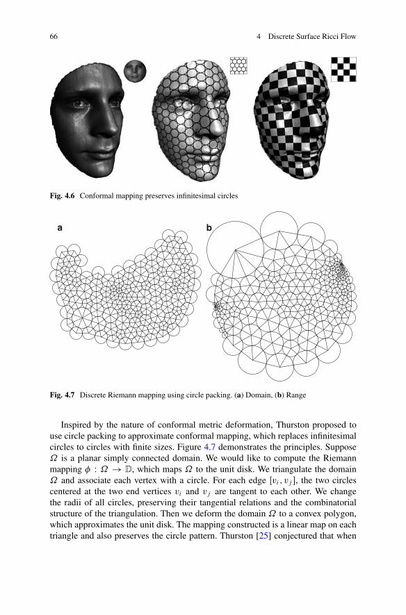
66 4 Discrete Surface Ricci Flow
Fig. 4.6 Conformal mapping preserves infinitesimal circles
a b
Fig. 4.7 Discrete Riemann mapping using circle packing. (a) Domain, (b) Range
Inspired by the nature of conformal metric deformation, Thurston proposed touse circle packing to approximate conformal mapping, which replaces infinitesimalcircles to circles with finite sizes. Figure 4.7 demonstrates the principles. Suppose˝ is a planar simply connected domain. We would like to compute the Riemannmapping � W ˝ ! D, which maps ˝ to the unit disk. We triangulate the domain˝ and associate each vertex with a circle. For each edge Œvi ; vj �, the two circlescentered at the two end vertices vi and vj are tangent to each other. We changethe radii of all circles, preserving their tangential relations and the combinatorialstructure of the triangulation. Then we deform the domain ˝ to a convex polygon,which approximates the unit disk. The mapping constructed is a linear map on eachtriangle and also preserves the circle pattern. Thurston [25] conjectured that when

4.2 Euclidean Discrete Surface Ricci Flow 67
γk
γj
γi vi
vj vk
φki
φij
φjk
ljklij
lki
Fig. 4.8 Circle packing metric
the tessellation goes to infinitely finer, then the piecewise linear map converges tothe real Riemann mapping. The conjecture was proved by Rodin and Sullivan [21].
Thurston’s idea can be applied for surfaces as well. Given a surface, we computea triangulation, then associate each vertex with a circle; the circles associated withthe end vertices of an edge Œvi ; vj � may intersect each other with a nonobtuse angle�ij , as shown in Fig. 4.8. In fact, each circle is a cone in R
3, the circle center is theapex, and the radius is the lateral height. For simplicity, we still call these conescircles. The difference between 2� and the cone angle is called discrete curvatureat the vertex. During the deformation, we only change the circle radii and keepthe combinatorial structure of the triangulation and the intersection angles �ij ’s.Then the discrete curvatures at the vertices (cone angles) will change accordingly.Intuitively, if we enlarge the radius at one vertex, then it becomes sharper and itscurvature increases; similarly, if we reduce the radius, then it becomes flatter and itscurvature decreases. Suppose we want to find a conformal mapping to “flatten” theface surface in Fig. 4.5 to the plane. Thurston’s algorithm is as follows: At each step,we sort the vertices according to the absolute values of their curvatures, pick the onewith the greatest absolute value. If its curvature is positive, then reduce its radius; ifits curvature is negative, then increase its radius, until its curvature becomes 0. Allthe other radii are kept unchanged during the process. Then we repeat the procedure,eventually, all the interior vertices have zero curvatures. Namely, the surface is flat.Each triangle on the surface is mapped to a planar triangle. The piecewise linearmap from the surface to the plane is an approximation of the Riemann mapping.If we subdivide the surface triangulation infinite times, then the discrete mappingsconverge to the real smooth Riemann mapping.
In the following, we discuss the discrete surface Ricci flow theory based onThurston’s circle packing. Thurston’s circle packing has been generalized to manydifferent configurations. The main theorems hold for all other variations as well.We will give a coherent framework to unify all the configurations in the laterdiscussion.

68 4 Discrete Surface Ricci Flow
4.2.2 Discrete Conformal Metric Deformation
Figure 4.8 illustrates Thurston’s circle packing metric. Let ˙ be a triangular mesh.We associate each vertex vi with a circle with radius �i . On one triangle faceŒvi ; vj ; vk�, the circle at vi and the circle at vj intersect at the angle �ij ; the lengthof the edge Œvi ; vj � is denoted as lij , which is given by
l2ij D �2i C �2j C 2�i�j cos�ij :
Definition 4.9 (Circle Packing Metric). A circle packing metric is a triple.˙;˚; � /, where ˙ represents the triangulation, ˚ the intersection angles and� the radii,
˚ D f�ij j8eij g; � D f�i j8vig:
In practice, it is more convenient to use the logarithm of the circle radius, whichis the discrete analogy to the concept of conformal factor in the smooth case.
Definition 4.10 (Discrete Conformal Factor). Discrete conformal factor on amesh ˙ is a function defined on each vertex u W V ! R,
ui D log �i :
In the smooth case, changing a Riemannian metric by a scalar function, g !e2ug, is called a conformal metric deformation. The discrete analogy to this is asfollows.
Definition 4.11 (Discrete Conformal Equivalence). Two circle packing metrics.˙k; ˚k; �k/, k D 1; 2, are conformally equivalent if ˙1 D ˙2 and ˚1 D ˚2.
We can also say that the circle packing metric .˙1; ˚1; �1/ is deformed to.˙2; ˚2; �2/ conformally. Namely, if we only change the circle radii and keepthe combinatorial structure and the intersection angles, then the discrete metricdeformation is conformal.
4.2.3 Euclidean Derivative Cosine Law
On a smooth surface, the Riemannian metric determines its Gauss curvature. Thisalso holds for discrete surfaces. The edge lengths determine the corner angles bycosine law. During the Ricci flow, the metric deforms smoothly, therefore we needto study the derivative cosine law.
Suppose Œvi ; vj ; vk� is a Euclidean triangle, as shown in Fig. 4.9. We treat eachcorner angle �i ; �j ; �k as the function of edge lengths li ; lj ; lk , respectively. Thenthe derivative of �i .li ; lj ; lk/ with respect to the edge lengths li ; lj ; lk are given bythe following lemma.

4.2 Euclidean Discrete Surface Ricci Flow 69
Fig. 4.9 A Euclideantriangle
Lemma 4.1 (Derivative Cosine Law).
@�i
@liD li
A;@�i
@ljD �@�i
@licos �k;
where A D lj lk sin �i is the double of the triangle area.
Proof. The proof is by direct computation. From the Euclidean cosine law,
2lj lk cos �i D l2j C l2k � l2i :
On both sides, taking the derivative with respect to li , we obtain @�i@li
D liA
; takingthe derivative with respect to lj , we get
@�i
@ljD � li cos �k
AD �@�i
@licos �k: ut
We rewrite the lemma in the matrix format,
0@ d�id�jd�k
1A D �1
A
0@ li 0 0
0 lj 0
0 0 lk
1A0@ �1 cos �k cos �j
cos �k �1 cos �icos �j cos �i �1
1A0@ dlid ljd lk
1A : (4.1)
Suppose the triangle is with a circle packing, then we define the power center asfollows.
Definition 4.12 (Power Center). Given a triangle Œvi ; vj ; vk�with a circle packing,the unique circle orthogonal to three circles at the vertices is called the power circle.The center of the power circle is called the power center.
As shown in Fig. 4.10, two intersecting circles have a common chord. Threecommon chords intersect at the power center o. Through the power center, we drawthree lines perpendicular to three edges, hi ; hj ; hk , intersecting with the edges at
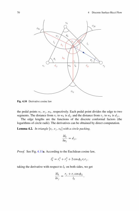
70 4 Discrete Surface Ricci Flow
vi vj
vk
li
lk
lj
θi
θk
θj
φjkφki
φij
o
hk
hi
djiwk
wj
wi
dij
hj
Fig. 4.10 Derivative cosine law
the pedal points wi ;wj ;wk , respectively. Each pedal point divides the edge to twosegments. The distance from vi to wk is dij and the distance from vj to wk is dji .
The edge lengths are the functions of the discrete conformal factors (thelogarithms of circle radii). The derivatives can be obtained by direct computation.
Lemma 4.2. In triangle Œvi ; vj ; vk� with a circle packing,
@lk
@ujD dji :
Proof. See Fig. 4.11a. According to the Euclidean cosine law,
l2k D r2i C r2j C 2 cos�ij ri rj ;
taking the derivative with respect to lk on both sides, we get
@lk
@rjD rj C ri cos�ij
lk;

4.2 Euclidean Discrete Surface Ricci Flow 71
vivj
vk
li
lk
lj
θi
θk
θj
φjkφki
φij
dji
τji
vi vj
vk
li
lk
lj
θi
θk
θj
φjkφki
φij
o
hk
hihj
a b
Fig. 4.11 Derivative relation between edge length (or corner angle) and conformal factor
therefore
@lk
@ujD rj
@lk
@rjD 2r2j C 2ri rj cos�ij
2lkD l2k C r2j � r2i
2lk
D 2lkrj cos �j i
2lkD rj cos �j i D dji :
utNamely,
0@ dlid ljd lk
1A D
0B@
12li
0 0
0 12lj
0
0 0 12lk
1CA0B@
0 l2i C r2j � r2k l2i C r2k � r2jl2j C r2i � r2k 0 l2j C r2k � r2il2k C r2i � r2j l2k C r2j � r2i 0
1CA0@ duidujduk
1A :
(4.2)
Furthermore, 0@ dlid ljd lk
1A D
0@ 0 djk dkjdik 0 dkidij dj i 0
1A0@ duidujduk
1A : (4.3)
Now we can show a property for dij .
Lemma 4.3. For the triangle Œvi ; vj ; vk� with a circle packing,
d2ij C d2jk C d2ki D d2j i C d2kj C d2ik:
Proof. By the Pythagorean theorem,
d2ij C h2k D d2ik C h2j ; d2jk C h2i D d2j i C h2k; d
2ki C h2j D d2kj C h2i :
Adding both sides, we complete the proof. ut

72 4 Discrete Surface Ricci Flow
vi vj
vk
li
lk
lj
θi
θk
θj
φjk
φki
φij
o
hk
hi
dji
djk
θj
di
Fig. 4.12@�i
@ujD hk
lk
The following symmetry lemma is crucial to the whole discrete Ricci flow theory.
Lemma 4.4 (Symmetry). In a triangle Œvi ; vj ; vk� with a circle packing,
@�i
@ujD @�j
@uiD hk
lk;@�j
@ukD @�k
@ujD hi
li;@�k
@uiD @�i
@ukD hj
lj; (4.4)
and
@�i
@uiD � @�i
@uj� @�i
@uk;@�j
@ujD �@�j
@uk� @�j
@ui;@�k
@ukD �@�k
@ui� @�k
@uj: (4.5)
Proof. See Fig. 4.11b. First we prove the equations in (4.4). From Lemma 4.1,
@�i
@ujD @�i
@li
@li
@ujC @�i
@lk
@lk
@ujD @�i
@li
�@li
@uj� @lk
@ujcos �j
�:
From Lemma 4.2, the right-hand side of the above equation equals
li
A.djk � dji cos �j / D di li
li lk sin �jD hk sin �jlk sin �j
D hk
lk;
where di D djk � dji cos �j , as shown in Fig. 4.12.Then we prove the equations in (4.5). Because �i C �j C �k D � ,

4.2 Euclidean Discrete Surface Ricci Flow 73
@�i
@uiD �@�j
@ui� @�k
@uiD � @�i
@uj� @�i
@uk:
utWe formulate the lemma in the matrix format by combining the matrix formu-
lae (4.1) and (4.3),
0@ d�id�jd�k
1A D �
0BB@
hklk
C hjlj
� hklk
� hjlj
� hklk
hklk
C hili
� hili
� hjlj
� hili
hjlj
C hili
1CCA0@ duidujduk
1A : (4.6)
Now let’s consider the admissible space of .ui ; uj ; uk/.
Lemma 4.5 (Admissible Space). For any three nonobtuse angles �ij ; �jk; �ki 2Œ0; �
2� and any three positive numbers ri ; rj ; rk , there is a configuration of three
circles in Euclidean geometry, unique up to isometry, having radii .ri ; rj ; rk/ andmeeting in angles .�ij ; �jk; �ki /.
Proof. It is sufficient and necessary to show that the triangle inequality holds.
maxfr2i ; r2j g < r2i C r2j C 2ri rj cos�ij � .ri C rj /2;
maxfri ; rj g < lk � ri C rj ;
so
lk � ri C rj < li C lj :
utTherefore, if the angles �ij ; �jk; �ki are nonobtuse, then the admissible space for
.ui ; uj ; uk/ is R3.
Lemma 4.6. The differential form
! D �idui C �j duj C �kduk
is an exact 1-form.
Proof. Because @�i@uj
D @�j@ui
,
d! D�@�i
@uj� @�j
@ui
�duj ^ dui C
�@�j
@uk� @�k
@uj
�duk ^ duj
C�@�k
@ui� @�i
@uk
�dui ^ duk D 0:
Therefore ! is a closed 1-form. Furthermore, the admissible space for .ui ; uj ; uk/ isR3, which is simply connected, so ! is exact. ut

74 4 Discrete Surface Ricci Flow
Because ! is an exact 1-form, it is the gradient of a function, which is the discreteRicci energy defined on all the circle packing metrics on the single triangle withintersection angles .�ij ; �jk; �ki /.
Definition 4.13 (Discrete Ricci Energy). The discrete Ricci energy is given by
E.ui ; uj ; uk/ DZ .ui ;uj ;uk/
.0;0;0/
!:
Theorem 4.2 (Concavity of Discrete Ricci Energy). The Ricci energyE.ui ; uj ; uk/is strictly concave on the subspace ui C uj C uk D 0.
Proof. From Lemma 4.6, the gradient rE D .�i ; �j ; �k/. From Lemma 4.4, theHessian matrix is
H D
0B@
@�i@ui
@�i@uj
@�i@uk
@�j@ui
@�j@uj
@�j@uk
@�k@ui
@�k@uj
@�k@uk
1CA D �
0BB@
hklk
C hjlj
� hklk
� hjlj
� hklk
hklk
C hili
� hili
� hjlj
� hili
hjlj
C hili
1CCA :
The negative of the Hessian matrix �H is diagonal dominant, with null space.1; 1; 1/. On the subspace uiCuj Cuk D 0,H is strictly negative definite. Thereforethe discrete Ricci energy E.ui ; uj ; uk/ is strictly concave. ut
4.2.4 Discrete Ricci Energy
Now we generalize the discrete Ricci energy to the whole triangular mesh.
Definition 4.14 (Edge Weight). Suppose Œvi ; vj � is an interior edge of a triangularmesh ˙ , adjacent to two faces Œvi ; vj ; vk� and Œvj ; vi ; vl �. Suppose the mesh is witha circle packing metric. Each face has a power center, ok for Œvi ; vj ; vk� and ol forŒvj ; vi ; vl �. The distances from ok; ol to Œvi ; vj � are hk and hl , respectively. Thelength of Œvi ; vj � is lk . After the two faces are flattened, the edge weight for Œvi ; vj �is given by
wij D jok � ol jjvi � vj j D hk C hl
lk:
If Œvi ; vj � is a boundary edge, draw a line from ok perpendicular to the edge, and thepedal point is wk , then the edge weight is given by
wij D jok � wkjjvi � vj j D hk
lk:

4.2 Euclidean Discrete Surface Ricci Flow 75
vi
vj
vkvl
ok ol
wk
θijk θi
jl
vi vj
vk
ok
wk
Fig. 4.13 Edge weight wij
Lemma 4.7. Suppose Œvi ; vj � is an edge on the mesh ˙ with a circle packingmetric. Then
@Ki
@ujD @Kj
@uiD �wij : (4.7)
Proof. See Fig. 4.13. Suppose Œvi ; vj � is an interior edge. According to (4.4),
@�jki
@ujD jok � wkj
jvi � vj j ;@�
jli
@ujD jol � wkj
jvi � vj j ;
we have
@Ki
@ujD �@�
jki
@uj� @�
jli
@ujD �jok � ol j
jvi � vj j D �wij :
Similarly, if Œvi ; vj � is a boundary edge, then
@Ki
@ujD �@�
jki
@ujD �jok � wkj
jvi � vj j D �wij :
Therefore, we get
@Ki
@ujD @Kj
@ui:
utLemma 4.8. Suppose vi is a vertex of a mesh˙ with a circle packing metric. Then
@Ki
@uiD �
Xj¤i
@Ki
@ujDXj¤i
wij : (4.8)

76 4 Discrete Surface Ricci Flow
Proof. Consider all the faces adjacent to vi , Œvi ; vj ; vk�, then according to (4.4)and (4.5),
@�jki
@uiD �@�
kij
@ui� @�
ij
k
@ui;
therefore
@Ki
@uiD �
Xjk
@�jki
@uiDXjk
@�kij
@uiC @�
ij
k
@ui
!D �
Xj
@Kj
@uiDXj
wij :
utDefinition 4.15 (Admissible Metric Space). Suppose ˙ is a triangular mesh. Fixthe circle intersection angles ˚ D f�ij g. Let the vector of logarithms of circleradii be u D .u1; u2; : : : ; un/T . Then if the triangle inequality holds on all faces of˙ , namely, .˙;˚; � / is a circle packing metric, then we say u is admissible. Thespace of all admissible u vectors is called the admissible metric space for .˙;˚/,denoted as U.˙;˚/.
Definition 4.16 (Curvature Map). Given an admissible metric u 2 U.˙;˚/, itinduces the Gauss curvature on the mesh. The Gauss curvatures on all vertices arerepresented as a vector k D .K1;K2; : : : ; Kn/ 2 R
n. The mapping from metric u tothe curvature vector k is called the curvature map, denoted as � W U.˙;˚/ ! R
n.
The image of the curvature map is called the admissible curvature space.
Definition 4.17 (Admissible Curvature Space). Suppose ˙ is a triangular mesh.Fix the circle intersection angles ˚ D f�ij g. Then the space of all possible Gausscurvatures k D .K1;K2; : : : ; Kn/, which is induced by an admissible metric u 2U.˙;˚/, is called the admissible curvature space, denoted as K.˙;˚/,
K.˙; �/ WD �.U.˙;˚//:
Due to the discrete Gauss–Bonnet Theorem 4.1, the total curvature is determinedby the topology of ˙ . Therefore
K.˙; �/ �(
nXiD1
Ki D 2�.˙/
):
Lemma 4.9 (Admissible Metric Space). Given a triangular mesh ˙ , fix circleintersection angles ˚ , such that all �ij ’s are nonobtuse angles, �ij 2 Œ0; �
2�, then
the admissible metric space for .˙;˚/ is Rn,
U.˙;˚/ D Rn:

4.2 Euclidean Discrete Surface Ricci Flow 77
Proof. According to Lemma 4.5, for each face Œvi ; vj ; vk�, the admissible metricspace U.Œvi ; vj ; vk�; Œ�ij ; �jk; �ki �/ is Rn. The admissible metric space of the wholemesh ˙ is the intersection of the admissible metric spaces of all faces,
U.˙;˚/ D\
Œvi ;vj ;vk �2˙U.Œvi ; vj ; vk�; Œ�ij ; �jk; �ki �/ D R
n:
utCorollary 4.1. The differential form
! DnXiD1
Kidui
is an exact 1-form.
Proof. Lemma 4.7 shows ! is closed. Because the admissible metric space is simplyconnected, ! is exact. ut
So we can define the Ricci energy, using ! as the gradient.
Definition 4.18 (Discrete Ricci Energy). The discrete Ricci energy is defined onthe admissible metric space for .˙;˚/,
E.u1; u2; : : : ; un/ DZ .u1;u2;:::;un/
.0;0;:::;0/
!:
Theorem 4.3 (Convexity of Ricci Energy). The discrete Ricci energy is strictlyconvex on the space,
nXiD1
ui D 0:
Proof. Here we give two proofs. The first proof is based on the concavity of thediscrete Ricci energy on each triangle. Suppose there are V0 interior vertices andV1 boundary vertices. Let E.˙/ represent the Ricci energy of the whole mesh andE.Œvi ; vj ; vk�/ the energy on the face. Then
E.˙/ DXvi 62@˙
2�ui CXvj2@˙
�uj �X
Œvi ;vj ;vk �2˙E.Œvi ; vj ; vk�/:
The linear terms won’t affect the convexity. For all the faces, according to Theo-rem 4.2, E.Œvi ; vj ; vk�/ is strictly concave on the space ui C uj C uk D 0. Thenull space of the Hessian of E.Œvi ; vj ; vk�/ is ui D uj D uk . Therefore, the nullspace of the Hessian of E.˙/ is the intersection of all the face null spaces, namely,the one dimensional space spanned by .1; 1; 1; : : : ; 1/T . In the complement spaceP
i ui D 0, E.˙/ is the negative sum of concave functions E.Œvi ; vj ; vk�/, so it isstrictly convex.

78 4 Discrete Surface Ricci Flow
The second proof is to directly compute the Hessian matrix of the energy. Thegradient of E.˙/ is
rE.˙/ D .K1;K2; : : : ; Kn/T :
Therefore, the element of the Hessian matrix
@2E.˙/
@ui @ujD @Ki
@uj:
According to Lemmas 4.7 and 4.8, if vi is adjacent to vj , then @Ki@uj
D �wij ,
otherwise @Ki@uj
D 0. The diagonal elements @Ki@ui
D Pj¤i wij . Therefore, the
Hessian matrix is diagonal dominant, with one dimensional null space, spanned by.1; 1; : : : ; 1/T . In the space
Pi ui D 0, the energy is strictly convex. ut
Note that the differential of the curvatures and the logarithm of radius satisfy theLaplace equation
dKi DXj
wij .dui � duj /:
The admissible curvature space is also convex, which can be described by thefollowing lemma.
Lemma 4.10 (Admissible Curvature Space). Suppose .˙;˚/ is a triangularmesh with a circle packing, and all the circle intersection angles are nonobtuse,8�ij 2 ˚ , �ij 2 Œ0; �
2�. Let I be a proper subset of vertices V . FI is the collection
of faces, whose vertices are in I . The link of I , denoted as Lk.I /, is the set of pairs.e; v/, where e is an edge whose vertices are not in I , and vertex v 2 I , so that.e; v/ form a triangle. Then for any admissible curvature, the following inequalityholds,
Xvi2I
Ki > �X
.e;v/2Lk.I /.� � �.e//C 2�.FI /: (4.9)
Given a curvature vector k D .K1;K2; : : : ; Kn/, if for any proper subset I theinequality (4.18) holds, then the curvature is admissible.
The details of the proof can be found in [6].
4.2.5 Global Rigidity
In the smooth case, the Gauss curvature is determined by the Riemannian metric.The inverse is not true. Different Riemannian metrics may induce the same Gauss

4.2 Euclidean Discrete Surface Ricci Flow 79
x1
x2
f(x)
Ω
∇f (x)
x → ∇f (x)
Fig. 4.14 Legendretransformation
curvature function, but if the Riemannian metrics are restricted within a conformalclass, then the Gauss curvature can essentially determine the metric. Namely, thesolution to the Yamabe problem,
� NK D e�2�.K ��g�/Nkg D e��.kg � @n;g�/;
is essentially unique. In the discrete case, the discrete metrics determine the discretecurvatures. Inversely, the discrete curvatures determine the discrete conformalRiemannian metrics. This uniqueness is called the rigidity. In the following, therigidity will be proved based on the Legendre transformation.
Legendre Transformation
Suppose ˝ � Rn is a convex domain. A C2 function f W ˝ ! R is a convex
function, such that its Hessian matrix
�@2f
@xi@xj
�> 0
is positive definite.
Definition 4.19 (Legendre Transformation). The gradient map
� W x ! rf .x/ D�@f
@x1;@f
@x2; : : : ;
@f
@xn
�T
is called a Legendre transformation. See Fig. 4.14.

80 4 Discrete Surface Ricci Flow
Theorem 4.4. Suppose ˝ � Rn is a convex domain. A C2 function f W ˝ ! R
is a convex function. Then the Legendre transformation � W ˝ ! �.˝/ is a globaldiffeomorphism.
Proof. The Jacobian matrix of � is the Hessian of f , which is positive definite andinvertible. Therefore � is a local diffeomorphism, namely, for each point p 2 ˝,there exists a neighborhood of p, such that the restriction of � on the neighborhoodis a diffeomorphism. But globally, the mapping may not be one-to-one.
Now we need to show � W ˝ ! �.˝/ is a global diffeomorphism. It is necessaryand sufficient to prove the injectivity.
Assume the map is not injective, there exist p1;p2 � ˝, p1 ¤ p2, such thatrf .p1/ D rf .p2/. Because˝ is convex, the line segment .1�t /p1Ctp2; t 2 Œ0; 1�is contained in ˝. The function g.t/ D f ..1 � t /p1 C tp2/ is convex, because
d2g.t/
dt2D .p2 � p1/TH.p2 � p1/ > 0;
where H is the Hessian matrix of f . Therefore dg.t/
dtis monotonous, but
g0.0/ D hrf .p1/;p2 � p1i D hrf .p2/;p2 � p1i D g0.1/
is a contradiction. Therefore, the mapping is injective and is a global diffeomor-phism. This completes the proof. ut
Now we come to the global rigidity for discrete Ricci flow.
Theorem 4.5 (Global Rigidity). Suppose ˙ is a triangular mesh, with circlepacking metrics .˙;˚; � /, where all the circle intersection angles ˚ are fixed andare nonobtuse. Then the curvature map
� W U.˙;˚/\�X
i
ui D 0
! K.˙;˚/
is a global diffeomorphism.
Proof. Consider the discrete Ricci energy E W U.˙;˚/ ! R, which is withC2 continuity. By Lemma 4.9, the domain U.˙;˚/ is convex, so is the inter-section between U.˙;˚/ and the hyperplane
Pi ui D 0. By Theorem 4.3,
on U.˙;˚/TfPi ui D 0g the energy is convex. The Legendre transformation
induced by the energy is the curvature map
� W .u1; u2; : : : ; un/ ! rE D .K1;K2; : : : ; Kn/:
By the discrete Gauss–Bonnet Theorem 4.1, the total curvatureP
i Ki D 2�.˙/.By Theorem 4.4, the curvature map is a global diffeomorphism. ut

4.2 Euclidean Discrete Surface Ricci Flow 81
4.2.6 Convergence Analysis
The discrete surface Ricci flow is given by
dri
dtD �Kiri ;
or equivalently, ui D log ri ,
duidt
D �Ki :
In practice, it is useful to consider the normalized Ricci flow.
Definition 4.20 (Normalized Discrete Surface Ricci Flow).
duidt
D NK �Ki ; (4.10)
where NK is the average vertex curvature, NK D 2�.˙/=n, and n is the number ofvertices.
It is easy to see that the normalized Ricci flow (4.10) is the negative gradient flowof the energy,
E.u/ DZ nX
iD1.Ki � NK/dui D
Z nXiD1
Kidui � NKnXiD1
ui :
If we ignore the linear term, then the energy is convex. It has a unique globalminimum, where the gradient is zero, namely, rE.u/ D .K1� NK;K2� NK; : : : ; Kn�NK/ is a zero vector. If the average curvature is in the admissible curvature space,
then the negative gradient flow leads to the global minimum. Therefore, we show theconvergence theorem. In order to check whether the average curvature is admissible,we can verify the inequality (4.18) for all proper vertex subsets.
Theorem 4.6 (Convergence of Discrete Ricci Flow). Suppose ˙ is a triangularmesh with nonobtuse intersection angles �ij 2 Œ0; �
2�. If for any proper subset of the
vertices I � V ,
2�jI j.˙/n
> �X
.e;v/2Lk.I /.� � �.e//C 2�.FI /;
then the discrete surface Ricci flow converges to the metric of constant curvature2�.˙/=n.
Furthermore, we can estimate the convergence rate of the discrete Ricci flow.

82 4 Discrete Surface Ricci Flow
Theorem 4.7 (Exponential Convergence Rate). The discrete surface Ricci flowconverges exponentially fast to the constant curvature metric, for every vertex vi ,
.Ki .t/ � NK/2 � c2e�c1t ;
where c1; c2 are positive constants.
In order to prove the convergence and convergence rate of the discrete Ricci flow,we need the following lemma.
Lemma 4.11. Suppose ˙ is a connected triangular mesh. Then there exists aconstant c3 > 0 depending only on ˙ , so that
nXiD1.Ki � NK/2 � c3
XŒvi ;vj �2˙
.Ki �Kj /2; (4.11)
for all time t > 0.
Proof. According to the Cauchy’s inequality hx; yi2 � hx; xihy; yi, let
x D .ai � a1; ai � a2; : : : ; ai � an/T ; y D .1; 1; : : : ; 1/;
then
.ai � Na/2 � 1
n
0@ nXjD1
.ai � aj /21A ;
where Na DPniD1 ain
. We obtain
nXiD1.Ki � NK/2 � 1
n
nXi;jD1
.Ki �Kj /2: (4.12)
On the other hand, since the surface˙ is connected, for any two vertices vi ; vj 2 ˙ ,there exists a shortest path between them. The path is represented as a sequence ofvertices vm1 D vi ; : : : ; vml D vj , so that vmk and vmkC1
are adjacent. The value
.Ki �Kj /2 D
l�1XkD1.Kmk �KmkC1
/
!2�
l�1XkD1.Kmk �KmkC1
/2:
Therefore
nXi;jD1
.Ki �Kj /2 � c3n
XŒvi ;vj �2˙
.Ki �Kj /2: (4.13)

4.2 Euclidean Discrete Surface Ricci Flow 83
By combining (4.12) and (4.13), we obtain
nXiD1.Ki � NK/2 � c3
XŒvi ;vj �2˙
.Ki �Kj /2:
This completes the proof for the lemma. utNow we prove the convergence theorems for the discrete Ricci flow.
Proof. During the flow, the energy E.u/ decreases monotonously. The path u.t/in the admissible metric space is contained in a compact subset, fujE.u/ � E0g,where E0 is the initial energy value. So all ui .t /’s are bounded. The edge weightswij ’s are smooth functions of u, therefore there exists a constant c4 > 0, such thatfor all Œvi ; vj � 2 ˙ ,
wij .t/ > c4; t 2 Œ0;1/: (4.14)
Consider the energy
g.t/ WDnXiD1.Ki .t/ � NK/2:
From n NK D PniD1 Ki .t/,
g.t/ DnXiD1.K2
i C NK2�2KiNK/D
nXiD1
K2i Cn NK2�
2
nXiD1
Ki
!NK D
nXiD1
K2i .t/�n NK2:
From K 0i D Pj wij .u0i � u0j / D P
j wij .Kj �Ki/,
g0.t/ WD 2
nXiD1
XŒvi ;vj �2˙
wijKi .Kj �Ki/:
By switching the order of i; j , we also have
g0.t/ D 2
nXjD1
XŒvi ;vj �2˙
wijKj .Ki �Kj /:
Thus from (4.14) and (4.11),
g0.t/ D�X
Œvi ;vj �2˙wij .Ki �Kj /
2 � �c4X
Œvi ;vj �2˙.Ki �Kj /
2 � �c4c3
nXiD1.Ki � NK/2
D �c4c3g.t/:

84 4 Discrete Surface Ricci Flow
This implies that g.t/ � c2e� c4c3 t for all time t 0 and for some constant c2. Then
we obtain
.Ki .t/ � NK/2 �nXiD1.Ki � NK/2 D g.t/ � c2e
� c4c3 t :
Let c1 be c4c3
. This completes the proof. ut
4.2.7 Unified Euclidean Discrete Surface Ricci Flow
Thurston’s circle packing has been generalized to different schemes. This greatlyincreases the flexibility for practical purposes. All the schemes share the samegeometric principles. Therefore, a unified theory can be established to cover all theschemes.
Generalized Schemes
Figure 4.15 illustrates the general schemes, where the power circles are in red color.Frame (a) shows the classical Thurston’s circle packing, where the edge length andthe circle radii satisfy the relation
l2k D �2i C �2j C 2�i�j cos�k:
where �k is the intersection angle between circles at vi and vj . Algebraically, thisformula is generalized to the following form
l2k D ˛i�2i C ˛j �
2j C 2�i�j �k; (4.15)
where
˛i ; ˛j 2 fC1; 0;�1g; �k 0:
Frame (b) shows the tangential circle packing, where the circle intersection anglesbecome zeros, namely, all circles are tangential to each other, �k D 0. Frame (c)shows the inversive distance circle packing, where all the circles are disjoint, thecosine of �k is replaced by the �k , the so-called inversive distance, which is greaterthan 1. Frame (d) shows the discrete Yamabe flow scheme, where all ˛i ’s are 0’s.Frame (e) is the imaginary radius circle packing, namely, all radii are imaginarynumbers, and ˛i ’s equal �1.

4.2 Euclidean Discrete Surface Ricci Flow 85
a b c
o
djidij
dik
dki dkj
djk
vjvi
vk
hk
hi
hj
lk
lilj
θi θj
θkwj wi
wk
d e f
Fig. 4.15 Generalized schemes (a) Thurston’s circle packing: l2k D �2i C �2j C 2�i �j cos�k ,(b) Tangential circle packing: lk D �i C �j , (c) Inversive distance circle packing: l2k D �2i C�2j C 2�i �j �k , (d) Discrete Yamabe flow: l2k D 2�i �j �k , (e) Imaginary radius circle packing:l2k D ��2i � �2j C 2�i �j �k , (f) Common configuration
We define the generalized power circle and the power center. For the schemeson the top row, a–c the power circle is a circle orthogonal to three circlescentered at the vertices, and its center is the power center. For the discrete Yamabeflow scheme d, the power circle is the circumcircle and the power center is thecircumcenter. The power circle for the imaginary radius circle packing e is morecomplicated. Suppose the circle radii at vi ; vj ; vk are �i ; �j ; �k , respectively. Wetranslate vi ; vj ; vk vertically (perpendicularly to the plane containing the triangle) topi ; pj ; pk , respectively, such that the vertical distances between the correspondingpairs are �2i ; �
2j and �2k , respectively. We draw a hemisphere S through pi ; pj , and
pk , and its equator is on the same plane containing the triangle. The equator of S isthe power circle, and the spherical center is the power center. Algebraically, all thepower centers satisfies the following equidistance condition,
jvi � oj2 � ˛i�2i D jvj � oj2 � ˛j �2j D jvk � oj2 � ˛k�2k ;
where o is the power center.All the schemes share the same configuration as illustrated in frame f. We draw
perpendicular lines from the power center to each edge. The distances from thepower center to each edge are hi ; hj , and hk , respectively. The pedal points divideeach edge into two segments. Suppose the pedal point on Œvi ; vj � is wk , the length

86 4 Discrete Surface Ricci Flow
of Œvi ;wk� is dij , and the length of Œvj ;wk� is dji . We can show all the key formulaefor Thurston’s circle packing hold for the generalized schemes. From the followingequations,
d2ij C h2k D d2ik C h2j D jvi � oj2;d 2jk C h2i D d2j i C h2k D jvj � oj2;d 2ki C h2j D d2kj C h2i D jvk � oj2;
we obtain the relation
d2ij C d2jk C d2ki D d2j i C d2ik C d2kj :
The differential relation between edge lengths and the conformal factors also holds,
@lk@ui
D dij ;@lk@uj
D dji ;@li@uj
D djk;@li@uk
D dkj ;@lj@ui
D dik;@lj@uk
D dki :
Unified Theorems
All the schemes can be unified as the discrete conformal structure [9].
Definition 4.21 (Discrete Conformal Structure). A triangular mesh ˙ admits adiscrete conformal structure if it admits a length function l W E ! R, such that
1. lij .ui ; uj / is symmetric in ui and uj , where u W V ! R is an arbitrary functiondefined on V .
2. lij D dij C dji , where
@lij
@uiD dij :
3. For any triangle Œvi ; vj ; vk�,
d2ij C d2jk C d2ki D d2j i C d2kj C d2ik:
The concept of discrete conformal structure is more general, different schemescan be combined together, as shown in Fig. 4.16, where the inversive distance circlepacking (at vi ), discrete Yamabe flow (at vk), and imaginary radius circle packing(vj ) schemes are mixed together. The edge lengths are given by
l2k D �2i � �2j C 2�i�j �k; l2j D �2i C 2�i�k�j ; l
2i D ��2j C 2�j �k�i :

4.2 Euclidean Discrete Surface Ricci Flow 87
vi vj
vk
lk
li
lj
o
dij dji
djk
dkj
dik
dki
hj
hi
hk
Fig. 4.16 Mixed scheme
With a general discrete conformal structure, the following theoretical resultshold. The differential relations between the inner angles and the conformal factorsare given by
@�i
@ujD @�j
@uiD hk
lk;@�j
@ukD @�k
@ujD hi
li;@�k
@uiD @�i
@ukD hj
lj:
Also, the following formulae hold for all the schemes,
@�i
@uiD � @�i
@uj� @�i
@uk;@�j
@ujD �@�j
@uk� @�j
@ui;@�k
@ukD �@�k
@ui� @�k
@uj:
These equations imply the following lemma.
Lemma 4.12. Given a triangle Œvi ; vj ; vk� with a discrete conformal structure,assume three discrete conformal factors are ui ; uj ; uk , and the three inner anglesare �k; �i ; �j . The 1-form
! D �idui C �j duj C �kduk
is a closed 1-form.
Then we can define discrete Ricci energy on one triangle.
Definition 4.22 (Discrete Ricci Energy). Given a triangle Œvi ; vj ; vk� with a dis-crete conformal structure, assume three discrete conformal factors are ui ; uj ; uk ,and the three inner angles are �k; �i ; �j . The discrete Ricci energy is defined as
E.ui ; uj ; uk/ DZ .ui ;uj ;uk/
.0;0;0/
!:
The following theorem holds for a triangle with a discrete conformal structure.

88 4 Discrete Surface Ricci Flow
Theorem 4.8. Given a triangle Œvi ; vj ; vk� with a discrete conformal structure,assume three discrete conformal factors are ui ; uj ; uk . The discrete Ricci energyis convex on the plane ui C uj C uk D 0.
We can define the discrete conformal structure for a triangular mesh˙ and definethe discrete Ricci energy on the whole mesh. Then we can show the convexity ofthe Ricci energy, but we cannot show the convexity of the admissible metric space.Therefore, we can get local rigidity result, not global rigidity (see Theorem 4.5for the global rigidity of the Thurston’s circle packing). Namely, the mappingfrom a discrete conformal metric to the discrete Gauss curvature is locally one-to-one. Furthermore, for general schemes, there is no explicit method to describethe admissible curvature space (see Lemma 4.10 for the admissible curvature spaceof the Thurton’s circle packing).
Geometric Interpretation of Ricci Energy
The discrete Ricci energy on a triangle with a conformal structure has geometricinterpretation, which is the volume of a hyperbolic tetrahedron. The upper half spacemodel of three-dimensional hyperbolic space H
3 is the space
H3 D f.x; y; z/ 2 R
3jz > 0g
with the Riemannian metric
dx2 C dy2 C d z2
z2:
The xy-plane is the plane at infinity. Geodesics are circular arcs perpendicularto the xy-plane. Hyperbolic planes are hemispheres, whose equators are on thexy-plane. An ideal tetrahedron has four vertices at infinity, namely, on xy-plane.If some vertices exceed the xy-plane, then the tetrahedron is called a truncatedideal tetrahedron. Basically, a triangle with a conformal structure corresponds to atruncated ideal hyperbolic tetrahedron in H
3, and the discrete Ricci energy equalsthe volume of the hyperbolic tetrahedron up to a constant. In the following, wevisualize the Ricci energy for different schemes.
The geometric meanings of discrete Ricci energy for Thurston’s circle packing,tangential circle packing, and inversive distance circle packing are illustrated inFigs. 4.17, 4.18, and 4.19, respectively. The truncated hyperbolic ideal tetrahedraare constructed as follows. First, we construct a prism in H
3, which is the directproduct of the triangle Œvi ; vj ; vk� with the vertical line segment Œ0; c�, where c > 0is sufficiently large. Through each vertex circle and the power circle, we construct ahemisphere. Each hemisphere is a hyperbolic plane. We cut off the prism by thesefour hyperbolic planes to obtain the truncated idea tetrahedron.

4.2 Euclidean Discrete Surface Ricci Flow 89
vi vj
vk
CiCj
Ck
C0odij dji
lij
hk
wk
wiwjdjk
dkj
dik
dki
hi
hj
Fig. 4.17 Thurston’s circle packing scheme
vi vj
vk
wk
wiwj
dij dji
djk
dkjdki
dik
o
hk
hi
hjri rj
rk
CiCj
Ck
C0
Fig. 4.18 Tangential circle packing scheme
vi vj
vk
CiCj
Ck
C0
o
dij dji
lij
hk
wk
wiwj
djk
dkj
dik
dki
hi
hj
θjθi
θk
τij τij
τjk
τjk
τik
τik
Fig. 4.19 Inversive distance circle packing scheme
Figure 4.20 visualizes the Ricci energy for discrete Yamabe flow scheme. Theprism is cut off by the hyperbolic plane through the power circle. Then for eachvertex vi , we construct a sphere tangent to vi with (Euclidean) radius ri . Then thetetrahedron is cut off by the spheres. The volume of the resulting tetrahedron is thediscrete Ricci energy up to a constant.
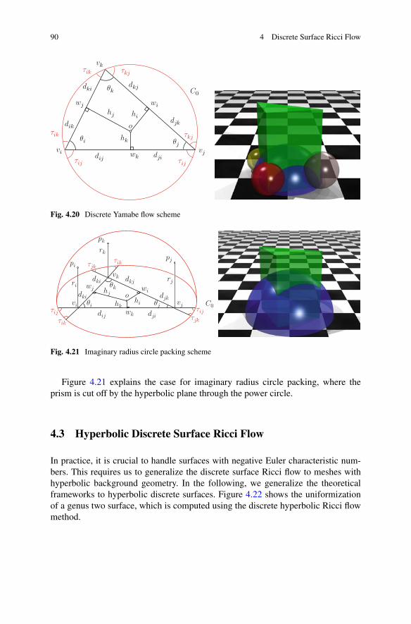
90 4 Discrete Surface Ricci Flow
vi vj
vk
C0
o
dij dji
dkj
djk
dki
dik
wk
wiwj
hk
hj hi
τkj
τkj
τijτij
τik
τik
θk
θi θj
Fig. 4.20 Discrete Yamabe flow scheme
vi vj
vk
oC0
rirj
rk
wk
wiwj
dij dji
djk
dkjdki
dkihj
hihkτij τij
τjk
τjkτik
τik
θi θj
θk
pi
pk
pj
Fig. 4.21 Imaginary radius circle packing scheme
Figure 4.21 explains the case for imaginary radius circle packing, where theprism is cut off by the hyperbolic plane through the power circle.
4.3 Hyperbolic Discrete Surface Ricci Flow
In practice, it is crucial to handle surfaces with negative Euler characteristic num-bers. This requires us to generalize the discrete surface Ricci flow to meshes withhyperbolic background geometry. In the following, we generalize the theoreticalframeworks to hyperbolic discrete surfaces. Figure 4.22 shows the uniformizationof a genus two surface, which is computed using the discrete hyperbolic Ricci flowmethod.

4.3 Hyperbolic Discrete Surface Ricci Flow 91
Fig. 4.22 Uniformization of a high genus surface using hyperbolic Ricci flow
4.3.1 Hyperbolic Derivative Cosine Law
The hyperbolic cosine law and sine law are given by
cos �i D cosh lj cosh lk � cosh lisinh lj sinh lk
;
sin �isinh li
D sin �jsinh lj
D sin �ksinh lk
:
The double area of the hyperbolic triangle is
A D sinh lj sinh lk sin �i :
Figure 4.23 shows a hyperbolic triangle and the hyperbolic circle packing.
Lemma 4.13 (Hyperbolic Derivative Cosine Law).
@�i
@liD sinh li
A;@�i
@ljD � sinh li
Acos �k:
Proof. From the hyperbolic cosine law,
cos �i D cosh lj cosh lk � cosh lisinh lj sinh lk
:
Taking derivative on both sides with respect to li , we get
� sin �i@�i
@liD � sinh li
sinh lj sinh lk;

92 4 Discrete Surface Ricci Flow
vi vj
vk
li
lk
lj
θi
θk
θj
vi vj
vk
lilj
lk
θi θj
θk φjk
φki
φij
Fig. 4.23 A hyperbolic triangle and hyperbolic circle packing
therefore
@�i
@liD sinh li
A:
Similarly,
cos �i D cosh lj cosh lk � cosh lisinh lj sinh lk
@�i
@ljD sinh lj cosh lk.sinh lj sinh lk/�.� cosh li C cosh lj cosh lk/ sinh lk cosh lj
� sin �i .sinh lj sinh lk/2
D .sinh l2j � cosh l2j / cosh lk sinh lk C cosh li cosh lj sinh lk
� sin �i sinh l2j sinh l2k
D � cosh lk C cosh li cosh lj�A sinh lj
D sinh li sinh lj cos �k�A sinh lj
D � sinh liA
cos �k:
utWe write the result in the matrix format,
0@ d�id�jd�k
1A D �1
A
0@ sinhi 0 0
0 sinhj 0
0 0 sinhk
1A0@ �1 cos �k cos �j
cos �k �1 cos �icos �j cos �i �1
1A0@ dlid ljd lk
1A : (4.16)

4.3 Hyperbolic Discrete Surface Ricci Flow 93
4.3.2 Thurston’s Circle Packing
Similarly to the Euclidean case, we can use Thurston’s circle packing for discreteconformal metric deformation. Then the relation between the edge length and thecircle radii is governed by the hyperbolic cosine law,
cosh li D cosh rj cosh rk C sinh rj sinh rkIjk;
where li is the length of the edge Œvi ; vj �, and Ijk is the cosine of the intersectionangle between two circles centered at vj and vk .
Lemma 4.14. The differential relation between the edge lengths and the circleradii is
dli D � cosh rk C cosh li cosh rjsinh li sinh rj
drj C � cosh rj C cosh li cosh rksinh li sinh rk
drk:
Proof.
cosh li D cosh rj cosh rk C sinh rj sinh rkIjk;
sinh lid li
drjD sinh rj cosh rk C cosh rj sinh rkIjk;
d li
drjD sinh rj cosh rk C cosh rj sinh rkIjk
sinh li:
Because
Ijk D cosh li � cosh rj cosh rksinh rj sinh rk
:
d li
drjD
sinh rj cosh rk C cosh rj sinh rkcosh li�cosh rj cosh rk
sinh rj sinh rk
sinh li
D sinh2 rj cosh rk C cosh rj cosh li � cosh2 rj cosh rksinh li sinh rj
D .sinh2 rj � cosh2 rj / cosh rk C cosh rj cosh lisinh li sinh rj
D cosh rj cosh li � cosh rksinh li sinh rj
:
ut

94 4 Discrete Surface Ricci Flow
We write the equation in matrix format,
0@ dlid ljd lk
1A D
0B@
1sinh li
0 0
0 1sinh lj
0
0 0 1sinh lk
1CAM
0B@
1sinh ri
0 0
0 1sinh rj
0
0 0 1sinh rk
1CA0@ dridrjdrk
1A ; (4.17)
where
M D
0B@
0 � cosh rkC cosh li cosh rj � cosh rjC cosh li cosh rk� cosh rkC cosh lj cosh ri 0 � cosh riC cosh lj cosh rk� cosh rjC cosh lk cosh ri � cosh riC cosh lk cosh rj 0
1CA:
Let the discrete conformal factor ui D log tanh ri2
, .a; b; c/ D .cosh li ; cosh lj ;cosh lk/, and .x; y; z/ D .cosh ri ; cosh rj ; cosh rk/. By the hyperbolic cosine law,we get the following lemma.
Lemma 4.15. The differential relations between the inner angles and discreteconformal factors are
0@ d�id�jd�k
1A D N
0@ duidujduk
1A ;
where
N D0@ 1 � a2 ab � c ca � bab � c 1 � b2 bc � aca � b bc � a 1 � c2
1A0B@
1a2�1 0 0
0 1b2�1 0
0 0 1c2�1
1CA0@ 0 ay � z az � ybx � z 0 bz � xcx � y cy � x 0
1A :
Proof. From ui D log tanh ri2
, we obtain dri D sinh ridui . Combining it with (4.16)and (4.17), we get the formula. utLemma 4.16. The differential form ! D �idui C �j duj C �kduk is closed.
Proof. By direct computation, for example,
@�i
@ujD @�j
@uiD z � ac � b
c2 � 1 x � bc � ac2 � 1 y:
utLemma 4.17. The admissible metric space is R3.
Proof. Because li � rj C rk � lj C lk , the triangle inequality holds for all possiblefri ; rj ; rkg. ut
Because the admissible metric space is simply connected, the closed 1-form isexact. We can define the discrete Ricci energy as
R!.

4.3 Hyperbolic Discrete Surface Ricci Flow 95
Lemma 4.18. The discrete Ricci energy
E.ui ; uj ; uk/ DZ .ui ;uj ;uk/
.0;0;0/
!
is strictly concave.
Proof. It is sufficient to show the Hessian matrix@�i@uj
�is negative definite. Suppose
we increase ui . Then the hyperbolic triangle area increases as well. According to theGauss–Bonnet theorem,
� � .�i C �j C �k/ D A;
therefore �i C �j C �k decreases,
@.�i C �j C �k/
@ui< 0:
This means
@�i
@ui< �@�j
@ui� @�k
@uiD � @�i
@uj� @�i
@uk:
On the other hand, @�i@uj
is positive. So the negative of the Hessian matrix is diagonaldominant, and the Hessian matrix is negative definite. The energy is strictly concave.
ut
4.3.3 Discrete Hyperbolic Ricci Energy
Let ˙ be a triangular mesh with hyperbolic background geometry, and ˚ be theangle intersection angles, such that for any edge Œvi ; vj �, �ij 2 Œ0; �
2�, and ui D
log tanh ri2
. We can directly show that
! DnXiD1
Kidui
is a closed 1-form. The admissible metric space for all circle-packing metricsu D .u1; u2; : : : ; un/ of .˙;˚/ is R
n. The discrete Ricci energyR! is strictly
convex. The curvature map � W .u1; u2; : : : ; un/ ! .K1;K2; : : : ; Kn/ is a globaldiffeomorphism.
Let I be a proper subset of vertices V . FI is the collection of faces, whosevertices are in I . The link of I , Lk.I / is the set of pairs .e; v/, where e is an edge

96 4 Discrete Surface Ricci Flow
whose vertices are not in I , and vertex v 2 I , so that .e; v/ forms a triangle. Givena curvature vector .K1;K2; : : : ; Kn/, if for any proper subset I � V , the followinginequality (4.18) holds,
Xvi2I
Ki > �X
.e;v/2Lk.I /.� � �.e//C 2�.FI /; (4.18)
then the curvature is admissible.
4.3.4 Generalized Schemes
Similarly to Euclidean case, Thurston’s circle packing can be generalized to differ-ent schemes for discrete hyperbolic Ricci flow. In the following, we only discusshyperbolic Yamabe flow; other schemes can be carried out similarly. HyperbolicYamabe flow is defined as
sinhyk
2D eui sinh
lk
2euj ;
where yk.t/ is the edge length during the flow, lk is the initial edge length, andyk.0/ D lk . Taking the derivative with respect to ui on both sides,
1
2cosh
yk
2
@yk
@uiD eui sinh
lk
2euj D sinh
yk
2;
we get
@yk
@uiD 2 tanh
yk
2D 2
sinh yk2
cosh yk2
D 2 sinh yk2
cosh yk2
cosh2 yk2
:
Since sinh 2x D 2 sinh x cosh x and cosh 2x D 2 cosh2 x � 1, we obtain
@yk
@uiD 2 sinh yk
coshyk C 1:
Therefore
0@dy1dy2dy3
1A D 2
0B@
sinh y1cosh y1C1 0 0
0sinh y2
cosh y2C1 0
0 0sinh y3
cosh y3C1
1CA0@0 1 11 0 1
1 1 0
1A0@du1du2du3
1A :
We use Ci ; Sj to represent cosh yi and sinhyj , respectively, and obtain

4.3 Hyperbolic Discrete Surface Ricci Flow 97
0@d�1d�2
d�3
1A D � 2
A
0@S1 0 0
0 S2 0
0 0 S3
1A0@ �1 cos �3 cos �2
cos �3 �1 cos �1cos �2 cos �1 �1
1A0B@
0 S1C1C1
S1C1C1
S2C2C1
0 S2C2C1
S3C3C1
S3C3C1
0
1CA0@du1du2du3
1A
D � 2
A
0BB@
S1S2 cos �3C2C1
C S1S3 cos �2C3C1
�S21C1C1
C S1S3 cos �2C3C1
�S21C1C1
C S1S2 cos �3C2C1
�S22C2C1
C S2S3 cos �1C3C1
S1S2 cos �3C1C1
C S2S3 cos �1C3C1
�S22C2C1
C S1S2 cos �3C1C1
�S23C3C1
C S2S3 cos �1C2C1
�S23C3C1
C S1S3 cos �2C1C1
S1S3 cos �2C1C1
C S2S3 cos �1C2C1
1CCA0@du1du2du3
1A :
With the hyperbolic cosine law,
cosh yi D cosh yj cosh yk � sinh yj sinh yk cos �i ;
we get
SjSk cos �i l D CjCk � Ci ;
and cosh2 x � sinh2 x D 1. The right-hand side becomes
� 2
A
0BB@
C1C2�C3C2C1 C C1C3�C2
C3C11�C21C1C1 C C1C3�C2
C3C11�C21C1C1 C C1C2�C3
C2C11�C22C2C1 C C2C3�C1
C3C1C1C2�C3C1C1 C C2C3�C1
C3C11�C22C2C1 C C1C2�C3
C1C11�C23C3C1 C C2C3�C1
C2C11�C23C3C1 C C1C3�C2
C1C1C1C3�C2C1C1 C C2C3�C1
C2C1
1CCA0@du1du2du3
1A :
We get
@�1@u2
D � 2A
1�C21C1C1 C C1C3�C2
C3C1�
D � 2A
1 � C1 C C1C3�C2
C3C1�
D C1CC2�C3�1A.1CC3/=2
and
@�1@u1
D � 1A
C1C2�C3C2C1 C C1C3�C2
C3C1�
D � 2C1C2C3�C22�C23CC1C2CC1C3�C2�C3A.C2C1/.C3C1/=2 :
By symmetry, we obtain
@�i@uj
D @�j@ui
D CiCCj�Ck�1A.CkC1/=2
and
@�i@ui
D � 2CiCj Ck�C2j�C2kCCiCjCCiCk�Cj�CkA.CjC1/.CkC1/=2 :

98 4 Discrete Surface Ricci Flow
Fig. 4.24 Hyperbolic Ricci flow for Riemann mapping
Hyperbolic Ricci flow can also be applied for computing Riemann mapping. Setthe target curvature to be zeros on the interior vertices, and the boundary circle radiigo to 1, then the Ricci flow leads to the Riemann mapping, as shown in Fig. 4.24.
Further Readings
The rigidity for classical circle packing was proved by Thurston [25], Marden–Rodin [19], Colin de Verdiére [26], Chow–Luo [6], Stephenson [24], and He [13].Bowers–Stephenson [4] introduced inversive distance circle packing which gen-eralizes Andreev–Thurston’s intersection angle circle packing. See the work ofStephenson [24] for more information. Guo gave a proof for local rigidity [11]. Luostudied the combinatorial Yamabe problem for piecewise flat metrics on triangulated

References 99
surfaces [16]. Springborn, Schröder, and Pinkall [23] considered this combinatorialconformal change of piecewise flat metrics and found an explicit formula of theenergy function. Glickenstein [7,8] studied the combinatorial Yamabe flow on three-dimensional piecewise flat manifolds. Recently Glickenstein [9] set the theory ofcombinatorial Yamabe flow of piecewise flat metric in a broader context includingthe theory of circle packing on surfaces. Combinatorial Yamabe flow on hyperbolicsurfaces with boundary has been studied by Guo in [10].
The variational approach to circle packing was first introduced by Colin deVerdiére [26]. Since then, many works on variational principles on circle packingor circle pattern have appeared. For example, see the works of Brägger [5], Rivin[20], Leibon [15], Chow–Luo [6], Bobenko–Springborn [3], Guo–Luo [12], andSpringborn [22]. Variational principles for polyhedral surfaces including the topicof circle packing were studied systematically by Luo in [17]. Many energy functionsare derived from the cosine law and its derivative. Tangential circle packing isgeneralized to tangential circle packing with a family of discrete curvatures. Forexposition of this work, see also Luo–Gu–Dai [18].
References
1. Andreev, E.M.: Complex polyhedra in Lobachevsky spaces. (Russian) Mat. Sb. (N.S.) 81(123),445–478 (1970)
2. Andreev, E.M.: Convex polyhedra of finite volume in Lobachevsky space. (Russian) Mat. Sb.(N.S.) 83(125), 256–260 (1970)
3. Bobenko, A.I., Springborn, B.A.: Variational principles for circle patterns and Koebe’stheorem. Trans. Am. Math. Soc. 356(2), 659–689 (2004)
4. Bowers, P.L., Stephenson, K.: Uniformizing dessins and Belyi maps via circle packing. Mem.Am. Math. Soc. 170(805) (2004)
5. Brägger, W.: Kreispackungen und triangulierugen. Enseign. Math. 38, 201–217 (1992)6. Chow, B., Luo, F.: Combinatorial Ricci flows on surfaces. J. Different. Geomet. 63(1), 97–129
(2003)7. Glickenstein, D.: A combinatorial Yamabe flow in three dimensions. Topology 44(4), 791–808
(2005)8. Glickenstein, D.: A maximum principle for combinatorial Yamabe flow. Topology 44(4),
809–825 (2005)9. Glickenstein, D.: Discrete conformal variations and scalar curvature on piecewise flat two and
three dimensional manifolds. J. Different. Geomet. 87(2), 201–238 (2011)10. Guo, R.: Combinatorial Yamabe flow on hyperbolic surfaces with boundary. Commun.
Contemp. Mathe. 13(5), 827–842 (2011)11. Guo, R.: Local rigidity of inversive distance circle packing. Trans. Am. Math. Soc. 363,
4757–4776 (2011)12. Guo, R., Luo, F.: Rigidity of polyhedral surface ii. Geom. Topol. 13, 1265–1312 (2009)13. He, Z.X., Schramm, O.: On the convergence of circle packings to the Riemann map. Invent.
Math. 125, 285–305 (1996)14. Koebe, P.: Kontaktprobleme der konformen abbildung. Ber. Sächs. Akad. Wiss. Leipzig, Math.
Phys. Kl. 88, 141–164 (1936)15. Leibon, G.: Characterizing the Delaunay decompositions of compact hyperbolic surface.
Geom. Topol. 6, 361–391 (2002)

100 4 Discrete Surface Ricci Flow
16. Luo, F.: Combinatorial Yamabe flow on surfaces. Contemp. Math. 6(5), 765–780 (2004)17. Luo, F.: Rigidity of polyhedral surfaces. arXiv:math.GT/0612714 (2006)18. Luo, F., Gu, X., Dai, J.: Variational Principles for Discrete Surfaces. Advanced Lectures in
Mathematics. High Education Press and International Press (2007)19. Marden, A., Rodin, B.: Computational methods and function theory (Valpara’iso,1989). In: On
Thurston’s Formulation and Proof of Andreev’s theorem. Lecture Notes in Mathematics, vol.1435, pp. 103–116. Springer, Berlin (1990)
20. Rivin, I.: Euclidean structures of simplicial surfaces and hyperbolic volume. Ann. Math. 139,553–580 (1994)
21. Rodin, B., Sullivan, D.: The convergence of circle packings to the Riemann mapping.J. Differential Geomet. 26, 349–360 (1987)
22. Springborn, B.: A variational principle for weighted Delaunay triangulation and hyperidealpolyhedra. J. Different. Geomet. 78(2), 333–367 (2008)
23. Springborn, B., Schröder, P., Pinkall, U.: Conformal equivalence of triangle meshes. ACMTrans. Graph. 27(3), 1–11 (2008)
24. Stephenson, K.: Introduction to Circle Packing: The Theory of Discrete Analytic Functions.Cambridge University Press, Cambridge (2005)
25. Thurston, W.P.: The Geometry and Topology of 3-manifolds. Princeton University Press,Princeton (1981)
26. de Verdiére, Y.C.: Un principe variationnel pour les empilements de cercles. Invent. Math. 104,655–669 (1991)

Chapter 5Algorithms and Applications
This chapter focuses on the computational algorithms and gives implementationdetails. In Chap. 4, we have discussed discrete Ricci flow based on differentschemes. For simplicity, here we only give the algorithm based on the scheme ofinversive distance circle packing. The algorithms for discrete surface Ricci flowbased on all the other schemes are very similar. Also, we illustrate the details for theEuclidean discrete surface Ricci flow. The hyperbolic discrete surface Ricci flowalgorithms are almost identical, except replacing the planar Euclidean geometry byhyperbolic geometry. Spherical surface mapping can be obtained through EuclideanRicci flow, using the inverse stereographic projection of the planar map.
Furthermore, this chapter briefly introduces the direct applications of surfaceRicci flow in computer vision and medical imaging. Two fundamental tasks areaddressed in systematic ways:
1. Surface registration and tracking. This aims at finding a diffeomorphism withleast distortions between surfaces with large deformations. We will coverdifferent methods including harmonic mapping and quasi-conformal mapping.
2. Shape analysis. This aims at constructing a shape space, which is an infinitedimensional Riemannian manifold, to represent all the shapes, establish aRiemannian metric to measure the distance among shapes, and computegeodesics, which give the deformations among shapes.
All the algorithms are based on the theories discussed in previous chapters andgeneralized to discrete settings.
5.1 Discrete Surface Ricci Flow Algorithm
Suppose M is a triangular mesh embedded in E3 with the initial induced Euclidean
metric and also with the prescribed target curvature NK W V ! R. We are asked tocompute a discrete Riemannian metric, which is conformal to the original metric
W. Zeng and X.D. Gu, Ricci Flow for Shape Analysis and Surface Registration,SpringerBriefs in Mathematics, DOI 10.1007/978-1-4614-8781-4__5,© Wei Zeng, Xianfeng David Gu 2013
101

102 5 Algorithms and Applications
Algorithm 5.1 Initial circle packing metricInput: A triangular mesh M , embedded in E
3.Output: The initial circle packing metric.1: for all face Œvi ; vj ; vk� 2M do
2: Compute �jki D lijClki�ljk
2.
3: end for4: for all vertex vi 2M do5: Compute the radius �i D minjk �
jki .
6: end for7: for all edge Œvi ; vj � 2M do
8: Compute the inversive distance �ij D l2ij��2i ��2j
2�i �j.
9: end for
and realizes the target curvature. To address this problem, we will explain thecomputational algorithms for discrete surface Ricci flow [9,28]. In the following, weassume the meshes are with the Euclidean background geometry. The algorithms formeshes with the hyperbolic background geometry are almost identical, but requireelementary knowledge about hyperbolic geometry.
In the first stage, the initial circle-packing metric is computed as illustrated inAlgorithm 5.1. For simplicity, we explain the algorithm using inversive distancecircle packing scheme. Other configurations are similar. For each vertex vi ,surrounded by faces fŒvi ; vj ; vk�g, we set the radius of the circle assigned to vertexvi as
�i D minjk
lij C lki � ljk2
:
Since the mesh is with the Euclidean background geometry, for each edge Œvi ; vj �,we define the inversive distance between two circles .vi ; �i / and .vj ; �j / as
�ij D l2ij � �2i � �2j2�i�j
: (5.1)
In the second stage, we compute the desired metric for the prescribed targetcurvature by optimizing the Ricci energy E.u/ D R P
i .NKi � Ki/dui , where
ui D log �i and u D .u1; u2; : : : ; un/T (n is the number of vertices). Traverse allthe faces, for each face Œvi ; vj ; vk�, compute the power circle that is orthogonal tothree vertex circles and denote the power center as oijk and the distance from oijkto Œvi ; vj � as hkij . Go through all the edges, for each edge Œvi ; vj �, if it is adjacentto two faces Œvi ; vj ; vk� and Œvj ; vi ; vl �, then its weight is given by
wij WD hkij C hlj i
lij: (5.2)

5.1 Discrete Surface Ricci Flow Algorithm 103
Algorithm 5.2 Euclidean surface Ricci flow
Input: A triangular mesh M , the target curvature NK.Output: A conformal Riemannian metric realizing NK.1: Compute the initial circle packing metric using Algorithm 5.1.2: repeat3: For each face Œvi ; vj ; vk�, compute the power circle center oijk , compute the distances to
three edges hkij ; hijk and hjki .
4: For each edge Œvi ; vj �, compute the edge weight wij using (5.2) and (5.3).5: Construct the Hessian matrix, using (5.4).6: Solve linear system Hıu D NK �K restricted on
Pi ui D 0.
7: Update discrete conformal factor u uC ıu.8: For each edge, compute the edge length l2ij D �2i C �2j C 2�i �i �ij .
9: For each face Œvi ; vj ; vk�, compute the corner angles �jki ; �kij and �ijk using cosine law.
10: For each vertex vi , compute the Gauss curvature Ki D 2� �Pjk �jki .
11: until maxvi2M j NKi �Ki j < �
If the edge only attaches to one face Œvi ; vj ; vk�, then
wij WD hkij
lij: (5.3)
Then construct the Hessian matrix of the Ricci energy H D . @2E@ui @uj
/, where
@2E
@ui @ujD8<:
�wij Œvi ; vj � 2 MPk wik i D j
0 otherwise: (5.4)
Use Newton’s method to optimize the energy E.u/ restricted on the hyper planePi ui D 0,
ıu D H�1rE.u/ D H�1. NK � K/:
Algorithm 5.2 illustrates the pipeline of this stage.In the final stage, we embed the mesh with the target metric onto the plane.
We first compute the cut graph of the mesh as illustrated in Algorithm 5.3. Givena mesh M , construct its Poincaré dual mesh NM . Compute a spanning tree NT of NM ,which connects all the vertices in NM . Then we get a graph on the original mesh M ,
G D fe 2 M j Ne 62 NT g;
where Ne 2 NM represents the dual edge of e 2 M . Compute a spanning tree T of G,then
G � T D fe1; e2; : : : ; ekg;

104 5 Algorithms and Applications
Algorithm 5.3 Cut graphInput: A triangular mesh M .Output: A cut graph C of the mesh M .1: Compute the dual mesh NM of M .2: Compute a spanning tree NT of NM .3: Construct the graph G D fe 2M j Ne 62 NT g.4: Compute a spanning tree T of G, G � T D fe1; e2; : : : ; ekg.5: Each end vertex of vi has a unique path to the root in the tree T , therefore T [ ei has a unique
loop �i .6: Return the cut graph C , which is the union of f�1; �2; : : : ; �kg.
Algorithm 5.4 EmbeddingInput: A triangular mesh M .Output: An isometric embedding �.1: Compute a cut graph C of M using Algorithm 5.3.2: Slice M along the cut graph C to form a fundamental domain QM .3: Embed a randomly chosen initial triangle Œv0; v1; v2� 2 NM using (5.5).4: Put all the neighboring faces of the initial face to a queue.5: while the queue is not empty do6: Pop the head face Œvi ; vj ; vk� from the queue.7: Suppose vi and vj has been embedded. Compute the intersection of two circles
.�.vi /; lik/\ .�.vj /; ljk/.8: �.vk/ is selected to keep the normal of the flattened face upward.9: Put the neighboring faces of Œvi ; vj ; vk�, which haven’t been accessed yet, to the queue.
10: end while
and T [ ei has a unique loop �i . The cut graph C of the mesh M is given by
C WDk[iD1
�i :
The mesh M is sliced along the cut graph C to form a fundamental domain QM .Then we compute the isometric embedding of QM onto the complex plane,� W QM ! C, with the target metric. First, randomly choose an initial faceŒv0; v1; v2�, and isometrically flatten it on the plane,
�.v0/ D 0; �.v1/ D l01; �.v2/ D l20ei�120 : (5.5)
Then put all the neighboring faces to a queue. When the queue is not empty, popupthe head face Œvi ; vj ; vk�. Assume �.vi / and �.vj / have been computed. Then�.vk/ is at the intersection of two circles .�.vi /; lik/ and .�.vj /; ljk/, furthermore,�.vk/ is selected to keep the normal of the flattened face upward. Then put allthe neighboring faces of Œvi ; vj ; vk� to the queue, which haven’t been flattened yet.Repeat flattening face by face until the queue is empty. Algorithm 5.4 illustrates thepipeline for the embedding process.

5.2 Registration and Tracking 105
Hyperbolic discrete surface Ricci flow algorithm is very similar. Basically, all thecomputations are based on hyperbolic cosine law and carried out on the hyperbolicplane using Poincaré disk model. Many hyperbolic geometric operations can beconverted to Euclidean operations. For example, because hyperbolic circles on thePoincaré disk coincide with Euclidean circles, finding the intersections betweenhyperbolic circles is equivalent to finding those between Euclidean circles.
Spherical surface mapping can be obtained by Euclidean Ricci flow. Given agenus zero closed mesh, we choose one triangle to be mapped to the north pole onthe sphere and then remove that triangle to form a mesh with a boundary. Using theEuclidean Ricci flow to map the mesh onto the plane, such that the exterior angles atthree boundary vertices are 2�
3. Then we scale the planar image and use the inverse
stereographic projection to map it onto the sphere. Finally, we fill the triangular holeat the north pole on the sphere.
5.2 Registration and Tracking
Shape registration and tracking are the fundamental tasks in many engineeringfields, including computer vision and medical imaging. Surface registration aimsat finding a diffeomorphic mapping between two given surfaces with Riemannianmetrics .Sk; gk/; k D 1; 2, � W .S1; g1/ ! .S2; g2/, such that the mapping preservessome geometric properties or optimizes some special form of energy E.�/. Surfacetracking is to register two successive surface frames in a sequence of surfaces withdynamic deformations.
Typical Types of Mappings
The followings are the types of mappings commonly pursued in practice.
Isometry. In medical imaging, human organs can be captured using computingtomography (CT) or magnetic resonance imaging (MRI) technologies. For example,the human brain cortical surfaces are often scanned and studied for diagnosispurposes. If the deformation between the two surfaces is small, such as the twoscans of the same brain using different modalities, it is highly desirable to find anisometry between the two surfaces. Another example common in computer visionis clothes tracking. The deformations of clothes are almost isometric. The isometricmapping � satisfies the following condition
g1 D ��g2:
The detailed algorithm and application of isometry will be explained in Sect. 5.2.1.
Conformal Mapping. In virtual colonoscopy, human colon wall surfaces arescanned and reconstructed from CT images. The digitized surface is screened

106 5 Algorithms and Applications
by human experts to locate the cancerous polyps. The colon wall surface has manyfolds, which can be unfolded onto the plane for better examination. This requiresa mapping from the colon surface to the plane. It is mandatory for the mapping topreserve local shapes, such that the doctors can identify polyps on the planar image.Conformal mapping is a natural choice, which preserves the angles,
e2�g1 D ��g2; � W S1 ! R;
where � is the conformal factor. The algorithms and applications of conformalmapping will be explained in Sect. 5.2.1.
Optimal Mass Transport Map. Conformal mapping preserves angles but distortsarea element. In many applications in medical imaging, it is desirable to preserveareas. For example, in brain morphology study, the cortical surfaces are mapped tothe unit sphere. In order to measure the area of each functional region, it is requiredthat the mapping preserves the area element. There are too many area preservingmappings, usually the one that optimizes the transport cost is applied. This can beformulated as follows. Suppose .S1; �1/ and .S2; �2/ are two planar domains withmeasures. The optimal mass transport map � W S1 ! S2 minimizes the followingenergy
E.�/ WDZS1
kp � �.p/k2d�1.p/;
with the area preserving constraint
�1 D J.�/�2;
where J.�/ is the Jacobian of �. The optimal mass transport problem is equivalentto a Monge–Ampere equation, which can be solved using convex geometry [2].
Harmonic Map. In general, the deformation between two surfaces neither preservesangles nor areas, such as the deformation of human bladder, but the deformation iselastic, then the mapping will optimize the harmonic energy and can be formulatedas harmonic maps. The harmonic energy solely depends on the conformal structureof the source and the Riemannian metric on the target. If the target surface has aRiemannian metric with negative curvature everywhere, then the degree one har-monic map is a diffeomorphism. Another advantage of harmonic map is that it caneasily incorporate landmark constraints. The detailed algorithms and applicationsfor harmonic maps will be explained in Sect. 5.2.2.
Quasi-Conformal Map. Suppose S1 and S2 are compact. Then general home-omorphisms between them can be modeled as quasi-conformal maps. Roughlyspeaking, each quasi-conformal map corresponds to its Beltrami differential. Themapping space of all the homeomorphism is converted to the space of Beltramidifferentials. By manipulating the Beltrami differentials, we can optimize the

5.2 Registration and Tracking 107
mapping. For example, for human expression and large deformation of humanorgans, quasi-conformal mapping is a good modeling tool. The implementationdetails of the algorithms and application examples will be explained in Sect. 5.2.3.
Common Framework
All the methods for surface registration and tracking share the same framework.By mapping 3D surfaces to canonical planar domains using Ricci flow, 3D geomet-ric processing tasks can be converted to image processing problems. This greatlyimproves the efficiency and efficacy of computational algorithms. The frameworkof surface matching and registration can be summarized as diagram (5.6).
S1f�����! S2
f1
??y ??yf2D1
������! D2
(5.6)
Suppose Sk; k D 1; 2 are the input source and target surfaces, respectively.In order to compute the optimal diffeomorphism f W S1 ! S2, we conformally mapthem onto the plane by fk W Sk ! Dk , where Dk are called conformal parameterdomains, then construct a planar diffeomorphism � W D1 ! D2. The registrationbetween two surfaces is given by f D f �12 ı � ı f1. Moreover, � can be furtheroptimized in the 2D mapping space. This provides a key to constructing the globallyoptimal diffeomorphism between surfaces.
5.2.1 Isometric and Conformal Mapping
Suppose two surfaces differ by a nearly isometric or conformal deformation, f WS1 ! S2, and are conformally mapped to the canonical domains, fk W Sk ! Dk ,k D 1; 2. Since f1 and f2 are conformal and the isometric mapping f is alsoconformal, � D f2 ı f ı f �11 is conformal. With appropriate normalizationconditions, � becomes the identity, namely, conformal images of isometric surfacesare identical on the 2D canonical domain.
Figure 5.1 demonstrates an example. Two surface scans S1, S2 come from thesame plastic mask, but S2 is with a bending deformation (no stretching). Thisdeformation is very close to an isometry due to the plastic material property. Twosurfaces are conformally mapped to circle domains D1, D2 by Ricci flow, where aMöbius normalization is applied to move the nose tip to the origin and rotate themiddle point of the inner corners of the eyes to be on the imaginary axis. We can seethat their images on D1 and D2 are almost identical. Therefore, for this category ofsurfaces with deformations close to isometry, the corresponding mappings betweentheir conformal images are close to identity.

108 5 Algorithms and Applications
S1 D1 S2 D2
Fig. 5.1 Conformal mappings of two nearly isometric surfaces
Fig. 5.2 Tracking for deformable clothes sequences. The consistent tracking results can beobserved from the checkerboard texture motion
Application
Deformable Clothes Tracking. The clothes deformation is close to isometry. Thedeformable clothes tracking can be performed based on the registrations frameby frame. The clothes surfaces are captured by the 3D scanner introduced by [6].Each frame is a topological quadrilateral (i.e., only one simple boundary with fourcorners), and can be mapped to a rectangle automatically by the Euclidean discretesurface Ricci flow. In order to verify if the deformation is close to be confor-mal/isometric, we compute the conformal module of each frame. The conformalmodules are very consistent across the frames. This validates our hypothesis thatthe deformations are close to be conformal.
We also use vision techniques to find textural features on each frame anduse them as hard constraints for the registrations between two adjacent frames.The registration between two planar rectangles with feature point constraints isperformed based on planar harmonic maps. Because the deformations are close tobe conformal, the harmonic mappings are close to identity. In order to visualizethe tracking results, we put checkerboard textures to the first frame and propagatethe texture parameters to the other frames through the correspondences from track-ing. As shown in Fig. 5.2, the checkerboard textures are consistent across frames,without oscillating effects or checker collapse. This demonstrates that the registra-tion between two frames is a diffeomorphism. The tracking is stable and automatic.

5.2 Registration and Tracking 109
5.2.2 Harmonic Mapping
Harmonic mappings are commonly applied for computing diffeomorphismsbetween surfaces. There are three key factors to ensure a harmonic mapping to bediffeomorphic: (a) the convexity of the target domain, (b) the boundary condition,and (c) the Riemannian metric on the target surface. In the following, we discussvarious harmonic mapping algorithms for surfaces with different topologies andmetrics, which guarantee the output mappings to be diffeomorphisms.
Topological Disks
Suppose S1 and S2 are topological disks. We first map S2 to the unit disk or otherconvex planar domain D using Ricci flow. The problem is converted to computinga harmonic mapping from the surface to the convex planar domain, f W S1 ! D.
First, we construct a homeomorphism which maps the boundary of the sourceto the boundary of the target disk, h W @S1 ! @D. For example, we denote theboundary of S1 as �.s/, where s is arc length parameter, and construct the boundaryhomeomorphism
h.�.s// D .cos �.s/; sin �.s//; �.s/ D 2�s
c; (5.7)
where c is the total length of @S1.Second, we solve Laplace equation to get the harmonic mapping, f .p/ D .u.p/,
v.p//, where u; v are harmonic functions on the surface with the Dirichlet boundarycondition �
�g.u.p/; v.p// D .0; 0/ 8p 62 @S1.u.p/; v.p// D h.p/ 8p 2 @S1 ; (5.8)
where �g is the Laplace–Beltrami operator induced by the Riemannian metric g onS1. Choose an isothermal coordinates system z, g D e2�d zd Nz, then the Laplace–Beltrami operator is represented as
�g D 4
e2�@2
@z@Nz D 1
e2�
�@2
@x2C @2
@y2
�: (5.9)
Since conformal metric deformations do not affect harmonic mappings, we canchange the metric on the source e2�d zd Nz to d zd Nz, then the above (5.8) becomesa classical Laplace equation on the plane.
In the discrete case, we approximate S1 by a triangular mesh M . SupposeŒvi ; vj ; vk� is a face on the mesh and the corner angle at vertex vi is �jki .Suppose Œvi ; vj � is an interior edge adjacent to two faces Œvi ; vj ; vk� and Œvj ; vi ; vl �.The cotangent weight of the edge is given by
wij WD cot �ijk C cot �jil : (5.10)

110 5 Algorithms and Applications
Algorithm 5.5 Harmonic map for topological disksInput: A triangular mesh M which is a topological disk.Output: A discrete harmonic mapping from M to the unit disk, f WM ! D.1: Trace the boundary of the mesh, sort the boundary vertices fv0; v1; : : : ; vn�1; vng, vn D v0,
along the boundary.2: Compute the total length of the boundary
c Dn�1XkD0
len.Œvk; vkC1�/:
3: for all boundary vertex vk 2 @M , k D 1::n do4: Set f .vk/ D .cos �k; sin �k/, where �k D 2�
c
Pk�1iD0 len.Œvi ; viC1�/.
5: end for6: for all edge Œvi ; vj � 2M do7: Compute the edge weight wij using (5.10) and (5.11).8: end for9: for all interior vertex vi 62 @M do
10: Construct the linear equation: the discrete Laplacian at vi is zero using (5.12).11: end for12: Solve the linear system, obtain the discrete harmonic map.
If Œvi ; vj � is a boundary edge adjacent to one face Œvi ; vj ; vk�, then the cotangentweight is given by
wij WD cot �ijk : (5.11)
Let f W V ! R be a function defined on the vertices of the mesh. The discreteLaplace–Beltrami operator is defined as
�f .vi / DX
Œvi ;vj �2Mwij .f .vj / � f .vi //: (5.12)
We say f is a discrete harmonic function if �f .vi / D 0 for all interior vertexvi 62 @M . Algorithm 5.5 explains the details for computing the harmonic map for atopological disk.
Topological Spheres
Suppose both the source and target surfaces are topological spheres. By usingRicci flow, we deform the target surface to a unit sphere. The mapping from asurface S to a unit sphere, f W S ! S
2, can be decomposed to three coordinatefunctions, f D .f1; f2; f3/. The Laplacian of f is a vector valued function,�gf D .�gf1;�gf2;�gf3/. Then f is a harmonic map if and only if �gf .p/,p 2 M is along the normal at f .p/ 2 S
2 on the target, which is f .p/ itself,
�gf � h�gf; f .p/if .p/ D 0:

5.2 Registration and Tracking 111
The spherical harmonic map can be computed as follows. First, the initial map isconstructed as the Gauss map from S to the unit sphere. Then we use the nonlinearheat diffusion method to update the mapping,
@f .p; t/
@tD �Œ�gf .p; t/ � h�gf .p; t/; f .p; t/if .p; t/�:
Since the harmonic mapping is not unique and all harmonic mappings differ by aspherical Möbius transformation, we add the following normalization condition toensure the uniqueness of the solution,
ZS
f .p/dp D 0:
Algorithm 5.6 explains the details for computing the harmonic map for a topologicalsphere.
Topological Tori
Suppose .S1; g1/ and .S2; g2/ are two genus one closed surfaces with Riemannianmetrics. Using Ricci flow, we can deform them to flat tori E2=1 and E
2=2, wherethe lattices
1 D fz ! z CmC n!1;m; n 2 Zg; 2 D fw ! w CmC n!2;m; n 2 Zg:
Then the harmonic mapping between two flat tori is an affine map,
w D !2 � N!1!1 � N!1 z C !1 � !2
!1 � N!1 Nz:
High Genus Closed Surfaces
Suppose .S1; g1/ and .S2; g2/ are two high genus closed surfaces with Riemannianmetrics. Using Ricci flow, we can deform their metrics to be hyperbolic. First, weconstruct an initial map, then use the hyperbolic heat flow method to diffuse it to aharmonic map.
The initial diffeomorphism can be constructed using divide-and-conquerapproach. Suppose the surface is of genus g. Then it can be decomposed to 2g � 2
pairs of pants. A pair of pants is a genus zero surface with three boundaries. Thisis called a pants decomposition of the surface. The pants decomposition process isstraightforward. Compute a cut graph C of the current surface using Algorithm 5.3.If C includes a loop � which is not homotopic to any boundary loop, then slice thesurface along � . If the surface is still connected, then repeat this procedure; if the

112 5 Algorithms and Applications
Algorithm 5.6 Harmonic map for topological spheresInput: A triangular mesh M which is a topological sphere, the curvature error threshold �, and
the step length �.Output: A discrete harmonic mapping from M to the unit sphere, f WM ! S
2.1: Initialize f as the Gauss map.2: Compute the edge weight wij using (5.10) and (5.11).3: for all vertex vi 2M do4: Compute the weight for vi
wi D 1
3
XŒvi ;vj ;vk �2M
A.Œvi ; vj ; vk�/;
where A.Œvi ; vj ; vk�/ is the area of the face Œvi ; vj ; vk�.5: end for6: while maxvi2M jh.vi /j > � do7: for all vertex vi 2M do8: Compute the discrete Laplacian �f .vi / using (5.9).9: Project the Laplacian to the tangent plane at f .vi /,
h.vi / D �f .vi /� h�f .vi /; f .vi /if .vi /:10: Update the image of vi
f .vi / D f .vi /� �h.vi /:11: end for12: Compute the mass center
c DXi
f .vi /wi =Xi
wi :
13: for all vertex vi 2M do14: Update the image of f .vi /
f .vi / D .f .vi /� c/=jf .vi /� cj:15: end for16: end while
surface is split into two connected components, then repeat this procedure on eachof them. Until all the loops are homotopic to one of the boundary loops, then eachconnected component is a pair of pants. Suppose the surface is with a hyperbolicmetric, so that each homotopy class has a unique geodesic loop. All the cut loopscan be chosen to be geodesics. Eventually, the surface is decomposed to 2g � 2
pairs of hyperbolic pants, as shown in Fig. 5.3a.Given a pair of hyperbolic pants with three geodesic boundaries f�i ; �j ; �kg, it
can be further divided into two identical hyperbolic hexagons. As shown in Fig. 5.3b, let �i be the unique geodesic orthogonal to both �j and �k , then �i is the shortestpath between these two boundary loops. Similarly, �j , �k are the shortest pathsbetween f�k; �ig and f�i ; �j g, respectively. Then f�i ; �j ; �kg separate the surface

5.2 Registration and Tracking 113
γP1
P2
γi
γj
γk
τj
τk
τi
a b
Fig. 5.3 Pants decomposition of a high genus surface (a) and a pair of hyperbolic pants (b)
γ2
τ1τ2
τ3
γ1
γ3
S2
S1
τ1+
γ32
τ3+
τ1+
γ12
γ22 τ1
−
τ3−
τ3−
γ32
γ22
τ2
γ12
γ32
τ+3
γ12
γ22
γ32
τ3−
γ22
τ2
γ12
D1D2
a b
Fig. 5.4 Pants decomposition and hyperbolic embedding. By hyperbolic Ricci flow, a triplyconnected domain (a) is mapped to two hyperbolic hexagons, embedded on the Poincaré diskand Klein disk, respectively (b)
into two hyperbolic geodesic hexagons. If we use Klein model for hyperbolic planeH2, then all the hyperbolic hexagons can be represented as convex Euclidean planar
hexagons, as shown in Fig. 5.4.We can perform consistent hyperbolic pants decompositions for both the source
and the target surfaces, decompose each pair of pants to two hyperbolic hexagons,then match the corresponding hexagons on Klein model using harmonic maps onEuclidean plane with consistent boundary conditions. Now we obtain an initialhomeomorphism. Then we use the hyperbolic heat diffusion method to deform theinitial mapping to be harmonic. Under the hyperbolic metric, isometrically embedthe universal covering spaces of both the source and the target to the Poincaré disk.This gives isothermal coordinates z for the source S1 and w for the target S2. Thehyperbolic heat diffusion is given by

114 5 Algorithms and Applications
Algorithm 5.7 Harmonic map for high genus surfacesInput: Two triangular meshes M1 and M2, both of them are genus g > 1 closed meshes.Output: A discrete harmonic mapping under hyperbolic metric of M2.1: Use hyperbolic Ricci flow to compute hyperbolic metrics for both meshes.2: Compute consistent pants decomposition of both meshes.3: Construct piecewise harmonic maps between corresponding pairs of pants, get initial homeo-
morphism, f WM1!M2.4: Compute conformal atlases for M1 and M2 by isometrically embedding finite portions of the
universal covering space of M1 and M2 onto the Poincaré disk.5: repeat6: for all vertex vi 2M1 do7: Choose a local chart of vi , denote the local parameter as z,8: Choose a local chart of f .vi /, denote the local parameters as w,9: Using hyperbolic heat diffusion (5.13) @w
@tD �.wzNzC.log /wwzwNz/ to update the image
of vi .10: end for11: until jwzNz C .log /wwzwNzj < �.
@w
@tD �.wzNz C .log /wwzwNz/; (5.13)
where .w/ D .1 � w Nw/�2 is the conformal factor on Poincaré disk.According to the hyperbolic harmonic map Theorem 3.10, the solution is
guaranteed to be unique and diffeomorphic. Algorithm 5.7 explains the computingdetails.
Surfaces with Boundaries
For a topological annulus, i.e., a genus zero surface with two boundaries, we cancompute a flat metric using Ricci flow, such that the geodesic curvatures alongthe boundaries are zero everywhere. Then the annulus can be represented as fz 2CjImg.z/ � 1g=, where the lattice transformation group D fzjz ! z C m!g,! 2 R. Therefore, the fundamental domain is a rectangle. The harmonic mappingbetween two annuli can be given by an affine mapping directly.
For a topological multiply connected annulus, i.e., a genus zero surface with morethan two boundaries, we can compute the hyperbolic metric using Ricci flow, suchthat all the boundaries become geodesics. Then we decompose it to pairs of pants,isometrically embed the pairs of pants in Klein disk and use piecewise Euclideanharmonic maps to construct the initial map. Finally, we can use hyperbolic heatdiffusion as (5.13) to get the global hyperbolic harmonic map. Figure 5.4 shows theembedding of a triply connected domain (a pair of pants) in both Poincaré disk andKlein disk. In Klein disk, hyperbolic hexagons are identical to Euclidean convexhexagons.
For high genus surfaces with boundaries, we can use the method similar tothat for topological multiply connected annuli, or use double covering techniqueexplained in Sect. 4.1.3 to convert the surface to a symmetric closed surface andthen apply the hyperbolic harmonic map technique for the doubled surface.

5.2 Registration and Tracking 115
Application
Human Face Registration with Expressions. In general, human facial expressionchanges are not conformal, and far away from isometry. This can be easily verifiedby computing the conformal modules of the same face with different expressions.The expression surfaces can be obtained from a real-time structure light 3D scanner[17]. For example, the face surfaces without eyes and mouth interior regions areconformally mapped to the planar circle domains, then by comparing the innercircle positions and sizes, one can tell the change of the conformal structures[28]. It is challenging to register the circle domains using harmonic maps, becausethe harmonic maps may not be diffeomorphic due to their concavities. Instead,we can apply hyperbolic Ricci flow and use hyperbolic harmonic map to ensurethe diffeomorphic results. We can also use Euclidean Ricci flow to concentrate allthe curvatures to some feature points, and set the Gauss curvature and geodesiccurvature to be zeros everywhere, then the surface can be decomposed to the unionof planar convex polygons and registered by piecewise harmonic maps. Detailscan be found in [28]. Figure 5.5 demonstrates the registration for a sequenceof human facial surfaces with non-isometric deformations, complex topologies,and inconsistent boundaries. The one-to-one correspondence is visualized by theconsistent checkerboard texture mapping results.
Beating Heart Tracking. Dynamic shape tracking is very important in morphol-ogy analysis, abnormality detection and prediction, and real-time monitoring andguidance during radiotherapy and surgery. We consider a sequence of frames of thebeating 3D heart surface from end diastole to end systole and aim to track the motionof the left ventricle part. The 3D geometry of heart surfaces can be reconstructedfrom the tagged MRI data [4]. We apply the Euclidean Ricci flow algorithm tomap each heart surface frame to its canonical planar domain and register eachtwo adjacent frames by mapping the corresponding planar domains. Although thenonrigid deformation of the heart is significant between different frames, the Ricciflow method still captures the deformation almost indistinguishably from the groundtruth. Details can be found in [28].
5.2.3 Quasi-Conformal Mapping
Given the source and target surfaces .Sk; gk/ with the same topologies, fix thehomotopy class. All the diffeomorphisms form the mapping space, which is essen-tially equivalent to the functional space of the Beltrami coefficients (or Beltramidifferentials). To simplify the discussion, we assume both the source and the targetare topological disks, but the method is general to surfaces with arbitrary topologies.

116 5 Algorithms and Applications
Fig. 5.5 Registration for human facial surfaces with expression change by hyperbolic Ricci flow
Solving Beltrami Equation
We use Ricci flow to conformally map the source and the target to the unit disk,�k W Sk ! D, then construct an automorphism for the disk itself: f W D ! D,w D f .z/. The mapping space is equivalent to the Beltrami coefficient space,
fDiffeomorphismsgfMobiusg Š f� W D ! Cjk�k1 < 1g:
Assume the Beltrami coefficient � is given. The mapping can be obtained by usingthe auxiliary metric method as explained in Sect. 3.4.1. Basically, we constructa new Riemannian metric jd z C �d Nzj2 and compute a conformal mapping f W.D; jd z C �d Nzj2/ ! .D; jdwj2/ using Ricci flow with normalization condition toremove Möbius ambiguity, then f satisfies the Beltrami equation fNz D �fz.
Algorithm 5.8 illustrates the pipeline. The details for computing the generaldiffeomorphisms using the auxiliary metric method can be found in [25, 26].

5.2 Registration and Tracking 117
Algorithm 5.8 Auxiliary metric method for solving Beltrami equationInput: A triangular mesh M , which is topological disk; Beltrami coefficient � W V ! C.Output: Quasi-conformal mapping f WM ! D satisfying Beltrami equation with �.1: Compute a conformal mapping � WM ! D using Ricci flow.2: for all edge Œvi ; vj � 2M do3: Compute the edge length lij using the induced Euclidean metric.4: Compute the derivative of conformal coordinates on Œvi ; vj �, d zij �.vj /� �.vi /.5: Compute the Beltrami coefficient on Œvi ; vj �, �ij 1
2.�.vi /C �.vj //.
6: Compute the scalar of metric �ij jd zijC�ij dNzij j
jd zij j.
7: Compute the auxiliary metric Qlij �ij lij .8: end for9: Compute the Riemann mapping f using Ricci flow with normalization condition, based on
the auxiliary metric.
Optimization in Mapping Space
In practice, it is always desirable to find an optimal diffeomorphism minimizingsome specific energy forms. This requires the optimization techniques in the spaceof all the diffeomorphisms between the source and the target within a homotopyclass, namely, the mapping space, or equivalently, the Beltrami coefficient space.Beltrami holomorphic flow is one of the practical optimization methods in themapping space. In the following, we assume that both surfaces are topologicalspheres and uniformized to the extended complex plane NC by Ricci flow, andf � W S1 ! S2 is a mapping associated with the Beltrami coefficient �.
Suppose the variation of the Beltrami coefficient is
Q�.z/ D �.z/C t�.z/CO.t2/; z D x C iy:
According to quasi-conformal geometry theory, the variation of the mapping is
f Q�.z/ D f �.z/C tV .f �; �/.z/CO.t2/;
where the deformation field
V.f �; �/.z/ DZNCK.�; z/d�xd�y;
where � D �x C i�y , and
K.�; z/ D �f�.z/.f �.z/ � 1/
�
��.�/..f �/z.�//
2
f �.�/.f �.�/ � 1/.f �.�/ � f �.z//
�:
This gives an explicit way to perform optimization in the mapping space. In thefollowing, we give a simple example for illustration. Let hk W Sk ! R be somefunctions on both the source and the target. We define a simple energy form
Eh.�/ WDZC
.h1.z/ � h2 ı f �.z//2dxdy;
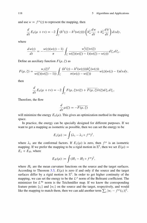
118 5 Algorithms and Applications
and use w D f �.z/ to represent the mapping, then
d
dtEh.�C t�/ D �2
ZC
.h1.z/ � h2.w.z///�h2wdw
dtC h2Nw
d Nwdt
�dxdy;
where
dw.z/
dtD �w.z/.w.z/ � 1/
�
ZC
w2z .�/�.�/
w.�/.w.�/ � 1/.w.�/ � w.z//d�xd�y:
Define an auxiliary function F.�; �/ as
F.�; �/ D wz.�/2
w.�/.w.�/ � 1//ZC
.h1.z/ � h2.w.z///h2w.w.z//�.w.z/ � w.�//
w.z/.w.z/ � 1/dxdy;
then
d
dtEh.�C t�/ D �2
ZC
F.�; �/�.�/C F.�; �/ N�.�/d�xd�y:
Therefore, the flow
d
dt�.�/ D �F.�; �/
will minimize the energy Eh.�/. This gives an optimization method in the mappingspace.
In practice, the energy can be specially designed for different purposes. If wewant to get a mapping as isometric as possible, then we can set the energy to be
E�.�/ WDZ.�1 � �2 ı f �/2;
where �k are the conformal factors. If E�.�/ is zero, then f � is an isometricmapping. If we prefer the mapping to be a rigid motion in E
3, then we set E.�/ DE� CEH , where
EH.�/ WDZ.H1 �H2 ı f �/2;
where Hk are the mean curvature functions on the source and the target surfaces.According to Theorem 3.3, E.�/ is zero if and only if the source and the targetsurfaces differ by a rigid motion in E
3. In order to get higher continuity of themapping, we can set the energy to be the Lp norm of the Beltrami coefficient. Theminimizer for L1 norm is the Teichmüller map. If we know the correspondingfeature points fzig and fwig on the source and the target, respectively, and wouldlike the mapping to match them, then we can add another term
Pi jwi � f �.zi /j2.

5.2 Registration and Tracking 119
Fig. 5.6 Quasi-conformal registration for a topological annulus case. The ellipse field on thesource domain (a) is mapped to the circle field on the target domain (b). The distortion is visualizedby the eccentricity of ellipsesD.�/ on both the 3D surface and its circle domain (c), where the redcolor denotes the higher non-conformality and the blue color denotes the higher conformality
Application
Registration of Surfaces with Large Deformations. Quasi-conformal geometryprovides a powerful approach to registration. The strategy for registration is first toestimate the Beltrami coefficient � and then compute the quasi-conformal mappingunder the auxiliary metric associated with �. A coarse-to-fine method to compute� was introduced in [21]. The Beltrami coefficient is estimated from the graph offeature points, then refined by the diffusion on the whole surface. The Beltramicoefficient can also be obtained by minimizing the matching energy [13]. Themethods can handle surfaces with complicated topologies and large anisometricdeformations.
Figure 5.6 shows the registration between two facial surfaces of the sameperson with a large expression deformation. Both faces are mapped to the planarannuli conformally, then the annuli are registered by a quasi-conformal mappingusing the auxiliary metric method. The consistent circle packing texture mappingdemonstrates the one-to-one correspondence between two faces. From the figure,we can see that an ellipse field on the calm face is mapped to a circle fieldon the frightened face, therefore, the mapping is quasi-conformal. The distortioncan be visualized by the color encoded eccentricity and argument of the Beltramicoefficient.

120 5 Algorithms and Applications
Fig. 5.7 Colon wall surface flattening by Euclidean Ricci flow. The rectangular flattened mappingis cut to three segments for display. Data courtesy of Arie E. Kaufman
Virtual Colonoscopy. Colorectal cancer is the third most incident cancer andthe second leading cause of cancer-related mortality in the USA [8]. Opticalcolonoscopy (OC), whereby precancerous polyps can be located and removed, hasbeen recommended for screening and has helped to greatly reduce the mortality rateof colorectal cancer [1]. Virtual colonoscopy (VC) techniques have been developedas viable noninvasive alternatives to OC for screening purposes [7, 11]. The colonwall surface is reconstructed from CT images. By using Ricci flow, one can flattenthe whole colon wall surface onto a planar rectangle [15]. Then polyps and otherabnormalities can be found efficiently on the planar image by Computer AidedDetection (CAD) techniques.
For a VC procedure, CT scans of the abdomen are commonly acquired with thepatient in both supine (facing up) and prone (facing down) positions. Being ableto register these two scans is useful for a routine VC system to provide the userwith ability for confirming a finding or easy comparison when something might beunclear in one of the scans, and is also helpful for a CAD system to achieve greateraccuracy while at the same time reducing false positive results. As shown in Fig. 5.7,the colon surface is regarded as a topological cylinder, therefore can be mapped toa rectangle using Euclidean Ricci flow. By quasi-conformal registration, we obtainthe one-to-one correspondence between them, then use that to analyze and visualizethe elastic deformation of the colon. Details can be found in [27].
Human Facial Expression Deformation. Different human facial expressions havedifferent deformation patterns, therefore, different types of Beltrami coefficients.We can do clustering in the Beltrami coefficient space for human facial expressionanalysis and recognition [21].
Brain Morphology. Neuroscientists commonly aim to identify abnormal defor-mations of cortical and subcortical structures in the brain in order to detectsystematic patterns of alterations in brain diseases. The normal deformations ofa brain cortical surface are isotropic, namely, nearly conformal. Some diseaseswill cause anisotropic deformations at some regions. Then for areas with isotropicdeformations, the norm of Beltrami coefficient � is close to zero; for areas withanisotropic deformation, � has greater norms. For example, the norm of � is a goodindicator for the gyral thickening on the cortical surface.

5.3 Shape Analysis 121
This method can be generalized to monitor the progression of neuron diseasesby qualitatively measuring the degree of abnormalities using the time-dependentBeltrami coefficients�.t/. We reconstruct a sequence of cortical surfaces S.t/ of thesame patient from regular MRI scans, and register S.t/ to the initial surface S.0/.The Beltrami coefficient of the mapping is denoted as �.t/. By analyzing �.t/,we can monitor the shape deformations and estimate the severity of abnormalities.Details can be found in [12].
5.3 Shape Analysis
The purpose of shape analysis is to classify shapes, compare shapes, quantifytheir similarities and differences, and measure the distances between shapes. Onesystematic way to perform shape analysis is to construct the shape space, which is aninfinite dimensional Riemannian manifold. Each point in the shape space representsa shape, or a class of shapes; a curve represents a deformation process from oneshape to the other. The Riemannian metric is used to measure the distances andcompute geodesics, where geodesics represent the most natural deformation fromthe source to the target.
In the following discussion, we focus on three models of shape space:
1. 2D planar shape space based on conformal welding theory: The planar contoursare converted to the diffeomorphism space of the unit circle, and the distancebetween shapes is measured using the Weil–Petersson metric. The basic ideais straightforward. A planar contour segments the whole plane to two connectedcomponents. Each of them is mapped to the unit disk via Riemann mapping. Thisinduces a homeomorphism between the boundaries of the two disks, namely, anautomorphism of the unit circle, which is called the “fingerprint” of the contour.Inversely, we can weld two disks using the fingerprint to fully recover the originalcontour. We can measure the distance between two contours by computing thenorm between their fingerprints. Details can be found in Sect. 5.3.1.
2. Teichmüller space for surfaces: All surfaces are classified by conformal equiv-alence relation. The coordinates of a shape is given by its conformal module.The distance is measured by Teichmüller metric. The conformal modules canbe computed using the Ricci flow method. The Teichmüller distance requiressolving the extremal quasi-conformal mapping problem. The method is elabo-rated in Sect. 5.3.2.
3. 3D surface space based on conformal representation: For surfaces embedded inR3, they are determined by the conformal factor, the mean curvature, and the
boundary conditions, uniquely up to a rigid motion. Then we can represent asurface by its conformal factor and mean curvature functions on the uniformiza-tion domain. This unified view greatly simplifies the task of shape analysis. Themethod is explained thoroughly in Sect. 5.3.3.

122 5 Algorithms and Applications
5.3.1 2D Shape Space Based on Conformal Welding
Ricci flow can be applied for modeling the 2D shape space based on conformalwelding theory. Suppose � D f�0; �1; : : : ; �ng is a set of nonintersecting smoothclosed curves on the complex plane. � segments the plane to a set of connectedcomponents f˝0;˝1; : : : ; ˝nC1g. Each segment ˝k may be a simply connecteddomain or a multiply connected domain.
We assume ˝nC1 contains the infinity point. Select one point p outside ˝nC1,p 62 ˝nC1. By using a Möbius transformation, �.z/ D 1=.z�p/, p is mapped to 1,and ˝nC1 is mapped to a compact domain. Replace ˝nC1 by �.˝nC1/. Constructconformal mappings using Ricci flow, �k W ˝k ! Dk , to map each segment ˝k
to a circle domain Dk , 0 � k � n C 1. We denote the conformal module of Dk
as Mod.Dk/, which is also the conformal module of ˝k , Mod.˝k/. Assume �k 2� D ˝i \˝j . Then �i .�k/ is a circular boundary C i
k of the circle domain Di , and
�j .�k/ is also a circular boundary Cj
k of Dj . Let fk WD �i ı ��1j jS1 W S1 ! S1 be
the diffeomorphism from the circle S1 to itself, which is called the signature of �k .
Definition 5.1 (Conformal Welding Signature of a Family of Planar Curves).The signature of a family of nonintersecting closed planar curves � Df�0; �1; : : : ; �ng is defined as S.� / WD ff0; f1; : : : ; fng[fMod.D0/;Mod.D1/; : : : ;
Mod.DnC1/g.
Theorem 5.1 (Conformal Welding of Planar Closed Curves [14]). The family ofsmooth planar closed curves � is determined by its signature S.� /, uniquely up toa Möbius transformation of the Riemann sphere C [ f1g.
Proof. Let˝k be one segment, which is conformally mapped to a circle domainDk .Assume two segments ˝i and ˝j share a common boundary �k , �k D ˝i \ ˝j .We can glue Di and Dj using the signature of �k . Namely, a boundary point p 2@˝i is equivalent to q 2 @˝j , p � q, if and only if q D fk.p/. Then we glue allthe circle domains to get a Riemann surface
R WD[k
Dk= � :
R is a topological sphere with a conformal structure. Then by uniformizationtheorem, it can be equipped with the spherical metric. The unit sphere is conformallymapped to the extended complex plane NC. By a Möbius transformation, the imagesof the boundaries of Dk’s coincide with �k’s. ut
The theorem states that the conformal welding signature determines 2D shapesuniquely up to a Möbius transformation. The shape signature S.� / gives us acomplete representation for the 2D shape. Therefore the 2D shape space can bemodeled as the space of all conformal welding signatures. Furthermore, we can alsodefine a Riemannian metric for the 2D shape space, such as the Weil–Peterssonmetric [16].

5.3 Shape Analysis 123
D0D1
D2Ω2
Ω1
Ω0
γ2
γ1
γ0
C20
C10
C0
C11
C21
a
cb
c0 =(0,0)c1 =(0,0)c2 =(0,0.7757)r0 =1r1 =0.2415r2 =0.2520
f2
f1
0 1 2 3 4 5 60
1
2
3
4
5
6
Fig. 5.8 Conformal welding signature. (a) Each segment is mapped to a circle domain. (b)The conformal modules (centers and radii of inner circles) of the circle domains and thediffeomorphisms of the circles define the signature. (c) The shape can be reconstructed from thesignature
We demonstrate the process for computing the conformal welding signaturewith a double fish image as shown in Fig. 5.8. Given the original image, we firstperform image segmentation, then calculate the contours of the segments in theimage. For simplicity, we treat the outermost boundary of the image as the unitcircle. Then all the contours segment the image to planar domains ˝0;˝1;˝2.We conformally map each planar domain to a circle domain, ˚i W ˝i ! Di . ˝0
is mapped to a disk D0 with two circular holes. The centers and radii .c0; r0/ and.c1; r1/ form the conformal module of ˝0. Also, ˝1 and ˝2 are mapped to the unitdisks D1 and D2, respectively. The contour �1 of the small fish is mapped to theboundary C1
1 of D1 and one inner boundary C01 of D0. The signature is given by
f1 WD ˚1 ı ˚�10 . Similarly, the signature f2 of the contour of the shark can also becomputed. The signature of both contours is given by S.� / D fc0; c1; r1; r2; f1; f2g.The computational steps are shown in Algorithm 5.9. The planar shapes can bereconstructed from the signature through the combinatorial operations as describedin Algorithm 5.10.

124 5 Algorithms and Applications
Algorithm 5.9 Conformal welding signature of planar shapesInput: A planar triangular mesh ˝ with one exterior boundary �0 and n inner contours f�k; k D
1; : : : ; ng, which decompose ˝ into nC 1 sub-domains f˝k; k D 0; 1; : : : ; ng.Output: Conformal welding signature
S.� / WD ff1; : : : ; fng [ fMod.˝0/;Mod.˝1/; : : : ;Mod.˝n/g:1: for all sub-domain ˝k do2: Compute the conformal map from ˝k to circle domains Dk , �k W ˝k ! Dk .3: end for4: for all sub-domain ˝k do5: Compute the conformal module Mod.˝k/ of Dk .6: end for7: for all inner boundary �k D ˝i \˝j do8: Compute the signature of �k , fk D �i ı ��1
j .9: end for
Algorithm 5.10 Planar shape reconstruction from conformal welding signatureInput: Conformal welding signature: the automorphisms of circles ff1; : : : ; fng and the confor-
mal modules fMod.D0/;Mod.D1/; : : : ;Mod.Dn/g.Output: Planar contours � .1: for all conformal module Mod.Dk/ do2: Construct circle domain Dk directly from its module Mod.Dk/.3: Use Delaunay refinement algorithm to compute the meshing of Dk .4: end for5: for all circle automorphism fk do6: Assume �k D ˝i \˝j . Combinatorially glue the triangular mesh Di and Dj by fk . For
each vertex vi 2 @Di , insert fk.vi / to @Dj ; vice versa, for each vertex vj 2 @Dj , insertf �1k .vj / to @Di .
7: Use constrained Delaunay triangulation to refine the triangulation of Di and Dj .8: Glue the refined triangle mesh Di and Dj combinatorially by fk .9: end for
10: Run Ricci flow algorithm to compute a spherical metric for the glued mesh R.11: Conformally map R to the complex plane using stereo-graphic projection. Normalize the
mapping by a Möbius transformation.
Application
2D Shape Indexing and Retrieval. Shape analysis of objects from their observedsilhouettes is important for many computer vision applications, such as classifica-tion, recognition, and image retrieval. In real world applications, objects from theirobserved silhouettes are usually multiply connected domains, i.e., domains withholes in the interior. Most of the existing methods work only on simple closed curvesand generally cannot deal with multiply connected objects. Sharon and Mumford[16] proposed a conformal approach to model simple closed curves which capturessubtle variability of shapes uniquely up to scalings and translations. They alsointroduced the Weil–Petersson metric on their proposed shape space. The methodis generalized to represent multiple objects in a single image (i.e., with multiple

5.3 Shape Analysis 125
c0 = (0,0)r1 = 0.5773c1 = (0,0)r2 = 0.2776
c0 = (0,0)
r2 = 0.4021
c1 = (0,0)
r2 = 0.4029
c0 = (0,0)
r1 = 0.6949
c1 = (0,0)
r2 = 0.4915
f1
6
f2f1
f1
f2
f2
γ0
γ1
γ2
γ0
γ1
γ2
γ0
γ1
γ2
5
4
3
2
1
00 1 2 3 4 5 6
6
5
4
3
2
1
00 1 2 3 4 5 6
6
5
4
3
2
1
00 1 2 3 4 5 6
Fig. 5.9 Conformal welding shape signatures of three different images with two levels of contours
contours) based on conformal welding signatures in [14]. The shape signature iscomplete and can represent 2D shapes with arbitrary topologies uniquely up toscalings and translations. As shown in Fig. 5.9, the three different images withmultiple boundaries have very different shape signatures. This demonstrates thatthe representation can be used to effectively classify 2D shapes.
Brain Morphology. The conformal welding idea can be extended from 2D shapespace to 3D shape space, by combining conformal modules and curve diffeomor-phism signatures to form 3D conformal welding signatures [29]. It describes theshape and location of 3D simple and nonintersecting contours on the embeddingsurface, and the underlying geometric correlation between each patches. It hasbeen successfully used for classifying the human brain cortical surfaces among thehealthy control group and the Alzheimer’s Disease (AD) group. The structural MRIdata were obtained from the Alzheimer’s Disease Neuroimaging Initiative (ADNI)database (www.adni.loni.ucla.edu). In the computation, the brain cortical surfaceis partitioned into different functional regions, each region is conformally mappedto a canonical circle domain. This can be accomplished by using the Euclideandiscrete Ricci flow method [9, 18, 28] as described in Algorithms 5.11 and 5.12.Then the boundary of each region induces a diffeomorphism from the unit circleto itself. The shapes of canonical spaces and the automorphisms of the unit circleform the signature as shown in Fig. 5.10. Theoretically, the signature is guaranteedto be a complete and global shape descriptor based on Teichmüller space theoryand conformal welding theory. This method focuses on both local geometries of

126 5 Algorithms and Applications
Algorithm 5.11 Conformal module for doubly connected annuliInput: A triangular mesh M , which is a doubly connected annulus.Output: Conformal module of M .1: Set target curvature equal to zero everywhere.2: Compute a flat metric using Euclidean Ricci flow in Algorithm 5.2.3: Compute the shortest path � between two boundaries.4: Slice the M along � to get NM .5: Flatten NM onto the plane using Euclidean embedding in Algorithm 5.4.6: Scale and translate the planar image of NM , such that the image of the outer boundary is aligned
with the imaginary axis, the length of outer boundary is 2� .7: Use the exponential map z! ez to map the planar image of NM to an annulus.8: Measure the radii of inner and outer boundary circles r and R, respectively. The conformal
module is given by 12�
ln Rr
.
Algorithm 5.12 Conformal module for triply connected annuli by Euclidean Ricciflow (generalized Koebe’s method)Input: A triangular mesh M , which is a triply connected annulus, with boundaries @M D �0 �
�1 � �2.Output: The Euclidean conformal module of M .1: repeat2: Fill �1 by a topological disk, to get M1.3: Use Algorithm 5.11 to map M1 to a canonical planar annulus QM1.4: On QM1, remove the hole of �1 and fill the hole �2 to get M2.5: Use Algorithm 5.11 to map M2 to a canonical planar annulus QM2.6: On QM2, remove the hole of �2, to get QM .7: M QM .8: until The curvatures on the boundaries are close to constants9: Suppose the center of �1 is z0. Define a Möbius transformation z ! z�z0
1�Nz0z to map the centerof �1 to the origin.
10: Rotate the planar image, such that the center of �2 is on the imaginary axis.
functional regions and global geometric relations among them. The local-globalview based on conformal geometry would be highly advantageous for biomarkerresearch in AD.
5.3.2 Teichmüller Space
According to Theorem 3.1, all surfaces in real world are Riemann surfaces, thereforehave conformal structures. All metric surfaces in real world can be classified byconformal equivalence. The space of all conformal classes is the Teichmüller space.The Teichmüller space coordinates are given by conformal modules, which are thecomplete invariants of conformal structures and intrinsic to surfaces themselves.The Teichmüller space coordinates can be applied for shape indexing directly.
The representations for the conformal module of a surface are not unique. Onerepresentation is based on Euclidean Ricci flow. The other is based on hyperbolic

5.3 Shape Analysis 127
γ1
S1S3
S2D1
D3D2
D0
c1
c3
c2
γ3
γ1
γ3
γ2
γ2
c1 = (0,0) r1 = 1
c2 = (0,0) r2 = 0.0423
c3 = (0,0.1368) r3 = 0.0635
θ2
θ10
01
1
2
2
3
3
4
4
5
5
7
7
6
6
ab
c d
Fig. 5.10 Conformal welding signature via uniformization mapping for a hemisphere brainsurface with 3 simple closed contours. The curve �i (a) surrounds the patch Si (c) and is mappedto the boundary ci of the circle domainDi (c). �i is also mapped to the boundary of the base circledomain D0 (b). The curves (d) demonstrate the diffeomorphisms for the three contours
Ricci flow. A topological multiply connected annulus, i.e., a genus zero surface withmultiply boundaries, can be mapped to the canonical circle domain using EuclideanRicci flow. Two circle domains are conformally equivalent if and only if they differby a Möbius transformation. Suppose the boundaries of a circle domainD are @D DC0 �C1 �C2 � � � � �Cn, where Ck is a circle with the center ck D .xk; yk/ and theradius rk , denoted as .ck; rk/. One can normalize D by a Möbius transformation,such that C0 becomes the unit circle, c1 is at the origin, and c2 is on the imaginaryaxis. Then the normalized circle domain is determined by Mod.D/ D fr1; y2; r2g [fxk; yk; rk; k > 2g, which is called the conformal module of the circle domain.Algorithms 5.11 and 5.12 explain the details for computing conformal module fordoubly and triply connected annuli using Euclidean Ricci flow and the generalizedKoebe’s method [30, 31]. The proof for the convergence of the Koebe’s algorithmcan be found in [5].
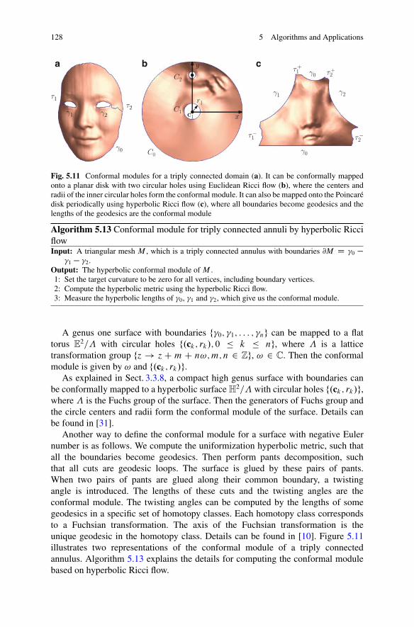
128 5 Algorithms and Applications
γ0
γ1 γ2
τ1τ2
γ0
γ0
γ1 γ2
τ1+
τ1−
τ2+
τ2−
a c
r1
c1 x
y
C0
C2
C1
b
Fig. 5.11 Conformal modules for a triply connected domain (a). It can be conformally mappedonto a planar disk with two circular holes using Euclidean Ricci flow (b), where the centers andradii of the inner circular holes form the conformal module. It can also be mapped onto the Poincarédisk periodically using hyperbolic Ricci flow (c), where all boundaries become geodesics and thelengths of the geodesics are the conformal module
Algorithm 5.13 Conformal module for triply connected annuli by hyperbolic RicciflowInput: A triangular mesh M , which is a triply connected annulus with boundaries @M D �0 �
�1 � �2.Output: The hyperbolic conformal module of M .1: Set the target curvature to be zero for all vertices, including boundary vertices.2: Compute the hyperbolic metric using the hyperbolic Ricci flow.3: Measure the hyperbolic lengths of �0, �1 and �2, which give us the conformal module.
A genus one surface with boundaries f�0; �1; : : : ; �ng can be mapped to a flattorus E
2= with circular holes f.ck; rk/; 0 � k � ng, where is a latticetransformation group fz ! z C m C n!;m; n 2 Zg, ! 2 C. Then the conformalmodule is given by ! and f.ck; rk/g.
As explained in Sect. 3.3.8, a compact high genus surface with boundaries canbe conformally mapped to a hyperbolic surface H2= with circular holes f.ck; rk/g,where is the Fuchs group of the surface. Then the generators of Fuchs group andthe circle centers and radii form the conformal module of the surface. Details canbe found in [31].
Another way to define the conformal module for a surface with negative Eulernumber is as follows. We compute the uniformization hyperbolic metric, such thatall the boundaries become geodesics. Then perform pants decomposition, suchthat all cuts are geodesic loops. The surface is glued by these pairs of pants.When two pairs of pants are glued along their common boundary, a twistingangle is introduced. The lengths of these cuts and the twisting angles are theconformal module. The twisting angles can be computed by the lengths of somegeodesics in a specific set of homotopy classes. Each homotopy class correspondsto a Fuchsian transformation. The axis of the Fuchsian transformation is theunique geodesic in the homotopy class. Details can be found in [10]. Figure 5.11illustrates two representations of the conformal module of a triply connectedannulus. Algorithm 5.13 explains the details for computing the conformal modulebased on hyperbolic Ricci flow.

5.3 Shape Analysis 129
Application
Human Facial Surface Indexing. We capture 3D faces of different persons withthe same expression. Then we extract the contours of the mouth and both eyes andremove the interior regions, making the surfaces into multiply connected domains,i.e., genus zero surfaces with four boundaries. We apply Euclidean Ricci flow to mapthe surface onto the unit disk with circular holes. Let the centers of the circular holesbe ck=.xk; yk/, k D 0; 1; 2; 3 and the radii be rk . We use a Möbius transformationto normalize the mapping such that the exterior circle becomes a unit circle, thefirst inner circle is centered at the origin, and the center of the second circle is onthe positive side of the imaginary axis, i.e., r0 D 1, .x0; y0/ D .0; 0/, .x1; y1/ D.0; 0/, and x2 D 0, similar to the normalization in Fig. 5.11b. Then the conformalmodule is given by .r1; y2; r2; x3; y3; r3/. The Teichmüller space is 6 dimensional.Conformal modules can be used for 3D human face shape indexing. Details can befound in [28].
Vestibular System Morphometry. Adolescent Idiopathic Scoliosis (AIS) character-ized by 3D spine deformity affects about 4 % schoolchildren worldwide. One ofthe prominent theories of the etiopathogenesis of AIS was proposed to be thepoor postural balance control due to the impaired vestibular function. Thus, themorphometry of the vestibular system (VS) is of great importance for studying AIS.The VS is a genus three structure situated in the inner ear and consists of threesemicircular canals lying perpendicular to each other. The high genus topologyof the surface poses great challenge for shape analysis. An effective method isto analyze shapes of high genus surfaces by considering their geodesic spectra.The key is to compute the canonical hyperbolic geodesic loops of the surface,using hyperbolic Ricci flow, as shown in Fig. 5.12. The geodesic spectra effectivelymeasure shape differences between high genus surfaces up to hyperbolic isometry.Experimental results on the VS of normal and AIS subjects show the effectiveness ofthe algorithm and reveal the statistical shape difference between two groups. Detailscan be found in [24].
Brain Mapping. The human brain cortical surfaces can be reconstructed fromCT images and discretized as triangular meshes. The brain cortical surface, atopological sphere, can be mapped to a unit sphere, as shown in Fig. 3.4. All thegeometric details are exposed onto the sphere. The morphometry analysis can beconstructed on the canonical domain. Besides that, by using the landmarks onthe brain, the brain surface is sliced open with holes, where each landmark generatesa hole. Therefore, the brain cortical surface with holes can be either mapped toa circle domain where each hole is mapped to a circle, or a hyperbolic convexdomain where each hole is mapped to a geodesic in hyperbolic space. The conformalmodules can be extracted for brain surface shape analysis purposes. Figure 5.13shows an example of hyperbolic mapping for a brain cortical surface with oneboundary and three interior landmarks.

130 5 Algorithms and Applications
a1
b1
b3
b2
a2
a3
a1
b1
a2
b2
a3
b3
a b
Fig. 5.12 Computing the geodesic loops for each homotopy class of a VS surface. All the geodesicloops fai ; big; i D 1; 2; 3 (a) form the homotopy group basis on the Poincaré disk (b). The lengthsof the geodesic loops in R
3 form the geodesic spectra
γ1
γ2
γ3
τ3
τ2
τ1
γ0
τ3
τ2
τ1
τ2+
τ1+
γ012
γ2
γ1
γ3
γ023 τ2
−τ3
+
γ031 τ3
−τ1
+
a b c
Fig. 5.13 Brain mapping by hyperbolic Ricci flow. A human brain surface with one boundary�0 (b) is sliced open by three interior landmarks �k; k D 1; 2; 3 (a), then it becomes a genuszero surface with four boundaries. By hyperbolic Ricci flow, it is mapped to a hyperbolic convexpolygon on Poincaré disk (c) where the domain is sliced open by three curves �k (b) between �0and �k , respectively
It is crucial to register different brain cortical surfaces in brain imaging field.Since brain cortical surfaces are highly convoluted and different people havedifferent anatomic structures, it is quite challenging to find a good registration (ormapping) between them. By finding an automorphism of the canonical shapes, theregistration between surfaces can be easily established. The computation of thespherical, Euclidean, and hyperbolic brain mappings is based on the discrete Ricciflow method, as described in Algorithm 5.2. The details of brain surface mappingand its applications can be found in [3, 18].
Human Facial Surface Dynamics Analysis. Suppose a sequence of facial surfaceswith different expression changes are captured. By computing the time-dependent

5.3 Shape Analysis 131
Fig. 5.14 Conformal modules of a sequence of human facial surfaces with dynamic expressions.All the faces are mapped to a unit disk with one concentric circle with radius r . The conformalmodule is defined as 1
2�ln 1
r, which decreases monotonically as the inner circle radius increases
conformal module R.t/, we can analyze the expression. Figure 5.14 shows such anexample. A sequence of male facial surfaces from calm expression to frightenedexpression is acquired using 3D camera system [17]. We remove the mouth regionand compute the conformal module. It is easy to see that the human facial expressionintensity is proportional to the norm of the conformal module. Details can be foundin [20].
5.3.3 Surface Conformal Representation
According to Theorem 3.3, a surface embedded in R3 is fully determined by the
conformal factor function � and the mean curvature function H defined on theconformal structure R, then we use .R; �;H/ as the representation of the surface.R gives the Riemann surface structure, .R; �/ gives the Riemannian metric, and.R; �;H/ gives the embedding of the surface in R
3. The Riemann surface R can berepresented using its conformal module.
Given a surface S embedded in R3, it has the induced Euclidean metric g.
We compute its uniformization metric g0 using Ricci flow and obtain the Riemannsurface structure R and the conformal factor g D e2�g0. We choose local conformalparameters z of R. The mean curvature is computed as

132 5 Algorithms and Applications
DI03AN03 FE03 HA03 SA03 SU03
Fig. 5.15 Conformal representations for 3D human facial surfaces with expressions with the 3rdintensity level. The subject is M0021 in BU3D database. From upper to bottom: human face imagesin camera view, conformal maps with human facial textures, mean curvature images, and conformalfactor images for 6 expressions, respectively
H.z/ D�4
e2�.z/@2r.z/@z@Nz ;n.z/
;
where r.z/, n.z/ are the position vector and the normal of the surface, respectively.Figure 5.15 illustrates the conformal representations of a 3D human facial surfacewith 6 different expressions. Each column gives the conformal representation for adifferent expression. From upper to bottom, the first row shows the original surfacewith texture, the second row is the image of conformal mapping, and the third andthe fourth rows show the conformal factor and the mean curvature functions definedon the conformal parameter domain, respectively, which are color encoded as gray-level images. Details can be found in [23].
Measuring the distance among shapes has fundamental importance in practice.In the following, we give one way to define shape distance between two surfacesbased on their conformal representations and the diffeomorphic registration betweenthem. Given two surfaces .S1; g1/ and .S2; g2/, we compute their conformalrepresentations using Ricci flow, .R1; �1;H1/ and .R2; �2;H2/. Then we can definethe distance between them as

5.3 Shape Analysis 133
d.S1; S2/ WD minf WR1!R2
�ZR1
.�1 � �2 ı f /2� 12
C�Z
R1
.H1 �H2 ı f /2� 12
;
where we restrict the mapping f to be a diffeomorphism. It is straightforward toshow that d.�; �/ satisfies the triangle inequality.
The optimal diffeomorphism f W R1 ! R2 can be obtained using quasi-conformal geometric method introduced in Sect. 5.2.3. If we emphasize the effi-ciency, then the mapping f could be chosen to be harmonic mappings. If thesurfaces are with negative Euler number, then we can equip the target with thehyperbolic metric, under which the harmonic mapping is unique in each homotopyclass and can be computed using the method introduced in Sect. 5.2.2.
Application
3D Human Facial Expression Recognition. Surface conformal representation canbe applied for 3D human facial expression recognition. An automatic 3D expressionrecognition system has been built up and tested on the BU3D database [19]. Foreach subject, the database includes one neutral and six prototypical non-neutralexpressions, such as happiness (HA), sadness (SA), anger (AN), fear (FE), surprise(SU), and disgust (DI), with four intensity levels. As shown in Fig. 5.15,the confor-mal representations for all facial surfaces are automatically computed and classifiedusing standard classifiers. The preliminary experimental results show the currentapproach is highly competitive [23].
Symmetry Detection. Symmetry analysis is an important task in shape analysis.There are intrinsic symmetry and extrinsic symmetry. Suppose .S; g/ is a metricsurface. A mapping f W S ! S is isometric if the pullback metric equals theoriginal metric, g D f �g. All the isometric automorphisms of S form a group,which is the intrinsic symmetry group of the surface. Furthermore, if an isometricautomorphism f also preserves mean curvature, namely, H ı f D H , then f isalso an extrinsic symmetry.
Ricci flow can help detect such type of symmetry. The key observation is thatRicci flow preserves intrinsic symmetry. Suppose g.t/ is the Riemannian metricduring the flow at time t . If an automorphism f W S ! S is isometric at thebeginning, f �g.0/ D g.0/, then for all time t , f �g.t/ D g.t/. Let t ! 1,then g.1/ is one of the three canonical metrics, spherical, Euclidean, or hyperbolicmetric. Then the intrinsic symmetry group must be a subgroup of the rigid motiongroup under the canonical metric.
Furthermore, the symmetry axis or the fixed point sets of the isometric mappingf , fp 2 S jf .p/ D pg, must be geodesics. The geodesics under canonicalmetrics are spherical, Euclidean, or hyperbolic lines. Therefore, by using Ricciflow, intrinsic symmetry detection can be carried out in a much easier way.Figure 5.16 demonstrates the symmetry on both the original surface and theconformal parameter domain obtained by the Ricci flow method.
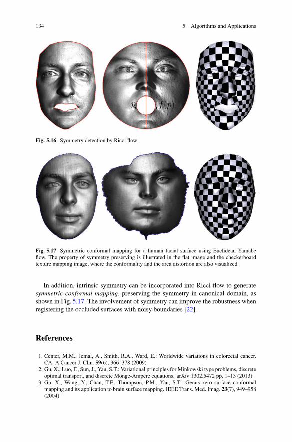
134 5 Algorithms and Applications
Fig. 5.16 Symmetry detection by Ricci flow
Fig. 5.17 Symmetric conformal mapping for a human facial surface using Euclidean Yamabeflow. The property of symmetry preserving is illustrated in the flat image and the checkerboardtexture mapping image, where the conformality and the area distortion are also visualized
In addition, intrinsic symmetry can be incorporated into Ricci flow to generatesymmetric conformal mapping, preserving the symmetry in canonical domain, asshown in Fig. 5.17. The involvement of symmetry can improve the robustness whenregistering the occluded surfaces with noisy boundaries [22].
References
1. Center, M.M., Jemal, A., Smith, R.A., Ward, E.: Worldwide variations in colorectal cancer.CA: A Cancer J. Clin. 59(6), 366–378 (2009)
2. Gu, X., Luo, F., Sun, J., Yau, S.T.: Variational principles for Minkowski type problems, discreteoptimal transport, and discrete Monge-Ampere equations. arXiv:1302.5472 pp. 1–13 (2013)
3. Gu, X., Wang, Y., Chan, T.F., Thompson, P.M., Yau, S.T.: Genus zero surface conformalmapping and its application to brain surface mapping. IEEE Trans. Med. Imag. 23(7), 949–958(2004)

References 135
4. Haber, E., Metaxas, D.N., Axel, L.: Motion analysis of the right ventricle from MRI images. In:International Conference on Medical Image Computing and Computer Assisted Intervention(MICCAI’98), Springer-Verlag, Berlin, Heidelberg, pp. 177–188 (1998)
5. Henrici, P.: Applied and Computational Complex Analysis, vol. 3. Wiley-Intersecience, NewYork (1988)
6. Hernandez, C., Vogiatzis, G., Brostow, G.J., Stenger, B., Cipolla, R.: Non-rigid photometricstereo with colored lights. In: IEEE International Conference on Computer Vision (ICCV’07),Institute of Electrical and Electronics Engineers (IEEE), pp. 1–8 (2007)
7. Hong, L., Muraki, S., Kaufman, A., Bartz, D., He, T.: Virtual Voyage: Interactive Navigationin the Human Colon. ACM SIGGRAPH, New York, pp. 27–34 (1997)
8. Horner, M.J., Ries, L.A.G., Krapcho, M., Neyman, N., Aminou, R., Howlader, N., Altekruse,S.F., Feuer, E.J., Huang, L., Mariotto, A., Miller, B.A., Lewis, D.R., Eisner, M.P., Stinchcomb,D.G. In: Edwards, B.K. (eds.) SEER Cancer Statistics Review, 1975–2006, National CancerInstitute, Bethesda, MD (2009)
9. Jin, M., Kim, J., Luo, F., Gu, X.: Discrete surface Ricci flow. IEEE Trans. Visual. Comput.Graph. 14(5), 1030–1043 (2008)
10. Jin, M., Zeng, W., Ding, N., Gu, X.: Computing Fenchel-Nielsen coordinates in Teichmüllershape space. Int. J. Commun. Inform. Syst. 9(2), 213–234 (2009)
11. Johnson, C.D., Dachman, A.H.: CT colography: the next colon screening examination.Radiology 216(2), 331–341 (2000)
12. Lui, L.M., Wong, T.W., Zeng, W., Gu, X., Thompson, P.M., Chan, T.F., Yau, S.T.: Detectingshape deformations using Yamabe flow and Beltrami coefficients. J. Inverse Prob. Imag. 4(2),311–333 (2010)
13. Lui, L.M., Wong, T.W., Zeng, W., Gu, X., Thompson, P.M., Chan, T.F., Yau, S.T.: Optimizationof surface registrations using Beltrami holomorphic flow. J. Scient. Comput. 50(3), 557–585(2012)
14. Lui, L.M., Zeng, W., Chan, T., Yau, S.T., Gu, X.: Shape representation of planar objects witharbitrary topologies using conformal geometry. In: European Conference on Computer Vision(ECCV’10), Crete, Greece (2010)
15. Qiu, F., Fan, Z., Yin, X., Kauffman, A., Gu, X.: Colon flattening with discrete Ricci flow. In:International Conference on Medical Image Computing and Computer Assisted Intervention(MICCAI’09), London, England (2009)
16. Sharon, E., Mumford, D.: 2D-shape analysis using conformal mapping. Int. J. Comput. Vision70, 55–75 (2006)
17. Wang, Y., Gupta, M., Zhang, S., Wang, S., Gu, X., Samaras, D., Huang, P.: High resolutiontracking of non-rigid motion of densely sampled 3d data using harmonic maps. Int. J. Comput.Vision 76(3), 283–300 (2008)
18. Wang, Y., Shi, J., Yin, X., Gu, X., Chan, T.F., Yau, S.T., Toga, A.W., Thompson, P.M.: Brainsurface conformal parameterization with the Ricci flow. IEEE Trans. Med. Imag. 31(2),251–264 (2012)
19. Yin, L., Wei, X., Sun, Y., Wang, J., Rosato, M.J.: A 3D facial expression database forfacial behavior research. In: IEEE International Conference on Automatic Face and GestureRecognition (FG’06), vol. 0, pp. 211–216. IEEE Computer Society, Los Alamitos (2006)
20. Zeng, W., Gu, X.: 3D dynamics analysis in Teichmüller space. In: ICCV Workshop onDynamic Shape Capture and Analysis Recognition (4DMOD’11), Barcelona, Spain (2011)
21. Zeng, W., Gu, X.: Registration for 3D surfaces with large deformations using quasi-conformalcurvature flow. In: IEEE Conference on Computer Vision and Pattern Recognition (CVPR’11).Colorado Springs, Colorado (2011)
22. Zeng, W., Hua, J., Gu, X.: Symmetric conformal mapping for surface matching and registra-tion. Int. J. CAD/CAM 9(1), 103–109 (2009)
23. Zeng, W., Li, H., Chen, L., Morvan, J.M., Gu, X.: An automatic 3D expression recognitionframework based on sparse representation of conformal images. In: IEEE InternationalConference on Automatic Face and Gesture Recognition (FG’13). IEEE Computer Society,Shanghai (2013)

136 5 Algorithms and Applications
24. Zeng, W., Lui, L., Shi, L., Wang, D., Chu, W.C., Cheng, J., Hua, J., Yau, S.T., Gu, X.: Shapeanalysis of vestibular systems in adolescent idiopathic scoliosis using geodesic spectra. In:International Conference on Medical Image Computing and Computer Assisted Intervention(MICCAI’10), Beijing, China (2010)
25. Zeng, W., Lui, L.M., Luo, F., Chan, T., Yau, S.T., Gu, X.: Computing quasiconformal mapsusing an auxiliary metric with discrete curvature flow. Numeriche Mathematica 121(4),671–703 (2012)
26. Zeng, W., Luo, F., Yau, S.T., Gu, X.: Surface quasi-conformal mapping by solving Beltramiequations. In: IMA International Conference on Mathematics of Surfaces XIII, Springer-Verlag, Berlin, Heidelberg, pp. 391–408 (2009)
27. Zeng, W., Marino, J., Gurijala, K., Gu, X., Kaufman, A.: Supine and prone colon registrationusing quasi-conformal mapping. IEEE Trans. Visualiz. Comput. Graph. 16(6), 1348–1357(2010)
28. Zeng, W., Samaras, D., Gu, X.D.: Ricci flow for 3D shape analysis. IEEE Trans. Pattern Anal.Mach. Intell. 32(4), 662–677 (2010)
29. Zeng, W., Shi, R., Wang, Y., Yau, S.T., Gu, X.: Teichmüller shape descriptor and its applicationto Alzheimer’s disease study. Int. J. Comput Vision. 105(2), 155–170 (2013)
30. Zeng, W., Yin, X., Zhang, M., Luo, F., Gu, X.: Generalized Koebe’s method for conformalmapping multiply connected domains. In: SIAM/ACM Joint Conference on Geometric andPhysical Modeling (SPM’09), San Francisco, California (2009)
31. Zhang, M., Li, Y., Zeng, W., Yau, S.T., Gu, X.: Canonical conformal mapping for high genussurfaces with boundaries. Int. J. Comput. & Graph. 36(5), 417–426 (2012)

Index
Aadmissible curvature space, 76admissible metric space, 76area element, 2area preserving mapping, 7auxiliary metric, 46, 116, 117
BBeltrami coefficient, 45, 115Beltrami coefficient space, 117Beltrami differential, 47Beltrami equation, 116Beltrami holomorphic flow, 117biholomorphic function, 32biholomorphic mapping, 33boundary operator, 60brain mapping, 129
Ccanonical fundamental group basis, 19circle packing metric, 68Codazzi equation, 21conformal atlas, 32conformal factor, 7, 118conformal mapping, 7, 33conformal module, 14, 35, 126conformal structure, 32conformal surface representation, 48conformal transformation group, 12conformal welding, 122, 125connected sum, 17cosine law, 3cotangent weight, 109covering space, 19curvature evolution equation, 29
curvature map, 76cut graph, 103
Ddeck transformation, 20deck transformation group, 20deformable surface tracking, 108deformation field, 117derivative cosine law, 68diffeomorphism, 6Dirichlet boundary condition, 109discrete conformal equivalence, 68discrete conformal factor, 68discrete conformal structure, 86discrete curvature, 62discrete Gauss–Bonnet, 63discrete harmonic function, 110discrete hyperbolic Ricci energy, 95discrete Laplace-Beltrami operator, 110discrete Ricci energy, 74discrete Riemannian metric, 61discrete surface, 59double covering, 114dynamic shape tracking, 115
Eedge weight, 74Euclidean Ricci flow, 103extended complex plane, 42, 49, 117
Fface registration, 115facet, 60facial expression recognition, 133
W. Zeng and X.D. Gu, Ricci Flow for Shape Analysis and Surface Registration,SpringerBriefs in Mathematics, DOI 10.1007/978-1-4614-8781-4,© Wei Zeng, Xianfeng David Gu 2013
137

138 Index
first fundamental form, 22flat torus, 111Fricke coordinates, 42Fuchs group, 41, 128Fuchsian transformation, 41fundamental domain, 20, 104fundamental group, 19
GGauss curvature, 23Gauss equation, 21Gauss map, 111Gauss-Bonnet, 24generalized Koebe’s method, 127geodesic, 3geodesic curvature, 23geometric structure, 13
Hharmonic map, 51, 109, 112heat flow, 52holomorphic differential 1-form, 33holomorphic function, 31holomorphic quadratic differential, 33, 57homeomorphism, 6homeomorphism group, 11homotopy, 18Hopf differential, 54hyperbolic cosine law, 105hyperbolic derivative cosine law, 91hyperbolic geodesic hexagon, 113hyperbolic harmonic map, 114hyperbolic heat flow, 111hyperbolic pants, 112hyperbolic Ricci flow, 90hyperbolic Yamabe flow, 96
Iintrinsic, 23intrinsic symmetry, 133inversive distance, 102inversive distance circle packing, 102isometric embedding, 104isometric mapping, 7, 107isometry, 7isometry group, 12isothermal coordinates, 24, 47, 109
KKlein model, 113
LLaplace equation, 109Laplace-Beltrami operator, 26, 109lattice group, 39Legendre transformation, 79
MMöbius transformation, 14, 42manifold, 1mapping space, 9, 117mean curvature, 23measurable Riemann mapping, 44moduli space, 34Monge–Ampere equation, 106movable frame, 21
Nnonlinear heat diffusion, 111
Ppants decomposition, 111Poincaré dual, 103Poincaré model, 41Poisson’s formula, 53principle curvature, 23principle direction, 23pull back metric, 7
Qquasi-conformal mapping, 44, 115
RRicci flow, 4Riemann surface, 9, 33Riemannian metric, 1rigid motion, 8rigid motion group, 13rigidity, 78
Ssecond fundamental form, 22shape analysis, 121shape comparison, 13shape space, 8, 122, 126simplex, 60simplicial complex, 60spherical harmonic map, 111spherical Möbius transformation, 111

Index 139
spherical surface map, 105surface classification, 11, 17surface conformal representation, 131surface indexing, 129surface matching, 107surface registration, 14, 107, 119surface structure equation, 21
TTeichmüller distance, 50Teichmüller map, 9, 50Teichmüller space, 9, 33topological annulus, 36, 114topological disk, 37, 109topological multiply connected annulus,
38, 114topological quadrilateral, 35, 108topological sphere, 35, 110topological torus, 39, 111
topology, 17triangular mesh, 61
Uuniformization, 4universal covering, 20
Vvestibular system morphometry, 129virtual colonoscopy, 119
WWeingarten map, 23
YYamabe equation, 26