Springer Undergraduate Mathematics Series - …€¦ · · 2012-08-05Springer Undergraduate...
249
Transcript of Springer Undergraduate Mathematics Series - …€¦ · · 2012-08-05Springer Undergraduate...


Springer Undergraduate Mathematics Series
Advisory BoardM.A.J. Chaplain University of DundeeK. Erdmann University of OxfordA. MacIntyre Queen Mary, University of LondonE. Süli University of OxfordM.R. Tehranchi University of CambridgeJ.F. Toland University of Bath
For other titles published in this series, go towww.springer.com/series/3423

Alan Camina � Barry Lewis
An Introductionto Enumeration
Alan CaminaSchool of MathematicsUniversity of East AngliaNorwich NR4 [email protected]
Barry LewisThe Mathematical AssociationLeicester LE2 [email protected]
ISSN 1615-2085ISBN 978-0-85729-599-6 e-ISBN 978-0-85729-600-9DOI 10.1007/978-0-85729-600-9Springer London Dordrecht Heidelberg New York
British Library Cataloguing in Publication DataA catalogue record for this book is available from the British Library
Library of Congress Control Number: 2011929345
Mathematics Subject Classification (2010): 05AXX
© Springer-Verlag London Limited 2011Apart from any fair dealing for the purposes of research or private study, or criticism or review, as permittedunder the Copyright, Designs and Patents Act 1988, this publication may only be reproduced, stored ortransmitted, in any form or by any means, with the prior permission in writing of the publishers, or inthe case of reprographic reproduction in accordance with the terms of licenses issued by the CopyrightLicensing Agency. Enquiries concerning reproduction outside those terms should be sent to the publishers.The use of registered names, trademarks, etc., in this publication does not imply, even in the absence of aspecific statement, that such names are exempt from the relevant laws and regulations and therefore free forgeneral use.The publisher makes no representation, express or implied, with regard to the accuracy of the informationcontained in this book and cannot accept any legal responsibility or liability for any errors or omissions thatmay be made.
Cover design: SPI Publisher Services
Printed on acid-free paper
Springer is part of Springer Science+Business Media (www.springer.com)

Preface
This book is aimed at undergraduates interested in discrete mathematics, enumerationor combinatorics. We have chosen the title An Introduction to Enumeration because ofa single theme which will run through most of the book. The theme is counting usingseries: sometimes infinite and sometimes finite.
In the beginning, as children, our first introduction to mathematics is counting. Itcomes as a surprise to realize that this concept involves functions. Offer four childrenthree chocolate bars and the chances are that one will scream, a one–one functionbeing instinctively understood; enumeration understood. But the bigger surprise isthat from counting marbles or chocolate biscuits, which is the discrete world, we can,in one simple step, go to the continuous world, and this new world provides powerfulinsights into the old world. A further surprise is that group theory can be used tocount, and it comes into its own when symmetries are present in the configurationswe are interested in enumerating. Because of the use of analysis and group theorywe would expect this book to be of interest to anyone who has completed a first-yearundergraduate course in mathematics. For background to these topics there are thefollowing books in this series: J. M. Howie [8, 9] and G. Smith & O. Tabachnikova[14]. We should also mention the book by Ian Anderson in this series, [1], whichoverlaps with our book.
It is the use of generating functions to represent an enumerative sequence which isthe link to these other branches of mathematics. A sequence arises naturally when wetry to answer a question such as, “Given a particular configuration of some objects,how many such objects are there of size r?”. We usually suppose that there are ur
of them: the ordered list {ur : r = 1,2,3, · · ·} is the sequence of interest. Now attacheach ur to the rth power of z, which is zr. At this stage we leave the question of whatz is a little vague. This leads naturally to the series ∑∞
r=0 urzr. This object, called apower series, is packed full of enumerative information about the sequence {ur}. Weaccess this information through a function that the power series defines. The function,

vi An Introduction to Enumeration
when expanded as a (convergent) Taylor series, has as its coefficients the terms of thesequence {ur}. We must be careful about the distinction between the series and thefunction. There is, however, a formal way of thinking about power series which avoidsthese issues. There are interesting discussions of these ideas, though from an abstractviewpoint, in D. Zelberger’s article in [5], H. S. Wilf [18, 17] and I. Nevin [12]. Wedo not concern ourselves with such introspection (important though it is): the time forthat must follow this book.
One of the ways in which this book differs from many others is that, wherever pos-sible, it uses diagrams that portray subtle and slippery strands of an argument graphi-cally so that they may be immediately grasped.
The first chapter sets the scene by asking in how many ways k objects can bechosen from r objects. The answer is not straightforward and depends on a number ofconstraints. Is the order in which the objects are chosen significant? In some gamblinggames this can be crucial. Are the objects distinguishable? Can they be selected morethan once – so that there is an inexhaustible supply of them? Such questions perfectlydescribe the objective of the book: given an object of a certain size and configuration,how many of them are there? What are the relations between objects of different sizes,and how are they related to other objects? We introduce some simple techniques andthen explore such objects, chosen from many areas of mathematics – geometry, sets,matrices, functions, groups, symmetries, permutations, paths and partitions. Time andtime again, we use the same tools and the same techniques to unearth powerful results.
Chapter 4 introduces the next major theme of the book: group theory and its usein enumeration. Group theory began life as the study of symmetry. So as soon as thecounting needs to take into account things which might appear to be the same, grouptheory naturally arises.
The other chapters take a particular problem and use this to motivate, guide anddirect the development of the subject:
(i) the number of ways of giving change in a particular coinage for the purchase ofan item when a given amount is proffered;
(ii) the number of different ways that a cube can be coloured with three colours;
(iii) the number of different paths there are in a grid made up from integer coordinatepoints;
(iv) the number of ways that a particular score may be gained when multiple dice arethrown;
(v) the number of ways that subsets of a set can be chosen if the chosen subsets mustnot contain consecutive elements.
In each case we explore the enumeration of these configurations using tools andtechniques that are progressively developed.
Preface vii
Enumeration leads to interesting problems and in this book we develop the the-ory, linked always to the ideas, tools and techniques on which it relies. We includemany exercises (all with full answers) designed to motivate, consolidate and extendmathematical engagement so that the ideas are seamlessly absorbed and mastered.
A fascinating resource for sequences is the web site developed by N. J. A.Sloane [13]. We include in the bibliography some books not mentioned in the textwhich the reader might find interesting.
Alan Camina and Barry Lewis, January 2011


Contents
1. What Is Enumeration? . . . . . . . . . . . . . . . . . . . . . . . . . . . . . . . . . . . . . . . . . 11.1 Bijections, Permutations and Sequences . . . . . . . . . . . . . . . . . . . . . . . . . . 1
1.1.1 Exercises . . . . . . . . . . . . . . . . . . . . . . . . . . . . . . . . . . . . . . . . . . . . . 61.2 The Pigeonhole Principle . . . . . . . . . . . . . . . . . . . . . . . . . . . . . . . . . . . . . . 6
1.2.1 Exercises . . . . . . . . . . . . . . . . . . . . . . . . . . . . . . . . . . . . . . . . . . . . . 71.3 The Principle of Inclusion and Exclusion . . . . . . . . . . . . . . . . . . . . . . . . . 7
1.3.1 Exercises . . . . . . . . . . . . . . . . . . . . . . . . . . . . . . . . . . . . . . . . . . . . . 131.4 The Principle of Exhaustion . . . . . . . . . . . . . . . . . . . . . . . . . . . . . . . . . . . . 13
1.4.1 Exercises . . . . . . . . . . . . . . . . . . . . . . . . . . . . . . . . . . . . . . . . . . . . . 14
2. Generating Functions Count . . . . . . . . . . . . . . . . . . . . . . . . . . . . . . . . . . . . 172.1 Counting – from Polynomials to Power Series . . . . . . . . . . . . . . . . . . . . 17
2.1.1 Exercises . . . . . . . . . . . . . . . . . . . . . . . . . . . . . . . . . . . . . . . . . . . . . 232.2 Recurrence Relations and Enumeration . . . . . . . . . . . . . . . . . . . . . . . . . . 24
2.2.1 Exercises . . . . . . . . . . . . . . . . . . . . . . . . . . . . . . . . . . . . . . . . . . . . . 322.3 Sequence to Generating Function . . . . . . . . . . . . . . . . . . . . . . . . . . . . . . . 33
2.3.1 Sequence to Generating Function . . . . . . . . . . . . . . . . . . . . . . . . . 332.3.2 Recurrence to Generating Function . . . . . . . . . . . . . . . . . . . . . . . 342.3.3 Exercises . . . . . . . . . . . . . . . . . . . . . . . . . . . . . . . . . . . . . . . . . . . . . 38
2.4 Miscellaneous Exercises . . . . . . . . . . . . . . . . . . . . . . . . . . . . . . . . . . . . . . . 38
3. Working with Generating Functions . . . . . . . . . . . . . . . . . . . . . . . . . . . . . . 413.1 Expanding Generating Functions . . . . . . . . . . . . . . . . . . . . . . . . . . . . . . . . 41
3.1.1 Exercises . . . . . . . . . . . . . . . . . . . . . . . . . . . . . . . . . . . . . . . . . . . . . 463.2 It’s the Denominator that Counts . . . . . . . . . . . . . . . . . . . . . . . . . . . . . . . . 47
3.2.1 Exercises . . . . . . . . . . . . . . . . . . . . . . . . . . . . . . . . . . . . . . . . . . . . . 52
x Contents
3.3 Solving Linear Homogeneous Recurrences of Degree 2 . . . . . . . . . . . . . 533.3.1 Exercises . . . . . . . . . . . . . . . . . . . . . . . . . . . . . . . . . . . . . . . . . . . . . 56
3.4 Miscellaneous Exercises . . . . . . . . . . . . . . . . . . . . . . . . . . . . . . . . . . . . . . . 57
4. Permutation Groups . . . . . . . . . . . . . . . . . . . . . . . . . . . . . . . . . . . . . . . . . . . 594.1 Introduction to Groups . . . . . . . . . . . . . . . . . . . . . . . . . . . . . . . . . . . . . . . . 59
4.1.1 Exercises . . . . . . . . . . . . . . . . . . . . . . . . . . . . . . . . . . . . . . . . . . . . . 604.2 The Symmetric Group . . . . . . . . . . . . . . . . . . . . . . . . . . . . . . . . . . . . . . . . 61
4.2.1 Exercises . . . . . . . . . . . . . . . . . . . . . . . . . . . . . . . . . . . . . . . . . . . . . 684.3 Group Actions . . . . . . . . . . . . . . . . . . . . . . . . . . . . . . . . . . . . . . . . . . . . . . . 69
4.3.1 Exercises . . . . . . . . . . . . . . . . . . . . . . . . . . . . . . . . . . . . . . . . . . . . . 724.4 Counting Subgroups . . . . . . . . . . . . . . . . . . . . . . . . . . . . . . . . . . . . . . . . . . 73
4.4.1 Exercises . . . . . . . . . . . . . . . . . . . . . . . . . . . . . . . . . . . . . . . . . . . . . 774.5 Miscellaneous Exercises . . . . . . . . . . . . . . . . . . . . . . . . . . . . . . . . . . . . . . . 77
5. Matrices, Sequences and Sums . . . . . . . . . . . . . . . . . . . . . . . . . . . . . . . . . . 795.1 Pascal’s Triangle and Enumeration . . . . . . . . . . . . . . . . . . . . . . . . . . . . . . 79
5.1.1 Exercises . . . . . . . . . . . . . . . . . . . . . . . . . . . . . . . . . . . . . . . . . . . . . 815.2 The Push-Button Lock Sequence . . . . . . . . . . . . . . . . . . . . . . . . . . . . . . . . 82
5.2.1 Exercises . . . . . . . . . . . . . . . . . . . . . . . . . . . . . . . . . . . . . . . . . . . . . 835.3 Pascal’s Triangle as a Matrix . . . . . . . . . . . . . . . . . . . . . . . . . . . . . . . . . . . 84
5.3.1 Exercises . . . . . . . . . . . . . . . . . . . . . . . . . . . . . . . . . . . . . . . . . . . . . 905.4 Operations on Generating Functions . . . . . . . . . . . . . . . . . . . . . . . . . . . . . 91
5.4.1 Multiplication by zk . . . . . . . . . . . . . . . . . . . . . . . . . . . . . . . . . . . . 915.4.2 The Product of Two Generating Functions . . . . . . . . . . . . . . . . . 925.4.3 Partial Sums of a Sequence . . . . . . . . . . . . . . . . . . . . . . . . . . . . . . 935.4.4 The zD ≡ z d
dz Operation . . . . . . . . . . . . . . . . . . . . . . . . . . . . . . . . 955.4.5 Exercises . . . . . . . . . . . . . . . . . . . . . . . . . . . . . . . . . . . . . . . . . . . . . 103
5.5 Miscellaneous Exercises . . . . . . . . . . . . . . . . . . . . . . . . . . . . . . . . . . . . . . . 104
6. Group Actions and Counting . . . . . . . . . . . . . . . . . . . . . . . . . . . . . . . . . . . . 1076.1 The First Steps . . . . . . . . . . . . . . . . . . . . . . . . . . . . . . . . . . . . . . . . . . . . . . . 107
6.1.1 Exercises . . . . . . . . . . . . . . . . . . . . . . . . . . . . . . . . . . . . . . . . . . . . . 1116.2 Colourings and the Cycle Index . . . . . . . . . . . . . . . . . . . . . . . . . . . . . . . . . 112
6.2.1 Exercises . . . . . . . . . . . . . . . . . . . . . . . . . . . . . . . . . . . . . . . . . . . . . 1166.3 Polya’s Theorem . . . . . . . . . . . . . . . . . . . . . . . . . . . . . . . . . . . . . . . . . . . . . 117
6.3.1 Exercises . . . . . . . . . . . . . . . . . . . . . . . . . . . . . . . . . . . . . . . . . . . . . 1206.4 Miscellaneous Exercises . . . . . . . . . . . . . . . . . . . . . . . . . . . . . . . . . . . . . . . 120
Contents xi
7. Exponential Generating Functions . . . . . . . . . . . . . . . . . . . . . . . . . . . . . . . 1237.1 Another Generating Function . . . . . . . . . . . . . . . . . . . . . . . . . . . . . . . . . . . 123
7.1.1 Exercises . . . . . . . . . . . . . . . . . . . . . . . . . . . . . . . . . . . . . . . . . . . . . 1267.2 Recurrence to egf . . . . . . . . . . . . . . . . . . . . . . . . . . . . . . . . . . . . . . . . . . . . 127
7.2.1 Exercises . . . . . . . . . . . . . . . . . . . . . . . . . . . . . . . . . . . . . . . . . . . . . 1297.3 Operations on egf s . . . . . . . . . . . . . . . . . . . . . . . . . . . . . . . . . . . . . . . . . . . 129
7.3.1 Differentiation . . . . . . . . . . . . . . . . . . . . . . . . . . . . . . . . . . . . . . . . . 1297.3.2 Products of Exponential Generating Functions . . . . . . . . . . . . . . 1317.3.3 Expanding egf s . . . . . . . . . . . . . . . . . . . . . . . . . . . . . . . . . . . . . . . . 1337.3.4 Exercises . . . . . . . . . . . . . . . . . . . . . . . . . . . . . . . . . . . . . . . . . . . . . 134
7.4 Counting Fixed Points in Permutations . . . . . . . . . . . . . . . . . . . . . . . . . . . 1357.5 Counting more Permutations . . . . . . . . . . . . . . . . . . . . . . . . . . . . . . . . . . . 140
7.5.1 Counting Involutions . . . . . . . . . . . . . . . . . . . . . . . . . . . . . . . . . . . 1417.5.2 Counting Zig-Zag Permutations . . . . . . . . . . . . . . . . . . . . . . . . . . 1457.5.3 Exercises . . . . . . . . . . . . . . . . . . . . . . . . . . . . . . . . . . . . . . . . . . . . . 148
7.6 Miscellaneous Exercises . . . . . . . . . . . . . . . . . . . . . . . . . . . . . . . . . . . . . . . 148
8. Graphs . . . . . . . . . . . . . . . . . . . . . . . . . . . . . . . . . . . . . . . . . . . . . . . . . . . . . . 1518.1 Introduction to Graphs . . . . . . . . . . . . . . . . . . . . . . . . . . . . . . . . . . . . . . . . 151
8.1.1 Exercises . . . . . . . . . . . . . . . . . . . . . . . . . . . . . . . . . . . . . . . . . . . . . 1578.2 Connectivity . . . . . . . . . . . . . . . . . . . . . . . . . . . . . . . . . . . . . . . . . . . . . . . . . 158
8.2.1 Exercises . . . . . . . . . . . . . . . . . . . . . . . . . . . . . . . . . . . . . . . . . . . . . 1628.3 Counting Graphs and Trees . . . . . . . . . . . . . . . . . . . . . . . . . . . . . . . . . . . . 163
8.3.1 Counting Labelled Graphs and Trees . . . . . . . . . . . . . . . . . . . . . . 1638.3.2 Counting Unlabelled Graphs . . . . . . . . . . . . . . . . . . . . . . . . . . . . . 1678.3.3 Exercises . . . . . . . . . . . . . . . . . . . . . . . . . . . . . . . . . . . . . . . . . . . . . 172
8.4 Planarity . . . . . . . . . . . . . . . . . . . . . . . . . . . . . . . . . . . . . . . . . . . . . . . . . . . . 1728.4.1 Exercises . . . . . . . . . . . . . . . . . . . . . . . . . . . . . . . . . . . . . . . . . . . . . 174
8.5 Miscellaneous Exercises . . . . . . . . . . . . . . . . . . . . . . . . . . . . . . . . . . . . . . . 175
9. Partitions and Paths . . . . . . . . . . . . . . . . . . . . . . . . . . . . . . . . . . . . . . . . . . . 1779.1 Introducing Partitions . . . . . . . . . . . . . . . . . . . . . . . . . . . . . . . . . . . . . . . . . 177
9.1.1 Unrestricted Partitions . . . . . . . . . . . . . . . . . . . . . . . . . . . . . . . . . . 1819.1.2 Distinct Partitions . . . . . . . . . . . . . . . . . . . . . . . . . . . . . . . . . . . . . . 1829.1.3 Odd Partitions . . . . . . . . . . . . . . . . . . . . . . . . . . . . . . . . . . . . . . . . . 1839.1.4 Relations Between Different Partitions . . . . . . . . . . . . . . . . . . . . 1839.1.5 Ferrers Diagram . . . . . . . . . . . . . . . . . . . . . . . . . . . . . . . . . . . . . . . 1859.1.6 Partition Recurrences . . . . . . . . . . . . . . . . . . . . . . . . . . . . . . . . . . . 1869.1.7 Exercises . . . . . . . . . . . . . . . . . . . . . . . . . . . . . . . . . . . . . . . . . . . . . 189
9.2 Triangular Partitions of a Polygon . . . . . . . . . . . . . . . . . . . . . . . . . . . . . . . 1919.2.1 Exercises . . . . . . . . . . . . . . . . . . . . . . . . . . . . . . . . . . . . . . . . . . . . . 194
9.3 Paths in a Lattice Plane . . . . . . . . . . . . . . . . . . . . . . . . . . . . . . . . . . . . . . . . 194
xii Contents
9.3.1 Central Binomial Coefficients . . . . . . . . . . . . . . . . . . . . . . . . . . . . 1979.3.2 Catalan Numbers . . . . . . . . . . . . . . . . . . . . . . . . . . . . . . . . . . . . . . 1989.3.3 Exercises . . . . . . . . . . . . . . . . . . . . . . . . . . . . . . . . . . . . . . . . . . . . . 201
9.4 Miscellaneous Exercises . . . . . . . . . . . . . . . . . . . . . . . . . . . . . . . . . . . . . . . 202
A. Library . . . . . . . . . . . . . . . . . . . . . . . . . . . . . . . . . . . . . . . . . . . . . . . . . . . . . . 205
Solutions . . . . . . . . . . . . . . . . . . . . . . . . . . . . . . . . . . . . . . . . . . . . . . . . . . . . . . . . . 209
Bibliography . . . . . . . . . . . . . . . . . . . . . . . . . . . . . . . . . . . . . . . . . . . . . . . . . . . . . 231
Index . . . . . . . . . . . . . . . . . . . . . . . . . . . . . . . . . . . . . . . . . . . . . . . . . . . . . . . . . . . . 233

1What Is Enumeration?
Enumerative mathematics (also commonly called combinatorics) is concerned witharrangements of a given set of objects according to precise rules. The aim is to countthe number of possible arrangements by recognizing and exploiting the patterns thatmake them up. Sometimes the result is an explicit formula for the count; sometimesdifferent patterns of the same arrangement will result in different expressions whichare thus equal. As we shall see, many different branches of mathematics provide strik-ingly different ways in which we can count. This book explores some of these.
We begin our study of such patterns with some simple-looking principles – self-evident really. They hide very sophisticated and powerful enumerative techniques.
1.1 Bijections, Permutations and Sequences
There is a simple way to find whether the number of seats in a hall is the same as thenumber of people in it – just ask everybody to sit down. That way, we see immedi-ately if there are any seats or people left over. This is a fundamental way of countingwith a function – the function simply matches people to their seats. If there is an ex-act correspondence then the number of people and the number of seats are identical.Throughout this book we will effectively be doing the same thing – counting a set ofobjects in two different ways. The end result is an identity that expresses the cardinal-ity of a set in two different ways. The function we use is of a very special type.
A. Camina, B. Lewis, An Introduction to Enumeration,Springer Undergraduate Mathematics Series,DOI 10.1007/978-0-85729-600-9 1, © Springer-Verlag London Limited 2011
1

2 1. What Is Enumeration?
Definition 1.1 (One–one and onto functions)
A function f : X → Y is said to be:
(i) one–one if every element x ∈ X has a unique element y ∈ Y such that f (x) = y;
(ii) onto if given any element y ∈ Y there is an element x ∈ X such that f (x) = y.
Definition 1.2 (Bijection)
A bijection between two sets is simply a one–one and onto function between the sets.
It follows that if there is a bijection between two sets then their cardinality is the same– they have precisely the same number of elements.
Definition 1.3 (Strings)
A binary string is an ordered set of digits taken from the set {0,1}. A denary string,consists of digits taken from the set {0,1,2, · · · ,9}. An alphabetic string consists ofletters taken from a given alphabet.The latter are sometimes called “words”.
Theorem 1.4 (Number of binary strings)
There are 2r binary strings of length r.
Proof
There are precisely two choices for each term of the string; if the string has length rthen there are precisely 2r such strings.
Corollary 1.5
The number of subsets of a set with r distinct elements is 2r.
Proof
We can construct a bijection between the subsets of a set and a binary string. As weknow the number of binary strings, we can count the number of subsets. Consider theset {1,2,3, · · · ,r}, which we can write as a set of boxes:
[1] [2] [3] · · · [r]

1.1 Bijections, Permutations and Sequences 3
We can select any subset by going along the boxes and either choosing that element,or not, as a member of a subset:
[∈] [/∈] [∈] · · · [∈] ≡ [1] [0] [1] · · · [1]
There are 2r such binary strings and hence 2r possible subsets.
Permutations are fundamental to both group theory and enumeration, so this is an ideathat we will tackle next. A permutation is no more than a function, but a function of aparticular kind.
Definition 1.6 (Permutation)
A permutation of a set X = {x1,x2, · · · ,xr} is a bijection from the set X to itself.
A permutation takes a set of elements in one order and re-orders them. Not everyelement must have its position changed – a permutation can change no elements, oneelement, or even all of the elements. We can easily derive an expression for the numberof permutations of r distinct objects.
Figure 1.1 Constructing a permutation.
Theorem 1.7 (The number of permutations of r objects)
The number of permutations of r distinct objects is r!.
Proof
A permutation of r distinct objects assigns each object to one of the r places that makeup its image (Figure 1.1). Hence the number of permutations is
r(r−1) · · ·2 ·1 = r!.

4 1. What Is Enumeration?
Note: this is an ordered choice – we take account of the places occupied when wemake the choices.There are two ways that a permutation may be represented. We canshow the effect of the permutation on each element it operates on. This is called writ-ing the permutation in bijective form. We can also represent it in so-called cycle form.We explore these ideas in Chapter 4. For example the permutation π which operatesso that π(1) = 2,π(2) = 1,π(3) = 3 and π(4) = 4 would be written in bijective formas (
1 2 3 42 1 3 4
)
and in cycle form as(12)(3)(4).
The elements 3 and 4 are called fixed points because they are unchanged in the per-mutation. Fixed points always announce themselves as singleton cycles – that is, as acycle with a single term.
Definition 1.8 (Zero factorial)
We define 0! = 1.
This definition saves a lot of bother in later work – it is also the inevitable choiceas the natural extension of the factorial function. This leads to another fundamentalenumerative result – counting the number of ways in which we can choose k objects(without repetition) from r distinct objects.
Theorem 1.9 (Choosing k things from r)
The number of ways of choosing k objects from r is r!k!(r−k)! , which is denoted by the
Binomial coefficient(r
k
).
Proof
We may choose the first object in r ways, the second object in (r− 1) ways and thefinal object in (r−k+1) ways. These choices may be permuted (without affecting thechoice) in k! ways. Hence(
rk
)=
r(r−1) · · ·(r− k +1)k!
=r!
k!(r− k)!
as required.
Note: this also gives(0
0
)= 0!
0!0! = 1 exactly as required. We explore the BinomialTheorem in detail in later chapters.

1.1 Bijections, Permutations and Sequences 5
Fundamental to enumeration is the idea of a sequence.
Definition 1.10 (Sequence notation)
A sequence is an ordered list of objects, each of which is called a term. Sequencesare written in set notation, each term with a subscript that corresponds to its positionin the list:
{ur : r ≥ 0} = {u0,u1,u2, · · ·}.
For example, we can regard the number of subsets of a set with a given number ofterms (Corollary 1.5) as the sequence:
{sr} = {1,2,22,23, · · ·}.
In this case we have sr = 2r. Similarly, the number of permutations of a set of objectsis also enumerated by a sequence:
{pr} = {1,1,2,6,24, · · ·}
in which pr = r!. We regard all sequences as infinite – a “finite” sequence has a finitenumber of non-zero terms and an infinite number of zero terms.
We conclude this section by finding (with a new argument) the number of subsetsa set has.
Example 1.11
Suppose that the set {1,2, · · · ,r} has ur subsets. Given the new element r+1 we may:
(i) do nothing to each of the subsets;
(ii) add the new element r +1 to each subset.
In this way we construct all the subsets of the set {1,2, · · · ,r +1} and hence
ur+1 = 2ur
and then inductively, the result follows.
Whenever we use a counting argument or insight in a proof or other work, wesay that it is an enumerative argument. The gist of the last example was a “classic”enumerative argument. In the exercises we shall often ask for such an argument ratherthan other means of finding the same answer. More often than not, we find an answerby other means and then seek an enumerative way of reaching it. We usually gain abetter “feel” and understanding of enumerative results in this way.

6 1. What Is Enumeration?
1.1.1 Exercises
Exercise 1.1
Prove by an enumerative argument that(r
k
)=
( rr−k
).
Note: We say that the binomial coefficients are symmetric.
Exercise 1.2
Show by an enumerative argument that(3r
3
)=
(r1
)3 +6(r
2
)(r1
)+3
(r3
).
(Hint: 3r = r + r + r; this is an easy result to prove algebraically and morechallenging enumeratively.)
1.2 The Pigeonhole Principle
This is easily stated.
Theorem 1.12 (The pigeonhole principle)
If r sets contain r +1 (or more) distinct elements then at least one of the sets containstwo or more elements.
Proof
We use induction to prove it. The principle is clearly true when r = 1. Suppose it istrue for r pigeonholes and r +1 elements. If we add a new element then there are nowr + 2 elements in all; if we add a new pigeonhole there are r + 1 pigeonholes in all.The new pigeonhole has:
(i) either 0 or 1 elements, in which case one of the other pigeonholes must containmore than 1 element – by the inductive hypothesis;
(ii) or 2 elements.
In either case, the induction succeeds.
Example 1.13
In any set of r + 1 integers, there is always a pair whose difference is divisible by r.There are r residue classes modulo r: two of the integers (by the pigeonhole principle)must be in the same class. Their difference is a multiple of r.

1.3 The Principle of Inclusion and Exclusion 7
Example 1.14
A set of r +1 integers is selected from the set of positive integers {1,2,3, . . . ,2r}. Wecan show that there are always two relatively prime integers selected. Consider the“pigeonholes” which consist of pairs of consecutive integers
(1,2) or (3,4) or (5,6) . . . or (2r−1,2r).
There are precisely r such holes. So in choosing r +1 integers and then placing themin a pigeonhole, there must be a hole containing two elements. This pair is relativelyprime.
Note: this example also shows the “stronger” result – in any such selection, there isalways a consecutive pair selected.
1.2.1 Exercises
Exercise 1.3
You have 12 pairs of socks in a drawer, each pair distinguishable by colour.What is the most number of socks that needs to be taken from the drawer toensure that you have a matching pair?
Exercise 1.4
How many times must you throw a dice to get a score repeated?
Exercise 1.5
An equilateral triangle has unit sides:
(i) if five points in its interior are selected, show that there are at least twowhose distance apart is less than 1
2 ;
(ii) if ten points are selected what is the corresponding result?
Exercise 1.6
Show, using the pigeonhole principle, that(r
k
)= r(r−1)···(r−k+1)
k! is a positiveinteger.
1.3 The Principle of Inclusion and Exclusion
We need a little work to establish this important result. First of all we give a trio ofuseful enumerative functions.

8 1. What Is Enumeration?
Definition 1.15 (Integer part functions)
For any real number x:
(i) the symbol [x] denotes the integer part of x. This is called the integer part func-tion;
(ii) the symbol �x� denotes the largest integer less than or equal to x. This is calledthe floor function;
(iii) the symbol �x denotes the smallest integer greater than or equal to x. This iscalled the ceiling function.
Example 1.16
When x takes the values π and −e we may find the values of [x], �x� and �x:
(i) [x] = [3.1415 . . .] = 3,�x� = 3 and �x = 4;
(ii) [x] = [−2.718 . . .] = −2,�x� = −3, and �x = −2.
These functions frequently enable us to give remarkably compact answers to questionsthat appear to have different answers according to the nature of the argument involved.
Example 1.17
Suppose we are interested in the number of ways we can write the positive integer r asa sum of at most two positive integers, without regard to order. If r is even then r = 2sand then the sums of the required form are
2s, (2s−1)+1, (2s−2)+2, . . . , s+ s.
There are s+1 such sums, that is
r2
+1 =r +2
2.
Now suppose that r is odd. This time we have r = 2t +1 and the required sums are
2t +1, (2t)+1, (2t −1)+2, . . . , (t +1)+ t.
There are t +1 such sums, that is
r−12
+1 =r +1
2.
The complete answer is thus
number of ways =
{r+2
2 if r is even;r+1
2 if r is odd.

1.3 The Principle of Inclusion and Exclusion 9
We can write this in the compact form
number of ways =[ r
2+1
]
and it returns the correct answer whatever the parity of the argument.
Example 1.18
Suppose we wish to find the number of positive integers less than 10,000 that aredivisible neither by 5 nor by 6.
Figure 1.2 Divisibility by 5 or 6.
There are:
(i)[
10,0005
]= 2,000 positive integers less than 10,000 that are divisible by 5;
(ii) and[
10,0006
]= 1,666 divisible by 6.
The subtraction10,000−2,000−1,666
does not give the required answer because those integers divisible by 30 (= 5 ·6) have
been removed twice. There are[
10,00030
]= 333 such integers. So the required answer
we seek is10,000−2,000−1,666+333 = 6667.
This example illustrates a basic enumerative technique which can be generalizedto three properties (which we visualize as three mutually intersecting sets) or anynumber of properties. In order to state it, we need another definition.

10 1. What Is Enumeration?
Definition 1.19 (The counting function #)
The function # returns the number of distinct objects defined by its argument. It is alsowritten in the form |S| when it represents the cardinality of the set S.
Theorem 1.20 (Inclusion–Exclusion Principle)
Suppose that a collection of r objects have the properties α, β and γ associated withthem. Then the number of objects in the collection having none of the properties α,β,γis
r− (#(α)+#(β)+#(γ))+(#(αβ)+#(αγ)+#(βγ))− (#(αβγ))
in which #(αβ) stands for the number of objects having the properties α and β; and#(αβγ) stands for the number of objects having the properties α and β and γ.
Proof
The proof follows the argument of Example 1.18. First we subtract the number ofobjects with each of the properties; in so doing we have twice subtracted those objectswith two of those properties – so we add these back in, but in so doing we have twiceadded those objects that have all the properties, so we subtract this. This exhausts theproperties and the number remaining is the answer sought.
You can see why we give it the name that it has.
Example 1.21
A positive integer r is the product of two prime factors, p1 and p2. We can readilyfind the number of positive integers less than r which are relatively prime to it. We saythat any positive integer less than r has the property α1 if it is divisible by p1 and theproperty α2 if it is divisible by p2. So the number of positive integers less than r thatare not divisible by either p1 or p2 is, by Theorem 1.20,
r−(
rp1
+rp2
)+
rp1 p2
.
This may be factorized:
r
(1− 1
p1
)(1− 1
p2
)
We can also generalize the principle of inclusion and exclusion to any number ofproperties
1.3 The Principle of Inclusion and Exclusion 11
Theorem 1.22 (The generalized principle of inclusion and exclusion)
Suppose that a collection of r objects has the properties α1,α2,α3, . . .. Then the num-ber of objects with none of these properties is
r−∑i
#(αi)+∑i, j
#(αiα j)− ∑i, j,k
#(αiα jαk)+ · · · .
Definition 1.23 (Product notation)
The product of the terms a1,a2, . . . ,ar is written in the form
a1a2 · · ·ar =r
∏k=1
ak.
The symbol Π is the product form of the sum symbol Σ.
Example 1.24
Using this notation we may write the result of Example 1.21 in the form
r ∏p prime
p divides r
(1− 1
p
)
in which the index is descriptive rather than serial.
Next we investigate the permutations that have no fixed points.
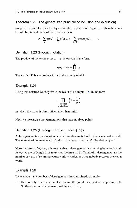
Definition 1.25 (Derangement sequence {dr})
A derangement is a permutation in which no element is fixed – that is mapped to itself.The number of derangements of r distinct objects is written dr. We define d0 = 1.
Note: in terms of cycles, this means that a derangement has no singleton cycles, allits cycles are of length 2 or more (see Lemma 4.16). Think of a derangement as thenumber of ways of returning coursework to students so that nobody receives their ownwork.
Example 1.26
We can count the number of derangements in some simple examples:
(i) there is only 1 permutation of {1} – and the (single) element is mapped to itself.So there are no derangements and hence d1 = 0;
12 1. What Is Enumeration?
(ii) there are 2 permutations of {1,2}: (1)(2) and (12). The last permutation has nofixed elements. Hence d2 = 1;
(iii) there are 6 permutations of {1,2,3}:
(1)(2)(3), (12)(3), (13)(2), (23)(1), (123) and (132).
The last 2 permutations are the only permutations that have no fixed elements andso d3 = 2.
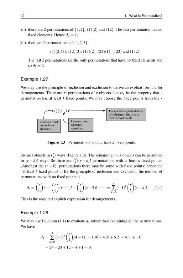
Example 1.27
We may use the principle of inclusion and exclusion to derive an explicit formula forderangements. There are r! permutations of r objects. Let αk be the property that apermutation has at least k fixed points. We may choose the fixed points from the r
Figure 1.3 Permutations with at least k fixed points.
distinct objects in(r
k
)ways (Figure 1.3). The remaining r−k objects can be permuted
in (r − k)! ways. So there are(r
k
)(r − k)! permutations with at least k fixed points.
(Amongst the (r− k)! permutations there may be some with fixed points: hence the“at least k fixed points”.) By the principle of inclusion and exclusion, the number ofpermutations with no fixed points is
dr =(
r0
)r!−
(r1
)(r−1)!+
(r2
)(r−2)!−·· · =
r
∑k=0
(−1)k(
rk
)(r− k)!. (1.1)
This is the required explicit expression for derangements.
Example 1.28
We may use Equation (1.1) to evaluate d4 rather than examining all the permutations.We have
d4 =4
∑k=0
(−1)k(
4k
)(4− k)! = 1.4!−4.3!+6.2!−4.1!+1.0!
= 24−24+12−4+1 = 9.
1.4 The Principle of Exhaustion 13
1.3.1 Exercises
Exercise 1.7
Find the number of integers less than 6,300 that are divisible by none of 3, 4and 5.
Exercise 1.8
How many permutations of {1,2,3,4} are there in which:
(i) 2 is not a fixed point;
(ii) 2 and 4 are not fixed points?
Exercise 1.9
A positive integer r is the product of the square of a prime and another prime,r = p2
1 p2. How many positive integers less than r are relatively prime to it?
Exercise 1.10
Prove that for any real number x, [x]+[x+ 1
2
]= [2x].
1.4 The Principle of Exhaustion
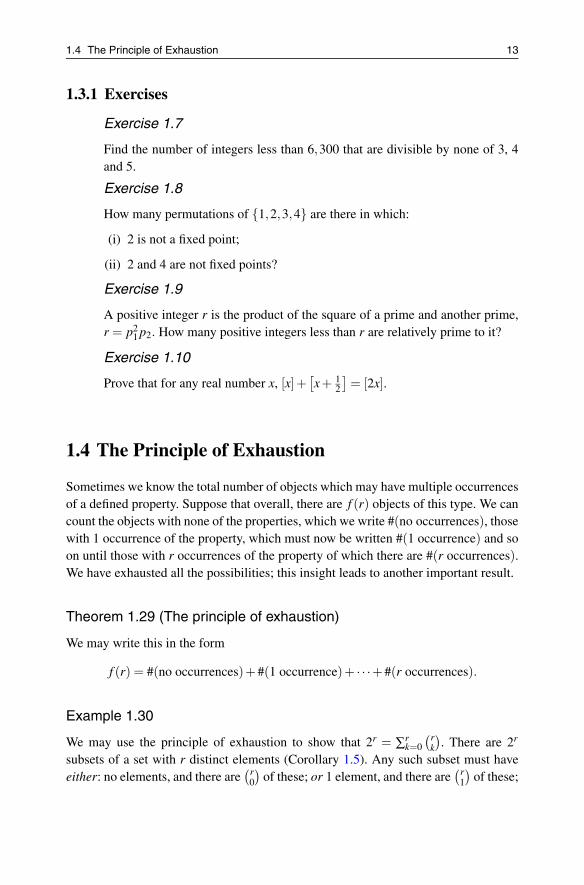
Sometimes we know the total number of objects which may have multiple occurrencesof a defined property. Suppose that overall, there are f (r) objects of this type. We cancount the objects with none of the properties, which we write #(no occurrences), thosewith 1 occurrence of the property, which must now be written #(1 occurrence) and soon until those with r occurrences of the property of which there are #(r occurrences).We have exhausted all the possibilities; this insight leads to another important result.
Theorem 1.29 (The principle of exhaustion)
We may write this in the form
f (r) = #(no occurrences)+#(1 occurrence)+ · · ·+#(r occurrences).
Example 1.30
We may use the principle of exhaustion to show that 2r = ∑rk=0
(rk
). There are 2r
subsets of a set with r distinct elements (Corollary 1.5). Any such subset must haveeither: no elements, and there are
(r0
)of these; or 1 element, and there are
(r1
)of these;

14 1. What Is Enumeration?
and so on until the subset has r elements, and there are(r
r
)of these. So by the principle
of exhaustion:
2r =r
∑k=0
(rk
)
as required.
Example 1.31
Another use of the principle of exhaustion is to prove a result concerning derangementnumbers. The number of permutations of r distinct objects is r!. We can construct andcount the permutations with a given number of fixed points. Any permutation haseither no fixed points, or 1 fixed point, . . ., or k fixed points (Figure 1.4).
Figure 1.4 Permutations with precisely k fixed points.
By the principle of exhaustion, we must have
r! =(
r0
)dr +
(r1
)dr−1 + · · ·+
(rr
)d0 =
r
∑k=0
(rk
)dr−k (1.2)
and this is the expression sought.
1.4.1 Exercises
Exercise 1.11
Use the principle of exhaustion to prove that(r+l
k
)= ∑k
m=0
( rm
)( lk−m
).
(Hint: r + l → ◦ ◦ · · ·◦︸ ︷︷ ︸r objects
◦ ◦ · · ·◦︸ ︷︷ ︸l objects
.)
Exercise 1.12
Suppose we want to count the permutations that have no 2-cycles, a general-ization of derangements. In the permutations of r objects we say there are br
permutations with no 2-cycles (b for bicycles!). We define b0 = 1.
1.4 The Principle of Exhaustion 15
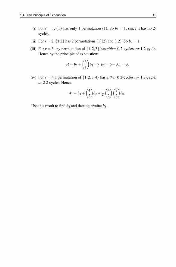
(i) For r = 1, {1} has only 1 permutation (1). So b1 = 1, since it has no 2-cycles.
(ii) For r = 2, {1 2} has 2 permutations (1)(2) and (12). So b2 = 1.
(iii) For r = 3 any permutation of {1,2,3} has either 0 2-cycles, or 1 2-cycle.Hence by the principle of exhaustion:
3! = b3 +(
31
)b1 ⇒ b3 = 6−3.1 = 3.
(iv) For r = 4 a permutation of {1,2,3,4} has either 0 2-cycles, or 1 2-cycle,or 2 2-cycles. Hence
4! = b4 +(
42
)b2 + 1
2!
(42
)(22
)b0.
Use this result to find b4 and then determine b5.


2Generating Functions Count
2.1 Counting – from Polynomials to Power Series
Consider the outcomes when a pair of dice are thrown and our interest is the sum ofthe numbers showing. One way to model the situation is by means of a grid in whicheach point (whose coordinates are non-negative integers 1 � x,y � 6) represents oneoutcome. In the grid below, the corresponding sum is shown alongside some of theresulting points:
Figure 2.1 Sum of two dice.
The problem with this model is that it does not help us to portray 3 dice, 4 diceor even more dice – the geometric insights become first difficult and then impossible.
A. Camina, B. Lewis, An Introduction to Enumeration,Springer Undergraduate Mathematics Series,DOI 10.1007/978-0-85729-600-9 2, © Springer-Verlag London Limited 2011
17

18 2. Generating Functions Count
We need to change our model. We may represent the first die by a polynomial
z+ z2 + z3 + z4 + z5 + z6.
The symbol z here is called an indeterminate which means that it is not a variablethat takes on values – its only role is to keep track of aspects of an enumeration. Itmay be replaced by X , by y or by any convenient symbol. In this instance it holds twoitems of information:
– the powers of z keep track of the different faces of the dice;
– the coefficients of the powers of z show the number of occurrences of each face.
The second die is represented by the same polynomial and the outcome of throw-ing two dice is represented – quite naturally – by
(z+ z2 + z3 + z4 + z5 + z6
)(z+ z2 + z3 + z4 + z5 + z6
).
By expanding this
z2 +2z3 +3z4 +4z5 +5z6 +6z7 +5z8 +4z9 +3z10 +2z11 + z12
we find that there is one way of obtaining a score of 2; there are two ways of gettinga score of 3; three ways of getting a score of 4 and so on. But – and this is the crucialadvantage of this algebraic model – the same method may be employed to find thenumber of ways that a particular score may be obtained with any number of dice. Itis important to ask why this works. We can obtain a score of 9 by getting the combi-nations (3,6), (6,3), (4,5) and (5,4). This is precisely the same as how many wayswe can get z9 when multiplying out the product above. So the coefficients enumer-ate. This is an important idea that we use time and time again. We formulate this inSubsection 5.4.2 as Theorem 5.17.
This ingenious idea of a polynomial counting things is the fundamental idea be-hind generating functions. Very often we will write down the generating function of anenumerative example in a form that needs to be “expanded”. There are two powerfultools that enable us to do this.
Theorem 2.1 (Binomial Theorem)
For a given integer r
(1+ z)r =
⎧⎪⎪⎪⎪⎨⎪⎪⎪⎪⎩
∑k�0
(rk
)zk if r > 0;
1 if r = 0;
∑k�0
(−1)k((−r+k−1
k
))zk if r < 0.
.

2.1 Counting – from Polynomials to Power Series 19
Moreover, the Binomial coefficients involved are given by the explicit form(
rk
)=
r(r−1) · · ·(r− k +1)k!
=r!
k!(r− k)!.
Convention: the sum ∑rk=0
(rk
)zk may be written ∑k�0
(rk
)zk in which the summation
index k takes the values k = 0 to k = ∞. As soon as k > r the Binomial coefficients arezero. This convention leads to concise ways of writing and dealing with such sums.Convergence: the first form of the sum is a finite sum because
(rk
)= 0 if k > r. It is
therefore valid for all values of z. This second form is valid for all values of z except−1, since 00 is undefined. The third form is a non-terminating expression (so it is aninfinite expansion); it is only valid when |z| < 1.
Example 2.2
The Binomial Theorem makes it easy to expand powers of expressions. For example:
(i)
(2+3z)7 = 27(
1+3z2
)7
= 27 ∑r�0
(7r
)(3z2
)r
= 27 +27(
71
)3z2
+27(
72
)32z2
22 + · · ·+27(
77
)37z7
27
= 128+1344z+6048z2 + · · ·+2187z7;
(ii)
(2+3z)−7 = 2−7(
1+3z2
)−7
= 2−7 ∑r�0
(7+ r−1
r
)(3z2
)r
= 2−7 +2−7 (71
) 3z2
+2−7 (82
) 32z2
22 + · · ·
=1
128+
21256
z+63128
z2 + · · · .
This expansion is valid only when∣∣ 3z
2
∣∣ < 1 that is, when |z| < 23 .
Theorem 2.3 (The sum of a geometric progression (GP))
In the finite case, we have:
1+ z+ z2 + · · ·+ zn =n
∑r=0
zr =
{1−zn+1
1−z if z �= 1;
n+1 otherwise.(2.1)

20 2. Generating Functions Count
If |z| < 1 we can evaluate the infinite sum:
1+ z+ z2 + · · · = ∑r�0
zr =1
1− z. (2.2)
We return to generating functions and the way in which these results may be ex-ploited.
Example 2.4
We explore the number of ways there are to obtain a score of 12 with the throw offive dice. Simple: it is the coefficient of z12 in the product of five polynomials, each ofwhich enumerates the outcomes of a single die:
(z+ z2 + z3 + z4 + z5 + z6
)5.
Now we proceed to expand and simplify this using Theorem 2.1 and Equation (2.1).We have,
(z+ z2 + z3 + z4 + z5 + z6
)5= z5
(1+ z+ z2 + z3 + z4 + z5
)5
=z5
(1− z6
)5
(1− z)5
= z5(
1− z6)5
(1− z)−5
=(
z5 −5z11 + · · ·− z35)
∑r�0
(r +4
4
)zr.
So the coefficient of z12 is just
(7+4
4
)−5
(1+4
4
)= 330−25 = 305.
There are 305 ways to obtain a score of 12 when five dice are thrown.
Example 2.5
A generous father wishes to divide £20 between his daughters Emma and Pippa, andson Leon, so that they each receive at least £5, nobody receives more than £10, andEmma gets an even amount. How many ways are there of doing this? What we seekare the non-negative, integer solutions to the equation e + p + l = 20 subject to the

2.1 Counting – from Polynomials to Power Series 21
conditions that 5 � e, p, l � 10 and e is even. Viewed in this way, we may associate apolynomial with each recipient:
z5 + z6 + z7 + z8 + z9 + z10
for Pippa and Leon, together with
z6 + z8 + z10
for Emma. Each of these enumerates the amounts they might receive. The answer toour problem is the coefficient of z20 in the product(
z6 + z8 + z10)(
z5 + z6 + z7 + z8 + z9 + z10)2
Once again, thanks to Theorem 2.1 and Equation (2.1) it is easier to find than it looks.The expression may be re-written, and then manipulated
(z6 + z8 + z10
)(z5 + z6 + z7 + z8 + z9 + z10
)2= z16 (
1+ z2 + z4)(1− z6
1− z
)2
= z16
(1+ z2 + z4
)(1−2z6 + z12
)(1− z)2
=(
z16 + z18 + · · ·+ z32)
∑r�0
(r +1
1
)zr.
The required coefficient of z20 is now easy to pick out. It is(
51
)+
(31
)+
(11
)= 5+3+1 = 9.
The expressions we have used to help us count in Examples 2.4 and 2.5 were madeup from polynomials. This is because the terms in which we were interested onlyhad a finite number of possibilities. In Example 2.4 the only possible scores are5,6,7, . . . ,28,29,30. They make up a finite sequence {1,2, . . . ,30}.
Many enumerations are not finite and result in a sequence that does not terminate:for example the number of subsets of a set with r elements. In dealing with an infi-nite sequence, we need infinite expressions. This leads us to the idea of a generatingfunction.
Definition 2.6 (Generating function)
Given any sequence {ur} = {u0,u1,u2, · · ·}, a generating function U(z) for the se-quence is an expression (called a power series in the infinite case and a polynomial inthe finite case) in which,
U(z) = u0 +u1z+u2z2 + · · · = ∑r�0
urzr.
22 2. Generating Functions Count
This definition has two parts:
(i) the power series (or polynomial) on the right, each of whose coefficients is aterm of the sequence placed against a power of the indeterminate z that matchesits position in the sequence;
(ii) the function U(z) that explicitly represents the power series, or polynomial fol-lowing some re-arrangement.
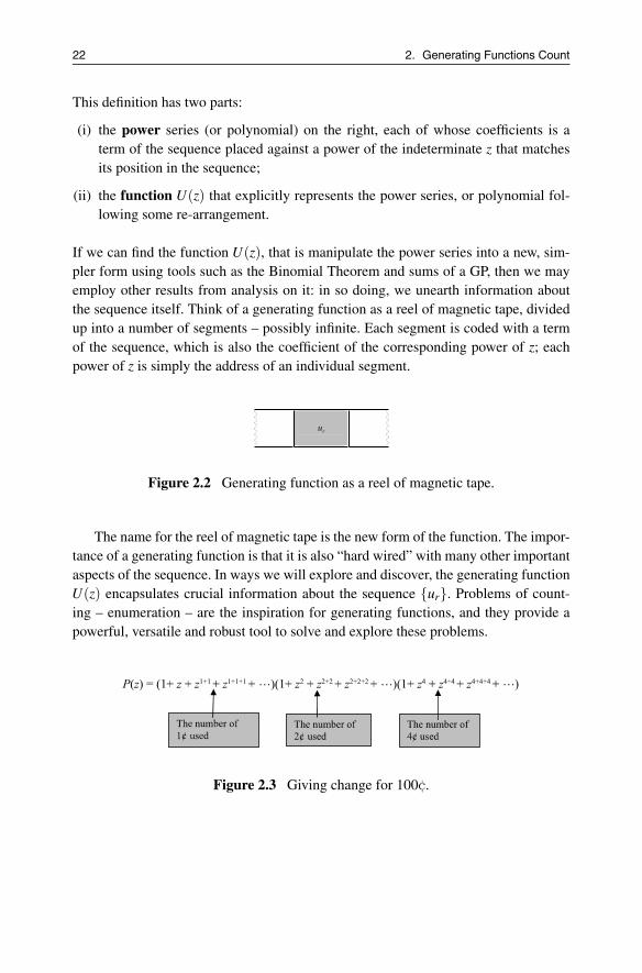
If we can find the function U(z), that is manipulate the power series into a new, sim-pler form using tools such as the Binomial Theorem and sums of a GP, then we mayemploy other results from analysis on it: in so doing, we unearth information aboutthe sequence itself. Think of a generating function as a reel of magnetic tape, dividedup into a number of segments – possibly infinite. Each segment is coded with a termof the sequence, which is also the coefficient of the corresponding power of z; eachpower of z is simply the address of an individual segment.
Figure 2.2 Generating function as a reel of magnetic tape.
The name for the reel of magnetic tape is the new form of the function. The impor-tance of a generating function is that it is also “hard wired” with many other importantaspects of the sequence. In ways we will explore and discover, the generating functionU(z) encapsulates crucial information about the sequence {ur}. Problems of count-ing – enumeration – are the inspiration for generating functions, and they provide apowerful, versatile and robust tool to solve and explore these problems.
Figure 2.3 Giving change for 100¢.

2.1 Counting – from Polynomials to Power Series 23
Example 2.7
Imagine a country in which there are only three coins: a 1¢ coin, a 2¢ coin and a 4¢coin – this is a very mathematical country. We determine the generating function forthe enumeration of the number of ways that change may be given for 100¢. We needto solve the equation r +2s+4t = 100 for non-negative integers r, s and t. We do thisby finding the coefficient of z100 in a generating function (Figure 2.3).
We could, of course, multiply out initial terms of each bracket, and with someperseverance we might eventually find the coefficient of z100. But now we exploit thegenerating function by concentrating on the right-hand side – seeking an easier formfor it.
We start by writing the generating function in the form
P(z) = (1+ z+ z2 + z3 + · · ·)(1+ z2 + z4 + z6 + · · ·)(1+ z4 + z8 + z12 + · · ·).
And now for the decisive step: each of the bracketed expressions is a GP, so when|z| < 1, we have
P(z) =1
(1− z)(1− z2)(1− z4).
Now we use partial fractions and find that
P(z) =1
8(1− z)3 +1
4(1− z)2 +9
32(1− z)+
116(1+ z)2 +
532(1+ z)
+1+ z
8(1+ z2).
We may expand each term on the right using the Binomial Theorem; the coefficient ofz100 is simply:
18
(1022
)+
14
(102
1
)+
932
+(−1)100
16
(101
1
)+
5(−1)100
32+
(−1)50
8= 676.
That’s the power of generating functions – it even provides the answer for any amountof money, but we’ll pick that up again later. This example made use of another power-ful tool: partial fractions. This is a technique that comes into its own with generatingfunctions.
2.1.1 Exercises
Exercise 2.1
What is the generating function for the score obtained when ten dice arethrown? Use this to find the number of ways that a score of 25 may be ob-tained. (Leave your answer in binomial form.)

24 2. Generating Functions Count
Exercise 2.2
The equation x + 2y + 4z = 100 determines a plane in three-dimensional Eu-clidean space. How many non-negative lattice points (a lattice point is a pointeach of whose coordinates is an integer) lie on this plane?
Exercise 2.3
How many ways are there to give change for £2 if the coinage is 1p and 3p.
Exercise 2.4
Show that the distinct divisors of p21 p3
2 (where p1 and p2 are primes) are gen-erated by the expression
(1+ p1 + p2
1
)(1+ p2 + p2
2 + p32
).
Deduce that an arbitrary positive integer r whose prime factorization is
r = pa11 pa2
2 · · · pakk
hask
∏m=1
(1+am)
distinct divisors.
2.2 Recurrence Relations and Enumeration
When we examine a particular enumeration, we frequently resort to breaking downone of its configurations into smaller parts, so that we can understand how it is madeup. Mathematically this may be expressed as a relation between configurations ofdifferent “sizes”. Such an expression is called a recurrence relation and they comein all sorts of varieties.
Definition 2.8 (Recurrence relation (informal))
The recurrence relation satisfied by a sequence is a recipe that uses initial terms as theingredients for subsequent terms. It is usually “seeded” by some initial values.
Although recurrences are often the starting point in the analysis of an enumeration,deriving a recurrence relation is by no means easy or obvious. We have a numberof tools in the enumerative toolbox that help, such as the principle of exhaustion,that were set out in Chapter 1. This section concentrates on this crucial first step –constructing a recurrence by analyzing how the objects of different sizes fit together.

2.2 Recurrence Relations and Enumeration 25
Example 2.9
We start by finding a recurrence satisfied by the number of denary strings of length r,see Definition 1.3, in which between them the digits {3,6,9} occur an even numberof times. The strategy is to construct an object of “size” r +1 from those of “size” r.
Figure 2.4 Denary strings.
Call the number of legal strings of length r, nr. A legal string of length r + 1 hasone of the forms NLa or NNLb where:
– NL is a legal string of length r so a ∈ {0,1,2,4,5,7,8};
– NNL is not a legal string of length r so b ∈ {3,6,9}.
It follows that
nr+1 = #(a).#(NL)+#(b).#(NNL) = 7#(NL)+3#(NNL)
= 3 [#(NL)+#(NNL)]+4#(NL) .
The total number of strings of length r is 10r and so
nr+1 = 3.10r +4#(NL) = 3.10r +4nr.
This is the required recurrence. Once we know one initial value we can use therecurrence to creep forwards, finding successive terms of the sequence, one at a time.
Example 2.10
We have n1 = 7 so that n2 = 3.101 + 4n1 = 58 and n3 = 3.102 + 4n2 = 532; we maycontinue this as far as we please.
Here is another example, this time with a geometric flavour – and with a sequenceas answer that turns out to be very important.

26 2. Generating Functions Count
Example 2.11
A car park consists of a row of r spaces; a motorbike (m) takes one space, a car (c)two.
Figure 2.5 Parking cars and motorbikes.
We seek the number of ways there are of filling the spaces. Call the number of waysof filling r spaces, pr. The strategy is to use the principle of exhaustion on the finalparking space. Either there is a car or a motorbike in the final space and so the formof any parking arrangement has one of the two possibilities Pr−1m or Pr−2c where
– Pr−1 is a parking arrangement of r−1 places, and m is a motorbike;
– Pr−2 is a parking arrangement of r−2 places and c is a car.
Hence,
#(Pr) = #(m) .#(Pr−1)+#(c) .#(Pr−2)
which means that the required recurrence is
pr = pr−1 + pr−2.
We easily find that p1 = 1 and p2 = 2, so then p3 = 3, p4 = 5, p5 = 8, and the sequenceproceeds, each term being the sum of the two preceding terms.
The terms of this sequence are called Fibonacci numbers and we meet them onmany occasions. We define p0 = 1 as this is the only value consistent with the recur-rence relation.The sequence {pr} is not the Fibonacci sequence, which we denote by{Fr}. In fact we have
pr = Fr+1
and so the sequence {pr} does consist of Fibonacci numbers, but they are displacedby one step.
2.2 Recurrence Relations and Enumeration 27
Example 2.12
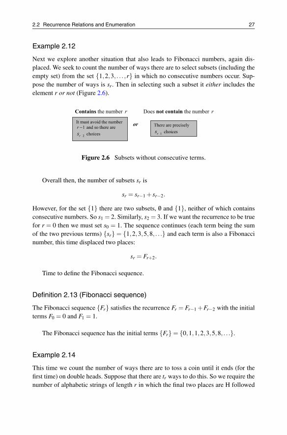
Next we explore another situation that also leads to Fibonacci numbers, again dis-placed. We seek to count the number of ways there are to select subsets (including theempty set) from the set {1,2,3, . . . ,r} in which no consecutive numbers occur. Sup-pose the number of ways is sr. Then in selecting such a subset it either includes theelement r or not (Figure 2.6).
Figure 2.6 Subsets without consecutive terms.
Overall then, the number of subsets sr is
sr = sr−1 + sr−2.
However, for the set {1} there are two subsets, /0 and {1}, neither of which containsconsecutive numbers. So s1 = 2. Similarly, s2 = 3. If we want the recurrence to be truefor r = 0 then we must set s0 = 1. The sequence continues (each term being the sumof the two previous terms) {sr} = {1,2,3,5,8, . . .} and each term is also a Fibonaccinumber, this time displaced two places:
sr = Fr+2.
Time to define the Fibonacci sequence.
Definition 2.13 (Fibonacci sequence)
The Fibonacci sequence {Fr} satisfies the recurrence Fr = Fr−1 +Fr−2 with the initialterms F0 = 0 and F1 = 1.
The Fibonacci sequence has the initial terms {Fr} = {0,1,1,2,3,5,8, . . .}.
Example 2.14
This time we count the number of ways there are to toss a coin until it ends (for thefirst time) on double heads. Suppose that there are tr ways to do this. So we require thenumber of alphabetic strings of length r in which the final two places are H followed

28 2. Generating Functions Count
by another H, preceded by a string of Hs and Ts in which the string “HH” does notoccur. Such a string starts either with a tail or a head (which is then followed by atail): Figure 2.7.
Figure 2.7 Alphabetic strings that end on HH.
Overall then, the number of strings tr is
tr = tr−1 + tr−2.
For one toss of a coin the outcomes are either T or H. So t1 = 0 since neither of theseends in a double head. Similarly, t2 = 1, t3 = 1 and hence
tr = Fr−1.
If we define F−1 = 1 (a value consistent with the Fibonacci recurrence relation) thenthis is true when r � 0.
The next example exploits Fibonacci numbers but results in another sequence ofimportance.
Example 2.15
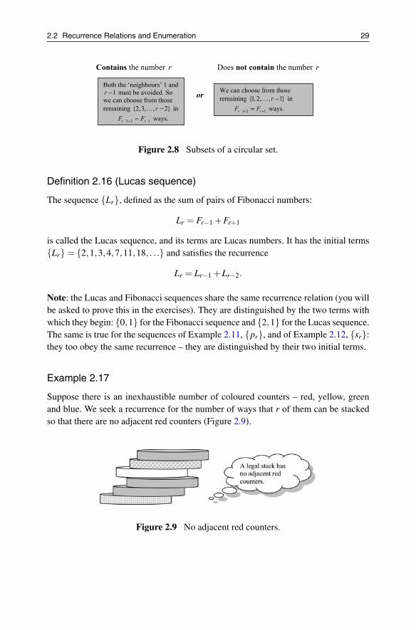
We count the number of ways we can select a subset from the circular set {1,2,3, . . . ,r}that does not contain consecutive numbers. (Circular here, means that we regard 1 andr as consecutive, and again, we include the empty set as an allowable subset choice.)Suppose the number of such selections is Lr. A selection either contains the elementr, or not (Figure 2.8).
From Example 2.12 we know the number of ways that subsets (without consecu-tive elements) may be chosen from a set of r elements is Fr+2. Overall then, we have
Lr = Fr−3+2 +Fr−1+2 = Fr−1 +Fr+1.
The sequence that appears here is a sibling sequence to the Fibonacci sequence.
2.2 Recurrence Relations and Enumeration 29
Figure 2.8 Subsets of a circular set.
Definition 2.16 (Lucas sequence)
The sequence {Lr}, defined as the sum of pairs of Fibonacci numbers:
Lr = Fr−1 +Fr+1
is called the Lucas sequence, and its terms are Lucas numbers. It has the initial terms{Lr} = {2,1,3,4,7,11,18, . . .} and satisfies the recurrence
Lr = Lr−1 +Lr−2.
Note: the Lucas and Fibonacci sequences share the same recurrence relation (you willbe asked to prove this in the exercises). They are distinguished by the two terms withwhich they begin: {0,1} for the Fibonacci sequence and {2,1} for the Lucas sequence.The same is true for the sequences of Example 2.11, {pr}, and of Example 2.12, {sr}:they too obey the same recurrence – they are distinguished by their two initial terms.
Example 2.17
Suppose there is an inexhaustible number of coloured counters – red, yellow, greenand blue. We seek a recurrence for the number of ways that r of them can be stackedso that there are no adjacent red counters (Figure 2.9).
Figure 2.9 No adjacent red counters.

30 2. Generating Functions Count
The enumerative strategy is to construct a stack of “size” r+1 from one of “size” r.Suppose that we denote the number of legal stacks by sr. In constructing sr+1 for r � 2we use the principle of exhaustion on the topmost counter; every legal stack either hasthe form SRc1 or SNRc2, where:
(i) SR is a legal stack (of size r) that ends with a red counter, so that c1 ∈ {Y,G,B};
(ii) SNR is a legal stack (of size r) that does not end with a red counter, so that c2 ∈{R,Y,G,B}.
It follows that,
sr+1 = 3#(SR)+4#(SNR)
= 3 [#(SR)+#(SNR)]+#(SNR) = 3sr +#(SNR) .
However #(SNR) = 3sr−1 since it can be made from a legal stack of size r−1 followedby a final counter that may be chosen from three pieces: {Y,G,B}. So
sr+1 = 3sr +3sr−1.
We note that s1 = 4, s2 = 15 = (4.4−1) so that s3 = 3.s2 +3.s1 = 57 and s4 = 3.57+3.15 = 216. Again, we can continue calculating as many terms of the sequence asdesired – though it does become very tedious.
Example 2.18
A geometric example: finding the number of regions created when r lines are drawnin the plane – no two of which are parallel, and no three of which are coincident(Figure 2.10).
Figure 2.10 Regions created by four lines.
2.2 Recurrence Relations and Enumeration 31
Suppose we denote the number of regions by Rr. The rth line meets each of the otherr−1 lines in a distinct point (because of the conditions) and these r−1 points of in-tersection divide the rth line into r sections. Each of these sections divides an existingregion into two regions, adding one new region.
So, when the rth line is drawn, the number of regions increases by r. We have therecurrence:
Rr = Rr−1 + r and R0 = 1.
We met the derangement sequence {dr} in Equation (1.2); there we showed that itsterms, called derangement numbers, satisfy a rather complicated recurrence relation:
r! =r
∑k=0
(rk
)dr−k.
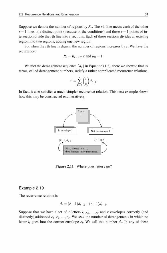
In fact, it also satisfies a much simpler recurrence relation. This next example showshow this may be constructed enumeratively.
Figure 2.11 Where does letter i go?
Example 2.19
The recurrence relation is
dr = (r−1)dr−2 +(r−1)dr−1.
Suppose that we have a set of r letters l1, l2, . . . , lr and r envelopes correctly (anddistinctly) addressed e1,e2, . . . ,er. We seek the number of derangements in which noletter li goes into the correct envelope ei. We call this number dr. In any of these

32 2. Generating Functions Count
derangements letter 1 must be placed in envelope i where 2 � i � r. Now we exhaustthe possibilities for letter i (see Figure 2.11):
– either letter i is in envelope 1
– or letter i is not in envelope 1.
Overall then, we have
dr = (r−1)dr−2 +(r−1)dr−1.
The importance of this new recurrence is its simplicity. It may also be deriveddirectly from the explicit formula (Equation 1.1, page 12) – see Exercise 2.8.
2.2.1 Exercises
Exercise 2.5
Let ar be the number of legal arithmetic “expressions” that are made up of ritems chosen from the operations {+,×,/} and the digits {0,1,2, . . . ,9}. Alegal arithmetic expression is one that can be evaluated: 2+3×5 is legal, as is57; while 8+×9 is not. Find a recurrence relation for ar.
Exercise 2.6
Find a recurrence for the number of binary strings, made up of r digits drawnfrom 0,1 which do not have consecutive 0s.
Exercise 2.7
Let ur be the number of ways that the natural number r may be written as asum of 1s and 2s, in which the order of the summands is counted. For example:u2 = 2 since 2 ≡ 2 = 1+1, while u3 = 3 since 3 ≡ 2+1 = 1+2 = 1+1+1.
Find a recurrence relation satisfied by the sequence ur.
Exercise 2.8
Given the explicit formula (Equation 1.1)
dr =r
∑k=0
(−1)k(
rk
)(r− k)!
prove that the derangement sequence satisfies the recurrence dr = rdr−1 +(−1)r. Then show that this recurrence leads to the recurrence of Example 2.19.
Exercise 2.9
Prove that the Lucas sequence satisfies the same recurrence as that for the Fi-bonacci sequence:
Lr = Lr−1 +Lr−2.
2.3 Sequence to Generating Function 33
2.3 Sequence to Generating Function
There are two routes to a generating function. The first starts with the sequence itself,and assumes that we know all of its terms.
2.3.1 Sequence to Generating Function
We start with a simple example of a sequence with known terms and seek to find itsgenerating function – that is, we want this as a function in an explicit form rather thanas a power series.
Example 2.20
We can easily find the generating function of the sequence {ur} = {1,1,1, . . .}. Thegenerating function is the power series
1+1z+1z2 + · · · = 1+ z+ z2 + · · · .
However, we note that if |z| < 1 this is a convergent geometric progression, so byEquation (2.2)
U(z) =1
1− z.
The function U(z) is the generating function for the sequence {ur}= {1,1,1, . . .}. Wemay use this generating function to find generating functions for other sequences.
Example 2.21
The generating function of the last example may be written like this
11− z
= 1+ z+ z2 + z3 + · · · .
If we differentiate both sides then we obtain:
1(1− z)2 = 1+2z+3z2 +4z3 + · · · .
(Term-by-term differentiation of a power series is valid when it is absolutely conver-gent; in this case when |z| < 1.) This new expression is simply another generatingfunction for another sequence: the function
1(1− z)2

34 2. Generating Functions Count
is the generating function for the sequence
{1,2,3, . . .} = {r +1}.
We can also integrate absolutely convergent power series to create another “newsequence for old”. Using operations like this we can build a library of sequences andtheir generating functions. There are other operations we can use as well.
Example 2.22
If we multiply the generating function of the last example by z we find that
z(1− z)2 = z+2z2 +3z3 +4z4 + · · · .
We may conclude that the sequence
{0,1,2,3, . . .} = {r}
has the generating functionz
(1− z)2 .
So our generating function library now consists of
Table 2.1 Generating function library.
We will build the library as the book progresses and it is summarized in Appendix A.
2.3.2 Recurrence to Generating Function
Most enumerations start with a recurrence relation that has been derived, rather thanthe enumerative sequence itself. Once we have such a recurrence relation for a se-quence of interest, we have seen that it can be used to find successive terms of the
2.3 Sequence to Generating Function 35
sequence. But there are much more powerful ways of exploiting the recurrence to findthis and other properties of the sequence – the route to these methods goes through agenerating function. So we turn to the problem of converting a recurrence into a gen-erating function. There is a standard way that we go about this task – and it follows arecipe with three steps.
Algorithm 2.23 (Recurrence to generating function – three-step recipe)
The three parts of the recipe to convert a recurrence into a generating function are:
(i) write out recurrence;
(ii) multiply through by zr and sum for valid r;
(iii) invoke generating and other library functions.
Example 2.24
We illustrate the recipe by converting the recurrence ur = 5ur−1−6ur−2 with the initialvalues u0 = 5 and u1 = 12 for the sequence {ur} into a generating function.
(i) The first step is ur = 5ur−1 −6ur−2.
(ii) The second step then becomes,
∑r�2
urzr = ∑r�2
5ur−1zr − ∑r�2
6ur−2zr. (2.3)
(Note that as there is a term r−2 in the recurrence, we take r � 2.)
(iii) The final step is where all the action takes place. The generating function we seekis, U(z) = ∑r�0 urzr which is almost the term on the left of Equation (2.3); so wewrite,
U(z) = u0 +u1z+ ∑r�2
urzr = 5+12z+ ∑r�2
urzr
⇒ ∑r�2
urzr = U(z)−5−12z.
Now for the first term on the right of Equation (2.3). We have,
∑r�2
5ur−1zr = 5z ∑r�2
ur−1zr−1 = 5z
(∑r�1
ur−1zr−1 −u0
)
= 5zU(z)−25z.

36 2. Generating Functions Count
The final term is now easy
∑r�2
6ur−2zr = 6z2 ∑r�2
ur−2zr−2 = 6z2U(z).
We put each of these results into Equation (2.3):
U(z)−5−12z = 5zU(z)−25z−6z2U(z)
and then solve this for U(z). We find that
U(z) =5−13z
1−5z+6z2 .
We have quickly passed over a very important idea which we now make explicit. Thisimportant result, whose proof is immediate, should become second nature.
Theorem 2.25 (Re-indexing a sum)
We haveU(z) = ∑
r�0urz
r = ∑r�1
ur−1zr−1 = ∑r�2
ur−2zr−2 . . .
Most of the recurrences that we encountered in the last section can be convertedinto generating functions by the three-step recipe. A notable exception is the derange-ment sequence – we must wait for Chapter 7 for that.
Example 2.26
The recurrence relation satisfied by the Fibonacci sequence {Fr} is Fr = Fr−1 + Fr−2
with the initial values F0 = 0 and F1 = 1. Applying the three-step recipe gives:
(i) The recurrence is Fr = Fr−1 +Fr−2.
(ii) Then we sum on the index r with corresponding powers of z:
∑r�2
Frzr = ∑
r�2
Fr−1zr + ∑r�2
Fr−2zr.
(iii) Finally
∑r�0
Frzr −F0 −F1z = z
(∑r�0
Fr−1zr−1 −F0
)+ z2 ∑
r�0Frz
r.

2.3 Sequence to Generating Function 37
Using the initial values and denoting the generating function by F(z), we have
F(z)−0− z = z(F(z)−0)+ z2F(z)
and we can solve this for the required generating function F(z):
F(z) = ∑r�0
Frzr =
z1− z− z2 .
Working in the same way with the recurrence Lr = Lr−1 + Lr−2 with the initialvalues L0 = 2 and L1 = 1 of the Lucas sequence and denoting the generating functionby L(z), we find that
L(z) = ∑r�0
Lrzr =
2− z1− z− z2 .
Note: the generating functions of these two sequences have the same denominator;also note that they obey the same recurrence. We will explore this later.
Example 2.27
We will convert the recurrence of Example 2.18 into a generating function.
(i) The recurrence is:Rr = Rr−1 + r and R0 = 1.
(ii) The next step is
∑r�1
Rrzr = ∑
r�1
Rr−1zr + ∑r�1
rzr.
(iii) In this final step we draw on our library of generating functions for the last termon the right. We can also re-write the other terms. We then have:
∑r�0
Rrzr −R0 = z ∑
r�0
Rrzr +
z(1− z)2 .
If we let the generating function be R(z) then we have
R(z)−1 = zR(z)+z
(1− z)2
and hence
R(z) =1− z+ z2
(1− z)3 .

38 2. Generating Functions Count
2.3.3 Exercises
Exercise 2.10
Find generating functions for the sequences
(i) {vr} = {1,−1,1,−1, . . .};
(ii) {ur} = {1,−2,3,−4, . . .};
(iii) {or} = {1,0,3,0,5,0, . . .}.
Exercise 2.11
Integrate the expression 11−z = 1 + z + z2 + · · · and determine the constant of
integration by assigning the value z = 0. What is the generating function forthe Reciprocal sequence, {0,1, 1
2 , 13 , 1
4 , . . .}?
Exercise 2.12
A sequence {ur} obeys the recurrence relation, ur = ur−1 +2ur−2 with u0 = 4and u1 = 5. Find the generating function for the sequence.
Exercise 2.13
The sequence {ar} satisfies the recurrence relation ar = 2ar−1 + 15ar−2 witha0 = 4 and a1 = 4. Find the generating function of the sequence {ar}.
Exercise 2.14
Use the recurrence and the initial terms of the Lucas sequence {Lr} to confirmthat its generating function is as given in Example 2.26.
2.4 Miscellaneous Exercises
Exercise 2.15
Find a generating function for the number of strings of length r made up fromthe digits {0,1,2,3} in which there is never a 3 anywhere to the right of 0.
Exercise 2.16
We define the matrix M as the 2×2 array:
M =(
0 11 1
).
The powers of this matrix have a number of surprising connections with Fi-bonacci and Lucas numbers.

2.4 Miscellaneous Exercises 39
(i) Show that
Mr =(
Fr−1 Fr
Fr Fr+1
).
(ii) show that the trace of Mr is given by tr(Mr) = Lr;
(iii) by considering the determinant of Mr prove Cassini’s identity
Fr−1Fr+1 −F2r = (−1)r.
Exercise 2.17
Find a generating function for the number of non-negative integer solutions tothe equation a+2b = r for each positive integer r.
Exercise 2.18
A mathematics examination consists of six modules each with m marks. Showthat the number of ways a candidate may score precisely 3m marks (the “passmark”) overall is (
3m+55
)−6
(2m+4
5
)+15
(m+3
5
).
Exercise 2.19
In this exercise we investigate the number of ways pr in which a positive integermay be written as the ordered sums of the summands {1,2,3}. For example:one can only be written as 1 so p1 = 1; however two may be written as 2 = 2 =1+1 and hence p2 = 2. Three has four ways of being written, 3 = 3 = 2+1 =1+2 = 1+1+1 and hence p3 = 4. Find a recurrence relation for the terms ofthe sequence {pr}.
Exercise 2.20
You are given two tiles – one a unit square, and the other a rectangle madeup from two unit squares. The rectangle can be laid vertically or horizontally.We denote the number of ways of tiling a 2 × r rectangle by fr. Show thatfr = 2 fr−1 + 3 fr−2 and hence find a generating function for the number oftilings.


3Working with Generating Functions
We have explored a range of enumerative problems by finding a recurrence relationthat the corresponding count satisfies. This means that once we have some initialterms, we can progressively calculate more. We have also developed a way to con-vert some recurrence relations into a generating function. If we can manipulate thegenerating function and then expand it as a power series that enables us to give ex-plicit expressions for the count by reading off the coefficient of a particular power ofthe indeterminate used. This last step is the focus of this chapter. Along the way wealso explore the different recurrences satisfied by the corresponding sequence.
3.1 Expanding Generating Functions
We start with a generating function of a particularly form.
Example 3.1 (Generating functions with a simple denominator)
We start with the sequence that counted the number of regions in the plane created byintersecting lines – Example 2.18. The generating function is
R(z) = ∑r�0
Rrzr =
1− z+ z2
(1− z)3 .
A. Camina, B. Lewis, An Introduction to Enumeration,Springer Undergraduate Mathematics Series,DOI 10.1007/978-0-85729-600-9 3, © Springer-Verlag London Limited 2011
41

42 3. Working with Generating Functions
But we can expand the denominator by the Binomial Theorem and then
∑r�0
Rrzr =
(1− z+ z2)(1− z)−3 =
(1− z+ z2) ∑
r�0
(r +2
2
)zr.
In effect this gives us an explicit form for the number of regions – a major break-through. All we need to do is to write out (as far as we please) the power series on theright:
(1− z+ z2)((
22
)+
(32
)z+
(42
)z2 + · · ·
)
=(
22
)+
(32
)z+
(42
)z2 +
(52
)z3 + · · ·
−(
22
)z−
(32
)z2 −
(42
)z3 + · · ·
+(
22
)z2 +
(32
)z3 +
(42
)z4 + · · ·
= 1+(3−1)z+(6−3+1)z2 +(10−6+3)z3 + · · · .
It is easy to see how the general term is formed from Binomial coefficients:
Rr =(
r +22
)−
(r +1
2
)+
(r2
)= 1
2
(r2 + r +2
).
We often refer to this final part as “comparing coefficients of zr on either side”.This selects the rth term of the enumerative sequence on the left and an explicit expres-sion for it on the right. This is one of the principal reasons why generating functionsare so useful.
Example 3.2
We expand as a power series the function given by (1+ z)/(1−3z)2.
∑r�0
arzr =
1+ z(1−3z)2 = (1+ z)(1−3z)−2 ;
then we may expand the final term by the Binomial Theorem which gives
= (1+ z) ∑r�0
(r +1)3rzr.
This function generates the sequence {ar} and when we compare coefficients of zr oneither side we have
ar = (r +1)3r + r3r−1 = (4r +3)3r−1
which is true for r � 0.

3.1 Expanding Generating Functions 43
These two examples show that a generating function whose denominator is apower of a linear expression can certainly be expanded – in a particularly simple way.Unfortunately, not all generating functions are of this form.
Example 3.3 (Generating functions with a quadratic denominator)
Suppose we are given the generating function (whose denominator is quadratic) forthe sequence {ur}
∑r≥0
urzr =
5−13z1−5z+6z2 .
We notice that the denominator factorizes (over the integers) so that
∑r≥0
urzr =
5−13z(1−2z)(1−3z)
.
Once more partial fractions come to our aid
∑r≥0
urzr =
31−2z
+2
1−3z.
If we expand each term by the Binomial Theorem, we have
∑r≥0
urzr = 3 ∑
r≥02rzr +2 ∑
r≥03rzr
and comparing coefficients of zr gives the explicit form
ur = 3.2r +2.3r.
But what if the denominator does not factorize? We now investigate such a gener-ating function – that for the Lucas sequence (Exercise 2.14).
Example 3.4
We start with the generating function of the Lucas sequence {Lr} which is
L(z) = ∑r�0
Lrzr =
2− z1− z− z2 .
The denominator cannot be factorized (over the integers) but we can write
1− z− z2 = (1−φ1z)(1−φ2z) (3.1)

44 3. Working with Generating Functions
and comparing coefficients of zr (for r = 1,2) we must have φ1 + φ2 = 1 and φ1φ2 =−1. Using these relations we may write the generating function in the form
L(z) = ∑r�0
Lrzr =
2− z(1−φ1z)(1−φ2z)
.
Then using standard partial fraction techniques wefind that
L(z) = ∑r�0
Lrzr =
11−φ1z
+1
1−φ2z.
Now we can expand each term on the right
∑r�0
Lrzr =
(1+φ1z+φ2
1z2 + · · ·)+
(1+φ2z+φ2
2z2 + · · ·)
= ∑r�0
(φr1 +φr
2)zr
and so on comparing powers of zr we have the formula
Lr = φr1 +φr
2.
We can now make this explicit, by solving the two relations that come from Equa-tion (3.1). These reduce to a quadratic whose roots are φ1 = 1+
√5
2 and φ2 = 1−√
52 . We
have proved the theorem that follows.
Theorem 3.5 (Binet’s formula for the Lucas sequence)
Each term of the sequence is given by an expression called Binet’s formula for theLucas numbers:
Lr = φr1 +φr
2 =
(1+
√5)r
+(
1−√
5)r
2r .
The Lucas sequence {Lr} has a celebrity sibling, the Fibonacci sequence {Fr}. Theyshare many properties. We derive a corresponding Binet formula for them.
Example 3.6
The generating function for the Fibonacci sequence may be factorized (as in the lastexample)
∑r≥0
Frzr =
z(1−φ1z)(1−φ2z)
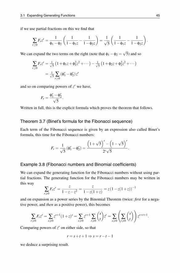
3.1 Expanding Generating Functions 45
if we use partial fractions on this we find that
∑r≥0
Frzr =
1φ1 −φ2
(1
1−φ1z− 1
1−φ2z
)=
1√5
(1
1−φ1z− 1
1−φ2z
).
We can expand the two terms on the right (note that φ1 −φ2 =√
5) and so
∑r≥0
Frzr = 1√
5
(1+φ1z+φ2
1z2 + · · ·)− 1√
5
(1+φ2z+φ2
2z2 + · · ·)
= 1√5 ∑
r≥0
(φr1 −φr
2)zr
and so on comparing powers of zr we have,
Fr =φr
1 −φr2√
5.
Written in full, this is the explicit formula which proves the theorem that follows.
Theorem 3.7 (Binet’s formula for the Fibonacci sequence)
Each term of the Fibonacci sequence is given by an expression also called Binet’sformula, this time for the Fibonacci numbers:
Fr =1√5
(φr1 −φr
2) =
(1+
√5)r
−(
1−√
5)r
2r√
5.
Example 3.8 (Fibonacci numbers and Binomial coefficients)
We can expand the generating function for the Fibonacci numbers without using par-tial fractions. The generating function for the Fibonacci numbers may be written inthis way
∑r�0
Frzr =
z1− z− z2 =
z1− z(1+ z)
= z(1− z(1+ z))−1
and on expansion as a power series by the Binomial Theorem (twice: first for a nega-tive power, and then as a positive power), this becomes
∑r�0
Frzr = ∑
s�0
zs+1(1+ z)s = ∑s�0
zs+1 ∑t�0
(st
)zt = ∑
s�0
(∑t�0
(st
))zs+t+1.
Comparing powers of zr on either side, so that
r = s+ t +1 ⇒ s = r− t −1
we deduce a surprising result.

46 3. Working with Generating Functions
Theorem 3.9 (Fibonacci and Binomial coefficients)
The Fibonacci numbers are sums of Binomial coefficients:
Fr = ∑t�0
(r− t −1
t
)=
(r−1
0
)+
(r−2
1
)+
(r−3
2
)+ · · ·+
{1 if r is odd;r2 otherwise.
This remarkable result shows that the Fibonacci numbers are the sums of diagonalentries in Pascal’s triangle.
Figure 3.1 Diagonal sums in Pascal’s triangle.
3.1.1 Exercises
Exercise 3.1
The sequence {vr} has the generating function
V (z) =1+3z1−4z
.
Expand the generating function to find an expression for each term of the se-quence.
Exercise 3.2
Check that Binet’s formulas for the Fibonacci and Lucas sequences do produceintegers for the first three terms of each sequence.
Exercise 3.3
The sequence {ur} has the generating function
U(z) =2−3z
1−3z+ z2 .

3.2 It’s the Denominator that Counts 47
By factorizing the denominator (not necessarily over the integers) find a Binetstyle formula for the terms of the sequence. Use it to find the first five terms.What connection does this sequence have with the Lucas sequence?
Exercise 3.4
A sequence {vr} has the generating function
V (z) =1+ z
1−3z+ z2 .
Find an explicit form for the terms of the sequence. What is the connectionbetween this sequence and the Fibonacci sequence?
3.2 It’s the Denominator that Counts
There is another use of generating functions that we have not yet looked at. A gener-ating function may be used to find a recurrence relation for the sequence it represents.
Example 3.10
Given the generating function for a sequence {ur}:
∑r�0
urzr =
5−13z1−5z+6z2
we take the denominator over to the other side
(1−5z+6z2) ∑
r�0
urzr = 5−13z.
If we now compare coefficients of zr on either side we find that u0 = 5, u1−5u0 =−13and then for r � 2 we have the recurrence
ur −5ur−1 +6ur−2 = 0.
It follows that the sequence satisfies the recurrence ur = 5ur−1 −6ur−2 with the initialvalues u0 = 5 and u1 = 12.
But there are some surprises in store.

48 3. Working with Generating Functions
Example 3.11
Consider the sequence {ar} with the generating function
∑r�0
arzr =3z
1−3z+2z2 .
The denominator factorizes
∑r�0
arzr =
3z(1− z)(1−2z)
and if we take the second factor over to the left-hand side, we have
(1−2z) ∑r�0
arzr =
3z(1− z)
= 3z ∑r�0
zr
and then comparing coefficients of zr gives
ar −2ar−1 = 3
which is the recurrence
ar = 2ar−1 +3.
If we had taken the other factor across we would have found another recurrence
ar = ar−1 +3.2r−1.
Of course, had we taken the whole denominator across, we would have obtained therecurrence
ar −3ar−1 +2ar−2 = 0 for r � 2.
Definition 3.12 (Rational function)
A rational function is of the form A(z)B(z) where the numerator and denominator are both
polynomials.
You may have noticed two intriguing things about the examples already encountered.The first is that the denominator of the generating function (if it is a rational func-tion) has the same “form” as one of the recurrences associated with the correspondingsequence. The second is that a given sequence often has more than one recurrenceassociated with it. We explore these observations.

3.2 It’s the Denominator that Counts 49
Example 3.13
Using these ideas we may find the recurrence satisfied by the sequence {F0,F5,F10, · · ·}consisting of those Fibonacci numbers whose index is a multiple of 5. The generatingfunction for this sequence is easily found from Binet’s formula:
∑r�0
F5rzr = ∑
r�0
1√5
(φ5r
1 −φ5r2
)zr =
1√5
(∑r�0
φ5r1 zr − ∑
r�0φ5r
2 zr
)
=1√5
(∑r�0
(φ5
1z)r
− ∑r�0
(φ5
2z)r
).
Each of the sums is an infinite GP (convergent – for suitably restricted values of z) andhence:
∑r�0
F5rzr =
1√5
(1
1−φ51z
− 1
1−φ52z
)=
1√5
((φ5
1 −φ52)z
1− (φ51 +φ5
2)z+φ51φ5
2z2
)
=
( 1√5(φ5
1 −φ52)z
1− (φ51 +φ5
2)z+(φ1φ2)5z2
)=
F5z1−L5z+(−1)5z2 =
5z1−11z− z2 .
The denominator leads immediately to the recurrence,
F5r = 11F5(r−1) +F5(r−2) for r � 2.
This is a particular example of an important general result that we now state – youare asked to prove it in Exercise 3.18.
Theorem 3.14 (Rational generating functions)
If the generating function for a sequence is a rational function, then a recurrence sat-isfied by the sequence corresponds to the polynomial that forms its denominator.
And now for another example that spawns multiple recurrences.
Example 3.15
We know the generating function for the number of regions created when r lines aredrawn in the plane – no two of which are parallel, and no three of which are coincident(Example 2.27). It is
∑r�0
Rrzr =1− z+ z2
(1− z)3 .

50 3. Working with Generating Functions
We may rearrange the generating function like this
(1− z)3 ∑r�0
Rrzr = 1− z− z2
⇒ (1−3z+3z2 − z3) ∑r�0
Rrzr = 1− z− z2.
Next we compare coefficients of zr (for r � 3); we find the recurrence
Rr = 3Rr−1 −3Rr−2 +Rr−3 for r � 3.
In this example there is a natural link between the recurrence relation and the denom-inator as demanded by Theorem 3.14 and illustrated in Figure 3.2.
Figure 3.2 Denominator and recurrence.
However, a number of other recurrences may also be associated with the sequencethrough its generating function. We can develop three quite different – but not inde-pendent – recurrences from this generating function.The first comes in this way
(1− z) ∑r�0
Rrzr =1− z+ z2
(1− z)2 = (1− z+ z2)(1− z)−2.
Expanding the right-hand side and then comparing coefficients of zr we find that,
Rr −Rr−1 =(
r +11
)−
(r1
)+
(r−1
1
)= r.
That, of course, was the recurrence we started with. The second comes from
(1− z)2 ∑r�0
Rrzr =1− z+ z2
(1− z)= (1− z+ z2)(1− z)−1
⇒ Rr −2Rr−1 +Rr−2 = 1−1+1 = 1 which is the recurrence
Rr −2Rr−1 +Rr−2 = 1.
Finally, there is the recurrence already derived from the whole denominator
(1− z)3 ∑r�0
Rrzr = 1− z− z2
⇒ Rr −3Rr−1 +3Rr−2 −Rr−3 = 0.

3.2 It’s the Denominator that Counts 51
Definition 3.16 (Linear homogeneous recurrence)
A recurrence is said to be linear homogeneous if it involves only terms of the sequencewith constant coefficients (that is coefficients independent of the index r).
Example 3.17
We may classify – as linear or not – the recurrences of the last example. The firstrecurrence Rr −Rr−1 = r is not linear because of the “r” term; neither is the secondrecurrence Rr −2Rr−1 +Rr−2 = 1 because of the “1”. The final recurrence
Rr −3Rr−1 +3Rr−2 −Rr−3 = 0
is, however, linear homogeneous since it can be written Rr = 3Rr−1 −3Rr−2 +Rr−3.
Theorem 3.18
A sequence whose generating function is rational, with a denominator that may befactorized over the integers, obeys the recurrences shown in Figure 3.3.
Figure 3.3 Factor of denominator and recurrence.
A final point – we don’t need to restrict the factors to those with integer coeffi-cients.
Example 3.19
By factorizing the denominator of the generating function for the Fibonacci sequencein this way
∑r�0
Frzr =
z(1−φ1z)(1−φ2z)
,
we get
(1−φ1z) ∑r�0
Frzr =
z(1−φ2z)
= z ∑r�0
φr2zr.

52 3. Working with Generating Functions
By comparing coefficients of zr we derive the “recurrence”
Fr = φ1Fr−1 +φr−12 .
There is another way to associate more recurrences with a sequence. Suppose thatthe polynomial making up the denominator of the rational generating function for thesequence {ur} is B(z). Then we have
B(z) ∑r�0
urzr = 0 for r � m+1,
where m is the degree of the numerator polynomial A(z), and so
f (z)B(z) ∑r�0
urzr = 0 for r � m+1
where f is an arbitrary polynomial. For instance in Example 3.13 we have(1−11z− z2) ∑
r�0
F5rzr = 5z
⇒ (1+3z)(1−11z− z2) ∑
r�0
F5rzr = 5z
(1−8z−34z2 −3z3) ∑
r�0F5rz
r = 5z.
So it follows that
F5r = 8F5(r−1) +34F5(r−2) +3F5(r−3) for r � 3.
The function f (z) = (1+3z) used here is quite arbitrary. We can construct any numberof recurrences in this way. It is not true, however, that two different recurrences asso-ciated with a given sequence are always generated in this way. Particular examples arethe recurrences for the derangement sequence that we met in Exercise 2.8.
3.2.1 Exercises
Exercise 3.5
This question concerns the sequence {L2r} which consists of the Lucas num-bers whose index is a multiple of 2. Write down an explicit (Binet) form forL2r and use this to find a generating function for the sequence. Hence, derive arecurrence relation that the sequence satisfies. Repeat for the sequence {L3r}.
Exercise 3.6
The sequence {ur} satisfies the recurrence relation ur = 2ur−1 + 2r + 3r withthe initial term u0 = 1. Find a generating function for the sequence and hencea linear homogeneous recurrence relation that it satisfies.

3.3 Solving Linear Homogeneous Recurrences of Degree 2 53
3.3 Solving Linear Homogeneous Recurrences ofDegree 2
We will frequently encounter linear homogeneous recurrence relations for a sequence{ur} of the form
ur = aur−1 +bur−2,
in which a and b are independent of r. In this section we develop general results thatenable us to write down the terms of this sequence in an explicit form. The recurrenceis said to be of degree 2.
Definition 3.20 (Degree of a homogeneous linear recurrence)
The linear homogeneous recurrence is said to be of degree k when αur + βur−1 +· · ·ζur−k = 0 (in which α and ζ �= 0).
Lemma 3.21
The generating function of the sequence {ur} which satisfies the linear homogeneousrecurrence of degree 2, ur = aur−1 +bur−2 has the generating function
U(z) =u0 +(u1 −au0)z
1−az−bz2 .
Proof
Using the three-step recipe (Algorithm 2.23) for this recurrence leads to a generatingfunction U(z) that satisfies,
U(z)−u0 −u1z = az(U(z)−u0)+bz2U(z)
which may be solved to give the result stated.
Now we bring on the machinery of partial fractions – just as we did with the Lucasnumbers in Example 3.4. Suppose that we write the denominator of the generatingfunction U(z) in the form
1−az−bz2 ≡ (1−θ1z)(1−θ1z)
then we must have θ1 +θ2 = a and θ1θ2 =−b. These latter equations combine to give
θ2 −aθ−b = 0

54 3. Working with Generating Functions
and this quadratic has the explicit solutions
θ1 =a+
√a2 +4b2
and θ2 =a−
√a2 +4b2
.
Definition 3.22 (Characteristic equation)
The equation θ2−aθ−b = 0 is called the characteristic equation of the sequence {ur}.
This equation has distinct roots (real or complex) whenever√
a2 +4b �= 0 and then ifwe write
U(z) = ∑r�0
urzr =A
(1−θ1z)+
B(1−θ2z)
,
we can easily determine the values of A and B by using suitable values of z. We findthat
U(z) = ∑r�0
urzr =
1θ1 −θ2
(u0θ1 +u1 −au0
1−θ1z− u0θ2 +u1 −au0
1−θ2z
).
We may derive an explicit expression (Binet-type) for ur by expanding the denomina-tors of the two expressions inside the bracket, and then comparing coefficients of zr
on either side. The resulting expression involves powers of θ1 and θ2. This, however,is not as useful as it may appear. What is of practical use is another much simplifiedexplicit form,
ur = Cθr1 +Dθr
2,
in which C and D are constants determined by the initial values of the sequence andthe values of θ1 and θ2.
Theorem 3.23 (Solution of linear homogeneous recurrence of degree 2)
If the recurrence satisfied by the sequence {ur} is ur = aur−1 +bur−2, where a and bare independent of r and a2 +4b �= 0, then:
(i) the explicit solution of the recurrence is ur = Cθr1 +Dθr
2 where θ1 and θ2 are the(distinct) roots of the characteristic equation;
(ii) the values of the constants C and D are determined from the initial terms of thesequence.
Example 3.24
We use this result to solve the recurrence of Example 2.17 which is sr+1 = 3sr +3sr−1
with the initial values s0 = 1 and s1 = 4. The characteristic equation is θ2−3θ−3 = 0,

3.3 Solving Linear Homogeneous Recurrences of Degree 2 55
which has the solutions
θ1 =3+
√21
2and θ2 =
3−√
212
.
So by the previous theorem
sr = C
(3+
√21
2
)r
+D
(3−
√21
2
)r
.
Now we make use of the given initial values, so that
1 = C +D and 4 = C
(3+
√21
2
)+D
(3−
√21
2
).
Solving these we arrive at
sr =
(5+
√21
2√
21
)(3+
√21
2
)r
−(
5−√
21
2√
21
)(3−
√21
2
)r
.
Note:
(i) A common error in finding the values of C and D is to work from a single value,
4 = C(
3+√
212
)+D
(3−
√21
2
)
and then to equate rational and irrational parts on both sides to give
32
C +32
D = 4 and
√212
C−√
212
D = 0.
These simultaneous equations give the solution C = D = 43 , which is incorrect.
(ii) Do not make the assumption that C and D are necessarily rational or even real!
(iii) The formula for the terms of this sequence {sr} must give integers – despite itsappearance.
Of course it can happen that the roots of the characteristic equation are not distinct– but that is easily dealt with.
Example 3.25
We solve the recurrence relation ur = 2ur−1 − ur−2 with the initial terms u0 = 0 andu1 = 1. The characteristic equation does not have distinct roots since it is θ2 − 2θ +
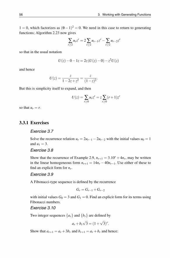
56 3. Working with Generating Functions
1 = 0, which factorizes as (θ− 1)2 = 0. We need in this case to return to generatingfunctions; Algorithm 2.23 now gives
∑r≥2
urzr = 2 ∑
r≥2ur−1zr − ∑
r≥2ur−2zr
so that in the usual notation
U(z)−0−1z = 2z(U(z)−0)− z2U(z)
and hence
U(z) =z
1−2z+ z2 =z
(1− z)2 .
But this is simplicity itself to expand, and then
U(z) = ∑r≥0
urzr = z ∑
r≥0
(r +1)zr
so that ur = r.
3.3.1 Exercises
Exercise 3.7
Solve the recurrence relation ur = 2ur−1 −2ur−2 with the initial values u0 = 1and u1 = 3.
Exercise 3.8
Show that the recurrence of Example 2.9, nr+1 = 3.10r + 4nr, may be writtenin the linear homogeneous form nr+1 = 14nr − 40nr−1. Use either of these tofind an explicit form for nr.
Exercise 3.9
A Fibonacci-type sequence is defined by the recurrence
Gr = Gr−1 +Gr−2
with initial values G0 = 3 and G1 = 0. Find an explicit form for its terms usingFibonacci numbers.
Exercise 3.10
Two integer sequences {ar} and {br} are defined by
ar +br
√3 = (1+
√3)r.
Show that ar+1 = ar +3br and br+1 = ar +br and hence:

3.4 Miscellaneous Exercises 57
(i) find the single recurrence (with appropriate initial values) that each se-quence satisfies;
(ii) find an explicit form for the terms of each sequence.
Exercise 3.11
In Exercise 2.20 you found a recurrence relation for the number of tilings: fr =2 fr−1 +3 fr−2. Find an explicit form for the number of tilings.
3.4 Miscellaneous Exercises
Exercise 3.12
The sequence {ar} is made up of terms in which ar = 3ar−1 +2r for r � 1, andinitial term a0 = 1. Convert this into a generating function and hence determinean explicit form for each of its terms.
Exercise 3.13
In a permutation π of the set {1,2,3, · · · r} the “distance” an element i movesis given by the expression |π(i)− i|. If {ur} counts the number of permutationsthat move no more than one unit, find an explicit form for the terms of thissequence.
Exercise 3.14
Let wr be the number of “words” (alphabetic strings) of length r formed fromthe letters {e,a, t} in which e is always followed by a. Construct the recurrencerelation satisfied by the sequence {wr} and hence find an explicit form for itsterms.
Exercise 3.15
Suppose that there are wr “words” of length r made up from the alphabet{v,e,r,y}, in which there are no consecutive repetition of letters. Find a re-currence for the sequence {wr} and hence find an explicit form for its terms.
Exercise 3.16
Given that φ1 + φ2 = 1, and φ1φ2 = −1 where φ1 and φ2 are as defined inExample 3.4, show that φ2
1 = φ1 + 1 and find the corresponding result for φ2.Hence prove that φr
1 = Frφ1 +Fr−1.
Exercise 3.17
The recurrenceFr(w) = wFr−1(w)+Fr−2(w)

58 3. Working with Generating Functions
with the initial terms F0(w) = 1 and F1(w) = w defines a sequence of polyno-mials {Fr(w)}. Show that:
(i) F2(w) = w2 +1 and F3 = w3 +2w;
(ii) the characteristic equation of the polynomial sequence is
θ2 −wθ−1 = 0;
(iii) the polynomials are given by
Fr(w) =
(w+
√w2 +4
)r+1−
(w−
√w2 +4
)r+1
2r+1√
w2 +4;
(iv) Fr+1 = Fr(1).
Exercise 3.18
Prove Theorem 3.14.
Exercise 3.19
Let nr denote the number of non-negative integer solutions of the equationx+2y+3z = r. By using partial fractions to rewrite the expression,
1− z6
(1− z)(1− z2)(1− z3),
show that nr obeys the surprising recurrence
nr −nr−6 = r (r � 7).

4Permutation Groups
4.1 Introduction to Groups
It might seem odd that we want to discuss group theory in a book on enumeration butit will turn out to be an important tool. If we are counting the number of arrangementsof a set of objects, we might wish to count two arrangements which are symmetrical asbeing the same. A simple example is that of a bracelet made up of different colouredbeads. It then makes sense to count two arrangements of the beads as the same if onecan be rotated into the other.
We will assume a basic knowledge of the definition of groups as well as an abilityto use them in a simple way. This can all be found in one or two books as part of thisseries. So we assume that readers are familiar with the following definitions.
Definition 4.1 (Subgroup)
Let G be a group and let H be a subset of G. If H is a group with respect to the samelaw of composition then H is called a subgroup of G.
Definition 4.2 (Order of group)
Let G be a group. If the number of elements in G, denoted by |G|, is finite, the groupis said to be a finite group. Otherwise the group is said to be infinite. If G is a finitegroup then the order of G is the size of the set G. If g ∈ G, then g is said to have finiteorder if the subgroup generated by g is finite.
A. Camina, B. Lewis, An Introduction to Enumeration,Springer Undergraduate Mathematics Series,DOI 10.1007/978-0-85729-600-9 4, © Springer-Verlag London Limited 2011
59

60 4. Permutation Groups
Definition 4.3 (Normal subgroup)
Let G be a group and let H be a subgroup of G. If gH = Hg for all g ∈ G, then H iscalled a normal subgroup of G.
Definition 4.4 (Homomorphism)
Let G and H be groups. A homomorphism from G to H is a mapping φ : H → H sothat φ(xy) = φ(x)φ(y) for all pairs x, f ∈ G. The set {x ∈ G : φ(x) = 1} is called thekernel of φ.
If φ is one–one and onto then φ is called an isomorphism.
An important observation is that the kernel is a normal subgroup of G: see Exer-cise 4.3.
Definition 4.5 (Cosets)
Let G be a group and let H be a subgroup of G. Let x ∈ G and consider the set Hx ={hx : h ∈ H}. This is called a right coset of H in G.
Similarly we define a left coset as xH = {xh : h ∈ H}. The term coset means eithera left coset or a right coset.
Theorem 4.6
Let G be a group and H a subgroup of G. Then the cosets of H partition G into sets ofequal cardinality. Thus if G is finite, |H| divides |G|.
The number of cosets is called the index of H in G. This is usually denoted by [G : H].This result is sometimes known as Lagrange’s Theorem, though there is no evi-
dence that he either knew or proved it. We will prove this in Proposition 4.49.
4.1.1 Exercises
Exercise 4.1
Let G be a group. Show that the intersection of subgroups is a subgroup. Henceshow that for any subset X there is a unique smallest subgroup containing X .This is called the subgroup generated by X and is written 〈X〉.Exercise 4.2
Let G be a group. Show that g ∈ G has order n ∈ N, if and only if n is the leastpositive integer such that gn = 1.

4.2 The Symmetric Group 61
Exercise 4.3
Let G and H be groups and let φ : G → H be a homomorphism between them.
(i) Show that the kernel of φ is a normal subgroup.
(ii) Show that if g ∈ G has order n then order of φ(g) divides n.
Exercise 4.4
Let G be a group and assume the order of G is a prime number. Show that Ghas only two subgroups.
Exercise 4.5
Let p be a prime number. Prove that any two groups of order p are isomorphic.
4.2 The Symmetric Group
In this section we define the symmetric group and look at some of its properties. Webegin by noting the following result.
Lemma 4.7
The composition of functions is associative.
Proof
Let V, X , Y and Z be sets and let f : V → X , g : X →Y and h : Y → Z all be functions.Choose y ∈ Y then
((hg) f )(y) = (hg)( f (y)) = (h(g( f (y)) = ((h)(g f )(y) = ((h(g f )(y)).
All this says is that if we map y by h and then by f g it is the same as mapping y bygh and then by f , which is just the same as mapping y by f , then by g and finally byh.
Note: writing composition of functions as ◦ this says that h◦ (g◦h) = (h◦g)◦ ( f ).
Proposition 4.8
Let X be a set. The set of permutations of X with multiplication defined by composi-tion of functions is a group.
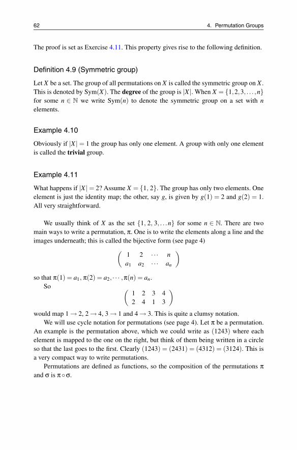
62 4. Permutation Groups
The proof is set as Exercise 4.11. This property gives rise to the following definition.
Definition 4.9 (Symmetric group)
Let X be a set. The group of all permutations on X is called the symmetric group on X .This is denoted by Sym(X). The degree of the group is |X |. When X = {1,2,3, . . . ,n}for some n ∈ N we write Sym(n) to denote the symmetric group on a set with nelements.
Example 4.10
Obviously if |X | = 1 the group has only one element. A group with only one elementis called the trivial group.
Example 4.11
What happens if |X | = 2? Assume X = {1, 2}. The group has only two elements. Oneelement is just the identity map; the other, say g, is given by g(1) = 2 and g(2) = 1.All very straightforward.
We usually think of X as the set {1, 2, 3, . . .n} for some n ∈ N. There are twomain ways to write a permutation, π. One is to write the elements along a line and theimages underneath; this is called the bijective form (see page 4)
(1 2 · · · na1 a2 · · · an
)
so that π(1) = a1, π(2) = a2, · · · ,π(n) = an.So (
1 2 3 42 4 1 3
)
would map 1 → 2, 2 → 4, 3 → 1 and 4 → 3. This is quite a clumsy notation.We will use cycle notation for permutations (see page 4). Let π be a permutation.
An example is the permutation above, which we could write as (1243) where eachelement is mapped to the one on the right, but think of them being written in a circleso that the last goes to the first. Clearly (1243) = (2431) = (4312) = (3124). This isa very compact way to write permutations.
Permutations are defined as functions, so the composition of the permutations πand σ is π◦σ.
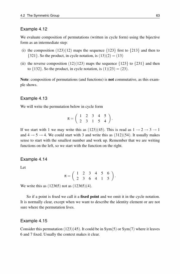
4.2 The Symmetric Group 63
Example 4.12
We evaluate composition of permutations (written in cycle form) using the bijectiveform as an intermediate step:
(i) the composition (123)(12) maps the sequence {123} first to {213} and then to{321}. So the product, in cycle notation, is (13)(2) = (13)
(ii) the reverse composition (12)(123) maps the sequence {123} to {231} and thento {132}. So the product, in cycle notation, is (1)(23) = (23).
Note: composition of permutations (and functions) is not commutative, as this exam-ple shows.
Example 4.13
We will write the permutation below in cycle form
π =(
1 2 3 4 52 3 1 5 4
).
If we start with 1 we may write this as (123)(45). This is read as 1 → 2 → 3 → 1and 4 → 5 → 4. We could start with 3 and write this as (312)(54). It usually makessense to start with the smallest number and work up. Remember that we are writingfunctions on the left, so we start with the function on the right.
Example 4.14
Let
π =(
1 2 3 4 5 62 3 6 4 1 5
).
We write this as (12365) not as (12365)(4).
So if a point is fixed we call it a fixed point and we omit it in the cycle notation.It is normally clear, except when we want to describe the identity element or are notsure where the permutation lives.
Example 4.15
Consider this permutation (123)(45). It could be in Sym(5) or Sym(7) where it leaves6 and 7 fixed. Usually the context makes it clear.

64 4. Permutation Groups
The cycle notation gives us a lot of information about the permutation that it rep-resents. The next lemma shows that we can always write permutations as a product ofdisjoint cycles; see page 4.
Lemma 4.16
Let g ∈ Sym(n). Then g can be written as a product of disjoint cycles, say
(a1 a2 . . . ar1)(ar1+1 ar1+2 . . .ar1+r2) · · ·(ar1+···+rc−1 . . .ar1+···+rc);
Here the sets of entries in each cycle are disjoint and the cycles have lengths r1, r2,. . . ,rc. Further the order of g is lcm(r1,r2, . . . ,rc).
Proof
Choose an element, i, not fixed by g. If there isn’t one, then g is the identity so weare done. Begin by writing the cycle (i g(i) g2(i) . . .). We know that at some stage anelement will be repeated, as there are only finitely many elements. Let s be the powerof g which gives the first repeat. So gs(i) = gt(i) for some 0 ≤ t < s.
Note that gs−t(i) = g0(i) = i, since g0 is the identity. Since s was chosen to bethe first repeat t = 0 and gs(i) = i. Further the points i,g(i),g2(i), . . . ,gs−1(i) are alldistinct. So (ig(i) . . . gs−1(i)) is a cycle.
Let Y = {1,2, . . . ,n} \ {(i,g(i), . . . ,gs−1(i)}. If there are no elements in Y movedby g we are done. If not choose j ∈ Y so that g( j) �= j. Repeat the process where wehave u so that ( j,g( j), . . . ,gu−1( j)).
We now have to show that these two cycles are disjoint. So assume false and thenwe get ga(i) = gb( j) for some a,b, but then j = ga−b(i) so j would be part of the firstcycle, which is false.
Let π = (a1a2 . . .ar) be a cycle length r. Then πr(ai) = ai,1 ≤ i ≤ r. So π has orderr. The final part of the lemma follows immediately.
We say that a cycle of length r is an r-cycle. A cycle of length 2 is called a trans-position. The cycle structure of a permutation gives considerable information about apermutation. The next lemma counts how many permutations there are of each cyclestructure, but first we count how many permutations there are. We know from Theo-rem 1.7 that |Sym(n)| = n!.
Example 4.17
Let us count the number of permutations of each cycle type in the symmetric group ofdegree 4. We denote the cycle type of an element by a sequence ini where the element
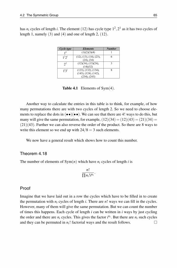
4.2 The Symmetric Group 65
has ni cycles of length i. The element (12) has cycle type 12,21 as it has two cycles oflength 1, namely (3) and (4) and one of length 2, (12).
Table 4.1 Elements of Sym(4).
Another way to calculate the entries in this table is to think, for example, of howmany permutations there are with two cycles of length 2. So we need to choose ele-ments to replace the dots in (••)(••). We can see that there are 4! ways to do this, butmany will give the same permutation, for example, (12)(34) = (12)(43) = (21)(34) =(21)(43). Further we can also reverse the order of the product. So there are 8 ways towrite this element so we end up with 24/8 = 3 such elements.
We now have a general result which shows how to count this number.
Theorem 4.18
The number of elements of Sym(n) which have ni cycles of length i is
n!
∏ni!ini.
Proof
Imagine that we have laid out in a row the cycles which have to be filled in to createthe permutation with ni cycles of length i. There are n! ways we can fill in the cycles.However, many of them will give the same permutation. But we can count the numberof times this happens. Each cycle of length i can be written in i ways by just cyclingthe order and there are ni cycles. This gives the factor ini . But there are ni such cyclesand they can be permuted in ni! factorial ways and the result follows.

66 4. Permutation Groups
Example 4.19
Let us check the answers in the example above. The second line would give 4!/2!121!21
which is 24/4 = 6. The third line is 24/2!22 = 3.
Another important property of permutations is a number called its sign, which aswe will see counts the number of transpositions into which it can be decomposed.
Lemma 4.20
Let g ∈ Sym(n). Then
∏i< j
(g(i)−g( j)) = εg ∏i< j
(i− j),
where εg = ±1.
Proof
Since all the possible differences occur exactly once in each product we see that εg =±1.
Definition 4.21 (Sign of permutation)
The coefficient from the previous lemma, εg, is called the sign of g. If εg = 1 the g iscalled an even permutation and if εg = −1 the g is called an odd permutation.
Proposition 4.22
Let g, h ∈ Sym(n). Then εgh = εgεh. The set of even permutations form a normalsubgroup of index 2 called the Alternating Group.
Proof
We begin by defining ag for g ∈ Sym(n) to be equal to the number of pairs (i, j) ∈X ×X , i �= j so that g(i)−g( j) has a different sign from i− j. Then εg = (−1)ag . Notethat this number is not dependent on the ordering of the set X . So for any pairs g,h∈ G
εgh ∏i< j
(i− j) = ∏i< j
(gh(i)−gh( j))
since the ordering is irrelevant, this can be rewritten as
εg ∏i< j
(h(i)−h( j)) = εgεh ∏i< j
(i− j).

4.2 The Symmetric Group 67
Now we see that the map g→ εg is a homomorphism from G into the multiplicativegroup {+1,−1}. The kernel is exactly the set of even permutations, thus proving thelast part of the proposition.
Example 4.23
Consider Sym(n) and a transposition g = (i j). How many pairs, as in the previousproposition, will have their sign changed by the action of g? The answer is the pairsof the form (i,r) and (s, j) where i < r ≤ j and i ≤ s < j. There are 2( j− i)−1 suchchanges, so all transpositions are odd, somewhat oddly.
Definition 4.24 (Cyclic permutation)
A permutation which consists of one cycle of length r and cycles of length 1, is calleda cyclic permutation.
Lemma 4.25
A cyclic permutation can be written as as the product of r− 1 transpositions. Hencea cyclic permutation of length r is an odd permutation if r is even and is an evenpermutation if r is odd, where a cyclic permutation is one that consists of one cycle.
Proof
Let the cycle be (a1 a2 . . . ar). Note that
(a1 a2 . . . ar) = (a2 a3) · · ·(ar−1 ar)(a1 ar).
The result now follows from the previous example and proposition.
Since any permutation is a product of cycles then any permutation can be writtenas a product of transpositions. However, there are many different ways that this can bedone. The number always has the same parity because this determines the sign whichis an invariant of the permutation.
Lemma 4.26
The alternating group of degree n has order n!/2.
Proof
This follows immediately from Theorem 1.7 and Proposition 4.22.

68 4. Permutation Groups
Lemma 4.27
Any even permutation can be written as a product of three cycles.
Proof
We know that any permutation can be written as a product of transpositions. If the per-mutation is even, it can be written as a product of an even number of transpositions.We can group them in pairs and so we need to consider the product of two transposi-tions, say (ab)(cd). If {a,b}= {c,d} the product is the identity. If there are only threedistinct symbols, we can assume that the product is (ab)(ac). But (ab)(ac) = (acb).If they are all distinct, we get (ab)(cd) = (acb)(acd). So the proof is complete.
Definition 4.28 (A permutation group)
Let n be a natural number. A permutation group of degree n is a subgroup of Sym(n).
A given abstract group can be a permutation group in many different ways, evenof the same degree.
Example 4.29
Consider G = Sym(4). Then we can define two subgroups of G,
(i) A = {1,(12)(34),(13)(24),(14)(23)};
(ii) B = {1,(12),(12)(34),(34)}.
Both groups are abelian of order 4 and all non-trivial elements have order 2. So thetwo subgroups are isomorphic as abstract groups. However, they differ as permutationgroups: A has an element which maps 1 to 3 but B does not.
4.2.1 Exercises
Exercise 4.6
Show that Sym(4) has no elements of order 5.
Exercise 4.7
Show that the Sym(n) has no elements of order p for any prime p > n.
Exercise 4.8
For the group Sym(5) enumerate the different cycle types; calculate the orders

4.3 Group Actions 69
of such elements; count how many there are of each type.
Exercise 4.9
Show that the maximal order of an element in Sym(10) is 30.
Exercise 4.10
Find the generating function for the number of transpositions in the symmetricgroup.
4.3 Group Actions
Definition 4.30 (Group action)
Let G be a group and X be a set. Then we say that G acts on X , if for each g ∈ G thereis a mapping φ(g) : X → X so that
(i) φ(g)φ(h)(x) = φ(gh)(x), ∀x ∈ X and ∀g, h ∈ G and
(ii) φ(1)(x) = x,∀x ∈ X .
We see with this definition that φ(G) is a permutation group of degree |X |.
Example 4.31
If we take X as the set X = {1,2,3, . . . ,n} and the group G as the symmetric group onX . Then φ may be the identity. In fact this works for any permutation group.
Example 4.32 (Regular Action)
In this we make a group act on itself. So both the group and the set are G. We have todefine an action φ. So we define φ(g)(x) = gx. We also have to check the rules for anaction.
φ(g)φ(h)(x) = φ(g)(hx) = g(hx) = (gh)(x) = φ(gh)(x).
Also φ(1)(x) = 1x = x.
Example 4.33 (Conjugate Action)
Again we make a group act on itself. So both the group and the set are G. This timehowever, we define φ(g)(x) = gxg−1. The proof follows the proof in the exampleabove.

70 4. Permutation Groups
φ(gh)(x) = ghxh−1g−1 = g(hxh−1)g−1) = (gφ(h)(x)g−1 = φ(g)(φ(h))(x) = φ(gh)(x).Also φ(1)(x) = 1x = x.
Definition 4.34 (Conjugate)
Let G be a group and let x and y be two elements of G. Then x and y are said to beconjugate if there exists g ∈ G so that gxg−1 = y.
Note: In many books the definition would be g−1xg = y. As we write functions onthe right we choose the form gxg−1 = y. However, they are the same relationship as(g−1)−1xg−1 = y.
Example 4.35
In this we make a group act on subsets of itself, so we define X = {Y : Y ⊆ X}. Thenφ(g)(Y ) = gY .
Example 4.36
Consider G = Sym(4). Then we can define two subgroups of G.
(i) A = {1,(12)(34),(13)(24),(14)(23)} and
(ii) B = {1,(12),(12)(34),(34)}.
This is taken from Example 4.29. Consider polynomials in four indeterminates X1,X2,
X3 and X4 (see Section 2.1) and let A and B act on them as follows:
gP(X1,X2,X3,X4) = P(Xg(1),Xg(2),Xg(3),Xg(4)
whenever g is in G.Let P = X1X3 + X2X4 and see what happens as we act on this polynomial. For all
a ∈ A we have a(P) = P. If we consider
(12)P = X2X3 +X1X4
we see that (12)P �= P. This is another illustration of the difference of the two permu-tation properties of A and B.
Example 4.37
Let X1,X2, . . . ,Xn be n indeterminates (see Section 2.1) and let G be a permutationgroup of degree n. Let F be a field and let X = F [X1,X2, . . . ,Xn]. We let G act on X by

4.3 Group Actions 71
permuting the suffices, that is if P(X1,X2, . . . ,Xn) is a polynomial and g ∈ G then gPis defined to be the polynomial P(Xg(1),Xg(2), . . . ,Xg(n)).
This gives an alternative way of defining the sign of a permutation. Let the poly-nomial P be ∏(Xi −Xj). Then the sign is given by gP = εgP, since g(P) = ±P. As Gacts on X we get the multiplicative property, see Proposition 4.22.
An important class of examples, which we will be particularly interested in, comefrom geometry, when we examine the groups of symmetries which fix a particu-lar shape or configuration. These groups are isometries of Euclidean space, that isthose mappings which fix distances. Our examples will come from two- and three-dimensional Euclidean space.
Example 4.38
Let G be the group of symmetries of the regular n-gon. First suppose that X is the setof vertices of the n-gon. Then G has a group action on X . G has order 2n. Also G hasa group action on the edges.
Definition 4.39 (Cyclic groups)
A group G with the property that G has an element G so that every element in G is apower of g is called a cyclic.
We now give an example.
Example 4.40
Let C be the group of rotational symmetries, of the regular n-gon. Now the symmetrygiven by the reflection is not in C. Let ρ be the rotation through 2π/n radians. Thenevery element of C is just a power of ρ.
Cyclic groups are particularly easy to study because of the generating element.Let G be cyclic of order n and let g generate G. So the order of g is n. We know fromLagrange’s Theorem 4.6 that, if H is a subgroup of G, then |H| divides n. But in thiscase the converse holds. If d|n then gn/d has order d.
Example 4.41
Let T be a regular tetrahedron and let G be the group of symmetries of T . T has fourvertices, six edges and four faces. Thus G can be represented as a permutation groupof degree 4 and of degree 6 (see Figure 4.1).

72 4. Permutation Groups
Figure 4.1 Tetrahedron.
Definition 4.42 (Stabilizer and fixed points)
Let G act on a set X . Then:
(i) for x ∈ X then the stabilizer of x in G is Gx = {g ∈ G : g(x) = x};
(ii) if g ∈ G the set of fixed points is defined by Fix(g) = {x ∈ X : g(x) = x}.
Lemma 4.43
Let G act on a set X . Then Gx is a subgroup of G for all x ∈ G.
Proof
Note that 1(x) = x, so 1 ∈ Gx. Also, if g ∈ Gx, then x = 1(x) = g−1g(x) = x. Sox = g(x) = g−1(x) and g−1 ∈ Gx. Finally, if h ∈ Gx, then gh(x) = g(x) = x.
4.3.1 Exercises
Exercise 4.11
Let X be a set. The set of permutations of X with multiplication defined bycomposition of functions is a group. (This is Proposition 4.8.)
Exercise 4.12
Let G be a finite group. Let X be any subset of G. Show that the set {g ∈ G :gX = X} is a subgroup of G.
Exercise 4.13
Let C be a cyclic group of order n. Let c ∈ C generate C. Prove the assertions
in Example 4.39 that c has order n and that if d|n then cn/d has order d.
4.4 Counting Subgroups 73
Exercise 4.14
Show that the symmetry group of the tetrahedron is isomorphic to Sym(4).
Exercise 4.15
Show that in the symmetric group of degree n, conjugacy is determined by thecycle structure, that is, if g, h ∈ Sym(n), then g and h are conjugate, if and onlyif g and h have the some cycle structure.
Exercise 4.16
Consider the action of Sym(4) on the indeterminates X1,X2,X3,X4. Find thesubgroup of Sym(4) which leaves the polynomial X1 + X2 − X3 − X4 fixed.Further find a polynomial fixed by the element (1234), but not by the wholegroup.
Exercise 4.17
Let G be a permutation group of degree n. Let p be a prime such that p doesnot divide n. Prove that any element of order p has to fix at least one point.
4.4 Counting Subgroups
We are almost ready to exploit group actions in counting arguments that involve ge-ometry. But first some useful notation. If Y is a subset of X and H is a subset of G wewrite H(Y ) = {h(y) : h ∈ H and y ∈ Y}. If either H or Y consists of a single elementwe drop the set notation, so if H = {h} we write h(Y ).
Definition 4.44 (Orbit of a group)
Let G act on X . An orbit of G is a subset Y ⊂ X such that
(i) G(Y ) = Y ,
(ii) Y is non-empty and
(iii) if /0 �⊆U �⊆ Y then G(U) �= U .
Lemma 4.45
If x ∈ X then G(x) is an orbit of G.

74 4. Permutation Groups
Proof
Let y ∈ G(x). Then there is an element h ∈ G so that y = h(x) but now g(y) = gh(x) =(gh)(x) ∈ G(x) ∀g ∈ G. Clearly if /0 �⊆ U �⊆ G(x) and u ∈ U then u = k(x) for somek ∈ G. But now x = k−1k(x) so U = G(x).
Lemma 4.46
Let G be a finite group and let G act on X . Define a relation, R , on X by xR y, if andonly if there exists g ∈ G with g(x) = y. Then R is an equivalence relation and theorbits are just the equivalence classes.
Proof
Let x, y ∈ X with xR y. Then there is an element g ∈ G so that y = g(x). So g−1(y) = x.So yR x. Now assume yR z, then there exists h ∈ G with z = h(y). So z = hg(x) and soxR z. Since reflexivity is obvious we have that R is an equivalence relation. Note thatG(x) is just the equivalence class of x.
The next example is important.
Example 4.47
Let G be a group and H a subgroup of G. In this case we let X be the set of left cosets{xH : x ∈ G}. The action is defined by xH → gxH.
We now prove a key result which relates orbits of elements to cosets of subgroups.
Theorem 4.48 (Orbit-Stabilizer Theorem)
Let G be a group and let G act on X . Let x ∈ X . Then there is a bijection between theelements of G(x) and the cosets of Gx.
Proof
We need to define a map ψ from G(x) to the cosets of Gx. Let y ∈ G(x) and let g ∈ Gbe such that g(x) = y, then define ψ(y) = gGx. We have to show that ψ is well-definedand that it is a bijection.
To show that it is well-defined, consider h ∈ G so that h(x) = y = g(x). Thenh−1g(x) = x so h−1g ∈ Gx. So hGx = gGx and ψ is well-defined.
To show that ψ is an injection assume ψ(y) = ψ(z). So if g(x) = y and h(x) = z

4.4 Counting Subgroups 75
then hGx = gGx and h−1g(x) = x. But then z = h(x) = g(x) = y and ψ is an injection.Finally we have to show that ψ is onto. Let gGx be any coset of Gx and let y = g(x) sothen ψ(y) = gGx.
We now use this to give a proof of Theorem 4.6.
Proposition 4.49
Let G be a finite group and let H be a subgroup of G. Then the order of H divides theorder of G.
Proof
We show that given any coset gH there is a bijection, ψ between gH and H. For anyk ∈ gH there is unique h ∈ H with k = gh. Define ψ(h) = k. It is easy to see that ψ iswell-defined and that it is a bijection. Since G is the disjoint union of the cosets of Hand there are m cosets we see that |G| = m|H|.
The number of cosets of a subgroup in a group is called the index and is written[G : H]. Hence, the previous theorem we write |G| = |H|[G : H]. This result, com-bined with the previous one, has far-reaching consequences, one of which is the classequation for finite groups.
Theorem 4.50 (Class equation for a finite group)
Let G be a finite group and let C1,C2, . . .Ck be the distinct conjugacy classes of G.Then |Ci| divides |G| for 1 ≤ i ≤ k. Further
|G| =k
∑1
|Ci|.
Proof
We note that the conjugacy classes are just the orbits of G acting on G by the conjugateaction, Example 4.33. So by Theorem 4.48 and Proposition 4.49 we get the result.
A simple corollary gives a well-known result about p-groups, which requires twodefinitions.
76 4. Permutation Groups
Definition 4.51 (A p-group)
Given a prime p, a finite p-group is a finite group whose order is a power of p.
Definition 4.52 (Centre of a group)
The centre of a group is the set of all elements which commute with all elements ofthe group: {z : zx = xz∀x ∈ G}.
Note the identity is always in the centre so we say that the centre is non-trivial if itcontains at least two elements.
Corollary 4.53
Let p be a prime and G be a finite p-group then the centre of G is non-trivial.
Proof
We observe that z is in the centre of G if and only if the conjugacy class of z is just {z}and so has size 1. Let |G| = pa. Now by the equation above
pa =k
∑1
|Ci|,
where C1,C2, . . .Ck are the distinct conjugacy classes of G. If we let C1 be the con-jugacy class that consists of the identity element then |C1| = 1. Note, by the theoremabove each |Ci| divides pa. So at least one other Ci has |Ci| = 1. So this conjugacyclass consists of one non-identity element which is in the centre.
Another consequence is an alternative proof of Sylow’s First Theorem.
Theorem 4.54 (Sylow’s First Theorem)
Let G be a finite group of order pam where p is a prime, a and m are natural numberswith gcd(p,m) = 1. Then there exists a subgroup of G order pa. Such a subgroup iscalled a Sylow p-subgroup.
Proof
Let X be the set of subsets of G of size pa. There are(pam
pa
)such subsets,Theorem 1.9
and such a number is coprime to p (see Exercise 4.26). Let G act on X by right
4.5 Miscellaneous Exercises 77
multiplication. There must be a an orbit of size coprime to p. Let X be a subset insuch an orbit and consider GX the stabilizer of this subset.
Now XGX = X by the definition of GX . So X =∪x∈X xGX and we can see that X isa union of cosets of GX . So the order of GX divides the size of X . So |GX | divides pa.But [G : GX ] is prime to p by Theorem 4.48. So pa divides |GX | and hence |GX | = pa
and the theorem is proved.
4.4.1 Exercises
Exercise 4.18
Show that in Definition 4.30 for each g ∈ G the mapping φ(g) is a permutationof X .
Exercise 4.19
Consider, as in Example 4.32, the action of G on G but define φ(g)(x) = xg−1.Prove that this is an action. Explain why the inverse is used.
Exercise 4.20
Let g ∈ Sym(n). Consider the subgroup, say G, generated by g. Show that thecycles of g correspond to the orbits of G, that is if (a1,a2, . . . ,ar) is a cycle ofg then {a1,a2, . . . ,ar} is an orbit of G.
Exercise 4.21
Calculate the order of the symmetry group of the cube acting on its vertices.
Exercise 4.22
Let G be a finite group of order n. By rewriting the class equation as
1 =1n
+n1
n+ · · ·+ nr
n,
where there are r +1 conjugacy classes of sizes 1,n1, . . . ,nr, show that if thereare only two conjugacy classes then n = 2. Further if there are only three con-jugacy classes then n = 6.
4.5 Miscellaneous Exercises
Exercise 4.23
Let p be a prime and let G be a permutation group whose order is a power ofp. Show that each orbit of G has to be a p-power.

78 4. Permutation Groups
Exercise 4.24
Let G act on a set X of size n. Let Xr be the set of sequences of elements of Xof length r. Show that we can define an action on Xr by g(x1,x2,x3, . . . ,xr) =(g(x1),g(x2), . . . ,g(xr). (This is known as the diagonal action.)
Prove that, when G is the symmetric group action on X = {1,2, . . . ,n}, thereare two orbits of G on X2 and five orbits on X3. What is the general result?
Exercise 4.25
Let p be a prime and let n be a natural number. Show that the order of theSylow p-subgroup of Sym(n) is given by
∑k
npk �.
Exercise 4.26
Let p be a prime and a and b be natural numbers with gcd(pa,m) = 1. Prove
that gcd((pam
pa
), p) = 1.
Exercise 4.27
Show that the relationship of conjugacy is an equivalence relation.

5Matrices, Sequences and Sums
5.1 Pascal’s Triangle and Enumeration
This triangle – better described as an array – is associated with the Binomial Theorem2.1; this expresses the powers of (1+ z) in terms of successive powers of z:
(1+ z)r = ∑k≥0
(rk
)zk.
The next result shows that the coefficients involved represent the number of ways ofchoosing k elements from r, as assumed in the first chapter.
Theorem 5.1 (Choosing k objects from r)
The Binomial coefficient(r
k
)enumerates the number of ways of making a choice of k
objects (without repetition) from r distinct objects.
Proof
We can write
(1+ z)r =
r terms︷ ︸︸ ︷(1+ z)(1+ z) · · ·(1+ z) .
To form a term in zk, on the right we must select a “z” from k brackets and there are rsuch brackets to choose from. So the resulting coefficient of zk is simply the numberof ways that this choice can be made.
A. Camina, B. Lewis, An Introduction to Enumeration,Springer Undergraduate Mathematics Series,DOI 10.1007/978-0-85729-600-9 5, © Springer-Verlag London Limited 2011
79

80 5. Matrices, Sequences and Sums
We are going to focus on the array made up from the Binomial coefficients. So ourfirst step is to write the Binomial Theorem in terms of matrices
⎛⎜⎜⎜⎜⎜⎝
11+ z
(1+ z)2
(1+ z)3
. . .
⎞⎟⎟⎟⎟⎟⎠
=
⎛⎜⎜⎜⎜⎜⎝
1 0 0 . .
1 1 0 . .
1 2 1 0 .
1 3 3 1 .
. . . . .
⎞⎟⎟⎟⎟⎟⎠
⎛⎜⎜⎜⎜⎜⎝
1zz2
z3
. . .
⎞⎟⎟⎟⎟⎟⎠
and Pascal’s triangle is the coefficient array that results. Pascal’s triangle is generatedby a recurrence relation.
Theorem 5.2 (Recurrence between terms of Pascal’s array)
The recurrence relation satisfied by the entries in Pascal’s array is(
r +1k
)=
(rk
)+
(r
k−1
).
Proof
Using the Binomial Theorem we can write
(1+ z)r+1 = ∑k≥0
(r +1
k
)zk = (1+ z) ∑
k≥0
(rk
)zk
and then comparing coefficients of zk in each of the sums gives
(r +1
k
)=
(rk
)+
(r
k−1
)
exactly as required.
The terms that make up the array have many properties. An obvious property isthe nature of the terms that make up each of the columns. For example, the first col-umn consists of units; the non-zero terms in the second are simply natural numbers{1,2,3, . . .}, while the non-zero terms in the third column are the triangular numbers{1,3,6,10, . . .}. The non-zero terms in the next column consist of the so-called pyra-midal numbers {1,4,10,20,35, . . .}. This sequence of sequences, which has termsthat are partial sums of the sequence that precedes it, is the result of another basicproperty of the array.

5.1 Pascal’s Triangle and Enumeration 81
Theorem 5.3 (Partial sums of columns of Pascal’s array)
The partial sum of the terms in one column of Pascal’s array is the term in the nextcolumn one below the bottom term of the partial sum:(
r +1k +1
)=
r
∑l=k
(lk
).
Proof
Using the basic recurrence of Theorem 5.2 repeatedly we have(r +1k +1
)=
(rk
)+
(r
k +1
)
=(
rk
)+
((r−1
k
)+
(r−1k +1
))
· · ·
=(
rk
)+
(r−1
k
)+ · · ·+
(kk
)
=r
∑l=k
(lk
).
as required.
5.1.1 Exercises
Exercise 5.1
Prove the identity ∑k≥0(k +1)(r
k
)= (r +2)2r−1.
Exercise 5.2
Prove by an enumerative argument that k(r
k
)= r
(r−1k−1
).
Exercise 5.3
Prove, using an enumerative argument, that(r+1
k
)=
(rk
)+
( rk−1
). Deduce that
the upward diagonal sums of terms in Pascal’s triangle are Fibonacci numbers(Theorem 3.9).
Exercise 5.4
Show, using an enumerative argument, that(r
l
)(r−lk−l
)=
(rk
)(kl
).
Exercise 5.5
Prove, using an enumerative argument, that(r
k
)= ∑l≥0
(ml
)(r−mk−l
)for 0≤m≤ r.
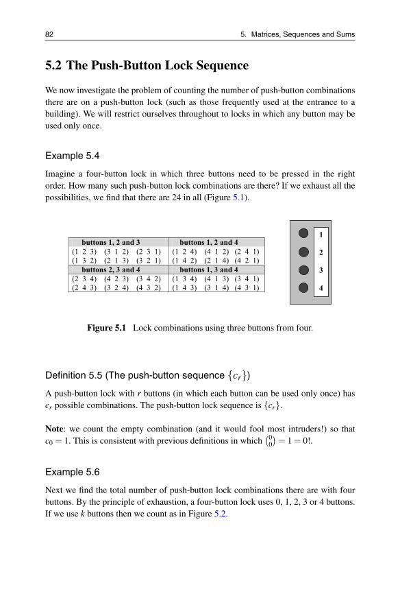
82 5. Matrices, Sequences and Sums
5.2 The Push-Button Lock Sequence
We now investigate the problem of counting the number of push-button combinationsthere are on a push-button lock (such as those frequently used at the entrance to abuilding). We will restrict ourselves throughout to locks in which any button may beused only once.
Example 5.4
Imagine a four-button lock in which three buttons need to be pressed in the rightorder. How many such push-button lock combinations are there? If we exhaust all thepossibilities, we find that there are 24 in all (Figure 5.1).
Figure 5.1 Lock combinations using three buttons from four.
Definition 5.5 (The push-button sequence {cr})
A push-button lock with r buttons (in which each button can be used only once) hascr possible combinations. The push-button lock sequence is {cr}.
Note: we count the empty combination (and it would fool most intruders!) so thatc0 = 1. This is consistent with previous definitions in which
(00
)= 1 = 0!.
Example 5.6
Next we find the total number of push-button lock combinations there are with fourbuttons. By the principle of exhaustion, a four-button lock uses 0, 1, 2, 3 or 4 buttons.If we use k buttons then we count as in Figure 5.2.

5.2 The Push-Button Lock Sequence 83
Figure 5.2 Lock combinations with k buttons.
In all then, the number of push-button lock combinations is
∑k≥0
(4k
)k! =
(40
)0!+
(41
)1!+
(42
)2!+
(43
)3!+
(44
)4!
= 1+4+12+24+24 = 65.
An extension of this enumerative method proves the following result.
Theorem 5.7 (Explicit form for terms of the sequence {cr})
A push-button lock with r buttons (in which each button can be used only once) has
cr = ∑k≥0
(rk
)k!
possible combinations and the sequence has the initial terms
{cr} = {1,2,5,16,65,326, . . .}.
5.2.1 Exercises
Exercise 5.6
Prove, using the previous theorem and Exercise 5.2, that a recurrence satisfiedby the push-button lock sequence {cr} is cr = rcr−1 + 1 with the initial valuec0 = 1. Now prove this with an enumerative argument.
Exercise 5.7
Prove that another recurrence relation satisfied by the sequence of push-buttonlocks is cr+1 = (r +2)cr − rcr−1.

84 5. Matrices, Sequences and Sums
Exercise 5.8
Give an inductive argument for the recurrence
r! = ∑k≥0
(−1)r−k(
rk
)ck.
Exercise 5.9
The push-button lock sequence {cr} now satisfies the two indentities
(i) cr = ∑k≥0(r
k
)k!;
(ii) r! = ∑k≥0(−1)r−k(r
k
)ck.
The derangement sequence {dr} also satisfies two identities. Each identity isan adaptation of Example 1.27 and Equation (1.2), respectively,
(i) dr = ∑k≥0(−1)r−k(r
k
)k!;
(ii) r! = ∑k≥0(r
k
)dk.
Write each of these four expressions in matrix form.
5.3 Pascal’s Triangle as a Matrix
Once we begin to think of the array as a matrix, a formidable problem arises: the arrayis unbounded. Surprisingly, this causes no problems. Pascal’s triangle begins like this:
P =
⎛⎜⎜⎜⎜⎜⎝
1 0 0 . .
1 1 0 . .
1 2 1 0 .
1 3 3 1 .
. . . . .
⎞⎟⎟⎟⎟⎟⎠
Definition 5.8 (Pascal’s triangle as a matrix)
Pascal’s triangle is the infinite matrix P =((
rk
): r,k ≥ 0
). Notice that we number rows
and columns from 0 not 1.
Having acknowledged that we are dealing with an infinite matrix, a matrix that extendsindefinitely downwards and to the right, we also note that it has a special form.

5.3 Pascal’s Triangle as a Matrix 85
Definition 5.9 (Lower triangular matrix)
A lower triangular matrix M = (mr,k) is one in which mr,k = 0 if k > r.
Every lower triangular matrix (finite or infinite) has well-defined positive powers. Thisis simply the result of its lower triangular structure and an important property: everyrow of a lower triangular matrix has only a finite number of non-zero terms. Hencethe product of two lower triangular matrices is itself lower triangular. This means thatsuch multiplication – and hence powers – is always well-defined.
Negative powers can also be defined for such arrays whenever an inverse exists.Fortunately there is a simple condition that ensures this.
Lemma 5.10 (Determinant of a lower triangular matrix)
The determinant of a finite square lower triangular matrix is the product of the entrieson its leading diagonal.
Proof
We use induction. To seed this∣∣∣∣(
m0,0
m1,0 m1,1
)∣∣∣∣ = m0,0m1,1
and so it is true for 2× 2 lower triangular matrices. Now suppose the n× n lowertriangular matrix (mr,k) has the determinant m0,0.m1,1. · · ·mn,n. Then the n+1×n+1lower triangular matrix (mr,k) has the determinant:∣∣∣∣∣∣∣∣∣∣∣
⎛⎜⎜⎜⎜⎜⎝
m0,0
m1,0 m1,1
. .
. . . .
mn+1,0 mn+1,n+1
⎞⎟⎟⎟⎟⎟⎠
∣∣∣∣∣∣∣∣∣∣∣= m0,0
∣∣∣∣∣∣∣∣∣∣∣
⎛⎜⎜⎜⎜⎜⎝
m1,1
m2,1 m2,2
. .
. . . .
mn+1,0 mn+1,n+1
⎞⎟⎟⎟⎟⎟⎠
∣∣∣∣∣∣∣∣∣∣∣which, by hypothesis, is simply m0,0 (m1,1. · · ·mn+1,n+1), exactly as required for theinduction to succeed.
This means that so long as there are no zeros on the leading diagonal, the (finite)inverse exists and this leads directly to the inverse of the infinite array. In turn this leadsto any negative power of the array. We investigate the powers of Pascal’s triangle.
Theorem 5.11 (Inverse of Pascal’s matrix)
The inverse of Pascal’s triangle is given by P−1 =((−1)r−k(r
k
)).

86 5. Matrices, Sequences and Sums
Proof
The Binomial expansion
(1+ z)r = ∑k≥0
(rk
)zk (5.1)
expresses powers of (1 + z) in terms of powers of z. To find the inverse of Pascal’striangle we must invert this equation: that is, to express powers of z in terms of powersof (1+ z). The resulting coefficients will form an array that is the inverse of the Pascalarray. But Equation (5.1) may be transformed by z →−z−1 and becomes
(−1)rzr = ∑l≥0
(−1)l(
rl
)(1+ z)l .
This may be rewritten:
zr = ∑k≥0
(−1)r−k(
rk
)(1+ z)k (5.2)
Equation (5.2) is the required inverted form of Equation (5.1), and we conclude thatP−1 =
((−1)r−k
(rk
)).
The inverse has the same terms as Pascal’s matrix but with alternating signs – positiveif the indices r and k have the same parity and negative otherwise:
P−1 =
⎛⎜⎜⎜⎜⎜⎝
1 0 0 . .
−1 1 0 . .
1 −2 1 0 .
−1 3 −3 1 .
. . . . .
⎞⎟⎟⎟⎟⎟⎠
.
This means that the inverse of Pascal’s array is a signed copy of itself. Now look backat Exercise 5.9. We can make sense of the four identities there – they involve Pascal’striangle and its inverse. The derangement numbers {dr} satisfy the recurrence
r! = ∑k≥0
(rk
)dk
which may be written in the matrix form⎛⎜⎜⎜⎜⎜⎝
0!1!2!3!. . .
⎞⎟⎟⎟⎟⎟⎠
=
⎛⎜⎜⎜⎜⎜⎝
1 0 0 . .
1 1 0 . .
1 2 1 0 .
1 3 3 1 .
. . . . .
⎞⎟⎟⎟⎟⎟⎠
⎛⎜⎜⎜⎜⎜⎝
d0
d1
d2
d3
. . .
⎞⎟⎟⎟⎟⎟⎠
.
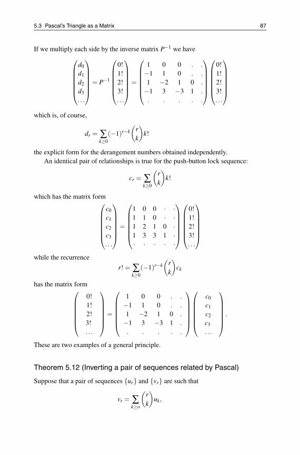
5.3 Pascal’s Triangle as a Matrix 87
If we multiply each side by the inverse matrix P−1 we have⎛⎜⎜⎜⎜⎜⎝
d0
d1
d2
d3
. . .
⎞⎟⎟⎟⎟⎟⎠
= P−1
⎛⎜⎜⎜⎜⎜⎝
0!1!2!3!. . .
⎞⎟⎟⎟⎟⎟⎠
=
⎛⎜⎜⎜⎜⎜⎝
1 0 0 . .
−1 1 0 . .
1 −2 1 0 .
−1 3 −3 1 .
. . . . .
⎞⎟⎟⎟⎟⎟⎠
⎛⎜⎜⎜⎜⎜⎝
0!1!2!3!. . .
⎞⎟⎟⎟⎟⎟⎠
which is, of course,
dr = ∑k≥0
(−1)r−k(
rk
)k!
the explicit form for the derangement numbers obtained independently.An identical pair of relationships is true for the push-button lock sequence:
cr = ∑k≥0
(rk
)k!
which has the matrix form⎛⎜⎜⎜⎜⎜⎝
c0
c1
c2
c3
. . .
⎞⎟⎟⎟⎟⎟⎠
=
⎛⎜⎜⎜⎜⎜⎝
1 0 0 · ·1 1 0 · ·1 2 1 0 ·1 3 3 1 ·· · · · ·
⎞⎟⎟⎟⎟⎟⎠
⎛⎜⎜⎜⎜⎜⎝
0!1!2!3!. . .
⎞⎟⎟⎟⎟⎟⎠
while the recurrence
r! = ∑k≥0
(−1)r−k(
rk
)ck
has the matrix form⎛⎜⎜⎜⎜⎜⎝
0!1!2!3!. . .
⎞⎟⎟⎟⎟⎟⎠
=
⎛⎜⎜⎜⎜⎜⎝
1 0 0 . .
−1 1 0 . .
1 −2 1 0 .
−1 3 −3 1 .
. . . . .
⎞⎟⎟⎟⎟⎟⎠
⎛⎜⎜⎜⎜⎜⎝
c0
c1
c2
c3
. . .
⎞⎟⎟⎟⎟⎟⎠
.
These are two examples of a general principle.
Theorem 5.12 (Inverting a pair of sequences related by Pascal)
Suppose that a pair of sequences {ur} and {vr} are such that
vr = ∑k≥o
(rk
)uk,

88 5. Matrices, Sequences and Sums
then we can invert this sum
ur = ∑k≥0
(−1)r−k(
rk
)vk.
Example 5.13
We can use this to illustrate a surprising property, and the inverse, of the Fibonaccinumbers that F2r = ∑k≥0
(rk
)Fk. Using Binet’s formula we have
∑k≥0
(rk
)Fk = ∑
k≥0
(rk
)1√5
(φk
1 −φk2
)=
1√5
(∑k≥0
(rk)φ
k1 − ∑
k≥0
(rk)φ
k2
).
Each sum inside the bracket is part of a Binomial expansion, and hence
∑k≥0
(rk
)Fk =
1√5
((1+φ1)r − (1+φ2)r) =1√5
((φ2
1)r − (φ2
2)r)
since φ2i = φi +1 for i = 1,2, see Exercise 3.16; this means that
∑k≥0
(rk
)Fk =
1√5
(φ2r
1 −φ2r2
)= F2r.
Using the previous theorem we can “invert” this sum and then we have the “dual”result
Fr = ∑k≥0
(−1)r−k(
rk
)F2k.
We continue our investigation of the powers of Pascal’s triangle.
Theorem 5.14 (The square of Pascal’s triangle)
The square of Pascal’s triangle is given by P2 = 2r−k(r
k
).
Proof
Again we manipulate the Binomial Theorem in two different ways and compare theresults. First
(2+ z)r = 2r(1+z2)r = 2r ∑
k≥0
(rk
)zk
2k = ∑k≥0
2r−k(
rk
)zk. (5.3)

5.3 Pascal’s Triangle as a Matrix 89
But we also have
(2+ z)r = (1+(1+ z))r = ∑l≥0
(rl
)(1+ z)l = ∑
l≥0
(rl
)∑k≥0
(lk
)zk
using the Binomial Theorem twice. The repeated sums are both finite, so we mayreverse them:
(2+ z)r = ∑k≥0
(∑l≥0
(rl
)(lk
))zk. (5.4)
Comparing the coefficients of zk in Equations (5.3) and (5.4) leads to
∑l≥0
(rl
)(lk
)= 2r−k
(rk
)
which is precisely the statement that P.P = P2 =(2r−k
(rk
))as required.
So the square of Pascal starts like this
P2 =
⎛⎜⎜⎜⎜⎜⎝
1 0 0 . .
2.1 1 0 . .
22.1 2.2 1 0 .
23.1 22.3 2.3 1 .
. . . . .
⎞⎟⎟⎟⎟⎟⎠
These results (based on the limited evidence of n = 1, n = −1 and n = 2) seem tosuggest a general result for powers of Pascal’s matrix: that Pn =
(nr−k
(rk
)).
Theorem 5.15 (Powers of Pascal’s matrix)
The integer powers of Pascal’s array (for n ∈ Z) are given by Pn =(nr−k
(rk
))where
we interpret P0 = I, the identity matrix.
Proof (For n positive)
We use induction. We have already established it for a positive “seed”. Suppose it is
true for n−1 so that Pn−1 =((n−1)r−k(r
k
)). Now
(n+ z)r = (1+(n−1+ z))r = ∑l≥0
(rl
)(n−1+ z)l = ∑
l≥0
(rl
)∑k≥0
(lk
)(n−1)l−kzk
= ∑k≥0
(∑l≥0
(rl
)(n−1)l−k
(lk
))zk.

90 5. Matrices, Sequences and Sums
The inner sum is simply the terms of the matrix product P.Pn−1. On the other hand
(n+ z)r = ∑k≥0
nr−k(
rk
)zk.
Comparing the coefficients of zk in each case establishes the result required. This proofis easily adapted to the case when n is negative.
This proves another general result about sequences related through powers of Pascal.
Theorem 5.16 (Pairs of sequences related by powers of Pascal)
Suppose that a pair of sequences {ur} and {vr} are such that
vr = ∑k≥0
nr−k(
rk
)uk,
where n ∈ Z. Then we can invert this sum
ur = ∑k≥0
(−n)r−k (rk)vk.
5.3.1 Exercises
Exercise 5.10
We may extend Theorem 5.15 from integers to rational powers; suppose weconsider the square root of Pascal’s array – that is a matrix whose square is justthe Pascal array. We might suppose that
√P =
(2k−r
(rk
))so that,
P12 =
⎛⎜⎜⎜⎜⎜⎜⎜⎝
1 .12 1 .14 1 1 .18
34
32 1 .
116
48
64
42 1 .
. . . . . .
⎞⎟⎟⎟⎟⎟⎟⎟⎠
.
Verify that (for initial rows and columns) P12 .P
12 = P.
Exercise 5.11
Show that the finite Pascal matrix
P3 =
⎛⎝1 0 0
1 1 01 2 1
⎞⎠
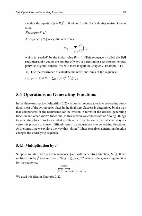
5.4 Operations on Generating Functions 91
satisfies the equation (I−P3)3 = 0 where I is the 3×3 identity matrix. Gener-alize.
Exercise 5.12
A sequence {Br} obeys the recurrence
Br+1 = ∑k≥0
(rk
)Bk
which is “seeded” by the initial value B0 = 1. (This sequence is called the Bellsequence and it counts the number of ways of partitioning a set into non-empty,pairwise disjoint, subsets. We will meet it again in Chapter 7, Example 7.14.
(i) Use the recurrence to calculate the next four terms of the sequence;
(ii) prove that Br = ∑k≥0 (−1)r−k(rk
)Bk+1.
5.4 Operations on Generating Functions
In the three-step recipe (Algorithm 2.23) to convert recurrences into generating func-tions, most of the action takes place in the final step. Success is determined by the waythat components of the recurrence can be written in terms of the desired generatingfunction and other known functions. In this section we concentrate on “doing” thingsto generating functions to see what results – the expectation is that later we may re-verse this process to convert difficult terms in a recurrence into generating functions.At the same time we explore the way that “doing” things to a given generating functionchanges the underlying sequence.
5.4.1 Multiplication by zk
Suppose we start with a given sequence {ur} with generating function, U(z). If wemultiply this by zk then we have zkU(z) = ∑r≥0 urzr+k which is the generating functionfor the sequence,
{k zeros︷ ︸︸ ︷
0,0, . . . ,0,u0,u1, . . .}.
We used this idea in Example 2.22.

92 5. Matrices, Sequences and Sums
5.4.2 The Product of Two Generating Functions
Consider the product of two generating function W (z) =U(z)V (z). The function W (z)is itself a generating function, but for what sequence? It turns out that the answer issimple and has powerful and varied applications.
Theorem 5.17 (The generating function product formula)
If W (z) = U(z)V (z), where U,V and W are the generating functions for the sequences{ur},{vr} and {wr}, then
wr =r
∑k=0
ukvr−k =r
∑k=0
ur−kvk.
Proof
The product of the two generating functions may be written out in the form:(u0 +u1z+u2z2 + · · ·+urz
r + · · ·)(
v0 + v1z+ v2z2 + · · ·+ vrzr + · · ·
).
If we want the coefficient of zr in this product, then we make it up from the sum ofthe products of pairs of terms taken one from each bracket. Moreover, the sum of thecorresponding powers of z, of which these pairs are the coefficients, must be r. So wehave:
wr = ∑k+l=r
ukvl
We may rewrite this in two (equivalent) forms
wr =r
∑k=0
ukvr−k =r
∑k=0
ur−kvk.
Example 5.18
We use the product of the Fibonacci and Lucas generating functions to derive an iden-tity. We may write the generating functions for the Fibonacci and Lucas sequences inthe forms,
∑r≥0
Frzr =
1√5
(1
1−φ1z− 1
1−φ2z
)and ∑
r≥0Lrz
r =(
11−φ1z
+1
1−φ2z
).

5.4 Operations on Generating Functions 93
(Using these forms of the generating functions, means fewer partial fractions later.)Now we take the product of these generating functions and then(
∑r≥0
Frzr
)(∑r≥0
Lrzr
)= 1√
5
(1
(1−φ1z)2 − 1(1−φ2z)2
).
Expand each term on the right,
(∑r≥0
Frzr
)(∑r≥0
Lrzr
)= 1√
5 ∑r≥0
(r +1)(φr1 −φr
2)zr = ∑r≥0
(r +1)Frzr.
We deduce, by the theorem above, that
r
∑k=0
FkLr−k = (r +1)Fr.
5.4.3 Partial Sums of a Sequence
If we are given a sequence {ur} it is of interest to find the sequence {vr} which has as
its terms the partial sums vr =r∑
k=0uk.
Theorem 5.19 (The sum formula)
Let {ur} be a sequence with a generating function U(z) then a generating function forthe sequence {vr} that consists of partial sums of the sequence {ur} is given by theproduct 1
1−zU(z).
Proof
This is a simple consequence of the generating function product formula, Theorem5.17. If we write V (z) = 1
1−zU(z) and then write these as power series, we have
∑r�0
vrzr =
(∑r�0
1zr
)(∑r�0
urzr
)
and then
vr =r
∑k=0
1.uk =r
∑k=0
uk
exactly as required.

94 5. Matrices, Sequences and Sums
The same idea can result in a different form of the partial sum – a “weighted” sum.If we multiply a generating function by a function that resembles 1
1−z then the resultis still a sum, but with a “weighting” according to the nature of the particular functionused.
Example 5.20
We take the product of the generating function of the Lucas numbers with the gener-
ating function 12−z to prove that
r∑
k=02kLk = 2r+1Fr+1. The generating function of the
Lucas numbers is given by ∑r≥0 Lrzr = 2−z1−z−z2 : if we multiply by the reciprocal of the
numerator on the right we have
12− z ∑
r≥0
Lrzr =1
1− z− z2 =1z
(z
1− z− z2
)=
1z ∑
r≥0
Frzr;
a slight rearrangement gives
1(1− z
2
) ∑r≥0
Lrzr =2z ∑
r≥0
Frzr.
The product on the left becomes(
∑r≥0
zr
2r
)(∑r≥0
Lrzr
)=
2z ∑
r≥0
Frzr
and then comparing coefficients of zr on either side (making use of the generatingfunction product formula, Theorem 5.17) gives
r
∑k=0
Lk
2r−k = 2Fr+1
and hence
r
∑k=0
2kLk = 2r+1Fr+1.
There are even more exotic ways that we can exploit this basic idea.
Example 5.21
We start with two given generating functions for {F2r } and {F2r},
∑r≥0
F2r zr =
z(1− z)(1+ z)(1−3z+ z2)
and ∑r≥0
F2rzr =
z1−3z+ z2 .

5.4 Operations on Generating Functions 95
The first generating function has the factor 1− z in the numerator, so we divide bothsides by it
(1
1− z
)∑r≥0
F2r zr =
z(1+ z)(1−3z+ z2)
.
Partial fractions now give
(1
1− z
)(∑r≥0
F2r zr
)=
15
(1+ z
1−3z+ z2 − 11+ z
)
=15
(1z
(z
1−3z+ z2
)+
z1−3z+ z2 − 1
1+ z
)
=15
(1z ∑
r≥0
F2rzr + ∑
r≥0
F2rzr − ∑
r≥0
(−1)rzr
).
Using the Sum formula, Theorem 5.19, provides the interesting identity
r
∑k=0
F2k =
15
(F2r+2 +F2r − (−1)r) .
5.4.4 The zD ≡ z ddz Operation
We have already made use of differentiation (Example 2.21). Now we look at repeateddifferentiation with an added ingredient.
Definition 5.22 (The Euler operation)
The zD operation (differentiate a function and then multiply by the argument) is calledthe Euler operation.
We apply the Euler operation to the function 11−z . We may expand the function as a
power series (when |z| < 1)
f (z) = ∑r≥0
zr =1
1− z.
A first application of the Euler operation gives
(zD) f (z) = ∑r≥0
rzr =z
(1− z)2

96 5. Matrices, Sequences and Sums
(We may differentiate term by term inside the disc of convergence of a power series.)Using the operation again gives
(zD)2 f (z) = ∑r≥0
r2zr = z.(1− z)2 + z.2.(1− z)
(1− z)4 =z+ z2
(1− z)3 .
Repeating the same operation one more time
(zD)3 f (z) = ∑r≥0
r3zr = z.(1+2z)(1− z)3 +(z+ z2).3.(1− z)2
(1− z)6 =z+4z2 + z3
(1− z)4 .
(5.5)
The coefficients appearing in the numerators follow a pattern that may be written inthe form of an array which continues:
⎛⎜⎜⎜⎜⎜⎜⎜⎜⎜⎝
1 .
0 1 .
0 1 1 .
0 1 4 1 .
0 1 11 11 1 .
0 1 26 66 26 1 .
. . . . . . .
⎞⎟⎟⎟⎟⎟⎟⎟⎟⎟⎠
.
Definition 5.23 (The Eulerian array)
The coefficients that appear in the numerators at each stage of the application of theEuler operation to the function 1
1−z are called Eulerian numbers and make up an arraycalled the Eulerian array. We write E =
(⟨rk
⟩).
Note: The symbol chosen to represent the Eulerian numbers mimics those used forBinomial coefficients. The indices representing the columns (k) and rows (r) are eachnumbered from zero; for example,
⟨00
⟩= 1,
⟨32
⟩= 4.
Theorem 5.24
The Eulerian numbers obey the recurrence⟨
n+1k
⟩= (n− k +2)
⟨n
k−1
⟩+ k
⟨nk
⟩.
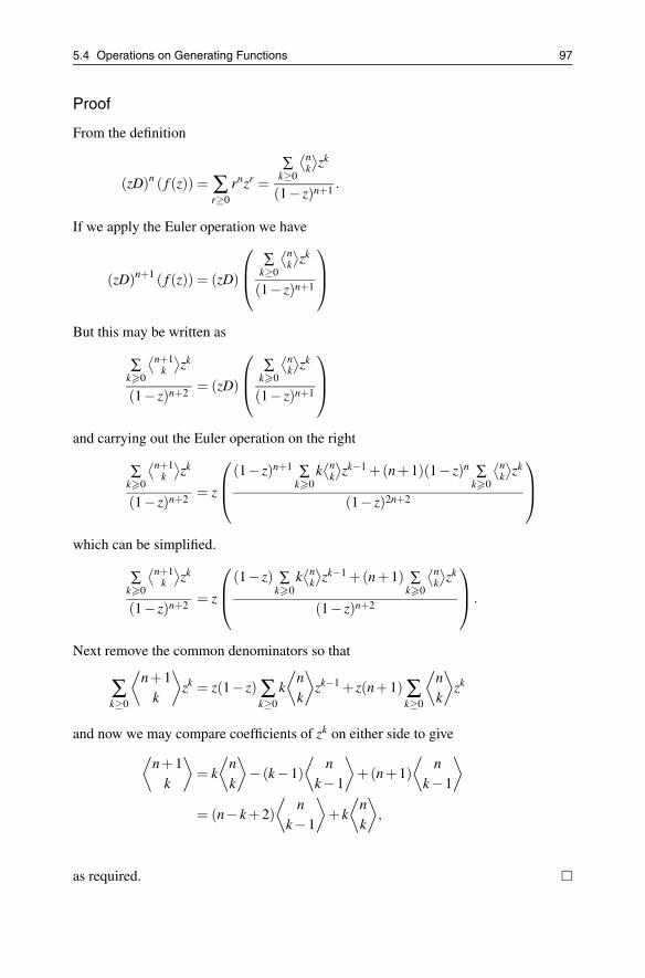
5.4 Operations on Generating Functions 97
Proof
From the definition
(zD)n ( f (z)) = ∑r≥0
rnzr =∑
k≥0
⟨nk
⟩zk
(1− z)n+1 .
If we apply the Euler operation we have
(zD)n+1 ( f (z)) = (zD)
⎛⎜⎝
∑k≥0
⟨nk
⟩zk
(1− z)n+1
⎞⎟⎠
But this may be written as
∑k�0
⟨n+1k
⟩zk
(1− z)n+2 = (zD)
⎛⎜⎝
∑k�0
⟨nk
⟩zk
(1− z)n+1
⎞⎟⎠
and carrying out the Euler operation on the right
∑k�0
⟨n+1k
⟩zk
(1− z)n+2 = z
⎛⎜⎝
(1− z)n+1 ∑k�0
k⟨n
k
⟩zk−1 +(n+1)(1− z)n ∑
k�0
⟨nk
⟩zk
(1− z)2n+2
⎞⎟⎠
which can be simplified.
∑k�0
⟨n+1k
⟩zk
(1− z)n+2 = z
⎛⎜⎝
(1− z) ∑k�0
k⟨n
k
⟩zk−1 +(n+1) ∑
k�0
⟨nk
⟩zk
(1− z)n+2
⎞⎟⎠ .
Next remove the common denominators so that
∑k≥0
⟨n+1
k
⟩zk = z(1− z) ∑
k≥0
k
⟨nk
⟩zk−1 + z(n+1) ∑
k≥0
⟨nk
⟩zk
and now we may compare coefficients of zk on either side to give⟨
n+1k
⟩= k
⟨nk
⟩− (k−1)
⟨n
k−1
⟩+(n+1)
⟨n
k−1
⟩
= (n− k +2)⟨
nk−1
⟩+ k
⟨nk
⟩,
as required.

98 5. Matrices, Sequences and Sums
This recurrence leads directly to an enumerative role for the Eulerian numbers.Rather amazingly, given their origins, they occur in counting the number of ascentsin a permutation.
Definition 5.25 (Ascents in a permutation)
Let π be any permutation of {1,2, . . .r}; an ascent occurs whenever π(i) < π(i+1).
Example 5.26
Given a particular permutation it is easy to count the number of ascents it has. Thepermutation (13)(24) has the bijective form:
(1 3)(2 4) ≡(
1 2 3 43 4 1 2
).
The image of this permutation is (3412) and it has two ascents: 3 ↗ 4 and 1 ↗ 2.
Definition 5.27 (Counting ascents in a permutation)
We denote by ar,k the number of permutations of r objects that have precisely k ascents.
The ascent numbers ar,k make up an array.
Example 5.28
We will find the entries in the row corresponding to r = 3, that is, the distribution ofascents in the permutations of {1,2,3}. First we list them in cycle form (since it iseasy to list them in this form) and then the image of the corresponding bijective form;from the latter we can easily read off the number of ascents (Table 5.1).
We conclude that of the permutations of {1,2,3} there is (are):
(i) 1 permutation with no ascents;
(ii) 4 permutations with a single ascent;
(iii) 1 permutation with two ascents.
So a3.0 = 1, a3,1 = 4, a3,2 = 1 and a3,3 = 0.
These results are very suggestive. We shall prove that the distribution of ascentsin permutations is closely related to the terms of the Eulerian array. We do this byfinding a recurrence they satisfy.
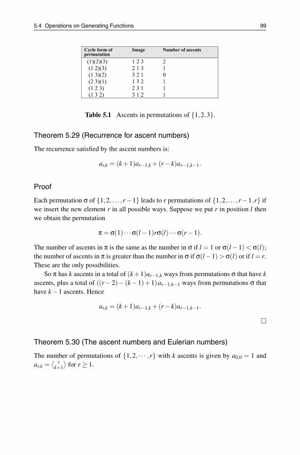
5.4 Operations on Generating Functions 99
Table 5.1 Ascents in permutations of {1,2,3}.
Theorem 5.29 (Recurrence for ascent numbers)
The recurrence satisfied by the ascent numbers is:
ar,k = (k +1)ar−1,k +(r− k)ar−1,k−1.
Proof
Each permutation σ of {1,2, . . . ,r−1} leads to r permutations of {1,2, . . . ,r−1,r} ifwe insert the new element r in all possible ways. Suppose we put r in position l thenwe obtain the permutation
π = σ(1) · · ·σ(l −1)rσ(l) · · ·σ(r−1).
The number of ascents in π is the same as the number in σ if l = 1 or σ(l−1) < σ(l);the number of ascents in π is greater than the number in σ if σ(l−1) > σ(l) or if l = r.These are the only possibilities.
So π has k ascents in a total of (k+1)ar−1,k ways from permutations σ that have kascents, plus a total of ((r−2)− (k−1)+1)ar−1,k−1 ways from permutations σ thathave k−1 ascents. Hence
ar,k = (k +1)ar−1,k +(r− k)ar−1,k−1.
Theorem 5.30 (The ascent numbers and Eulerian numbers)
The number of permutations of {1,2, · · · ,r} with k ascents is given by a0,0 = 1 andar,k =
⟨ rk+1
⟩for r ≥ 1.

100 5. Matrices, Sequences and Sums
Proof
The Eulerian numbers obey the recurrence⟨
rk +1
⟩= (r− k)
⟨r−1
k
⟩+(k +1)
⟨r−1k +1
⟩
which is exactly the same recurrence as that for ar,k. So the Eulerian numbers and theascent numbers ar,k share the same initial values and the same recurrence – they takeidentical values, suitably displaced.
Corollary 5.31 (Properties of Eulerian and ascent numbers)
The Eulerian numbers have the property that
∑k≥0
⟨rk
⟩= r! and
⟨rk
⟩=
⟨r
r− k +1
⟩.
Proof
The first part is an easy consequence of the fact that ∑k≥0 ar,k = r! because they countall the permutations of {1,2, . . . ,r} since any permutation either has no ascents, or 1ascent etc. The second comes from another enumerative insight. There are as manypermutations of r objects with k ascents as there are with k descents. Moreover, if apermutation of r objects has k ascents then it has r− k descents; hence the result.
Rather surprisingly, we can use the Euler operation to obtain sums of powers ofpositive integers.
Example 5.32
We seek a formula for the sum of the first n cubes of the positive integers ∑nk=1 k3. We
need only use the sum operation of Theorem 5.19 on Equation (5.5) when n takes thevalue n = 3. We have
(1
1− z
)∑r≥0
r3zr =(
11− z
) ∑k≥0
⟨3k
⟩zk
(1− z)4 =z+4z2 + z3
(1− z)5 =(z+4z2 + z3) ∑
r≥0
(r +4
4
)zr.
Comparing the coefficients of zn on either side we have
n
∑k=1
k3 =(
n+34
)+4
(n+2
4
)+
(n+1
4
).
5.4 Operations on Generating Functions 101
So
n
∑k=1
k3 =n2(n+1)2
4.
In principle, we have solved the problem of finding the sums of the powers ofthe positive integers for any positive integer power. We simply make use of the corre-sponding row of the Eulerian array. In fact we can extend this further. The correspond-ing result for the alternating sum comes when we apply an additional twist. We startwith a sibling function
∑r≥0
(−1)rzr =1
1+ z;
a first application of the Euler operation gives
∑r≥0
r(−1)rzr =−z
(1+ z)2 ;
using the operation yet again gives,
∑r≥0
r2(−1)rzr = z.−(1+ z)2 + z.2.(1+ z)
(1+ z)4 =−z+ z2
(1+ z)3 .
Repeating the same operation one more time
∑r≥0
r3(−1)rzr = z.(−1+2z)(1+ z)3 − (−z+ z2).3.(1+ z)2
(1+ z)6
=−z+4z2 − z3
(1+ z)4 .
Notice the appearance of the signed Eulerian array – which is easily proved by chang-ing z into −z in the original array. We put this to good use.
Example 5.33
We will find a formula for the alternating sum of the first n cubes of the positive
integersn∑
k=1(−1)kk3. We use the sum operation of Theorem 5.19 on the last result –

102 5. Matrices, Sequences and Sums
with a dash of partial fractions. We have(
11− z
)∑r≥0
r3(−1)rzr =−z+4z2 − z3
(1− z)(1+ z)4
=18
(z3 +13z2 −13z−1
(1+ z)4 +1
1− z
)
=18
((z3 +13z2 −13z−1
)∑r≥0
(−1)r(
r +33
)zr + ∑
r≥0
zr
).
Comparing coefficients of zn we find that
n
∑k=0
(−1)kk3 =(−1)n
((n3
)+13
(n+13
)−13
(n+23
)−
(n+33
)+(−1)n
)8
=(−1)n
8
((−1)n +4n3 +6n2 −1
).
We end this section with an explicit form for the Eulerian numbers which may beadapted to count ascents.
Theorem 5.34 (Explicit form for Eulerian numbers)
The Eulerian numbers are given by⟨n
k
⟩= ∑k
l=0
⟨n+1k−l
⟩(−1)k−1ln.
Proof
We start with the result of using the Euler operation, successively, on the function 11−z
∑r≥0
rnzr =∑
k≥0
⟨nk
⟩zk
(1− z)n+1 .
A rearrangement gives
(1− z)n+1 ∑r≥0
rnzr = ∑k≥0
⟨nk
⟩zk
and using the Binomial Theorem on the left gives
(∑r≥0
(n+1
r
)(−1)rzr
)(∑r≥0
rnzr
)= ∑
k≥0
⟨nk
⟩zk.

5.4 Operations on Generating Functions 103
If we compare coefficients of zk on either side we find that
k
∑l=0
(n+1k− l
)(−1)k−l ln =
⟨nk
⟩
exactly as required.
5.4.5 Exercises
Exercise 5.13
Find a formula for the alternating sum of the first n squares of the naturalnumbers.
Exercise 5.14
Show that the generating function for the sequence {Lr+2} is
∑r≥0
Lr+2zr =3+ z
1− z− z2 .
Use this to show that:
(i)r∑
k=0Lk = Lr+2 −1. (Hint: use the sum formula on the generating function
of the Lucas numbers, together with partial fractions);
(ii)r∑
k=0(−3)kLk+2 = 3(−3)rFr+1. (Hint: divide each side of the generating
function above by 3+ z and use it as a weighted sum)
Exercise 5.15
Show that the generating function for the sequence {Lr+3} is 4+3z1−z−z2 . Hence
show thatr∑
k=02r−kLk = 6.2r − Lr+3. (Hint: use the expression 1 − 2z as a
weighted sum.)
Exercise 5.16
By considering the product of the generating functions 11−z2 and z
1−z−z2 showthat:
(i)r∑
k=0F2k = F2r+1 −1;
(ii)r∑
k=0F2k+1 = F2r+2.
What are the corresponding Lucas results?
104 5. Matrices, Sequences and Sums
5.5 Miscellaneous Exercises
Exercise 5.17
By multiplying suitable generating functions find expressions for ∑rk=0 FkFr−k
and ∑rk=0 LkLr−k. (Hint: see Example 5.18.)
Exercise 5.18
Consider the sequence {ur} in which ur = rFr. Find a recurrence relation satis-fied by the sequence. (Hint: apply the Euler operator to the generating functionof the Fibonacci sequence.)
Exercise 5.19
Show that the generating function for the sequence {Fr+2} is 1+z1−z−z2 and use
this to show that
Fr+1 =r
∑k=0
(−1)r−kFk+2.
Exercise 5.20
Prove that 2Fr+1 =r∑
k=0(Lk −Fk) and 5Fr = Lr+1 +Lr−1.
Exercise 5.21
By applying the Euler operator to a the sum formula for a GP, prove that theformula for the “weighted” sum of a GP is given by
n
∑k=0
kak =(n+1)an
a−1− an+1 −1
(a−1)2 (a = 1).
Exercise 5.22
This question concerns the sum ∑rk=1 k2 = r(r+1)(2r+1)
6 .
(i) Show that k2 =(k
1
)+2
(k2
)and hence use Pascal’s Triangle to show that the
sum takes the value given.
(ii) Now use Eulerian numbers to find the same result.
Exercise 5.23
The Central terms of the even indexed rows of Pascal’s triangle are given by(2rr
). Use an enumerative argument to prove that
(2rr
)= ∑k≥0
(rk
)2.
Exercise 5.24
A new array – like Pascal’s triangle – whose terms are written]r
k
[is defined.
Its first column is the sequence {2,1,1, . . .} and subsequent terms are produced

5.5 Miscellaneous Exercises 105
by the recurrence ]r +1
k
[=
]r
k−1
[+
]rk
[
just like that for Pascal’s triangle. What is the sequence of the diagonal sums?Prove it.
Figure 5.3 Diagonal sums of an array.


6Group Actions and Counting
6.1 The First Steps
In this chapter we count configurations with symmetries, seeking to count only oncethose configurations that are essentially the same. In Chapter 4 we introduced theidea of a group action and the orbits of this action. This is going to be crucial to thedevelopment. Roughly we have an object which we are going to “colour” and we findthe number of ways we can do this if we allow for the symmetries of the object.
Example 6.1
Think of the cube as a dice. We are going to count the number of ways to colour thefaces with the six colours {1,2,3,4,5,6}, insisting that each colour is used. The usualrule is that opposite sides add to seven but there are at least two ways to do this, if youdo not allow reflections (see Figure 6.1). So how many ways can we colour the cubewith six colours using all the colours?
Example 6.2
When we talk about permutations on a set we usually mean a labelled set. That is, wecan distinguish the elements of the set. There are r! permutations if the set has sizer. What happens if the set was unlabelled? Then there is only one permutation, sinceany ordering is the same. What happens if there are four elements and just two labels,
A. Camina, B. Lewis, An Introduction to Enumeration,Springer Undergraduate Mathematics Series,DOI 10.1007/978-0-85729-600-9 6, © Springer-Verlag London Limited 2011
107

108 6. Group Actions and Counting
Figure 6.1 Two dice: different?
say d and e? It is easy to list the possibilities ddee, dede, deed, eedd, eded and edde.Labelling makes a difference: labelling and coloring are the same.
The difficulty in being precise comes from the wide range of objects we wish tocount: they might be geometric, algebraic or something which might not appear to bemathematical. How does this affect the counting? The key point is that we do not wantto count repeats, that is things which appear the same under the group of symmetries.The best way to proceed is to give some examples and then develop the ideas further.
Figure 6.2 A square configuration.
Example 6.3
Let ABCD be a square and assume that the diagonal BD is joined, as in Figure 6.2.

6.1 The First Steps 109
What is the symmetry group, G, of this figure? It is obviously not the whole symmetrygroup of the square, which has order 8. It is not too difficult to see that there are onlyfour symmetries which we will describe by their actions on the vertices: the identity,rotation through π, (AC)(BD), reflection in the axis AC, (BD), and reflection in theaxis BD, (AC). So G has order 4.
What are the orbits of this symmetry group on vertices? It is easy to see thatone orbit is {A, C} and another is {B, D}. Geometrically this is clear, as the verticesA and C have two edges joining them to other vertices, but vertices B and D haveonly three edges joining them to other vertices. Note that G(A) = {A, C} = G(C) andG(B) = {B, D} = G(D). Also we can check that GA = {1,(BD)} so |GA| = 2 and[G : GA] = 2, as required by the Orbit-Stabilizer Theorem 4.48.
We might also look at the action on edges. There are five edges. This time thereare still two orbits: one consists of the outside edges and the other of the diagonal.
Theorem 6.4 (Number of orbits using fixed points)
Let G be a finite group and let G act on X . Let k be the number of orbits then
k =1|G| ∑
g∈G
|Fix(g)|. (6.1)
Proof
By the Orbit-Stabilizer Theorem |Fix(g)| = [G : G(g)]. Let x1, x2, . . . ,xk be chosen sothat each xi is in a different orbit. Now collect the terms on the right-hand side ofequation above according to which orbits they are in:
1|G| ∑
g∈G
|Fix(g)| = 1|G|
k
∑1
|G||G(xi)|
× |G(xi)| = k
as required.
We now have a corollary which we will use later.
Corollary 6.5 (Orbits on pairs)
Let G be a finite group and let G act on X . Let k be the number of orbits of G actingon X ×X . Then
k =1|G| ∑
g∈G
|Fix(g)|2. (6.2)

110 6. Group Actions and Counting
Proof
The action on X ×X is defined by g(x,y) = (gx,gy) for all (x,y) ∈ X ×X . So thenumber of fixed points in this action is just |Fix(g)|2 and hence the result.
We will discuss fixed points further in Section 7.4.
Definition 6.6 (Transitive Group)
Let G be a finite group and let G act on X . If the number of orbits is one then G iscalled transitive, if not it is called intransitive.
Corollary 6.7
Let G be a finite group and let G act on X . If G is transitive then:
1 =1|G| ∑
g∈G
|Fix(g)|.
Example 6.8
Let G be the symmetry group of the “square configuration” of Figure 6.2. Consider Gacting on vertices, the group is given by {1,(AC)(BD), (BD), (AC)} and has order 4.So Equation (6.1) says the number of orbits is given by
4+2+2+04
= 2,
as we already knew.Now consider the action of G on the edges. Then we get
5+1+1+14
= 2,
again as before.
In Example 6.8 we can see a general idea: there is some object which we wish tocolour and the object has a symmetry group which may act on different parts of theobject. For this example it was vertices or edges. In each case the symmetry groupinduces a permutation group on the parts we want to colour. So in our generalizationwe assume that the set we wish to colour comes equipped with a permutation group.However, we do not specify where the permutation group comes from. So in anyparticular application we have to begin by determining the group.
We begin with a counting result at the heart of this development which is a conse-quence of the Orbit-Stabilizer Theorem.

6.1 The First Steps 111
Theorem 6.9 (Number of orbits using stabilizers)
Let G be a finite group and let G act on X . Let k be the number of orbits then
k =1|G| ∑
x∈G
|Gx|. (6.3)
Proof
If x,y are in the same orbit then |Gx)|= |Gy| by the Orbit-Stabilizer Theorem. So eachorbit contributes |Gx|× |G(x)|. But this is just |G|. The result now follows.
6.1.1 Exercises
Exercise 6.1
Let G be a transitive permutation group of degree greater than 1. Prove thatthere is an element in G with no fixed points.
Exercise 6.2
Let G act on X . Further assume that only the identity has fixed points. Provethat |G| divides |X | and that G is transitive if and only if |G| = |X |.
Exercise 6.3
Let H be a regular hexagon with vertices A,B,C,D,E,F labelled clockwise.Join the pairs A,E and B,D. Calculate the symmetry group G of H and countthe number of orbits on vertices and edges.
Exercise 6.4
Let G be the symmetry group of the square. Let G act on X where X is the setof pairs of vertices. Find the number of orbits and their sizes.
Exercise 6.5
Let the cyclic group of order p generated by g act on the set of all p-tuples ofelements from {1,2, . . . ,n} by defining
g(x1,x2, . . . ,xp) = (xp,x1, . . . ,xp−1).
By counting orbits, prove that np ≡ n (mod p).
112 6. Group Actions and Counting
6.2 Colourings and the Cycle Index
Now we come to an important application of the ideas we have developed – given anobject, in how many ways can it be coloured? Clearly the answer will depend on thenumber of colours and the symmetry of the object. We start with a simple version ofthis problem.
Example 6.10
Given a rod and some beads of different colours. How many ways can we constructa rod with two beads on it where we do not mind whether we start from the left orright? Either we have two beads of the same colour or two of different colours. Alsothe number of ways depends on the number of colours. If the number of colours is kthere are k ways with one colour and
(k2
)with two colours. Note that the group is very
simple, just of order 2.
Example 6.11
Now for a slightly more complicated case. Take a triangle with three beads, one ateach vertex. The symmetry group of a triangle, which is just a 3-gon, has order 6.
Either we have three beads the same colour, two the same or all different. No-tice because of the symmetry it doesn’t matter which one is different when only twocolours are used. So the number of ways depends on the number of colours. Let thenumber of colours be k. Then there are k ways with one colour. It is possible to choosetwo colours in
(k2
)ways. But choosing two red and one black, say, is different from
choosing two black and one red. So there are k(k−1) ways to colour the triangle withtwo colours. Finally, with three colours there are just
(k3
)ways.
Note that in these two examples, if we had not been concerned with the symmetriesthe numbers would have been k2 and k3 respectively.
To develop the ideas of colouring we need some ingredients and a recipe.
Definition 6.12 (Colouring)
Given a set X with a group G acting on it, a set of colours (say C) and finally a mapfrom C → X , which is the colouring. The set of all maps, colourings, will be denotedby C . We will assume that X = n and |C| = k.
Lemma 6.13
In the situation given by Definition 6.12, G acts on the set of all colourings C in the

6.2 Colourings and the Cycle Index 113
following way:
if c ∈ C and g ∈ G then g(c)(x) = c(gx) for all x ∈ X .
Then the number of colourings is the number of orbits of G on C .
Proof
To see that this defines an action, we observe that
g(h(c(x)) = g(c(h(x)) = c(gh(x)),
for all g ∈ G, c ∈ C and x ∈ X .To say that two colorings are equivalent is saying that the group action maps one
to the other.
Definition 6.14 (Cycle index)
Let G be a permutation group of degree n. Let X1,X2, . . . ,Xn be n indeterminates. Letg ∈ G and let g have nk cycles of length k. Then the term ∏n
1 Xnkk is called the cycle
symbol, labelled cs(g) of g. Then the cycle index of G is
PG[X1,X2, . . . ,Xn] =∑g∈G cs(g)
|G| .
We often drop the indeterminates and just write PG.
The cycle index can be thought of as a type of generating function. It is interestingto note that we always divide through by the order of G. So all these expressions aretaking an “average”.
Example 6.15
Start with the simplest example, G = Sym(2). Note that the identity element gives Xn1
where n is the degree. The only other element is the transposition (12), which givesX2, one cycle of length two. So
PG =X2
1 +X2
2.
Example 6.16
This time let G be Sym(3). So G has six elements and its degree is 3. The identity ele-ment gives X3
1 , this time a transposition gives X1X2 and the three cycles give X3. Since

114 6. Group Actions and Counting
G has 3 transpositions and 2 three cycles (we get this count from Proposition 2.3),
PG =X3
1 +3X1X2 +2X3
6.
The importance of this idea is evident when we think about the Orbit-StabilizerTheorem. In this we need to know how many things an element fixes. So what happenswhen we fix an element g ∈ G and try to see which colourings it fixes? If g fixes acolouring and two elements of X are in the same cycle of g they must share the samecolour. Since each cycle is independent of every other cycle we can colour each cycleindependently. If there are m cycles altogether and k colours there are km ways thiscan be done. This is the value of cs(g) with each indeterminate replaced by k.
Proposition 6.17
Let G act on X and let C be a the set of colourings from a set of colours C, |C|= k. Letcm be the number of elements of G with exactly m cycles. Then the number of orbitsof G on C is given by:
∑∞1 cmkm
|G| .
Proof
This now follows immediately from Theorem 6.4.
Example 6.18
In Example 6.15 we can put Xi = k, i = 1,2 and get
P(k,k) =k2 + k
2.
In Example 6.10 we counted k colourings with one colour used and(k
2
)colourings
when both colours were used. We note that
k +(
k2
)=
k2 + k2
.
Example 6.19
In Example 6.16 we can put Xi = k for each i and get
P(k,k) =k3 +3k2 +2k
6.
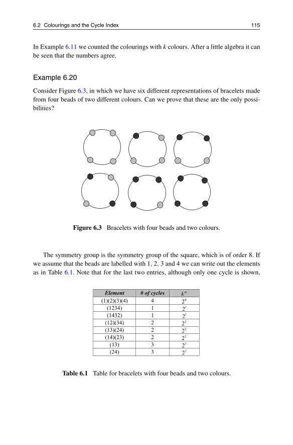
6.2 Colourings and the Cycle Index 115
In Example 6.11 we counted the colourings with k colours. After a little algebra it canbe seen that the numbers agree.
Example 6.20
Consider Figure 6.3, in which we have six different representations of bracelets madefrom four beads of two different colours. Can we prove that these are the only possi-bilities?
Figure 6.3 Bracelets with four beads and two colours.
The symmetry group is the symmetry group of the square, which is of order 8. Ifwe assume that the beads are labelled with 1, 2, 3 and 4 we can write out the elementsas in Table 6.1. Note that for the last two entries, although only one cycle is shown,
Table 6.1 Table for bracelets with four beads and two colours.

116 6. Group Actions and Counting
there are two fixed points which give 2 one cycles. Now
PG(2,2,2,2) =24 +2.21 +3.22 +2.23
8= 6.
We get 6 as we anticipated, confirming that these are the only possibilities.
Example 6.21
If we consider the previous example it is easy to see what happens if there are threecolours as in the following table:
Table 6.2 Table for bracelets with three colours.
Now
PG(3,3,3,3) =34 +2.31 +3.32 +2.33
8= 21.
All these examples show that this only goes so far – it calculates the total numberof colourings but does not detail how many there are with further restrictions. Forexample we might want to know how many have exactly two white beads and howmany with two black beads. This is our next task.
6.2.1 Exercises
Exercise 6.6
In how many ways can we paint the faces of a cube using two colours if weallow only rotations of the cube?
Exercise 6.7
Calculate the cycle index of the group Alt(4).

6.3 Polya’s Theorem 117
Exercise 6.8
Consider the situation in Exercise 6.3. Calculate the cycle index of the symme-try group. Then calculate how many colourings, with k colours, there are of thevertices.
Exercise 6.9
In Exercise 4.14 we calculated the symmetry group of the tetrahedron. Nowcalculate the cycle index of the symmetry group. Show that with two and threecolours, respectively, there are 5 and 15 colourings of the vertices and facesand 11 and 66 colourings of the edges.
Exercise 6.10
Consider the square and the action of the symmetry group on pairs of vertices,as in Exercise 6.4. Find the cycle index for this action.
6.3 Polya’s Theorem
We begin this section by defining an expression that counts the number of colouringswith different configurations.
Definition 6.22 (Colouring inventory)
Given a colouring with C = {c1,c2, . . . ,ck} the set of colours and G acting on X . LetC be the set of all possible colourings.
The colouring inventory of a subset D ⊂ C is a polynomial in {c1,c2, . . . ,ck}which is the sum of terms of the form ∏cdi
i with coefficients which count how manycolourings there are in D with di elements of X coloured ci.
Example 6.23
Let us reconsider Example 6.20. First consider all the possible bracelets, and use C ={b,w}. We will calculate the colouring inventory polynomial by exhaustion, that iswe will list all the possibilities. Those which have exactly one colour will be the termsb4 and w4; with two colours, one occurring three times gives 4wb3 and 4bw3, sincethere are four choices to allocate the single colour; finally, there are six possibilitiesfor two colours each occurring twice, since we can choose any two positions for thetwo colours, giving 6b2w2. Notice in this count we do not look at the action of thegroup. So the colouring inventory polynomial is
b4 +4b3w+6b2w2 +4bw3 +w4 = (b+w)4.

118 6. Group Actions and Counting
We could look at the subset fixed by a permutation, say g = (1,3). This will fixthose colourings which have a particular diagonal pair the same colour, assuming thelabelling was clockwise. So the corresponding colouring inventory polynomial will be
b4 +3b3w+4b2w2 +3bw3 +w4.
Definition 6.24 (Pattern inventory)
Given a colouring with G acting on X , with C = {c1,c2, . . . ,ck}, the set of colours. LetC be the set of all possible colourings. The pattern inventory of a subset D ⊂ C is apolynomial in {c1,c2, . . . ,ck} which is the sum of terms of the form ∏cdi
i with coeffi-cients which count how many equivalent colourings there are in D with di elementsof X coloured ci.
The important point here is that the pattern inventory takes account of the group action.
Example 6.25
Let us reconsider, yet again, Example 6.20. Consider all the possible bracelets, usingagain the principle of exhaustion, with C = {b,w}. The pattern inventory will be givenby
b4 +b3w+2b2w2 +bw3 +w4.
Now the question is “How do we find this without enumerating all possibilities?”.
Recall that by Theorem 6.4 the number of orbits depends on the size of the fixed setsof the elements of the group. Here is a key lemma.
Lemma 6.26
Let C = {c1,c2, . . . ,ck} be a set of colours with G acting on X . Let g ∈ G then thecolouring inventory for the set Fix(g) is given by finding the cycle index for g, cs(g)and substituting ∑cr
j for Xr.
Proof
Consider one cycle, say (a1a2 . . .ar) of g. Then if g fixes a colouring then each ofa1,a2, . . . ,ar has to have the same colour. So the pattern inventory for this cycle willbe cr
1 +cr2 + · · ·+cr
k. In cs(g) this cycle contributes the term Xr. For each cycle we cando the same, and as each cycle is disjoint, the choices for each cycle can be multiplied

6.3 Polya’s Theorem 119
together. So the total number of colourings fixed by g is the product
∏each cycle
cr1 + cr
2 + · · ·+ crk.
This is the same as the value of cs(g) with each indeterminate Xr replaced by cr1 +cr
2 +· · ·+ cr
k. The lemma follows.
Theorem 6.27 (Polya’s Theorem)
Let C = {c1,c2, . . . ,ck} be a set of colours with G acting on X . Then the pattern in-ventory is given by substituting ∑cr
j for Xr. Thus the pattern inventory is
PG
(∑c j,∑c2
j , . . . ,∑ckj
).
Proof
We use the result of Theorem 6.4. For any particular colouring, to find the number ofequivalence classes, we add the numbers of fixed points and divide by the order of G.But by the previous lemma the inventory for Fixg is just cs(g) with the appropriatesubstitution and the average is just the definition of PG.
Example 6.28
Once more we reconsider Example 6.20. First we need to calculate PG, which is quitestraightforward:
PG =18
(X4
1 +2X21 X2 +3X2
2 +2X4).
For two colours {b,w} the pattern inventory is
18
((b+w)4 +2(b+w)2(b2 +w2)+3(b2 +w2)2 +2(b4 +w4)
).
After some expansion we get b4 + b3w + 2b2w2 + bw3 + w4, which is precisely thesame result we established earlier by direct enumeration.
Example 6.29
We will count the number of ways we can colour a square board with black and whitesquares. We can count this using Polya’s Theorem 6.27. We need to calculate thecyclic index polynomial for the symmetry group acting on the board. This is a groupof order 8, the symmetry group of the square. In this example we will only consider
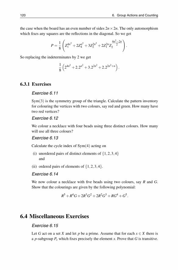
120 6. Group Actions and Counting
the case when the board has an even number of sides 2n×2n. The only automorphismwhich fixes any squares are the reflections in the diagonal. So we get
P =18
(Z4n2
1 +2Zn2
4 +3Z2n2
2 +2Z2n1 Z
4n2−2n2
2
).
So replacing the indeterminates by 2 we get
18
(24n2
+2.2n2+3.22n2
+2.22n2+n)
.
6.3.1 Exercises
Exercise 6.11
Sym(3) is the symmetry group of the triangle. Calculate the pattern inventoryfor colouring the vertices with two colours, say red and green. How many havetwo red vertices?
Exercise 6.12
We colour a necklace with four beads using three distinct colours. How manywill use all three colours?
Exercise 6.13
Calculate the cycle index of Sym(4) acting on
(i) unordered pairs of distinct elements of {1,2,3,4}and
(ii) ordered pairs of elements of {1,2,3,4}.
Exercise 6.14
We now colour a necklace with five beads using two colours, say R and G.Show that the colourings are given by the following polynomial:
R5 +R4G+2R3G2 +2R2G3 +RG4 +G5.
6.4 Miscellaneous Exercises
Exercise 6.15
Let G act on a set X and let p be a prime. Assume that for each x ∈ X there isa p-subgroup Px which fixes precisely the element x. Prove that G is transitive.
6.4 Miscellaneous Exercises 121
Exercise 6.16
Let C be a cyclic group of order p, for some prime p. Consider the regularaction of C on itself. Prove:
PC(X1,X2, . . . ,Xp) =1p
(X p
1 +(p−1)Xp).
Hence show that kp ≡ k (mod p) for any k ∈ N.
Exercise 6.17
Let G be the group of rotational symmetries of the cube. Calculate the cycleindex for G acting on the faces. Then calculate the pattern inventory for colour-ing the faces with red, white and blue. Show that there are six different ways touse both colours twice.
Exercise 6.18
This final exercise is an application to music. In twelve tone rows the musicianis allowed to choose a row of distinct notes from the twelve tone scale. Tworows are considered the same if they can be transformed by transposing orinverting. The question is, given a row of say six notes, how many rows arewe allowed? This can be translated as follows. The possible notes, called pitchclasses, are labelled from 0 to 11, so we think of them as the integers mod 12.The twelve transformations are called Tn : x → x + n (mod 12) and TnI : x →−x+n (mod 12). Show that the numbers in the table below are correct.


7Exponential Generating Functions
7.1 Another Generating Function
It is not clear why another generating function is needed, but it turns out that whenwe count the number of permutations of different types, these are the natural gener-ating function. We can see this by looking at a simple enumeration: the number ofpermutations of r things.
Example 7.1
We will attempt to find the generating function of the sequence {ur} = {r!}. Writtenas a power series, the generating function is
F(z) = 1+1z+2z2 +6z3 +24z4 + · · · .
And that is as far as we can go. There is nothing simple we can do with this to find afunction whose expansion this is. But that isn’t the only problem. The ratio test tellsus that such a function has a zero radius of convergence: it converges only when z = 0.Despite this, we can still extract enumerative information from it, but not with thebenefit of an analytic function in some of the ways we have done hitherto.
Definition 7.2 (Exponential generating function egf )
Given any sequence {ur} = {u0,u1,u2, . . .} the exponential generating function (egf )
A. Camina, B. Lewis, An Introduction to Enumeration,Springer Undergraduate Mathematics Series,DOI 10.1007/978-0-85729-600-9 7, © Springer-Verlag London Limited 2011
123

124 7. Exponential Generating Functions
of the sequence is the function U(z) in which
U(z) =u0
0!+
u1z1!
+u2z2
2!+ · · · = ∑
r≥0
urzr
r!.
Note: we refer to the generating function
U(z) = ∑r≥0
urzr
as the ordinary generating function (ogf ) of the sequence. This definition solves theproblem of finding a generating function for permutations.
Example 7.3
The exponential generating function (egf ) of the sequence, {ur} = {r!} is given by
Ueg f (z) = ∑r≥0
urzr
r!= ∑
r≥0
r!zr
r!= ∑
r≥0
zr =1
1− z,
which has radius of convergence |z| < 1.
Example 7.4
It is useful to see the difference between an ordinary generating function (ogf ) and thecorresponding exponential generating function (egf ) of a particular sequence; we takethe simple sequence {ur} = {1,1,1, . . .}. We have:
(i) the ogf is Uogf(z) = ∑r≥0
urzr = ∑r≥0
zr = 11−z ;
(ii) the egf is Uegf(z) = ∑r≥0
urzr
r! = ∑r≥0
zr
r! = ez.
There is an important enumerative difference between the two types of generatingfunction. Here is a cautionary but illuminating example that highlights the difference.
Example 7.5
We find the number of ways that three letters, chosen from the letters of SEQUENCE,can be arranged. The ordinary generating function for the choice of the three possibleEs is 1 + z + z2 + z3; that for each of the letters C, N, S, Q and U is 1 + z. So thegenerating function is
(1+ z)5(1+ z+ z2 + z3)

7.1 Another Generating Function 125
and the answer we seek is the coefficient of z3, which is
1+5.1+10.1+10.1 = 26.
But what we have calculated is the number of non-negative integer solutions of theequation s+ e+q+u+n+ c = 3, in which 0 ≤ e ≤ 3 and 0 ≤ s,q,u,n,c ≤ 1. This isnot the answer. A selection of three letters from SEQUENCE has (by the principle ofexhaustion) either none, one or two Es (Table 7.1) and so:
Table 7.1 Arranging the letters of SEQUENCE.
The distinction that needs to be made is between:
(i) making a selection;
(ii) making a selection and then arranging (or if you prefer, labelling) those selected.
We obtain the count of the number of “words” from an egf. The exponential generatingfunction for the letter E is
1+z1!
+z2
2!+
z3
3!;
that for each of the letters C, N, S, Q and U is
1+z1!
= 1+ z.
So the required egf is
(1+ z)5(
1+z1!
+z2
2!+
z3
3!
).
We seek the coefficient of z3
3! and this is 1+5.1.3+10.1.6+10.6 = 136.
We explore some some particular sequences and their egf s.
126 7. Exponential Generating Functions
Example 7.6
We find the egf of the sequence {ur}= {r2}. We may write r2 = r(r−1)+ r and then
∑r≥0
urzr
r!= ∑
r≥0
r2zr
r!
= ∑r≥0
(r(r−1)+ r)zr
r!= ∑
r≥2
zr
(r−2)!+ ∑
r≥1
zr
(r−1)!
= z2 ∑r≥2
zr−2
(r−2)!+ z ∑
r≥1
zr−1
(r−1)!= z2ez + zez
=(z2 + z
)ez.
Theorem 7.7 (egf of Fibonacci and Lucas sequences)
The egf for the Fibonacci and Lucas sequences are
(i) ∑r≥0
Frzr
r! = 1√5
(eφ1z − eφ2z
);
(ii) ∑r≥0
Lrzr
r! =eφ1z + eφ2z.
Proof
We start with Binet’s formula
∑r≥0
Frzr
r!= ∑
r≥0
1√5
(φr1 −φr
2)zr
r!
=1√5
(∑r≥0
(φ1z)r
r!− ∑
r≥0
(φ2z)r
r!
)
=1√5
(eφ1z − eφ2z) .
The proof for the Lucas numbers is in the exercises.
7.1.1 Exercises
Exercise 7.1
In how many ways can four letters chosen from the letters of FUNCTION bearranged?

7.2 Recurrence to egf 127
Exercise 7.2
Find the egf of the sequence whose terms consist of:
(i) the Lucas numbers Lr (this completes the proof of Theorem 7.7);
(ii) the even indexed Fibonacci numbers, F2r.
Exercise 7.3
Consider the sequence {ur} in which ur = r3. By writing the terms of the se-quence in the form
ur = r3 = Ar(r−1)(r−2)+Br(r−1)+Cr
for suitable constants, A, B and C, find the egf of the sequence.
7.2 Recurrence to egf
The basic procedure for converting a recurrence into an exponential generating func-tion does not differ from the corresponding procedure for an ordinary generating func-tion – the three-step recipe (Algorithm 2.23). Of course, we need to introduce thefactorial term as part of the summation. We illustrate it with a sequence we have en-countered on more than one occasion: the derangement sequence.
Example 7.8 (The derangement sequence)
We will use two recurrences that we have for this sequence: Example 2.19 and itsequivalent from Exercise 2.8.
(i) The first step is to write out the recurrence
dr+1 = r(dr +dr−1) (noting that d0 = 1, d1 = 0.)
(ii) The next step is quite straightforward (remember the new factorial element):
∑r≥1
dr+1zr
r!= ∑
r≥1
rdrzr
r!+ ∑
r≥1
rdr−1zr
r!.
(iii) Suppose the egf required is D(z) then
D′(z)−d1 = z ∑r≥1
drzr−1
(r−1)!+ z ∑
r≥1
dr−1zr−1
(r−1)!
D′(z) = zD′(z)+ zD(z).
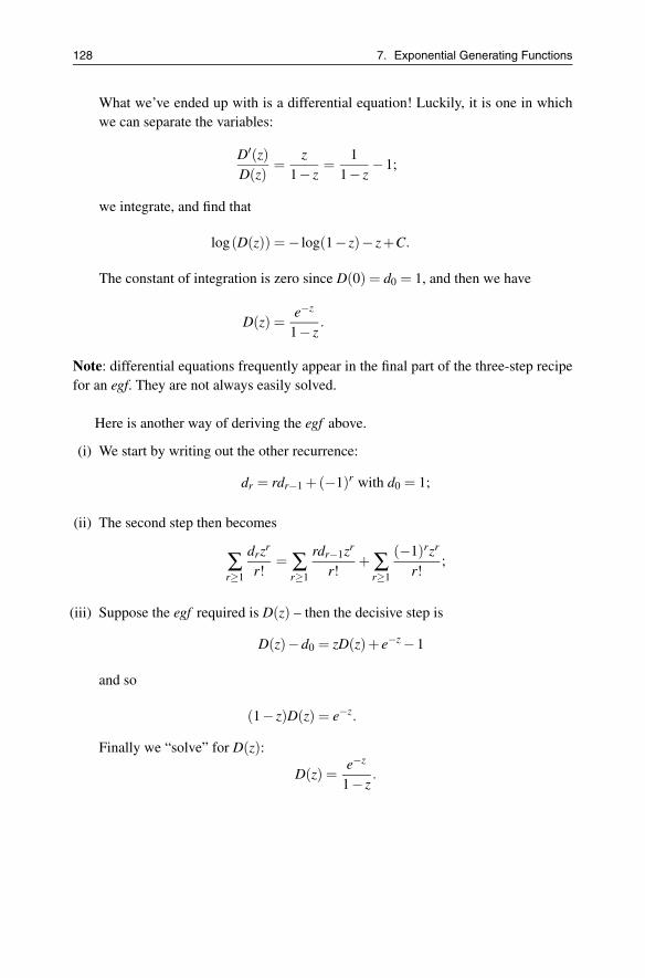
128 7. Exponential Generating Functions
What we’ve ended up with is a differential equation! Luckily, it is one in whichwe can separate the variables:
D′(z)D(z)
=z
1− z=
11− z
−1;
we integrate, and find that
log(D(z)) = − log(1− z)− z+C.
The constant of integration is zero since D(0) = d0 = 1, and then we have
D(z) =e−z
1− z.
Note: differential equations frequently appear in the final part of the three-step recipefor an egf. They are not always easily solved.
Here is another way of deriving the egf above.
(i) We start by writing out the other recurrence:
dr = rdr−1 +(−1)r with d0 = 1;
(ii) The second step then becomes
∑r≥1
drzr
r!= ∑
r≥1
rdr−1zr
r!+ ∑
r≥1
(−1)rzr
r!;
(iii) Suppose the egf required is D(z) – then the decisive step is
D(z)−d0 = zD(z)+ e−z −1
and so
(1− z)D(z) = e−z.
Finally we “solve” for D(z):
D(z) =e−z
1− z.
7.3 Operations on egfs 129
7.2.1 Exercises
Exercise 7.4
Attempt to convert the recurrence tr+2 = tr+1 +(r+1)tr with t0 = t1 = 1 into anegf. Now write it in the form tr+1 = tr + rtr−1 and repeat the process. (Moral:you sometimes have to be creative.)
Exercise 7.5
The push-button lock sequence {cr} obeys the recurrence cr = rcr−1 + 1 (Ex-ercise 5.6). Use this to find its egf.
7.3 Operations on egfs
We can do all the things with an egf that we can do with an ogf ; we often do them indifferent ways though. We start with the operations that we can perform on egf s. Thisagain helps with the final step in the three-step recipe of converting a recurrence intoa generating function – now adapted to exponential generating functions. It providesa repertoire of techniques that we can exploit, just as before. Many of the operationswe have already encountered for ogf s apply to egf s and these are not repeated. Othersare adapted to a new purpose. Some have restricted use in this new environment: thesum operator is one such example.
7.3.1 Differentiation
If we differentiate the exponential generating function
U(z) = ∑r≥0
ur
zr r!,
we find that
U ′(z) = ∑r≥1
rurzr−1
r!= ∑
r≥1
urzr−1
(r−1)!;
we may re-index this sum r−1 → r so that,
U ′(z) = D(U(z)) = ∑r≥0
ur+1zr
r!.
This proves an important result.

130 7. Exponential Generating Functions
Theorem 7.9 (Derivative of an egf )
The derivative of the egf of a sequence {ur} is the egf for the sequence {ur+1}.
This operation is frequently used to derive recurrence relations.
Example 7.10
By differentiating the egf of the push-button lock sequence {cr}, which has the egfez
1−z (and using the previous theorem), we find that
∑r≥0
cr+1zr
r!=
(1− z)ez + ez
(1− z)2 =ez
1− z+
11− z
(ez
1− z
)
= ∑r≥0
crzr
r!+
11− z ∑
r≥0
crzr
r!
and then we have
(1− z) ∑r≥0
cr+1zr
r!= (1− z) ∑
r≥0
crzr
r!+ ∑
r≥0
crzr
r!.
If we compare coefficients of zr on either side this gives
cr+1
r!− cr
(r−1)!=
cr
r!− cr−1
(r−1)!+
cr
r!
and then multiplication throughout by r! gives
cr+1 − rcr = cr − rcr−1 + cr
and finally, the recurrence
cr+1 = (r +2)cr − rcr−1.
Notice that this recurrence is not the one you used to derive the egf for this sequencein Exercise 7.5, but we can easily derive it from the latter recurrence.
Example 7.11
We start with the recurrencecr = rcr−1 +1
and hence (increasing the index by 1)
cr+1 = (r +1)cr +1;
if these are subtracted and simplified, we find that
cr+1 = (r +2)cr − rcr−1.

7.3 Operations on egfs 131
7.3.2 Products of Exponential Generating Functions
The result for the product of two egf s (or the square of one) has an unexpected newelement.
Theorem 7.12 (Product formula for two egfs)
In the product of two exponential generating functions W (z) = U(z)V (z), which arethe egf s of the respective sequences {wr},{ur} and {vr}, we have
wr = ∑k≥0
(rk
)ukvr−k.
Proof
We have:
U(z)V (z) =
(∑r≥0
urzr
r!
)(∑r≥0
vrzr
r!
).
This product is itself a generating function W (z) for the sequence {wr} in which:
∑r≥0
wrzr
r!=
(∑r≥0
urzr
r!
)(∑r≥0
vrzr
r!
)
and comparing coefficients of zr on either side gives
wr
r!=
r
∑k=0
ukvr−k
k!(r− k)!
which on multiplication throughout by r! gives the required result.
This product formula, and its predecessor, the product formula for ogf s, providethe means to describe the enumerative difference between the two generating func-tions:
(i) an ogf counts objects of size r which are are obtained by bringing together objectsof size k and r− k in all possible ways;
(ii) an egf counts objects of size r where we not only bring together two objects in theway above, but we also relabel the objects. There are
(rk
)ways to choose the new
labels of the elements of the object ak (or indeed br−k because of the symmetryof Binomial coefficients).
The product formula is a very practical result and it is often used to derive egf swithout recourse to the three-step recipe.
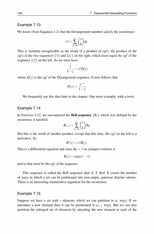
132 7. Exponential Generating Functions
Example 7.13
We know (from Equation 1.2) that the Derangement numbers satisfy the recurrence:
r! =r
∑k=0
(rk
)dk.
This is instantly recognisable as the result of a product of egf s, the product of theegf s of the two sequences {1} and {dr} on the right, which must equal the egf of thesequence {r!} on the left. So we must have
11− z
= ezD(z)
where D(z) is the egf of the Derangement sequence. It now follows that
D(z) =e−z
1− z.
We frequently use this idea later in the chapter. One more example, with a twist.
Example 7.14
In Exercise 5.12, we encountered the Bell sequence {Br} which was defined by therecurrence it satisfied:
Br+1 =r
∑k=0
(rk
)Bk.
But this is the result of another product, except that this time, the egf on the left is aderivative. So
B′(z) = ezB(z).
This is a differential equation and since B0 = 1 its (unique) solution is
B(z) = exp(ez −1)
and so that must be the egf of the sequence.
This sequence is called the Bell sequence after E. T. Bell. It counts the numberof ways in which a set can be partitioned into non-empty, pairwise disjoint subsets.There is an interesting enumerative argument for the recurrence.
Example 7.15
Suppose we have a set with r elements which we can partition in ur ways. If weintroduce a new element then it can be partitioned in ur+1 ways. But we can alsopartition the enlarged set of elements by attaching the new element to each of the

7.3 Operations on egfs 133
ur partitioned subsets. By the principle of exhaustion, the new element is either in asubset by itself or in a subset with one other element or with a subset with two otherelements, and so on. If the subset to which the new element is adjoined has k elementsthen there are
(rk
)ur−k ways to do this (select k, partition the remainder). Hence
ur+1 = ∑k≥0
(rk
)ur−k = ∑
k≥0
(rk
)uk
since the Binomial coefficients are symmetric.
The number of partitions of a set with 1 element is 1, and hence Br = ur because theyshare the same recurrence and initial values. So the Bell numbers enumerate the non-empty, pairwise disjoint partitions of a set into subsets. From Exercise 5.12 we knowthat
{Br} = {1,1,2,5,15,52, . . .}.
Next we look at products of egf s as a way to derive identities.
Example 7.16
We consider the product of ez and L(z) (the egf of the Lucas sequence) and use it toderive an identity. We look at the product in two different ways:
(i) ezL(z) = ez(eφ1z + eφ2z
)= e(φ1+1)z + e(φ2+1)z
and since φi +1 = φ2i , i = 1,2 (Exercise 3.16) we then have
ezL(z) = eφ21z + eφ2
2z = ∑r≥0
(φ2r
1 +φ2r2
)zr
r!= ∑
r≥0
L2rzr
r!;
(ii) but we also have
ezL(z) =
(∑r≥0
zr
r!
)(∑r≥0
Lrzr
r!
).
Using the product theorem (Theorem 7.12) now gives the required identity
L2r = ∑k≥0
(rk
)Lk.
7.3.3 Expanding egfs
An egf can be expanded just as their ogf counterparts are expanded – exactly the sametechniques are employed. When we do this for the Bell sequence we find a surprisingsum for each of its terms.

134 7. Exponential Generating Functions
Example 7.17
The Bell sequence {Br} has egf
∑r≥0
Brzr
r!= exp(ez −1) .
We may rearrange this to get
∑r≥0
Brzr
r!= exp(ez −1) = e−1 exp(ez) = e−1 ∑
s≥0
ezs
s!= e−1 ∑
s≥0
1s! ∑
r≥0
zrsr
r!
and hence
∑r≥0
Brzr
r!= e−1 ∑
r≥0
(∑s≥0
sr
s!
)zr
r!.
The reversal of the infinite sums is justified since each of the sums is absolutely con-vergent. If we now compare coefficients of zr on either side we have,
Br = e−1 ∑s≥0
sr
s!= e−1
(1r
1!+
2r
2!+
3r
3!+ · · ·
).
This is the explicit form for the terms of the sequence – in the form of a convergentinfinite sum. This sum is called Dobinsky’s formula.
7.3.4 Exercises
Exercise 7.6
The derangement sequence {dr} has the egf e−z
1−z . By regarding the right-handside as the product of two egf s and using the product formula (Theorem 7.12),find an explicit form for the derangement numbers. (We derived this enumera-tively in Example 1.27.)
Exercise 7.7
The sequence {tr} has the egf ∑r≥0trzr
r! = ez+ z2
2 . Show that
2r+1
∑k=0
(−1)k+1(
2r +1k
)tk = 0
and find the corresponding result for even r. (The sequence {tr} counts thenumber of permutations that have only cycles of length 1 or 2. Such permuta-tions are called involutions. We shall look at them in detail later in the chapter.)
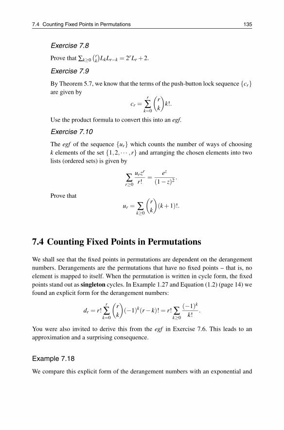
7.4 Counting Fixed Points in Permutations 135
Exercise 7.8
Prove that ∑k≥0
(rk
)LkLr−k = 2rLr +2.
Exercise 7.9
By Theorem 5.7, we know that the terms of the push-button lock sequence {cr}are given by
cr =r
∑k=0
(rk
)k!.
Use the product formula to convert this into an egf.
Exercise 7.10
The egf of the sequence {ur} which counts the number of ways of choosingk elements of the set {1,2, · · · ,r} and arranging the chosen elements into twolists (ordered sets) is given by
∑r≥0
urzr
r!=
ez
(1− z)2 .
Prove that
ur = ∑k≥0
(rk
)(k +1)!.
7.4 Counting Fixed Points in Permutations
We shall see that the fixed points in permutations are dependent on the derangementnumbers. Derangements are the permutations that have no fixed points – that is, noelement is mapped to itself. When the permutation is written in cycle form, the fixedpoints stand out as singleton cycles. In Example 1.27 and Equation (1.2) (page 14) wefound an explicit form for the derangement numbers:
dr = r!r
∑k=0
(rk
)(−1)k(r− k)! = r! ∑
k≥0
(−1)k
k!.
You were also invited to derive this from the egf in Exercise 7.6. This leads to anapproximation and a surprising consequence.
Example 7.18
We compare this explicit form of the derangement numbers with an exponential and

136 7. Exponential Generating Functions
derive another form for them. We have
dr = r!r
∑k=0
(−1)k
k!= r!
(∞
∑k=0
(−1)k
k!−
∞
∑k=r+1
(−1)k
k!
)
= r!e−1 − r!∞
∑k=r+1
(−1)k
k!.
The final term on the right depends on r, and we denote it Rr. It takes the value
Rr = r!∞
∑k=r+1
(−1)k
k!=
(−1)r+1
r +1+
(−1)r+2
(r +1)(r +2)+ · · ·
= (−1)r+1(
1r +1
− 1(r +1)(r +2)
+1
(r +1)(r +2)(r +3)−·· ·
).
More importantly, the size of Rr is such that
|Rr| <(
1r +1
+1
(r +1)2 +1
(r +1)3 + · · ·)
=1r.
So we now have
dr =r!e− (−1)r+1Rr =
r!e
+(−1)rRr
and since, |Rr| < 1r , we have the approximation
dr ≈r!e
which is accurate to the nearest positive integer.
We now collect together the results for derangement numbers.
Theorem 7.19 (The derangement numbers)
The derangement numbers {dr} are such that:
(i) they obey the recurrences
dr = r (dr−1 +dr−2) , dr = rdr−1 +(−1)r and r! = ∑k≥0
(rk
)dk;
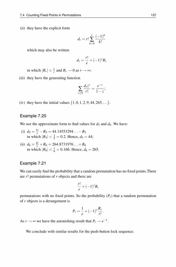
7.4 Counting Fixed Points in Permutations 137
(ii) they have the explicit form
dr = r!r
∑k=0
(−1)k
k!
which may also be written
dr =r!e
+(−1)rRr
in which |Rr| < 1r and Rr → 0 as r → ∞;
(iii) they have the generating function
∑r≥0
drzr
r!=
e−z
1− z;
(iv) they have the initial values {1,0,1,2,9,44,265, . . .}.
Example 7.20
We use the approximate form to find values for d5 and d6. We have:
(i) d5 = 5!e −R5 = 44.14553294 . . .−R5
in which |R5| < 15 = 0.2. Hence, d5 = 44;
(ii) d6 = 6!e +R6 = 264.8731976 . . .+R6
in which |R6| < 16 = 0.166̇. Hence, d6 = 265.
Example 7.21
We can easily find the probability that a random permutation has no fixed points.Thereare r! permutations of r objects and there are
r!e
+(−1)rRr
permutations with no fixed points. So the probability (Pr) that a random permutationof r objects is a derangement is
Pr =1e
+(−1)r Rr
r!.
As r → ∞ we have the astonishing result that Pr → e−1.
We conclude with similar results for the push-button lock sequence.

138 7. Exponential Generating Functions
Theorem 7.22 (The push-button lock sequence)
The push-button lock combinations {cr} are such that
(i) they obey the recurrences
cr = rcr−1 +1,cr = (r +1)cr−1 − (r−1)cr−2 and r! =r∑
k=0(−1)r−k
(rk
)ck;
(ii) they have the explicit form
cr =r
∑k=0
(rk
)k!;
(iii) they have the egf
∑r�0
crzr
r!=
ez
1− z.
Proof
These have all been given in examples or as an exercise:
(i) Exercises 5.6, 5.7 and 5.8;
(ii) Theorem 5.7;
(iii) Exercise 7.5.
We now investigate the distribution of fixed points in permutations. We begin withthe notation used to count the number of permutations (of r objects) that have a givennumber of fixed points.
Definition 7.23 (Number of permutations with precisely k fixed points)
The number dr,k counts the number of permutations of r objects with precisely k fixedpoints.
Note: a permutation with no fixed points is a derangement and so with this notationwe have two (equivalent) ways of writing the same thing: dr,0 ≡ dr.
Theorem 7.24
The explicit form for dr,k is given in terms of derangement numbers dr,k =(r
k
)dr−k.

7.4 Counting Fixed Points in Permutations 139
Proof
A permutation with precisely k fixed points may be constructed as in Figure 7.1.
Figure 7.1 Permutations with precisely k fixed points.
Example 7.25
Using this result we may find the distribution of fixed points in the permutations offour objects. There are, by the previous theorem
(i) d4,4 =(4
4
)d0 = 1.1 = 1 permutation with four fixed points;
(ii) d4,3 =(4
3
)d1 = 4.0 = 0 permutations with three fixed points (if it has three fixed
points, then it must have four – this is where the “precisely” comes in);
(iii) d4,2 =(4
2
)d2 = 6.1 = 6 permutations with two fixed points;
(iv) d4,1 =(4
1
)d3 = 4.2 = 8 permutations with one fixed point;
(v) finally, there are d4 ≡ d4,0 =(4
0
)d4 = d4 = 4!− 1− 0− 6− 8 = 9 permutations
with no (= 0) fixed points.
For a given value of r we have a corresponding set of enumerators dr,k, one foreach value of k. We can arrange these enumerators into an array. We call the array theFixed point matrix.
Definition 7.26 (The Fixed point matrix)
The Fixed point matrix is the array S = (dr,k).
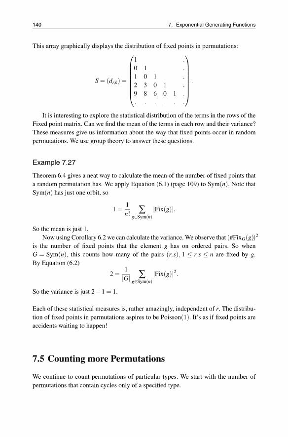
140 7. Exponential Generating Functions
This array graphically displays the distribution of fixed points in permutations:
S = (dr,k) =
⎛⎜⎜⎜⎜⎜⎜⎜⎝
1 .
0 1 .
1 0 1 .
2 3 0 1 .
9 8 6 0 1 .
. . . . . .
⎞⎟⎟⎟⎟⎟⎟⎟⎠
.
It is interesting to explore the statistical distribution of the terms in the rows of theFixed point matrix. Can we find the mean of the terms in each row and their variance?These measures give us information about the way that fixed points occur in randompermutations. We use group theory to answer these questions.
Example 7.27
Theorem 6.4 gives a neat way to calculate the mean of the number of fixed points thata random permutation has. We apply Equation (6.1) (page 109) to Sym(n). Note thatSym(n) has just one orbit, so
1 =1n! ∑
g∈Sym(n)|Fix(g)|.
So the mean is just 1.Now using Corollary 6.2 we can calculate the variance. We observe that (#FixG(g))2
is the number of fixed points that the element g has on ordered pairs. So whenG = Sym(n), this counts how many of the pairs (r,s), 1 ≤ r,s ≤ n are fixed by g.By Equation (6.2)
2 =1|G| ∑
g∈Sym(n)|Fix(g)|2.
So the variance is just 2−1 = 1.
Each of these statistical measures is, rather amazingly, independent of r. The distribu-tion of fixed points in permutations aspires to be Poisson(1). It’s as if fixed points areaccidents waiting to happen!
7.5 Counting more Permutations
We continue to count permutations of particular types. We start with the number ofpermutations that contain cycles only of a specified type.
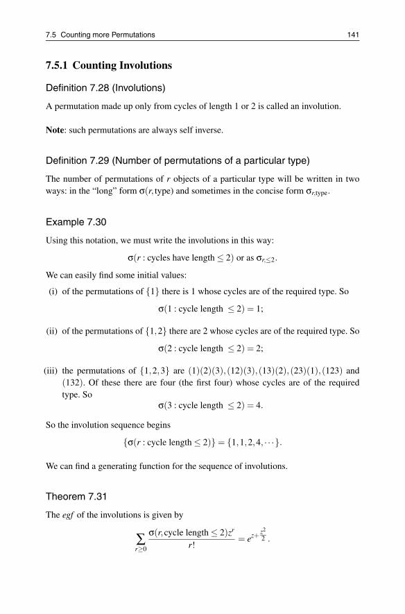
7.5 Counting more Permutations 141
7.5.1 Counting Involutions
Definition 7.28 (Involutions)
A permutation made up only from cycles of length 1 or 2 is called an involution.
Note: such permutations are always self inverse.
Definition 7.29 (Number of permutations of a particular type)
The number of permutations of r objects of a particular type will be written in twoways: in the “long” form σ(r, type) and sometimes in the concise form σr,type.
Example 7.30
Using this notation, we must write the involutions in this way:
σ(r : cycles have length ≤ 2) or as σr,≤2.
We can easily find some initial values:
(i) of the permutations of {1} there is 1 whose cycles are of the required type. So
σ(1 : cycle length ≤ 2) = 1;
(ii) of the permutations of {1,2} there are 2 whose cycles are of the required type. So
σ(2 : cycle length ≤ 2) = 2;
(iii) the permutations of {1,2,3} are (1)(2)(3),(12)(3),(13)(2),(23)(1),(123) and(132). Of these there are four (the first four) whose cycles are of the requiredtype. So
σ(3 : cycle length ≤ 2) = 4.
So the involution sequence begins
{σ(r : cycle length ≤ 2)} = {1,1,2,4, · · ·}.
We can find a generating function for the sequence of involutions.
Theorem 7.31
The egf of the involutions is given by
∑r≥0
σ(r,cycle length ≤ 2)zr
r!= ez+ z2
2 .

142 7. Exponential Generating Functions
Proof
An involution has either 0 fixed points and all its other cycles of length 2; or 1 fixedpoint and all its other cycles of length 2, and so on. This means we can constructinvolutions as in Figure 7.2.
Figure 7.2 Involutions.
If we look carefully at the formula in the figure it is seen to be in the form ofTheorem 7.12 – that is, as the product of two egf s:
(i) the first part of the product is the egf of the number of permutations which aremade up only from fixed points. There is always only one such permutation (theidentity) and so
∑r≥0
σ(r,cycle length is 1)zr
r!= ∑
r≥0
zr
r!= ez;
(ii) the second part of the product is the egf of the number of permutations all ofwhose cycles are of length 2. But we know how to count these (Theorem 4.18)
σ(r : cycle length is 2) =
{0 if r is odd;(2m)!2mm! when r = 2m.
This means that its egf is
∑r≥0
σ(r : cycle length is 2)zr
r!= ∑
s≥0
(2s)!2ss!
z2s
(2s)!= ∑
s≥0
(z2)s
2ss!= e
z2
2 .
Finally, putting this all together, we have
∑r≥0
σ(r,cycle length ≤ 2)zr
r!= ez · e
z2
2 = ez+ z2
2 .

7.5 Counting more Permutations 143
From this it is easy to derive a recurrence as in the following example.
Example 7.32
We simply differentiate the egf (using concise notation):
∑r≥0
σr,≤2zr
r!= ez+ z2
2
which gives
∑r≥0
σr+1,≤2zr
r!= (1+ z)ez+ z2
2 = (1+ z) ∑r≥0
σr,≤2zr
r!
and, if we compare coefficients of zr on either side, then
σr+1,≤2
r!=
σr,≤2
r!+
σr−1,≤2
(r−1)!
and hence the required result
σr+1,≤2 = σr,≤2 + rσr−1,≤2.
There is an enumerative argument for the same recurrence.
Example 7.33
The number of involutions of r−1 objects is σr−1,≤2. If we introduce a new elementr there will be σr,≤2 involutions. However, in introducing the new element there aretwo possibilities for it: either it makes its own cycle (so it becomes a fixed point),or it takes one of the existing fixed elements and together they make a 2 cycle as inFigure 7.3. Hence, overall
Figure 7.3 Constructing involutions.

144 7. Exponential Generating Functions
σr,≤2 = σr−1,≤2 +(r−1)σr−2,≤2.
Using this recurrence with the initial values σ0,≤2 = 1 and σ1,≤2 = 1 the sequencecontinues
{σr,≤2} = {1,1,2,4,10,26, · · ·}.
This leads to a very natural companion to this result – counting the number ofpermutations, each of whose cycles are of length 3 or more.
Example 7.34
The number of such permutations is σ(r : cycle length > 2) = σr,>2. In Figure 7.4 weconstruct the totality of permutations by bringing together the two different types ofpermutation (involutions with those whose cycles are of length 3 or more).
Figure 7.4 Constructing permutations.
We may
(i) choose k elements from r objects in(r
k
)ways and there are σk,≤2 permutations of
these elements, whose cycles are all of length 2 or less;
(ii) there are σr−k,>2 permutations of the remaining elements all of whose cycles areof length greater than 2.
Now we appeal to the product formula (Theorem 7.12) and then we have:
11− z
=
(∑r≥0
σr,≤2 zr
r!
)(∑r≥0
σr,>2 zr
r!
)
and a simple rearrangement gives
∑r≥0
σr,>2 zr
r!=
e−z− z2
2
1− z.
The number of permutations all of whose cycles are of length 3 or more satisfies arecurrence. You will be invited to derive this from the egf in Exercise 7.19. We givean enumerative derivation – with a vital dash of algebra.

7.5 Counting more Permutations 145
Example 7.35
We take as the elements to be permuted {1,2, . . . ,r}. There are σr,>2 such permuta-tions. The element 1 belongs to a cycle of length 3 or more – so it belongs to a cycleof length 3, or 4, or 5, and so on:
(i) suppose it belongs to a 3 cycle. There are (r − 1)(r − 2)σr−3,>2 such permuta-tions, since there are(r− 1)(r− 2) 3 cycles containing the element 1, while theremaining elements can be permuted in σr−3,>2 ways;
(ii) next, suppose the element 1 belongs to a 4 cycle. There are (r − 1)(r − 2)(r −3)σr−4,>2 such permutations.
If we continue this argument, then we have:
σr,>2 = (r−1)(r−2) [σr−3,>2 +(r−3)σr−4,>2 +(r−3)(r−4)σr−5,>2 + · · · ]= (r−1)(r−2)σr−3,>2 +(r−1)[(r−2)(r−3)σr−4,>2 + · · · ]= (r−1)(r−2)σr−3,>2 +(r−1)σr−1,>2
and so the required recurrence is
σr,>2 = (r−1)σr−1,>2 +(r−1)(r−2)σr−3,>2.
Using the recurrence with the initial values σ0,>2 = 1, σ1,>2 = 0, and σ2,>2 = 0 thesequence continues
{σr,>2} = {1,0,0,2,6,24, . . .}.
7.5.2 Counting Zig-Zag Permutations
We can also count permutations whose image – in the bijective form – has a particularform, just as we counted ascents in Chapter 5. This next example concerns permuta-tions whose image alternately rises and then falls. It has a very surprising egf.
Definition 7.36 (Zig-zag permutations)
The zig-zag permutations are those that begin with a rise and thereafter alternately fallfollowed by a rise and so on.
Example 7.37
The permutation (1)(23)(45) may be written in bijective form(
11
23324554
);

146 7. Exponential Generating Functions
this is a zig-zag permutation, since the image goes 1 ↗ 3 ↘ 2 ↗ 5 ↘ 4 as required.
Example 7.38
Now we construct a recurrence satisfied by the zig-zag numbers. In counting such per-mutations we observe that the odd and even cases are different, as Figure 7.5 shows.
Figure 7.5 Zig-zag permutations.
We deal with the odd case first. Suppose that there are or zig-zag permutations ofthe set {1,2,3, . . . ,r} and r is even. We may introduce an additional element r + 1which is then odd. We can construct the zig-zag permutations of the enlarged set{1,2,3, . . . ,r,r + 1}, and there are or+1 of them, by placing this (largest) elementamongst the elements of the original set. It may be placed at any position but thefirst and last – these would give a descent and an ascent respectively. Further, it mustbe placed at an even indexed position. Then we construct the zig-zag permutations asin Figure 7.6. So now we have
Figure 7.6 Odd zig-zag permutation.

7.5 Counting more Permutations 147
or+1 = ∑k odd
(rk
)okor−k.
However, if we agree that or = 0 whenever r is even (including zero), then we canwrite this (for r ≥ 1)
or+1 = ∑k>0
(rk
)okor−k, with o1 = 1.
If we consider the even case er and agree that er = 0, whenever r is odd, we findby a similar enumeration that
er+1 = ∑k>0
(rk
)oker−k.
The latter recurrence is “mixed”. However, both recurrences may be used to derivetheir respective egf s.
Theorem 7.39 (Egf of the zig-zag numbers)
The egf of the zig zag numbers {ar} is
Z(z) = O(z)+E(z) = ∑r≥0
arzr
r!= tanz+ secz.
Proof
We start with the first recurrence. Again we recognize the result of a product of egf sand making use of Theorem 7.12 gives
∑r≥0
or+1zr
r!=
(∑r≥0
orzr
r!
)(∑r≥0
orzr
r!
)+1
= (O(z))2 +1.
But the term on the left (from Theorem 7.9) may be rewritten as a derivative and thenwe have a differential equation with a unique solution
O′(z) = (O(z))2 +1
⇒ O(z) = tanz.
Working in the same way on the second recurrence gives E(z) = secz.

148 7. Exponential Generating Functions
7.5.3 Exercises
Exercise 7.11
Show that the sequence {σr,=2}, which counts the number of permutations ofr elements that consist only of cycles of length 2:
(i) satisfies the recurrence σr+1,=2 = rσr−1,2
(ii) deduce that σ2r,=2 = 1.1.3. · · · .(2r−1).
Exercise 7.12
Show that:
(i) the egf of the sequence {σ(r : all cycles of length 3)} which counts thenumber of permutations whose cycles are all of length 3 is
∑r≥0
σr,=3zr
r!= e
z3
3 ;
(ii)
σr,�3 = ∑k�0
(rk
)σk,=3σr−k,�2.
Deduce that the egf of the sequence {σ(r : cycles of length ≤ 3)} is
∑r≥0
σr,≤3zr
r!= ez+ z2
2 + z3
3 .
We could continue this process – of which sequence is the function
ez+ z2
2 + z3
3 + z4
4 +···
the egf ?
Exercise 7.13
By differentiating the egf of the sequence {σ(r : all cycles of length 2)} twice,show that the terms of this sequence also satisfy the recurrence σr+2,=2 =σr,=2 + r(r−1)σr−2,=2.
7.6 Miscellaneous Exercises
Exercise 7.14
Find the ratio (as r → ∞) of the number of push-button lock combinations {cr}to the number of permutations.

7.6 Miscellaneous Exercises 149
Exercise 7.15
Show that the egf of the sequence {σ(r : no cycles of length 2)} ≡ {σr, =2} is
∑r≥0
σr, =2zr
r!=
e−z2
2
1− z.
By differentiating this, show that the sequence satisfies the recurrence
σr+1, =2 = (r +1)σr, =2 − rσr−1, =2 + r(r−1)σr−2, =2.
Exercise 7.16
Establish the identity
cr = ∑k�0
(rk
)2r−kdk,
in which {cr} is the push-button lock sequence and {dr} is the derangementsequence.
Exercise 7.17
The two recurrences for the (odd/even) zig-zag numbers can be used to find theinitial numbers of these permutations. Given that
(i) o0 = 0 and o1 = 1, show that the odd zig-zag numbers continue {or} ={0,1,0,2,0,16,0,272, . . .};
(ii) e0 = 1 and e1 = 0, show that the even zig-zag numbers continue {er} ={1,0,1,0,5,0,61, . . .}.
Exercise 7.18
The sequence {ur} has (a sort of) egf
∑r≥0
ur+1zr
r!=
e−z
(1− z)2 .
Prove that it satisfies the two recurrences:
(i) ur+1 = rur +dr where {dr} is the derangement sequence;
(ii) ur+2 = (r +1)ur+1 + rur.
Find the first five terms of the sequence. (This sequence counts the number ofpermutations of {1,2, . . . ,r} that have no sub-strings of the form . . .k,k+1, . . .
for any k, in which 0 ≤ k ≤ r−1.)

150 7. Exponential Generating Functions
Exercise 7.19
Show (from the egf ) that the recurrence satisfied by the number of permutationsthat are not involutions σr,>2 is
σr,>2 = (r−1)σr−1,>2 +(r−1)(r−2)σr−3,>2.
Exercise 7.20
Use the recurrence of Example 7.38 for the even zig-zag numbers
er+1 =r
∑k=0
(rk
)oker−k
to derive its egf.

8Graphs
8.1 Introduction to Graphs
In this chapter we will introduce the idea of graphs, but these are not the pictures withaxes and lines which you may have been used to. This use of the word graph representsa collection of vertices and of edges. They are usually shown as very simple pictures,where the vertices are represented by dots and edges by lines.
We begin by drawing some simple graphs – see Figure 8.1. Then we will givea more formal definition of what we mean. In these examples one can see that thevertices are {a,b,c}. Each graph has the same set of vertices but different sets ofedges. So to define a graph we need to say what the vertices are and what the edgesare.
Definition 8.1 (Graph)
A graph Γ is defined as a pair (V, E) where E is a subset of unordered pairs of elementsfrom V . V is called the set of vertices and E is called the set of edges. If e = (u,v) isan edge then the vertices u and v are the endpoints of e.
A graph satisfying this definition is sometimes called a simple graph, as we allowno loops, that is edges which begin and end at the same vertex. We also do not allowmultiple edges: that is, between two vertices u and v there is at most one edge. Oneway to define a graph is just to list the edges. Table 8.1 gives the lists for the graphsshown in Figure 8.1:
A. Camina, B. Lewis, An Introduction to Enumeration,Springer Undergraduate Mathematics Series,DOI 10.1007/978-0-85729-600-9 8, © Springer-Verlag London Limited 2011
151
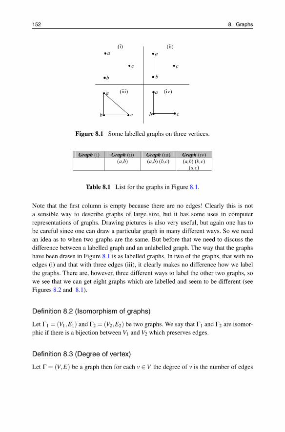
152 8. Graphs
Figure 8.1 Some labelled graphs on three vertices.
Table 8.1 List for the graphs in Figure 8.1.
Note that the first column is empty because there are no edges! Clearly this is nota sensible way to describe graphs of large size, but it has some uses in computerrepresentations of graphs. Drawing pictures is also very useful, but again one has tobe careful since one can draw a particular graph in many different ways. So we needan idea as to when two graphs are the same. But before that we need to discuss thedifference between a labelled graph and an unlabelled graph. The way that the graphshave been drawn in Figure 8.1 is as labelled graphs. In two of the graphs, that with noedges (i) and that with three edges (iii), it clearly makes no difference how we labelthe graphs. There are, however, three different ways to label the other two graphs, sowe see that we can get eight graphs which are labelled and seem to be different (seeFigures 8.2 and 8.1).
Definition 8.2 (Isomorphism of graphs)
Let Γ1 = (V1,E1) and Γ2 = (V2,E2) be two graphs. We say that Γ1 and Γ2 are isomor-phic if there is a bijection between V1 and V2 which preserves edges.
Definition 8.3 (Degree of vertex)
Let Γ = (V,E) be a graph then for each v ∈ V the degree of v is the number of edges
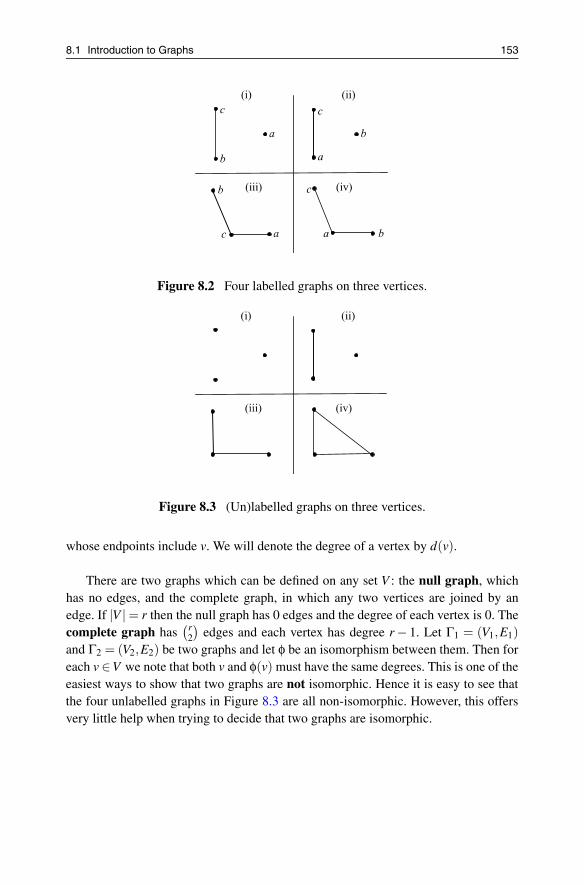
8.1 Introduction to Graphs 153
Figure 8.2 Four labelled graphs on three vertices.
Figure 8.3 (Un)labelled graphs on three vertices.
whose endpoints include v. We will denote the degree of a vertex by d(v).
There are two graphs which can be defined on any set V : the null graph, whichhas no edges, and the complete graph, in which any two vertices are joined by anedge. If |V |= r then the null graph has 0 edges and the degree of each vertex is 0. Thecomplete graph has
(r2
)edges and each vertex has degree r − 1. Let Γ1 = (V1,E1)
and Γ2 = (V2,E2) be two graphs and let φ be an isomorphism between them. Then foreach v ∈V we note that both v and φ(v) must have the same degrees. This is one of theeasiest ways to show that two graphs are not isomorphic. Hence it is easy to see thatthe four unlabelled graphs in Figure 8.3 are all non-isomorphic. However, this offersvery little help when trying to decide that two graphs are isomorphic.

154 8. Graphs
Lemma 8.4
Let Γ = (V,E) and |V | = r. Then there are two vertices with the same degree.
Proof
There are r vertices and the degrees have to come from the set {0,1, . . . ,r−1}. If thereis a vertex of degree 0 there is not one of degree r−1. So we are choosing r numbersfrom a set with only r − 1 elements. So we know two of the degrees have to be thesame by the pigeonhole principle (Theorem 1.12). If there are no vertices the degreescome from the set {1, . . . ,r−1} and the same proof works.
Example 8.5
An intriguing example concerns a group of people at a party. We draw the graph Γ sothat each person is a vertex and two people are joined if they know each other. Fromthe above lemma one can see that there are at least two people who know the samenumber of people.
Next we have a simple counting lemma.
Lemma 8.6
Let Γ = (V,E) be a graph and let |E| = m. Then
∑v∈V
d(v) = 2m.
Proof
Just note that each edge has exactly two vertices and each vertex v will be countedexactly d(v) times.
A simple consequence of this lemma is that there must be an even number ofvertices with odd degree otherwise the sum of the degrees has to be odd.
Example 8.7
Another example is to consider road systems in a country. We may construct a graphdefining the towns as the vertices and the roads as the edges connecting them. In thiscase we have to assume that there is at most one road connecting any two towns so asto make the graph simple. To decide whether one can travel from one town to another

8.1 Introduction to Graphs 155
we only need to know that there exists at least one route. We might also considerrailway lines, flight connections, rivers or canals rather than roads.
This example motivates the following definition.
Definition 8.8 (Paths in a graph)
Let Γ = (V,E) be a graph. A path in a graph is a sequence (v0,e1,v1, . . . ,en,vn)where each vi ∈ V and each ei ∈ E where the endpoints of ei are vi−1 and vi fori∈ {0,1, . . . ,n}. The length of such a path is n. Given such a path (v0,e1,v1, . . . ,en,vn)we define the following:
(i) the vertices v0 and vn are said to be connected;
(ii) a path is called a cycle if v0 = vn;
(iii) a simple path is a path in which ei �= e j ∀1 ≤ i, j ≤ n;
(iv) a simple closed path or simple closed cycle is a simple path which is a cycle.
If loops and multiple edges are allowed we have to be more careful with the definitionswe adopt.
Lemma 8.9
Let Γ = (V,E) be a graph. The relation “is connected” is an equivalence relation.
Proof
The reflexivity and symmetry are trivial. Let u and v be connected by the path(v0,e1,v1, . . . ,en,vn) so that u = v0 and v = vn and let v and w the connected by thepath (u0, f1,u1, . . . , fm,um) where v = u0 and w = um. Now it is easy to see that we canjust join the two paths and then u and w are connected.
Definition 8.10 (Connected component)
The equivalent classes are known as the connected components of the graph and ifthere is only one connected component the graph is said to be connected.
Clearly the null graph on n vertices has n connected components and the completegraph has just one.

156 8. Graphs
Definition 8.11 (Subgraph)
Let Γ = (V,E) be a graph. A subgraph of Γ is a subset of the vertices and edges so thatif an edge e is in the subgraph then so are both of its endpoints.
In using induction, it is often useful just to delete an edge or a vertex. If a vertex isdeleted, all the edges connected to the vertex also have to be deleted. We will use thenotation Γ\ x to denote such a subgraph, where x is a vertex or an edge.
Definition 8.12 (Bipartite)
A graph Γ = (V,E) is said to be bipartite if there exists a partition of V into two disjointsubsets, say U and W such that both U and W are null graphs. The union of the twosubgraphs U ∪W is called the bipartition.
Another way to say this is to say that for any edge e one endpoint is in U and the otheris in W .
Example 8.13
Given two natural numbers m and n, the complete bipartite graph, denoted by Km,n,is the graph with V = U ∪W and E = {(u,w) : u ∈ U, w ∈ W} where |U | = m and|V | = n.
Example 8.14
Let U be any set and let W be a collection of subsets of U . The graph Γ = (V,E) isdefined by V = U ∪W and E = {(u,w) : u ∈U, w ∈W with u ∈ w}.
Lemma 8.15
A graph Γ = (V,E) is bipartite if and only if it has no closed simple path of odd length.
Proof
Assume Γ = (V,E) is bipartite with V =V1∪V2 and let (v0,e1,v2, . . . ,en,vn) be a cycle.Assume without loss of generality that v0 ∈V1. Then v1 ∈V2, v2 ∈V1 and vi ∈Vi+1. Ifn is odd then vn ∈V2 and so cannot be equal to v0.
Now assume that Γ = (V,E) has no odd closed simple paths. We prove that if Γis connected it is bipartite and then it follows if the graph is disconnected by lookingat each connected component. For any pair of vertices, v and w say, define d(v,w) to

8.1 Introduction to Graphs 157
be the length of the shortest path from v to v, let d(v,v) = 0,∀v ∈V . Define a relationon V by v ∼ w if d(v,w) is even. We need to show that this is an equivalence relation.It is clearly reflexive and symmetric. So we need to consider transitivity. Let w1 ∼ w2
and w2 ∼ w3, that is both d(w1,w2) and d(w2,w3) are even. Assume that d(w1,w3) isodd. If we join the three paths there is a cycle of odd length, but it might have bothrepeated edges and repeated vertices. Assume that there is a repeated edge and choosethe first repeat, (vi−1,ei,vi, . . . ,en,vn), where ei = en. So vn−1 = vi−1 and vn = vi. If(vi−1,ei,vi, . . . ,en−1,vn−1) has odd length then this is an odd simple closed path, whichis not allowed. Hence the length is even and we can just delete the section and stillhave a cycle of odd length. So we can assume that there are no repeated edges.
We can now repeat the argument for repeated vertices. If the first repeat is(vi−1,ei,vi, . . . ,en,vn) with vi−1 = vn and the length is odd then there is an odd simpleclosed path. If not we can delete this part an get a shorter odd cycle.
So ∼ is an equivalence relation. Let the two equivalence classes be V1 and V2. Notethat if two vertices are in the same equivalence class there cannot be an edge betweenthem because that would give a path of length 1.
One last definition in this section.
Definition 8.16 (Complement)
Given a graph, Γ = (V,E), the complement to Γ is the graph with the same verticeswhere two vertices are joined in the complement if and only if they are not joined inΓ.
This is often a nice way to construct new graphs from old.
8.1.1 Exercises
Exercise 8.1
Show that if Γ is a graph such that every vertex has odd degree then Γ has aneven number of vertices.
Exercise 8.2
Let Γ = (V,E) be a graph and assume that the degree of each vertex is at least1. Show that if the number of edges is less than the number of vertices there isa vertex of degree 1.
Exercise 8.3
Let Γ = (V,E) be a connected graph with at least two vertices. Show that thedegree of each vertex is at least 1.

158 8. Graphs
Exercise 8.4
Prove that if there is a path from u to v then there is a simple path from u to v.
Exercise 8.5
Let Γ = (V,E) be a bipartite graph with bipartition V = U ∪W . Assume that|V | = n, |E| = m, |U | = r and |W | = s. Show that
(i) m ≤ rs,
(ii) m ≤ n2
4 and
(iii) describe the graphs for which equality holds.
8.2 Connectivity
We wish to examine the concept of a connected graph, Definition 8.10, more care-fully. Can we construct a way of determining how connected a graph is? We do thatby turning a connected graph into a disconnected graph – we measure how connecteda graph is by how many edges or vertices it is necessary to remove before the graphbecomes disconnected. This idea is clearly important in many areas. If you live some-where where there is only one road out of your village and it gets cut off, you aretrapped. When you log on to the web, you hope that if one of the nodes that you needto connect you is offline, there are others which can be used. So we have the followingdefinitions.
Definition 8.17 (Separating Set)
Let Γ = (V,E) be a graph then
(i) A subset of vertices or edges is called a separating set if the graph with that subsetremoved is disconnected.
(ii) A graph is called k-connected if no subset of vertices of size k−1 is a separatingset but a subset of size k is.
(iii) A graph is called k-edge connected if no subset of edges of size k− 1 is a sepa-rating set but a subset of size k is.
It turns out that there are some interesting special cases.
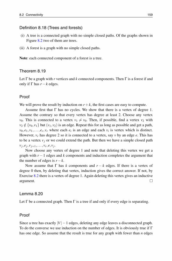
8.2 Connectivity 159
Definition 8.18 (Trees and forests)
(i) A tree is a connected graph with no simple closed paths. Of the graphs shown inFigure 8.2 two of them are trees.
(ii) A forest is a graph with no simple closed paths.
Note: each connected component of a forest is a tree.
Theorem 8.19
Let Γ be a graph with r vertices and k connected components. Then Γ is a forest if andonly if Γ has r− k edges.
Proof
We will prove the result by induction on r + k, the first cases are easy to compute.Assume first that Γ has no cycles. We show that there is a vertex of degree 1.
Assume the contrary so that every vertex has degree at least 2. Choose any vertexv0. This is connected to a vertex v1 �= v0. Then, if possible, find a vertex v2 withv2 /∈ {v0,v1} but (v1,v2) is an edge. Repeat this for as long as possible and get a path,v0,e1,v1, . . . ,er,vr where each ei is an edge and each vi is vertex which is distinct.However, vr has degree 2 so it is connected to a vertex, say v by an edge e. This hasto be a vertex v j or we could extend the path. But then we have a simple closed pathv j,e j,v j+1, . . . ,vr,e,v j.
Now choose any vertex of degree 1 and note that deleting this vertex we get agraph with r−1 edges and k components and induction completes the argument thatthe number of edges is r− k.
Now assume that Γ has k components and r − k edges. If there is a vertex ofdegree 0 then, by deleting that vertex, induction gives the correct answer. If not, byExercise 8.2 there is a vertex of degree 1. Again deleting this vertex gives an inductiveargument.
Lemma 8.20
Let Γ be a connected graph. Then Γ is a tree if and only if every edge is separating.
Proof
Since a tree has exactly |V |−1 edges, deleting any edge leaves a disconnected graph.To do the converse we use induction on the number of edges. It is obviously true if Γhas one edge. So assume that the result is true for any graph with fewer than n edges

160 8. Graphs
and assume Γ has r edges. Deleting an edge e leaves two disconnected components,but both will satisfy the hypothesis of the lemma. So both components are trees andthen adding e will give a tree.
Definition 8.21 (Independent paths)
A set of paths in a graph are called independent when they have no vertices in com-mon, except possibly the first and last vertices.
Theorem 8.22 (Menger’s Theorem)
Let Γ = (V,E) be a graph and let v and w be two connected vertices of V . Let k be thesize of the smallest set U of vertices with the property that v and w are not connectedin Γ\U . Let l be the largest number of independent paths from v to w. Then k = l.
Proof
Since removing the set U leaves v and w disconnected it is clear that l ≤ k. We willuse induction on k + |V | to show k ≤ l. So we have to show that there are at least kindependent simple paths from v to w. If k = 1 it is clear since there is a simple pathfrom v to w. So assume the result is true for all r < k.
Let U be a set of vertices with the property that v and w are not connected in Γ\Uand let |U | = k.
Assume that there is a vertex u ∈ U so that both vu and uw are edges. Now useinduction on the graph Γ\{u}. This says that there are k−1 independent simple pathsfrom v to w in Γ\{u} and we can add the path v,(vu),u,(uw),w to get k independentsimple paths.
Now assume that neither v nor w is joined to every vertex in U . For x ∈ {v,w} letΓx be the connected component of Γ\U containing x. Now construct a new graph Δv
which is constructed by taking Γv and joining U and all appropriate edges and one newvertex w′ joining w′ to all vertices in U . Note by the assumption w is not connected toevery vertex in U and so the graph Δv has fewer vertices than Γ. Also U disconnectsv and w′ so there are k independent simple paths from v to w′ and each one has to gothrough a different vertex in U . Now repeat the whole process, swapping the roles ofv and w and construct k independent simple paths from v′ to w each one going througha different vertex of U . Now take the path from v to a vertex in U from Δv and join itwith the path from that vertex to w in Δw to get k independent simple paths.
We are now left with the case when either v or w is joined to every vertex in U andwe can assume that this is true for any set of size k disconnecting v and w. So assumethat v is joined to each vertex in U . Choose one such vertex, say u, and consider thegraph Γ′ we get by deleting the edge vu. By induction there will be k − 1 disjoint

8.2 Connectivity 161
simple paths from v to w in Γ′, say {p1, p2, . . . , pk−1}. There is a simple path in Γfrom u to v and if this were independent of the k − 1 paths in Γ′ we would have kindependent paths. So any path from u to w has to have a vertex in common with someexisting independent path. For each path, say {q1,q2, . . . ,qr}, from u to w assumethat it has points {vi : 1 ≤ i ≤ m} in common with pi. Now for any p j,k−1 ≥ j > 1choose a vertex on pi from the set {vi : 1 ≤ i ≤ m} not equal to either v or w. It is clearthat this set of vertices disconnects v and w but has only k− 1 elements, which is acontradiction.
Based on this we can prove a theorem known as Hall’s Marriage Theorem for areason that will become apparent in an exercise. However, in the original formulationwe have the following: X is a set and A is a family of subsets of X . Is it possible tofind a subset Y of X of size |A | such that for each A ∈ A there is a y ∈ A∩Y . Anotherway to describe this is to talk about matchings. A matching in a graph Γ is a set ofdisjoint edges. This is the same as independent edges in the sense that any edge can bethought of as a simple path. In particular, in a bipartite graph any matching is a set ofindependent simple paths connecting the two parts of the graph. If the bipartite graphhas parts of size m and n then the maximal size of a matching is min(m,n). The nextresult gives a condition for there to be a maximal matching.
It is clear that if we have such a set then for any subset S of A , |SA∈A A| ≥ |C |.The surprising thing is that this is also a sufficient condition. We can turn this intoa graph theory problem. We construct a bipartite graph as follows. Set V1 = A andV2 = X and the only edges are given by pairs (A,x), where x ∈ A and x ∈ X and A ∈ A .For any subset of vertices of a graph, say W , we denote by N(W ) the set of verticesadjoined to W . Now we have the following theorem from which the result that thecondition is sufficient follows.
Theorem 8.23 (Hall’s Marriage Theorem)
Let Γ(V,E) be a bipartite graph with partition V1 ∪V2 = V . Then there is a set ofdisjoint edges of size |V1| if and only if |N(U)| ≥ |U | for all subsets U of V1.
Proof
The necessity is clear from the argument above. Now join two new vertices to Γ, sayv1 and v2, so that vi is joined to all the vertices in Vi and no others, for 1 ≤ i ≤ 2.The condition that there are a set of disjoint edges is the same as saying that thereare independent paths from v1 to v2. By Theorem 8.22 there are not enough disjointedges for a matching of size |V1| if there is a separating set of size less than |V1|. Sothere exists U1 ⊂V1 and U2 ⊂V2 with |U1|+ |U2| < |V1| and V1 \U1 is only joined to

162 8. Graphs
vertices in U2. We are almost there:
|N(V1 \U1| ≤ |U2| < |V1 \U1|.
This violates the condition that |N(U)| ≥ |U | for all U . So there are |V1| independentpaths form v1 to v2 which completes the proof.
Example 8.24
Another version of this problem is the assignment problem. That is given a number ofvacancies in a company and a number of people applying for the jobs, is it possibleto assign people to jobs so that every job is filled by someone who has applied for thejob? It depends on how many people apply for how many jobs as in Hall’s MarriageTheorem.
8.2.1 Exercises
Exercise 8.6
Let Γ be a connected graph. Show that if one edge is deleted then Γ has at mosttwo connected components.
Exercise 8.7
Let Γ be a graph with r vertices. Show that if each vertex has degree greaterthan r−1
2 then Γ is connected.
Exercise 8.8
Let Γ be a graph with r vertices. Show that if the sum of the degrees of twoadjacent vertices is greater than r−1 then Γ is connected.
Exercise 8.9
Given a graph Γ(V,E) we can construct the line graph LΓ which has as verticesE and two edges are joined if and only if they have a vertex in common. Usethe line graph to prove the edge version of Theorem 8.22.
Exercise 8.10
Prove that any tree is a bipartite graph.

8.3 Counting Graphs and Trees 163
8.3 Counting Graphs and Trees
We will divide this section into two subsections each devoted to graphs distinguishedby labels.
8.3.1 Counting Labelled Graphs and Trees
In this section we discuss some problems concerned with enumerating labelled graphs.We will find there is a considerable difference between labelled graphs and unlabelledgraphs. We begin with some easy results.
Proposition 8.25
(i) There are 2(r2) labelled graphs with r vertices;
(ii) There are((r
2)m
)labelled graphs with r vertices and m edges.
Proof
(i) We can choose any subset of the pairs of distinct vertices and join them.
(ii) This time we choose any subset of size m from the pairs of distinct vertices.
Let γr denote the number of labelled graphs with r vertices. Let γr,m denote the num-ber of labelled graphs with r vertices and m edges. The generating function (see Sec-tion 2.1) for γr,m, fixed r, is
(r2
)∑
m=0
γr,mzm = (1+ z)(r
2
).
Let cr denote the number of connected labelled graphs with r edges. Let
G(z) =∞
∑r=0
γnzr
r!, C(z) =
∞
∑r=1
crzr
r!
be the exponential generating functions (see Chapter 7) for cn and γn respectively.We want to show how γn and cn are related. To do this we introduce the idea of a
rooted graph. A graph is rooted if there is a chosen vertex which which will be calledthe root.

164 8. Graphs
Lemma 8.26
The number, cr, of labelled connected graphs with r vertices is given by
cr = 2(r
2
)− 1
r
r−1
∑k=1
k
(rk
)2(r−k
2 )ck. (8.1)
Proof
We count rooted graphs, noting that any labelled graph can be rooted at any of itsvertices, so the number of rooted connected graphs with r vertices is rγr. Each rootvertex lies in some component with say, k, vertices where 1 ≤ k ≤ r. The k vertices canbe labelled in any of
(rk
)ways. There are ck possible graphs for this component and
each can have any of its k vertices chosen as the root. The remaining r−k vertices cancome from γr−k possible graphs. Multiplying everything together and then summingover k gives
rγr =r
∑k=1
k
(rk
)γr−kck. (8.2)
But from Proposition 8.25 we know the numbers γk = 2(k
2
). Substituting this into the
equation above gives
r2(r
2
)=
r−1
∑k=1
k
(rk
)2(r−k
2
)ck + rcr.
Rearranging this equation gives the lemma.
This leads immediately to a surprisingly elegant relationship between the two ex-ponential generating functions.
Theorem 8.27
G(z) = exp(C(z)).
Proof
Differentiate exp(C(z)) to give C′(z)exp(C(z)). Now compare the coefficients of zr−1
in C′(z)G(z) and G′(z). Then using Equation (8.2) we see that the coefficients are thesame. So we have the equality C′(z)G(z) = G′(z). Solving this differential equationgives the result, as long as we define G(0) = 1 and C(0) = 0.

8.3 Counting Graphs and Trees 165
In this section we are going to count the number of labelled trees, a result that goesback to Cayley. There are many proofs of this result, but we will choose one that usesrecurrence. However, in this problem it is better to count forests, as this helps with therecurrence relation.
We will now count the number of labelled forests with r vertices and k componentswith a specified subset of size k which are in different components. We will let thisnumber be tr,k. By being labelled we mean that each vertex has a label.
Theorem 8.28
tr,k = krr−k−1
Proof
Let A be the specified subset and let v ∈ A have degree i. Deleting v and adding the ivertices connected to it to create a new set A′ gives a set of size k− i + 1. There aretr−1,k−1+i possible labelled forests that can be constructed with these parameters.
Do this for each possible set of size i from r − k vertices not in A and get thefollowing recurrence relation:
tr,k =r−k
∑0
(r− k
i
)tr−1,k−1+i.
The inductive hypothesis is
tr,k =r−k
∑0
(r− k
i
)(k−1+ i)(r−1)r−1−k−i.
Putting j = r− k− i
=r−k
∑0
(r− k
j
)(r−1− j)(r−1) j−1
=r−k
∑0
(r− k
j
)(r−1) j +
r−k
∑1
(r− k
j
)j(r−1) j−1
= rr−k +(r− k)r−k
∑1
(r− k−1
j−1
)(r−1) j−1
= rr−k +(r− k)r−k
∑0
(r− k−1
j
)(r−1) j
= rr−k +(r− k)rr−1−k = krr−1−k.

166 8. Graphs
Note that to make this work, the following definitions have to be made: t0,0 = tr,r = 0,and these cause no problems.
Corollary 8.29 (Cayley’s Theorem)
The number of labelled trees on r vertices is rr−2.
Proof
Note that tr,1 is just the number of labelled trees.
In the final part of this section we give another proof of Cayley’s theorem, thistime using the principle of inclusion–exclusion (see Section 1.3). We want to provethe following identity:
r−1
∑0
(−1)i(
bi
)(r− i)m = 0 (8.3)
when m < r. We are, however, going to prove something slightly stronger.
Proposition 8.30
The number of onto mappings from a set X with m elements to a set Y with r elementsis
r−1
∑0
(−1)i(
bi
)(r− i)m = 0
Proof
Let F be the set of all functions { f : X →Y}. For each element U ⊂Y let SU be the setof functions f ∈ F such that U is not in the image of f . Let S0 be the set of functionsf in which every y ∈ Y is in the image of f . Of course S0 is just the set we wish tocount, that is S0 = S /0. Then by Theorem 1.20 we get
#(S0) = #(S)− ∑#(U)=1
#(SU )+ ∑#(U)=2
#(SU )−·· ·+(−1)r#(SY ).
But #(SU ) = (r− k)m where #(U) = k since we are just mapping the set X into Y \U .Further there are
(rk
)choice for U of size k. So the above equation becomes
#(S0) = rm −(
r1
)(r−1)m +
(r2
)(r−2)m −·· ·
(rr
)(r− r)m.

8.3 Counting Graphs and Trees 167
Note that when m < r there is no onto mapping from X to Y so we get Equa-tion (8.3).
We now use this to get another proof of Cayley’s Theorem.
Theorem 8.31 (Cayley’s Theorem)
The number of labelled trees on r vertices is rr−2.
Proof
We now use inclusion–exclusion and induction. Let Tr be the set of trees on r vertices,which we will label 1,2, . . . ,r. We know that every tree has at least one vertex ofdegree 1 (see proof of Theorem 8.19). If r > 2 not all vertices can be of degree 1. Foreach 1 ≤ i1 < i2 · · · < ik ≤ r for 1 ≤ k ≤ r let Ti1,i2,...,ik be the set of trees so that eachof i1, i2, . . . , ik is a vertex of degree 1. Then by Theorem 1.20 we get
#(Tr) = ∑i
#(Ti)−∑i
#(Ti1<i2)+ · · ·+(−1)r ∑i1<i2···<ik
#(Ti1,i2,...,ir−1).
Now we can choose the k vertices i1 < i2 · · · ık in(r
k
)ways, but for each choice we
can connect to the remaining r− k vertices in (r− k)k different ways and those samer−k vertices can be made into a tree in #(Tr−k) ways. So the equation above becomes
#(Tr) =(
r1
)(r−1)#(T1)−
(r2
)(r−2)#(T2)+ · · ·+(−1)r
(r
r−1
)#(Tr−1)
=r−1
∑1
(−1)k−1(
rk
)(r− k)k#(Tr−k)
We now use induction and get
#(Tr) =r−1
∑1
(−1)k−1(
rk
)(r− k)k(r− k)r−k−2
=r−1
∑1
(−1)k−1(
rk
)(r− k)r−2.
This is just Equation (8.3) with m = r−2.
8.3.2 Counting Unlabelled Graphs
Example 8.32
A much harder question is how to count labelled graphs. One way to do this is tothink of a graph as a colouring of the pairs (u,v) with u �= v with Sn acting (see Theo-

168 8. Graphs
rem 6.27). So we need to evaluate the cycle index for Sym(n) acting on distinct pairs.For any given n this is possible but the general example is messy.
Let us consider the case of Sym(4). Table 8.2 represents the action.
Table 8.2 The symmetric group of degree 4 acting on pairs.
So the cycle index is:
P(X1,X2,X3,X4) =124
(X61 +6X2
1 X22 +8X2
3 +3X21 X2
2 +6X2X4).
If we replace each Xi with 2 we count the number of graphs on four vertices. Sowe have 11 graphs on four vertices. If, however, we want to see how many differentgraphs there are with a given number of edges we have to be more careful. So colourthe edges white if they are to be part of the graph and black if we want to excludedthem. We can then count using the cycle index to get the following expression (seeTheorem 6.27):
124
((B+W )6 +9(B+W )2(B2 +W 2)2 +8(B3 +W 3)2
)
+124
(6(B2 +W 2)(B4 +W 4)
). (8.4)
If we look for the coefficient of B3W 3 we find that it is 3, so there are three unlabelledgraphs on four vertices with three edges.
If we consider this example further we can see how to obtain the generating func-tion for the number of graphs on four vertices and i edges. Substitute 1 for B and z forW in Equation (8.4) (page 168), and get:
1+ z+2z2 +3z3 +2z4 + z5 + z6.
Theorem 8.33
Let Γ(V,E) be a graph and let G be the group of automorphisms on the vertices of Γ.Then we can label Γ in
|V |!|A|

8.3 Counting Graphs and Trees 169
ways.
Proof
Note that no non-trivial element of G will fix a labelled graph, since any change of thelabelling will give a new labelling. Also any graph can be labelled in |V |! ways. So byTheorem 6.4 it follows that the number of orbits of G on the set of labelled graphs is|V |!|A| .
We now look at an analogue to Theorem 8.27 for (un)labelled graphs. Let κn bethe number of connected graphs with n vertices and let gn be the number of graphswith n vertices. Let
K(x) =∞
∑n=0
κnzn and G(x) =∞
∑n=0
gnzn
be the ordinary generating functions. We wish to relate these but first we prove alemma.
Lemma 8.34
The number of graphs with kr vertices in which each connected component has rvertices is given by
∑(
κr
k0,k1,k2, . . . ,kκr
), (8.5)
where the sum is over all k0 + k1 + k2 + · · ·+ kκr = κr and k1 +2k2 + · · ·+ rkκr = k.
Proof
We know that there are κn possible connected graphs with r vertices and we need tochoose k of them. Recall that we can use repeats, but that the numbers of ways we canchoose will depend on how many are the same. So if we choose all the same there arejust κr choices, but if we have k−1 the same we can choose one of them in κr waysand the second in κr −1 ways.
We describe the choices this way: k0 are not chosen, k1 are chosen once, and ingeneral ki are chosen i times 0 ≤ i ≤ κn, where
∑i=0
ki = κr and ∑i=1
iki = k.
But if we think there are κr! choices we get k0!k1! · · ·kκr ! repeats. So the numberof choices is the multinomial coefficient
( κrk0,k1,···kκr
). This is similar to the result in
Theorem 5.1.

170 8. Graphs
The multinomial gets its name because it is the coefficient of a power of z when thereare more than two terms. The same argument as above shows that in the expansion of(z1 + z2 + · · ·+ zk)r the coefficient of the term zt1
1 zt22 · · ·ztk
k is ∑( r
t1,t2,...,tr
)where the sum
is over all k-tuples with t1 + t2 + · · ·+ tk = r.
Theorem 8.35
Let G(z) be the generating function for graphs and K(z) be the generating function forconnected graphs. Then
G(z) = exp
(∞
∑1
K(zk)k
)
Proof
By the preceding lemma and the remark above the generating function for graphs sothat each connected component has r vertices is given by
(1+ xr + x2r + x3r + · · ·)κr .
Note that a graph with all connected components with r vertices has kr vertices forsome k. Now consider the coefficient of xkr in the above expansion. It will be preciselythe sum:
∑(
κr
k0,k1,k2, . . . ,kκr
),
where the sum is over all k1 + k2 + · · ·+ kr = κr and k1 +2k2 + · · ·+ rkκr = k.Now
(1+ zr + z2r + z3r + · · ·)κr = (1− zr)−κr .
Now any graph will be the union of its connected components. We collect togetherthose of the same size and then multiply the generating functions for each set. So
G(z) =∞
∏r=1
((1− zr)−κr)
= exp
(∞
∑r=1
−κr log(1− zr)
)
= exp
(∞
∑r=1
∞
∑k=1
κrzrk
k
).
Now change the order of summation. This is valid since in the expression inside theexp the coefficient of any power of z is a finite sum:
= exp
(∞
∑k=1
(∞
∑r=1
κrzrk
k)
).
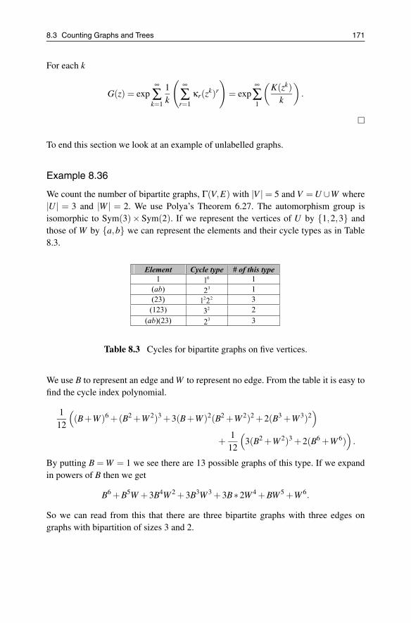
8.3 Counting Graphs and Trees 171
For each k
G(z) = exp∞
∑k=1
1k
(∞
∑r=1
κr(zk)r
)= exp
∞
∑1
(K(zk)
k
).
To end this section we look at an example of unlabelled graphs.
Example 8.36
We count the number of bipartite graphs, Γ(V,E) with |V | = 5 and V = U ∪W where|U | = 3 and |W | = 2. We use Polya’s Theorem 6.27. The automorphism group isisomorphic to Sym(3)× Sym(2). If we represent the vertices of U by {1,2,3} andthose of W by {a,b} we can represent the elements and their cycle types as in Table8.3.
Table 8.3 Cycles for bipartite graphs on five vertices.
We use B to represent an edge and W to represent no edge. From the table it is easy tofind the cycle index polynomial.
112
((B+W )6 +(B2 +W 2)3 +3(B+W )2(B2 +W 2)2 +2(B3 +W 3)2
)
+112
(3(B2 +W 2)3 +2(B6 +W 6)
).
By putting B = W = 1 we see there are 13 possible graphs of this type. If we expandin powers of B then we get
B6 +B5W +3B4W 2 +3B3W 3 +3B∗2W 4 +BW 5 +W 6.
So we can read from this that there are three bipartite graphs with three edges ongraphs with bipartition of sizes 3 and 2.

172 8. Graphs
8.3.3 Exercises
Exercise 8.11
Show that if a tree T with r vertices has exactly two vertices of degree 1 everyother vertex has degree 2. Show that such trees are isomorphic but that such atree can be labelled in r!/2 different ways.
Exercise 8.12
Let Γ be a connected graph. Prove that if each vertex of Γ has degree 2 then Γis a cycle. Find the exponential generating function for the number of labelledgraphs all of whose vertices have degree 2.
Exercise 8.13
Whilst there are three labelled trees on three vertices, how many unlabelledtrees are there on three vertices? What happens for four vertices?
Exercise 8.14
Let Γ be a graph whose vertex set is {1,2,3,4}. How many labelled forestswith two connected components are there?
Exercise 8.15
How many distinct graphs are there with five vertices?
8.4 Planarity
A very interesting class of graphs is those that can be drawn in the plane. Not allgraphs can be drawn in the plane: for example the complete graph on five verticescannot. There are number of ways to prove this, although playing around with penciland paper will soon convince you. But we should be more precise about what wemean.
Definition 8.37
A graph is called a plane graph if it can be drawn in the plane so that the edges aresimple curves which intersect only at its endpoints. A graph is called planar if it isisomorphic to a plane graph.
Obviously there is a topological aspect to this idea and we can think of a planargraph as one that can be embedded into the plane. Given a plane graph it divides the
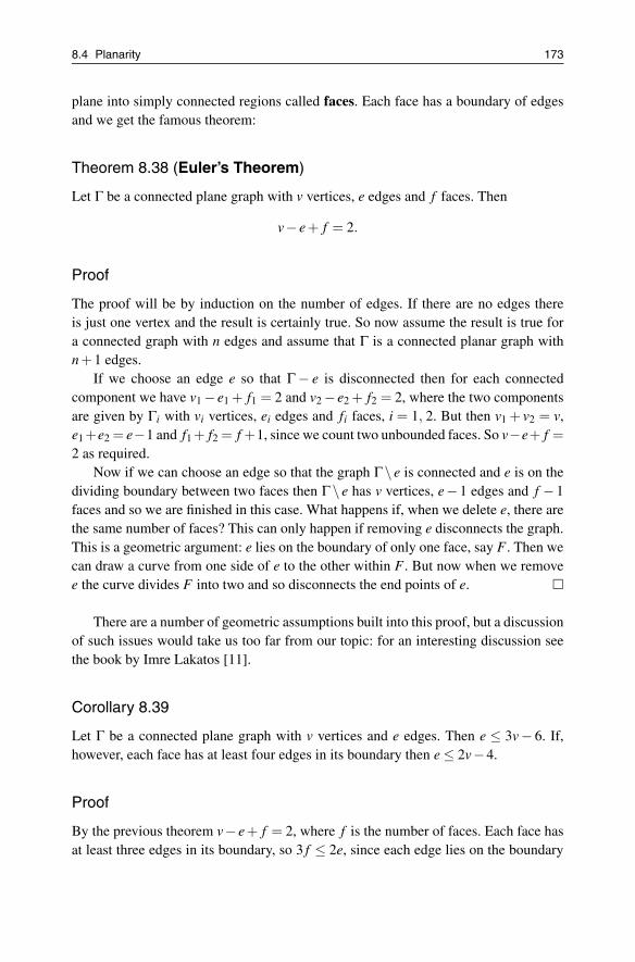
8.4 Planarity 173
plane into simply connected regions called faces. Each face has a boundary of edgesand we get the famous theorem:
Theorem 8.38 (Euler’s Theorem)
Let Γ be a connected plane graph with v vertices, e edges and f faces. Then
v− e+ f = 2.
Proof
The proof will be by induction on the number of edges. If there are no edges thereis just one vertex and the result is certainly true. So now assume the result is true fora connected graph with n edges and assume that Γ is a connected planar graph withn+1 edges.
If we choose an edge e so that Γ − e is disconnected then for each connectedcomponent we have v1 −e1 + f1 = 2 and v2 −e2 + f2 = 2, where the two componentsare given by Γi with vi vertices, ei edges and fi faces, i = 1, 2. But then v1 + v2 = v,e1 +e2 = e−1 and f1 + f2 = f +1, since we count two unbounded faces. So v−e+ f =2 as required.
Now if we can choose an edge so that the graph Γ\ e is connected and e is on thedividing boundary between two faces then Γ\ e has v vertices, e−1 edges and f −1faces and so we are finished in this case. What happens if, when we delete e, there arethe same number of faces? This can only happen if removing e disconnects the graph.This is a geometric argument: e lies on the boundary of only one face, say F . Then wecan draw a curve from one side of e to the other within F . But now when we removee the curve divides F into two and so disconnects the end points of e.
There are a number of geometric assumptions built into this proof, but a discussionof such issues would take us too far from our topic: for an interesting discussion seethe book by Imre Lakatos [11].
Corollary 8.39
Let Γ be a connected plane graph with v vertices and e edges. Then e ≤ 3v− 6. If,however, each face has at least four edges in its boundary then e ≤ 2v−4.
Proof
By the previous theorem v− e+ f = 2, where f is the number of faces. Each face hasat least three edges in its boundary, so 3 f ≤ 2e, since each edge lies on the boundary

174 8. Graphs
of at most two faces. Now substitute in the above 3 f = 6−3v+3e ≤ 2e, which givesthe corollary.
The second part follows similarly.
Example 8.40
The complete graph on five vertices has 10 edges. But 10 > 15− 6, so the completegraph on five vertices is not planar.
Example 8.41
The complete bipartite graph on six vertices has nine edges. But 9 < 18− 6, so thiscriterion is not sufficient to exclude this graph from being planar. However, 9 > 12−4,so the second condition shows that the complete bipartite graph is not planar.
8.4.1 Exercises
Exercise 8.16
The girth g of a graph is defined to be the length of the shortest cycle in a graph.Let Γ be a graph with v vertices and e edges. Show that if Γ is planar then
(g−2)e ≤ g(v−2).
Exercise 8.17
Show that every planar graph has a vertex of degree at most 5.
Exercise 8.18
Let Γ be a plane graph with less that 12 faces and every vertex has degree atleast 3. Show that there is a face with no more than four edges in the boundary.
Exercise 8.19
Prove that if a graph Γ has more than 11 vertices then both Γ and its comple-ment cannot be planar.
Exercise 8.20
A simple graph is called maximal planar if it is planar but adding any edge (onthe given vertex set) would destroy that property. Show that all faces (even theouter one) are then bounded by three edges. Show that in this case that if thegraph has v vertices with v > 2, then it has precisely 3v− 6 edges and 2v− 4faces.

8.5 Miscellaneous Exercises 175
8.5 Miscellaneous Exercises
Exercise 8.21
Let Γ = (V,E) be a graph on six vertices. Show that either Γ or its complementhas a triangle as a subgraph.
Exercise 8.22
Let Γ = (V,E) be a connected graph. The diameter d of a graph is the maximumdistance apart of two vertices. If the maximal degree of any vertex is m provethat the number of vertices is bounded by
1+m(m−1)d −1
m−2.
Exercise 8.23
Given a set of n men and a set of n women, let each man make a list of thewomen he is willing to marry. Then each man can be married to a woman onhis list if, and only if, for every value of k(1 ≤ k ≤ n) the union of any k of thelists contain at least k names.
Exercise 8.24
A group of friends buy a pizza and argue about how many pieces it can be cutinto with a given number of cuts. Given that the pizza is circular and they usen cuts, find a formula for the maximum number of pieces.
Exercise 8.25
How many bipartite graphs with bipartitions of size 2 and 4 are there (seeExample 8.36)?

9Partitions and Paths
9.1 Introducing Partitions
The shopkeeper’s problem – giving change to a customer who offers an amount ofmoney for a particular purchase – leads to a very sophisticated mathematical idea.Given one positive integer (the difference between the amount offered and the costof the item) how many ways are there to write this (give change) as a sum of otherpositive integers?
Definition 9.1 (Partition)
A partition of a positive integer r by a set of positive integers A is a sum in which,
r = ∑ai∈A
λiai
and each λi is a positive integer.
Giving change has no natural order, so the partitions of interest in this chapter are theunordered partitions (see Exercise 2.7, which deals with ordered partitions). When-ever the word partition is used in this chapter, we mean an unordered partition. Asalways, our interest will be to enumerative: in this case, to count the number of un-ordered partitions of an arbitrary positive integer, making use of a specified coinage.
A. Camina, B. Lewis, An Introduction to Enumeration,Springer Undergraduate Mathematics Series,DOI 10.1007/978-0-85729-600-9 9, © Springer-Verlag London Limited 2011
177

178 9. Partitions and Paths
Example 9.2
We find the number of ways there are to partition (without regard to order) a givenpositive integer r using the positive integers 1 and 2. A generating function does theenumeration for us: we seek the coefficient of zr in the product shown in Figure 9.1.
Figure 9.1 Partitions using {1,2}.
If we begin to multiply out this product, we can find the number of such partitionsfor initial values of r:
1+ z+2z2 +2z3 +3z4 +3z5 +4z6 +4z7 + · · · .
A little thought should convince you that in order to be sure of the coefficient of zr wemust at least go as far as this power in each bracket.
In fact we can sidestep such a tedious expansion altogether.
Example 9.3
The expressions above may be written (1+z+z2 +z3 +· · ·) and (1+z2 +z4 +z6 +· · ·).We can rewrite this as
(1+ z+ z2 + z3 + · · ·)(1+ z2 + z4 + z6 + · · ·) =1
(1− z)(1− z2).
Next we decompose this using partial fractions; it becomes
(1+ z+ z2 + z3 + · · ·)(1+ z2 + z4 + z6 + · · ·) = 14
(2
(1− z)2 +1
1− z+
11+ z
).
It is now an easy matter to pick out the required coefficient of zr as
14 (2(r +1)+1+(−1)r) =
2r +3+(−1)r
4
and this is the required (explicit) answer. In fact we may write the answer in a morecompact form, using the floor function
Number of such partitions =⌊
r2
⌋+1.

9.1 Introducing Partitions 179
We can use the same basic ideas on a slightly more sophisticated example.
Example 9.4
A country has just three coins: a 1 cent coin, a 2 cent coin and a 4 cent coin – this isa very mathematical country. We seek the number of ways that change may be givenfor 100 cents. We do this by finding the coefficient of z100 in the generating function
(1+ z+ z1+1 + z1+1+1 · · ·)(1+ z2 + z2+2 + z2+2+2 · · ·)(1+ z4 + z4+4 + z4+4+4 · · ·)= (1+ z+ z2 + · · ·)(1+ z2 + z4 + · · ·)(1+ z4 + z8 + · · ·)
Each of the bracketed expressions is an infinite GP and so for |z| < 1 we may rewriteit
=1
(1− z)(1− z2)(1− z4).
Now we use partial fractions and find that
=1
8(1− z)3 +1
4(1− z)2 +9
32(1− z)+
1
16(1+ z)2 +5
32(1+ z)+
1+ z8(1+ z2)
.
We may expand each term on the right using the Binomial Theorem; the coefficient ofz100 is
18
(102
2
)+ 1
4
(101
1
)+ 9
32 + (−1)100
16
(101
1
)+ 5(−1)100
32 + (−1)50
8 = 676.
Time to introduce some notation.
Definition 9.5 (Notation for partitions)
Given a set A of positive integers, the number of partitions of the positive integer r is
(i) written p(r : A);
(ii) the “summands” in a partition are called parts.
Now we extend the results of Example 9.4 by seeking the number of ways to givechange for an arbitrary amount, using the same coinage.

180 9. Partitions and Paths
Example 9.6
The number of ways we can give change for an arbitrary amount (r cents) is simplyp(r : {1,2,4}). But we already know the generating function for this:
∑r�0
p(r : {1,2,4})zr =1
(1− z)(1− z2)(1− z4).
Again, we use partial fractions and as before
∑r�0
p(r : {1,2,4})zr =1
8(1− z)3 +1
4(1− z)2 +9
32(1− z)
+1
16(1+ z)2 +5
32(1+ z)+
1+ z8(1+ z2)
.
We may expand each term on the right; the coefficient of zr is complicated by the lastthree terms. We start with the final term since this determines how we deal with theother two:
1+ z8(1+ z2)
=18(1+ z)(1+ z2)
−1= 1
8
(1+ z− z2 − z3 + z4+ · · ·
)
so the coefficient of zr from this term is{ 18 if r = 0,1(mod 4);
− 18 if r = 2,3(mod 4).
This tells us that we need to consider the remaining terms also in terms of residueclasses mod 4:
1
16(1+ z)2 =116 ∑
r≥0
(−1)r(
r +11
)zr
so the coefficient of zr from this term is{ r+116 if r = 0,2(mod 4);
− r+116 if r = 1,3(mod 4).
Finally5
32(1+ z)=
532 ∑
r≥0
(−1)rzr
so the coefficient of zr from this term is{ 532 if r = 0,2(mod 4);
− 532 if r = 1,3(mod 4).
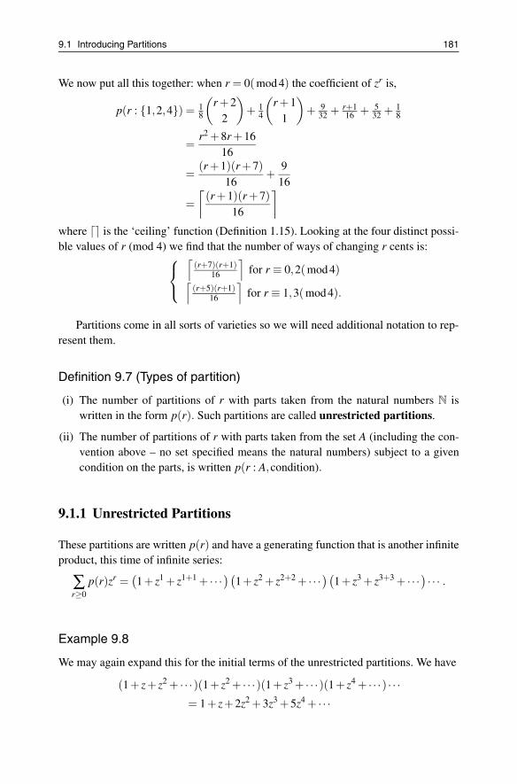
9.1 Introducing Partitions 181
We now put all this together: when r = 0(mod 4) the coefficient of zr is,
p(r : {1,2,4}) = 18
(r +2
2
)+ 1
4
(r +1
1
)+ 9
32 + r+116 + 5
32 + 18
=r2 +8r +16
16
=(r +1)(r +7)
16+
916
=⌈
(r +1)(r +7)16
⌉
where �� is the ‘ceiling’ function (Definition 1.15). Looking at the four distinct possi-ble values of r (mod 4) we find that the number of ways of changing r cents is:⎧⎨
⎩⌈
(r+7)(r+1)16
⌉for r ≡ 0,2(mod 4)⌈
(r+5)(r+1)16
⌉for r ≡ 1,3(mod 4).
Partitions come in all sorts of varieties so we will need additional notation to rep-resent them.
Definition 9.7 (Types of partition)
(i) The number of partitions of r with parts taken from the natural numbers N iswritten in the form p(r). Such partitions are called unrestricted partitions.
(ii) The number of partitions of r with parts taken from the set A (including the con-vention above – no set specified means the natural numbers) subject to a givencondition on the parts, is written p(r : A,condition).
9.1.1 Unrestricted Partitions
These partitions are written p(r) and have a generating function that is another infiniteproduct, this time of infinite series:
∑r≥0
p(r)zr =(1+ z1 + z1+1 + · · ·
)(1+ z2 + z2+2 + · · ·
)(1+ z3 + z3+3 + · · ·
)· · · .
Example 9.8
We may again expand this for the initial terms of the unrestricted partitions. We have
(1+ z+ z2 + · · ·)(1+ z2 + · · ·)(1+ z3 + · · ·)(1+ z4 + · · ·) · · ·= 1+ z+2z2 +3z3 +5z4 + · · ·

182 9. Partitions and Paths
and so we have{p(r)} = {1,1,2,3,5, . . .} .
Again, we can simplify the generating function using sums of GPs.
Example 9.9
Each of the brackets in the generating function is an infinite GP, so when |z| < 1, wehave
∑r≥0
p(r)zr =1
(1− z)(1− z2)(1− z3) · · · = ∏k≥1
1(1− zk)
.
We expand it as a power series and it is convergent whenever |z| < 1.
9.1.2 Distinct Partitions
Definition 9.10
A distinct partition consists entirely of parts that are distinct.
If the parts are to be distinct, no summand can be repeated. So the generating functionfor the distinct partitions is in the form of an infinite product of finite components, asin Figure 9.2.
Figure 9.2 Distinct partitions.
Example 9.11
If we begin to multiply out this product, we may find the initial terms of the sequence{p(r : distinct parts}:
∑r�0
p(r : distinct)zr = (1+ z)(1+ z2)(1+ z3)(1+ z4) · · ·
= 1+ z+ z2 +2z3 +2z4 + · · · .
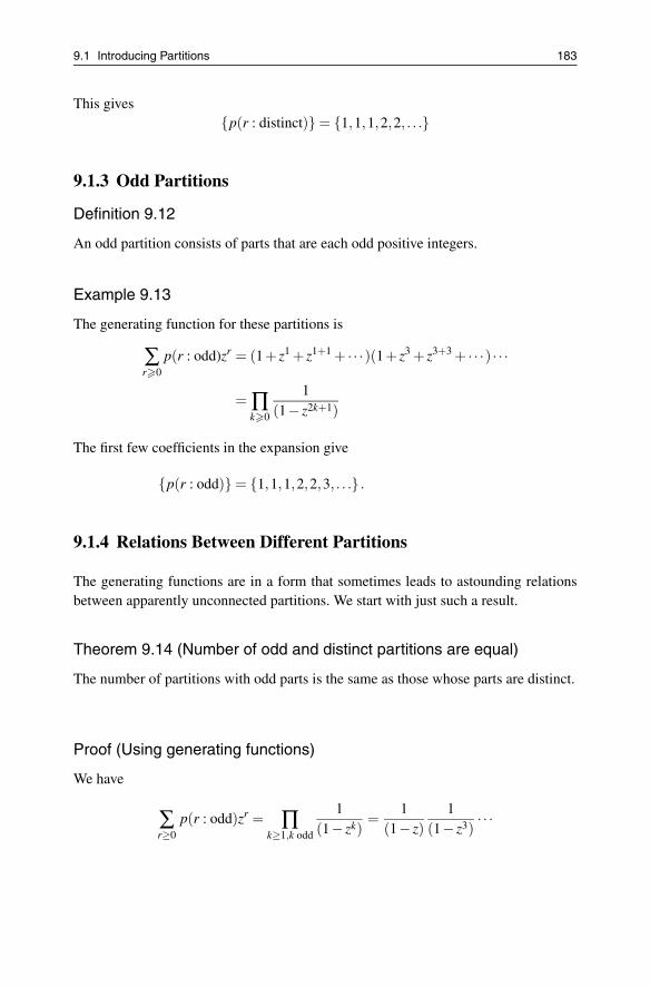
9.1 Introducing Partitions 183
This gives{p(r : distinct)} = {1,1,1,2,2, . . .}
9.1.3 Odd Partitions
Definition 9.12
An odd partition consists of parts that are each odd positive integers.
Example 9.13
The generating function for these partitions is
∑r�0
p(r : odd)zr = (1+ z1 + z1+1 + · · ·)(1+ z3 + z3+3 + · · ·) · · ·
= ∏k�0
1(1− z2k+1)
The first few coefficients in the expansion give
{p(r : odd)} = {1,1,1,2,2,3, . . .} .
9.1.4 Relations Between Different Partitions
The generating functions are in a form that sometimes leads to astounding relationsbetween apparently unconnected partitions. We start with just such a result.
Theorem 9.14 (Number of odd and distinct partitions are equal)
The number of partitions with odd parts is the same as those whose parts are distinct.
Proof (Using generating functions)
We have
∑r≥0
p(r : odd)zr = ∏k≥1,k odd
1(1− zk)
=1
(1− z)1
(1− z3)· · ·

184 9. Partitions and Paths
=1
(1− z)1− z2
(1− z2)1
(1− z3)1− z4
(1− z4)· · ·
=
(1− z2
)(1− z)
(1− z4
)(1− z2)
(1− z6
)(1− z3)
· · · = (1+ z)(1+ z2)(
1+ z3) · · ·= ∑
r≥0
p(r : distinct)zr.
Many partition identities are discovered through generating functions, but thereis a certain satisfaction in seeing an enumerative proof of the same result. It oftenprovides better insight into how the particular partitions work. So now we give another(enumerative) proof of the same result.
Proof (Using an enumerative argument)
We use two constructions: the first (Figure 9.3) reduces an odd partition to a uniquedistinct partition. The second (Figure 9.4) works in reverse. They each exploit the factthat a positive integer can always be written uniquely as the product of a power of 2and an odd number.
Figure 9.3 Odd partition to distinct partition.
Figure 9.4 Distinct partition to odd partition.
The construction creates a bijection between the two types of partition and hence

9.1 Introducing Partitions 185
there is an equal number of each.
One more result.
Theorem 9.15
The number of partitions into parts not divisible by 3 is equal to the number of parti-tions in which each part appears at most twice.
Proof
The generating function of the partitions whose parts are not divisible by 3 is:
∑r≥0
p(r : not mult. of 3)zr = ∏k≥1
k �=3l
1(1− zk)
=1
(1− z)1
(1− z2)1
(1− z4)· · ·
=
(1− z3
)(1− z)
(1− z6
)(1− z2)
(1− z9
)(1− z3)
· · · .
But now we can divide out each “numerator” by the “denominator” below it:
∑r≥0
p(r : not mult. of 3)zr =(1+ z+ z2)(
1+ z2 + z4)(1+ z3 + z6
)· · ·
= ∑r≥0
p(r : parts used at most, twice)zr.
9.1.5 Ferrers Diagram
At the heart of many enumerative proofs of partition identities is a diagram that is ageometric representation of a partition.
Definition 9.16 (Ferrers diagram)
Any partition may be represented by a set of dots, called a Ferrers diagram:
(i) in which each part of the partition is represented by a proportionate, horizontalrow of dots;
(ii) the diagram starts (at the top) with the largest part and proceeds downwards, partby part.

186 9. Partitions and Paths
Example 9.17
The Ferrers diagram for the partition 23 = 7+6+4+4+2 is the diagram:
©© © © © © ©©© © © ©©©© ©©©© ©©©©
Using this geometric idea, it is possible to give an immediate and intuitive proof ofanother partition identity.
Theorem 9.18
The number of partitions into exactly m parts is equal to the number of partitionswhose largest part is m.
Proof
Any partition whose largest part is m has a Ferrers diagram like the representation onthe left of Figure 9.5.
Figure 9.5 Ferrers diagram under diagonal reflection.
If we reflect it through the diagonal shown, it creates another partition whose Fer-rers diagram is shown on the right. This has precisely m parts.
9.1.6 Partition Recurrences
We conclude with a recurrence for the unrestricted partitions first discovered by themathematician Euler – his so-called Pentagonal Theorem. We start with the unre-stricted partition generating function, and seek to derive a recurrence relation from the

9.1 Introducing Partitions 187
denominator of it. We have
∑r≥0
p(r)zr = ∏k≥1
1(1− zk)
⇒ ∏k≥1
(1− zk) ∑r≥0
p(r)zr = 1.
At this point, Euler began expanding the expression that would make the requiredrecurrence relation,
∏k≥1
(1− zk) = (1− z)(1− z2)(
1− z3) · · ·= 1− z− z2 + z5 + z7 − z12 − z15 + z22 + z26 − z35 −·· · .
And this is where Euler made a decisive discovery. Not only were the coefficients0,1 or −1, but the powers of z with non-zero coefficients come in pairs that on eachoccurrence are one further apart, with the first power in each such pair being a termof a sequence that Euler knew only too well: {1,5,12,22,35, . . .} – the Pentagonal
sequence of numbers{
r(3r−1)2
}, so called because they can be arranged as dot patterns
of pentagons. So Euler believed that(1+ ∑
r≥1
(−1)r[
zr(3r−1)
2 + zr(3r+1)
2
])(∑r≥0
p(r)zr
)= 1
and with this result, he could derive a powerful recurrence relation to calculate suc-cessive partition numbers.
Theorem 9.19 (Euler’s Pentagonal Recurrence)
This states that
p(r) = ∑k≥1
(−1)k−1(
p(r− k(3k−1)2 )+ p(r− k(3k+1)
2 ))
for r ≥ 1
that is
p(r) = p(r−1)+ p(r−2)− p(r−5)− p(r−7)+ · · · .
We shall not prove this crucial result. Using it we find that
p(6) = p(5)+ p(4)− p(1) = 7+5−1 = 11;
p(7) = p(6)+ p(5)− p(2)− p(0) = 11+7−2−1 = 15;
. . .
p(10) = p(9)+ p(8)− p(5)− p(3) = 30+22−7−3 = 42;
p(11) = p(10)+ p(9)− p(6)− p(4) = 42+30−11−5 = 56.

188 9. Partitions and Paths
It is possible to continue in this way and use the recurrence to find values of p(r) toany designated limit. For example, great perseverance gives
p(10) = 42
p(25) = 1,958
p(100) = 190,569,292
p(200) = 3,972,999,029,388.
For a discussion of this result and several proofs see [2, §14.4 & §14.5].Clearly the partition function grows, but it does so in a very complicated fashion.
There is another recurrence for the (unrestricted) partition numbers – this time we usecalculus to establish it. Again there are two proofs – one that is based on generatingfunctions and the other on enumeration. This uses a number theoretic function σ1(r),which returns the sum of the divisors of its argument.
Theorem 9.20 (The divisor/partition recurrence)
We have:
rp(r) =r
∑k=1
σ1(k)p(r− k).
Proof (Using generating functions)
We have
P(z) = ∑r≥0
p(r)zr = ∏k≥1
1(1− zk)
and taking logarithms of both sides gives
log(P(z)) = ∑k≥1
log(1− zk)−1
= ∑k≥1
∑l≥1
zkl
l;
next we use the Euler operator (zD), which gives
zP′(z)P(z)
= ∑k≥1
∑l≥1
kzkl = ∑r≥1
⎛⎜⎝ ∑
m≥1m divides r
m
⎞⎟⎠zr
= ∑r≥1
σ1(r)zr

9.1 Introducing Partitions 189
where σ1(r) is the sum of the divisors function. Rearranging this we have
zP′(z) = P(z) ∑r≥0
σ1(r)zr
and then comparing coefficients of zr on either side gives the required recurrence.
Example 9.21
We may use this recurrence to find p(6). Using the recurrence, we have
6p(6) = σ1(1)p5 + · · ·+σ1(6)p0
= 66
⇒ p(6) = 11.
This recurrence is not as efficient as Euler’s Pentagonal recurrence; its significanceis more that it relates partitions with the divisor function – two major functions ofdifferent branches of number theory.
Proof (Divisor/partition recurrence by enumeration)
First we add up all the partitions of r. There are p(r) of them, so their sum is just
rp(r).
On the other hand, consider how many times the part n appears in these partitions.It appears at least once in p(r − n) partitions; it appears at least twice in p(r − 2n)partitions; and so on. The total number of times it appears is ∑q p(r−qn). We musthave
rp(r) =r
∑n=1
n∑q
p(r−qn) = ∑qn≤r
np(r−qn) =r
∑k=1
p(r− k)∑q|k
q
=r
∑k=1
p(r− k)σ1(k)
exactly as required.
9.1.7 Exercises
Exercise 9.1
Interpret the infinite product
P(z) = (1+ z+ · · ·+ z9)(1+ z10 + · · ·+ z90)(1+ z100 + · · ·+ z900) · · ·
as a partition generating function and so write down its expansion.

190 9. Partitions and Paths
Exercise 9.2
Prove that the number of partitions in which each part appears at most fourtimes is equal to the number of partitions into parts which are not divisible by5.
Exercise 9.3
Find the generating function corresponding to the partitions in which:
(i) the largest part is 5;
(ii) the smallest part is 5;
(iii) each part is a power of 5.
Exercise 9.4
Prove that the number of partitions in which each part appears at least twice isequal to the number of partitions whose parts (mod 6) are not congruent to±1.
Exercise 9.5
If p(r : parts ≤ k) is the number of partitions in which the parts are no largerthan k, establish the recurrence (using enumerative and generating functionarguments)
p(r : parts ≤ k) = p(r : parts ≤ k−1)+ p(r− k : parts ≤ k).
Exercise 9.6
Consider the partitions whose parts are powers of 3, with no power used morethan eight times. Denote the number of such partitions of r by q(r). Show thatthey satisfy the recurrence q(r) = q(r−1)+q(r−3)−q(r−4).
Exercise 9.7
Suppose that p(r : k distinct parts) is the number of partitions in which thereare k distinct parts. Using an enumerative argument, show that
p(r : k distinct parts) = p(r−k : k−1 distinct parts)+ p(r−k : k distinct parts).
Exercise 9.8
Show that p(r : odd parts) is
r
∑k=0
p(k : distinct odd parts)p(r− k : even number of odd parts).

9.2 Triangular Partitions of a Polygon 191
Exercise 9.9
Show that
p(r : distinct parts) = p(r−1 : distinct parts)+ p(r : distinct, not power of 2).
Exercise 9.10
Determine p(r : {1,2,22, . . .}).
9.2 Triangular Partitions of a Polygon
In 1751 Euler posed this problem to his fellow mathematician Goldbach: find thenumber of ways to partition a convex, plane polygon with r sides into triangles whosesides join vertices of the polygon and do not intersect. Goldbach, of course, may havebeen tied up with a number of competing conjectures; whatever, he seems not to havemade any progress with the problem. But Euler did. He realized that if the polygonwas convex, then the enumeration of these triangular partitions depended only on thenumber of sides of the polygon. We take this as a given. Euler had also found resultsfor all such polygons with nine or fewer sides. He discovered that a triangle has onlyone such triangulation: itself. For a square it is almost as easy – there are just two waysto triangulate it. For a pentagon, things start to get complicated since there are fiveways to triangulate it (Figure 9.6). Notice that some of these partitions are essentially
Figure 9.6 Triangular partitions of a pentagon.
the same if we are thinking geometrically – there are symmetries that map one intoanother, as in Chapter 6. However, here we are really dealing with a labelled diagramand each such partition is then distinct. Moving on to a hexagon in the same spirit,there are fourteen triangulations of a (regular) hexagon. Euler had soon developed theformula
2.6.10 · · ·(4r−10)(r−1)!

192 9. Partitions and Paths
for the number of such partitions, but was unable to prove it. This was no simpleoversight on Euler’s part. Despite its simple appearance, the problem is very difficult,and Euler’s conjectured formula confirms that fact. The next step forward was madeby another mathematician, Segner. Euler had sent on his first seven triangular parti-tion numbers and Segner had responded with a recurrence relation. But one of a verystrange and convoluted kind.
Definition 9.22 (Triangular partition numbers)
We call the number of triangular partitions of a convex polygon Pr with r sides, Tr.
Theorem 9.23 (Recurrence for triangular partitions)
The triangular partition numbers satisfy the recurrence
Tr =
⎧⎪⎪⎪⎨⎪⎪⎪⎩
0 : r = 0, 1;
1 : r = 2;r−1∑
k=0TkTr−k+1 : otherwise.
Proof
Consider a polygon with r sides, and one of its vertices – say the kth vertex, as shownin Figure 9.7.
Figure 9.7 Triangular partitions of a convex polygon.
We form a triangle out of the three vertices, 1, k and r. To the left of this triangle isa (proper) convex, plane polygon with k vertices, denoted Pk; to the right is one withr +1− k vertices, denoted Pr−k+1. So the number of distinct triangular partitions is
#(Pk) .1.#(Pr−k+1) = TkTr−k+1
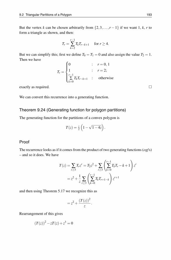
9.2 Triangular Partitions of a Polygon 193
But the vertex k can be chosen arbitrarily from {2,3, . . . ,r− 1} if we want 1, k, r toform a triangle as shown, and then:
Tr =r−1
∑k=2
TkTr−k+1 for r ≥ 4.
But we can simplify this; first we define T0 = T1 = 0 and also assign the value T2 = 1.Then we have
Tr =
⎧⎪⎪⎪⎨⎪⎪⎪⎩
0 : r = 0, 1
1 : r = 2;r−1∑
k=0TkTr−k+1 : otherwise
exactly as required.
We can convert this recurrence into a generating function.
Theorem 9.24 (Generating function for polygon partitions)
The generating function for the partitions of a convex polygon is
T (z) = z2
(1−
√1−4z
).
Proof
The recurrence looks as if it comes from the product of two generating functions (ogf s)– and so it does. We have
T (z) = ∑r≥3
Trzr = T2z2 + ∑
r≥3
(r−1
∑k=0
TkTr − k +1
)zr
= z2 +1z ∑
r≥3
(r−1
∑k=0
TkTr+1−k
)zr+1
and then using Theorem 5.17 we recognize this as
= z2 +(T (z))2
z.
Rearrangement of this gives
(T (z))2 − zT (z)+ z3 = 0

194 9. Partitions and Paths
which is a quadratic for the generating function T (z). Solving it we find that
T (z) =z2
(1−
√1−4z
).
You will be asked to check in the exercises that the negative value of the square rootis the correct choice. Expanding this generating function establishes Euler’s formula.
Corollary 9.25
The explicit forms for the number of triangular partitions of a convex polygon of rsides (for r ≥ 3) are
(i) Tr = 2r−21.3.···(2r−5)(r−1)!
(ii) Tr = 1r−1
(2r−4r−2
).
You will be asked to prove these in the exercises.The sequence of triangular partitions of a convex polygon {Tr} has the initial terms
{0,0,1,1,2,5,14,42,132, . . .}.
9.2.1 Exercises
Exercise 9.11
Given that T0 = T1 = 0 and T2 = 1, use the recurrence of Theorem 9.23 to findthe next three terms of the sequence {Tr}.
Exercise 9.12
The generating function z2
(1+
√1−4z
)is expanded. Find the first four terms
in its power series expansion.
Exercise 9.13
By expanding the generating function of Theorem 9.24, establish the explicitforms given in Corollary 9.25.
9.3 Paths in a Lattice Plane
Consider a starting point (the origin (0,0)) in a lattice made up from the positive integerpoints. We will investigate the number of paths there are when we move according to
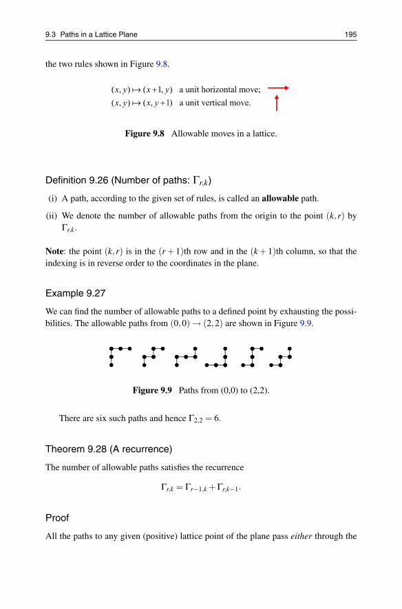
9.3 Paths in a Lattice Plane 195
the two rules shown in Figure 9.8.
Figure 9.8 Allowable moves in a lattice.
Definition 9.26 (Number of paths: Γr,k)
(i) A path, according to the given set of rules, is called an allowable path.
(ii) We denote the number of allowable paths from the origin to the point (k,r) byΓr,k.
Note: the point (k,r) is in the (r + 1)th row and in the (k + 1)th column, so that theindexing is in reverse order to the coordinates in the plane.
Example 9.27
We can find the number of allowable paths to a defined point by exhausting the possi-bilities. The allowable paths from (0,0) → (2,2) are shown in Figure 9.9.
Figure 9.9 Paths from (0,0) to (2,2).
There are six such paths and hence Γ2,2 = 6.
Theorem 9.28 (A recurrence)
The number of allowable paths satisfies the recurrence
Γr,k = Γr−1,k +Γr,k−1.
Proof
All the paths to any given (positive) lattice point of the plane pass either through the

196 9. Partitions and Paths
point below it, or the point to its left, as shown in Figure 9.10. This means that therequired recurrence is
Γr,k = Γr−1,k +Γr,k−1.
Figure 9.10 Paths from adjacent points.
Definition 9.29 (The path array)
The array (Γr,k : r,k ≥ 0) is called the path array of the allowable moves.
Using the recurrence it is easy to find the number of paths at each point by “creeping”through the lattice to obtain the initial terms in the path array, as shown in Figure 9.11.
Figure 9.11 Initial terms in the array.
Given the initial conditions and the recurrence it follows that the number of pathsarray has terms from Pascal’s triangle. We have the following result.

9.3 Paths in a Lattice Plane 197
Theorem 9.30 (Explicit form for the terms of the path array)
The number of allowable paths is given by
Γr,k =(
r + kk
).
There is an interesting enumerative argument that proves this result.
Proof
To move to the point (k,r) requires r+k moves altogether; k of these must be horizon-
tal and we immediately have Γr,k =(r+k
k
). Of course, we could equally have chosen to
consider the number of vertical moves – it leads to the same result
Γr,k =(
r + kr
)=
(r + k
k
).
9.3.1 Central Binomial Coefficients
If we consider the number of paths, Γr,r, there are to each (positive) lattice point onthe main diagonal we find an interesting result. Using Theorem 9.30 we can give theseterms an explicit form.
Corollary 9.31 (Paths to the main diagonal)
The number of allowable paths to the main diagonal is
Γr,r =(
r + rr
)=
(2rr
).
Note: the terms here are the central (even rows) Binomial coefficients. Considerationof such paths leads to another enumerative identity.
Theorem 9.32
The central Binomial coefficients are given by:
(2rr
)= ∑
k≥0
(rk
)2
.
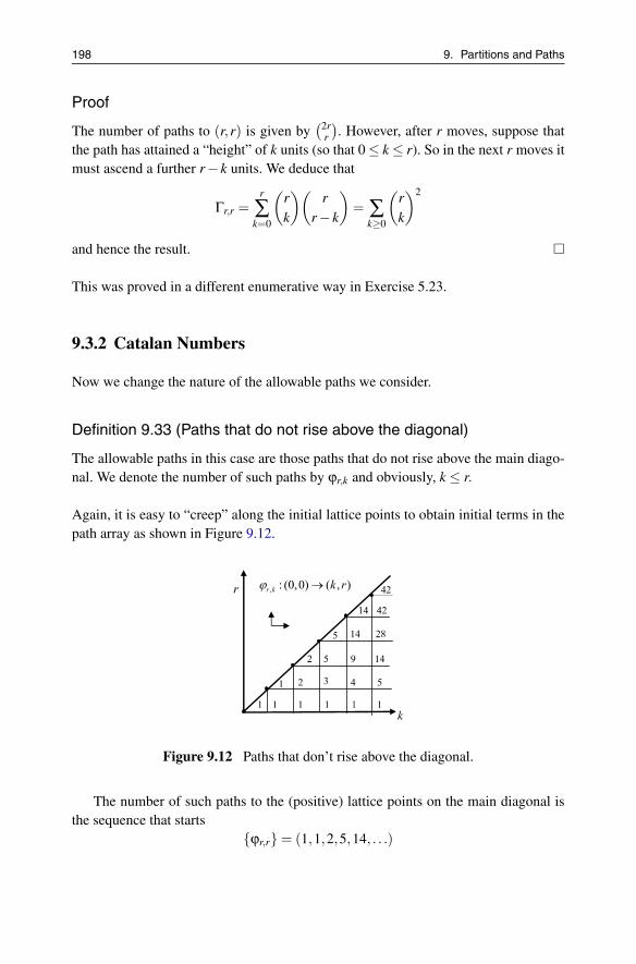
198 9. Partitions and Paths
Proof
The number of paths to (r,r) is given by(2r
r
). However, after r moves, suppose that
the path has attained a “height” of k units (so that 0 ≤ k ≤ r). So in the next r moves itmust ascend a further r− k units. We deduce that
Γr,r =r
∑k=0
(rk
)(r
r− k
)= ∑
k≥0
(rk
)2
and hence the result.
This was proved in a different enumerative way in Exercise 5.23.
9.3.2 Catalan Numbers
Now we change the nature of the allowable paths we consider.
Definition 9.33 (Paths that do not rise above the diagonal)
The allowable paths in this case are those paths that do not rise above the main diago-nal. We denote the number of such paths by ϕr,k and obviously, k ≤ r.
Again, it is easy to “creep” along the initial lattice points to obtain initial terms in thepath array as shown in Figure 9.12.
Figure 9.12 Paths that don’t rise above the diagonal.
The number of such paths to the (positive) lattice points on the main diagonal isthe sequence that starts
{ϕr,r} = (1,1,2,5,14, . . .)

9.3 Paths in a Lattice Plane 199
They appear, astonishingly, to be the Triangular partition numbers of the last section– slightly shifted. This celebrated sequence, called the Catalan numbers, is namedafter the mathematician who first investigated their properties. To show that thesevery different enumerative problems (triangular partitions and lattice paths not risingabove the diagonal) are essentially the same, we first prove two preliminary results inthe form of lemmas.
Lemma 9.34
The number of allowable paths from (0,0) to (r,r) that do not touch the main diagonaluntil (r,r) is denoted by ur. Then
ur =
{1 : r = 0;
ϕr−1,r−1 : otherwise.
Proof
Such a path (for r ≥ 1) must start with a horizontal move and finish with a verticalmove. In between, it can take any path in the shaded triangle (of Figure 9.13) thatdoes not rise above the “hypotenuse” of the triangle.
Figure 9.13 Paths that don’t meet the diagonal.
There are precisely ϕr−1,r−1 such paths inside the shaded triangle, as required.
Now we state and prove another result: in fact the terms of the Catalan sequenceare just the triangle partition numbers suitably displaced. We do so by showing thatthey obey the same recurrence and share (essentially) the same initial terms.

200 9. Partitions and Paths
Lemma 9.35
The Catalan sequence (ϕr,r) that counts the number of paths that do not meet the maindiagonal before ending on it is related to the triangular partitions of a convex polygon(Tr) by
ϕr,r = Tr+2.
Proof
Any path that goes from (0,0) to (r,r) and does not rise above the main diagonalmeets one of the points (0,0) or (1,1) or . . . or (r − 1,r − 1) or (r,r) first. Supposethat it meets (first) the point (k,k) on the diagonal, as shown in Figure 9.14.
Figure 9.14 First point it meets on the diagonal.
The number of paths from (0,0) to (k,k) that do not touch the main diagonal is(by Lemma 9.34) ϕk−1,k−1. The number of paths from (k,k) to (r,r) that do not riseabove the main diagonal is ϕr−k,r−k. So in all, the number of paths from (0,0) to (r,r)that touch the main diagonal (first) at (k,k) is
ϕk−1,k−1ϕr−k,r−k.
It now follows that
ϕr,r =r
∑k=1
ϕk−1,k−1ϕr−k,r−k
and this is the same recurrence as that for the triangular partitions of a convex polygonwith the initial conditions that ϕ0,0 = ϕ1,1 = 1.
With this relation between the triangular partitions {Tr} and the Catalan numbers{ϕr,r} we can derive other properties of the latter.

9.3 Paths in a Lattice Plane 201
Theorem 9.36
We have:
(i) the explicit form for the terms of the Catalan sequence is
ϕr,r =1
r +1
(2rr
)
(ii) its generating function is
∑r≥0
φr,rzr =
1−√
1−4z2z
.
Proof
We have from Lemma 9.35 and Corollary 9.25
ϕr,r = Tr+2 =1
r +2−1
(2(r +2−2)
r +2−2
)=
1r +1
(2rr
).
Then:
∑r≥0
ϕr,rzr = ∑
r≥0
Tr+2zr =1z2 ∑
r≥0
Tr+2zr+2 =1z2 ∑
r≥0
Trzr
and hence
∑r≥0
ϕr,rzr =
1−√
1−4z2z
.
The Catalan sequence is usually written {Cr} and has the initial terms
{Cr} = {1,1,2,5,14, . . .}.
9.3.3 Exercises
Exercise 9.14
Catalan first discovered the sequence of numbers that bear his name, {Cr},when he investigated the problem of determining the number of ways that a listof r + 1 terms {α0,α1, . . . ,αr} could be bracketed so that the order of multi-plication is completely specified. For example, the number C2 is the number ofways to bracket {α0,α1,α2} and it is #{(α0)(α1,α2),(α0,α1)(α2)} = 2. Wealso have C3 = 5. Construct a recurrence for this sequence.

202 9. Partitions and Paths
Exercise 9.15
By simplifying the expression(2r
r
)−
( 2rr+1
)show that the Catalan number for-
mula, Cr = 1r+1
(2rr
), does yield integers.
Exercise 9.16
Find the generating function of the Catalan numbers from the generating func-tion
∑r≥0
(2rr
)zr =
1√1−4z
.
Exercise 9.17
Show that the Catalan numbers have the nice summation property that
∑r≥0
Cr
4r = 2.
9.4 Miscellaneous Exercises
Exercise 9.18
Show that(1+ z+ z2
)(1+ z3 + z6
)(1+ z9 + z18
)· · · = 1
1−z .
Exercise 9.19
Consider the number of partitions of r, q(r), whose parts are powers of 3, withno power used more than eight times. You were invited to establish a recurrencein Exercise 9.6. Now use partial fractions to derive an explicit form for q(r).
Exercise 9.20
Find an explicit form for the number of partitions of r which consist of powersof 2, where no power can be used more than three times.
Exercise 9.21
Show that the number of partitions with no parts equal to 3, q(r), is related tounrestricted partitions by q(r)+ p(r−3) = p(r).
Exercise 9.22
The divisor/partition recurrence (Theorem 9.20)
rp(r) =r
∑k=1
σ1(k)p(r− k)

9.4 Miscellaneous Exercises 203
may be written in matrix form. Use the initial terms of this matrix, show that⎛⎜⎜⎜⎜⎜⎝
σ1(1)σ1(2)σ1(3)σ1(4)
.
⎞⎟⎟⎟⎟⎟⎠
=
⎛⎜⎜⎜⎜⎜⎝
1−1 1 .
−1 −1 1 .
0 −1 −1 1 .
. . . . .
⎞⎟⎟⎟⎟⎟⎠
⎛⎜⎜⎜⎜⎜⎝
1p(1)2p(2)3p(3)4p(4)
.
⎞⎟⎟⎟⎟⎟⎠
.
Exercise 9.23
Show that the number of paths to (r,r) that rise above the diagonal is( 2r
r−1
).
Exercise 9.24
How many “mountain ranges” can be formed with r upstrokes and r down-strokes? An example is shown in Figure 9.15.
Figure 9.15 “Mountain ranges”.
Exercise 9.25
Prove that the Catalan numbers have the product form
Cr =1
(r +1)!
r
∏k=1
(4k−2).
Exercise 9.26
Derive the identity
∑k≥0
(2kk
)(2r−2kr−2
)= 4r.

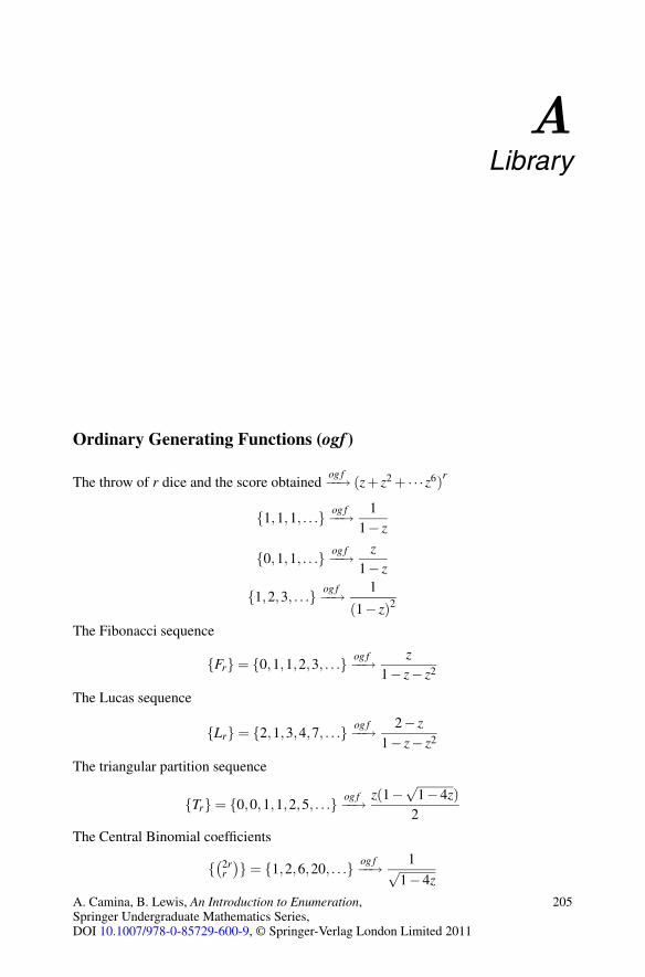
ALibrary
Ordinary Generating Functions (ogf )
The throw of r dice and the score obtainedog f−−→ (z+ z2 + · · ·z6)r
{1,1,1, . . .} og f−−→ 11− z
{0,1,1, . . .} og f−−→ z1− z
{1,2,3, . . .} og f−−→ 1
(1− z)2
The Fibonacci sequence
{Fr} = {0,1,1,2,3, . . .} og f−−→ z1− z− z2
The Lucas sequence
{Lr} = {2,1,3,4,7, . . .} og f−−→ 2− z1− z− z2
The triangular partition sequence
{Tr} = {0,0,1,1,2,5, . . .} og f−−→ z(1−√
1−4z)2
The Central Binomial coefficients
{(2r
r
)} = {1,2,6,20, . . .} og f−−→ 1√
1−4z
A. Camina, B. Lewis, An Introduction to Enumeration,Springer Undergraduate Mathematics Series,DOI 10.1007/978-0-85729-600-9, © Springer-Verlag London Limited 2011
205

206 A. Library
The Catalan sequence
{Cr} = {1,1,2,5,14, . . .} og f−−→(1−
√1−4z
)2z
Unrestricted partitions
{p(r)} = {1,1,2,3,5, . . .} og f−−→ 1(1− z)(1− z2)(1− z3) · · ·
Partitions whose parts are distinct
{p(r : distinct)} = {1,1,1,2,2,3, . . .} og f−−→ (1+ z)(1+ z2)(1+ z3) · · ·
Partitions whose parts are odd
{p(r : odd)} = {1,1,1,2,2,3, . . .} og f−−→ 1(1− z)(1− z3)(1− z5) · · ·
Exponential Generating Functions (egf )
{ur} = {1,1,1, . . .} eg f−−→ ez
The Fibonacci sequence
{Fr} = {0,1,1,2,3, . . .} eg f−−→ 1√5
(eφ1z − eφ2z)
The Lucas sequence
{Lr} = {2,1,3,4,7, . . .} eg f−−→ eφ1z + eφ2z
The Derangement sequence
{dr} = {1,0,1,2,9, . . .} eg f−−→ e−z
1− z
The push-button lock sequence
{cr} = {1,2,5,16,65, . . .} eg f−−→ ez
1− z
Involutions – permutations all of whose cycles are of length 2 or less
{σ(r : cycles ≤ 2} = {1,1,2,4,10, . . .} eg f−−→ ez+ z2
2
Permutations all of whose cycles are of length 2
{σ(r : cycles =2} = {1,0,1,0,3,0, . . .} eg f−−→ ez2
2
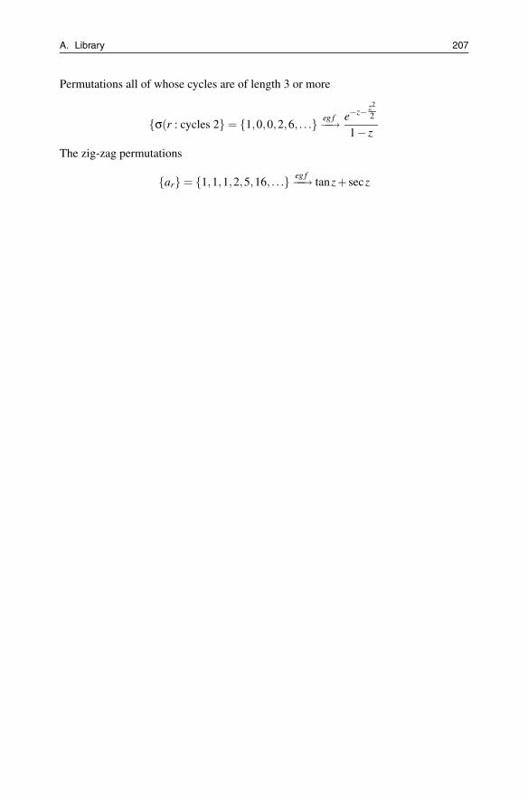
A. Library 207
Permutations all of whose cycles are of length 3 or more
{σ(r : cycles 2} = {1,0,0,2,6, . . .} eg f−−→ e−z− z2
2
1− z
The zig-zag permutations
{ar} = {1,1,1,2,5,16, . . .} eg f−−→ tanz+ secz


Solutions
Chapter 1
1.1(r
k
)counts the number of ways to select k from r, which also counts selecting r−k
from r, since they are selected by not being selected.
1.2 We can choose one from each r, r and r in ((r
1
))3 ways. We can choose two from
one r, one from another r and none from the final r in(r
2
)(r1
)ways and there are six
ways of doing this. We can choose three from one r and none from the others in(r
3
)ways. There are three possible ways to do this. The result follows.
1.3 Thirteen socks.
1.4 Seven times.
1.5 (i) Split up the unit equilateral triangle into four equilateral triangles with sides12 . If five points are placed in the triangle, then at least two of them must be in oneof the smaller triangles – and must be separated by less than 1
2 . (ii) Split up the unitequilateral triangle into nine equilateral triangles with sides 1
3 . So 10 points placedinside must be less that 1
3 apart.
1.6 Of two consecutive integers, one of them is divisible by 2; of three consecutiveintegers, one of them is divisible by 3; etc.
1.7 The number is 6300− (2100+1575+1260)+(525+420+315)−105 = 2520.
1.8 (i) 2 is fixed in 3! ways. So 4!− 3! = 18 counts the number of ways that 2 is notfixed. (ii) 2 and 4 are fixed in 2! ways. So 4!− (3!+3!)+2! = 14 counts the numberof ways that 2 and 4 are not fixed.
1.9 The number of integers relatively prime to r is r(1− 1p1
)(1− 1p2
).
1.10 Consider three cases when x is: an integer; has fractional part < 12 ; has fractional
A. Camina, B. Lewis, An Introduction to Enumeration,Springer Undergraduate Mathematics Series,DOI 10.1007/978-0-85729-600-9, © Springer-Verlag London Limited 2011
209

210 An Introduction to Enumeration
part ≥ 12 .
1.11 To choose k from r + l we can choose m from r and k−m from l for 0 ≤ m ≤ k.
1.12 24 = b4 + 6.1 + 3.1, which gives b4 = 15; 5! = b5 +(5
2
)b3 + 1
2!
(52
)(32
)b1 which
gives b5 = 75.
Chapter 2
2.1 The generating function is easily seen to be (z + z2 + · · ·+ z6)10, which becomesz10(1− z6)10(1− z)−10. We require the coefficient of z25, which is
(100
)(2415
)−
(101
)(189
)+
(102
)(123
).
2.2 From Example 2.7 the answer is 676.
2.3 The generating function is ∑r≥0 urzr = 1(1−z)(1−z3) and using partial fractions this
is 13
(1
1−z + 1(1−z)2 + 1−z2
1−z3
). So the required coefficient is 1
3 (1+201−1) = 67. An
alternative approach is to consider how many 3p coins will be used, so the answer is�(200/3)� = 67.
2.4 1, p1 and p21 are the divisors of p2
1 and 1, p2, p22 and p3
2 are the divisors of p32 and
hence the result.
2.5 Consider a legal expression of length r. It must either end in a double digit or inan operation followed by a digit. In the first case we may add another digit to one ofthe ar−1 legal expressions in 10ar−1 ways. In the second case, from one of the ar−2
legal expressions we can add 29 combinations of an operation and a digit – excludingdivision by zero. So ar = 10ar−1 +29ar−2.
2.6 A legal string of length r either starts with a 0 and must then be followed by a1 and a legal string of length r− 2, or it starts with a 1 and can be followed by anylegal string of length r−1. Hence ur = ur−2 +ur−1 and the initial conditions then giveur = Fr+2.
2.7 Consider the final summand: it is either 1 or 2. So ur+1 = ur + ur−1 and henceur = Fr+1.

Solutions 211
2.8 We have
rdr−1 = rr−1
∑k=0
(−1)k(
r−1k
)(r− k−1)! =
r−1
∑k=0
(−1)k(
rk
)(r− k)!
=r
∑k=0
(−1)k(
rk
)(r− k)!− (−1)r = dr − (−1)r
as required. We use this for consecutive values of r: dr = rdr−1 +(−1)r and dr−1 =(r−1)dr−2 +(−1)r−1 and addition gives dr +dr−1 = rdr−1 +(r−1)dr−2 so that dr =(r−1)(dr−1 +dr−2), as required.
2.9 By definition, Lr = Fr−1 + Fr +1 and so Lr + Lr+1 = Fr−1 + Fr+1 + Fr + Fr+2 =2Fr+1 +Fr+2 = Fr+1 +Fr+3 = Lr+2, as required.
2.10 (i) 11+z ; (ii) 1
(1+z)2 ; (iii) 12 ( 1
(1+z)2 + 1(1−z)2 ).
2.11 log 11−z .
2.12 4+z1−z−2z2 .
2.13 The generating function for ar is 4−4z1−2z−15z2 .
2.14 L(z)−2− z = z(L(z)−2)+ z2L(z) gives L(z) = 2−z1−z−z2 .
2.15 Either a string of length r has one or more 0s or it has no 0s. So ur+1 = 3ur +3r.The generating function is 1−2z
(1−3z)2 (which gives ur = (r +3)3r−1).
2.16 It is easy to prove (by induction) that Mr =(
Fr−1 Fr
Fr Fr+1
). The first result
easily follows from the definition of Lucas numbers. We also have |M|=−1 and hence|Mr|= (−1)r. But we can evaluate the determinant directly, and |Mr|= Fr−1Fr+1−F2
r
and the result follows.
2.17 The generating function is 1(1−z)(1−z2) = 1
4( 11−z + 1
1+z + 2(1−z)2 ). (So the required
number is 2r+3+(−1)r
4 ).
2.18 In each module, the mark is generated by (1+z+z2 + · · ·+zm). So we require the
coefficient of z3m in (1+ z+ z2 + · · ·+ zm)6. Rewrite this as (1−zm+1)6
(1−z)6 = (1−6zm+1 +
15z2m+2 + · · ·)∑s≥0(5+s
5
)zs. The required number follows.
2.19 A sum that makes r ends in a 1, a 2 or a 3. So pr = pr−1 + pr−2 + pr−3.
2.20 A tiling either ends with a configuration of tiles that takes up a single horizontalspace (one double tile placed vertically, or two single tiles placed on top of each other),or with a configuration of tiles that takes up a double horizontal space (one horizontaldouble on top of two singles; or reverse this; or two doubles on top of each other).This gives the required recurrence. The generating function is 1
1−2z−3z2 with f0 = 1and f1 = 2.

212 An Introduction to Enumeration
Chapter 3
3.1 vr = 4r +3.4r−1 = 7.4r−1.
3.2 For example, (1+√
5)3−(1−√
5)3
23.√
5= 2 = F3.
3.3 If (1− 3z + z2) = (1− θ1z)(1− θ2z) then θ1 + θ2 = 3 and θ1θ2 = 1. This gives
θ1,2 = 3±√
52 . We find that ur = (3+
√5)r+(3−
√5)r
2r = (1+√
5)2r+(1−√
5)2r
22r = L2r.
3.4 This time, vr = F2r+1.
3.5 L2r = φ2r1 + φ2r
2 and so ∑r≥0 L2rzr = ∑r≥0(φ21z)r + ∑r≥0(φ2
2z)r = 11−φ2
1z+ 1
1−φ22z
= 2−(φ21+φ2
2)z1−(φ2
1+φ22)z+φ2
1φ22z2 = 2−3z
1−3z+z2 . The recurrence follows from the denominator. Simi-
larly, ∑r≥0 L3rzr = 2−4z1−4z−z2 .
3.6 ∑r≥1 urzr = 2z∑r≥1 ur−1zr−1 + 2∑r≥1(2z)r−1 + 3∑r≥1(3z)r−1 and so U(z)−1 =2zU(z) + 2
1−2z + 31−3z and so U(z) = 6−17z+6z2
(1−2z)2(1−3z) which leads to the recurrenceur = 7ur−1 −16ur−2 +12ur−3.
3.7 The characteristic equation is θ2 − 2θ + 2 = 0, which has roots θ = 1± i. Thisleads to ur =
(1−2i
2
)(1+ i)r +
(1+2i
2
)(1− i)r.
3.8 nr+1 = 3.10r + 4nr and so 10nr = 3.10r + 40nr−1. Subtraction of these givesnr+1 = 14nr − 40nr−1. This leads to nr = C4r + D10r, and the initial values deter-mined in Example 2.11 then give C = D = 1
2 .
3.9 The sequence proceeds {3,0,3,3,6,9,15, . . .} = 3{1,0,1,1,2,3,5, . . .}. We con-jecture that Gr = 3Fr−1. This is easily proved by induction.
3.10 We have ar+1 +√
3br+1 = (1 +√
3)(ar +√
3br). Multiplying out the right-hand side of this and then comparing rational and irrational parts (the sequencesar and br are each integer sequences) gives the required results. From the first ofthese we have br = ar+1−ar
3 and substituted into the second gives (when rearranged)ar+2 = 2ar+1 + 2ar. The sequence {br} satisfies the same recurrence. We then havear = 1
2 ((1+√
3)r +(1−√
3)r) and br = 12√
3((1+
√3)r − (1−
√3)r).
3.11 The recurrence, and the initial values f0 = 1 and f1 = 2, leads to the gen-erating function F(z) = 1
1−2z−3z2 . Using partial fractions and expanding then gives
fr = 3r+1+(−1)r
4 .
3.12 The generating function satisfies 1z (A(z)− 1) = 3A(z) + 2
1−2z , which becomes(using partial fractions) A(z) = 3
1−3z −2
1−2z and hence ar = 3r+1 −2r+1.
3.13 Suppose there are ur permutations of {1,2, . . . ,r} that move each element fewerthan two places. Now consider ur+1. Where does r + 1 go? It must either go in the

Solutions 213
penultimate place (in which case it must be followed by r) or it goes in the final place.So ur+1 = ur + ur−1. Using the initial conditions that u1 = 1 and u2 = 2 this meansthat ur = Fr+1.
3.14 Either a word starts with an e (which must then be followed by an a) or it doesn’t(so it starts with a or t). So wr = wr−2 + 2wr−1 and w0 = 1,w1 = 2. Using Theo-rem 3.23 this gives wr = 1
2√
2((1+
√2)r+1 − (1+
√2)r+1).
3.15 A word of length r ends in either v (so the next letter is e,r, or y); or e (so the nextletter is v, r or y); or r (so the next letter is v, e or y); or y (so the next letter is v, e orr). It follows that wr+1 = 3wr and then wr = 4.3r−1 for r ≥ 1.
3.16 We have (from Example 3.4) φ1 +φ2 = 1 and multiplication by φ1 gives φ21 −1 =
φ1; hence the required result. (φ1 and φ2 are always interchangeable.) If we multiplythe result again by φ1 we find φ2
1 = 2φ1 +1. Induction proves the remaining result.
3.17 (i) These polynomials follow readily from the given recurrence. (ii) As the inde-terminate “w” is independent of r, we may construct the given characteristic equation
as given. (iii) Solving the characteristic equation gives θ1,2 = w±√
w2+42 and this leads
to the given explicit form of the polynomials.
3.18 If the denominator and numerator of the generating function of the sequence {ur}are, respectively, a0 +a1z+ · · ·+apzp and b0 +b1z+ · · ·+bqzq then(∑p
t=0 atzt)
∑r�0 urzr = ∑qs=0 bszs and comparing coefficients of zr when r > q gives
the recurrence ∑pt=0 atut = 0.
3.19 The given expression is (using partial fractions) 1 + 1(1−z)2 −
11−z and then com-
paring coefficients gives ur −ur−6 = (r +1)−1 for r ≥ 7.
Chapter 4
4.1 Let Hi be a family of subgroups of G indexed by a set I. Let ∩i∈IHi = H. Letx,y ∈ H. Then x,y ∈ Hi for all i ∈ I. By the properties of subgroups we have that xyand x−1 are both in Hi for all i ∈ I, so both are in H. So H is a subgroup of G. Now forany subset X consider the family of subgroups which contain X . This is not empty asG is in the family. Define 〈X〉 to be the intersection of this family. It is now clear that〈X〉 is the smallest subgroup of G containing X . This is called the subgroup generatedby X and is written 〈X〉.4.2 Consider the set {gm : m ∈Z}. Note that the number of elements in this set is n. Soamongst the set {g0,g1, . . . ,gn} there must be two elements the same. Say gi = g j for
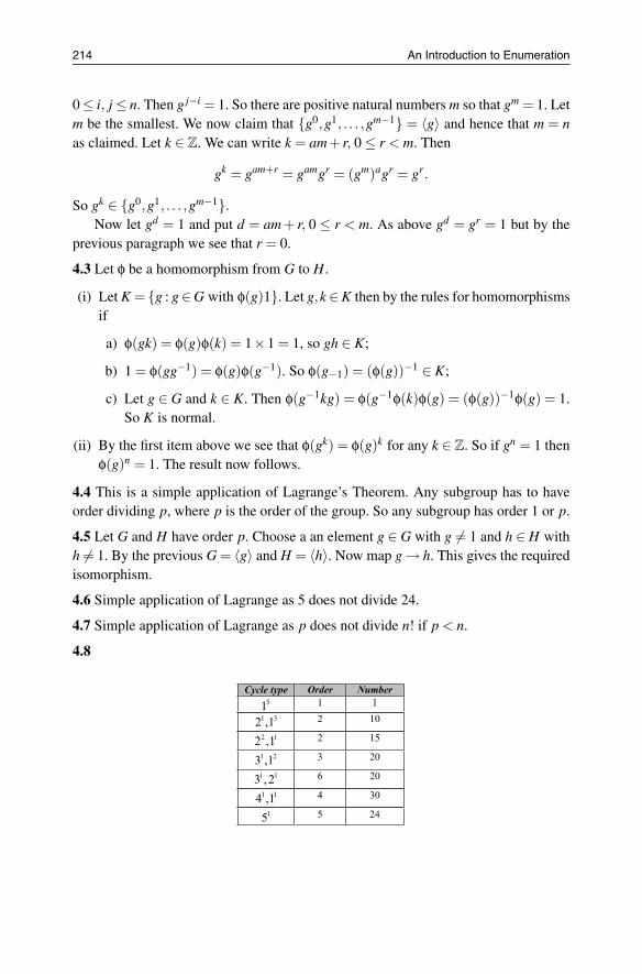
214 An Introduction to Enumeration
0 ≤ i, j ≤ n. Then gj−i = 1. So there are positive natural numbers m so that gm = 1. Letm be the smallest. We now claim that {g0,g1, . . . ,gm−1} = 〈g〉 and hence that m = nas claimed. Let k ∈ Z. We can write k = am+ r, 0 ≤ r < m. Then
gk = gam+r = gamgr = (gm)agr = gr.
So gk ∈ {g0,g1, . . . ,gm−1}.Now let gd = 1 and put d = am + r, 0 ≤ r < m. As above gd = gr = 1 but by the
previous paragraph we see that r = 0.
4.3 Let φ be a homomorphism from G to H.
(i) Let K = {g : g∈G with φ(g)1}. Let g,k ∈K then by the rules for homomorphismsif
a) φ(gk) = φ(g)φ(k) = 1×1 = 1, so gh ∈ K;
b) 1 = φ(gg−1) = φ(g)φ(g−1). So φ(g−1) = (φ(g))−1 ∈ K;
c) Let g ∈ G and k ∈ K. Then φ(g−1kg) = φ(g−1φ(k)φ(g) = (φ(g))−1φ(g) = 1.So K is normal.
(ii) By the first item above we see that φ(gk) = φ(g)k for any k ∈ Z. So if gn = 1 thenφ(g)n = 1. The result now follows.
4.4 This is a simple application of Lagrange’s Theorem. Any subgroup has to haveorder dividing p, where p is the order of the group. So any subgroup has order 1 or p.
4.5 Let G and H have order p. Choose a an element g ∈ G with g �= 1 and h ∈ H withh �= 1. By the previous G = 〈g〉 and H = 〈h〉. Now map g → h. This gives the requiredisomorphism.
4.6 Simple application of Lagrange as 5 does not divide 24.
4.7 Simple application of Lagrange as p does not divide n! if p < n.
4.8

Solutions 215
4.9 This just involves looking at the possible cycle lengths. We need a partition of10 = a+b+ c+ · · · so that lcm(a,b,c, . . .) is maximal. It is 5+3+2.
4.10 We see that the number of transpositions in the symmetric group of degree r isjust r(r−1)
2 So the ogf is given by ∑r≥2r(r−1)
2 zr so the answer is z2
(1−z)3 .
4.11 The main thing to check is that if g is a permutation there is a permutation h sothat gh = hg = the identity map. For any x ∈ X define h(x) = y where g(y) = x. Sinceg is onto there is such a y and because g is 1−1 then y is unique.
4.12 Define the action of G on subsets of G by g(X) = gX where X ⊆ G, g ∈ G. Thisis a well-defined action and the set GX = {G : gX = X} is just the stabilizer of a pointin the action.
4.13 Consider the set {gm : m ∈ Z}. Note that the number of elements in this set n. Soamongst the set {g0,g1, . . . ,gn} there must be two elements the same. Say gi = g j for0 ≤ i, j ≤ n. Then g j−i = 1. So there are positive natural numbers m so that gm = 1. Letm be the smallest. We now claim that {g0,g1, . . . ,gm−1} = 〈g〉 and hence that m = nas claimed. Let k ∈ Z. We can write k = am+ r, 0 ≤ r < m. Then
gk = gam+r = gamgr = (gm)agr = gr.
So gk ∈ {g0,g1, . . . ,gm−1}.Now let gd = 1 and put d = am + r, 0 ≤ r < m. As above gd = gr = 1 but by the
previous paragraph we see that r = 0.
4.14 We first show that it has order 24. It is clear that the action is transitive on vertices.So fix any vertex, say V , then the stabilizer of V acts on the triangle formed by theremaining vertices. So the stabilizer is isomorphic to Sym(3) and has order 6. Thereare four vertices so the stabilizer of V has index 4 in the whole group. So we haveorder 24. But clearly the whole group is inside Sym(4) as there are four vertices.
An alternative approach is geometric. Consider the various rotations that will pre-serve the tetrahedron. For example choose any vertex and the midpoint of the oppositeface, then rotate through π/3. By choosing each vertex in turn there are eight distinctelements of order 3. Then consider reflections.
4.15 The key argument is that if g and h are permutations and g has a cycle (a1a2 . . .ar)then hgh−1 has a cycle (h(a1)h(a2) . . .h(ar)).
If (b1b2 . . .br) is another cycle, consider a permutation k that has k(ai) = bi. Thenk(a1a2 . . .ar)k−1 = (b1b2 . . .br). So putting disjoint cycles together gives the result.
4.16 The subgroup that fixes X1 + X2 −X3 −X4 is {(12),(34),(12)(34)}. One suchpolynomial is X1X2 +X2X3 +X3X4 +X4X1.
4.17 An element of order p generates a cyclic group of order p. So each orbit haslength 1 or p. Since n is not divisible by p there has to be an orbit of length 1. An orbitof length 1 corresponds to a fixed point.

216 An Introduction to Enumeration
4.18 Using the definitions φ(g)φ(g−1) = φ(1). So φ(g1) = (φ(g))−1. Now it is straight-forward to show that φ is a bijection.
4.19 Using the definitions φ(g)φ(h) = φ(g)(xh−1) = xh−1g−1 = x(gh)−1 = φ(gh)(x)which is exactly what is required. The identity works correctly.
The reason for the inverse is to make the product come out correctly, without theinverse we would have φ(g)φ(h) = φ(hg).
4.20 Let x ∈ {1,2, . . . ,n}. Then start with x and keep applying g. Any element in G isof the form gm for some m ∈ N. So y is in the same orbit as x if and only if y = gk(x)for some k ∈ N.
4.21 We can use a similar argument to that used for the tetrahedron. There are sixfaces and the symmetry group, say G, acts transitively on them. Pick any face, say F ,and note that [G : GF ] = 6. The opposite face has to be fixed. Now the remaining fourfaces can be thought of as a square and so |GF | = 8. so the order is 48.
Geometrically the elements are: 9 rotations (by ±π/2 or π) about centres of 3pairs of opposite faces, 6 rotation (by π) about centres of 6 pairs of opposite edges. 8rotations (by ±2π/3) about 4 pairs of opposite vertices (diagonals). [8] Together withthe identity this accounts for all 24 elements. Then there are the reflections.
4.22 Consider the class
|G| =k
∑1|Ci|.
Divide everything through by |G| = n to get the equation
1 =1n
+n1
n+ · · ·+ nr
n.
If there are only two conjugacy classes then we have the equation
1 =1n
+kn.
So k = n−1 but k divides n so k = 1 and n = 2.If there are only three conjugacy classes then we have the equation
1 =1n
+kn
+ln.
So k + l = n−1 and both k and l divide n. We can list the possibilities:
(i) k = l = 1 and n = 3
(ii) k = 3, l = 2 and n = 6.
4.23 This is a simple application of the Orbit-Stabilizer Theorem. Since every orbithas order the index of a subgroups and such indices divide the order of the group(Lagrange’s Theorem), the result follows.

Solutions 217
4.24 For r = 2 there are just the two orbits: {(x,y) : x �= y} and {(x,x)}.For r = 3 we have the orbits given by {(x1,x2,x3) : xi all distinct}, {(x1,x1,x2) :
x1 �= x2}{(x1,x2,x1) : x1 �= x2}, {(x2,x1,x1) : x1 �= x2} and finally {(x1,x1,x1)}.The number of orbits is determined by the positions of the entries which are the
same. So we can construct a partition of r where each subset of the partition is the posi-tions where the entries are the same. So for r = 3 we have the partitions, {1},{2},{3},{1,2},{3}, {1,3},{2}, {2,3},{2} and {1,2,3}.
4.25 The first term of the sum counts how often p divides n or how many of the se-quence {1,2, . . . ,n} are divisible by p. Similarly the second term counts how often p2
divides n or how many of the sequence {1,2, . . . ,n} are divisible by p2. Adding all theterms gives how many ps divides n!, which is the order Sym(n).
4.26 We know(pam
pa
)= (mpa)!
pa!(mpa−m)! . By the previous exercise(pam
pa
)is divisible by
mpa−1 +mpa−2 + · · ·+m−(
pa−1 + pa−2 + · · ·+1)
−((m−1)pa−1 +(m−1)pa−2 + · · ·+(m−1)
)= 0.
Chapter 5
5.1 We start from the Binomial theorem slightly adapted, ∑k≥0(r
k
)zk+1 = z(1+ z)r. If
we differentiate this (wrt z) and let z = 1 the result follows.
5.2 Think of choosing a football team of k players, with a captain, from r players. Wecan choose the k from r and then 1 from the k; or we can choose 1 from r and thenk−1 from the r−1 remaining.
5.3 We may choose k from r + 1 in(r+1
k
)ways. Now consider an arbitrary element.
Either it is included in the choice, so choose the remainder k−1 from r in( r
k−1
)ways;
or it is not included, so choose k from r remaining in(r
k
)ways, and hence the result.
Three successive diagonal sums of Pascal’s triangle have each term of this recurrence,so they also obey it. As the first two sums are Fibonacci, so are they all.
5.4 Think of a committee of k members and an executive sub-committee of l members– see Exercise 5.2.
5.5 Split up r into m and r−m. We can choose 0 from m and k from r−m; or 1 fromm and k−1 from r−m; etc.
5.6 We have rcr−1 = r ∑k�0(r−1
k
)k! = ∑k�0
( rk+1
)(k + 1)! = ∑k�0
(rk
)k!− 1 = cr − 1
using Exercise 5.2. In constructing a cr from a cr−1 the “new” button r either joins anexisting combination (and it has r places to do this) or it is a combination by itself.
5.7 From the last exercise, we have cr = rcr−1 +1 and cr+1 = (r+1)cr +1. Subtracting

218 An Introduction to Enumeration
these gives the result.
5.8 The result is true for r = 1. Suppose it is true for r. Then r! = ∑k�0(−1)r−k(r
k
)ck
and hence (r +1)! = ∑k�0(−1)r−k(r +1)(r
k
)ck. So
(r +1)! = ∑k�0
(−1)r−k(
r +1k +1
)(k +1)ck = ∑
k�0
(−1)r−k(
r +1k +1
)(ck+1 −1)
= ∑k�0
(−1)r+1−k(
r +1k
)ck
and the induction is complete.
5.9 The answers appear in the following section.
5.10 In general, ∑l�0 2l−r(r
l
)2k−l
(lk
)= 2k−r ∑l�0
(rl
)(lk
)= 2k−r2r−k
(rk
)=
(rk
), so the
result is true.
5.11 The characteristic equation of the matrix P3 is (1−λ)3 = 0. Every matrix satisfiesits own characteristic equation and the result follows. In general (Pn − I)n = 0.
5.12 (i) {Br} = {1,1,2,5,15, . . .}. (ii) Use Theorem 5.12.
5.13 We have ∑r�0 (−1)rr2zr = −z+z2
(1+z)3 . If we multiply each side by 11−z then on the left
we obtain the desired sum, and on the right we have −z+z2
(1−z)(1+z)3 . Partial fractions on this
gives 1(1+z)3 − 1
(1+z)2 . It now follows that ∑nk=0(−1)kk2 = (−1)n
(n+22
)−(−1)n
(n+11
)=
(−1)n n(n+1)2 .
5.14 We have Lr+2 = φr+21 + φr+2
2 and so ∑r�0 Lr+2zr = φ21
1−φ1z + φ22
1−φ2z = L2+z1−z−z2 =
3+z1−z−z2 . (i) We have 1
1−z ∑r�0 Lrzr = 2−z(1−z)(1−z−z2) = − 1
1−z + 3+z1−z−z2 and hence the
result.(ii) So 13+z ∑r�0 Lr+2zr = 1
1−z−z2 = 1z ∑r�0 Frzr and hence the result.
5.15 See previous question. We have 11−2z ∑r�0 Lrzr = 2−z
(1−2z)(1−z−z2) = 61−2z −
4+3z1−z−z2
and hence the result.
5.16 We have z(1−z2)(1−z−z2) = 1
1−z2 ∑r�0 Frzr = 1(1−z−z2) −
12
( 11+z + 1
1−z
)and hence
the results. The corresponding Lucas results arer∑
k=0L2k+1 = L2r+2 − 2 and
r∑
k=0L2k =
L2r+1 +1.
5.17 We have(∑r�0 Frzr
)2 = 15
(1
1−φ1z −1
1−φ2z
)2= 1
5
(1
(1−φ1z)2 − 21−z−z2 + 1
(1−φ2z)2
)and hence ∑r
k=0 Fr−kFk = 15 ((r +1)Lr −2Fr+1). Similarly, ∑r
k=0 Lr−kLk = (r +1)Lr +2Fr+1.
5.18 If we use the zD operator on the generating function of the Fibonacci sequencewe obtain ∑r�0 rFrzr = z+z3
(1−z−z2)2 ; the denominator of this provides the recurrence
ur = 2ur−1 +ur−2 −2ur−3 −2ur−4.

Solutions 219
5.19 The result leads to 11+z ∑r�0 Fr+2zr = 1
1−z−z2 and hencer∑
k=0(−1)r−kFk+2 = Fr+1.
5.20 We have ∑r�0 (Lr −Fr)zr = 2(1−z)1−z−z2 and dividing each side by 1− z gives the
result. We also have 5Fr =√
5(φr1 −φr
2) = (φ1 −φ2)(φr1 −φr
2) and hence the result.
5.21 We start with Theorem 2.3: ∑nk=0 ar = an+1−1
a−1 . If we apply the Euler operator aDa
to this we obtain ∑nk=0 rar = (a−1)(n+1)an−(an+1−1)
(a−1)2 and hence the result.
5.22 (i) We have k2 = k(k−1)+ k = 2(k
2
)+
(k1
). So
n
∑k=0
k2 = 2n
∑k=0
(k2
)+
n
∑k=0
(k1
)
and by Theorem 5.3 this is
n
∑k=0
k2 = 2
(n+1
3
)+
(n+1
2
)=
n(n+1)(2n+1)6
.
(ii) We have ∑r�0 r2zr = z+z2
(1−z)3 and so multiplying each side by 1/(1− z)
n
∑k=0
k2 =(
n+23
)+
(n+1
3
)=
n(n+1)(2n+1)6
.
5.23 In choosing r from 2r we can choose k from r and r−k from r, where 0 ≤ k ≤ r.So (
2rr
)= ∑
k�0
(rk
)(r
r− k
)= ∑
k�0
(rk
)2
.
5.24 The diagonal sums operate like those in Pascal’s triangle (Exercise 5.3). The firstsum is 2 and the second 1, and hence the diagonal sums are Lucas numbers.
Chapter 6
6.1 By Theorem 6.4 we have
1 =1|G| ∑
g∈G
|Fix(g)|.
But |Fix(1)| = n where the degree of G is n. So if |Fix(g)| ≥ 1 for all g ∈ G we get|G| ≤ n+ |G|−1 which can only happen if n = 1.
6.2 Using the same equation this time we find k|G|= n = |X |. So |G| divides |X |. Note

220 An Introduction to Enumeration
that if k = 1 then |X | = |G|.6.3 The two sets of vertices {A,B,D,E} and {F,C} are both fixed. We can writethe elements as {(A)(B)(C)(D)(E)(F),(AB)(ED)(FC),(AE)(BD),(AD)(BE)(FC)}.There are two orbits on vertices as above; check using Equation (6.3), 6+2+0+0
4 = 2.There are eight edges and this time there are three orbits 8+2+2+0
4 = 3, and theyhave sizes 2, 2 and 4.
6.4 There are two orbits, each of size 4.
6.5 We again use the orbits and fixed point theorem. The only sequence that can befixed is one all of whose entries are the same. So k = np+(p−1)n
p , where k is the numberof orbits. So p|(np +(p−1)n), which gives the result.
6.6 Using the results from the solution 4.21, where we only consider the rotations, sothe group has order 24. The conclusion is that the cycle index of the group is
124
(Z6
1 +6Z21Z4 +3Z2
1Z22 +8Z2
3 +6Z32
).
Now replace Zi with 2 and get the answer 14.
6.7 The cycle index polynomial for the alternating group of degree four is 112(Z4
1 +3Z2
2 +8Z3Z1).
6.8 14 (Z6
1 +2Z32 +Z2
2Z21). So with k colours there 1
4(k6 +2k3 +k4) = 14 (k3(k +1)(k2 −
k +2)).
6.9 For vertices and faces the answer will be the same. There are four of each and thegroup acts like the symmetric group of degree 4. Using Table 4.1,
PG(Z1,Z2,Z3,Z4) =124
(Z4
1 +3Z22 +8Z3Z1 +6Z2Z2
1 +6Z4).
With two colours there are five ways and with three colours there are 15 ways.To consider the action of edges, recall that there are six edges so
PG(Z1,Z2,Z3,Z4,Z5,Z6) =1
24
(Z6
1 +3Z22Z2
1 +8Z23 +6Z2
2Z21 +6Z4Z2
).
With two colours there are 11 ways and with three colours there are 66 ways.
6.10PG(Z1,Z2,Z3,Z4,Z5,Z6) =
18
(Z6
1 +5Z22Z2
1
).
6.11 The required cyclic polynomial is:
PG(Z1,Z2,Z3) =16
(Z3
1 +2Z3 +3Z1Z2).
Now replace Zi with (Ri +Gi) to get
16
((R+G)3 +2(R3 +G3)+3(R+G)(R2 +G2)
).

Solutions 221
The total number is given by putting R + G = 1 (note that this is the same assubstituting 2 for each Zi).
To find the number with two reds is the coefficient of R2G in the above polynomial.There are only two terms which can contribute, (R+G)3 and 3(R+G)(R2 +G2), andthis gives 6
6 = 1.
6.12 We have already worked out the cycle structure (see Table 6.1). So
PG(Z1,Z2,Z3,Z4) =18
(Z4
1 +3Z22 +2Z2Z2
1 +2Z4).
Let the colours be R, G and B. Then the polynomial we need to study is
18
((R+G+B)4+3(R2+G2+B2)2+2(R2+G2+B2)(R+G+B)2+2(R4+G4+B4)
).
We are only interested in the terms which involve all the variables R, G and B. Aftersome simplification the answer emerges as 24
8 = 3.
6.13
So
PG(Z1,Z2,Z3,Z4) =124
(Z4
1 +3Z22 +8Z3Z1 +6Z2Z2
1 +6Z4).
The same as the answer for the tetrahedron on edges!The second part just doubles everything.
6.14 To do this observe that the group is of order 10. It has a rotation of order 5 andfive reflections.
6.15 Assume that G has at least two orbits. Let Z be an orbit of G such that |Z| < |X |.Let z ∈ Z and note that since Pz fixes exactly one point |Z| ≡ 1 (mod p). Now choosex ∈ X \Z. Then Px fixes no element in Z so |Z| ≡ 0 (mod p). This is a contradiction.
6.16 The non-trivial elements of the cyclic group act on itself as a p-cycle. For exampleg.gi = gi+1. So the group has the identity element and p− 1 elements which consistof a p-cycle. So
PG =1p
(Z p
1 +(p−1)Zp).
222 An Introduction to Enumeration
Now colour the group with k colours. We can do this in 1p (kp +(p−1)k) ways. This
has to be an integer.
6.17 We know from an earlier exercise that the required polynomial is:
124
(Z6
1 +6Z21Z4 +3Z2
1Z22 +8Z2
3 +6Z32
).
Now replace Zi with Ri +W i +Bi and then find the coefficient of R2W 2B2. This is 6.
Chapter 7
7.1 We require the coefficient of z4/4! in the egf (1+ z)6(1+ z+ z2/2). This is 1,020.
7.2 (i) Use Binet’s formula: ∑r≥0Lrzr
r! = ∑r≥0φr
1zr
r! +∑r≥0φr
2zr
r! = eφ1z + eφ2z. (ii) F2r =1√5
(φ2r
1 −φ2r2
)and so ∑r≥0
F2rzr
r! = 1√5
(eφ2
1z − eφ22z
).
7.3 We find A = 1, B = 3 and C = 1. So the egf is (z+3z2 + z3)ez.
7.4 The first form seems to lead nowhere; the second form leads to T ′(z)− t1 =T (z)− t0 + zT (z) and hence T ′(z) = (1 + z)T (z). This differential equation has the
solution T (z) = ez+ z22 .
7.5 Suppose the required egf is C(z); using the three-step recipe gives the differentialequation (see the second part of Example 7.8) C(z)− c0 = zC(z)+ ez − 1 and so theegf is C(z) = ez
1−z .
7.6 The two egf s are 11−z and e−z. They represent the sequences {r!} and {(−1)r}
respectively. So by the product formula, we have dr = ∑k≥0(r
k
)(r− k)!(−1)k.
7.7 We may rearrange the egf as e−z ∑r≥0trzr
r! = ez2
2 and if we expand each sidethe coefficients of odd powers of z on the right are zero. Hence so are those on theleft. Using Theorem 7.12 gives the required result. For even powers of z, we have∑k≥0(−1)k
(2rk
)tk = 1
22r .
7.8 This comes from the square of the egf of the Lucas numbers
(L(z))2 =(eφ1z + eφ2z)2
= e2φ1z +2ez + e2φ2z = L(2z)+2ez.
Then comparing coefficients of zr on each side and making use of the product formulagives the result.
7.9 The sequences whose egf s make up the product are {1} and {r!} respectively.By the product formula we now have the egf of the push-button lock sequence as thefunction ez
1−z .

Solutions 223
7.10 We write the egf as the product of two functions 1/(1− z)2 and ez. The first ofthese is the egf of the sequence {(r + 1)!} and the second is the egf of the sequence{1}. The product formula now gives the required result.
7.11 (i) Differentiating the egf gives ∑r≥0σr+1zr
r! = zez2
2 = z∑r≥0σrzr
r! and hence theresult. (ii) Now σ0,=2 = 1 and so σ2,=2 = 1.1, σ4,=2 = 1.1.3 and the result follows.
7.12 (i) From Theorem 4.17 we have σ3r,=3 = (3r)!3rr! (and zero otherwise), so
∑r≥0
σr,=3zr
r!= ∑
r≥0
(3r)!z3r
3rr!(3r)!= ∑
r≥0
z3r
3rr! = ez3
3 .
(ii) We can choose k from r and make them into three cycles in(r
k
)σk=3 ways, and
then make the remaining terms into involutions. Hence, using Theorem 7.12, we have
∑r≥0σr,≤3zr
r! =(
∑r≥0σr,=3zr
r!
)(∑r≥0
σr,≤2zr
r!
)and the result follows. In the final part,
the given function can be thought about in two ways. First it is the egf for the numberof permutations whose cycles are of length 1 or 2 or 3, and so on. In other words anypermutation. On the other hand it is also e− log(1−z) = 1
1−z which is the egf for thesequence which also counts all permutations. Reassuringly, these are the same.
7.13 Differentiating the egf twice gives ∑r≥0σr+2,=2zr
r! = (1+ z2)ez2
2 and hence the re-sult.
7.14 We have cr = ∑k≥0(r
k
)k! = r!∑r
k=01k! = r!
(∑
k≥0
1k! −∑k≥r+1
1k!
)= r!e−Qr where
|Qr| < 1r . We deduce that cr
r! = e− Qrr! → e as r → ∞.
7.15 We have r! = ∑k≥0(r
k
)σk,�=2σr−k,=2 and then using Theorem 7.12 this leads to
the result given. If we differentiate this we obtain ∑r≥0σr+1,�=2zr
r! = −ze− z2
21−z + e
− z2
2(1−z)2 =
−z∑r≥0σr,�=2zr
r! + 11−z ∑r≥0
σr,�=2zr
r! which leads to the given recurrence.
7.16 The egf for the sequence {cr} is ez
1−z = e2z(
e−z
1−z
)= e2z ∑r≥0
drzr
r! and the result
follows by Theorem 7.12.
7.17 (i) We have or+1 = ∑k≥0(r
k
)okor−k and so o2 = ∑k≥0
(1k
)oko1−k = o0o1 +o1o0 =
0;o3 = o0o2 +2o1o1 +o2o0 = 2;o4 = 0;o5 = 16; etc.(ii) Similarly, e2 = ∑k≥0
(1k
)oke1−k = o0e1 +o1e0 = 1; e3 = o0e2 +2o1e1 +o2e0 = 0;
o4 = 5; o5 = 0; etc.
7.18 (i) The (sort of) egf may be written (1 − z)∑r≥0urzr
r! = e−z
1−z = ∑r≥0drzr
r! and
the result follows. (ii) If we differentiate the given egf then ∑r≥0ur+2zr
r! = − e−z
(1−z)2 +
2 e−z
(1−z)3 = −∑r≥0ur+1zr
r! + 21−z ∑r≥0
urzr
r! and the recurrence follows. The sequence be-
gins {1,1,3,11,53, · · ·}.

224 An Introduction to Enumeration
7.19 Differentiating the egf gives
∑r≥0
σr+1,>2zr
r!= −(1+ z) ∑
r≥0
σr,>2zr
r!+
11− z ∑
r≥0
σr,>2zr
r!
and the recurrence follows.
7.20 Again, we recognize the left-hand side of this as a derivative, and the right as theproduct of two egf s. It follows that E ′(z) = O(z)E(z). This is easily integrated andgives E(z) = secz as required.
Chapter 8
8.1 Since the sum of the degrees of the vertices is even if each vertex has odd degreethen there has to be an even number of them.
8.2 We begin by observing that ∑d(v) = 2e. If d(v) ≥ 2 for all v then 2e = ∑d(v) ≥2|V |. So e > |V |, which contradicts |V | > e.
8.3 If a vertex has d(v) = 0 then it is not connected to anything.
8.4 Let (v0,e1,v2, . . . ,en,vn) be a path. We will use induction on n to get the result.Note that if n = 1 there is nothing to prove.
Assume that we have a path as above and we assume that vi = v j. If i �= 0 and j �= nthen we can just omit the section from vi to v j and have a shorter path. Then inductiongives the result.
8.5
(i) This is clear since each vertex in U can be joined to at most |W | vertices. So weget m ≤ rs.
(ii) n = r + s so we want to maximize the expression rs. This happens when r = s =n/2.
8.6 This is clear. If there were more than two components choose u,v,w in three dis-tinct components. But an edge can only join two vertices, so if e = (u,v) then thecomponent containing w is still a connected component.
8.7 If there are two components at leat one of them has ≤ r/2 vertices. A vertex insuch a component can be connected to at most r/2−1 vertices.
8.8 Let u and v be the pair whose degree sum is greater than r−1. By counting it canbe seen that any other vertex is joined to either u or v.
8.9 We must first write Menger’s Theorem in the edge form:Let Γ = (V,E) be a graph and let v and w be two connected vertices of V . Let k be the

Solutions 225
size of the smallest set F of edges with the property that v and w are not connected inΓ\F . Let l be largest number of simple paths from v to w which only have v and w incommon. Then k = l.
If we start with the set of edges F in the line graph it becomes a set of verticeswhich disconnects in the same way.
8.10 Choose and vertex of degree 1, say v. Then set the partitions according as thedistance from v is odd or even. Or simply observe that a tree has no cycles of oddlength.
8.11 Let T be a tree with n vertices. Then it has n− 1 edges, so if it has exactly twovertices of degree 1 the rest have degree 2, as ∑d(v) = 2n−2.
Let T1 and T2 be two such graphs. Choose vertices of degree 1, say u1 and u2, ofT1 and T2 respectively. These are joined to a unique vertex in their respective graphs.Then since these have degree 2 there is only one other vertex they are connected to.So proceeding in this way we construct the required isomorphism.
Note that these trees have an automorphism group of order 2.
8.12 A cycle is just a graph which is one simple closed path. To show that a graphwith all vertices of degree 2 is a simple closed path start anywhere, say v1. Choose v2
adjacent to v1 – there are only two choices. Then choose v3 to be the remaining vertexadjacent to v2. Keep going till you get to vn and then the only edge not used would bethe edge (vn,v1), and there is the simple closed path.
Such a path has an automorphism group of order 2n, so there are n!2n ways to label
it. So the egf is
∑ n!2n
× 1n!
zn =12
log(1− z).
8.13 One, and two.
8.14 Two.
8.15 We look at the table of elements of Sym(5) acting on pairs.

226 An Introduction to Enumeration
Now calculate the cycle index and substitute 2 for all indeterminates. This givesthe answer 34.
8.16 We use the equation v− e + f = 2. Every face is bounded by a cycle so if theshortest cycle has length g and every edge is the boundary of two faces, be carefulabout counting. So f g ≥ 2e. Substituting into the equation above gives the right an-swer.
8.17 Since the sum of the degrees of the vertices is twice the number of edges, if everyvertex has degree at least 6 we get 6v ≤ 2e. Also 3 f ≤ 2e, since every face has at leastthree edges in the boundary. So 12+6e = 6v+6 f ≤ 6e, which is clearly a contradic-tion.
8.18 This is again a variation on a theme. We get 3v ≤ 2e and 5 f ≤ 2e. So 30+15e =15v+15 f ≤ 16e. So e > 30 and f 60
5 = 12.
8.19 This time let Γ be the graph and Γ′ be its complement. The have the same numberof vertices, say v and if one has e edges the other has
(v2
)−e edges. Let them have f and
f ′ faces respectively. So we get the equations v−e+ f = 2 and v− ((v
2
)−e)+ f ′ = 2.
Combining this with the observation that 3 f ≤ 2e and 3 f ′ ≤ 2((v
2
)− e) gives the re-
sult, after some manipulation.
8.20 Consider the any face, say F , and assume that it has more than three vertices onits boundary. Then there are two which are not adjacent. Just join these two vertices– remember that edges do not have to be straight. The new graph will still be planar.So each face has three vertices and three edges on its boundary. So 3 f = 2e. Now useEuler’s formula and get 6 = 3v− 3e + 3 f = 3v− 3e + 2e = 3v− e. The two resultsfollow.
8.21 To say that the complement of a graph has no triangles is the same as saying thatthe graph does not have three vertices which form a null graph. Given any vertex v,consider the two subsets U and W which consist of the vertices adjacent to v and thosenot adjacent to v. One of these has to have size at least 3. If it is U and there are twoadjacent vertices in U then there is a triangle. If there are not two adjacent verticesthen U is a null graph.
We argue similarly if W has size at least three. If W contains two vertices which arenot adjacent then together with v they form a null graph. Otherwise W has a triangle.
8.22 Choose any vertex v and count the number of vertices at each distance i from v.When i = 1 this is clearly bounded by m. For i = 2 the answer is m(m− 1) and forarbitrary i the answer is m(m−1)i−1. So the bound on the number of vertices is
1+m
(d
∑1
m(m−1)i−1
)= 1+m
(m−1)d −1m−2
.
8.23 This is a straightforward application of Hall’s Marriage Theorem 8.23.

Solutions 227
8.24 Think of the pizza as a circle and consider the result of cutting the pizza intopieces as creating a planar graph. We do this to maximize the number of pieces so thatthere are no coincidences amongst the intersections. We need to count the number ofvertices and edges. We must keep in mind the edge of the pizza as an edge of the graphwhich keeps being subdivided. Assume there are n cuts.
There are 2n vertices on the edge of the pizza and(n
2
)vertices inside the pizza.
There are 2n edges around the edge of the pizza, and as each cut will cut eachother cut there are n×n internal edges.
Remembering that we are not interested in the infinite face we get the number ofpieces as 2+4n+2n2−n2+n−4n
2 , using Euler’s formula. So the answer is n2+n+22 . (Note
that this question is also considered in Example 2.18.)
8.25 The cyclic index polynomial is
148
((B+W )8 +13(B2 +W 2)4 +6(B+W )4(B2 +W 2)2+
8(B+W )2(B3 +W 3)2 +12(B4 +W 4)2 +8(B2 +W 2)(B6 +W 6)).
This gives 22 different graphs.
Chapter 9
9.1 Any positive integer can be written as a denary string (decimal notation !). SoP(z) = 1/1− z as the representation is unique.
9.2 The generating function in which each part appears at most 4 times is ∏r≥1
4∑
m=0zrm,
which simplifies to ∏r≥1
(1−z5r
1−zr
)= ∏
r �=0 (mod 5)
11−zr , which is the generating function for
the partitions whose parts are not divisible by 5.
9.3 (i)5∏
k=1
11−zk ; (ii) ∏k>4
11−zk ; (iii) ∏k≥1
11−z5k .
9.4 The generating function is
∏r≥1
(1
1− zr − zr)
= ∏r≥1
1− zr + z2r
1− zr = ∏r≥1
1+ z3r
(1− zr)(1+ zr)
=1
(1− z2)(1− z3)(1− z4)(1− z6) · · ·
which is the generating function required.

228 An Introduction to Enumeration
9.5 The generating function is ∑r≥0
p(r : parts ≤ k)zr = 1(1−z)(1−z2)···(1−zk) and so
(1−zk)∑r≥0
p(r : parts≤ k))zr =1
(1− z)(1− z2) · · ·(1− zk−1)= ∑
r≥0
p(r : parts≤ k−1)zr
and the result follows. The enumeration starts with the observation that any partitioneither contains k so we can remove it and there are p(r− k : parts ≤ k) partitions left,or it doesn’t contain k and there are p(r :≤ k−1) such partitions. The result follows.
9.6 We have∑r≥0 qrzr = ∏
r≥0∑8
m=0 z3rm = ∏r≥01−z3r+2
1−z3r = 1(1−z)(1−z3) and hence the required recur-
rence relation.
9.7 Any partition of r in which there are distinct parts either includes 1 or it doesnot. In the former case there are just p(r − k : k − 1 distinct parts) [subtract 1 fromeach part and there are k − 1 non-zero parts left]. In the latter case, there are justp(r−k : k distinct parts) partitions [subtract 1 from each part and there are still k non-zero parts]. Hence the required recurrence.
9.8 Let ur = p(r : even number of odd parts) then
∑r≥0
urzr = (1+ z1+1 + · · ·)(1+ z3+3 + · · ·) · · ·
=1
(1− z2)(1− z6)(1− z10)· · · = 1
(1− z)(1+ z)(1− z3)(1+ z3)(1− z5)(1+ z5)· · ·
and hence
(1+ z)(1+ z3)(1+ z5) ∑r≥0
urzr =
1(1− z)(1− z3)(1− z5)
· · ·
and hence the required recurrence, using Theorem 5.17, The generating function prod-uct.
9.9 We have
∑r≥0
p(r : distinct parts)zr = (1+ z)(1+ z2)(1+ z3) · · ·
=(1− z2)(1+ z2)(1+ z3) · · ·
(1− z)=
(1− z4)(1+ z3) · · ·(1− z)
=1
1− z ∑r≥0
p(r : distinct parts, not a power of 2)zr
and hence the required recurrence.
9.10 We have ∑r≥0 p(r : parts are powers of 2)zr = (1 + z)(1 + z2)(1 + z4) · · · sinceeach such power can be used either once or not at all (if it is used twice, that is the next

Solutions 229
power). Now (1+z)(1+z2)(1+z4) · · ·= (1−z2)(1+z2)(1+z4)1−z · · ·= (1−z4)(1+z4)
1−z · · ·= 11−z .
Hence, p(r : parts are powers of 2) = 1. (Obvious – r written in binary notation.)
9.11 T3 =2∑
k=0TkT4−k = T0T4 +T1T3 +T2T2 = 1;T4 =
3∑
k=0TkT5−k = 2;
T5 =4∑
k=0TkT6−k = 5.
9.12 Expanding√
1−4z by the Binomial Theorem gives 1−2z−2z2 −4z3 −10z4 · · ·and so the given generating function starts z− z2 − z3 − 2z4 · · · which has negativevalues of the triangular partition numbers as coefficients.
9.13 (i)√
1−4z = 1− ∑r≥1
1.1.3···(2r−3)2r−1
r! zr and so Tr = 1.1.3···(2r−5)2r−2
(r−1)! . (ii) We can
write this as Tr = 2r−2.(r−2)!1.1.3···(2r−5)(r−2)!(r−1)! = (2r−4)!
(r−1)(r−2)!(r−2)! = 1r−1
(2r−4r−2
).
9.14 There will be a final multiplication of two brackets – one containing 1,2, . . . ,k,etcterms and the other containing r− k +1 terms. Hence Cr = ∑r−1
k=0CkCr−k+1.
9.15 It is easy to prove that Cr = 1r+1
(2rr
)=
(2rr
)−
( 2rr+1
)and as the latter two terms are
integers, so the given expression produces integers.
9.16 If we integrate this, we find that ∑r≥0
1r+1
(2rr
)zr+1 = const−
√1−4z2 . However, when
z = 0 we find that the value of the constant is 12 , which then leads to the required result.
9.17 When z = 14 (for which value the power series expansion of the generating func-
tion is convergent) we have ∑r≥0Cr4r = 2.
9.18 This result is simply the statement that any positive integer can be written(uniquely) in base 3, that is as a unique partition whose parts are powers of 3. Al-gebraically, the first bracket may be written as 1−z3
1−z . When each bracket is written inthe corresponding way, there is a cascade of cancellation, leaving just 1
1−z .
9.19 We have (from Exercise 9.6)
∑r≥0
q(r)zr =1
(1− z)(1− z3)= 1
3
(1
1− z+
1(1− z)2 +
1− z2
1− z3
)
and hence q(r) =⌊
r3
⌋+1.
9.20 The number of specified partitions is
∑r≥0
q(r)zr = (1+ z+ z2 + z3)(1+ z2 + z4 + z6)(1+ z4 + z8 + z12) · · ·
=1− z4
1− z.1− z8
1− z2 .1− z16
1− z4 · · · = 1(1− z)(1− z2)
and from Example 9.3 this gives q(r) =⌊
r2
⌋+1.

230 An Introduction to Enumeration
9.21 We have
∑r≥0
q(r)zr =1
(1− z)(1− z2)(1− z4)(1− z5)· · ·
=1− z3
(1− z)(1− z2)(1− z3)(1− z4)(1− z5)· · ·
= (1− z3) ∑r≥0
p(r)zr
and the recurrence follows.
9.22 In matrix form, the recurrence is⎛⎜⎜⎝
1p(1)2p(2)3p(3)
.
⎞⎟⎟⎠ =
⎛⎜⎜⎝
p(0)p(1) p(0) .
p(2) p(1) p(0) .
. . . .
⎞⎟⎟⎠
⎛⎜⎜⎝
σ1(1)σ1(2)σ1(3)
.
⎞⎟⎟⎠ =
⎛⎜⎜⎝
11 1 .
2 1 1 .
. . . .
⎞⎟⎟⎠
⎛⎜⎜⎝
σ1(1)σ1(2)σ1(3)
.
⎞⎟⎟⎠ .
Finding the initial terms of the inverse matrix (which exists, since p(0) = 1 �= 0) givesthe required result.
9.23 The number of paths to (r,r) is(2r
r
)and those that do not rise above the diagonal
is (by Theorem 9.36) 1r+1
(2rr
)and hence the result.
9.24 They are enumerated by the Catalan numbers – there is a bijection between moun-tain ranges and brackets. Replace a left bracket, (, by an upward stroke and a rightbracket, ), by a downward stroke.
9.25
Cr =1
(r +1)!
r
∏k=1
(4k−2) =2.6.10. · · ·(4r−2)
(r +1)!=
2r1.3.5. · · ·(2r−1)(r +1)!
=1.2.3.4.5. · · ·(2r−1).(2r)
(r +1)!r!=
1r +1
(2rr
).
9.26 The Central Binomial coefficients(2r
r
)have the generating function 1√
(1−4z)(see
Exercise 9.16). Squaring this, and using the ogf product formula, leads to the requiredresult.

Bibliography
[1] Ian Anderson. A First Course in Discrete Mathematics. Springer UndergraduateMathematics Series. Springer-Verlag London Ltd, London, 2001.
[2] Tom M. Apostol. Introduction to Analytic Number Theory. Springer-Verlag,New York, 1976. Undergraduate Texts in Mathematics.
[3] Norman L. Biggs. Codes: an Introduction to Information Communication andCryptography. Springer Undergraduate Mathematics Series. Springer-VerlagLondon Ltd, London, 2008.
[4] Peter J. Cameron. Combinatorics: Topics, Techniques, Algorithms. CambridgeUniversity Press, Cambridge, 1994.
[5] Timothy Gowers, June Barrow-Green and Imre Leader, editors. The PrincetonCompanion to Mathematics. Princeton University Press, Princeton, NJ, 2008.
[6] Ronald L. Graham, Donald E. Knuth and Oren Patashnik. Concrete Mathemat-ics. Addison-Wesley Publishing Company, Reading, MA, second edition, 1994.A foundation for computer science.
[7] John Haigh. Probability Models. Springer Undergraduate Mathematics Series.Springer-Verlag London Ltd, London, 2002.
[8] John M. Howie. Real Analysis. Springer Undergraduate Mathematics Series.Springer-Verlag London Ltd, London, 2001.
[9] John M. Howie. Complex Analysis. Springer Undergraduate Mathematics Series.Springer-Verlag London Ltd, London, 2003.
[10] Gareth A. Jones and J. Mary Jones. Information and Coding Theory. SpringerUndergraduate Mathematics Series. Springer-Verlag London Ltd, London,2000.
A. Camina, B. Lewis, An Introduction to Enumeration,Springer Undergraduate Mathematics Series,DOI 10.1007/978-0-85729-600-9, © Springer-Verlag London Limited 2011
231
232 Bibliography
[11] Imre Lakatos. Proofs and Refutations. Cambridge University Press, Cambridge,1976. The logic of mathematical discovery, Edited by John Worrall and ElieZahar.
[12] Ivan Niven. Formal power series. Amer. Math. Monthly, 76:871–889, 1969.
[13] N. J. A. Sloane. The On-Line Encyclopedia of Integer Sequences, http://oeis.org/.
[14] Geoff Smith and Olga Tabachnikova. Topics in Group Theory. Springer Under-graduate Mathematics Series. Springer-Verlag London Ltd, London, 2000.
[15] J. H. van Lint and R. M. Wilson. A Course in Combinatorics. Cambridge Uni-versity Press, Cambridge, second edition, 2001.
[16] James N. Webb. Game Theory. Springer Undergraduate Mathematics Series.Springer-Verlag London Ltd, London, 2007. Decisions, interaction and evolu-tion.
[17] Herbert S. Wilf. generatingfunctionology. http://www.math.upenn.edu/˜wilf.
[18] Herbert S. Wilf. generatingfunctionology. A K Peters Ltd., Wellesley, MA, thirdedition, 2006.
[19] Robin J. Wilson. Introduction to Graph Theory. Longman, Harlow, fourth edi-tion, 1996.

Index
Alternating Group, 66, 67Approximation– derangement, 136Ascents, 98
Binet’s formula– Fibonacci numbers, 45, 49– Lucas numbers, 44Binomial– central coefficients, 197Binomial formula– Fibonacci numbers, 46Binomial Theorem, 18
Cardinality, 10Cassini’s identity, 39Characteristic equation, 54Coefficient, 18, 21– binomial, 19– comparing, 42– constant, 51– integer, 51Colouring Inventory, 117Colourings, 112Connected vertices, 155Convex polygon, 191Cycle– graph, 155Cycle index, 113Cyclic Groups, 71
Denominator, 47
egf– derangement, 137– expand, 133– Fibonacci numbers, 126– involutions, 142– Lucas numbers, 126– zig-zag numbers, 147Enumeration, 18Enumerative argument, 5Euler operation, 95Eulerian array, 96, 98– alternating, 101Eulerian numbers– explicit form, 102
Ferrers diagram, 185Forest, 158Function– argument, 10– bijection, 2– ceiling, 8– counting, 10– floor, 8– generating, 21– integer part, 8– One–one, 2– Onto, 2
Generating function– egf product formula, 131– denominator, 43, 48– differentiate, 33, 129– expand, 41
A. Camina, B. Lewis, An Introduction to Enumeration,Springer Undergraduate Mathematics Series,DOI 10.1007/978-0-85729-600-9, © Springer-Verlag London Limited 2011
233

234 Index
– exponential, 123– Fibonacci, 92– integrate, 34– library, 34– Lucas, 94– ordinary, 124– product formula, 92– sum formula, 93– three-step recipe, 35– weighted sum, 94Geometric progression, 19Graph, 151– bipartite, 156, 161– complement, 157– complete, 153– complete bipartite, 156– connected, 155, 158– connected components, 155– cycle, 155– degree, 152– faces, 173– forest, 158– independent paths, 160– isomorphism, 152– labelled, 163– matching, 161– null, 153– path, 155– planar, 172– plane, 172– rooted, 163– separating set, 158– tree, 158Group– p-group, 76– conjugate, 70– cosets, 60– cyclic, 71– finite order, 59– homomorphism, 60– index, 60– isomorphism, 60– orbit, 73– permutation, 59– symmetric, 61
Inclusion–Exclusion, 10Indeterminate, 18, 22Index, 49– subgroup, 60
Lagrange’s Theorem, 60, 71Lattice points, 24Linear homogeneous recurrence, 51, 53
Matrix– inverse, 85– lower triangular, 85– power, 85– product, 85– square, 88Menger’s Theorem, 160Multinomial, 169
Normal subgroup, 60Number– ascent, 98– Catalan, 199– derangement, 14, 31– divisors, 24– Eulerian, 96– Fibonacci, 26–28, 49– integer, 43– Lucas, 29– natural, 80– prime, 24– pyramidal, 80– triangular, 80– triangular partition, 192
Orbit-Stabilizer Theorem, 109, 114Orbits, 109Order of group, 59
Partial fraction, 23, 43, 44Partition, 177, 217– condition, 181– distinct, 182, 183– not divisible by 3, 185– odd, 183– ordered, 177– part, 179– part at most twice, 185– triangular, 191– unordered, 177– unrestricted, 181Pascal’s triangle, 46, 79, 84Path– allowable, 194– array, 196– do not rise above diagonal, 198– main diagonal, 197Pattern Inventory, 118Permutation, 3– ascent, 98– bijective form, 145– cycle, 11, 62, 64– cyclic, 67– derangement, 11

Index 235
– fixed point, 11, 63, 72, 109, 135– involution, 134, 141– number of, 3– self inverse, 141– zig-zag, 145Permutation group, 59– degree, 62– orbits, 109, 111– Stabilizer, 72– transitive, 110Pigeonhole principle, 6Poisson distribution, 140Polya, 117– theorem, 117, 119Polynomial, 18, 48Power series, 21Principle of exhaustion, 13Product notation, 11
Rational function, 48, 51Recurrence– ascent numbers, 99– divisor/partition, 188– Euler’s pentagonal partition, 187– Eulerian numbers, 96Recurrence relation, 24– degree, 53
Separating set– graph, 158Sequence, 5– Bell, 91– derangement, 11, 31, 32, 87, 136– Fibonacci, 27, 28, 36, 44, 45, 47, 51– general term, 42– Lucas, 28, 32, 37, 43, 47– push button lock, 82, 87Set– circular, 28– empty, 27, 28String– alphabetic, 2, 27– binary, 2– denary, 2, 25Subgraph, 155Subgroup, 59Sum– alternating powers of positive integers, 101– Dobinsky, 134– powers of positive integers, 100– re-indexing, 36Symmetric group, 61, 62
three-step recipe, 35, 127Tree, 158, 159