Spring 2006 CS 332 1

Intradomain Routing

OutlineAlgorithms

Scalability

Spring 2006 CS 332 2

Give Credit:

• Many of the figures I’ve used in this set of slides here are from the Prentice-Hall text “Computer Networks” (3rd Edition), by Andrew Tanenbaum.

Spring 2006 CS 332 3

Overview

• Forwarding vs Routing– forwarding: to select an output port based on

destination address and routing table– routing: process by which routing table is built– Forwarding table optimized for next hop lookup– Routing table optimized for tracking changes in

topology and calculating “best” routes.• Problem: Find lowest cost path between two nodes• Key question (as always): Will our solution scale?

– Answer: No! (At least not the first things we examine)

Spring 2006 CS 332 4

Overview• Network as a Graph

• Nodes represent networks• Edges represent costs

• Factors– static: topology– dynamic: load

4

3

6

21

9

1

1D

A

FE

B

C

Spring 2006 CS 332 5

Terminology

• Routing domain: internetwork in which all routers under same administrative control– Small to midsized networks, e.g. university campus

– Use intradomain routing protocols (interior gateway protocols (IGP))

Internet uses interdomain routing protocols

Spring 2006 CS 332 6

Distributed Algorithms

• Centralized control can kill scalability, reliability• Nodes can only compute routing tables based on

local info (i.e. information they possess)– Who needs to know what? When?

– Who knows what? When?

• Convergence: process of getting consistent routing information to all nodes

Spring 2006 CS 332 7

Distance Vector (RIP, Bellman-Ford)• Each node maintains a set of triples

– (Destination, Cost, NextHop)

• Exchange updates directly connected neighbors– periodically (on the order of several seconds)– whenever its table changes (triggered update)(?!)

• Each update is a list of pairs:– (Destination, Cost)

• Update local table if receive a “better” route– smaller cost– came from next-hop

• Refresh existing routes; delete if they time out

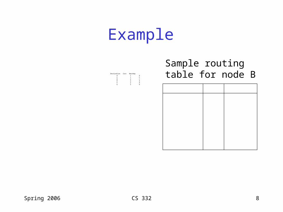
Spring 2006 CS 332 8

Example

Destination Cost NextHop A 1 A C 1 C D 2 C E 2 A F 2 A G 3 A

Sample routingtable for node B

Spring 2006 CS 332 9

Example of Update

• F detects that link to G has failed• F sets distance to G to infinity and sends update to A• A sets distance to G to infinity since it uses F to

reach G• A receives periodic update from C with 2-hop path

to G• A sets distance to G to 3 and sends update to F• F decides it can reach G in 4 hops via A

Spring 2006 CS 332 10

Note “distances” neednot be hop counts

Spring 2006 CS 332 11

Convergence Issues

• Distance vector schemes can converge slowly

A is downinitially, thencomes back up. Assume all routers update simultaneouslyvia common clock

Spring 2006 CS 332 12

Routing Loops

• Can happen because several nodes are updating routing tables concurrently

• Ex: The “count to infinity” problem

Initially all linesare up, then eitherA goes down or thelink between A andB is cut (same thingto B)

Numbers indicate estimated distanceto node A

Spring 2006 CS 332 13

Loop-Breaking Heuristics

• Set infinity to 16

• Split horizon– Don’t send routes learned from a given

neighbor back to that neighbor

• Split horizon with poison reverse– Reply to neighbor but give negative info

(such as infinite cost)

• These are Hacks!

Spring 2006 CS 332 14

Even Split Horizon Can Fail…

Spring 2006 CS 332 15

Even Split Horizon Can Fail…• Initially, A, B both have

distance 2 to D, C has distance 1 there.

• Line CD goes down

• C concludes that D is unreachable and reports this to A and B.

• A hears that B has a path of length 2 to D, so it assumes it can get to D in 3 hops. Similarly B assumes it can get to D in 3 hops.

• On next exchange they set distance to 4, etc.

Spring 2006 CS 332 16

Distance Vector Summary

• Good– Only need communicate with neighbors (so little

bandwidth is wasted on protocol overhead)

– Relatively little processing of info

• Bad– Count to infinity problem

– Slow convergence (the real issue)

• Despite this, RIP is popular– Because included in original BSD implementation

Spring 2006 CS 332 17

Link-State (OSPF)• Strategy

– send to all nodes (not just neighbors) information about directly connected links (not entire routing table)

• Link State Packet (LSP)– id of the node that created the LSP– cost of the link to each directly connected

neighbor– sequence number (SEQNO)– time-to-live (TTL) for this packet

Spring 2006 CS 332 18

Link-State (cont)

• Reliable flooding– store most recent LSP from each node– forward LSP to all nodes but one that sent it– generate new LSP periodically

• increment SEQNO– start SEQNO at 0 when reboot– decrement TTL of each stored LSP

• discard when TTL=0

Spring 2006 CS 332 19

Route Calculation• Dijkstra’s shortest path algorithm• Let

– N denotes set of nodes in the graph– l (i, j) denotes non-negative cost (weight) for edge (i, j)– s denotes this node– M denotes the set of nodes incorporated so far– C(n) denotes cost of the path from s to node n

M = {s}for each n in N - {s}

C(n) = l(s, n)while (N != M)

M = M union {w} such that C(w)is the minimum for all w in (N - M)for each n in (N - M)

C(n) = MIN(C(n), C (w) + l(w, n ))

If you don’t know Dijkstra’s algorithm,please see me!

Spring 2006 CS 332 20

Example

• Hi there

Spring 2006 CS 332 21

Link-State Summary

• Good– Converges relatively quickly

• Bad– Lots of information stored at each node because LSP

for each node in network must be stored at each node (scalability problem)

– Flooding of LSPs uses bandwidth

– Potential security issue (if false LSP propogates)

Spring 2006 CS 332 22

Open Shortest Path First (OSPF)

• Typical link-state but with enhancements– Authentication of routing messages

– Additional hierarchy (to help with scalability)

– Load balancing

Spring 2006 CS 332 23

Distance Vector vs Link-state

• Key philosophical difference– Distance vector talks only to directly connected

neighbors and tells them what is has learned

– Link-state talks to everybody, but only tells them what it knows

Spring 2006 CS 332 24

Metrics • Original ARPANET metric

– measures number of packets enqueued on each link– took neither latency or bandwidth into consideration

• New ARPANET metric– stamp each incoming packet with its arrival time (AT)– record departure time (DT)– when link-level ACK arrives, compute

Delay = (DT - AT) + Transmit + Latency

– if timeout, reset DT to departure time for retransmission – link cost = average delay over some time period

• Fine Tuning– compressed dynamic range– replaced dynamic with link utilization