Bumps in the Wire: NAT and DHCP Nick Feamster CS 4251 Computer Networking II Spring 2008.
Upload
richard-warrenCategory
view
226download
0
Intradomain Routing
CS 4251: Computer Networking IINick FeamsterSpring 2008

2
GeorgiaTech
Internet Routing Overview
• Today: Intradomain (i.e., “intra-AS”) routing• Wednesday: Interdomain routing
Comcast
Abilene
AT&T Cogent
Autonomous Systems (ASes)
3
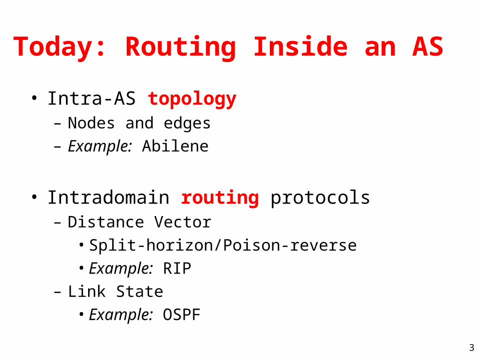
Today: Routing Inside an AS
• Intra-AS topology– Nodes and edges– Example: Abilene
• Intradomain routing protocols– Distance Vector
• Split-horizon/Poison-reverse• Example: RIP
– Link State• Example: OSPF

4
Topology Design
• Where to place “nodes”?– Typically in dense population centers
• Close to other providers (easier interconnection)• Close to other customers (cheaper backhaul)
– Note: A “node” may in fact be a group of routers, located in a single city. Called a “Point-of-Presence” (PoP)
• Where to place “edges”?– Often constrained by location of fiber

5
Node Clusters: Point-of-Presence (PoP)
• A “cluster” of routers in a single physical location
• Inter-PoP links– Long distances
– High bandwidth
• Intra-PoP links– Cables between racks or floors
– Aggregated bandwidth
PoP
6
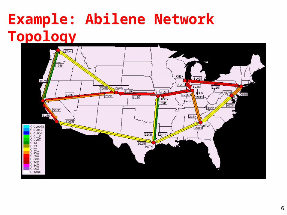
Example: Abilene Network Topology

7
Where’s Georgia Tech?
10GigE (10GbpS uplink)Southeast Exchange
(SOX) is at 56 Marietta Street

8
Another Example Backbone

9
Problem: Routing
• Routing: the process by which nodes discover where to forward traffic so that it reaches a certain node
• Within an AS: there are two “styles”– Distance vector: iterative, asynchronous, distributed– Link State: global information, centralized algorithm

10
Forwarding vs. Routing
• Forwarding: data plane– Directing a data packet to an outgoing link– Individual router using a forwarding table
• Routing: control plane– Computing paths the packets will follow– Routers talking amongst themselves– Individual router creating a forwarding table

11
Distance-Vector Routing
• Routers send routing table copies to neighbors• Routers compute costs to destination based on shortest
available path• Based on Bellman-Ford Algorithm
– dx(y) = minv{ c(x,v) + dv(y) }– Solution to this equation is x’s forwarding table
x y z
x 0 1 5
y
z
x y z
x
y 1 0 2
z
x y z
x
y
z 5 2 0
y
x z
1 2
5

12
Distance Vector Algorithm
Iterative, asynchronous: each local iteration caused by:
• Local link cost change
• Distance vector update message from neighbor
Distributed:• Each node notifies neighbors only
when its DV changes
• Neighbors then notify their neighbors if necessary
wait for (change in local link cost or message from neighbor)
recompute estimates
if DV to any destination has
changed, notify neighbors
Each node:

13
Good News Travels Quickly
• When costs decrease, network converges quickly
x y z
x 0 1 3
y 1 0 2
z 3 2 0
x y z
x 0 1 3
y 1 0 2
z 3 2 0
x y z
x 0 1 3
y 1 0 2
z 3 2 0
y
x z
1 2
5

14
Problem: Bad News Travels Slowly
y
x z
1 2
50
60
x y z
x 0 60 50
y 5 0 2
z 3 2 0
x y z
x 0 60 50
y 5 0 2
z 7 2 0
Note also that there is a forwarding loop between y and z.

15
It Gets Worse
• Question: How long does this continue?• Answer: Until z’s path cost to x via y is greater than 50.
y
x z
1 2
50
60
x y z
x 0 60 50
y 5 0 2
z 3 2 0
x y z
x 0 60 50
y 5 0 2
z 7 2 0

16
“Solution”: Poison Reverse
• If z routes through y to get to x, z advertises infinite cost for x to y
• Does poison reverse always work?
x y z
x 0 1 3
y 1 0 2
z 3 2 0
x y z
x 0 1 X
y 1 0 2
z X 2 0
x y z
x 0 1 3
y 1 0 2
z 3 2 0
y
x z
1 2
5

17
Does Poison Reverse Always Work?
y
x z
1 3
50
60
w
1
1
18
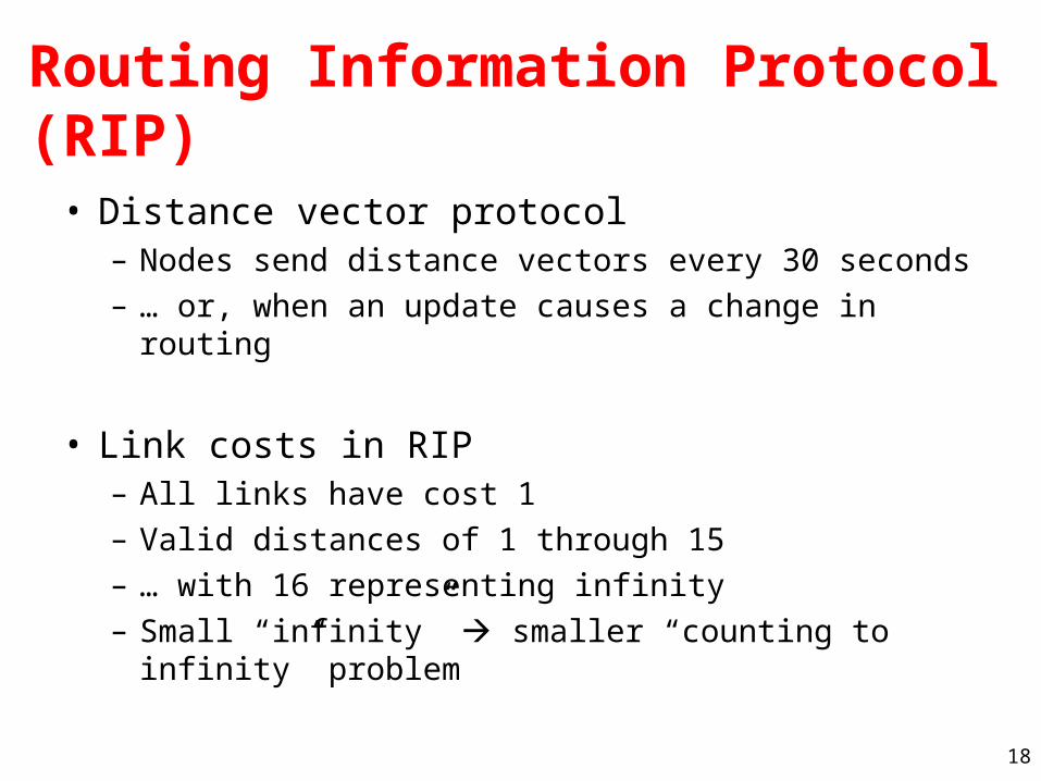
Routing Information Protocol (RIP)
• Distance vector protocol– Nodes send distance vectors every 30 seconds– … or, when an update causes a change in routing
• Link costs in RIP– All links have cost 1– Valid distances of 1 through 15– … with 16 representing infinity– Small “infinity” smaller “counting to infinity” problem

19
Link-State Routing• Keep track of the state of incident links
– Whether the link is up or down– The cost on the link
• Broadcast the link state– Every router has a complete view of the graph
• Compute Dijkstra’s algorithm• Examples:
– Open Shortest Path First (OSPF)– Intermediate System – Intermediate System (IS-IS)

20
Link-State Routing
• Idea: distribute a network map• Each node performs shortest path (SPF)
computation between itself and all other nodes• Initialization step
– Add costs of immediate neighbors, D(v), else infinite– Flood costs c(u,v) to neighbors, N
• For some D(w) that is not in N– D(v) = min( c(u,w) + D(w), D(v) )

21
Detecting Topology Changes• Beaconing
– Periodic “hello” messages in both directions– Detect a failure after a few missed “hellos”
• Performance trade-offs– Detection speed– Overhead on link bandwidth and CPU– Likelihood of false detection
“hello”

22
Broadcasting the Link State
• Flooding– Node sends link-state information out its links– The next node sends out all of its links except
the one where the information arrivedX A
C B D
(a)
X A
C B D
(b)
X A
C B D
(c)
X A
C B D
(d)

23
Broadcasting the Link State
• Reliable flooding– Ensure all nodes receive the latestlink-state
information
• Challenges– Packet loss– Out-of-order arrival
• Solutions– Acknowledgments and retransmissions– Sequence numbers– Time-to-live for each packet

24
When to Initiate Flooding
• Topology change– Link or node failure– Link or node recovery
• Configuration change– Link cost change
• Periodically– Refresh the link-state information– Typically (say) 30 minutes– Corrects for possible corruption of the data

25
Scaling Link-State Routing
• Message overhead– Suppose a link fails. How many LSAs will be flooded
to each router in the network?• Two routers send LSA to A adjacent routers• Each of A routers sends to A adjacent routers• …
– Suppose a router fails. How many LSAs will be generated?
• Each of A adjacent routers originates an LSA …

26
Scaling Link-State Routing• Two scaling problems
– Message overhead: Flooding link-state packets – Computation: Running Dijkstra’s shortest-path algorithm
• Introducing hierarchy through “areas”
Area 0areaborderrouter

27
Link-State vs. Distance-Vector• Convergence
– DV has count-to-infinity– DV often converges slowly (minutes) – DV has timing dependences– Link-state: O(n2) algorithm requires O(nE) messages
• Robustness– Route calculations a bit more robust under link-state– DV algorithms can advertise incorrect least-cost paths– In DV, errors can propagate (nodes use each others tables)
• Bandwidth Consumption for Messages– Messages flooded in link state

28
Open Shortest Paths First (OSPF)
• Key Feature: hierarchy• Network’s routers divided into areas• Backbone area is area 0• Area 0 routers perform SPF computation
– All inter-area traffic travles through Area 0 routers (“border routers”)
Area 0
29
Another Example: IS-IS• Originally: ISO Connectionless Network Protocol
– CLNP: ISO equivalent to IP for datagram delivery services– ISO 10589 or RFC 1142
• Later: Integrated or Dual IS-IS (RFC 1195)– IS-IS adapted for IP– Doesn’t use IP to carry routing messages
• OSPF more widely used in enterprise, IS-IS in large service providers

30
Area 49.001 Area 49.0002
Level-1Routing Level-2
Routing
Level-1Routing
Backbone
Hierarchical Routing in IS-IS
• Like OSPF, 2-level routing hierarchy – Within an area: level-1– Between areas: level-2– Level 1-2 Routers: Level-2 routers may also participate in L1 routing

31
ISIS on the Wire…

32
IS-IS Configuration on Abilene (atlang)
lo0 { unit 0 {
….family iso {
address 49.0000.0000.0000.0014.00; } …. }
isis { level 2 wide-metrics-only; /* OC192 to WASHng */ interface so-0/0/0.0 { level 2 metric 846; level 1 disable; }}
Only Level 2 IS-IS in Abilene
ISO Address Configured on Loopback Interface

33
IP Fast Reroute
• Interface protection (vs. path protection)– Detect interface/node failure locally– Reroute either to that node or one hop past
• Various mechanisms– Equal cost multipath– Loop-free Alternatives– Not-via Addresses

34
Equal Cost Multipath
• Set up link weights so that several paths have equal cost
• Protects only the paths for which such weights exist
Link not protected
S
D
I
15 5
55 5
15
15
5
20
35
ECMP: Strengths and Weaknesses
• Simple• No path stretch upon recovery
(at least not nominally)
• Won’t protect a large number of paths• Hard to protect a path from multiple failures• Might interfere with other objectives (e.g., TE)
Strengths
Weaknesses

36
Loop-Free Alternates
• Precompute alternate next-hop
• Choose alternate next-hop to avoid microloops:
S N
D
5
3 2 6
9
10
• More flexibility than ECMP• Tradeoff between loop-freedom and available
alternate paths
37
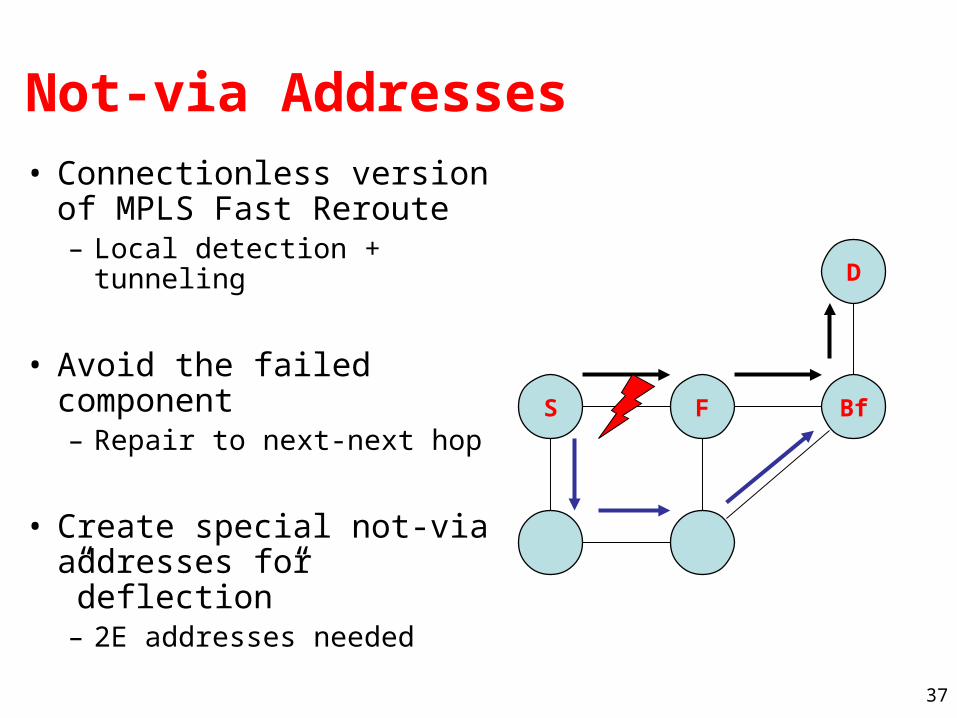
Not-via Addresses
• Connectionless version of MPLS Fast Reroute– Local detection + tunneling
• Avoid the failed component– Repair to next-next hop
• Create special not-via addresses for ”deflection”– 2E addresses needed
S F Bf
D
38
Not-via: Strengths and Weaknesses
• 100% coverage• Easy support for multicast traffic
– Due to repair to next-next hop
• Easy support for SRLGs
• Relies on tunneling– Heavy processing– MTU issues
• Suboptimal backup path lengths– Due to repair to next-next hop
Strengths
Weaknesses