Special course in Computer Science: Advanced Text...
43
Special course in Computer Science: Advanced Text Algorithms Lecture 2: Pattern Matching Algorithms Elena Czeizler and Ion Petre Department of IT, Abo Akademi Computational Biomodelling Laboratory http://users.abo.fi/pbostrom/kurser/textalgo/
Transcript of Special course in Computer Science: Advanced Text...

Special course in Computer Science: Advanced Text Algorithms
Lecture 2: Pattern Matching Algorithms
Elena Czeizler and Ion Petre Department of IT, Abo Akademi
Computational Biomodelling Laboratory http://users.abo.fi/pbostrom/kurser/textalgo/

Pattern Matching Problem
• The pattern matching problem is one of the most investigated problems in text algorithms.
• Implementations of algorithms for this problem are used daily for accessing information
• use Google search engine • make a data base query • use the “search” or “replace” commands in text editors
• Simple example of a pattern matching problem: • Find occurrences of the word “advanced” in the text “Special
course in Computer Science: advanced text algorithms”
2
3
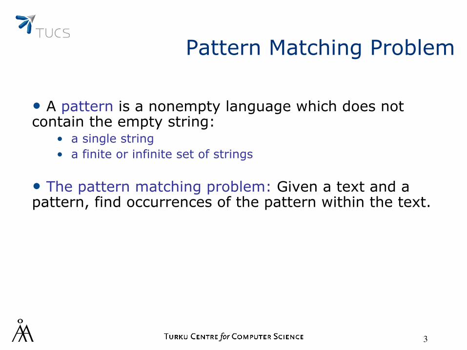
Pattern Matching Problem
• A pattern is a nonempty language which does not contain the empty string:
• a single string • a finite or infinite set of strings
• The pattern matching problem: Given a text and a pattern, find occurrences of the pattern within the text.
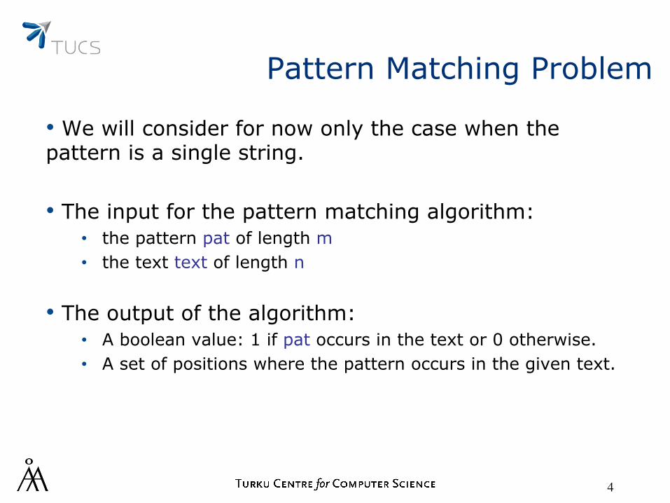
Pattern Matching Problem
• We will consider for now only the case when the pattern is a single string. • The input for the pattern matching algorithm:
• the pattern pat of length m • the text text of length n
• The output of the algorithm: • A boolean value: 1 if pat occurs in the text or 0 otherwise. • A set of positions where the pattern occurs in the given text.
4
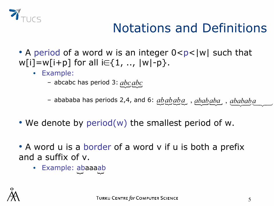
Notations and Definitions
• A period of a word w is an integer 0<p<|w| such that w[i]=w[i+p] for all i∈{1, .., |w|-p}.
• Example: – abcabc has period 3: – abababa has periods 2,4, and 6:
• We denote by period(w) the smallest period of w.
• A word u is a border of a word v if u is both a prefix and a suffix of v.
• Example: abaaaab
5
abcabc
abababa , abababa , ababab a

Notations and Definitions
• Just as in the case of periods, there are words which have several borders.
• Example: ababab
• Denote by Border(w) the longest nontrivial border of a word w, i.e., Border(w)≠w.
6
ababab
abababababab
ababab

Pattern Matching Algorithms
• We will discuss two fundamental pattern matching algorithms:
• Knuth-Morris-Pratt (KMP) algorithm • Boyer-Moore (BM) algorithm
• Both of them have two stages: • Pre-processing stage: computing some additional tables • Pattern-searching stage
7

Brute-force algorithm
• The scheme for a brute-force algorithm for the pattern-matching problem:
• This algorithm is the origin for both KMP and BM algorithms.
• The actual implementation of this algorithm depends on how we implement the function “check”, e.g., scanning the text from the left, or from the right, or other method.
8
for : 0 to do check if [ 1 .. ]i n m
pat text i i m= −
= + +

Brute-force algorithm
• Algorithm brute-force1 • the index i scans the positions of the text
• the index j scans the positions of the pattern
• if we found the pattern, then we stop
• otherwise, i.e., we have a mismatch between a character in the pattern and a character in the text, we increase i by 1 and we start comparing again pat and text.
9
: 0while do begin : 0; while and [ 1] [ 1] do : 1; if then return( ); : 1;end;return( )
ii n mj
j m pat j text i jj j
j m truei i
false
=
≤ −
=
< + = + +
= +
=
= +

Brute-force algorithm
• Algorithm brute-force1 Let text=aaaaabaa and pat=aaaba • i=0
aaab
aaaaabaa
• i=1 aaab
aaaaabaa
• i=2 aaaba
aaaaabaa
10
: 0while do begin : 0; while and [ 1] [ 1] do : 1; if then return( ); : 1;end;return( )
ii n mj
j m pat j text i jj j
j m truei i
false
=
≤ −
=
< + = + +
= +
=
= +
Brute-force algorithm
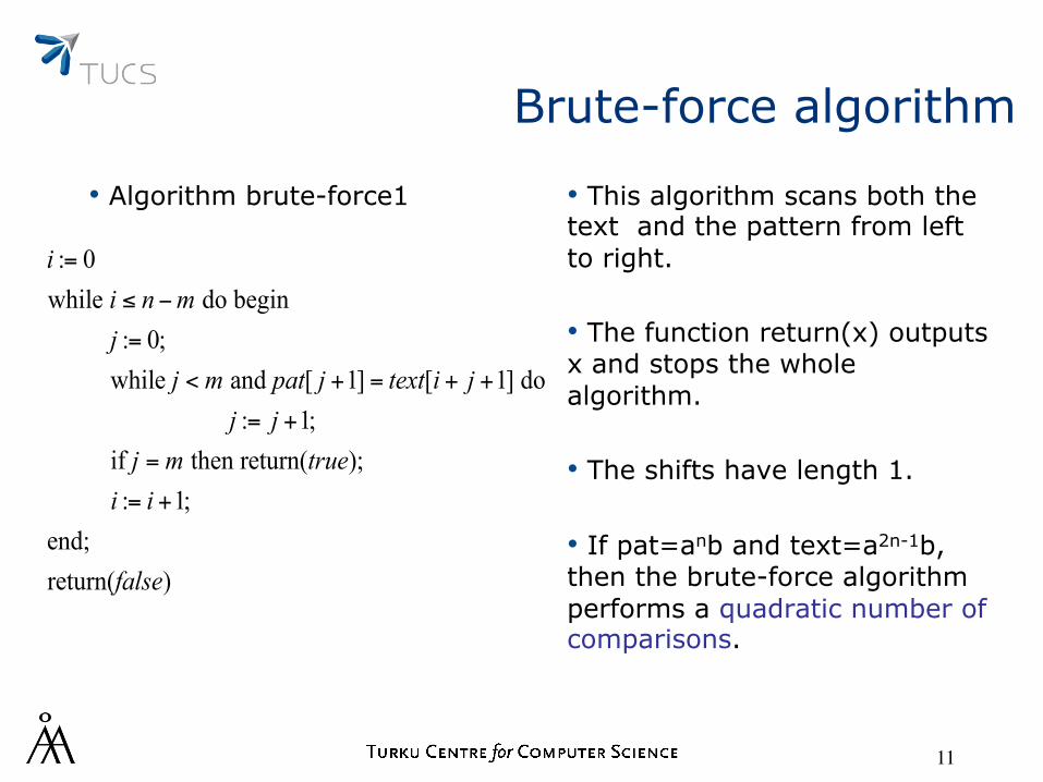
• Algorithm brute-force1 • This algorithm scans both the text and the pattern from left to right.
• The function return(x) outputs x and stops the whole algorithm.
• The shifts have length 1.
• If pat=anb and text=a2n-1b, then the brute-force algorithm performs a quadratic number of comparisons.
11
: 0while do begin : 0; while and [ 1] [ 1] do : 1; if then return( ); : 1;end;return( )
ii n mj
j m pat j text i jj j
j m truei i
false
=
≤ −
=
< + = + +
= +
=
= +
The Brute-force algorithm
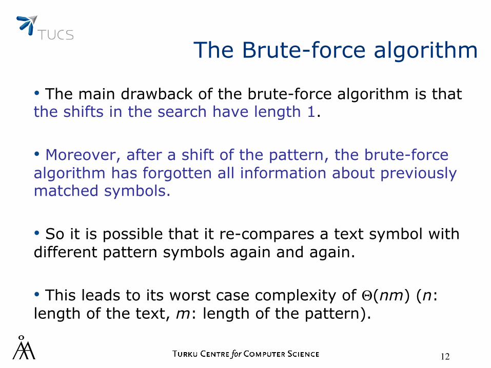
• The main drawback of the brute-force algorithm is that the shifts in the search have length 1.
• Moreover, after a shift of the pattern, the brute-force algorithm has forgotten all information about previously matched symbols.
• So it is possible that it re-compares a text symbol with different pattern symbols again and again.
• This leads to its worst case complexity of Θ(nm) (n: length of the text, m: length of the pattern).
12
The Brute-force algorithm
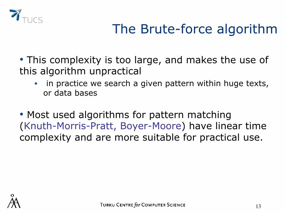
• This complexity is too large, and makes the use of this algorithm unpractical
• in practice we search a given pattern within huge texts, or data bases
• Most used algorithms for pattern matching (Knuth-Morris-Pratt, Boyer-Moore) have linear time complexity and are more suitable for practical use.
13

The Knuth-Morris-Pratt algorithm
• The Knuth-Morris-Pratt algorithm uses the information gained by previous symbol comparisons.
• It never compares again a text symbol that has already matched a pattern symbol.
• As a result, the complexity of the searching phase of the Knuth-Morris-Pratt algorithm is in O(n).
14

The Knuth-Morris-Pratt algorithm
• However, a pre-processing of the pattern is necessary in order to analyze its structure.
• The pre-processing phase has a complexity of O(m).
• Since m≤n, the overall complexity of the Knuth-Morris-Pratt algorithm is in O(n).
15

Morris-Pratt (MP) algorithm
• Let pat[1..j]=text[i+1..i+j] for some j≥1.
• We want to shift the search by more than 1 unit. • Safe shift s = a positive integer s such that there is no occurrence of the pattern at positions i, i+1, .., i+s-1, but there might be one at i+s.
16

Safe shift
• Suppose an occurrence of the pattern starts at position i+s and let k=j-s.
• Then pat[1..k] and pat[1..j] are suffixes of the same text: text[1..i+j]
• cond(j,k): pat[1..k] is a proper suffix of pat[1..j]
• So, s is a safe shift if k=j-s is the largest integer satisfying cond(j,k)
17

Safe shift
• cond(j,k): pat[1..k] is a proper suffix of pat[1..j]
• Denote Bord(j)= the largest integer k satisfying cond(j,k)
• Bord(j)=|Border(pat[1..j])|
• Then, the smallest safe shift is MP_Shift(j)=j-Bord(j)
18

Table of borders
• The table Bord, called the table of borders, is essential for this algorithm.
• It carries the information which allows us to compute the length of a safe shift (s=j-Bord(j)) in the case of a mismatch.
19

Example of a table of borders
• Bord(j)=|Border(pat[1..j])|
• Example: Let pat=abababababb. Then, Bord(1)=|Border(pat[1])|=|Border(a)|=0, Bord(2)=|Border(pat[1..2])|=|Border(ab)|=0, Bord(3)=|Border(pat[1..3])|=|Border(aba)|=1, Bord(4)=|Border(pat[1..4])|=|Border(abab)|=2,... Bord=[0,0,1,2,3,4,5,6,7,8,0]
• If j=0, pat[1..j]=ε, then the shift must be 1 and we define Bord(0)=-1
20
Computing the table of borders
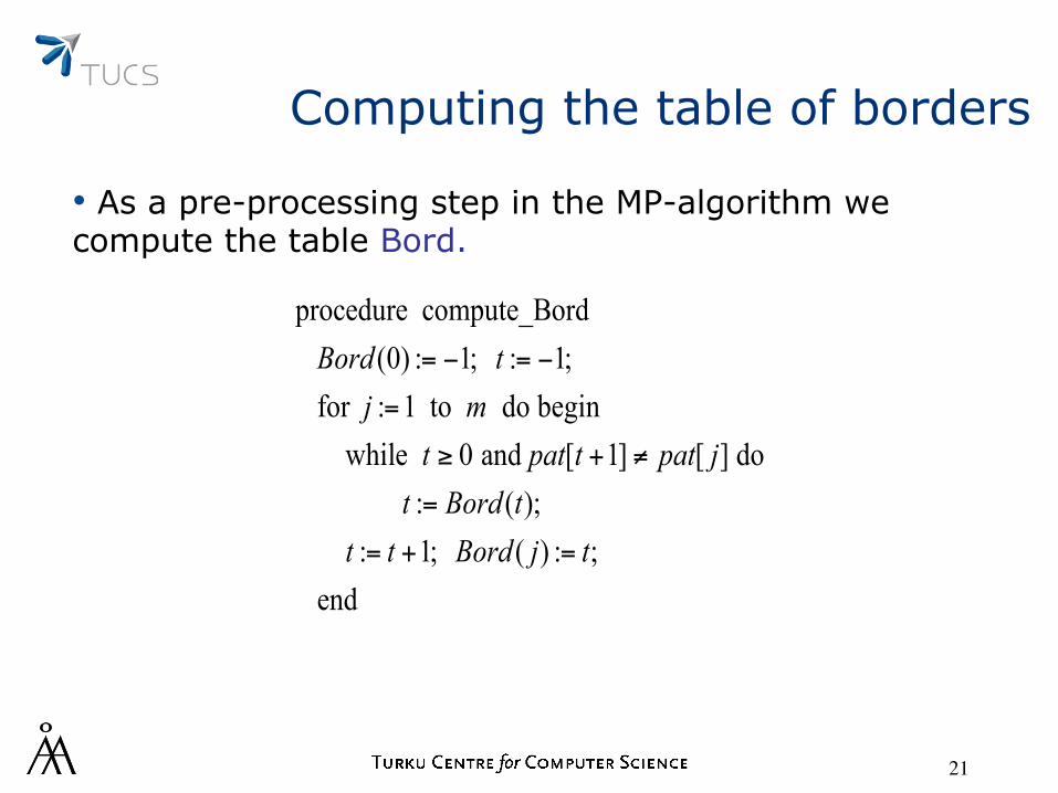
• As a pre-processing step in the MP-algorithm we compute the table Bord.
21
procedure compute_Bord (0) : 1; : 1; for : 1 to do begin while 0 and [ 1] [ ] do : ( ); : 1; ( ) : ; end
Bord tj m
t pat t pat jt Bord t
t t Bord j t
= − = −
=
≥ + ≠
=
= + =
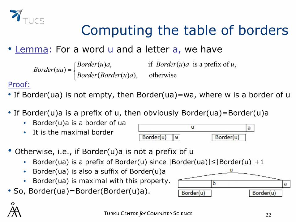
Computing the table of borders • Lemma: For a word u and a letter a, we have
Proof: • If Border(ua) is not empty, then Border(ua)=wa, where w is a border of u
• If Border(u)a is a prefix of u, then obviously Border(ua)=Border(u)a • Border(u)a is a border of ua • It is the maximal border
• Otherwise, i.e., if Border(u)a is not a prefix of u • Border(ua) is a prefix of Border(u) since |Border(ua)|≤|Border(u)|+1 • Border(ua) is also a suffix of Border(u)a • Border(ua) is maximal with this property.
• So, Border(ua)=Border(Border(u)a).
22
( ) , if ( ) is a prefix of ,( )
( ( ) ), otherwiseBorder u a Border u a u
Border uaBorder Border u a⎧
= ⎨⎩

Computing the table of borders • Lemma: The procedure compute_Bord applied to a string pat of length m produces the table of borders for pat. Proof: • The table Bord is computed sequentially by the procedure compute_Bord: from the prefix of length 1 to pat itself.
• At the beginning of each “for cycle” j, t=Bord(j-1), i.e., pat[1..t] is both a prefix and a suffix of pat[1..j-1], and is maximal with this property.
• If pat[t+1]=pat[j], i.e., the previous border can be extended by 1 character, i.e., Bord(j)=Bord(j-1)+1
• Otherwise, i.e., pat[t+1]≠pat[j], we compute recursively the new border in the while loop, according to the previous lemma.
23
procedure compute_Bord (0) : 1; : 1; for : 1 to do begin while 0 and [ 1] [ ] do : ( ); : 1; ( ) : ; end
Bord tj m
t pat t pat jt Bord t
t t Bord j t
= − = −
=
≥ + ≠
=
= + =
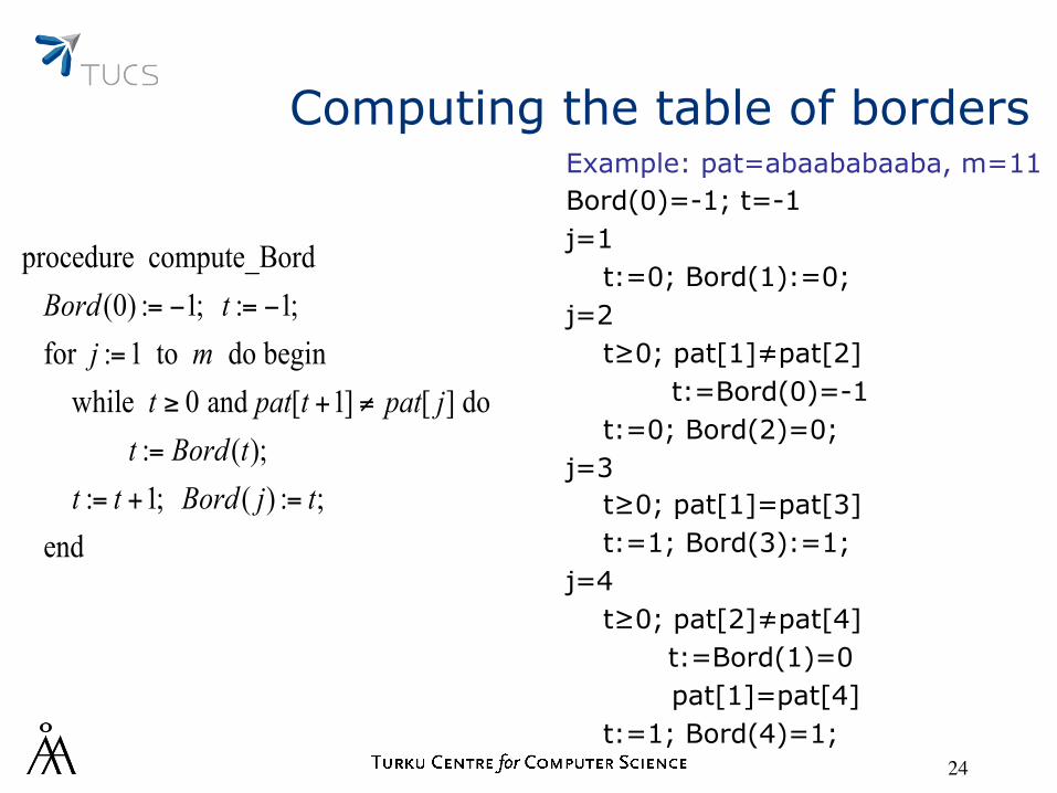
Computing the table of borders Example: pat=abaababaaba, m=11 Bord(0)=-1; t=-1 j=1 t:=0; Bord(1):=0; j=2 t≥0; pat[1]≠pat[2]
t:=Bord(0)=-1 t:=0; Bord(2)=0; j=3 t≥0; pat[1]=pat[3] t:=1; Bord(3):=1; j=4 t≥0; pat[2]≠pat[4] t:=Bord(1)=0
pat[1]=pat[4] t:=1; Bord(4)=1;
24
procedure compute_Bord (0) : 1; : 1; for : 1 to do begin while 0 and [ 1] [ ] do : ( ); : 1; ( ) : ; end
Bord tj m
t pat t pat jt Bord t
t t Bord j t
= − = −
=
≥ + ≠
=
= + =
Computing the table of borders
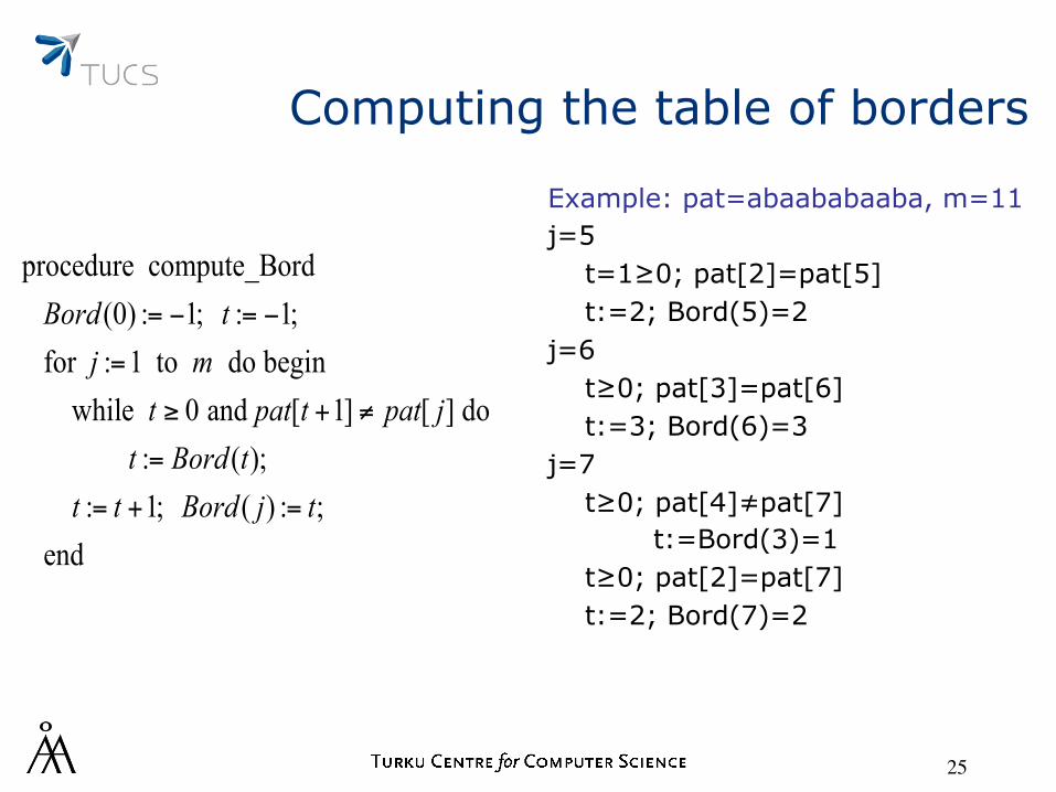
Example: pat=abaababaaba, m=11 j=5 t=1≥0; pat[2]=pat[5] t:=2; Bord(5)=2 j=6 t≥0; pat[3]=pat[6] t:=3; Bord(6)=3 j=7 t≥0; pat[4]≠pat[7]
t:=Bord(3)=1 t≥0; pat[2]=pat[7] t:=2; Bord(7)=2
25
procedure compute_Bord (0) : 1; : 1; for : 1 to do begin while 0 and [ 1] [ ] do : ( ); : 1; ( ) : ; end
Bord tj m
t pat t pat jt Bord t
t t Bord j t
= − = −
=
≥ + ≠
=
= + =
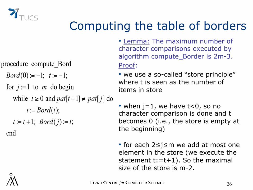
Computing the table of borders • Lemma: The maximum number of character comparisons executed by algorithm compute_Border is 2m-3. Proof: • we use a so-called “store principle” where t is seen as the number of items in store
• when j=1, we have t<0, so no character comparison is done and t becomes 0 (i.e., the store is empty at the beginning)
• for each 2≤j≤m we add at most one element in the store (we execute the statement t:=t+1). So the maximal size of the store is m-2.
26
procedure compute_Bord (0) : 1; : 1; for : 1 to do begin while 0 and [ 1] [ ] do : ( ); : 1; ( ) : ; end
Bord tj m
t pat t pat jt Bord t
t t Bord j t
= − = −
=
≥ + ≠
=
= + =

Computing the table of borders • each time we execute statement t:=Bord(t), t is decreased, i.e., we eliminate some elements from the store.
• So there are at most m-2 unsuccessful character comparisons pat[t+1]≠pat[j] (for each of them we execute the statemet t:=Bord(t))
• For each 2≤j≤m, there is at most one successful character comparison.
• Thus the total number of character comparisons is at most (m-2)+(m-1)=2m-3
27
procedure compute_Bord (0) : 1; : 1; for : 1 to do begin while 0 and [ 1] [ ] do : ( ); : 1; ( ) : ; end
Bord tj m
t pat t pat jt Bord t
t t Bord j t
= − = −
=
≥ + ≠
=
= + =
Morris-Pratt (MP) algorithm
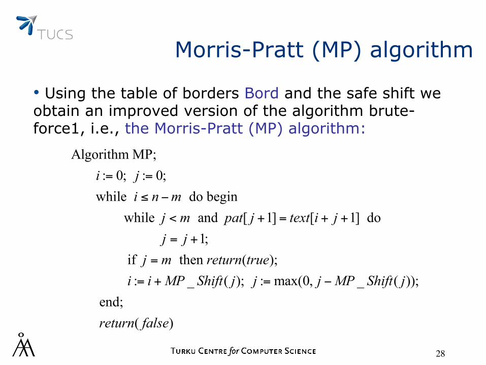
• Using the table of borders Bord and the safe shift we obtain an improved version of the algorithm brute-force1, i.e., the Morris-Pratt (MP) algorithm:
28
Algorithm MP; : 0; : 0; while do begin while and [ 1] [ 1] do 1; if then ( );
i ji n m
j m pat j text i jj j
j m return true
= =
≤ −
< + = + +
= +
=
: _ ( ); : max(0, _ ( )); end; ( )
i i MP Shift j j j MP Shift j
return false
= + = −

Morris-Pratt (MP) algorithm
29

Morris-Pratt (MP) algorithm
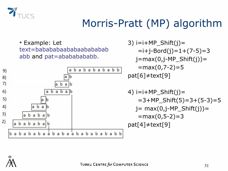
• Example: Let text=babababaababaabababababb and pat=abababababb.
1) i=0, j=0 pat[1]≠text[1]
2) i=i+MP_Shift(j)= =i+j-Bord(j)=0+0-(-1)=1; j=max(0,j-MP_Shift(j))=0
pat[1]=text[2]; pat[2]=text[3] pat[3]=text[4]; pat[4]=text[5] pat[5]=text[6]; pat[6]=text[7] pat[7]=text[8]; pat[8]≠text[9] j=7, i=1
30
Morris-Pratt (MP) algorithm
3) i=i+MP_Shift(j)= =i+j-Bord(j)=1+(7-5)=3 j=max(0,j-MP_Shift(j))= =max(0,7-2)=5 pat[6]≠text[9] 4) i=i+MP_Shift(j)= =3+MP_Shift(5)=3+(5-3)=5 j= max(0,j-MP_Shift(j))= =max(0,5-2)=3 pat[4]≠text[9]
31
• Example: Let text=babababaababaabababababb and pat=abababababb.

Morris-Pratt (MP) algorithm • Lemma: The time complexity of the algorithm MP is linear in the length of the text (i.e., O(n)). The maximal number of character comparisons is 2n-m. Proof: • Let T(n) be the maximal number of comparisons pat[j+1]=text[i+j+1].
• There are at most n-m+1 unsuccessful comparisons: at most one for each i (0 ≤ i ≤ n-m)
• 0≤i+j≤n
32
Algorithm MP; : 0; : 0; while do begin while and [ 1] [ 1] do 1; if then ( ); : _ ( );
i ji n mj m
pat j text i jj j
j m return truei i MP Shift j
= =
≤ −
<
+ = + +
= +
=
= +
: max(0, _ ( )); end; ( )
j j MP Shift j
return false
= −

Morris-Pratt (MP) algorithm • Each time we have a successful comparison we increase i+j by 1 and this value never decreases.
• So there are at most n successful comparisons.
• If the first comparison is unsuccessful, then we do not have any successful comparison for i=0.
• So, T(n)≤n+n-m=2n-m.
• If text=an and pat=ab, then we actually have T(n)=2n-m
33
Algorithm MP; i := 0; j := 0; while i ≤ n−m do begin while j <m and pat[ j +1]= text[i + j +1] do j = j +1; if j =m then return(true); i := i +MP _ Shift( j); j := max(0, j −MP _ Shift( j)); end; return( false)

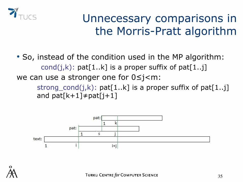
Unnecessary comparisons in the Morris-Pratt algorithm
• If we had a mismatch in the MP-algorithm , i.e., pat[j+1]≠text[i+j+1], then the next comparison is between text[i+j+1] and pat[k+1], where k=Bord(j).
• If pat[k+1]=pat[j+1], then we have the same mismatch.
34
Unnecessary comparisons in the Morris-Pratt algorithm
• So, instead of the condition used in the MP algorithm: cond(j,k): pat[1..k] is a proper suffix of pat[1..j]
we can use a stronger one for 0≤j<m: strong_cond(j,k): pat[1..k] is a proper suffix of pat[1..j] and pat[k+1]≠pat[j+1]
35
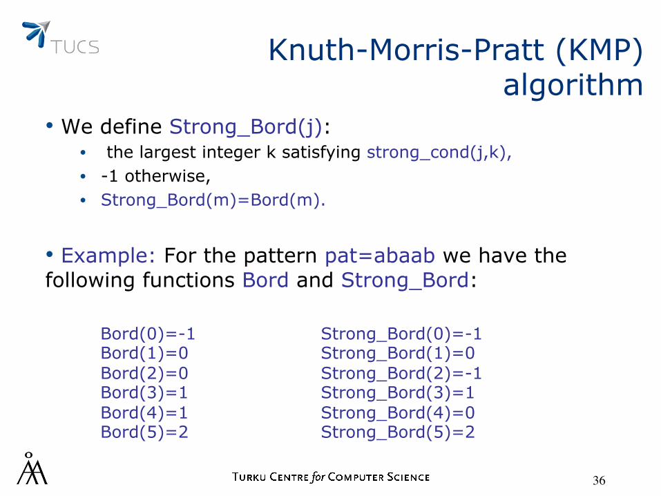
Knuth-Morris-Pratt (KMP) algorithm
• We define Strong_Bord(j): • the largest integer k satisfying strong_cond(j,k), • -1 otherwise, • Strong_Bord(m)=Bord(m).
• Example: For the pattern pat=abaab we have the following functions Bord and Strong_Bord:
36
Bord(0)=-1 Bord(1)=0 Bord(2)=0 Bord(3)=1 Bord(4)=1 Bord(5)=2
Strong_Bord(0)=-1 Strong_Bord(1)=0 Strong_Bord(2)=-1 Strong_Bord(3)=1 Strong_Bord(4)=0 Strong_Bord(5)=2
Knuth-Morris-Pratt (KMP) algorithm
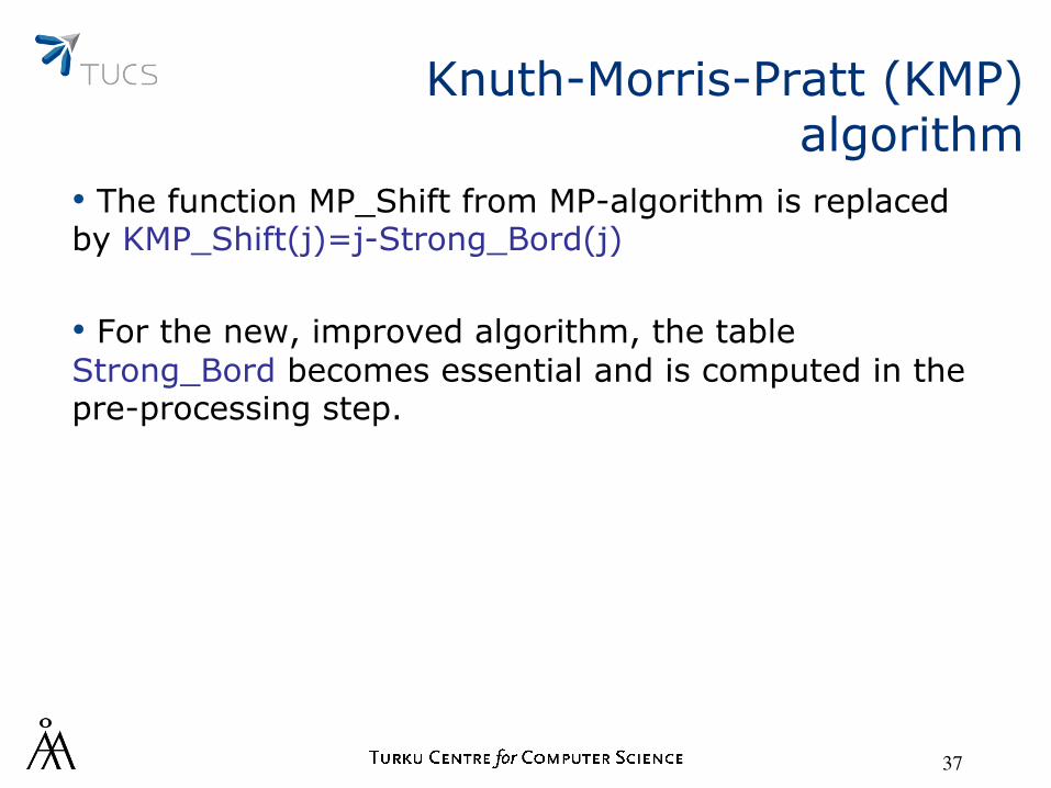
• The function MP_Shift from MP-algorithm is replaced by KMP_Shift(j)=j-Strong_Bord(j)
• For the new, improved algorithm, the table Strong_Bord becomes essential and is computed in the pre-processing step.
37

Computation of the table Strong_Bord
• Let t=Bord(j)
• If pat[t+1]≠pat[j+1], then Strong_Bord(j)=Bord(j).
• Otherwise, i.e., pat[t+1]=pat[j+1], we have Strong_Bord(j)=Strong_Bord(t) (=Strong_Bord(Bord(j)))
• Strong_Bord(|pat|)=Bord(|pat|) (as if pat is followed by an end marker)
38

Computation of the table Strong_Bord
39
• Example: For the pattern pat=abam-2, the table Strong_Bord computed by this algorithm is: Strong_Bord(0)=-1, Strong_Bord(1)=0, Strong_Bord(2)=-1, Strong_Bord(j)=1, for all 3≤j≤m.
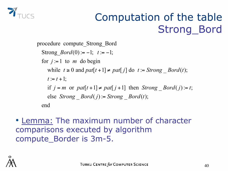
procedure compute_Strong_Bord Strong_ (0) : 1; : 1; for : 1 to do begin while 0 and [ 1] [ ] do : _ ( ); : 1; if or [ 1] [ 1]
Bord tj m
t pat t pat j t Strong Bord tt tj m pat t pat j
= − = −
=
≥ + ≠ =
= +
= + ≠ + then _ ( ) : ; else _ ( ) : _ ( ); end
Strong Bord j tStrong Bord j Strong Bord t
=
=
Computation of the table Strong_Bord
• Lemma: The maximum number of character comparisons executed by algorithm compute_Border is 3m-5.
40
procedure compute_Strong_Bord Strong_ (0) : 1; : 1; for : 1 to do begin while 0 and [ 1] [ ] do : _ ( ); : 1; if or [ 1] [ 1]
Bord tj m
t pat t pat j t Strong Bord tt tj m pat t pat j
= − = −
=
≥ + ≠ =
= +
= + ≠ + then _ ( ) : ; else _ ( ) : _ ( ); end
Strong Bord j tStrong Bord j Strong Bord t
=
=
Knuth-Morris-Pratt (KMP) algorithm
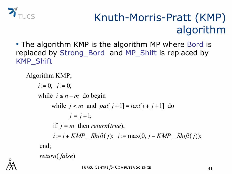
• The algorithm KMP is the algorithm MP where Bord is replaced by Strong_Bord and MP_Shift is replaced by KMP_Shift
41
Algorithm KMP; : 0; : 0; while do begin while and [ 1] [ 1] do 1; if then ( );
i ji n m
j m pat j text i jj j
j m return true
= =
≤ −
< + = + +
= +
=
: _ ( ); : max(0, _ ( )); end; ( )
i i KMP Shift j j j KMP Shift j
return false
= + = −

Knuth-Morris-Pratt (KMP) algorithm
• Lemma: The complexity of Knuth-Morris-Pratt algorithm is in O(n).
• The complexity of the searching phase of the Knuth-Morris-Pratt algorithm is in O(n).
• The pre-processing phase has a complexity of O(m).
• Since m≤n, the overall complexity of the Knuth-Morris-Pratt algorithm is in O(n).
42

Literature
• The slides follow the presentation in • Maxime Crochemore, Wojciech Rytter, Jewels of stringology,
World Scientific, 2002.
• The book by Gusfield presents the algorithm in a quite different way
43