Spatial Linkages, Global Shocks, and Local Labor Markets ...ka265/research/LaborSupplyTrade/Adao...

Spatial Linkages, Global Shocks, and Local Labor

Markets: Theory and Evidence∗

Rodrigo Adao

Chicago Booth

Costas Arkolakis

Yale

Federico Esposito

Tufts

February 2019

Abstract

How do shocks to economic fundamentals in the world economy affect local labor

markets? In a framework with a flexible structure of spatial linkages, we characterize the

model-consistent shock exposure of a local market as the exogenous shift in its production

revenues and consumption costs. In general equilibrium, labor outcomes in any market

respond directly to the market’s own shock exposure, and indirectly to other markets

shocks exposures. We show how spatial linkages control the size and the heterogeneity

of these indirect effects. We then develop a new estimation methodology – the Model-

implied Optimal IV (MOIV) – that exploits quasi-experimental variation in economic

shocks to estimate spatial linkages and evaluate their counterfactual implications.

Applying our methodology to US Commuting Zones, we find that difference-in-difference

designs based on model-consistent measures of local shock exposure approximate well

the differential effect of international trade shocks across CZs, but miss around half of

the aggregate effect, partly due to the offsetting action of indirect effects.

∗We thank Pol Antras, Marta Bengoa, Martin Beraja, Varadarajan V. Chari, Lorenzo Caliendo, ArnaudCostinot, Javier Cravino, Jonathan Dingel, Dave Donaldson, Max Dvorkin, Farid Farrokhi, Gordon Hanson,Rich Hornbeck, Erik Hurst, Samuel Kortum, Andrew McCallum, Eduardo Morales, Elias Papaioannou, AmilPetrin, Steve Redding, Esteban Rossi-Hansberg, Daniel Trefler, Jonathan Vogel, David Weinstein, as well asnumerous participants at many seminars and conferences for helpful suggestions and comments. We alsothank Zijian He, Guangbin Hong, Jack Liang, and Josh Morris-Levenson for excellent research assistance.All errors are our own.

1 Introduction

How large and heterogeneous are the gains and losses in a country following an aggregate

economic shock, such as a change in trade policy or a productivity boom in a foreign country?

The lack of exogenous variation in such aggregate shocks makes it challenging to answer

these questions in general equilibrium (see Nakamura and Steinsson (2018)). To circumvent

this identification problem, economists have followed two different approaches. On the one

hand, there is a growing literature that exploits quasi-experimental variation in cross-regional

exposure to aggregate economic shocks to credibly estimate their differential impact on

regional economic outcomes.1 However, extrapolating counterfactual predictions in general

equilibrium from the estimated differential responses is not straightforward (Kline and Moretti,

2014; Beraja, Hurst, and Ospina, 2016; Muendler, 2017), a problem particularly acute in the

presence of spatial links that generate endogenous correlation in regional outcomes (Moretti,

2011). On the other hand, a growing literature relies on general equilibrium quantitative

analysis that enables the computation of the aggregate effect of counterfactual changes in

trade costs and productivity.2 This literature has not clearly evaluated how the aggregate

counterfactual predictions are connected to the evidence on differential regional responses to

exogenous shocks and how robust they are to specifications of the model’s general equilibrium

forces.

Our paper provides a bridge between these two approaches by formalizing a methodology

that exploits quasi-experimental variation to credibly estimate cross-regional differential

responses to various economics shocks, and simultaneously enables to robustly aggregate the

counterfactual implications of these estimates in general equilibrium. We start by providing

a theoretical characterization of how spatial links determine the impact of changes in trade

costs and productivity in the world economy on local labor markets that is robust within a

class of general equilibrium spatial models. Using this characterization, we derive measures

of the local exposure to economic shocks that are directly connected to the reduced-form

predictions of the model. We establish that the aggregation problem is equivalent to the

measurement of the indirect effect of a market’s shock exposure on other markets, which

themselves depend on the strength of spatial links in the economy. We then propose a

1There is a vast literature studying the differential effect of international trade shocks across regionaleconomies – e.g., see Topalova (2010), Kovak (2013), Autor, Dorn, and Hanson (2013), Acemoglu et al.(2016), Dix-Carneiro and Kovak (2017), Pierce and Schott (2016b). Several papers have also documented asignificant effect of local exposure to technological shocks on regional labor market outcomes – e.g., see Autorand Dorn (2013), Bustos, Caprettini, and Ponticelli (2016), and Acemoglu and Restrepo (2017). Finally, anemerging literature evaluates the effect of regional exposure to macroeconomic shocks on regional outcomes –e.g., see Mian and Sufi (2014), Nakamura and Steinsson (2014) and Beraja, Hurst, and Ospina (2016).

2For reviews of these quantitative frameworks, see Costinot and Rodriguez-Clare (2013) for gravity trademodels and Redding and Rossi-Hansberg (2016) for spatial models.

1

methodology to estimate spatial links that combines quasi-experimental variation in economic

shocks and our model-consistent exposure measures. In our empirical application to US

Commuting Zones, we quantify the importance of such spatial links in shaping the general

equilibrium responses to the recent China’s productivity boom.

The first part of the paper examines the role of spatial linkages in shaping the impact of

economic shocks on labor markets outcomes across regions. The starting point of our analysis

is a multi-region economy with a single freely-traded homogeneous good. We introduce two

functions that govern spatial links in terms of endogenous labor supply and labor productivity.

The combination of these two functions into a single ‘‘labor module’’ controls the magnitude

of the reduced-form response of regional employment and wages to productivity shocks in the

own local market – the direct shock effect – and in other local markets in the economy – the

indirect shock effects. Thus, these indirect general equilibrium effects are part of the total

impact of the economic shock on any region, affecting both the differential and the aggregate

responses of regional outcomes.

We provide three results to clarify this point using a first-order approximation of the

model’s general equilibrium predictions. We first show that, if spatial links are not present

(i.e., markets are segmented), the differential response of local outcomes to changes in local

productivity yields both the differential and the aggregate effects of productivity shocks in

general equilibrium. These effects are increasing in the combined magnitude of the own-market

elasticity of labor supply and labor productivity. Second, adding spatial linkages that are

homogeneous across markets implies a reduced-form response that entails an ‘‘endogenous’’

time fixed-effect, containing the sum of the symmetric indirect spillovers of productivity

shocks in all regions. Conditional on the spatial distribution of the shock, the magnitude

of the fixed-effect is increasing in the combined strength of the symmetric spatial links in

the economy. Finally, if linkages are heterogeneous across markets, then indirect spillovers

are also heterogeneous and, therefore, are not absorbed by a fixed-effect. However, weak

conditions guaranteeing the uniqueness of the spatial equilibrium imply that indirect effects

are bounded by the magnitude of the spatial links in the ‘‘labor module.’’

We then extend our analysis to a Generalized Spatial Economy that features differentiated

goods produced by multiple local labor markets, i.e. sector-region pairs. This specification

gives rise to an additional source of spatial links that takes the form of a bilateral trade

demand function. These trade links also generate indirect effects across markets, which are

absent only in the special case of an economic shock to a set of markets effectively forming

a small open economy. By properly specifying the shape of spatial links, we show that our

model is general enough to replicate the labor market predictions of a wide class of trade

and geography models. Accordingly, our results are robust to the particular assumptions of

2

various models regulating the strength of connections among local labor markets in general

equilibrium.3

We use this environment to propose a generalized way to measure exposure of local

markets to economic shocks in the world economy. This connects the first part of our paper,

the theoretical characterization, to the second part, the measurement and estimation. In our

general equilibrium model, we characterize the direct and indirect effects on local outcomes

created by two model-consistent measures of shock exposure of different markets. These

measures capture the shock to both sides of a market’s terms-of-trade: the shift in (i) the

world demand for local labor, which we name ‘‘revenue exposure,’’ and (ii) the local cost of

world products, which we name ‘‘consumption exposure.’’ The theory illustrates that these

two exposure measures have opposite effects on local employment. In the special case of

gravity trade links, they are effectively the partial equilibrium impact of the shock on the

measures of firm and consumer market access introduced by Redding and Venables (2004).

These exposure measures allow the empirical evaluation of the impact of exogenous economic

shocks on local labor markets in a model-consistent way. In fact, the indirect effect of these

measures build the link between estimated differential effects of local shock exposure and the

model’s counterfactual predictions in general equilibrium. This is in contrast with quantitative

exercises that have enough degrees of freedom to match entirely the cross-regional data, but

do not evaluate the causal implications of the model following exogenous economics shocks.

In light of these results, the second part of the paper develops a methodology to estimate

spatial links within a country. First, we outline a data generating process in which markets

experience changes in productivity and amenities, and spatial links depend on an unknown

vector of ‘‘deep’’ structural parameters. Conditional on this vector, we establish conditions

for the recovery of unobservable shocks in each market’s productivity and amenities using

observed changes in labor outcomes across markets.4 Second, given these structural residuals,

the parameter vector can be estimated using a class of moment conditions that combine

the recovered local shocks and arbitrary functions of exogenous foreign cost shocks. This

step exploits quasi-experimental variation in shock exposure across markets, as in Topalova

(2010), Kovak (2013) and Autor, Dorn, and Hanson (2013). Finally, we follow the Optimal IV

3These frameworks include: (i) Neoclassical trade theories with external economies of scale (as in Ethier(1982a,b)) and without (as in Anderson (1979) and Eaton and Kortum (2002)); (ii) New trade theory modelswith homogeneous firms (as in Krugman (1980)); (iii) New economic geography models (as in Krugman (1991)and Allen and Arkolakis (2014)); (iv) Roy spatial assignment models (as in Galle, Rodriguez-Clare, and Yi(2017) and Adao (2015)). Finally, the model specified without trade frictions yields predictions equivalent tothe framework in Rosen (1979)-Roback (1982) and, more recently, in Kline and Moretti (2014).

4This step is distinct from other works in spatial economics, that invert structural residuals using theentire general equilibrium structure of the model, as in Allen and Arkolakis (2014), Monte, Redding, andRossi-Hansberg (2018), and Faber and Gaubert (2016).

3

approach of Chamberlain (1987) to characterize the ‘‘optimal’’ variance-minimizing estimator

within this class and its Two-Step GMM feasible implementation. In particular, we show

that such an estimator uses the impact of observed cost shocks on the endogenous variables

predicted by our general equilibrium model – the Model-implied Optimal IV (MOIV).5

Intuitively, our methodology is a generalization of shift-share instrumental variables applied

in many empirical papers since Bartik (1991) and Altonji and Card (1991). Rather than using

an ad-hoc local exposure ‘‘share’’ to the aggregate ‘‘shift,’’ the MOIV relies on the general

equilibrium model to dictate the heterogeneity in the impact of the ‘‘shift’’ on different local

labor markets.

The last part of the paper applies our methodology to quantify the importance of spatial

links for the impact of international trade shocks on employment across Commuting Zones

(CZs) in the United States. Specifically, we parametrize the Generalized Spatial Economy by

using a multiple-industry gravity trade structure with parameters controlling links in labor

supply and productivity across sectors and regions. Our empirical application entails 722 CZs

in the US, 58 foreign countries, 31 manufacturing industries, one non-manufacturing sector,

and non-employment through a home sector. In the estimation of the model’s structural

parameters, we exploit quasi-experimental variation induced by industry-level Chinese export

growth between 1997 and 2007, as in Autor, Dorn, and Hanson (2013). To evaluate the

robustness of our results, we also report estimates based on alternative measures of China’s

competitiveness shock used in the literature – e.g., the removal of tariff uncertainty on

Chinese imports (Pierce and Schott, 2016a), and changes in Chinese firms productivity (Hsieh

and Ossa, 2016).

The implementation of our empirical methodology yields estimates of the structural

parameters governing cross-market links in our model. Specifically, we estimate an elasticity of

employment to real wage of 0.1 in the manufacturing sector and 0.3 in the non-manufacturing

sector. Our estimates also suggest that the between-region elasticity of labor supply is

one-third of the between-sector elasticity. Moreover, using a specification similar to the one

proposed in Ahlfeldt et al. (2015), we estimate a local agglomeration force with a similar

magnitude as that in a Krugman model, as well as productivity spillovers that decline with

distance. To assess our model’s counterfactual implications, we compare the cross-regional

patterns of actual changes in manufacturing employment with those predicted by our model

5The approach of Chamberlain (1987) has been used in partial equilibrium models by Berry, Levinsohn,and Pakes (1999), Petrin (2002), and Reynaert and Verboven (2014). In general equilibrium, model-impliedinstruments have been also used recently in Monte, Redding, and Rossi-Hansberg (2018), Faber and Gaubert(2016), Eckert and Peters (2018), and Allen and Donaldson (2018). Our work is most close to the approachof Allen, Arkolakis, and Takahashi (2018) in a gravity setup. Our contribution is, for a general class ofspatial models, to formally establish a class of consistent estimators and among them characterize the optimalestimator, effectively an aggregation function over an exogenous shock.

4

in response to the Chinese competition shock. We find a positive and statistically significant

relationship that holds even conditional on the CZ’s initial labor market and demographic

conditions.

Finally, we decompose the model’s predicted changes in labor outcomes in each CZ into

the direct and the indirect general equilibrium effects of the shock exposure of all CZs. We

obtain three main results. First, stronger import competition from China reduces the world

demand for labor in the manufacturing sector for the majority of CZs. Cross-regional variation

in the manufacturing ‘‘revenue exposure’’ is a strong predictor of the cross-regional variation

in manufacturing employment and wage losses in our general equilibrium model. Second, the

positive impact of lower consumption costs is fairly homogeneous across CZs and compensates

half of the average negative impact of higher foreign import competition. Third, our estimates

of the spatial links in the US yield compensating indirect effects from other CZs, which

further offset the negative impact on the local manufacturing sector. Interestingly, these

general equilibrium indirect effects do not substantially affect the cross-regional variation due

to the direct exposure, but shift the employment responses up by a magnitude equivalent to

half of the average negative impact of the shock to manufacturing revenues.

The use of quasi-experimental variation in regional shock exposure has become a powerful

tool in the investigation of the labor market consequences of a variety of economic shocks

since the seminal papers by Altonji and Card (1991), Bartik (1991) and Blanchard and Katz

(1992). More recently, empirical specifications point towards strong differential cross-regional

and cross-sectoral effects of exposure to international shocks on employment and wages

(e.g., Topalova (2010), Kovak (2013), Autor, Dorn, and Hanson (2013), Autor et al. (2014),

Pierce and Schott (2016a)). We contribute to this literature by establishing theoretically

and empirically the role of spatial links in generating indirect spillover effects of local shock

exposure on other markets. In a sense, as in Heckman, Lance, and Taber (1998), we

characterize the effect of ‘‘treated’’ markets on ‘‘non-treated’’ markets that is part of the

response of local outcomes in general equilibrium. In addition, we show that trade links affect

the measurement of the exposure of any particular market to an economic shock in the world

economy – that is, a market’s ‘‘treatment’’ intensity in terms of production revenues and

consumption costs.6

Our paper is also related to a growing literature that relies on general equilibrium

quantitative analysis to compute the aggregate effect of counterfactual changes in trade costs

6Heterogeneity in spatial links also gives rise to heterogeneity in the direct effect of the own market’sshock exposure – i.e., heterogeneous treatment effects across regions. This heterogeneity has been emphasizedrecently by Monte, Redding, and Rossi-Hansberg (2018) in a model with commuting flows across regions.Instead, we focus on the implication of spatial links for the measurement of shock exposure and the magnitudeof indirect effects.

5

and productivity, as in Allen and Arkolakis (2014) and Caliendo et al. (2018b). Recently,

several papers have focused on quantifying the labor market consequences of the integration

of China into the world economy (e.g., Galle, Rodriguez-Clare, and Yi (2017), Lee (2015),

Hsieh and Ossa (2016), and Caliendo, Dvorkin, and Parro (2018a)). Our theoretical results

establish that the reduced-form predictions of this class of quantitative models depend on

three functions governing spatial links, which can be estimated from the impact of economic

shocks on trade and labor outcomes across local markets. Given estimates of these functions,

the model’s predictions are robust to any specific micro-foundations. In this sense, our analysis

characterizes ‘‘deep’’ functions governing spatial links in the model (see e.g. Rosenzweig and

Wolpin (2000) and Wolpin (2013)) and generalizes previous work where spatial linkages take

a constant elasticity functional form – as in Arkolakis, Costinot, and Rodrıguez-Clare (2012),

Donaldson and Hornbeck (2016), Allen, Arkolakis, and Takahashi (2018), and Bartelme

(2018) – or do not feature externalities and regional mobility – as in Adao, Costinot, and

Donaldson (2017).

In this unified environment, we propose a new model-consistent way of measuring regional

exposure to various economic shocks. These measures interact the observed shock with

market-specific weights that use information on bilateral trade links. They are related to

measures of ‘‘market access’’ in Redding and Venables (2004) and Donaldson and Hornbeck

(2016), but have the benefit of being robust across models and not requiring solving for the

model’s general equilibrium.7

The rest of the paper is structured as follows. Section 2 describes a simplified spatial model

featuring a flexible structure of spatial links in labor productivity and labor supply, which

gives rise to indirect effects across markets. Section 3 extends the analysis to a Generalized

Spatial Economy that features bilateral trade as an additional source of spatial links. Section

4 describes our empirical methodology, which we then implement in Section 5 using data

on Commuting Zones in the United States. Using the theoretical model and the empirical

estimates, Section 6 conducts a number of counterfactual exercises. Section 7 concludes.

2 Simplified Spatial Model

We begin by proposing a model with multiple local labor markets featuring a flexible structure

of spatial links in productivity and labor supply. In general equilibrium, these links imply

that changes in productivity in any particular ‘‘treated’’ market percolate across space, giving

7In a recent related paper, Hornbeck and Moretti (2018) provide reduced-form evidence on migrationresponses to a regional productivity shock over long time horizons. They then measure the indirect effect of alocal productivity shock stemming from the population loss in other regions of the country.

6

rise to indirect reduced-form effects on other ‘‘non-treated’’ local markets in the economy.

If quantitatively important, these indirect spillovers affect the measurement of both the

differential and the aggregate effects of economic shocks across local labor markets. We

also show that the strength of spatial links determines the existence of a unique spatial

equilibrium, as well as the magnitude and heterogeneity of indirect reduced-form effects.

2.1 Environment

We assume that the world economy is constituted of countries, c, each a collection of regions,

r ∈ Rc. We denote origin markets as i, and destination markets as j. In the rest of the paper,

we use bold variables to denote stacked vector of market-level outcomes, x ≡ [xi]i, and bar

bold variables to denote matrices with bilateral market-to-market variables, x ≡ [xij]i,j.

To focus on domestic links in labor supply and agglomeration, we assume that there is

single sector with a freely traded homogeneous good. The next section introduces a richer

structure of domestic and foreign trade links between markets.

Representative Household. In each country, there exists a representative household with

preferences over consumption and labor supply in different markets. The representative

agent’s utility function is given by

Uc (C,L) , (1)

where C ≡ Cii and L ≡ Lii are respectively vectors of consumption and labor supply in

all markets. We assume that Uc(· ) is twice differentiable, increasing in C, and quasi-concave

in (C,L).

We impose that, in each market j, expenditures must be equal to labor income. Specifically,

the representative agent faces the following budget constraint:

PCj = wjLj ∀j, (2)

where wj is the wage rate per unit of labor and P is the price of the homogeneous good.8

We consider a competitive environment where, in deciding consumption and labor supply,

the representative agent takes as given prices and wages. Thus, the utility maximization

problem yields the labor supply in market j as a function of the vector of real wages,

ωj ≡ wj/P , in all regions of the country:

Lj ∈ Φj (ω) , (3)

8To simplify the exposition of our results, we do not allow for transfers across markets in the budgetconstraint (2). All results hold in the presence of exogenous transfers per unit of labor income ρj , in whichcase consumption in market j must be equal to ρjwjLj .

7

where, for each real wage vector, Φj (ω) is a convex set.

The shape of Φj (· ) flexibly captures spatial links in labor supply. To see this, consider the

case in which Uc(· ) is strictly quasi-concave, so that Φj (· ) is a differentiable function with

elasticity matrix φ ≡ [φij]i,j where φij ≡ ∂ log Φi∂ logωj

. The cross-market elasticity φij summarizes

the strength of migration responses to changes in real wages. The special case without regional

labor mobility corresponds to φij = 0 for all i 6= j. Similarly, the own-market elasticity φii

regulates local labor supply responses to local real wages, incorporating the intensive and

extensive margins of employment adjustment.9

Production. In each market, there exists a representative firm that operates under perfect

competition. Production requires only labor and it is subject to external economies of scale.

Market i’s production function is

Yi = τiΨi (L)Li, (4)

where Ψi(· ) is a strictly positive real function.

In equilibrium, the profit maximization problem implies that

ωi ≥ τiΨi (L) with equality if Li > 0. (5)

The term τiΨi (· ) has two labor productivity components: τi is an exogenous shifter, and

Ψi (· ) is a function of employment in all markets. This endogenous productivity term governs

the strength of agglomeration and congestion forces in our model, as summarized by the

elasticity matrix ψ ≡ [ψij]i,j with ψij = ∂ log Ψi∂ logLj

. The cross-market elasticity ψij regulates

spatial spillovers in production costs that can be positive, as in the case of spatial knowledge

diffusion, or negative, as in the case of capital mobility described in the Online Appendix

D.2.6. The own-market elasticity ψii controls the sensitivity of productivity to changes in

local employment that arise, for example, from Marshallian external economies of scale.10

Equilibrium. The equilibrium is defined as vectors of real wage, ω ≡ ωii, and employment,

L ≡ Lii, that satisfy conditions (3) and (5) for every market i.

9The utility function in (1) does not explicitly impose that the sum of labor supply across markets isconstant, allowing our model to capture endogenous changes in aggregate labor supply in the country. Theassumption of constant aggregate labor supply is common in the geography literature – see, for example,Allen and Arkolakis (2014); Allen, Arkolakis, and Takahashi (2018); Bartelme (2018). As discussed below,such restriction can be imposed directly in the specification of the utility function in (1). More generally,Appendix D establishes that, by specifying the shape of Φj(· ), our model is observationally equivalent tovarious micro-founded models with different degrees of worker mobility across regions and sectors.

10More generally, Appendix D formally establishes that, through the proper specification of the matrix ψ,our model is observationally equivalent to different micro-founded models with agglomeration and congestionforces.

8

2.2 Direct and Indirect Effects of Global Shocks

We now turn to the counterfactual predictions of our model regarding changes in wages and

employment following exogenous shocks in productivity across markets. Our objective is to

trace down the implications of these shocks as they are propagated through spatial linkages,

and assess their effects on different local labor markets.

To simplify the exposition, we focus on the particular case in which Ψi (· ) ,Φi (· )iare differentiable functions, and we henceforth assume that the equilibrium entails positive

employment in every market. In this case, conditions (3) and (5) hold with equality in

equilibrium, implying that the vector of real wages solves the following system that we refer

to as the ‘‘local labor market module:’’

Λ(ω) ≡ logω − log Ψ (Φ (ω)) = log τ . (6)

The function Λ(ω) summarizes how the equilibrium conditions depend on the endogenous

vector of real wages and, therefore, plays a central role in shaping the properties of the

economy’s equilibrium. Accordingly, restrictions on the Jacobian matrix of Λ(ω) guarantee

that there is a unique equilibrium with positive employment everywhere.

Assumption 1. Assume that Ψi (· ) and Φi (· ) are continuously differentiable functions and

Ψi (· ) is bounded above and limwi→0Ψi(Φ(ω))

wi=∞. Denote the Jacobian matrix of the system

(6) by λ(ω) ≡ [λij(ω)]i,j with λij(ω) ≡ ∂Λi(ω)∂ logωj

. For every ω, assume that (i) the Jacobian’s

diagonals are positive λii(ω) > 0, and (ii) there is a vector hi(ω)i 0 such that the

Jacobian’s off-diagonals are bounded, hi(ω)λii(ω) >∑

j 6=i |λij(ω)|hj(ω).

Assumption 1 effectively imposes restrictions on the response of market i’s production cost

to changes in i’s real wage, ωi, relative to the response of market i’s production cost to real

wage changes in other markets, ωj for j 6= i. Specifically, it requires a weighted sum of the

cross-market effects embedded in λij(ω) for j 6= i to be lower than the own-market effect in

λii(ω). Notice that this condition does not impose restrictions on the sign of the off-diagonal

effects that can be either positive or negative for different markets and initial conditions.11

In our context, Assumption 1 holds trivially whenever labor supply or productivity are

exogenous – i.e., φ = 0 or ψ = 0.

Under Assumption 1, we study how spatial links affect the counterfactual predictions of

our model using a first-order approximation of the log-change in real wages following changes

11As shown in Proposition 1 below, this ‘‘diagonal dominance condition’’ is sufficient to have uniqueness ofthe equilibrium. Note that this is a much weaker requirement for uniqueness than (weak) gross substitution,as discussed in Arrow and Hahn (1971) p. 233-p.234.

9

in the vector of exogenous productivity shifters, τ . We use xj = x′j/xj to denote the ratio

between the variables in the new and the initial equilibria, and use a superscript 0 to denote

variables in the initial equilibrium. Immediately, the ‘‘local labor market module’’ in (6)

implies that

λ log ω = log τ with λ ≡ I − ψ0φ

0, (7)

where by I we denote the identity matrix. Notice that λ = λ (ω0) but, to simplify the

exposition, we will suppress this notation for much of the remaining analysis. The bounds

in Assumption 1 imply that there exists at most one solution to the system in (6). Follow-

ing exogenous changes in productivity, the unique solution of the log-linear system in (7)

approximates the changes in real wages across markets.

Proposition 1. Suppose Assumption 1 holds. There is a unique vector of real wages,

ω ≡ ωii, that solves the local labor market module in (6) for any given τ ≡ τii. Up to a

first-order approximation, the reduced-form impact of productivity shocks on labor market

outcomes islog ω = β log τ

log L = φ0β log τ

(8)

where β ≡(I − ψ0

φ0)−1

.

Proof. Appendix A.1.

Proposition 1 states that equation (8) approximates the endogenous changes in employment

and real wage, ω, as a function of the exogenous shocks to productivity, τ . Such a response

is the unique solution of the log-linear version of the system of simultaneous equations in (7).

Accordingly, as defined in chapter 9 of Wooldridge (2010), equation (8) is the reduced-form

effect of productivity shocks on local labor markets in general equilibrium. The matrix β

represents the reduced-form elasticity of local wages to productivity shocks. This inverse

matrix can be represented as a series expansion of powers of the product matrix of the

structural elasticities, ψ0φ

0, which indicates the amplification mechanism present due to

spatial linkages.

Thus, the reduced-form system in (8) outlines the role of spatial links in shaping the

effect of economic shocks on local labor markets in general equilibrium. In fact, it implies

that the response in wages takes the following form:

log ωi = βii log τi︸︷︷︸direct effect

+∑j 6=i

βij log τj,︸︷︷︸indirect effect

(9)

10

where βij is the (i, j) entry of β.

Equation (9) implies that, in general equilibrium, any shock to a particular region j

percolates in space through cross-market linkages in productivity and labor supply. More

formally, any local shock τj has a direct effect of βjj on the ‘‘treated’’ market j, and indirect

effects on other ‘‘non-treated’’ markets with magnitude given by the cross-market elasticity

βij. As pointed out by Heckman, Lance, and Taber (1998), this effect of ‘‘treated’’ markets

on ‘‘non-treated’’ markets is part of the general equilibrium impact of changes in economic

fundamentals. Whenever these indirect spillovers are large and heterogeneous, they can be

an important part of both the differential and the aggregate effects of productivity shocks.

In contrast, whenever these effects are small, the response of local outcomes to local shocks

approximates the general equilibrium impact of economic shocks.

We now formally establish that the strength of spatial links in ψ0φ

0determines the

importance of indirect spillovers in general equilibrium.

Theorem 1. Suppose Assumption 1 holds. Consider the impact of changes in productivity

across markets, τ ≡ τii.1) In a set of segmented markets, λij = λ1[i=j], the real wage response is

log ωi =1

λlog τi.

2) In a set of markets with symmetric links, λij = λ1[i=j] − λj, the real wage response is

log ωi =1

λlog τi +

1

λ

∑j

λj

λ−∑

d λdlog τj.

3) In a set of generic markets, the real wage response is given by equation (9) such that

|βij||βjj|

<

∑k 6=i |λik(ω0)|hk(ω0)

λii(ω0)hj(ω0)<hi(ω

0)

hj(ω0).


The first part of Theorem 1 shows that, in absence of spatial links, reduced-form responses

do not entail indirect effects. In this case, regions are isolated economies that are only

affected by local productivity shifters, and thus the response of local wages to changes in

local productivity yields both the differential and the aggregate effect of productivity shocks

in general equilibrium. In addition, notice that, by the definition in (7), 1/λ is increasing in

the local elasticity of agglomeration and labor supply. Thus, as the combined effect of these

forces increases, the response of local labor market outcomes to local productivity shocks also

11

increases.

The second part of the Theorem outlines the reduced-form responses in the presence

of symmetric spatial links. That is, wage changes in market j have a symmetric impact

on the production cost of any other market i 6= j, as in the case of Logit functions of

labor supply and productivity analyzed in Kline and Moretti (2014) and Allen, Arkolakis,

and Takahashi (2018). This symmetry implies that the reduced-form response entails an

‘‘endogenous’’ fixed-effect that contains the sum of the symmetric indirect spillover effects of

productivity shocks in the economy. Conditional on the fixed effect, differential variation

in local productivity shocks is associated with differential changes in the real wage across

markets. However, these differential effects do not correspond to the complete effect of the

shock on local markets, because the fixed effect contains the component of the response that

is identical to all markets.12

This expression sheds light on how spatial links affect the sign and the magnitude of

the indirect effects. The denominator λ−∑

o λo captures the general equilibrium feedback

(direct and indirect) effects and is, in general, constrained to be positive given Assumption 1.

This implies that the sign of the indirect effect is the same as that of the structural spatial

links in λjj. Specifically, whenever λj < 0, the indirect effect of market j on any other

market is also negative. In this case, the indirect spillover effects of shocks in other markets

attenuate the direct impact of local shocks in general equilibrium.13

This expression also shows that the importance of the indirect effects generated by any

market j is proportional to the magnitude of its structural spatial links, λj. To see this,

consider the ratio between the absolute values of the direct effect and the indirect effect of a

shock in market j, |βij|/|βjj|. Using the expression in the second part of Theorem 1, this

ratio is|βij||βjj|

=|λj|

|λ−∑

d6=j λd|,

which is increasing in the absolute value of λj.

While the indirect effect of each individual market might be negligible, the combination of

the indirect effect generated by all markets can be quantitatively large. To see this, consider

the special case of identical spatial links such that λj = λ/N , where N is the number of

markets. In this case, whenever the number of markets is large, βij ≈ 0 is small for i 6= j, but

12In order to include all indirect effects into an ‘‘endogenous’’ fixed-effect, similar symmetry assumptionsare routinely maintained in empirical papers in macroeconomics, development, and urban economics – forexample, see Kline and Moretti (2014), Nakamura and Steinsson (2014), Beraja, Hurst, and Ospina (2016)and Acemoglu and Restrepo (2017).

13This arises in an economy with log-linear local agglomeration, ψij = ψ1[i=j] with ψ > 0, and a Logit

function of labor supply, φij = φ1[i=j]− φj with φj > 0. Under these assumptions, λ = 1−ψφ and λj = −ψφj .

12

∑j 6=i βij ∝ λ/(λ− λ). This implies that the magnitude of the indirect effects also depends on

the spatial pattern of the shock. A fully correlated shock across all markets, τi = τ , has the

potential to generate sizable indirect effects, despite small indirect effects of any individual

region.

This intuition carries through also in the case of asymmetric spatial links. In the last part of

the Theorem, we show that the magnitude of indirect spillovers is bounded by the magnitude

of structural spatial links in the initial equilibrium. However, in this case, heterogeneity in

labor supply and productivity responses, ψ0φ

0, translates into heterogeneity in the reduced-

form elasticity across markets: βij varies across both i and j. Such a heterogeneity implies

that indirect spillover effects are not absorbed by a fixed-effect across markets.

Taken together, these results indicate that any investigation of the effect of economic

shocks on local labor markets requires a careful assessment of the structural spatial links

in the economy. They determine the direct and indirect reduced-form effects of shocks to

economic fundamentals. We now discuss a generalized spatial framework that allow us to

measure exposure to foreign shocks and estimate spatial links.

3 Generalized Spatial Model

We now present a generalized spatial model with a rich structure of bilateral trade across

markets and show that the main insights of the previous section carry through. In this setup,

we establish theoretically consistent measures of exposure to foreign shocks that take into

account the asymmetric exposure of different local markets in terms of consumption costs

and production revenues.

3.1 Environment

We consider a multiple sectors extension of the model in Section 2, in which each region-sector

pair produces a potentially differentiated good, as in Armington (1969) and Anderson (1979).

Throughout the rest of the paper, we define a region-sector pair a ‘‘local market’’, and, as in

Section 2, denote origin markets as i, and destination markets as j. For this reason, we use

the more general term ‘‘cross-market’’ links to specify the connections across markets in the

economy.14

14Notice that the definition of a market may vary depending on the empirical application of our model. InSection 5, a market corresponds to either a manufacturing or non-manufacturing sector in a U.S. CommutingZone. Different assumptions on the degree of mobility of labor across sectors and regions imply differentlabor supply functions, affecting wage differentials across markets in equilibrium. We get back to this pointin Section 3.3.

13

Representative Household. As in Section 2, equation (1) is the utility function of the

representative agent over consumption and labor supply in different markets. We assume

that Cj is an index that aggregates quantities consumed of the differentiated goods produced

in all origin markets,

Cj ≡ Vj (cj) , (10)

where cj ≡ ciji with cij denoting the consumption in market j of the good produced

in market i. We assume that the function Vj (· ) is twice differentiable, increasing, and

quasi-concave in all arguments. Importantly, we also restrict Vj (· ) to be homogeneous of

degree one, so that we can separate the problem of allocating spending shares across origin

markets from the problem of determining labor supply across markets in the country.

Let pij be the price of the good produced in market i supplied to market j. The budget

constraint in market j is given by

∑i

cijpij = wjLj. (11)

The homogeneity of Vj (· ) implies that, conditional on prices, the solution of the cost

minimization problem yields the price index in market j:

Pj = Pj(pj)≡ min

cj

∑o

pojcoj s.t. Vj (cj) = 1, (12)

with the associated spending share on goods from origin i given by

xij ∈ Xij

(pj). (13)

The price index and spending share functions inherit the usual properties of demand

implied by utility maximization. The price index Pj (· ) is homogeneous of degree one, concave,

and differentiable. In addition, Xij (· ) is a convex set, with a single element if Vj (· ) is strictly

quasi-concave.

In our model, the trade demand Xij (· ) regulates the strength of cross-market links in

bilateral trade flows. When goods produced in different markets are homogeneous, as in

Section 2, any spending share vector is attainable as long as prices of all suppliers are identical.

More generally, cross-market links depend on the sensitivity of Xij (· ) to changes in bilateral

prices. With differentiated products, such links are summarized by the elasticity structure

of the trade demand function: χoij ≡ ∂ logXij∂ log poj

. As discussed below, the flexibility of Xij (· )allows our model to replicate the predictions of a variety of trade models.15

15The particular case of a Logit trade demand function, χoij = −χ(1[i=o] − xoj

), is especially important,

as it covers the popular class of gravity trade models analyzed in Arkolakis, Costinot, and Rodrıguez-Clare(2012); Costinot and Rodriguez-Clare (2013).

14

As in Section 2, given the vector of real wages, the utility maximization problem of the

representative agent yields the labor supply in any market j:

Lj ∈ Φj (ω) , (14)

with ωi ≡ wi/Pi.

Production. In each market, we assume that the production function takes the form in

(4) and impose that there are iceberg trade costs to ship goods between markets. In this

environment, the profit maximization problem of competitive firms implies that

pij = τijpi, (15)

where τij is the iceberg trade cost of delivering a good produced in i to j, and pi is the

endogenous production cost that, in equilibrium, must satisfy

ωi ≥piPi

Ψi (L) with equality if Li > 0. (16)

In the special case of a single freely homogeneous product of Section 2, prices are equalized

everywhere, so that pi/Pi = τi and this condition is equivalent to (5). More generally, pi/Pi is

an endogenous variable that measures the competitiveness of market i relative to competitors

in the local market. By revealed preferences, it is directly related to spending shares in

market i. We exploit this property to connect equation (16) to the data on bilateral trade

flows in Section 4.

Market Clearing. To close the model, we specify the labor market clearing condition. In

each market, total labor payments must be equal to total revenues,

wiLi =∑j

xijwjLj. (17)

Equilibrium. We define the competitive equilibrium as pi, Pi, Li, ωii such that conditions

(12)–(17) hold given the normalization that pm ≡ 1 for an arbitrary market m.

As in Section 2, we assume that the mappings Ψi(· ),Φi(· ), Xij(· )i,j are differentiable

functions, and focus on equilibria with positive employment in every market. Since iceberg

trade costs identical to all markets act as productivity shifters, we simplify the notation by

normalizing τi ≡ 1. It is useful to represent the equilibrium conditions more compactly with

two sets of equations in terms of the vectors of real wages, ω ≡ ωii, and production costs,

p ≡ pii. The combination of (14) and (16) implies that, conditional on pi, the equilibrium

15

must satisfy the ‘‘labor market module’’:

ωi =piPi

Ψi (Φ (ω)) , (18)

where, by equations (12) and (15), Pj = Pj(τojpoo

).

In addition, the equilibrium must satisfy the ‘‘trade module’’:

piΨi (Φ (ω)) Φi (ω) =∑j

xijpjΨj (Φ (ω)) Φj (ω) . (19)

where, by equations (13) and (15), xij = Xij

(τojpoo

).

We turn next to analyze the direct and indirect effects of exogenous changes in funda-

mentals on local labor markets using a first-order approximation of equations (18)–(19).16

3.2 Measurement of Local Exposure to Shocks

To measure the local exposure to cost shocks we propose a new, generalized, measure of

exposure that is theoretically consistent and is linked to previous structural and reduced

form approaches of measuring local shock exposure. This depends on the shape of trade links

embedded in

χ ≡

[∑d

yidχjid

]i,j

, y ≡ [yij]i,j , x ≡ [xji]i,j , (20)

where yij denotes the share of market i’s revenue from sales to market j, and xji denotes the

share of market i’s expenditure on goods from market j. The element χij of the matrix χ

represents the elasticity of market i’s revenue to changes in the production costs of market j.

For market i, χij captures the cross-market links arising from changes in the competitive

environment in all destination markets triggered by changes in the endogenous production

costs of competitor j. The matrices y and x capture, respectively, the overall revenue and

spending shares across markets.

We then define two measures of market i’s direct exposure to cost shocks in the world

economy: i’s consumption exposure,

log ηCi (τ ) ≡∑j

x0ji log τji, (21)

16In Online Appendix D.1, we show that knowledge of the cross-market links in Ψi(· ),Φi(· ), Xij(· )i,j issufficient to uniquely determine the effect of changes in economic fundamentals as a solution of the non-linearsystem of equilibrium conditions in (18)–(19).

16

and i’s revenue exposure,

log ηRi (τ ) ≡∑j

∑o

y0ijχoij log τoj. (22)

Specifically, ηRi , is the change in market i’s revenue triggered by the cost shock of

competitors, τoj. The weight of each destination-competitor is given by the interaction

between i’s initial revenue exposure to the destination market, y0ij , and the demand sensitivity

of that market to the competitor’s cost, χoij. In addition, ηCi captures the change in the

cost of the consumption bundle in market i triggered by the shock, with weights equal to

market i’s initial import shares, x0ji. Jointly ηRi and ηCi capture the combined effects of

shocks to economic fundamentals on a market’s terms-of-trade through both production and

consumption.17

While capturing forces present in spatial models in a succinct way, the additional advantage

of these measures is that they can be immediately computed from any exogenous cost shocks

and cross-market trade links observed in the initial equilibrium. For instance, with gravity

trade links, we have that χoij = −χ(1[i=o] − x0

oj

)and the expressions in (21) and (22) only

depend on bilateral trade flows in the initial equilibrium (up to the constant trade elasticity).

In such particular case, ηCi and ηRi correspond to the partial equilibrium (holding wages

and employment constant) impact of cost shocks on changes in consumer and firm market

access, introduced in Redding and Venables (2004) and used henceforth in a large literature

studying the impact of trade shocks (see for example Redding and Sturm (2008), Donaldson

and Hornbeck (2016), and Bartelme (2018)).

Notice that expressions in (21) and (22) interact market-specific initial conditions and

cost shocks in the world economy. These exposure measures have a structure similar to that

of shift-share exposure measures used in a variety of empirical analysis since Bartik (1991),

including Autor, Dorn, and Hanson (2013), Kovak (2013) and Acemoglu et al. (2016). In

Section 5, we make this connection explicit in the context of the parametric version of the

model used in our empirical application.

Given these definitions, the log-linear version of the labor market module in (18) is

λ log ω = log p− log P . (23)

As in Section 2, λ is invertible under Assumption 1. Therefore, by log-linearizing equation

17In the Online Appendix D.3.2, we show that input-output linkages yield an additional measure of localshock exposure in terms of input costs: the exogenous shock to market i’s producer price index (analogous tothe shock in the consumer price index in equation (21)).

17

(12), we determine the change in real wages:

log ω = β[(I − x

)log p− log ηC(τ )

],

where β ≡ λ−1=(I − ψ0

φ0)−1

. Combining this with the log-linearized version of the trade

module in (19), the vector of changes in production cost solves the following system:

γ log p = log ηR(τ ) + µβ log ηC(τ ), (24)

with µ ≡(I − y

) (I + ψ

)φ and γ ≡ I − χ− y + µβ

(I − x

).

The Jacobian matrix γ of the log-linear system in (24) combines two well known general

equilibrium forces in trade and geography models. As in gravity trade models, changes

in production costs trigger responses in spending shares across markets – i.e., the trade

substitution effect in Xij (· ), whose elasticity matrix is χ. As in spatial models, cost changes

affect the spatial allocation of labor and, therefore, the relative size of destination markets –

i.e., the revenue effect in wiLi, whose elasticity matrix is µβ(I − x

). As in Section 2, by

bounding the off-diagonals of the equilibrium system’s Jacobian, we establish the uniqueness

of the model’s equilibrium and its counterfactual predictions.

Assumption 2. For every equilibrium price vector p, assume that (i) γii(p) > 0, and

(ii) there is a vector hi(p)i 0 such that hi(p)γii(p) >∑

j 6=i,m |γij(p)|hj(p), given any

reference market m. Assume also Φi (· ) is bounded above and that limpi→0XijΦjΨj

pi=∞ for

some j.

Under Assumption 2, we establish the following result.

Proposition 2. Suppose that Assumptions 1 and 2 hold. There exist unique vectors of real

wages, ω ≡ ωi, and production costs, p ≡ pi, that solve (18)–(19). Up to a first-order

approximation, the impact of cost shocks τ on labor market outcomes is given by

log ω = γR log ηR(τ )− γC log ηC(τ )

log L = φ[γR log ηR(τ )− γC log ηC(τ )

] (25)

where γR ≡ β(I − x

)α, γC ≡ β

(I − γRµβ

), α ≡ M ′

(MγM

′)−1

M , and M is the

matrix obtained from deleting the m-th row from the identity matrix.


The expressions in (25) outline the reduced-form transmission channels of cost shocks

across local labor markets in our model. In this more general model, the magnitude of indirect

18

spillover effects still depends on local labor market linkages through the reduced-form matrix

β. However, the presence of trade linkages creates additional transmission channels through

cross-market effects on trade demand and consumption costs summarized by the definitions

of matrices γR and γC . The indirect spillover effects that correspond to the off-diagonal

elements of these matrices arise from the fact that, in response to direct shock exposure,

good market clearing requires changes in production costs, which trigger further endogenous

responses in trade flows due to the substitution and the market size effects in trade demand.

To gain intuition for these forces, we now consider the implications of assuming constant

elasticity cross-market links, commonly referred to as ‘‘gravity’’:

Assumption 3. Assume that, for all i and j, (i) labor market linkages are φij = φ1[i=j]− φjand ψij = ψ1[i=j] − ψj , and (ii) the trade elasticity is χoij = χ1[i=o] − χxoj.

The following result characterizes the magnitude of direct and indirect effects under

different assumptions regarding the nature of trade linkages across markets.

Proposition 3. Suppose Assumptions 1-3 hold. Consider the impact of cost shocks τ .

1) Assume that markets are segmented, i.e. λj = 0. Consider a set of small open economies

i ∈ I such that, for all j 6= i, y0ji = x0

ij ≈ 0. If τoj = τjo = 0 for all o, j /∈ I, then

log ωi =

γRii log ηRi (τ )− γCii log ηCi (τ ) if i ∈ I

0 if i /∈ I

2) Assume an initial equilibrium with symmetric trade costs i.e., τij = τi for all j. Then,

log ωi = γR log ηRi (τ )− γC log ηCi (τ ) +∑j

(γRj log ηRj (τ )− γCj log ηCj (τ )

).


Proposition 3 generalizes the first two parts of Proposition 1 in the presence of the trade

module, constant trade elasticities, and for shocks to overall revenue and consumer exposure,

ηRi , ηCi . The first part considers a shock to a set of small open economies with segmented

markets, which is the parallel to the first part of Proposition 3. In this case, the shock does

not generate indirect effect. This follows from two assumptions. First, for any small open

economy i ∈ I, wages can freely adjust without affecting labor demand in the rest of the

country: γRji = γCji ≈ 0 for all j 6= i. Second, small open economies do not trigger changes

in the consumption cost and revenue of other markets: log ηRj = log ηCj = 0 for all j 6= i.

19

This is the main intuition behind the multiple-sector models that motivate the empirical

specifications in Kovak (2013) and Autor, Dorn, and Hanson (2013).

The second part of Proposition 1 considers the special case of gravity trade demand

without trade costs in the initial equilibrium (τij = τi for all j). In this case, we show that

the symmetric trade linkages generate symmetric indirect spillover effects in equilibrium,

giving rise to an ‘‘endogenous’’ fixed-effect in the reduced-form impact of cost shocks on labor

market outcomes.

An important force incorporated in the system of equations (25), due to the presence

of the trade module, is the direct compensating effect due to shocks to the consumption

exposure ηCi . A shock to productivity or trade costs that may shrink the revenues of a market

could be compensated at the same time by the effect of lower local prices. In fact, in the

special case of exogenous labor supply (φ = 0), we have that µ = 0 and γC = I, which

implies that, for any market, an increase in consumption cost triggers an identical reduction

in the local real wage.

3.3 Discussion: Equivalences and Extensions

We now discuss how our theoretical environment unifies a number of existing frame-

works in the trade and geography literature, through the shape of the aggregate mappingsXij(· )i ,Φj(· ),Ψj(· )

j. By properly specifying these mappings, our generalized spatial

model generates counterfactual predictions for changes in labor market outcomes that are

observationally equivalent to those implied by a wide range of spatial models. Thus, in

the class of models covered by our model, the researcher does not need to take a stance on

the underlying microeconomic assumptions that generate the unobservable shocks, as this

matters only insofar it affects the shape of the macroeconomic mappings. We organize spatial

models into four broad categories using different assumptions on these mappings and the

Online Appendix D.2 formally establishes these equivalence results.

The first category includes trade models featuring workers that permanently reside in

each location. Such models entail different mappings of bilateral trade flows Xij(· ), with

Ψi (·) = Φi (·) = 1 for all i. The main representative from this class is the trade gravity model

with its various micro-foundations. Examples of such class include the Armington trade

model (Anderson (1979)), variations of the heterogeneous technology Ricardian model, as in

Eaton and Kortum (2002), and other forms of competition and demand structures discussed

in Arkolakis, Costinot, and Rodrıguez-Clare (2012), Costinot and Rodriguez-Clare (2013),

and Arkolakis et al. (2017). In addition, our generalized trade demand is observationally

equivalent to the one studied by Adao, Costinot, and Donaldson (2017) in the context of a

20

one-factor neoclassical economy.

The second category includes models with agglomeration economies, in which the micro-

foundation determines the mapping Ψi (·). In Krugman (1980), firm entry and increasing

returns to scale in production give rise to agglomeration forces that depend on employment

in each market – in this case, ψii = 1/ (σ − 1) and ψij = 0 for i 6= j, where σ is the elasticity

of substitution across varieties. In the same spirit, the specification in Allen and Arkolakis

(2014) corresponds to the case of ψii = α and ψij = 0 for i 6= j. Marshallian external

economies of scale, as introduced in Ethier (1982b), correspond to similar specifications,

with i denoting a sector in a region. Moreover, the cross-market productivity effects in

ψij incorporate congestion forces arising from other factors of production, such as land, as

in Allen and Arkolakis (2014) and Caliendo et al. (2018b), and agglomeration spillovers

arising from technology diffusion, as in Fujita, Krugman, and Venables (1999) and Lucas

and Rossi-Hansberg (2003).18

Third, through the shape of the labor supply mapping Φi(· ), our model replicates predic-

tions of trade and geography models featuring different degrees of labor mobility and amenity

externalities across sectors and regions. This is the case for ‘‘New Economic Geography’’

models, as in Krugman (1991) and Helpman (1998), where there may be mobility across

regions but not across sectors. Similarly, this is the case for traditional trade models, such as

the neoclassical setup and more recent quantitative multiple-sector gravity setups surveyed

by Costinot and Rodriguez-Clare (2013), where there is mobility across sectors but not across

regions. More recently, a series of papers introduces a constant-elasticity gravity structure

on labor supply stemming from heterogeneity in location and sector-specific preferences or

efficiency – e.g., Allen and Arkolakis (2014), Redding (2016), Allen, Arkolakis, and Takahashi

(2018), Bartelme (2018), Bryan and Morten (2015), and Galle, Rodriguez-Clare, and Yi (2017).

More generally, the unrestricted function Φj(· ) implies that our models is observationally

equivalent to a generalized Roy model, as in Adao (2015).19

Fourth, combined restrictions on (Xij(· ),Φj(· ),Ψj(· )) imply that our model is observa-

tionally equivalent to some existing quantitative spatial models reviewed by Redding and

Rossi-Hansberg (2016). The formal equivalence requires potentially different transfer rules

18Technology levels that are proportional to population are also postulated in Kortum (1997); Eaton andKortum (2001). Models with spatial diffusion of knowledge specify cross-location spillovers of knowledge sothat ψij > 0 even if i 6= j. Our environment also accommodates models with multiple sectors that differ interms of market structure and strength of economies of scale – e.g., Krugman and Venables (1995), Balistreri,Hillberry, and Rutherford (2010), Kucheryavyy, Lyn, and Rodrıguez-Clare (2016).

19In Appendix D.3 we also extend our model to allow markets to be region-sector-occupation triples.With this more general definition of a market, the model is observationally equivalent to environments withgravity-like labor supply function across occupations, as in Burstein, Morales, and Vogel (2016) and Lee(2015).

21

that specify how income of non-labor factors are allocated across markets. For instance,

Allen and Arkolakis (2014) impose a local transfer that is proportional to the income of the

residents in a location, and Caliendo et al. (2018b) allow for the possibility that rental income

is concentrated in a national portfolio and then split equally to the residents of each location.

In the Online Appendix D.3, we extend the model to incorporate input-output linkages in

production, as in Eaton and Kortum (2002) and Caliendo and Parro (2014). Whenever the

bilateral trade demand for final and intermediate goods are identical, input-output linkages

do not affect the counterfactual predictions of the model (conditional on aggregate mappings).

This point is similar to the one made in Allen, Arkolakis, and Takahashi (2018). In contrast,

differences in the trade demand for final and intermediate goods give rise to an additional

measure of local shock exposure. Such measure captures the shift in the cost of inputs

triggered by the economic shock and is closely related to the measures used in Acemoglu,

Autor, Dorn, Hanson, and Price (2016) and Wang, Wei, Yu, and Zhu (2018).

We also extend our framework to incorporate additional features highlighted by the trade

and geography literature. As we describe in the Online Appendix D.3, we extend the model

to allow for: i) workers commuting across regions, as in Ahlfeldt, Redding, Sturm, and Wolf

(2015), Monte, Redding, and Rossi-Hansberg (2018) and Allen, Arkolakis, and Li (2015); and

ii) multiple worker groups in production, as in Cravino and Sotelo (2017). Counterfactual

predictions in the extended models require additional data and mappings compared to our

baseline framework. These extensions elucidate how generalizations of our framework may

affect the measures of exposure and the theoretical implications for the indirect effects.

4 Econometric Methodology

Our theoretical results establish the importance of cross-market links in shaping the impact

of economic shocks on local labor markets in general equilibrium. We now tackle the problem

of estimating these links. In particular, we focus on the estimation of the elasticity structure

of labor supply, Φi(· ), and agglomeration, Ψi(· ). Throughout our analysis, we assume that

the elasticity for bilateral trade flows, Xij(.), is known, since its estimation has been the goal

of an extensive literature in international trade.20

20In single-sector gravity models, the demand for bilateral trade flows only depends on the trade elasticitythat has been studied by an extensive empirical literature – for a review, see Head and Mayer (2013). Inaddition, Caliendo and Parro (2014) and Costinot, Donaldson, and Komunjer (2011) consider multiple-sectorgravity models where these functions only depend on the sector-level trade elasticity that is estimated usingsector-level bilateral trade flows. More recently, Adao, Costinot, and Donaldson (2017) consider the problemof non-parametrically identifying the functions controlling bilateral trade flows in a competitive environment.It is possible to show that a similar argument holds in our environment, leading to the non-parametricidentification of Xij(· ).

22

We develop our methodology in three steps. First, we describe the data generating process

that imposes that Φi(· ) and Ψi(· ) depend on a vector of unknown ‘‘deep’’ parameters. In

this parametric model, we establish that, conditional on Φi(· ) and Ψi(· ), local unobserved

shocks in productivity and labor supply are identified from observable data on trade and

labor outcomes. Second, we construct a class of moment conditions using observed foreign

cost shifters that are orthogonal to local shocks in productivity and labor supply. Finally, we

use our general equilibrium model to show that the ‘‘optimal’’ instrument in this class is the

impact of observed foreign cost shocks on the endogenous variables predicted by our general

equilibrium model – i.e., the Model-implied Optimal IV (MOIV).

4.1 Estimating Equations

In every period t, we assume that the world economy is generated by the model of Section 3.

In equilibrium, trade and labor outcomes are endogenously determined by the solution of

(12)–(17). Let yt denote the value of variable y in period t, and yt = yt/y0 denote its change

between a base period 0 and period t, with ∆ log yt ≡ log yt.

We start by restricting the functions controlling labor supply and agglomeration forces.

Assumption 3a. Assume that Φtj(ωii) = Φj(νtiωii|θ) and Ψt

j(Lii) = Ψj(Lii|θ)

in every period t. The functions Φj(· |θ) and Ψj(· |θ) are known differentiable functions of a

vector of unknown parameters θ ∈ Rs.

This assumption imposes that the shape of the labor supply and productivity functions

are known, except for a vector of unknown ‘‘deep’’ parameters θ. The rest of this section

outlines a methodology to consistently estimate θ using our general equilibrium model. To

this end, we impose additional restrictions that allow the recovery of changes in unobserved

local shifters, νti , τ tii, from the observed changes in trade and labor outcomes,xtij, ω

ti , L

ti

i,

and the observed equilibrium variables in the base period, W 0 ≡X0ij, L

0j

i,j

. We consider

the following invertibility assumption.

Assumption 3b. Φj(· ) and Xij(· ) are functions such that (i) Ljj = Φj(ω|θ)j is

invertible, and (ii) xiji =Xij

(pojo

)iis invertible (up to a scalar) for all j.

The first part of Assumption 3b imposes that the system Ljj = Φj(ω|θ)j is invertible

and can be written as ωj = Φ−1j (L|θ).21 The combination of this restriction with the labor

21The invertibility of the structural residuals is a crucial step in many empirical structural frameworks – seeBerry (1994); Berry and Haile (2014). In our model, invertibility is guaranteed if the utility function has thefollowing separable form: Uc =

∑j νjCj + U (Lj), with U(· ) strictly quasi-concave. In this case, the labor

23

supply equation in (14) yields the change in labor supply shifters:

∆ log νtj = −∆ logωtj + ∆ log Φ−1j

(Lt|θ

). (26)

To recover the productivity shifter, notice that the combination of ptii = τ tiipti and the zero

profit condition in (16) yields

∆ log τ tjj = ∆ log ptjj/Ptj −∆ logωtj + ∆ log Ψj

(Lt|θ

). (27)

The implementation of equation (27) requires a measure of ptii/Pti . This implies either

taking an explicit stance on the price data to measure ptii/Pti , or using trade data to invert

ptii/Pti with the function Xij(· ). Since our model yields equivalent counterfactual outcomes to

a wide class of existing frameworks, one should be cautious in using the first method. In fact,

different theories about competition and firm behavior may lead to different dis-aggregated

prices, as argued by Arkolakis, Costinot, and Rodrıguez-Clare (2012) and Simonovska and

Waugh (2014), and thus different measured aggregate prices. Thus, in the second part

of Assumption 3b, we effectively impose that it is possible to recover relative prices from

observed trade flows: ptoj/ptjj = X−1

oj

(xtj)

where xtj ≡xtiji.22

Recalling that the price index function Pj(·) is homogeneous of degree one,

ptjj/Ptj =

[Pj

(ptij/p

tjj

i

)]−1

=[Pj

(X−1ij

(xtj)

i

)]−1

.

Notice that the integrability of the demand function Xij(· ) yields the price function Pj(· ). So,

ptjj/Ptj is effectively a function of the bilateral trade demand function and the observed equi-

librium vector of spending shares. Given the parameter vector θ, expressions (26)–(27) relate

changes in the unobserved shifters,νtj, τ

tjj

, to changes in observed variables,

xtj, ω

tj, L

tj

.

We summarize this relationship in the following expression:[∆ log νtj

∆ log τ tjj

]=

[−∆ logωtj

∆ log ptjj/Ptj −∆ logωtj

]+

[∆ log Φ−1

j

(Lt|θ

)∆ log Ψj

(Lt|θ

) ] . (28)

The system in (28) contains our main estimating equations, which rely on two premises.

supply function is the unique solution of the system of first-order conditions: νjωj = ∂U∂Lj

. Whenever the

labor supply function is homogeneous of degree zero, it is possible to relax Assumption 3b by imposing thatΦj(· |θ) is invertible up to a scalar. This case arises in spatial models with constant aggregate employment.

22The demand function Xij(·) is invertible (up to scalar) if it satisfies the connected substitutes property –see Berry, Gandhi, and Haile (2013). Adao, Costinot, and Donaldson (2017) show that the invertibility ofXij(·) is a central property for its non-parametric identification, and that it is guaranteed in a generalizedclass of Ricardian economies.

24

First, because our approach hinges on the specification of ‘‘deep’’ parameters, it requires the

correct functional forms of Φj(· |θ) and Ψj(· |θ). Second, since expression (28) follows directly

from the equilibrium conditions (14) and (16), these conditions must specify correctly the

labor supply and production decisions in the economy. Violations of these premises introduce

additional endogenous variables in (28) that give rise to usual concerns regarding omitted

variable bias in the estimation of θ.23 However, and more importantly, expression (28) is

robust to misspecification in other equilibrium conditions of the model and, therefore, relies

on weaker assumptions than those necessary to invert local unobservable shocks using the

economy’s full general equilibrium structure – as in Monte, Redding, and Rossi-Hansberg

(2018); Faber and Gaubert (2016); Allen and Arkolakis (2014); Allen, Arkolakis, and Takahashi

(2018).

To estimate θ using expression (28), notice that, in general equilibrium, trade and labor

outcomes are correlated with the unobserved shifters:xtj, ω

tj, L

tj

are endogenous variables

that depend on the changes in all exogenous shifters,τ tiji, νtj

. For this reason, we develop

a methodology that exploits the structure of our model to construct moment conditions for

the consistent estimation of θ.

4.2 Model-implied Optimal IV

We now derive moment conditions for the estimation of θ using the recovered error terms in

(28) and observed cost shifters for a set of regions i ∈ I. To this end, assume that we have

an observable variable, zt ≡ztiji∈I , that satisfies the following conditions.

Assumption 3c. There exists a trade cost shifter, zt ≡ztiji∈I , such that

1. E[∆ log τ tij|z

t,W 0]

= κ∆ log ztij for i ∈ I,

2. E[∆ log νtj|z

t,W 0]

= E[∆ log τ tjj|z

t,W 0]

= 0 for j /∈ I.

Assumption 3c imposes that changes in trade costs in the model, τ tij, are log-linearly

related to changes in the observable shifter, ztij. This log-linearity restriction significantly

simplifies the conditions for optimality of our methodology, but it is not necessary to compute

23Any parametric empirical approach is subject to similar concerns. In our case, the separability of localunobserved shocks in equation (28) allows the non-parametric identification of the functions (Ψj(· ),Φj(· )) aslong as instrumental variables satisfy the completeness condition proposed by Newey and Powell (2003) – forsimilar strategies, see Berry and Haile (2014), and Adao, Costinot, and Donaldson (2017). Expression (28) issubject to misspecification of the channels determining labor supply and production costs in conditions (14)and (16). For instance, as discussed in Appendix D.3, extensions of our model introduce extra variables intothese conditions and, therefore, imply modified versions of (28).

25

our instrument. In addition, the second part of Assumption 3c states that, conditional on

the initial vector of endogenous variables W 0, the cost shifter zt for origin market i ∈ I is

mean-independent from local shocks to productivity and labor supply in any market j /∈ I.

Notice that Assumption 3c is similar to the assumption required by empirical papers

investigating the labor market consequences of foreign trade shocks, such as Topalova (2010),

Kovak (2013), Autor, Dorn, and Hanson (2013), and Pierce and Schott (2016a). To see this,

consider an economy with two countries such that i ∈ I denote markets in the foreign country

and j /∈ I denote markets in the domestic country. In this case, ztij is an observed shock

affecting the cost of foreign goods in the domestic market. Examples include changes in tariff

and non-tariff applied by the domestic country on foreign goods, or changes in productivity

in different sectors of the foreign country. In this setting, Part 1 states that the observed

shock must indeed affect the cost of foreign goods in the domestic markets, and Part 2 states

that the observed foreign cost shock is mean-independent from unobserved shocks to local

labor markets in the domestic country.

To construct moment conditions, we introduce a function capturing the exposure of each

market to the observable trade cost shock: Hi

(zt,W 0

). By the law of iterated expectations,

Assumption 3c immediately implies that, for any function Hi(· ),

E[Hi

(zt,W 0

)εti]

= 0. (29)

where εti ≡(∆ log νtj,∆ log τ tjj

)′.

The moment condition in (29) yields the following class of GMM estimators.

Definition 1. Let Hi

(zt,W 0

)be a S × 2 matrix of functions. The GMM estimator is

θH ≡ argminθ

[∑i,t

Hi(zt,W 0)eti (θ)

]′ [∑i,t

Hi(zt,W 0)eti (θ)

](30)

where eti (θ) is the vector εti recovered with (28).

Definition 1 outlines a standard GMM estimator based on the moment condition in (29).

Notice that the dimension of Hi(· ) is such that the number of moments is equal to the

number of parameter in θ. This does not imply any loss of generality, since it is always

possible to define Hi(· ) to include an optimal weighting matrix in case the exposure function

has dimensionality higher than S. Under standard regularity conditions, θH converges in

probability to the true parameter vector, θ, and has an asymptotically normal distribution.24

24Newey and McFadden (1994) provide regularity conditions for consistency and normality of GMM

26

In order to implement the GMM estimator and estimate the vector of parameters θ, one

has to specify the desired exposure function Hi(zt,W 0) to the cost shock zt. One common

approach in the literature is the use of exposure functions constructed from shift-share

instrumental variables – that is, the interaction of the cost shock, zt, with local conditions

of market i – e.g., the market’s share of employment in different industries or firms. While

this approach is intuitive and parsimonious, we take a step further and select the ‘‘efficient’’

exposure function Hi(· ). Specifically, note that although any exposure function Hi(· ) yields

a consistent estimator of θ, different functions vary in terms of asymptotic variance — that

is, the estimators differ in precision. To choose the exposure function Hi(· ), we follow the

approach in Chamberlain (1987) and select the one minimizing the asymptotic variance of

the estimator. Applying the result in Chamberlain (1987), we show in Appendix A.5 that

the most efficient estimator in the class of estimators in Definition 1 is

H∗i (zt,W 0) ≡ E[∇θeti(θ)|zt,W 0

] (Ωti

) −1 (31)

where Ωti ≡ E

[eti(θ)eti(θ)′|zt,W 0

]. The matrix Ωt

i in (31) implies that the optimal IV

attributes higher weight to observations with a lower variance of local unobserved shocks. In

the case of homoskedastic independent shocks, Ωti = Ωt is the GMM optimal moment weight

matrix.

The efficient exposure function also depends on E[∇θeti(θ)|zt,W 0

]: the expected response

of the endogenous variables associated with θ induced by the exogenous trade cost shifter zt.

Up to a first-order approximation, the expression of eti(θ) in (28) implies that

E[∇θeti(θ)|zt,W 0

]≈ ∇θBi (θ)E

[∆ logLt|zt,W 0

], (32)

where Bi (θ) is the i-th row of [φ−1

(θ), ψ(θ)]. The function Bi (θ) controls how the parame-

ter θ affects the elasticity structure of labor supply and agglomeration and, therefore, how the

trade shock zt affects eti(θ) through its expected effect on employment, E[∆ logLt|zt,W 0

].

We construct a log-linear approximation for the optimal instrument in (31) with the

predicted impact of trade cost shocks on employment in our general equilibrium model.

Specifically, the combination of equations (31)–(32) and Proposition 2 yields the following

proposition.

Proposition 4. Suppose the world economy is generated by the model in Section 3, satisfying

estimators of the form in Definition 1 – for consistency, see Theorems 2.6–2.7 and, for normality, see Theorem3.4. Such regularity conditions require θ to be the unique solution of the moment condition in (29). This isimplied by usual rank conditions establishing identification in GMM estimators. For instance, if ∆ log νti (θ)and ∆ log τ tii (θ) are linear in θ, then uniqueness requires Hi(z

t,W 0) to be correlated with the endogenousvariables multiplying θ.

27

Assumptions 3a–3c. The function H∗i (· ) in (31) determines the estimator with the minimum

asymptotic variance in the class of estimators in Definition 1, and is approximately given by

HMOIVi (zt,W 0|θ) = κ∇θBi

(θ,W 0

)∆ logL

(zt,W 0|θ

) (Ωti

) −1, (33)

where

∆ logL(zt,W 0|θ

)≡ γR(θ) log ηR(zt|W 0)− γC(θ) log ηC(zt|W 0). (34)


The MOIV estimator uses the general equilibrium model to approximate E[∆ logLt|zt,W 0

].

Intuitively, through the lens of the model, this is the best predictor of how trade cost shocks

affect employment across markets, leading to the most precise estimates. In other words,

whenever the general equilibrium model is well specified, it provides the most accurate

measure of the impact of the cost shock across local markets.25

Notice that the MOIV estimator in (33) depends on the unknown parameter θ. To

avoid a cumbersome computation of the estimator, we now characterize an asymptotically

equivalent two-step estimator. Using a guess of the structural parameters, we compute

the predicted changes in endogenous variables, ∆ logL(zt,W 0|θ0

), and the instrumental

variable, HMOIVi (zt,W 0|θ0). In the first-step, we use this instrumental variable to obtain

θ1 with the estimator in (30). Since the instrument is a function of(zt,W 0

), the first-step

estimator is a consistent estimator of θ, but it is not optimal because it was computed using

an arbitrary guess of the parameter vector. Thus, in the second-step, we use the consistent

estimate θ1 to compute the instrumental variable HMOIVi (zt,W 0|θ1) and use it to obtain

θMOIV

2 with the estimator in (30).

Proposition 5. The Model-implied Optimal IV estimator is asymptotically equivalent to the

estimator obtained from the following two-step procedure.

Step 1. Using an initial guess θ0, compute HMOIVi (zt,W 0|θ0) and estimate θ1 with (30).

Step 2. Using θ1, compute HMOIVi (zt,W 0|θ1) and estimate θ

MOIV

2 with (30).


25To gain intuition for this result, assume that Ωti = σI, ∆ log Ψi

(Lt|θ

)= θ1∆ logLti and

∆ log Φ−1i(Lt|θ

)= θ2∆ logLti. In this case, HMOIV

i (zt,W 0|θ) = κσ∆ logLi(zt,W 0|θ

)and, therefore,

MOIV is the model’s predicted employment response to the trade cost shock. More generally, the vector∇θBi

(θ,W 0

)in (33) yields a linear combination of the predicted employment responses in different markets

to capture their effect on residuals through the structural parameters to be estimated.

28

5 Estimation of Cross-Market Linkages in the US

We now use the theoretical results developed in the previous section to estimate the cross-

market linkages across Commuting Zones (CZs) in the United States. We start by proposing

a parametric multi-industry version of the model introduced in Section 3 that entails a flexible

structure of cross-market linkages, yet with a parsimonious set of structural parameters.

We then estimate these parameters with the methodology proposed in Section 4, using as

exogenous cost shifter a measure of industry-level Chinese productivity growth between 1997

and 2007. We show that our model’s predicted employment responses are consistent with

the observed cross-region patterns of employment changes in the period.

5.1 Multiple-Sector Spatial Model

The first step of our methodology is the parametrization of the Generalized Spatial Economy

presented in Section 3. Overall, while we focus on flexibly modeling spatial links, we try to

strike a balance between the tractability of our empirical application and the generality of

our theoretical environment. To achieve such a balance, we rely on existing frameworks in

the literature to guide our parametric choices of the functional forms governing cross-market

links in labor supply, productivity, and trade flows. Appendix B.1 outlines the utility and

production functions generating our parametric model.

In each period t, we assume that the equilibrium of our model generates outcomes in

the world economy. Each country c has multiple regions, r ∈ Rc, and multiple industries,

n = 1, ..., N . Industries are divided into two sectors: manufacturing, s = M , and non-

manufacturing, s = N . In our empirical application, we assume that a market is a sector-

region pair such that endogenous production costs are identical in all industries in the

same sector and region. This is guaranteed by two restrictions in the model. First, labor

in all industries within a market is perfect substitutable in the representative household’s

preferences, so that there is a single wage rate for each market. Second, agglomeration

forces are identical in all industries in a market, and only depend on employment across all

sector-region pairs. In the rest of the section, we use k, s to denote sectors, and r, d to denote

regions.

Bilateral Trade Flows. We follow the extensive literature on quantitative gravity trade

models by imposing nested CES preferences for goods produced in different sectors and

regions. Specifically, conditional on bilateral good prices, we assume that the industry-level

spending share of market sd on goods produced in industry n of market kr is

29

xtn,kr,sd =

(ptn,kr,sdP tn,k,sd

)−χn, (35)

where P tn,k,sd =

[∑r

(ptnr,sd

)1−χn] 1

1−χnis the industry-level price index, and χn is the between-

origin elasticity of substitution, which we allow to vary across industries within manufacturing,

as in Costinot and Rodriguez-Clare (2013) and Caliendo and Parro (2014).

In addition, we assume that, in market sd, the spending share on industry n of sector k is

xtn,k,sd = αn,k,sd

(P tk,sd

P tsd

)−χ, (36)

where P tsd =

[∑k

(P tk,sd

)−χ]− 1χ

is the price index in market sd. The parameter χ corresponds

to the elasticity of substitution between manufacturing and non-manufacturing sectors, while

αn,k,sd is the constant spending share on goods from industry n. A similar nested gravity

structure of trade flows, featuring a Cobb-Douglas structure across industries within a sector

and CES across aggregate sectors, has been used recently in Costinot and Rodriguez-Clare

(2013) and Cravino and Sotelo (2017).

The combination of these two expressions yields the spending share of market sd on goods

produced in market kr:

xtkr,sd =∑n∈k

xtn,kr,sdxtn,k,sd. (37)

Labor Supply. We assume that the representative household maximizes a nested utility

function over the allocation of labor between sectors in each region, and between regions in

each country. Specifically, we assume that the employment share in sector s of region r is

Ltkr =

(νtsrω

tsr

W tr

)φe, (38)

where W tr ≡

[∑s (νtsrω

tsr)

φe] 1φe

is the wage index in region r. In the model, the parameter φe

regulates the between-sector labor supply elasticity.

We incorporate non-employment in the model by introducing an outside home sector,

s = H, that yields an exogenous payoff given by νtHrωtHr ≡ vtHr. Importantly, this assumption

implies that global cost shocks do not affect the payoff of being non-employed.26 In addition,

26This assumption is similar to the one recently adopted by Kim and Vogel (2018). Note that it implies adirect effect of trade shocks on employment through changes in the price index, since it affects the real wagein manufacturing and non-manufacturing but not the payoff of being non-employed. Such an effect has the

30

we assume that population of region r is

Ltr =(νtrW

tr)φm∑

d∈Rc (νtdWtd)φm, (39)

where the parameter φm controls the sensitivity of the extensive margin of employment across

regions to the regional wage index. The combination of these two expressions determines

labor supply in market kr:

Ltkr ≡ LtkrLtr.

The labor supply structure in (38)–(39) is related to recent quantitative trade and

geography models featuring Logit functions of labor supply across sectors and regions.

Whenever φm = 0, our labor supply structure is isomorphic to that implied by Roy models

with a Frechet distribution of sector-specific efficiency and preferences – such as Galle,

Rodriguez-Clare, and Yi (2017). In addition, if φm = φe, our labor supply structure is

equivalent to a static version of the model in Caliendo, Dvorkin, and Parro (2018a), which

impose the same elasticity of relative employment across sectors and regions. Finally, by

imposing φe →∞, the model yields a single wage rate in each region, with a Logit function

of labor supply across regions, as in Allen, Arkolakis, and Takahashi (2018). More generally,

it is easy to show that our labor supply structure can be micro-founded by a model where

heterogeneous individuals draw idiosyncratic preferences for sectors and regions from a

Generalized Extreme Value distribution, as in McFadden (1980).

Technology. We assume that, for all industries in sector k of region r, the endogenous

productivity term is

Ψkr

(Lt)

= Πd(Ltkd)

ψπrd with πrd =D−1rd L

0kd∑

o∈Rc D−1ro L

0ko

, (40)

where Drd is the distance between r and d, and L0kd is employment in a base period.

In this specification, the parameter ψ controls the strength of agglomeration and congestion

forces. This specification imposes that cross-market productivity spillovers are inversely

related to the distance between markets. It is important to notice that equation (40)

approximates the functional form introduced by Ahlfeldt et al. (2015) to specify the impact

of changes in employment in a market on the productivity of other markets. By allowing

potential to partially offset disruptive effects of international competition on local labor markets due to thereduction in consumption costs triggered by cheaper imported goods. In order to relax this assumption, oneneeds to explicitly incorporate a role for unemployment and disability transfers across regions. Exploring theconsequences of this assumption for employment responses is an interesting avenue for future research, butbeyond the scope of this paper.

31

for cross-market spillovers in sectoral productivity, equation (40) is a generalization of

applications that rely solely on local spillovers with πrd = 0 for r 6= d – e.g., see Bartelme

(2018) and Allen, Arkolakis, and Takahashi (2018).27

Market Clearing. To close the model, we specify the labor market clearing condition. In

each market, labor income equals revenue plus an exogenous transfer:

wtkrLtkr =

∑sd

xtkr,sd(wtsdL

tsd + T tsd),

where, as in Dekle, Eaton, and Kortum (2007), T tsd is constant in terms of world production.

Estimating Equations. We now derive the equations for the estimation of the structural

parameters in our model. As described below, we use literature estimates to parametrize the

elasticities governing the bilateral trade demand. Using equations (35)–(36), we can write the

relative competitiveness of a market, Qtkr ≡ ptkr,kr/P

tkr, in terms of observed spending shares:

logQtkr = − 1

χlog xtk,kr −

∑n∈k

αn,k,krχn

log(xtn,kr,kr

), (41)

where, in market kr, xtk,kr is share of sector k in total spending and αn,k,kr is the share of

industry n in spending on sector k.28

By plugging expression (40) into (27), we obtain the equation for the estimation of the

parameter controlling productivity spillovers in the model,

∆ logωtkr −∆ logQtkr = ψ

∑d

πrd∆ logLtkd + ∆ log τ tkr,kr, (42)

with Qtkr given by (41).

Turning to the labor supply equations, the assumption that the home sector’s payoff is

identical in all regions implies that the employment share in the home sector is given by

27Ahlfeldt et al. (2015) impose that Ψr

(Lt)≡(∑

d e−δτrdLtd

)ψ, where τrd is the travel time between r

and d. Under the assumption that travel time is proportional to distance (τ = logDrd), this specificationgenerates, up to a first-order approximation, productivity responses identical to those in our parametric model:

∆ log Ψr

(Lt)≈ ψ

∑d

D−δrd L0kd∑

o∈Rc D−δro L

0ko

∆ log (Ltd). We set δ = 1 in our baseline specification, and investigate

alternative specifications of the decay rate in Appendix B.3.28Cobb-Douglas preferences across industries in sector k yields logP tk,kr =

∑n∈k αn,k,krP

tn,k,kr and, thus,

logQtkr = logP tk,krP tkr

ptkr,krP tk,kr

= logP tk,krP tkr

+∑n∈k

αn,k,kr log

(ptkr,krP tn,k,kr

).

We obtain expression (41) by replacing log(ptkr,kr/Ptn,k,kr) = −(1/χn) log(xtn,kr,kr) using (35) and

logP tk,kr/Ptkr = −(1/χ) log xtn,k,kr using (36).

32

LtHr = (W tr)−φe . Thus, for any region r, the log-ratio of equation (38) for sector k and the

home sector implies

∆ logωtkr =1

φe∆ log

(Ltkr/L

tHr

)− 1

φe∆ log

(νtkr/v

tHr

). (43)

Similarly, the combination of LtHr = (νtHr/Wtr)φe and equation (39) yields

∆ log Ltr = −φmφe

∆ log(LtHr

)+ δt + ∆ log vtr, (44)

where δt ≡ − log∑

d (νtdWtd)φm and ∆ log vtr ≡ φm∆ log νtrv

tHr. Equations (42)-(44) constitute

our estimating equations for the vector of structural parameters θ ≡ (φe, φm, ψ).

5.2 Data

To apply our methodology, we combine several datasets to construct trade and labor outcomes

for regional markets in the United States between 1997 and 2007. We now describe the main

variables in our analysis, and discuss the details of the data construction in Appendix C.

Labor Market Data. Our geographical units of analysis are the Commuting Zones (CZs),

introduced by Tolbert and Sizer (1996) and recently used in several empirical papers –

e.g., Autor, Dorn, and Hanson (2013), Autor and Dorn (2013) and Acemoglu and Restrepo

(2017). For each CZ in mainland United States, we use the county-level data from County

Business Pattern (CBP) to construct employment and average wage in the manufacturing

and non-manufacturing sectors. We obtain data on county-level working-age population

from the Census U.S. Intercensal County Population Data. Finally, we construct the price

index in each CZ using the Cost of Living Index of urban areas published by the Council

for Community and Economic Research (C2ER).29 Our final sample contains labor market

outcomes for 722 CZs in 1997 and 2007.

Trade Data. We combine data on US domestic shipments from the Commodity Flow Survey

(CFS) and international trade data from UN Comtrade to construct a matrix of trade flows

29This is a well-known source of living cost differentials among cities in the United States – e.g., see Moretti(2013). We use the cost of living index for 292 MSAs to construct changes in price indices across CZs between1997 and 2007. For the CZs without a matched set of MSAs, we assign the cost of living of the state withthe majority of the CZ’s population in 2000. As highlighted by Feenstra (1994), our price index does notfully capture the effect of new varieties in the cost of living. One possible solution is to use the local prices inthe Nielsen Homescan Dataset to construct variety-adjusted price indices, as in Handbury and Weinstein(2014). However, this would significantly reduce our sample, since bar-code price data is only available for asubset of regions after 2004.

33

for 31 manufacturing industries and one non-manufacturing sector, between 722 CZs in the

mainland United States, the states of Alaska and Hawaii, and 58 foreign countries.30 We first

use the UN Comtrade data to construct a country-to-country matrix of trade flows in each

of the 32 industries. We then use information on shipments between US states in the CFS to

estimate industry-level gravity equations, which we use to impute trade flows between CZs

in the United States in 1997 and 2007. Finally, we merge these two intermediate datasets

by proportionally splitting industry-level US trade flows across CZs using the CZ’s share of

national employment in each industry. We assume that the cost of shipping goods from any

industry n in market kr to any sector of region d is the same, τ tn,ko,sd = τ tn,ko,d ∀s, so that

the bilateral trade demand above yields identical spending shares for any sector s of region d,

xtko,sd = xtko,d for all s. Appendix B describes the details of the trade data construction.

Trade Demand Parametrization. We parametrize the trade demand structure using

estimates in the literature. In particular, we use the estimates in Caliendo and Parro (2014)

to calibrate the industry-level trade elasticity – see Table 5 in Appendix C. In addition, we

set the elasticity between manufacturing and non-manufacturing goods to χ = −0.3, which is

within the range of available estimates in the literature.31

5.3 Exposure to Chinese Import Competition

Our methodology requires cost shifters that are orthogonal to local shocks in productivity

and labor supply affecting regional markets in the United States. In the spirit of Autor, Dorn,

and Hanson (2013) and Autor, Dorn, Hanson, and Song (2014), we exploit the increase in

Chinese exports between 1997 and 2007 by estimating the following regression:

logX2007n,cc − logX1997

n,cc = δn,c + ζn,c + εn,c,c, (45)

where c and c denote countries in our sample (excluding the United States).

Our measure of the Chinese export shock in industry n is the estimated exporter fixed-

effect for China in that industry, zn = −δn,China. This source of cross-industry variation in

China’s export competitiveness is similar to the one used in Autor, Dorn, and Hanson (2013).

It is a measure of the cross-industry variation in Chinese exports to world regions outside the

30Tables 12 and 5 in Appendix C display, respectively, the list of countries and industries used in ourempirical application. Our industry classification is an aggregated version of the 42 commodity groups(SCTG) in the public CFS data.

31The between-sector elasticity of χ = −0.3 is close to the estimates in Comin et al. (2015) and Cravinoand Sotelo (2017). It is somewhat between the numbers found in Sposi (2018) (χ = −0.6) and Herrendorf,Rogerson, and Valentinyi (2013) (χ = −0.15).

34

US between 1997 and 2007. As such, it is mainly driven by China’s accession to the WTO

and fast productivity growth.32 Table 5 in Appendix B.3 shows the estimated shock in each

of the 31 manufacturing industries in our sample.

Notice that the gravity structure of our model provides a structural interpretation for

δn,China. It combines the endogenous change in Chinese production costs, χn∆ log pMChina,

and the exogenous change in Chinese productivity and export costs, χn∆ log τn,China. This

raises two potential concerns about our cost shock measure. First, productivity and labor

supply shocks in US CZs may affect the estimated export shock through the endogenous

response of wages in China. Second, our structural model implies that the industry-level

shock should be adjusted by the industry’s trade elasticity χn. In Appendix B.3, we address

these concerns by estimating our model with alternative configurations for the industry-level

shock used in the extensive literature investigating the rise of China in the world economy.

Specifically, we consider (i) the export shock adjusted by the industry’s trade elasticity,

zn/χnn, (ii) the average growth in firm-level productivity, from Hsieh and Ossa (2016),

(iii) the removal of the uncertainty on the US revoking NTR tariffs to Chinese goods – i.e.,

the so-called NTR gaps used by Pierce and Schott (2016a) and Handley and Limao (2017),

(iv) the change in the bilateral trade costs between China and the US CZs computed with

the procedure in Head and Ries (2001), as in Adao, Costinot, and Donaldson (2017). In all

cases, we obtain qualitatively similar results as those presented below.

Figure 1 reports the exposure of US CZs to the increase in Chinese exports in terms of

manufacturing revenues and consumption costs. These measures interact the industry-level

Chinese export shock, zn, with the initial spending and revenue shares in each CZ. The map

on the left shows the consumption exposure in (21). The shock triggered similar reductions

in consumption costs across CZs. The average reduction was 1%, with a standard deviation

of 0.2%. In our data, the CZ’s manufacturing employment and spending explain 25% of the

cross-regional variation in consumption exposure.

The map on the right plots the manufacturing revenue exposure from (22). On average,

CZs experience a 18% exogenous decline in their manufacturing revenues. The cross-regional

variation in exposure depends on both the CZ’s initial revenues composition across industries

as well as the spending share on Chinese goods in each industry by the CZ’s trade partners.

For example, Tampa in Florida, one of the worst hit CZs, is specialized in the production

of fertilizers, which is the industry with the largest increase in Chinese import competition.

More generally, the regions most exposed to the China shock are in Florida, West Coast

32One may be concerned that China’s export growth was stronger in sectors in which the US experiencedslow productivity growth and, therefore, losses in international market shares. However, Figure 5 in AppendixB.3 shows that our shock measure has only a positive weak correlation with the US exporter fixed-effectobtained from the estimation of 45 in a sample with the US.

35

Figure 1: Exposure to Chinese export growth, 1997-2007

(especially the Mountain Division) and northern New England.33

To gain intuition about the source of cross-regional variation embedded in the revenue

exposure ∆ log ηRi (τ ), Appendix B.2 shows that it is effectively a shift-share exposure measure,

in which the ‘‘shift’’ is the demand-adjusted cost shock in each destination-industry, and the

‘‘share’’ is the share of each destination-industry in the market’s revenue. In the special case

of no bilateral trade costs (i.e. τn,kr,sd = τn,kr,kr for all sd), ∆ log ηRi (τ ) is proportional to a

shift-share exposure measure where the ‘‘shift’’ is the industry-level shock, δn,China, and the

‘‘share’’ is the share of industry n in the CZ’s total manufacturing employment. This special

case is related to the exposure measures used in the empirical specification of recent papers

– e.g., Topalova (2010), Kovak (2013) and Autor, Dorn, and Hanson (2013). In Figure 4

of Appendix B.2, we show that this commonly used shift-share measure and our model’s

manufacturing revenue exposure have a correlation of 0.3.

5.4 Structural Parameters Estimates

We now implement the two-step procedure described in Section 4 to estimate the structural

parameters θ ≡ (φe, φm, ψ). In each step, we recover the structural errors using equations

(42)–(44), and compute instrumental variables using the model’s predicted impact of the

China manufacturing productivity shock on CZ’s labor market outcomes.

Table 1 reports our baseline estimates, along with the standard errors clustered at the

state-level. Panel A presents the estimates obtained from the first-step of our procedure

33In the non-manufacturing sector, the effect on the revenue exposure is instead positive but very small. Sinceχ = −0.3, manufacturing and non-manufacturing goods are complements, and thus cheaper manufacturinggoods from China trigger an increase in the demand of the domestic non-manufacturing sector.

36

and Panel B the estimates from the second-step.34 In line with the asymptotic properties

shown in Section 4, the slightly higher F statistic in Panel B compared to that in Panel A

indicates that the two-step procedure entails efficiency gains, but these gains are small in our

application. Appendix B.3 shows that there are no further efficiency gains from a third-step

estimation where the instrument is computed with the estimates of Panel B.

Columns (1)–(2) present the parameters governing labor supply responses in the model. In

column (1), our estimate yields a between-sector elasticity of φe ≈ 1.1. That is, a 1% increase

in the sector’s relative wage triggers a 1.1% increase in the sector’s relative employment.

In 1997, this implies an average extensive margin elasticity of 0.10% and 0.27% for the

manufacturing and non-manufacturing sectors respectively.35 Interestingly, our estimates

suggest that the between-sector elasticity is higher than the between-region elasticity of labor

supply. The point estimate in column (2) yields an elasticity of the CZ’s population to its

wage index of 0.4. However, as in Autor, Dorn, and Hanson (2013), our migration responses

are not precisely estimated, resulting in the non statistically significant in column (2).

Finally, consider the parameter governing productivity spillovers in column (3). Given

the specification in 40, an increase in the CZ’s manufacturing employment of 1% yields an

increase in the CZ’s manufacturing productivity of ψπrr%. On average across CZs, our point

estimate indicates that such a productivity response is 0.35%. Thus, our estimate of the local

agglomeration elasticity is similar to the one implied by a Krugman model (i.e., the inverse

of the trade elasticity).36 In addition, our specification also yields productivity spillovers

across regions. If all other CZs experience a 1% increase in manufacturing employment, the

local productivity in a CZ increases by 0.27%, giving rise to potentially large cross-market

productivity spillovers. To our knowledge, there are no available estimates in the literature

that we can use for comparison.

34To compute the instrumental variable in the first step, we calibrate our model to approximate thepredictions of a benchmark model without agglomeration and labor supply spillovers across regions – i.e.,ψ0 = 0 and φ0

m = 0. In addition, we calibrate the model with between-sector employment elasticity ofφ0e = 0.5. In the second-step of our procedure, we use the first-step estimates in Panel A to re-compute theinstrumental variable.

35The labor supply function in (38) implies that, if the real wage in sector k increases by 1%, the employmentshare in sector k increases by φeL

0ko(1− L0

ko). When combining both sectors, this expression yields an averageuncompensated elasticity of labor supply of 0.26, which is within the range of estimates reviewed by Chettyet al. (2013). Note that Chetty et al. (2013) review estimates of the compensated elasticity of labor supply,but argue that, due to small income effects on labor supply, uncompensated and compensated elasticities aretypically very similar.

36Our estimates are consistent with estimates presented in recent papers. Kline and Moretti (2014) estimatean elasticity of county productivity with respect to manufacturing density of 0.4, and Bartelme et al. (2017)estimate a median industry-level agglomeration elasticity that is around half of the elasticity implied by theKrugman model. In contrast, Ciccone (2002) finds that the elasticity of local productivity to local populationis, for European regions, around 20% of our estimate.

37

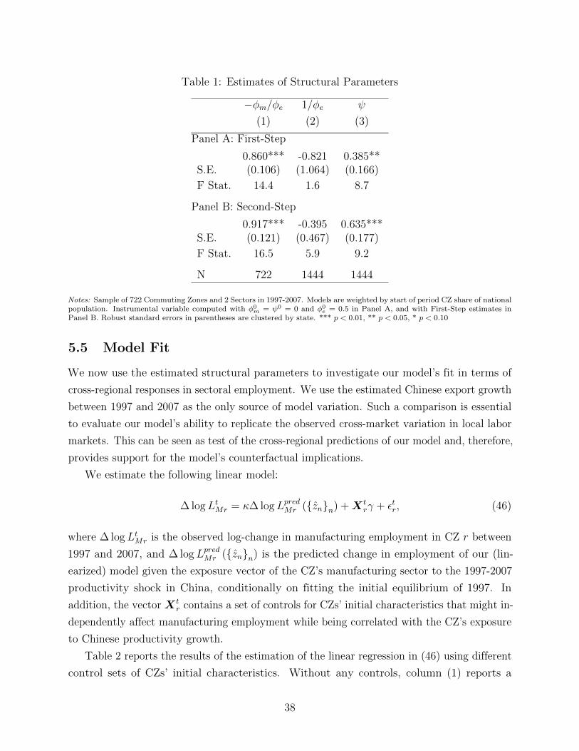
Table 1: Estimates of Structural Parameters

−φm/φe 1/φe ψ

(1) (2) (3)

Panel A: First-Step

0.860*** -0.821 0.385**S.E. (0.106) (1.064) (0.166)

F Stat. 14.4 1.6 8.7

Panel B: Second-Step

0.917*** -0.395 0.635***S.E. (0.121) (0.467) (0.177)

F Stat. 16.5 5.9 9.2

N 722 1444 1444

Notes: Sample of 722 Commuting Zones and 2 Sectors in 1997-2007. Models are weighted by start of period CZ share of nationalpopulation. Instrumental variable computed with φ0

m = ψ0 = 0 and φ0e = 0.5 in Panel A, and with First-Step estimates in

Panel B. Robust standard errors in parentheses are clustered by state. *** p < 0.01, ** p < 0.05, * p < 0.10

5.5 Model Fit

We now use the estimated structural parameters to investigate our model’s fit in terms of

cross-regional responses in sectoral employment. We use the estimated Chinese export growth

between 1997 and 2007 as the only source of model variation. Such a comparison is essential

to evaluate our model’s ability to replicate the observed cross-market variation in local labor

markets. This can be seen as test of the cross-regional predictions of our model and, therefore,

provides support for the model’s counterfactual implications.

We estimate the following linear model:

∆ logLtMr = κ∆ logLpredMr (znn) +X trγ + εtr, (46)

where ∆ logLtMr is the observed log-change in manufacturing employment in CZ r between

1997 and 2007, and ∆ logLpredMr (znn) is the predicted change in employment of our (lin-

earized) model given the exposure vector of the CZ’s manufacturing sector to the 1997-2007

productivity shock in China, conditionally on fitting the initial equilibrium of 1997. In

addition, the vector X tr contains a set of controls for CZs’ initial characteristics that might in-

dependently affect manufacturing employment while being correlated with the CZ’s exposure

to Chinese productivity growth.

Table 2 reports the results of the estimation of the linear regression in (46) using different

control sets of CZs’ initial characteristics. Without any controls, column (1) reports a

38

Table 2: Cross-Market Model Fit: Manufacturing Employment

Dependent variable: Log-change in manufacturing employment, 1997-2007(1) (2) (3) (4)

Predicted log-change in manuf. employment 7.52** 7.16** 6.44*** 6.84***(3.54) (2.99) (2.34) (2.08)

R2 0.05 0.17 0.22 0.27

Sector composition controls No Yes No Yes

Demographic controls No No Yes Yes

Notes: Sample of 722 Commuting Zones in 1997-2007. Models are weighted by start of period CZ share of national population.Sector composition controls in 1997: share of working-age population employed in manufacturing and share of spending onmanufacturing goods. Demographic controls in 1990: the population share with a college education, the foreign born populationshare, the employment rate of working-age women, and employmeny share in routine-intensive occupations. Robust standarderrors in parentheses are clustered by state. *** p < 0.01, ** p < 0.05, * p < 0.10

positive and statistically significant relationship between actual and predicted changes in

manufacturing employment across US CZs. This indicates that, in response to the Chinese

productivity shock, our model’s general equilibrium predictions are consistent with the

observed cross-region pattern of manufacturing employment changes.

In columns (2)–(4), we evaluate the robustness of this relationship to a set of demographic

and labor force measures that potentially eliminate confound effects. Column (2) reports a

similar coefficient when controlling for the CZ’s sector employment and spending composition

in 1997. This specification eases concerns that the China exposure variable may in part

be picking up an overall trend decline in US manufacturing. In column (3), we control for

the following set of CZ’s demographic characteristics in 1990: the population share with a

college education, the foreign born population share, the employment rate of working-age

women, and the employment share in routine intensive jobs (as defined in Autor and Dorn

(2013)). This specification shows that our results are robust to employment trends associated

with shocks emphasized by recent empirical papers, including immigration and technological

shocks. Finally, column (4) presents the estimation of the regression with the entire set of

controls. It is important to notice that this set of controls accounts for a significant share

of the cross-region variation in manufacturing employment growth in the period, as the R2

increases from 0.05 in column (1) to 0.27 in column (4).37

The methodology in Section 4 provides an interpretation for the estimated coefficient in

Table 2. Assumption 3c implies that it corresponds to the pass-through from the measured

productivity shock to the structural cost shocks in the model and, therefore, should be used

to adjust the shocks magnitude in the model’s predicted effect. Using this adjustment and

37Table 6 in Appendix B.3 shows that the structural estimates of Table 1 vary within their 95% with theinclusion of this additional set of controls.

39

the specification in column (4), we find that the difference between the CZs at the 25th and

the 75th percentiles of predicted response of manufacturing employment is 5.1 log-points.

Thus, our model’s differential effect has a similar magnitude to the one estimated by Autor,

Dorn, and Hanson (2013): in their preferred specification, the CZ at the 75th percentile of

import exposure experienced a manufacturing employment decline 4.5 log-points stronger

than the CZ in the 25th percentile.38

Moving beyond manufacturing employment, Panel A of Table 3 reports the estimation

of a version of the regression (46) with different labor market outcomes. Column (2) shows

that the predicted employment responses in non-manufacturing are also positively correlated

with the observed changes in non-manufacturing employment across CZs. Columns (3)–(4)

investigate the model’s cross-regional fit in terms of real wages. While we find a positive

and statistically significant relationship for the change in the manufacturing real wage, we

only obtain an imprecise relationship between the predicted and actual changes in non-

manufacturing real wage across CZs. Under the interpretation that the estimated coefficient

is the shock pass-through, the estimates in columns (1)–(4) of Panel A should be identical. In

fact, despite the difference in the point estimates, the large standard errors of the estimates

for the non-manufacturing sector imply that the estimated coefficients in Panel A are not

statistically different from each other at usual significance levels.

Finally, Panel B of Table 3 investigates the importance of different components of the

model’s predicted response to the trade shock. In particular, we analyze the differential

responses to the CZ’s exposure in terms of manufacturing revenue, log ηRMr, and consumption,

log ηCr . For both employment and real wage, we find that the impact of a manufacturing

revenue shock is positive and statistically significant in the manufacturing sector but non-

significant in the non-manufacturing sector. The exogenous increase in the CZ’s price index

has a negative impact on employment in both the manufacturing and the non-manufacturing

sectors. However, the coefficients are imprecisely estimated due to the lack of variation in

consumption exposure across US CZs. The next section investigates the contribution each of

these components to the model’s predicted responses in general equilibrium.39

38To compute the differential impact of import competition on manufacturing employment, we use theestimated coefficient of 4.231 reported in column (1) of Table 5.A in Autor, Dorn, and Hanson (2013). Thedifference of import exposure of the regions at the 75th and 25th percentiles in Autor, Dorn, and Hanson(2013) is 1.06, which multiplied by the 4.231 yields a predicted differential impact of 4.5 log-points. In theOnline Appendix B.3.3, we show that we closely replicate the estimated cross-regional employment responsein Autor, Dorn, and Hanson (2013) using their shift-share exposure measure to Chinese import competitionin our sample of 31 manufacturing industries.

39The Online Appendix B.3.3 investigate cross-regional employment responses to alternative shift-sharemeasures of the CZ’s exposure to Chinese import competition. In particular, we find that these measures arenegatively correlated with manufacturing employment growth across CZs.

40

Table 3: Cross-Market Model Fit: Sector-level Outcomes

Dependent variable: Log-change in sector outcome, 1997-2007Employment Real Wage

Manuf. Non-manuf. Manuf. Non-manuf.(1) (2) (3) (4)

Panel A: Model’s general equilibrium prediction

Predicted log-change 6.84*** 16.03** 8.86** -4.18(2.08) (6.94) (3.35) (12.49)

Panel B: CZ ’s shock exposure

Manufacturing revenue 1.05*** -0.17 1.64*** 0.12(0.31) (0.11) (0.36) (0.16)

Consumption cost -22.79 -9.12** -27.05 -2.76(13.73) (3.95) (18.68) (3.71)

Notes: Sample of 722 Commuting Zones in 1997-2007. Models are weighted by start of period CZ share of national population.All specifications include the set of baseline controls in column (4) of Table 2. Robust standard errors in parentheses areclustered by state. *** p < 0.01, ** p < 0.05, * p < 0.10

6 Quantifying the Effects of Global Shocks on Local

Labor Markets

Having estimated the deep elasticities that regulate cross-market links in our model, we now

investigate the general equilibrium responses of labor markets outcomes to global shocks.

To this end, we first present the reduced-form elasticity of local outcomes to the shock

exposure of different CZs. Then, we interact these elasticities with each CZ’s exposure to

global shocks and compute the predicted responses in general equilibrium. We focus on a

first-order approximation of these predicted effects to perform a decomposition into the direct

effect of local shock exposure as well as indirect effect of the exposure of other local labor

markets. More generally, besides these two effects, the model’s general equilibrium predicted

changes also entail a residual of the first-order approximation. We focus on the first-order

approximation of the models predictions to precisely measure the relative importance of the

direct and indirect effects.40

40The Online Appendix D.1 outlines the system of nonlinear equations that delivers the exact predictedchanges in labor market outcomes in the model. Using this system, we found that the residual of the first-orderapproximation was small relative to the predicted effects in many variations of our empirical exercise.

41

6.1 Reduced-Form Elasticities of Local Employment to Shock Ex-

posure

In this section, we use equation (25) to compute the reduced-form elasticities of local

employment to manufacturing shock exposure across US CZs. We report the reduced-form

elasticities of real wages in Table 11 in Appendix B.3. Specifically, we use the structural

parameters in Panel B of Table 1 to compute γRkr,Md and γCkr,Md in the observed equilibrium

of 1997. Table 4 presents the average of these reduced-form elasticities for the 722 CZs in

our sample.

Columns (1) and (2) report, respectively, the average effect of a shock in a CZ’s man-

ufacturing sector on that CZ’s employment in the manufacturing and non-manufacturing

sectors. Panel A shows that an exogenous decline of 1% in local manufacturing revenue

triggers an average decline of 0.18% in manufacturing employment and an average increase

of 0.02% in non-manufacturing employment. Thus, in response to negative shocks to the

local manufacturing sector, our model predicts manufacturing employment losses that are

not fully compensated by non-manufacturing employment growth. This prediction is in line

with the employment responses to Chinese import competition presented in Autor, Dorn,

and Hanson (2013).

Panel B shows that exogenous shocks to consumption costs also generate substantial

changes in employment in our model. If the cost of the consumption bundle of manufacturing

workers falls by 1%, then employment in manufacturing increases by 1.19%. These quantita-

tively important employment responses arise from two margins. First, because we normalize

the payoff of being in the home sector to one in every region, the exogenous change in the

price index has a first-order impact in the relative payoff of being non-employed in each CZ.

Second, a lower price index makes the CZ more attractive to workers from other CZs in the

country.

Turning to the cross-region indirect effects of shock exposure, column (3) evaluates

the average indirect impact of a shock in a CZ’s manufacturing sector on manufacturing

employment in all other CZs. Specifically, column (3) reports the averages∑

d 6=r lMdγRMd,Mr

and∑

d6=r lMdγCMd,Mr, where lMd ≡ LMd/

∑d′ LMd is the CZ’s share in national manufacturing

employment.41 The small coefficients in column (3) indicate that the indirect effect of any

specific CZ is very close to zero. In other words, CZs are approximately ‘‘small open

economies’’: local shock exposure does not trigger quantitatively large effects elsewhere.42

41Formally, the effect of a revenue shock in region r on aggregate manufacturing employment in other

regions is∂ log

∑d 6=r LMd

∂ log ηRr=∑d6=r

LMd∑d′ 6=r LMd′

∂ logLMd∂ log ηRr

=∑d6=r lMdγ

RMd,Mr.

42This feature of indirect effects being small is somewhat consistent with the findings in Caliendo, Parro,Rossi-Hansberg, and Sarte (2018b). In a quantitative spatial model featuring free mobility of workers across

42

Table 4: Reduced-Form Elasticities of Employment to Local Manufacturing Shock Exposure

Own region Other regionsγMr,Mr γNr,Mr

∑d6=r lMdγMd,Mr

∑d6=r γMr,Md

(1) (2) (3) (4)

Panel A: Employment elasticity to revenue exposure (γRMr,Md)

Avg. 0.1807 -0.0181 0.0002 -0.1730

Panel B: Employment elasticity to consumption exposure (γCMr,Md)

Avg. 1.1923 0.1255 -0.0006 -0.5296

Notes: Average reduced-form elasticity computed with equation (25) using the estimates in Panel B of Table 1 and the observedequilibrium in 1997. M denotes the manufacturing sector and N denotes the non-manufacturing sector.

In contrast, column (4) shows the average impact on a CZ’s manufacturing employment

of a common manufacturing shock to all other CZ’s – that is, the cross-region average of∑d 6=r γ

RMr,Md and

∑d6=r γ

CMr,Md. Column (4) in Panel A shows that if other CZs experience

a correlated shock that raises their revenue by 1%, then local employment in a typical CZ

falls by 0.17%. This negative reduced-form indirect effect follows from the positive impact of

higher revenue on the nominal wage of other CZs, which lowers local employment due to

out-migration and higher consumption costs.

The similarity between the magnitudes of the effects in columns (1) and (4) of Panel A

implies that indirect effects can partially offset local direct employment losses triggered by

Chinese import competition. These findings are directly connected to the theoretical results

shown in Theorem 1: a fully correlated shock across all markets has the potential to generate

sizable indirect effects, and thus offset the direct effect, despite small indirect effects of any

individual region.

Moreover, another compensating effect is given by the response of employment to con-

sumption exposure. In fact, the indirect effects in column (4) of Panel B are smaller than the

direct effect in column (1), suggesting that the direct consumption exposure is an important

force that offsets the direct revenue exposure. We will explore this relationship further in

Section 6.2.

Lastly, Figure 2 reports the entire distribution of the implied responses of local employment

to local shocks, for both revenue and consumption exposures. It illustrates that our model

yields heterogeneous reduced-form effects across US CZs – for instance, the standard deviation

regions and input-output linkages, they show that, following a state-specific productivity shock, the indirecteffect on other states is one order of magnitude smaller than the direct effect of the shock.

43

Figure 2: Distribution of reduced-form elasticities, Manufacturing Employment

Notes: Average reduced-form elasticity computed with equation (25) using the estimates in Panel B of Table 1 and the observedequilibrium in 1997. M denotes the manufacturing sector and N denotes the non-manufacturing sector.

of the direct revenue elasticity γRMr,Mr is 0.045. Our framework also features rich heterogeneity

in the indirect effects of a local shocks on other regions. In fact, the distribution of indirect

effects in Figure 2 suggests that indirect effects across CZs are as heterogeneous as the direct

effects – for instance, the standard deviation of the indirect revenue elasticity is 0.042. In

the following section, we will further explore the implications of such heterogeneity for the

impact of global shocks on US labor markets.43

6.2 Impact of Global Shocks on US Local Labor Markets

We conclude this section with a quantification of the differential and aggregate effects of

global shocks on sectoral employment across US CZs. We decompose these effects into

components related to the direct response to local shock exposure and the indirect response

to the exposure of other CZs in the country. We first evaluate the impact on CZs in the

US of the same China export shock we have used in the estimation, and then we conduct a

number of robustness exercises.

43Monte, Redding, and Rossi-Hansberg (2018) show that commuting flows across counties generatesvariation in the reduced-form response of local employment to local shocks. However, our focus is on themagnitude and dispersion of the indirect reduced-form responses of local employment to shocks in otherregions of the country.

44

Figure 3: Predicted Change in Manufacturing Employment, China shock

Notes: The figure on the left reports the scatter plot of the general equilibrium response of manufacturing employmentagainst the predicted revenue exposure and against the sum of the predicted revenue and consumption exposures. It alsodisplays the average (across CZs) of the general equilibrium response (horizontal line), revenue exposure (black line), revenueand consumption exposure (red line). The figure on the right reports the scatter plot of the general equilibrium responseagainst the predicted revenue exposure, and against the sum of predicted (domestic) direct and indirect effects from revenueand consumption exposures, computed using Proposition . It also displays the average (across CZs) of the general equilibriumresponse (horizontal line), revenue exposure (black line), domestic direct and indirect effects (red line).

6.2.1 China Export Shock

We quantify the importance of local shock exposure in revenue and consumption for the

model’s predicted employment responses. To this end, we plot the general equilibrium

employment response following the China export shock against alternative partial equilibrium

exposure measures.44 The graph on the left of Figure 3 reports the relationship between the

general equilibrium predictions of our model, ∆ logLpredkr (z), and the revenue exposure in

manufacturing, i.e. ∆ log ηRMr (z) , and the consumption exposure, i.e. ∆ log ηCMr (z). The

graph on the right, instead, displays the (domestic) direct and indirect effects.

We first take a look at the general equilibrium predicted responses of manufacturing

employment. Figure 3 shows that there is a large degree of heterogeneity in the employment

responses of US CZs. For the majority of the CZs, which account for 66% of the US

population, manufacturing employment falls due to Chinese import competition. In these

44Specifically, we denote each exposure measure by m, with m = GE representing our baseline generalequilibrium model. For each m, we compare predictions using the following linear regression:

∆ logLGEMr (τ) = αm + ρm∆ logLmMr (τ) + emMr,

where ∆ logLmMr (τ) is the shock exposure in manufacturing employment according to measure m. We thencompute the partial-equilibrium employment responses of exposure m as ρm∆ logLmMr (τ), with ρm being thecoefficient estimated in the equation above.

45

CZs, the average decline in manufacturing real wage is 1.16%. In contrast, 33% of the

population lives in CZs that experience an expansion in manufacturing employment, with

an average real wage gain of 1.09%. By combining winning and losing CZs, we obtain a

small aggregate impact of rising Chinese import competition: on average, manufacturing

employment falls by only 0.51%, while real wages decline by 0.064%. These small aggregate

effects of the China shock are similar to the findings reported in a number of recent structural

quantitative papers - e.g. Hsieh and Ossa (2016), Lee (2015), Galle, Rodriguez-Clare, and Yi

(2017), Adao, Costinot, and Donaldson (2017), and Caliendo, Dvorkin, and Parro (2018a).

Interestingly, non-manufacturing employment absorbs part of displaced workers due to

Chinese import competition, due to the reallocation of workers across sectors and the positive

employment impact of lower good prices. Overall, non-manufacturing employment falls only

in 13% of the CZs, and aggregate non-manufacturing employment increases by 0.9%.

A striking feature of the scatter plots in Figure 3 is the tight fit of the cross-regional

predictions of the partial-equilibrium measures. The revenue exposure alone, in particular,

is able to capture a large variation in the predicted employment effect across US CZs, and

on average it entails a decline in manufacturing employment of 6.47% due to the loss in

competitiveness from the China shock. The consumption exposure, on the other hand,

typically shifts upward the responses of CZs employment, due to the lower consumption costs

of Chinese goods. The consumption exposure accounts for half the difference between the

‘‘average’’ effect of revenue exposure and the general equilibrium predicted effect. Also, note

that the consumption exposure does not have substantial cross-regional variation, and this

explains the imprecise estimates in Table 3.

Another feature of the scatter plots is that most points are above the 45o degree line:

the partial-equilibrium predicted employment declines tend to be stronger than the total

general equilibrium responses. This arises because the partial-equilibrium measures ignore

the offsetting indirect effects triggered by the common component of the shock exposure –

i.e., the combined effect in column (4) of Table 4. In fact, the scatter plots on the right of

Figure 3 highlight that the indirect effects coming from other US commuting zones shift up

manufacturing employment, due to cheaper goods available from other regions negatively

affected by the China shock. On average, indirect effects offset about half of the negative

response of the revenue exposure.

In sum, while the revenue exposure accounts for most of the cross-regional variation in

the manufacturing employment responses, the consumption exposure offsets around half of

the average effect of ∆ log ηRMr, which implies, together with the offsetting impact of the

indirect effects from other CZs, an aggregate effect of the China shock of approximately zero.

46

6.2.2 Robustness

In this section we investigate the robustness of our empirical results to different specifications

of the model. We first study how the relationship between the shock exposure and general

equilibrium effect of the China shock is affected by labor linkages across markets. Figure 7 in

Appendix B.4 shows that shutting down the migration and agglomeration elasticities does

not substantially alter the fit of the local exposures to the general equilibrium response of

manufacturing employment. It does, however, affect their magnitudes. In fact, while the

average predicted effect is still close to zero, the average revenue and consumption exposures

are smaller than in the baseline. This is consistent with Theorem 1, which shows that labor

linkages across markets amplify the response of employment to shocks.

Second, we investigate how our main findings are affected by our assumption about the

unemployment margin. In particular, with the same parameters as in the baseline, we feed

the China export shock in a version of our empirical model that does not feature the home

sector. Figure 8 shows that, even without this margin of labor reallocation, the relationship

between local exposures and general equilibrium responses is very similar to the baseline

model.

Finally, we examine the response of local labor markets following a bilateral trade cost

shock. Specifically, starting from the labor market equilibrium in 2007, we revert US import

trade costs with Mexico and Canada back to what they were in 1993, the year before NAFTA

was implemented. We use the gravity structure of our model and the assumption that trade

costs are symmetric, as in Head and Ries (2001), to recover the change in trade costs from

observed changes in trade shares.45 Figure 9 shows that, despite the different nature of the

shock, the fit of the revenue and consumption exposure is similar to the one for the China

export shock, although the magnitudes are typically smaller than in the baseline.

7 Conclusions

We propose an integrated treatment for estimating the effect of economic shocks in the

world economy on local labor markets. Our analysis offers a bridge between quantitative

general equilibrium models and estimates of differential responses across markets. As in

45Imposing symmetric trade costs, our gravity model implies that

τn,Mi,kU =

(ˆxn,Mi,U

ˆxn,Mi,i·

ˆxn,MU,i

ˆxn,MU,U

)− 12χn

,

where i ∈ (Canada,Mexico), U stands for US, and n is each of the 31 industries within the manufacturingsector M . We use country-sector-level trade data from UN Comtrade for 1993 and 2007 to compute the tradeshares in the equation above.

47

quantitative structural approaches, we evaluate the general equilibrium effect of economic

shocks on each region. We show that this response has two components: the direct impact

of local shock exposure and the indirect effect of the shock exposure of other markets. By

providing a thorough theoretical characterization of these effects and a model-consistent way

to measure local shock exposure, we can exploit credible quasi-experimental variation, as in

recent empirical papers. We use such variation to estimate the deep elasticities governing

cross-market links and evaluate the model’s reduced-form predictions regarding changes in

outcomes across local labor markets. Our results quantify the role of spatial links in shaping

the factual and counterfactual responses of labor markets to international trade shocks.

Several interesting avenues for future research emerge from our study. Extensions of our

Generalized Spatial Model offer different measures of shock exposure that can be computed

using richer data. Furthermore, as our approach is flexible in specifying functional forms for

the cross-market links, finer micro-data can leverage on the MOIV methodology to improve on

the precision of estimated parameters. More importantly, our approach, easily implementable

with a simple GMM procedure, can be used for the estimation of structural parameters in a

wide class of general equilibrium models.

48

References

Acemoglu, D., Autor, D., Dorn, D., Hanson, G. H., Price, B., 2016. Import competition and

the great us employment sag of the 2000s. Journal of Labor Economics 34 (S1), S141--S198.

Acemoglu, D., Restrepo, P., 2017. Robots and jobs: Evidence from us labor markets. Tech.

rep., National Bureau of Economic Research, Inc.

Adao, R., 2015. Worker heterogeneity, wage inequality, and international trade: Theory and

evidence from brazil. Unpublished paper, MIT.

Adao, R., Costinot, A., Donaldson, D., 2017. Nonparametric counterfactual predictions

in neoclassical models of international trade. The American Economic Review 107 (3),

633--689.

Ahlfeldt, G. M., Redding, S. J., Sturm, D. M., Wolf, N., 2015. The economics of density:

Evidence from the berlin wall. Econometrica 83 (6), 2127--2189.

Allen, T., Arkolakis, C., 2014. Trade and the topography of the spatial economy. The

Quarterly Journal of Economics 129 (3), 1085--1140.

Allen, T., Arkolakis, C., Li, X., 2015. Optimal city structure. Yale University, mimeograph.

Allen, T., Arkolakis, C., Takahashi, Y., 2018. Universal gravity. Tech. rep., Mimeo North-

western and Yale University.

Allen, T., Donaldson, D., 2018. The geography of path dependence. Tech. rep., mimeo.

Altonji, J. G., Card, D., 1991. The effects of immigration on the labor market outcomes of

less-skilled natives. In: Immigration, Trade, and the Labor Market. University of Chicago

Press, pp. 201--234.

Anderson, J. E., 1979. A theoretical foundation for the gravity equation. American Economic

Review 69 (1), 106--116.

Arkolakis, C., Costinot, A., Donaldson, D., Rodrıguez-Clare, A., 2017. The elusive pro-

competitive effects of trade.

Arkolakis, C., Costinot, A., Rodrıguez-Clare, A., 2012. New trade models, same old gains?

American Economic Review 102 (1), 94--130.

49

Armington, P. S., 1969. A theory of demand for products distinguished by place of production.

International Monetary Fund Staff Papers 16, 159--178.

Arrow, K. J. K. J., Hahn, F. H., 1971. General competitive analysis. Tech. rep.

Autor, D., Dorn, D., 2013. The growth of low-skill service jobs and the polarization of the us

labor market. The American Economic Review 103 (5), 1553--1597.

Autor, D., Dorn, D., Hanson, G. H., 2013. The china syndrome: Local labor market effects

of import competition in the united states. The American Economic Review 103 (6),

2121--2168.

Autor, D. H., Dorn, D., Hanson, G. H., Song, J., 2014. Trade adjustment: Worker-level

evidence. The Quarterly Journal of Economics 129 (4), 1799--1860.

Balistreri, E. J., Hillberry, R. H., Rutherford, T. F., 2010. Trade and welfare: Does industrial

organization matter? Economics Letters 109 (2), 85--87.

Bartelme, D., 2018. Trade costs and economic geography: evidence from the us. Work. Pap.,

Univ. Calif., Berkeley.

Bartelme, D., Costinot, A., Donaldson, D., Rodriguez-Clare, A., 2017. Sector-level economies

of scale: Estimation using trade data.

Bartik, T. J., 1991. Who benefits from state and local economic development policies?

Beraja, M., Hurst, E., Ospina, J., 2016. The aggregate implications of regional business cycles.

Tech. rep., National Bureau of Economic Research.

Berry, S., 1994. Estimating discrete-choice models of product differentiation. RAND Journal

of Economics 25 (2), 242--262.

Berry, S., Gandhi, A., Haile, P., 2013. Connected substitutes and invertibility of demand.

Econometrica 81 (5), 2087--2111.

Berry, S., Levinsohn, J., Pakes, A., 1999. Voluntary export restraints on automobiles:

Evaluating a trade policy. American Economic Review, 400--430.

Berry, S. T., Haile, P. A., 2014. Identification in differentiated products markets using market

level data. Econometrica 82 (5), 1749--1797.

Blanchard, O., Katz, L. F., 1992. Regional evolutions, brooking papers on economic activity.

Economic Studies Program, The Brookings Institution 23 (1), 76.

50

Bryan, G., Morten, M., 2015. Economic development and the spatial allocation of labor:

Evidence from indonesia. Manuscript,Stanford University.

Burstein, A., Morales, E., Vogel, J., 2016. Changes in between-group inequality: computers,

occupations, and international trade. Tech. rep., mimeo, September 13.

Bustos, P., Caprettini, B., Ponticelli, J., 2016. Agricultural productivity and structural

transformation: Evidence from brazil. American Economic Review 106 (6), 1320--1365.

Caliendo, L., Dvorkin, M., Parro, F., 2018a. Trade and labor market dynamics: General

equilibrium analysis of the china trade shock. Tech. rep., mimeo.

Caliendo, L., Parro, F., 2014. Estimates of the trade and welfare effects of nafta. The Review

of Economic Studies.

Caliendo, L., Parro, F., Rossi-Hansberg, E., Sarte, P.-D., 2018b. The impact of regional and

sectoral productivity changes on the us economy. Tech. Rep. 1.

Chamberlain, G., 1987. Asymptotic efficiency in estimation with conditional moment restric-

tions. Journal of Econometrics 34 (3), 305--334.

Chetty, R., Guren, A., Manoli, D., Weber, A., 2013. Does indivisible labor explain the

difference between micro and macro elasticities? a meta-analysis of extensive margin

elasticities. NBER Macroeconomics Annual 27 (1), 1--56.

Ciccone, A., 2002. Agglomeration effects in europe. European Economic Review 46 (2),

213--227.

Comin, D. A., Lashkari, D., Mestieri, M., 2015. Structural change with long-run income and

price effects. Tech. rep., National Bureau of Economic Research.

Costinot, A., Donaldson, D., Komunjer, I., 2011. What goods do countries trade? a quantita-

tive exploration of ricardo’s ideas. The Review of Economic Studies, rdr033.

Costinot, A., Rodriguez-Clare, A., 2013. Trade theory with numbers: Quantifying the

consequences of globalization. Tech. rep., National Bureau of Economic Research.

Cravino, J., Sotelo, S., 2017. Trade induced structural change and the skill premium. Tech.

rep., National Bureau of Economic Research.

Dekle, R., Eaton, J., Kortum, S., 2007. Unbalanced trade. Tech. rep., National Bureau of

Economic Research.

51

Dix-Carneiro, R., Kovak, B. K., 2017. Trade liberalization and regional dynamics. American

Economic Review 107 (10), 2908--46.

Donaldson, D., Hornbeck, R., 2016. Railroads and american economic growth: A market

access approach. The Quarterly Journal of Economics, qjw002.

Eaton, J., Kortum, S., 2001. Technology, trade, and growth: A unified framework. European

Economic Review 45 (4-6), 1741--1780.

Eaton, J., Kortum, S., 2002. Technology, geography and trade. Econometrica 70 (5), 1741--

1779.

Eckert, F., 2018. Growing apart: Tradable services and the fragmentation of the us economy.

Eckert, F., Peters, M., 2018. Spatial structural change. Tech. rep., mimeo.

Ethier, W. J., 1982a. Decreasing costs in international trade and frank graham’s argument

for protection. Econometrica: Journal of the Econometric Society, 1243--1268.

Ethier, W. J., 1982b. National and international returns to scale in the modern theory of

international trade. American Economic Review 72 (3), 389--405.

Faber, B., Gaubert, C., 2016. Tourism and economic development: Evidence from mexico’s

coastline. Tech. rep., National Bureau of Economic Research.

Feenstra, R., 1994. New product varieties and the measurement of international prices.


Fujita, M., Krugman, P., Venables, A. J., 1999. The Spatial Economy: Cities, Regions, and

International Trade. MIT Press, Boston, Massachussetts.

Galle, S., Rodriguez-Clare, A., Yi, M., 2017. Slicing the pie: Quantifying the aggregate and

distributional effects of trade. Tech. rep., National Bureau of Economic Research.

Handbury, J., Weinstein, D. E., 2014. Goods prices and availability in cities. The Review of

Economic Studies 82 (1), 258--296.

Handley, K., Limao, N., 2017. Policy uncertainty, trade, and welfare: Theory and evidence

for china and the united states. American Economic Review 107 (9), 2731--83.

Head, K., Mayer, T., 2013. Gravity equations: Workhorse, toolkit, and cookbook. Centre for

Economic Policy Research.

52

Head, K., Ries, J., 2001. Increasing returns versus national product differentiation as an

explanation for the pattern of u.s.-canada trade. American Economic Review 91 (4),

858--876.

Heckman, J. J., Lance, L., Taber, C., 1998. General-equilibrium treatment effects: A study

of tuition policy. American Economic Review 88 (2), 381--386.

Helpman, E., 1998. The size of regions. Topics in Public Economics. Theoretical and Applied

Analysis, 33--54.

Herrendorf, B., Rogerson, R., Valentinyi, A., 2013. Two perspectives on preferences and

structural transformation. American Economic Review 103 (7), 2752--89.

Hornbeck, R., Moretti, E., 2018. Who benefits from productivity growth? direct and indirect

effects of local tfp growth on wages, rents, and inequality. Tech. rep., National Bureau of

Economic Research.

Hsieh, C.-T., Ossa, R., 2016. A global view of productivity growth in china. Journal of

international Economics 102, 209--224.

Kim, R., Vogel, J., 2018. Trade and inequality across local labor markets: The margins of

adjustment.

Kline, P., Moretti, E., 2014. Local economic development, agglomeration economies and the

big push: 100 years of evidence from the tennessee valley authority. Quarterly Journal of

Economics 129, 275--331.

Kortum, S., 1997. Research, patenting, and technological change. Econometrica 65 (6),

1389--1419.

Kovak, B. K., 2013. Regional effects of trade reform: What is the correct measure of

liberalization? The American Economic Review 103 (5), 1960--1976.

Krugman, P., 1980. Scale economies, product differentiation, and the pattern of trade.


Krugman, P., 1991. Increasing returns and economic geography. The Journal of Political

Economy 99 (3), 483--499.

Krugman, P., Venables, A. J., 1995. Globalization and the inequality of nations. Quarterly

Journal of Economics 110 (4), 857--880.

53

Kucheryavyy, K., Lyn, G., Rodrıguez-Clare, A., 2016. Grounded by gravity: A well-behaved

trade model with industry-level economies of scale. Tech. rep., National Bureau of Economic

Research.

Lee, E., 2015. Trade, inequality, and the endogenous sorting of heterogeneous workers. Tech.

rep., mimeo.

Li, Y.-T., Chen, F.-B., Wang, D.-F., 2009. New lower bounds on eigenvalue of the hadamard

product of an m-matrix and its inverse. Linear Algebra and its applications 430 (4),

1423--1431.

Lucas, R. E., Rossi-Hansberg, E., 2003. On the internal structure of cities. Econometrica

70 (4), 1445--1476.

Mas-Colell, A., Whinston, M. D., Green, J. R., 1995. Microeconomic Theory. Oxford Univer-

sity Press, Oxford, UK.

McFadden, D., 1980. Econometric models for probabilistic choice among products. Journal of

Business, S13--S29.

Mian, A., Sufi, A., 2014. What explains the 2007--2009 drop in employment? Econometrica

82 (6), 2197--2223.

Monte, F., Redding, S. J., Rossi-Hansberg, E., 2018. Commuting, migration, and local

employment elasticities. Tech. Rep. 12.

Moretti, E., 2011. Local labor markets. In: Handbook of labor economics. Vol. 4. Elsevier,

pp. 1237--1313.

Moretti, E., 2013. Real wage inequality. American Economic Journal: Applied Economics

5 (1), 65--103.

Muendler, M., 2017. Trade, technology, and prosperity: An account of evidence from a

labor-market perspective.

Nakamura, E., Steinsson, J., 2014. Fiscal stimulus in a monetary union: Evidence from us

regions. The American Economic Review 104 (3), 753--792.

Nakamura, E., Steinsson, J., 2018. Identification in macroeconomics. Journal of Economic

Perspectives 32 (3), 59--86.

Newey, W. K., McFadden, D., 1994. Large sample estimation and hypothesis testing. Hand-

book of econometrics 4, 2111--2245.

54

Newey, W. K., Powell, J. L., 2003. Instrumental variable estimation of nonparametric models.

Econometrica 71 (5), 1565--1578.

Petrin, A., 2002. Quantifying the benefits of new products: The case of the minivan. Journal

of political Economy 110 (4), 705--729.

Pierce, J. R., Schott, P. K., 2016a. The surprisingly swift decline of us manufacturing

employment. The American Economic Review 106 (7), 1632--1662.

Pierce, J. R., Schott, P. K., 2016b. Trade liberalization and mortality: Evidence from us

counties. Tech. rep., National Bureau of Economic Research.

Redding, S., Sturm, D., 2008. The costs of remoteness: Evidence from german division and

reunification. American Economic Review 98 (5), 1766--1797.

Redding, S., Venables, A. J., 2004. Economic geography and international inequality. Journal

of international Economics 62 (1), 53--82.

Redding, S. J., 2016. Goods trade, factor mobility and welfare. Journal of International

Economics 101, 148--167.

Redding, S. J., Rossi-Hansberg, E., 2016. Quantitative spatial economics. Tech. rep., National

Bureau of Economic Research.

Reynaert, M., Verboven, F., 2014. Improving the performance of random coefficients demand

models: the role of optimal instruments. Journal of Econometrics 179 (1), 83--98.

Roback, J., 1982. Wages, rents, and the quality of life. The Journal of Political Economy,

1257--1278.

Rosen, S., 1979. Wage-based indexes of urban quality of life. Current issues in urban economics

3, 324--345.

Rosenzweig, M. R., Wolpin, K. I., 2000. Natural ”natural experiments” in economics. Journal

of Economic Literature 38 (4), 827--874.

Simonovska, I., Waugh, M. E., 2014. Trade models, trade elasticities, and the gains from

trade. Tech. rep., National Bureau of Economic Research.

Sposi, M., 2018. Evolving comparative advantage, sectoral linkages, and structural change.

Journal of Monetary Economics.

Tolbert, C. M., Sizer, M., 1996. Us commuting zones and labor market areas.

55

Topalova, P., 2010. Factor immobility and regional impacts of trade liberalization: Evidence

on poverty from india. American Economic Journal: Applied Economics 2 (4), 1--41.

Wang, Z., Wei, S.-J., Yu, X., Zhu, K., 2018. Re-examining the impact of trading with china

on local labor markets: A supply chain perspective. Tech. rep.

Wolpin, K. I., 2013. The limits of inference without theory. MIT Press.

Wooldridge, J. M., 2010. Econometric analysis of cross section and panel data. MIT press.

56

A Proofs

A.1 Proof of Proposition 1

To establish the existence of equilibrium, consider the following system of equilibrium equations:

Fi(p∗jj) = 0.

We use the following two results regarding existence and uniqueness of equilibrium prices.

Lemma 1. [Mas-Colell, Whinston, and Green (1995) 17.C.1] Suppose that F (·) is a functiondefined for every p ∈ RN++ such that F (·) is (i) differentiable, (ii) homogeneous of degree 0, (iii)

satisfies Walras’ law,∑N

i=1 piFi(p) = 0 for all p, and (iv) there exists a s such that Fi(p) < s forevery p,and (v) if pn → p with pj = 0 for some j, miniFi(pn) → −∞. Then, p∗ ∈ RN++ exists.

Lemma 2. [Arrow and Hahn (1971) T.9.12 (p. 234)] Suppose that F (·) satisfies the conditions in

Lemma 1, and denote fij(p) ≡ ∂Fi(p)∂pj

. Assume that, for all p∗ ∈ RN+ with F (p∗) = 0, (i) fij(p∗) > 0

and (ii) ∃hi(p∗)Ni=1 0 such that hi(p∗)fii(p

∗) >∑

j 6=i,m |fij(p∗)|hj(p∗) for all i = 1, ..., N .

Then, p∗ ∈ RN++ is unique.

To establish the result, notice that (w∗, p∗) is an equilibrium with positive employment every-where if, and only if,

Λi(w∗, p) = 0

whereΛi(w, p) ≡ 1− p

wiτiΨi(Φ(w, p)) ∀i = 1, ..., N

ΛN+1(w, p) =N∑i=1

[τiΨi(Φ(w, p))− wip

].

To establish uniqueness, we verify the conditions of Lemmas 1 and 2. Notice that our function isan excess supply function, i.e. the negative of an excess demand function considered by Mas-Colell,Whinston, and Green (1995)

1. Continuity: By assumption, Ψi(Φ(w, p)) is differentiable, so Λi(w, p) is also continuous.

2. Homogeneous of Degree Zero: Consider (w, p) and (bw, bp) with b > 0. Both vectors implythe same vector of real wages, ωi = wi/p = bwi/bp, so Φ(bw, bp) = Φ(w, p) and Λi(bw, bp) =Λi(w, p).

3. Walras’ law: For any (w, p),

N∑i=1

wiΛi(w, p) + pΛN+1(w, p) =N∑i=1

[wi − pτiΨi(Φ(w, p))] +N∑i=1

[pτiΨi(Φ(w, p))− wi] = 0,

where the last equality follows from the zero profit condition.

4. Bounded from above: Because Ψi(.) ≥ 0, Λi(w, p) ≤ 1 for every i = 1, ..., N . GivenAssumption 1 the function Ψi(.) is bounded above, Ψi(.) < Ψ and ΛN+1(w, p) <

∑i τiΨ.

57

5. Limit: Consider a sequence (wn, pn)→ (w, p). If limn→∞wni = 0 for some i, then for every n

mini′

Λi′(w

n, pn)≤ 1− p

wiτiΨi(Φ(wn, pn).

We assume that limn→∞Ψiwni

=∞ for all i if limn→∞wni = 0. These two combined imply that

limn→∞min

Λi(wn, pn)

= −∞.

6. Conditions on the Jacobian: Notice that

∂Λi∂wi

=p

w2i

τiΨi(Φ(w, p))

(1− ∂Ψi(Φ(w, p))

∂wi

wiΨi(Φ(w, p))

)=

p

w2i

τiΨi(Φ(w, p))λii (ω) .

∂Λi∂wj

=p

wiwjτiΨi(Φ(w, p))

(−∂Ψi(Φ(w, p))

∂wj

wjΨi(Φ(w, p))

)=

p

wiwjτiΨi(Φ(w, p))λij (ω)

Immediately, Assumption 1(i) implies that ∂Λi∂wi

> 0. Assumption 1(ii) implies that there existshi ≡ hi(ω) such that

hiλii >∑j 6=i|λij |hj ,

which is equivalent to

(hiwi)p

w2i

τiΨi(Φ(w, p))λii >∑j 6=i| p

wiwjτiΨi(Φ(w, p))λij |(hjwj)

By defining hi ≡ hiwi, we have that hi∂Λi∂wi

>∑

j 6=i |∂Λi∂wi|hj .

A.2 Proof of Theorem 1

Part 1. λij(ω0)

= λ1[i=j] implies that λ(ω0)

= λI and, therefore, β = λ−1I.

Part 2. λij(ω0)

= λ1[i=j] − λj implies that λ(ω0)

= λI − Iλ′, where I is a vector of ones and

λ ≡ λjj . We guess and verify that λ(ω0)−1

= λ−1I +[λ(λ−

∑j λj

)]−1Iλ′.

λ(ω0)λ(ω0)−1

= I + λ[λ(λ−

∑j λj

)]−1Iλ′ − λ−1Iλ′ −

[λ(λ−

∑j λj

)]−1I(λ′I)λ′

= I + λ[λ(λ−

∑j λj

)]−1Iλ′ − λ−1Iλ′ −

[λ(λ−

∑j λj

)]−1 (∑j λj

)Iλ′

= I −[λ−1 −

[λ(λ−

∑j λj

)]−1 (λ−

∑j λj

)]Iλ′ = I

where the second equality follows from λ′I =

∑j λj ..

Part 3. This is an extension of Lemma 2.1 in Li, Chen, and Wang (2009). We first show that|βkj |/hk < |βjj |/hj for all k and j. Suppose that there is p 6= j such that |βpj |/hp ≥ |βkj |/hk forall k. By definition of inverse matrix, we have that

∑k λpkβkj = 0 for p 6= j, which implies that

λppβpj = −∑

k 6=p λpkβkj . Thus,

58

λpp|βpj | = |∑k 6=p

λpkβkj | ≤∑k 6=p|λpk||βkj | ≤

∑k 6=p|λpk||βpj |

hkhp

⇒ hpλpp ≤∑j 6=p|λpk|hk,

which contradicts Assumption 1(ii).To establish the result, notice that, by definition, λiiβij = −

∑k 6=i λikβkj for every j 6= i. Thus,

λii|βij | ≤∑k 6=i|λik||βkj | <

∑k 6=i|λik||βjj |

hkhj

⇒ |βij ||βjj |

<

∑k 6=i |λik|hkλiihj

.


We start by replicating the argument in Proposition 1 to establish that, for each pi/Pi, thereexists a unique real wage vector satisfying labor market module in (18). To this end, ω∗ satisfies(18) if, and only if, ω∗ ≡ p∗ω∗ and p∗ solve the following system,

Λi(ω∗, p∗) = 0

where

Λi(ω, p) ≡ 1− p

ωi

piPi

Ψi

(Φ

(ω

p

))∀i = 1, ..., N

ΛN+1(ω, p) =N∑i=1

[piPi

Ψi

(Φ

(ω

p

))− ωi

p

].

Under Assumption 1, Proposition 1 implies that the solution (ω∗, p∗) is a unique solution up toa scalar. Thus, ω∗ = ω∗/p is unique for each vector of relative competitiveness, pi/Pii. Thus,the local labor market module in (18) defines the real wage vector as function of the relativecompetitiveness vector and, because Pi = Pi(τoipoo), of the vector of production costs,p. Thus,we can write

ω = Ω(p),

where, by the implicit function theorem,[∂ logωi∂ log pj

]i,j

≡ Ω = β(I − x).

We then substitute ω = Ω(p) into the trade module in (19) to write the equilibrium as thesolution of

Γi(p) = 0 ∀i

where pj ≡ τojpoo and

Γi(p) ≡ Ψi (Φ (Ω(p))) Φi (Ω(p))− 1

pi

∑j

Xij

(pj)

Ψj (Φ (Ω(p))) Φj (Ω(p)) pj .

To establish uniqueness, we verify the conditions of Lemmas 1 and 2 as in the proof of Proposition1.

1. The function Γi(p) is differentiable because all functions are differentiable by assumption.

59

2. To show that the system is homogeneous of degree zero, recall that Pi(·) is homogeneous ofdegree one, which implies that κpi/Pi(τoiκpoo) = pi/Pi(τoipoo) and Ω(κp) = Ω(p). SinceXij(·) is homogeneous of degree zero, it is straight forward to verify that Γi(κp) = Γi(p).

3. To verify that Walras’ law holds, note that∑i piΓi(p) =

∑i piΨi (Φ (Ω(p))) Φi (Ω(p))−

∑j

[∑iXij

(pj)]

Ψj (Φ (Ω(p))) Φj (Ω(p)) pj=

∑i piΨi (Φ (Ω(p))) Φi (Ω(p))−

∑j pjΨj (Φ (Ω(p))) Φj (Ω(p))

= 0

4. Given Assumptions 1 and 2 the excess supply system has the following upper bound:

Γi(p) < Ψi (Φ (Ω(p))) Φi (Ω(p)) < ΨΦ

5. Let p be a real price vector with pi = 0 for some i. Notice that because of the upper boundsconditions on Assumptions 1 and 2 we have

0 ≤ limpn→p

Ψi (Φ (Ω(p))) Φi (Ω(p)) ≤ ΨΦ.

Making use of the limiting conditions in Assumption 2 if limn→∞ pni = 0, then for every n

also notice that

mini′Γi′(p) ≤ NΨΦ− 1

pi

∑j

Xij

(pj)

Ψj (Φ (Ω(p))) Φj (Ω(p)) pj .

Then, limn→+∞XijΦjΨj

pni=∞ for some j and thus limpn→p Γi(p) = −∞.

6. We now establish diagonal dominance of the excess supply system at any equilibrium pricevector. To this end, notice that

∂Γi(p)∂ log po

= Ψi (Φ (Ω(p))) Φi (Ω(p))[∑

d ψid∑

d φddΩdo +∑

d φidΩdo

]+ 1

pi

∑j Xij

(τojpoo

)Ψj (Φ (Ω(p))) Φj (Ω(p)) pj (1[i = o]− 1[j = o])

− 1pi

∑j Xij

(pj)

Ψj (Φ (Ω(p))) Φj (Ω(p)) pj

(χoij +

∑d ψid

∑d φddΩdo +

∑d φjdΩdo

)Define Yi ≡ Ψi (Φ (Ω(p))) Φi (Ω(p)) and yij ≡ 1

piYiXij

(τojpoo

)Ψj (Φ (Ω(p))) Φj (Ω(p)) pj

Thus,

1Yi

∂(Γi(p))∂ log po

=∑

d ψid∑

d φdd∂ logωd∂ log po

+∑

d φjd∂ logωd∂ log po

+∑

j yij (1[i = o]− 1[j = o])

−∑

j yij

[χoij +

∑d ψid

∑d φdd

∂ logωd∂ log po

+∑

d φjd∂ logωd∂ log po

].

Notice that∑

j yij = 1 for every equilibrium price. Hence,[1Yi

∂Γi(p)∂ log po

]i,o

= ψφΩ + φΩ + I − y − χ− y[ψφΩ + φΩ

]= I − χ− y +

(I − y

) (ψ + I

)φΩ

= I − χ− y + µΩ= I − χ− y + µβ(I − x)= γ(p)

60

This implies that ∂Γi(p)∂po

= Yipoγio. Immediately, by Assumption 2(i), ∂Γi(p)

∂pi= Yi

piγii > 0.

Assumption 2(ii) implies that there exists hi ≡ hi(p) such that

hiγii >∑j 6=i|γij |hj ,

which is equivalent to

(hipi)Yipiγii >

∑j 6=i| Yipjγij |(pjhj).

By defining hi ≡ hipi, we have that hi∂Γi(p)∂pi

>∑

j 6=i |∂Γi(p)∂pj|hj .


In this proof, we simplify the notation by writing log ηR(τ ) = log ηR and log ηC(τ ) = log ηC .

Part 1: Small Open Economy. Under the assumption of segmented markets, the equilibriumsatisfies the following system of equations:

log Li = φ

(− log ηCi + log pi −

∑o

x0oi log po + ψ log Li

),

∑o

(1[o=i] − y0

io − χio)

log po = log ηRi − (1 + ψ)∑j

(1[j=i] − y0

ij

)log Lj .

Consider a shock that only affects a set of small open economies d ∈ I: log τij = 0 and log ζi ifi 6= d and j 6= d. By the definition, we have that x0

di = y0id = 0 all i 6= d, which implies that

log ηCi ≡ x0di log τdi = 0, and log ηRi ≡ χ

∑d

y0jd

(x0id log τid

)= 0.

Thus, for all i 6= d, log ηCi = log ηRi = 0 and the system above becomes

log Li = φ

(log pi −

∑o

x0oi log po + ψ log Li

),

∑o

(1[o=i] − y0

io − χio)

log po = −(1 + ψ)∑j

(1[j=i] − y0

ij

)log Lj .

This implies that we can solve the problem recursively. The system above is satisfied iflog pi = log Li = 0 for all i 6= d. For each small open economy d, we have to solve the followingsystem:

log Ld = φ(− log ηCd + (1− xdd) log pd + ψ log Ld

)(1− y0

dd − χdd)

log pd = log ηRd −(1− y0

dd

)(1 + ψ) log Ld.

Define β ≡ (1− φψ)−1. Rearranging the first expression in this system, we get

log Ld = βφ(− log ηCd +

(1− x0

dd

)log pd

), (47)

61

Substituting (47) into the second equation in the system above, we get that(1− y0

dd − χdd)

log pd = log ηRd −(1− y0

dd

)(1 + ψ)βφ

(− log ηCd +

(1− x0

dd

)log pd

)Define αdd ≡

(1− y0

dd − χdd + (1 + ψ)βφ(1− y0

dd

) (1− x0

dd

))−1. Thus

log pd = αdd(log ηRd +

(1− y0

dd

)(1 + ψ)βφ log ηCd

). (48)

By combining expressions (47) and (48),

log ωd = βαRdd log ηRd − βαCdd log ηCd

where αRdd ≡(1− x0

dd

)αdd and αCdd ≡

[1− αRdd

(1− y0

dd

)(1 + ψ)βφ

]. Notice that if the small open

economies are symmetric with xdd = x and ydd = y, then αRdd = αR and αCdd = αC .

Part 2. We start by establishing the following lemma.

Lemma. Take any two matrices a and b such that aij = a1[i=j] − aj and bij = b1[i=j] − bj. Then,

c ≡ ab has entries with cij = ab1[i=j] − baj − abj + bj∑

d ad = c1[i=j] − cj.

Proof.

cij =∑d

aidbdj =∑d

(a1[i=d] − ad

) (b1[d=j] − bj

)= ab1[i=j] −

[abj +

∑d

ad

(b1[d=j] − bj

)]

Using this lemma, notice that, under Assumption 3,φij = φ1[i=j] − φj and ψij = ψ1[i=j] − ψj ,which implies that λij = λ1[i=j] − λj . Thus, Part 2 of Proposition 1 immediately implies that

log ω = β(

log p− log P), (49)

whereβij = λ−11[i=j] + λ−1λj with λ ≡ (λ−

∑j

λj)λ.

We now characterize the matrix γ, which is defined as

γ ≡ I − χ− y +(I − y

) (I + ψ

)φβ(I − x

).

With frictionless trade (τij = 1 for all i and j), pij = τipi, xij = xi = Xi(τopoo) and yji = yi =wjLj/(

∑dwdLd) for all j. Since trade balance holds at the world economy, wiLi = xi

∑j wjLj and

xi = yi for all i. The gravity trade structure in Assumption 3 implies that χoij = −χ(1[o=i] − xo)and, therefore,

χij ≡∑d

yidχjid = −χ1[i=j] + χ∑d

yidxj = −χ1[i=j] + χxj

Thus, χ = −χ(I − x), implying that

γ ≡ (1 + χ)(I − x

)+ κ

(I − x

)where

κ ≡(I − x

) (I + ψ

)φβ.

62

Let us define a ≡ I − x and b ≡(I + ψ

)φβ such that κ ≡ ab. By the lemma above, we can

write bij ≡ κ1[i = j]− bj . This implies that κij = κ (1[i = j]− xj)− bj +∑

d xdbj = κ (1[i = j]− xj).Hence,

κ = κ(I − x

)and

γ ≡ (1 + χ)(I − x

)+ κ

(I − x

) (I − x

).

Since∑

d

(1[i=d] − xd

) (1[d=j] − xj

)= 1[i=j]−xj −xj +xj

∑d xd = 1[i=j]−xj , we have that(

I − x) (I − x

)=(I − x

)and

γ ≡ (1 + χ+ κ)(I − x

). (50)

By defining γ ≡ 1 + χ + κ and γj = γxj , we have that γij = γ1[i = j] − γj . Thus, Part 2 ofProposition 1 implies that, for every i 6= m,

log pi =1

γhi +

1

γ

∑j 6=m

xjxm

hj

with h = log ηR + κ log ηC and, therefore,

hi = log ηRi + κ log ηCi − κ∑j

xj log ηCj .

For i 6= m,

log pi =1

γ

(log ηRi + κ log ηCi

)+

1

γ

∑j 6=m

xjxm

(log ηRj + κ log ηCj

)− 1

xm

κ

γ

∑j

xj log ηCj (51)

To write an equivalent expression for i = m with log pm = 0, notice that∑j xj log ηRj = −χ

∑j xj

[∑d yd

(log τjd − log ηCd

)]−χ∑

d yd

[∑j xj log τjd − log ηCd

]−χ∑

d yd[log ηCd − log ηCd

]= 0

This implies that log pm = 0 can be written as

log pm =1

γ

(log ηRm + κ log ηCm

)+

1

γ

∑j 6=m

xjxm


)− 1

xm

κ

γ

∑j

xj log ηCj . (52)

Finally, the change in the price index is log Pi = log ηCi +∑

j xj log pj , which in combinationwith (51) and (52) yields

log Pi = log ηCi +1

γ

∑j 6=m

xjxm


)− 1− xm

xm

κ

γ

∑j

xj log ηCj

and, therefore,

63

log pi − log Pi =1

γlog ηRi −

(1− κ

γ

)log ηCi −

κ

γ

∑j

xj log ηCj .

Finally, the combination of this expression and equation (49) yields

log ωi = 1γ

[1λ log ηRi + 1

λ

∑j λj log ηRj

]−

[1λ

(1− κ

γ

)log ηCi + 1

λ

∑j

((1− κ

γ

)λj + κ

γλxj

)log ηCj

],

where λ ≡ (λ−∑

j λj)λ.

A.5 Proof of Expression (31)

The asymptotic variance of the GMM estimator for any function Hi(· ) is

V (H) =(E[Hi

(zt,W 0

)Gi])−1

(E[Hi

(zt,W 0

)eiei′Hi

(zt,W 0

)′]) (E[Hi

(zt,W 0

)Gi])−1′

(53)where Gi ≡ E

[∇θei(θ)|zt,W 0

].

The asymptotic variance of the Optimal IV estimator in (31) is

V (H∗) = E[Gi′ (Ω (zt,W 0

))−1Gi

](54)

with Ω(zt,W 0

)= E

[ei(θ)ei(θ)′)|zt,W 0

].

We now show that V (H)− V (H∗) is positive semi-definite for any Hi(· ):

V (H)− V (H∗) =(E[HtiG

ti

])−1(E[(Hti eti

) (Hti eti

)′]) (E[HtiG

ti

])−1 ′ −(E[Gti′Ω−1Gti

])−1

=(E[HtiG

ti

])−1(E[(Hti eti

) (Hti eti

)′]− E [HtiG

ti

] (E[Gti′Ω−1Gti

])−1E[HtiG

ti

]′) (E[HtiG

ti

])−1.

Let us define

U ti ≡ Hti eti − E

[(Hti eti

) (Gt′i Ω−1eti

)′] (E[Gti′Ω−1Gti

])−1Gt′i Ω−1eti,

which implies that

E[U tiU

ti′] = E

[(Hti eti

) (Hti eti

) ′]− E[HtiG

ti](E[GtiΩ

−1Gti])−1

E[HtiG

ti]′.

Therefore,

V (H)− V (H∗) =(E[HtiG

ti

])−1 (E[U tiU

ti′]) (E [Ht

iGti

])−1′.

Since E[U tiU

ti′] is positive semi-definite, V (H)− V (H∗) is also positive semi-definite. Therefore,

the asymptotic variance is minimized at H∗.


From Proposition 2,

E[∆ logLt|zt,W 0

]≈ γR(θ)E

[log ηR(τ t)|zt,W 0

]− γC(θ)E

[log ηC(τ t)|zt,W 0

]. (55)

64

Because of Assumption 3c, equation (21) implies that

E[log ηCi (τ )|zt,W 0

]=

∑j x

0jiE

[log τji|zt,W 0

]= κ

∑j x

0ji log zji

= κ log ηCi (z|W 0),

and equation (22) implies that

E[log ηRi (τ )|zt,W 0

]=

∑j

∑o y

0ijχoijE

[log τoi|zt,W 0

]= κ

∑j

∑o y

0ijχoij log zoi

= κ log ηRi (z|W 0).

By plugging these two expressions into equation (55), we have that

E[∆ logLt|zt,W 0

]≈ ∆ logL

(zt,W 0|θ

). (56)

The combination of (32) and (56) yields the first-order approximation in (33) for the optimal IVin (31).


We use the strategy in Section 6.1 of Newey and McFadden (1994) to establish asymptotic propertiesof two-step estimators. To this end, we define the joint moment equation for the two estimatingsteps:

(θ2, θ1

)≡ arg min

θ2,θ1

∑i,t

vti (θ2,θ1)

′∑i,t

vti (θ2,θ1)

(57)

where

vti (θ2,θ1) ≡[HMOIVi (zt,W 0|θ1)eti(θ2) HMOIV

i (zt,W 0|θ0)eti(θ1)]

We have that(θ2, θ1

)p→ (θ,θ), with an asymptotic variance given by

V ar(θ2, θ1

)=(G′Ω−1G

)−1

where G ≡[∇(θ2,θ1)v

ti (θ2,θ1)

]and Ω ≡ E

[(vti (θ2,θ1)

) (vti (θ2,θ1)

)′].

Define hti ≡ HMOIVi (zt,W 0|θ)eti(θ) and hti ≡ HMOIV

i (zt,W 0|θ0)eti(θ). Thus, G and Ω aregiven by

Ω = E

[htih

t′i htih

t′i

htiht′i htih

t′i

]and G =

[G G1

0 G2

]where

G ≡ E[HMOIVi (zt,W 0|θ)∇θeti(θ)

]G1 ≡ E

[∇θHMOIV

i (zt,W 0|θ)eti(θ)]

65

G2 ≡ E[HMOIVi (zt,W 0|θ0)∇θeti(θ)

].

By Assumption 3c, any function of(zt,W 0

)is orthogonal to eti (θ), which implies that G1 = 0.

Thus,(G′Ω−1G

)−1is block diagonal and the marginal distribution of θ2 is asymptotically normal

with variance

V ar(θ2

)=(G′Ω−1G

)−1,

which is equivalent to the asymptotic distribution of the Optimal IV in (54).

66

Spatial Linkages, Global Shocks, and Local Labor Markets ...ka265/research/LaborSupplyTrade/Adao...

Documents

Transcript of Spatial Linkages, Global Shocks, and Local Labor Markets ...ka265/research/LaborSupplyTrade/Adao...