Spatial Equilibration in Transport Networks

Anna Nagurney

Department of Finance and Operations Management

Isenberg School of Management

University of Massachusetts

Amherst, Massachusetts 01003

December 2002; revised January 2003

Submitted to the Handbook on Transport Geography and Spatial Systems

Editors: P. Stopher, D. Hensher, K. Haynes, and K. F. Button

1

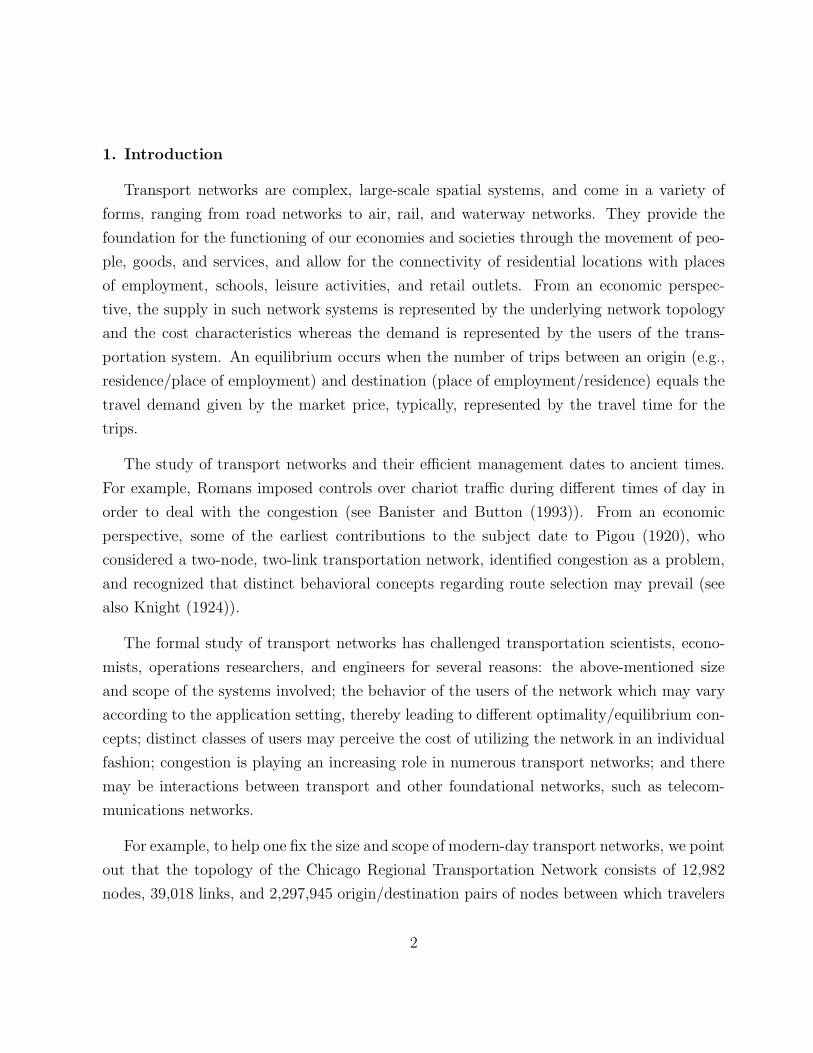
1. Introduction

Transport networks are complex, large-scale spatial systems, and come in a variety of

forms, ranging from road networks to air, rail, and waterway networks. They provide the

foundation for the functioning of our economies and societies through the movement of peo-

ple, goods, and services, and allow for the connectivity of residential locations with places

of employment, schools, leisure activities, and retail outlets. From an economic perspec-

tive, the supply in such network systems is represented by the underlying network topology

and the cost characteristics whereas the demand is represented by the users of the trans-

portation system. An equilibrium occurs when the number of trips between an origin (e.g.,

residence/place of employment) and destination (place of employment/residence) equals the

travel demand given by the market price, typically, represented by the travel time for the

trips.

The study of transport networks and their efficient management dates to ancient times.

For example, Romans imposed controls over chariot traffic during different times of day in

order to deal with the congestion (see Banister and Button (1993)). From an economic

perspective, some of the earliest contributions to the subject date to Pigou (1920), who

considered a two-node, two-link transportation network, identified congestion as a problem,

and recognized that distinct behavioral concepts regarding route selection may prevail (see

also Knight (1924)).

The formal study of transport networks has challenged transportation scientists, econo-

mists, operations researchers, and engineers for several reasons: the above-mentioned size

and scope of the systems involved; the behavior of the users of the network which may vary

according to the application setting, thereby leading to different optimality/equilibrium con-

cepts; distinct classes of users may perceive the cost of utilizing the network in an individual

fashion; congestion is playing an increasing role in numerous transport networks; and there

may be interactions between transport and other foundational networks, such as telecom-

munications networks.

For example, to help one fix the size and scope of modern-day transport networks, we point

out that the topology of the Chicago Regional Transportation Network consists of 12,982

nodes, 39,018 links, and 2,297,945 origin/destination pairs of nodes between which travelers

2

choose their routes (cf. Bar-Gera (1999)), whereas in the Southern California Association

of Governments’ model there are 25,428 nodes, 99,240 links, 3,217 origin/destination pairs,

and 6 distinct classes of users (Wu, Florian, and He (2000)).

Road congestion results in $100 billion in lost productivity in the US alone with the figure

being approximately $150 billion in Europe with the number of cars expected to increase by

50 percent by 2010 and to double by 2030 (see Nagurney (2000) and the references therein).

Moreover, in many of today’s transport networks, the “noncooperative” behavior of users

aggravates the congestion problem. For example, in the case of urban transport networks,

travelers select their routes from an origin to a destination so as to minimize their own travel

cost or travel time, which although optimal from a user’s perspective (user-optimization)

may not be optimal from a societal one (system-optimization) where a decision-maker or

central controller has control of the flows on the network and seeks to allocate the flows so

as to minimize the total cost in the network. Hence, before making any policy decisions on

transport networks one needs to identify the underlying behavioral mechanisms regarding

route selection.

This point is richly illustrated through the famous Braess (1968) paradox example, in

which it is assumed that the underlying behavioral principle is that of user-optimization

and travelers select their routes accordingly. In the Braess network, the addition of a new

road with no change in travel demand results in all travelers in the network incurring a

higher travel cost. Hence, they are all worse off after the addition of the new road. Actual

practical instances of such a phenomenon have been identified in New York City and in

Stuttgart, Germany. In 1990, 42nd Street in New York was closed for Earth Day, and the

traffic flow in the area improved (see Kolata (1990)). In Stuttgart, in turn, a new road was

added to the downtown, but the traffic flow worsened and, following complaints, the new

road was torn down (cf. Bass (1992)). Interestingly, this phenomenon is also relevant to

telecommunications networks (see Korilis, Lazar, and Orda (1999)) and, specifically, to the

Internet (cf. Cohen and Kelly (1990)).

The coupling of transportation networks with telecommunication networks through elec-

tronic commerce, notably, through business to business and business to consumer commerce,

and through Intelligent Transportation Systems is further transforming the economic land-

3

scape and affecting the movement of people, goods, services, as well as information (see

Nagurney and Dong (2002a)). Telecommunication networks are assuming many of the char-

acteristics of transport networks, including large-size, noncooperative behavior of the users,

as well as congestion. In fact, telecommunication networks, in a sense, may be interpreted

as transport networks on which the flows correspond to information (rather than vehicles,

etc.).

In this chapter, we recall the foundations of the equilibration of transport networks and

trace the evolution of modeling frameworks for their study. The exposition is meant to

be accessible to practitioners and to students, as well as to researchers in transport and

to those interested in related network topics. Technical derivations and further supporting

documentation are referred to in the citations. Further useful material and a supplementary

chronological perspective of developments on this topic can be found in the review articles

of Florian (1986), Boyce, LeBlanc, and Chon (1988), and Florian and Hearn (1995); in the

books by Beckmann, McGuire, and Winsten (1956), Sheffi (1985), Patriksson (1994), Ran

and Boyce (1996), Nagurney (1999, 2000), Nagurney and Dong (2002a), and in the volumes

edited by Florian (1976, 1984), Volmuller and Hamerslag (1984), Lesort (1996), Marcotte

and Nguyen (1998), Gendreau and Marcotte (2002), and Taylor (2002).

4

2. Basic Decision-Making Concepts and Models

Half a century ago, Wardrop (1952) explicitly recognized alternative possible behaviors

of users of transport networks, notably, urban transport networks and stated two principles,

which are commonly named after him:

First Principle: The journey times of all routes actually used are equal, and less than

those which would be experienced by a single vehicle on any unused route.

Second Principle: The average journey time is minimal.

The first principle corresponds to the behavioral principle in which travelers seek to (uni-

laterally) determine their minimal costs of travel whereas the second principle corresponds

to the behavioral principle in which the total cost in the network is minimal.

Beckmann, McGuire, and Winsten (1956) were the first to rigorously formulate these

conditions mathematically, as had Samuelson (1952) in the framework of spatial price equi-

librium problems in which there were, however, no congestion effects. Specifically, Beckmann,

McGuire, and Winsten (1956) established the equivalence between the traffic network equilib-

rium conditions, which state that all used paths connecting an origin/destination (O/D) pair

will have equal and minimal travel times (or costs) (corresponding to Wardrop’s first prin-

ciple), and the Kuhn-Tucker (1951) conditions of an appropriately constructed optimization

problem, under a symmetry assumption on the underlying functions. Hence, in this case, the

equilibrium link and path flows could be obtained as the solution of a mathematical program-

ming problem. Their approach made the formulation, analysis, and subsequent computation

of solutions to traffic network problems based on actual transportation networks realizable.

Dafermos and Sparrow (1969) coined the terms user-optimized (U-O) and system-optimized

(S-O) transportation networks to distinguish between two distinct situations in which, re-

spectively, users act unilaterally, in their own self-interest, in selecting their routes, and

in which users select routes according to what is optimal from a societal point of view, in

that the total cost in the system is minimized. In the latter problem, marginal total costs

rather than average costs are equilibrated. The former problem coincides with Wardrop’s

first principle, and the latter with Wardrop’s second principle.

5

Table 1: Distinct Behavior on Transportation Networks

User-Optimization System-Optimization⇓ ⇓

Equilibrium Principle: Optimality Principle:User travel costs onused paths for each O/Dpair are equalized andminimal.

Marginals of the totaltravel cost on used pathsfor each O/D pair areequalized and minimal.

See Table 1 for the two distinct behavioral principles underlying transportation networks.

The concept of “system-optimization” is also relevant to other types of “routing models” in

transportation, as well as in communications (cf. Bertsekas and Gallager (1992)), including

those concerned with the routing of freight and computer messages, respectively. Dafermos

and Sparrow (1969) also provided explicit computational procedures, that is, algorithms, to

compute the solutions to such network problems in the case where the user travel cost on a

link was an increasing (in order to handle congestion) function of the flow on the particular

link, and linear.

2.1 System-Optimization versus User-Optimization

In this section, the basic transport network models are first reviewed, under distinct

assumptions of their operation and distinct behavior of the users of the network. The models

are classical and are due to Beckmann, McGuire, and Winsten (1956) and Dafermos and

Sparrow (1969). In subsequent sections, we present more general models in which the user

link cost functions are no longer separable and are also asymmetric. For such models we also

provide the variational inequality formulations of the governing equilibrium conditions, since,

in such cases, the conditions can no longer be reformulated as the Kuhn-Tucker conditions

of a convex optimization problem.

For definiteness, and for easy reference, we present the classical system-optimized network

model in Section 2.1.1 and then the classical user-optimized network model in Section 2.1.2.

6

2.1.1 The System-Optimized Problem

Consider a general network G = [N ,L], where N denotes the set of nodes, and L the

set of directed links. Let a denote a link of the network connecting a pair of nodes, and

let p denote a path consisting of a sequence of links connecting an origin/destination (O/D)

pair. In transport networks, nodes correspond to origins and destinations, as well as to

intersections. Links, on the other hand, correspond to roads/streets in the case of urban

transportation networks and to railroad segments in the case of train networks. A path

in its most basic setting, thus, is a sequence of “roads” which comprise a route from an

origin to a destination. In the telecommunication context, however, nodes can correspond to

switches or to computers and links to telephone lines, cables, microwave links, etc. Note that

here we consider paths, rather than routes, since the former subsumes the latter. Moreover,

the network concepts presented here are sufficiently general to abstract not only transport

decision-making but also combined location-transport decision-making, which we return to

later. In addition, in the setting of supernetworks (see Nagurney and Dong (2002a)), a

path is viewed more broadly and need not be limited to a route-type decision but may, in

fact, correspond to not only transport but also to telecommunications decision-making, or a

combination thereof, as in the case of teleshopping and/or telecommuting.

Let Pω denote the set of paths connecting the origin/destination (O/D) pair of nodes

ω. Let P denote the set of all paths in the network and assume that there are J ori-

gin/destination pairs of nodes in the set Ω. Let xp represent the flow on path p and let fa

denote the flow on link a. The path flows on the network are grouped into the column vector

x ∈ RnP+ , where nP denotes the number of paths in the network. The link flows, in turn,

are grouped into the column vector f ∈ Rn+, where n denotes the number of links in the

network.

The following conservation of flow equation must hold:

fa =∑

p∈P

xpδap, ∀a ∈ L, (1)

where δap = 1, if link a is contained in path p, and 0, otherwise. Expression (1) states that

the flow on a link a is equal to the sum of all the path flows on paths p that contain (traverse)

link a.

7

Moreover, if one lets dω denote the demand associated with O/D pair ω, then one must

have that

dω =∑

p∈Pω

xp, ∀ω ∈ Ω, (2)

where xp ≥ 0, ∀p ∈ P ; that is, the sum of all the path flows between an origin/destination

pair ω must be equal to the given demand dω.

Let ca denote the user link cost associated with traversing link a, and let Cp denote the

user cost associated with traversing the path p. Assume that the user link cost function is

given by the separable function

ca = ca(fa), ∀a ∈ L, (3)

where ca is assumed to be continuous and an increasing function of the link flow fa in order

to model the effect of the link flow on the cost.

The total cost on link a, denoted by ca(fa), hence, is given by:

ca(fa) = ca(fa) × fa, ∀a ∈ L, (4)

that is, the total cost on a link is equal to the user link cost on the link times the flow on

the link. Here the cost is interpreted in a general sense. From a transportation engineering

perspective, however, the cost on a link is assumed to typically coincide with the travel time

on a link.

As noted earlier, in the system-optimized problem, there exists a central controller who

seeks to minimize the total cost in the network system, where the total cost is expressed as

∑

a∈Lca(fa), (5)

and the total cost on a link is given by expression (4).

The system-optimization problem is, thus, given by:

Minimize∑

a∈Lca(fa) (6)

8

subject to:∑

p∈Pω

xp = dω, ∀ω ∈ Ω, (7)

fa =∑

p∈P

xp, ∀a ∈ L, (8)

xp ≥ 0, ∀p ∈ P. (9)

The constraints (7) and (8), along with (9), are commonly referred to in network termi-

nology as conservation of flow equations. In particular, they guarantee that the flow in the

network, that is, the users (whether these are travelers or computer messages, for example)

do not “disappear from the network,” and, hence, are “conserved.”

The total cost on a path, denoted by Cp, is the user cost on a path times the flow on a

path, that is,

Cp = Cpxp, ∀p ∈ P, (10)

where the user cost on a path, Cp, is given by the sum of the user costs on the links that

comprise the path, that is,

Cp =∑

a∈Lca(fa)δap, ∀a ∈ L. (11)

In view of (8), one may express the cost on a path p as a function of the path flow variables

and, hence, an alternative version of the above system-optimization problem can be stated

in path flow variables only, where one has now the problem:

Minimize∑

p∈P

Cp(x)xp (12)

subject to constraints (7) and (9).

System-Optimality Conditions

Under the assumption of increasing user link cost functions, the objective function in the

S-O problem is convex, and the feasible set consisting of the linear constraints is also convex.

Therefore, the optimality conditions, that is, the Kuhn-Tucker conditions are: For each O/D

9

pair ω ∈ Ω, and each path p ∈ Pω, the flow pattern x (and link flow pattern f), satisfying

(7)–(9) must satisfy:

C ′p

= µω, if xp > 0≥ µω, if xp = 0,

(13)

where C ′p denotes the marginal of the total cost on path p, given by:

C ′p =

∑

a∈L

∂ca(fa)

∂fa

δap, (14)

evaluated in (13) at the solution and µω is the Largrange multiplier associated with constraint

(7) for that O/D pair ω.

Observe that conditions (13) may be rewritten so that there exists an ordering of the

paths for each O/D pair whereby all used paths (that is, those with positive flow) have

equal and minimal marginal total costs and the unused paths (that is, those with zero flow)

have higher (or equal) marginal total costs than those of the used paths. Hence, in the S-O

problem, according to the optimality conditions (13), it is the marginal of the total cost

on each used path connecting an O/D pair which is equalized and minimal (see also, e.g.,

Dafermos and Sparrow (1969)).

2.1.2 The User-Optimized Problem

We now describe the user-optimized network problem, also commonly referred to in the

transportation literature as the traffic assignment problem or the traffic network equilibrium

problem. Again, as in the system-optimized problem of Section 2.1.1, the network G =

[N ,L], the demands associated with the origin/destination pairs, as well as the user link

cost functions are assumed as given. Recall that user-optimization follows Wardrop’s first

principle.

Network Equilibrium Conditions

In the case of the user-optimization problem one seeks to determine the path flow pattern

x∗ (and the link flow pattern f ∗) which satisfies the conservation of flow equations (7), (8),

and the nonnegativity assumption on the path flows (9), and which also satisfies the network

equilibrium conditions given by the following statement. For each O/D pair ω ∈ Ω and each

10

path p ∈ Pω:

Cp

= λω, if x∗p > 0≥ λω, if x∗p = 0.

(15)

Hence, in the user-optimization problem there is no explicit optimization concept, since

now users of the transport network system act independently, in a noncooperative man-

ner, until they cannot improve on their situations unilaterally and, thus, an equilibrium is

achieved, governed by the above equilibrium conditions. Indeed, conditions (15) are simply

a restatement of Wardrop’s (1952) first principle mathematically and mean that only those

paths connecting an O/D pair will be used which have equal and minimal user costs. In (15)

the minimal cost for a given O/D pair is denoted by λω and its value is obtained once the

equilibrium flow pattern is determined.

Otherwise, a user of the network could improve upon his situation by switching to a

path with lower cost. User-optimization represents decentralized decision-making, whereas

system-optimization represents centralized decision-making. See also Table 1.

In order to obtain a solution to the above problem, Beckmann, McGuire, and Winsten

(1956) established that the solution to the equilibrium problem, in the case of user link cost

functions (cf. (3)) in which the cost on a link only depends on the flow on that link could

be obtained by solving the following optimization problem:

Minimize∑

a∈L

∫ fa

0ca(y)dy (16)

subject to:∑

p∈Pω

xp = dω, ∀ω ∈ Ω, (17)

fa =∑

p∈P

xpδap, ∀a ∈ L, (18)

xp ≥ 0, ∀p ∈ P. (19)

Note that the conservation of flow equations are identical in both the user-optimized

network problem (see (17)–(19)) and the system-optimized problem (see (7)–(9)). The be-

havior of the individual decision-makers termed “users,” however, is different. Users of the

11

network system, which generate the flow on the network now act independently, and are not

controlled by a centralized controller.

The objective function given by (16) is simply a device constructed to obtain a solution

using general purpose convex programming algorithms. It does not possess the economic

meaning of the objective function encountered in the system-optimization problem given

by (6), equivalently, by (12). Note that in the case of separable, as well as nonseparable

but symmetric (which we come back to later), user link cost functions the λω term in (15)

corresponds to the Lagrange multiplier associated with the constraint (17) for that O/D pair

ω. However, in the case of nonseparable and asymmetric functions there is no optimization

reformulation of the traffic network equilibrium conditions (15) and the λω term simply

reflects the minimum user cost associated with the O/D pair ω at the equilibrium.

3. Models with Asymmetric Link Costs

There has been much research activity in the past several decades in terms of both the

modeling and the development of methodologies to enable the formulation and computation

of more general traffic (and related) network equilibrium models. Examples of general models

include those that allow for multiple modes of transportation or multiple classes of users,

who perceive cost on a link in an individual way. In this section, we consider network models

in which the user cost on a link is no longer dependent solely on the flow on that link.

Assume that user link cost functions are now of a general form, that is, the cost on a link

may depend not only on the flow on the link but on other link flows on the network, that is,

ca = ca(f), ∀a ∈ L. (20)

In the case where the symmetry assumption exists, that is, ∂ca(f)∂fb

= ∂cb(f)∂fa

, for all links

a, b ∈ L, one can still reformulate the solution to the network equilibrium problem satisfy-

ing equilibrium conditions (15) as the solution to an optimization problem (cf. Dafermos

(1972), and the references therein), albeit, again, with an objective function that is arti-

ficial and simply a mathematical device. However, when the symmetry assumption is no

longer satisfied, such an optimization reformulation no longer exists and one must appeal to

variational inequality theory . Models of traffic networks with asymmetric cost functions are

12

important since they allow for the formulation, qualitative analysis, and, ultimately, given

the state-of-the-art, solution to problems in which the cost on a link may depend on the flow

on another link in a different way than the cost on the other link depends on that link’s flow.

Such a generalization allows for the more realistic treatment of intersections, two-way links,

multiple modes of transport as well as distinct classes of users of the network.

Indeed, it was in the domain of such traffic network equilibrium problems that the theory

of finite-dimensional variational inequalities realized its earliest success, beginning with the

contributions of Smith (1979) and Dafermos (1980). For an introduction to the subject,

as well as applications ranging from traffic network and spatial price equilibrium problems

to financial equilibrium problems, see the book by Nagurney (1999). Below we present

variational inequality formulations of both fixed demand and elastic demand traffic network

equilibrium problems.

The system-optimization problem, in turn, in the case of nonseparable (cf. (20)) user link

cost functions becomes (see also (6)–(9)):

Minimize∑

a∈Lca(f), (21)

subject to (7)–(9), where ca(f) = ca(f) × fa, ∀a ∈ L.

The system-optimality conditions remain as in (13), but now the marginal of the total

cost on a path becomes, in this more general case:

C ′p =

∑

a,b∈L

∂cb(f)

∂faδap, ∀p ∈ P. (22)

Variational Inequality Formulations of Fixed Demand Problems

As mentioned earlier, in the case where the user link cost functions are no longer sym-

metric, one cannot compute the solution to the U-O, that is, to the network equilibrium,

problem using standard optimization algorithms. We emphasize, again, that such general

cost functions are very important from an application standpoint since they allow for asym-

metric interactions on the network. For example, allowing for asymmetric cost functions

permits one to handle the situation when the flow on a particular link affects the cost on

13

another link in a different way than the cost on the particular link is affected by the flow on

the other link.

First, the definition of a variational inequality problem is recalled. For further back-

ground, theoretical formulations, derivations, and the proofs of the results below, see the

books by Nagurney (1999) and by Nagurney and Dong (2002a) and the references therein.

We provide the variational inequality of the network equilibrium conditions in path flows as

well as in link flows.

Specifically, the variational inequality problem (finite-dimensional) is defined as follows:

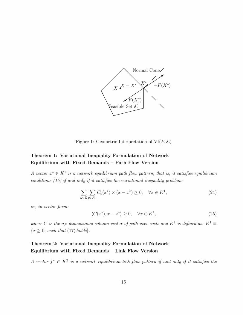
Definition 1: Variational Inequality Problem

The finite-dimensional variational inequality problem, VI(F,K), is to determine a vector

X∗ ∈ K such that

〈F (X∗), X −X∗〉 ≥ 0, ∀X ∈ K, (23)

where F is a given continuous function from K to RN , K is a given closed convex set, and

〈·, ·〉 denotes the inner product in RN .

Variational inequality (23) is referred to as being in standard form. Hence, for a given

problem, typically an equilibrium problem, one must determine the function F that enters

the variational inequality problem, the vector of variables X, as well as the feasible set K.

The variational inequality problem contains, as special cases, such well-known problems

as systems of equations, optimization problems, and complementarity problems. Thus, it is

a powerful unifying methodology for equilibrium analysis and computation.

A geometric interpretation of the variational inequality problem VI(F,K) is given in

Figure 1. In particular, F (X∗) is “orthogonal” to the feasible set K at the point X∗.

14

AA

AA

AAA

@@

@@

@@

3

+

X∗

@@

@@

@@

Normal Cone

−F (X∗)

F (X∗)

X −X∗

Feasible Set K

X

Figure 1: Geometric Interpretation of VI(F,K)

Theorem 1: Variational Inequality Formulation of Network

Equilibrium with Fixed Demands – Path Flow Version

A vector x∗ ∈ K1 is a network equilibrium path flow pattern, that is, it satisfies equilibrium

conditions (15) if and only if it satisfies the variational inequality problem:

∑

ω∈Ω

∑

p∈Pω

Cp(x∗) × (x− x∗) ≥ 0, ∀x ∈ K1, (24)

or, in vector form:

〈C(x∗), x− x∗〉 ≥ 0, ∀x ∈ K1, (25)

where C is the nP -dimensional column vector of path user costs and K1 is defined as: K1 ≡x ≥ 0, such that (17) holds.

Theorem 2: Variational Inequality Formulation of Network

Equilibrium with Fixed Demands – Link Flow Version

A vector f ∗ ∈ K2 is a network equilibrium link flow pattern if and only if it satisfies the

15

variational inequality problem:

∑

a∈Lca(f

∗) × (fa − f ∗a ) ≥ 0, ∀f ∈ K2, (26)

or, in vector form:

〈c(f ∗), f − f ∗〉 ≥ 0, ∀f ∈ K2, (27)

where c is the n-dimensional column vector of link user costs and K2 is defined as: K2 ≡f | there exists anx ≥ 0 and satisfying (17) and (18).

Note that one may put variational inequality (25) into standard form (23) by letting

F ≡ C, X ≡ x, and K ≡ K1. Also, one may put variational inequality (27) into standard

form where now F ≡ c, X ≡ f , and K ≡ K2.

Alternative variational inequality formulations of a problem are useful in devising other

models, including dynamic versions, as well as for purposes of computation using different

algorithms. In Section 5, we describe the relationship between variational inequality for-

mulations and projected dynamical systems, in which the latter provides the disequilibrium

dynamics prior to the attainment of the equilibrium, as formulated via the former.

The theory of variational inequalities (see Kinderlehrer and Stampacchia (1980) and

Nagurney (1999)) allows one to qualitatively analyze the equilibrium patterns in terms of

existence, uniqueness, as well as sensitivity and stability of solutions, and to apply rigorous

algorithms for the numerical computation of the equilibrium patterns. Variational inequality

algorithms usually resolve the variational inequality problem into series of simpler subprob-

lems, which, in turn, are often optimization problems, which can then be effectively solved

using a variety of algorithms, including the aforementioned equilibration algorithms of Dafer-

mos and Sparrow (1969), which exploit network structure as well as the commonly used in

practice Frank-Wolfe (1956) algorithm (see also LeBlanc, Morlok, and Pierskalla (1975)). In

particular, projection methods as well as relaxation methods (see Dafermos (1980, 1982),

Florian and Spiess (1982), Nagurney (1984, 1999), and Patriksson (1994)) have been success-

fully applied to compute solutions to variational inequality formulations of traffic network

equilibrium problems.

We emphasize that the above network equilibrium framework is sufficiently general to also

16

formalize the entire transportation planning process (consisting of origin selection, or desti-

nation selection, or both, in addition to route selection, in an optimal fashion) as path choices

over an appropriately constructed abstract network or supernetwork. This was recognized

by Dafermos in 1976 (in the context of separable link cost functions) in her development of

such integrated traffic network equilibrium models in which location decisions are made si-

multaneous to transportation route decisions (see also Boyce (1980)). Further discussion can

be found in that reference as well as in the books by Nagurney (1999, 2000) and Nagurney

and Dong (2002a) who also developed more general models in which the costs (as described

above) need not be separable nor asymmetric.

It is worth noting that the presentation of the variational inequality formulations of

the fixed demand models given above was in the context of single mode (or single class)

transport networks. We emphasize, however, that in view of the generality of the functions

considered (cf. (20)), the modeling framework described above can also be adapted to

multimodal/multiclass problems in which there are multiple modes of transport available

and/or multiple classes of users, each of whom perceives the cost on the links of the network

in an individual manner. Dafermos in (1972) demonstrated how, through a formal model, a

multiclass traffic network could be cast into a single-class network through the construction

of an expanded (and, again, abstract) network consisting of as many copies of the original

network as there were classes. The application of such a transformation is also relevant to

telecommunication networks.

Also, we note that here the focus is on deterministic network equilibrium problems. Some

basic stochastic traffic network equilibrium models can be found in Sheffi (1985). Dial (1971)

is credited with developing the first stochastic route choice model. Daganzo and Sheffi (1977),

in turn, formulated a stochastic user-optimized traffic network model with route choice in

which the equilibrium criterion could be succinctly stated as no traveler can improve his or

her perceived travel time by unilaterally changing routes.

Finally, we emphasize that the dynamic models presented in Section 5 (although presented

in a deterministic framework) have been analyzed qualitatively using tools from stochastic

processes (cf. Dupuis and Nagurney (1993) and Nagurney and Zhang (1996).

17

Variational Inequality Formulations of Elastic Demand Problems

We now describe a general network equilibrium model with elastic demands due to Dafer-

mos (1982). Specifically, it is assumed that one has associated with each O/D pair ω in the

network a travel disutility function λω, where here the general case is considered in which

the disutility may depend upon the entire vector of demands, which are no longer fixed, but

are now variables, that is,

λω = λω(d), ∀ω ∈ Ω, (28)

where d is the J-dimensional column vector of the demands.

The notation, otherwise, is as described earlier, except that here we also consider user

link cost functions which are general, that is, of the form (20). The conservation of flow

equations (see also (1) and (2)), in turn, are given by

fa =∑

p∈P

xpδap, ∀a ∈ L, (29)

dω =∑

p∈Pω

xp, ∀ω ∈ Ω, (30)

xp ≥ 0, ∀p ∈ P. (31)

Hence, in the elastic demand case, the demands in expression (30) are now variables and

no longer given, as was the case for the fixed demand expression in (2).

Network Equilibrium Conditions in the Case of Elastic Demand

The network equilibrium conditions (see also (15)) now take on in the elastic demand

case the following form: For every O/D pair ω ∈ Ω, and each path p ∈ Pω, a vector of

path flows and demands (x∗, d∗) satisfying (30)–(31) (which induces a link flow pattern f ∗

through (29)) is a network equilibrium pattern if it satisfies:

Cp(x∗)

= λω(d∗), if x∗p > 0≥ λω(d∗), if x∗p = 0.

(32)

Equilibrium conditions (32) state that the costs on used paths for each O/D pair are equal

and minimal and equal to the disutility associated with that O/D pair. Costs on unutilized

18

paths can exceed the disutility. Condition (32) can be given an economic interpretation as

described in the first paragraph of the Introduction. Observe that in the elastic demand

model users of the network can forego travel altogether for a given O/D pair if the user

costs on the connecting paths exceed the travel disutility associated with that O/D pair. We

emphasize that this model, hence, allows one to ascertain the attractiveness of different O/D

pairs based on the ultimate equilibrium demand associated with the O/D pairs. In addition,

this model can also handle such situations as the equilibrium determination of employment

location and route selection, or residential location and route selection, or residential and

employment selection as well as route selection through the appropriate transformations via

the addition of links and nodes, and given, respectively, functions associated with the resi-

dential locations, the employment locations, and the network overall (cf. Dafermos (1976),

Nagurney (1999), and Nagurney and Dong (2002a)).

Also, we note that although the presentation of the elastic demand traffic network model

has been in the case of a single mode of transport or class of user one can readily (with an

accompanying increase in notation) explicitly introduce distinct modes to the above model

as follows. One needs only to introduce subscripts to denote modes/classes, redefine all of

the above vectors accordingly, and the conservation of flow equations, and state that (32)

then must hold for each mode/class. In other words, in equilibrium, the used paths for a

given mode and O/D pair must have minimal and equal user path costs, which in turn, must

be equal to the travel disutility for that mode and O/D pair at the equilibrium demand. Of

course, as described in the case of fixed demands, one can also have made as many copies as

there are modes on the network in which case the above single-modal but extended elastic

demand model would be equivalent to the multimodal one.

In the next two theorems, both the path flow version and the link flow version of the

variational inequality formulations of the network equilibrium conditions (32) are presented.

These are analogues of the formulations (24) and (25), and (26) and (27), respectively, for

the fixed demand model.

Theorem 3: Variational Inequality Formulation of Network

Equilibrium with Elastic Demands – Path Flow Version

19

A vector (x∗, d∗) ∈ K3 is a network equilibrium path flow pattern, that is, it satisfies equilib-

rium conditions (32) if and only if it satisfies the variational inequality problem:

∑

ω∈Ω

∑

p∈Pω

Cp(x∗) × (x− x∗) −

∑

ω∈Ω

λω(d∗) × (dω − d∗ω) ≥ 0, ∀(x, d) ∈ K3, (33)

or, in vector form:

〈C(x∗), x− x∗〉 − 〈λ(d∗), d− d∗〉 ≥ 0, ∀(x, d) ∈ K3, (34)

where λ is the J-dimensional vector of disutilities and K3 is defined as: K3 ≡ x ≥0, such that (30) holds.

Theorem 4: Variational Inequality Formulation of Network

Equilibrium with Elastic Demands – Link Flow Version

A vector (f ∗, d∗) ∈ K4 is a network equilibrium link flow pattern if and only if it satisfies

the variational inequality problem:

∑

a∈Lca(f

∗) × (fa − f ∗a ) −

∑

ω∈Ω

λω(d∗) × (dω − d∗ω) ≥ 0, ∀(f, d) ∈ K4, (35)

or, in vector form:

〈c(f ∗), f − f ∗〉 − 〈λ(d∗), d− d∗〉 ≥ 0, ∀(f, d) ∈ K4, (36)

where K4 ≡ (f, d), such that there exists anx ≥ 0 satisfying (29), (31)

Note that, under the symmetry assumption on the disutility functions, that is, if ∂λw

∂dω=

∂λω

∂dw, for all w, ω, in addition to such an assumption on the user link cost functions (see fol-

lowing (20)), one can obtain (see Beckmann, McGuire, and Winsten (1956)) an optimization

reformulation of the network equilibrium conditions (32), which in the case of separable user

link cost functions and disutility functions is given by:

Minimize∑

a∈L

∫ fa

0ca(y)dy −

∑

ω∈Ω

∫ dω

0λω(z)dz (37)

subject to: (29)–(31).

20

j

j

j

1

2

3?

a b

c

R

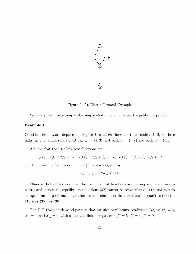
Figure 2: An Elastic Demand Example

We now present an example of a simple elastic demand network equilibrium problem.

Example 1

Consider the network depicted in Figure 2 in which there are three nodes: 1, 2, 3; three

links: a, b, c; and a single O/D pair ω1 = (1, 3). Let path p1 = (a, c) and path p2 = (b, c).

Assume that the user link cost functions are:

ca(f) = 5fa + 2fb + 15, cb(f) = 7fb + fa + 15, cc(f) = 3fc + fa + fb + 12,

and the disutility (or inverse demand) function is given by:

λω1(dω1) = −2dω1 + 114.

Observe that in this example, the user link cost functions are non-separable and asym-

metric and, hence, the equilibrium conditions (32) cannot be reformulated as the solution to

an optimization problem, but, rather, as the solution to the variational inequalities (33) (or

(34)), or (35) (or (36)).

The U-O flow and demand pattern that satisfies equilibrium conditions (32) is: x∗p1= 5,

x∗p2= 4, and d∗ω1

= 9, with associated link flow pattern: f ∗a = 5, f ∗

b = 4, f ∗c = 9.

21

The incurred user costs on the paths are: Cp1 = Cp2 = 96, which is precisely the value of

the disutility λω1 . Hence, this flow and demand pattern satisfies equilibrium conditions (32).

Indeed, both paths p1 and p2 are utilized and their user paths costs are equal to each other.

In addition, these costs are equal to the disutility associated with the origin/destination pair

that the two paths connect.

We note that the elastic demand model described above is related closely to the well-

known spatial price equilibrium models of Samuelson (1952), Takayama and Judge (1971),

and Florian and Los (1982). Indeed, as demonstrated by Dafermos and Nagurney (1985)

in the context of a single commodity, and, subsequently, by Dafermos (1986) in the case of

multiple commodities, spatial price equilibrium problems are isomorphic to traffic network

equilibrium problems over appropriately constructed networks. Hence, the well-developed

theory of traffic networks can be transferred to the study of commodity flows in the case of

spatial price equilibrium in which the equilibrium production, consumption, and commodity

trade flows are to be determined satisfying the equilibrium conditions that there will be a

positive flow (in equilibrium) of the commodity between a pair of supply and demand markets

if the supply price at the supply market plus the unit cost of transportation is equal to the

demand price at the demand market. A variety of such models (both static and dynamic)

and associated references can be found in the books by Nagurney (1999) and Nagurney and

Zhang (1996).

Although the focus of this paper is on transport network equilibrium models in an urban

setting, models of freight networks are closely related to those discussed above. Of course, one

must distinguish the behavior of the operators of such networks and model the competition

accordingly (see, e.g., Friesz and Harker (1985)).

4. Multiclass, Multicriteria Traffic Network Equilibrium Models

In this section, we describe multiclass, multicriteria network equilibrium models which

can serve as an alternative to multimodal traffic network equilibrium models. These models

are important since they allow for the individual weighting of distinct criteria associated with

decision-making on networks and especially transport networks. Moreover, such models have

been successful in formalizing decision-making surrounding transport/telecommunication

22

network tradeoffs as in the case of telecommuting versus commuting decision-making and

teleshopping versus shopping decision-making (cf. Nagurney and Dong (2002a, b, c), Nagur-

ney, Dong, and Mokhtarian (2002a, b)).

Multicriteria traffic network models were introduced by Quandt (1967) and Schneider

(1968) and explicitly consider that travelers may be faced with several criteria, notably,

travel time and travel cost, in selecting their optimal routes of travel. The ideas were

further developed by Dial (1979) who proposed an uncongested model and Dafermos (1981)

who introduced congestion effects and derived an infinite-dimensional variational inequality

formulation of her multiclass, multicriteria traffic network equilibrium problem, along with

some qualitative properties. The paper by Nagurney and Dong (2002b) provides a chronology

of citations, which highlights: the number of criteria treated by various authors, typically,

travel time and travel cost; whether or not these functions are allowed to be flow-dependent or

not, and the form (separable or general) handled. In addition, it notes the type of demand

considered, that is, fixed or elastic, and whether the demand is class-dependent, and, if

elastic, what form the demand functions take. Moreover, it provides the type of methodology

used in the formulation and analysis such as, for example, an optimization approach, a

finite-dimensional variational inequality approach, or infinite-dimensional approach, along

with whether the citation contains algorithmic contributions and/or qualitative ones. We

note that, in the case of infinite-dimensional variational inequality formulations, the number

of classes is, usually, infinite, whereas in the case of finite-dimensional formulations, the

number of classes is assumed to be finite. Additional citations, including literature exploring

multicriteria traffic models used in practice, may be found in the book chapter by Leurent

(1998).

In this section, for completeness, we recall the multiclass, multicriteria network equilib-

rium model with elastic demand developed by Nagurney and Dong (2002b). The model has

the following novel and what we believe are significant features:

1. It includes weights associated with the two criteria of travel time and travel cost which are

not only class-dependent but also, explicitly , link-dependent. Such weights may incorporate

such subjective factors as the relative safety or risk associated with particular links, the

relative comfort, or even the view.

23

2. It treats demand functions (rather than their inverses) which are very general and not

separable functions. Specifically, the demand associated with a class and origin/destination

(O/D) pair can depend not only on the travel disutility of different classes traveling between

the particular O/D pair but can also be influenced by the disutilities of the classes traveling

between other O/D pairs. Hence, the model has implications for locational choice (see, e.

g., Beckmann, McGuire, and Winsten (1956), Boyce (1980), and Boyce, et al (1983)).

As in the transport network models described in Sections 2 and 3, we consider a general

network G = [N ,L], where N denotes the set of nodes in the network and L the set

of directed links. Let a denote a link of the network connecting a pair of nodes and let

p denote a path, assumed to be acyclic, consisting of a sequence of links connecting an

origin/destination pair of nodes. There are n links in the network and nP paths. Let Ω

denote the set of J O/D pairs. The set of paths connecting the O/D pair ω is denoted by

Pω and the entire set of paths in the network by P .

Assume now that there are k classes of travelers in the network with a typical class

denoted by i. Let f ia denote the flow of class i on link a and let xi

p denote the nonnegative

flow of class i on path p. The relationship between the link flows by class and the path flows

is:

f ia =

∑

p∈P

xipδap, ∀i, ∀a, (38)

where δap = 1, if link a is contained in path p, and 0, otherwise. Hence, the flow of a class

of traveler on a link is equal to the sum of the flows of the class on the paths that contain

that link.

In addition, let fa now denote the total flow on link a, where

fa =k∑

i=1

f ia, ∀a ∈ L. (39)

Group the class link flows into the kn-dimensional column vector f with components:

f 1a , . . . , f

1n, . . . , f

ka , . . . , f

kn and the total link flows: fa, . . . , fn into the n-dimensional

column vector f . Also, group the class path flows into the knP -dimensional column vector

x with components: x1p1, . . . , xk

pnP.

24

We are now ready to describe the functions associated with the links. We assume, as

given, a travel time function ta associated with each link a in the network, where

ta = ta(f), ∀a ∈ L, (40)

and a travel cost function ca associated with each link a, that is,

ca = ca(f), ∀a ∈ L, (41)

with both these functions assumed to be continuous. Note that here we allow for the general

situation in which both the travel time and the travel cost can depend on the entire link flow

pattern, whereas in Dafermos (1981) it was assumed that these functions were separable.

We assume that each class of traveler i has his own perception of the trade-off between

travel time and travel cost which are represented by the nonnegative weights wi1a and wi

2a.

Here wi1a denotes the weight associated with class i’s travel time on link a and wi

2a denotes

the weight associated with class i’s travel cost on link a. The weights wi1a and wi

2a are link-

dependent and, hence, can incorporate such link-dependent factors as safety, comfort, and

view. For example, in the case of a pleasant view on a link, travelers may weight the travel

cost higher than the travel time on such a link. However, if a link has a rough surface or is

noted for unsafe road conditions such as ice in the winter, travelers may then assign a higher

weight to the travel time than the travel cost. Link-dependent weights provide a greater

level of generality and flexibility in modeling travel decision-making than weights that are

identical for the travel time and for the travel cost on all links for a given class.

We then construct the generalized cost/disutility of class i associated with link a, and

denoted by uia, as:

uia = wi

1ata + wi2aca, ∀i, ∀a. (42)

In view of (39), (40), and (41), we may write

uia = ui

a(f), ∀i, ∀a, (43)

and group the link generalized costs into the kn-dimensional column vector u with compo-

nents: u1a, . . . , u

1n, . . . , u

ka, . . . , u

kn.

25

Observe that a possible weighting scheme would be: wi1a = ψi

a and wi2a = (1 − ψi

a) with

ψia lying in the range from zero to one with ψi

a = 1 denoting a class of traveler who is only

concerned with the travel time on a particular link a, and with ψia = 0 denoting a class of

traveler only concerned about travel cost on link a; with weights within the range reflecting

classes who perceive travel time and travel cost as per the disutility functions accordingly.

Dafermos (1981) proposed such a weighting scheme in which wi1a = ψi and wi

2a = (1 − ψi)

for all links a and classes i. Such a weighting scheme has an interpretation of a weighted

average, but is not link-dependent.

Let vip denote the generalized cost of class i associated with traveling on path p, where

vip =

∑

a∈Lui

a(f)δap, ∀i, ∀p. (44)

Hence, the generalized cost, as perceived by a class, associated with traveling on a path is

the sum of the generalized link costs on links comprising the path.

Let diω denote the travel demand of class i traveler between O/D pair ω, and let λi

ω denote

the travel disutility associated with class i traveler traveling between the O/D pair ω. We

group the travel demands into a kJ-dimensional column vector d and the O/D pair travel

disutilities into a kJ-dimensional column vector λ.

The path flow vector x induces the demand vector d with components

diω =

∑

p∈Pω

xip, ∀i, ∀ω. (45)

We assume that the travel demands are determined by the O/D travel disutilities, that is,

diω = di

ω(λ), ∀i, ∀ω, (46)

and denote the kJ-dimensional row vector of demand functions by d(λ).

Note that the travel demand function (46) is quite general and has choice location impli-

cations as well. For example, it allows the demand for a class associated with an O/D pair

to depend not only on the travel disutilities of different classes associated with that O/D

pair, but also on those associated with other O/D pairs.

26

Traffic Network Equilibrium Conditions

The traffic network equilibrium conditions in the case of elastic travel demands (see Beck-

mann, McGuire, and Winsten (1956), Dafermos and Nagurney (1984), and Nagurney (1999),

Nagurney and Dong (2002b)), in the generalized context of the multiclass, multicriteria traf-

fic network equilibrium problem take on the form: For each class i, for all O/D pairs ω ∈ Ω,

and for all paths p ∈ Pω, the flow pattern x∗ is said to be in equilibrium if the following

conditions hold:

vip(f

∗)

= λi∗

ω , if xi∗p > 0

≥ λi∗ω , if xi∗

p = 0,(47)

and

diω(λ∗)

=∑

p∈Pω

xi∗p , if λi∗

ω > 0

≤∑

p∈Pω

xi∗p , if λi∗

ω = 0.(48)

In other words, all utilized paths by a class connecting an O/D pair have equal and

minimal generalized path costs. Meanwhile, if the travel disutility associated with traveling

between O/D pair ω of class i is positive, then the market clears for that O/D pair and that

class; that is, the sum of the path flows of that class of traveler on paths connecting that

O/D pair is equal to the demand associated with that O/D pair; if the travel disutility is

zero, then the sum of the path flows can exceed the demand of that class of traveler.

Hence, in the elastic demand framework, different classes of travelers can also choose their

O/D pairs, in addition to their paths. Thus, this model allows one to capture the relative

attractiveness of different O/D pairs as perceived by the distinct classes of travelers through

the travel disutilities.

We define the feasible set K underlying the problem as K ≡ (f , d, λ) |λ ≥ 0 and∃x ≥0, such that (38), (39), and (45) hold.

Theorem 5: Variational Inequality Formulation of Multiclass, Multicriteria Net-

work Equilibrium with Elastic Demands – Link Flow Version

A multiclass, multicriteria link flow, travel demand, and O/D travel disutility pattern (f ∗, d∗, λ∗) ∈K is a traffic network equilibrium, that is, satisfies equilibrium conditions (47) and (48) if

27

and only if it satisfies the variational inequality problem:

k∑

i=1

∑

a∈Lui

a(f∗)× (f i

a − f i∗a )−

k∑

i=1

∑

ω∈W

λi∗ω × (di

ω − di∗ω ) +

k∑

i=1

∑

ω∈W

(di∗ω − di

ω(λ∗))× (λiω − λi∗

ω ) ≥ 0,

∀(f , d, λ) ∈ K; (49)

equivalently, in standard form:

〈F (X∗, X −X∗〉 ≥ 0, ∀X ∈ K, (50)

where F ≡ (u,−λ, d− d(λ)) and X ≡ (f , d, λ).

In Nagurney and Dong (2002a) can be found network equilibrium models with multiple

criteria and multiple classes in which there are a finite number of criteria associated with

decision-making and the weights (as those above) are also link- and class-dependent. We

emphasize that the qualitative analysis of such models is more challenging than of those

presented in the preceding sections since the criterion functions are in terms of the total

links flows whereas the generalized costs are constructed according to the classes and links.

For qualitative properties as well as algorithmic procedures and numerical examples, we refer

the reader to Nagurney and Dong (2002a, b, c) and to Nagurney, Dong, and Mokhtarian

(2002a, b), and to the references therein.

28

6. Dynamics

In this Section, we summarize briefly how projected dynamical systems theory can be

applied to the elastic demand traffic network equilibrium problem presented in Section 3 in

order to provide the disequilibrium dynamics. Dupuis and Nagurney (1993) proved that,

given a variational inequality problem, there is a naturally associated dynamical system, the

set of stationary points of which coincides precisely with the set of solutions of the variational

inequality problem. The dynamical system, termed a projected dynamical system by Zhang

and Nagurney (1995), is non-classical in that its right-hand side, which is a projection

operator, is discontinuous. Nevertheless, it can be qualitatively analyzed and approximated

through discrete-time algorithms as described in Dupuis and Nagurney and also in the book

by Nagurney and Zhang (1996). Importantly, projected dynamical systems theory provides

insights into the travelers’ dynamic behavior in making their trip decisions and in adjusting

their route choices. Moreover, it provides for a powerful theory of stability analysis (cf.

Zhang and Nagurney (1996, 1997)). Other approaches to dynamic traffic network problems

can be found in Ran and Boyce (1996) and Mahmassani et al (1993). In particular, here

we focus on the disequilibrium dynamics and on what can be viewed as the day to day

adjustment until an equilibrium is reached.

Since users on a network select paths so as to reach their destinations from their origins,

we consider variational inequality (34) as the basic one for the dynamical system equivalence.

Specifically, we note that, in view of constraint (30), one may define λ(x) ≡ λ(d), in which

case we may rewrite variational inequality (30) in the path flow variables x only, that is, we

seek to determine x∗ ∈ RnP+ , such that

〈C(x∗) − λ(x∗), x− x∗〉 ≥ 0, ∀x ∈ RnP+ , (51)

where λ(x) is the nPω1,×nPω2

× . . . nPωJ-dimensional column vector with components:

(λω1(x), . . . , λω1(x), . . . , λωJ(x), . . . , λωJ

(x)),

If we now let X ≡ x and F (X) ≡ C(x) − λ(x) and K ≡ x|x ∈ RnP+ , then, clearly,

(51) can be put into standard form given by (23). The dynamical system, first presented

by Dupuis and Nagurney (1993), whose stationary points correspond to solutions of (51), is

29

given by:

x = ΠK(x, λ(x) − C(x)), x(0) = x0 ∈ K, (52)

where the projection operator ΠK(x, v) is defined as:

ΠK(x, v) = limδ→0

(PK(x + δv) − x)

δ, (53)

and

PK = argminz∈K‖z − x‖. (54)

The dynamics described by (52) are as follows: the rate of change of flow on a path

connecting an O/D pair is equal to the difference between the travel disutility for that O/D

pair and the cost on that path at that instance in time. If the path cost exceeds the travel

disutility, then the flow on the path will decrease; if it is less than the disutility, then the

flow on that path will increase. The projection operator in (30) guarantees that the flow

on the paths will not be negative, since this would violate feasibility. Hence, the path flows

(and incurred travel demands) evolve from an initial path flow pattern at time zero given by

x(0) until a stationary point is reached, that is, when x = 0; at which point we have that

for that particular x∗:

x = 0 = ΠK(x∗, λ(x∗) − C(x∗)), (55)

and that x∗ also solves variational inequality (51) and is, hence, a traffic network equilibrium

satisfying the elastic demand equilibrium conditions (32).

Qualitative properties of the dynamic trajectories, as well as conditions for stability of

the solutions as well as discrete-time algorithms can be found in Zhang and Nagurney (1995)

and in Nagurney and Zhang (1996) and the references therein. In particular, we note that

discrete-time algorithms such as those proposed in Nagurney and Zhang (1996) and the

references therein provide for a time discretization of the continuous time trajectories and

may also be interpreted as discrete-time adjustment processes.

In addition, dynamic but within day traffic network models (deterministic as well as

stochastic) have received a lot of attention; see Ran and Boyce (1996) and the references

therein.

30

6. Summary and New Directions

In this chapter, we have traced the evolution of the foundations of transport network

equilibrium modeling and analysis with a focus on the principal methodological advances.

In particular, we have attempted to set out in accessible fashion rigorous approaches to the

formulation of a variety of traffic network equilibrium models and to establish relationships

between the models as well as those that are closely linked such as spatial price equilibrium

models.

We emphasize that this topic is a very active area of research as well as practice. We

also would like to highlight and further emphasize that traffic network equilibrium modeling

and analysis provides a powerful framework for decision-making on complex networks, in

general. Indeed, given the interrelationships between telecommunication and transportation

networks in today’s Network Economy, we can expect further synergies and advances in the

study of such foundational networks. Of particular promise are the areas of multicriteria

decision-making on networks, multitiered networks, as well as multilevel networks (in the

form of transportation/logistical/financial/informational networks), formally referred to as

supernetworks. For further background, see Nagurney and Dong (2002a) and the references

therein.

Acknowledgments

The preparation of this article was supported, in part, by NSF Grant No.: IIS-0002647

and by a 2001 AT&T Industrial Ecology Fellowship. This support is gratefully acknowledged.

The author thanks the two anonymous reviewers and D. Hensher for helpful comments

and suggestions on an earlier draft of this paper.

31

References

Banister, D., and Button, K. J. (1993), “Environmental Policy and Transport: An Overview,”

in Transport, the Environment, and Sustainable Development , D. Banister and K. J. Button,

editors, E. & F. N., London, England.

Bar-Gera, H. (1999), “Origin-Based Algorithms for Transportation Network Modeling,” Na-

tional Institute of Statistical Sciences, Technical Report #103, Research Triangle Park, North

Carolina.

Bass, T. (1992), “Road to Ruin,” Discover , May, 56-61.

Beckmann, M. J., McGuire, C. B., and Winsten, C. B. (1956), Studies in the Economics of

Transportation, Yale University Press, New Haven, Connecticut.

Bertsekas, D. P., and Gallager, R. (1992), Data Networks, second edition, Prentice-Hall,

Englewood Cliffs, New Jersey.

Boyce, D. E. (1980), “A Framework for Constructing Network Equilibrium Models of Urban

Location,” Transportation Science 14, 77-96.

Boyce, D. E., Chon, K. S., Lee, Y. J., Lin, K. T., and LeBlanc, L. J. (1983), “Implementation

and Computational Issues for Combined Models of Location, Destination, Mode, and Route

Choice,” Environment and Planning A 15, 1219-1230.

Boyce, D. E., LeBlanc, L. J., and Chon, K. S. (1988), “Network Equilibrium Models of

Urban Location and Travel Choices: A Retrospective Survey,” Journal of Regional Science

28, 159-183.

Braess, D. (1968), “Uber ein Paradoxon der Verkehrsplanung,” Unternehmenforschung 12,

258-268.

Cohen, J., and Kelley, F. P. (1990), “A Paradox of Congestion on a Queuing Network,”

Journal of Applied Probability 27, 730-734.

Dafermos, S. C. (1972), “The Traffic Assignment Problem for Multimodal Networks,” Trans-

32

portation Science 6, 73-87.

Dafermos, S. C. (1976), “Integrated Equilibrium Flow Models for Transportation Planning,”

in Traffic Equilibrium Methods, Lecture Notes in Economics and Mathematical Systems 118,

pp. 106-118, M. A. Florian, editor, Springer-Verlag, New York.

Dafermos, S. (1980), “Traffic Equilibrium and Variational Inequalities,” Transportation Sci-

ence 14, 42-54.

Dafermos, S. (1981), “A Multicriteria Route-Mode Choice Traffic Equilibrium Model,” Lef-

schetz Center for Dynamical Systems, Brown University, Providence, Rhode Island.

Dafermos, S. (1982), “The General Multimodal Network Equilibrium Problem with Elastic

Demand,” Networks 12, 57-72.

Dafermos, S. (1986), “Isomorphic Multiclass Spatial Price and Multimodal Traffic Network

Equilibrium Models,” Regional Science and Urban Economics 16, 197-209.

Dafermos, S., and Nagurney, A. (1984), “Stability and Sensitivity Analysis for the General

Network Equilibrium – Travel Choice Model,” in Proceedings of the Ninth International Sym-

posium on Transportation and Traffic Theory , pp. 217-232, J. Volmuller and R. Hamerslag,

editors, VNU Press, Utrecht, The Netherlands.

Dafermos, S., and Nagurney, A. (1985), “Isomorphism Between Spatial Price and Traffic

Network Equilibrium Models,” LCDS #85-17, Lefschetz Center for Dynamical Systems,

Brown University, Providence, Rhode Island.

Dafermos, S. C., and Sparrow, F. T. (1969), “The Traffic Assignment Problem for a General

Network,” Journal of Research of the National Bureau of Standards 73B, 91-118.

Daganzo, C. F., and Sheffi, Y. (1977), “On Stochastic Models of Traffic Assignment,” Trans-

portation Science 11, 253-174.

Dial, R. B. (1971), “Probabilistic Multipath Traffic Assignment Model which Obviates Path

Enumeration,” Transportation Research 5, 83-111.

33

Dial, R. B. (1979), “A Model and Algorithms for Multicriteria Route-Mode Choice,” Trans-

portation Research B 13, 311-316.

Dupuis, P., and Nagurney, A. (1993), “Dynamical Systems and Variational Inequalities,”

Annals of Operations Research 44, 9-42.

Florian, M., editor (1976), Traffic Equilibrium Methods, Lecture Notes in Economics and

Mathematical Systems 118, Springer-Verlag, New York.

Florian, M., editor (1984), Transportation Planning Models North Holland, Amsterdam, The

Netherlands.

Florian, M. (1986), “Nonlinear Cost Network Models in Transportation Analysis,” Mathe-

matical Programming Study 26, 167-196.

Florian, M., and Hearn, D. (1995), “Network Equilibrium Models and Algorithms,” in Net-

work Routing, Handbooks in Operations Research and Management Science 8, pp. 485-550,

M. O. Ball, T. L. Magnanti, C. L. Monma, and G. L. Nemhauser, editors, Elsevier Science,

Amsterdam, The Netherlands.

Florian, M., and Los, M. (1982), “A New Look at Static Spatial Price Equilibrium Models,”

Regional Science and Urban Economics 12, 579-597.

Florian, M., and Spiess, H. (1982), “The Convergence of Diagonalization Algorithms for

Asymmetric Network Equilibrium Problems,” Transportation Research B 16, 447-483.

Frank, M. and Wolfe, P. (1956), “An Algorithm for Quadratic Programming,” Naval Research

Logistics Quarterly 3, 95-110.

Friesz, T. L., and Harker, P. T. (1985), “Freight Network Equilibrium: A Review of the

State of the Art,” in Analytical Studies in Transportation Economics, pp. 161-206, A. F.

Aughety, editor, Cambridge University Press, Cambridge, England.

Gendreau, M., and Marcotte, P., editors (2002), Transportation and Network Analysis: Cur-

rent Trends: Miscellanea in Honor of Michael Florian, Kluwer Academic Publishers, Boston,

34

Massachusetts.

Kinderlehrer, D., and Stampacchia, G. (1980), An Introduction to Variational Inequalities

and Their Applications, Academic Press, New York.

Knight, F. H. (1924), “Some Fallacies in the Interpretation of Social Cost,” Quarterly Journal

of Economics 38, 582-606.

Kolata, G. (1990), “What if They Closed 42nd Street and Nobody Noticed?” The New York

Times, December 25, C1.

Korilis, Y. A., Lazar, A. A., and Orda, A. (1999), “Avoiding the Braess Paradox in Non-

Cooperative Networks,” Journal of Applied Probability 36, 211-222.

Kuhn, H. W., and Tucker, A. W. (1951), “Nonlinear Programming,” in Proceedings of Second

Berkeley Symposium on Mathematical Statistics and Probability , pp. 481-491, J. Neyman,

editor, University of California Press, Berkeley, California.

LeBlanc, L. J., Morlok, E. K., and Pierskalla, W. P. (1975), “An Efficient Approach to Solv-

ing the Road Network Equilibrium Traffic Assignment Problem,” Transportation Research

9, 309-318.

Lesort, J. B., editor (1996), Transportation and Traffic Theory , Elsevier, Oxford, England.

Leurent, F. (1998), “Multicriteria Assignment Modeling: Making Explicit the Determinants

of Mode and Path Choice,” in Equilibrium and Advanced Transportation Modelling , pp.

153-174, P. Marcotte and S. Nguyen, editors, Kluwer Academic Publishers, Boston, Massa-

chusetts.

Mahmassani, H. S., Peeta, S., Hu, T. Y., and Ziliaskopoulos, A. (1993), “Dynamic Traffic

Assignment with Multiple User Classes for Real-Time ATIS/ATMS Applications,” in Large

Urban Systems, Proceedings of the Advanced Traffic Management Conference, pp. 91-114,

Federal Highway Administration, US Department of Transportation, Washington, DC.

Marcotte, P., and Nguyen, S., editors (1998), Equilibrium and Advanced Transportation

35

Modelling , Kluwer Academic Publishers, Boston, Massachusetts.

Nagurney, A. (1984), “Computational Comparisons of Algorithms for General Asymmetric

Traffic Equilibrium Problems with Fixed and Elastic Demands,” Transportation Research B

18, 469-485.

Nagurney, A. (1999), Network Economics: A Variational Inequality Approach, second and

revised edition, Dordrecht, The Netherlands.

Nagurney, A. (2000), Sustainable Transportation Networks, Edward Elgar Publishers, Chel-

tenham, England.

Nagurney, A., and Dong, J. (2002a), Supernetworks: Decision-Making for the Information

Age, Edward Elgar Publishers, Cheltenham, England.

Nagurney, A., and Dong, J. (2002b), “A Multiclass, Multicriteria Network Equilibrium Model

with Elastic Demand,” Transportation Research B 36, 445-469.

Nagurney, A., and Dong, J. (2002c), “Urban Location and Transportation in the Informa-

tion Age: A Multiclass, Multicriteria Network Equilibrium Perspective,” Environment &

Planning B 29, 53-74.

Nagurney, A., Dong, J., and Mokhtarian, P. L. (2002a), “Teleshopping versus Shopping: A

Multicriteria Network Equilibrium Framework,” Mathematical and Computer Modelling 34,

783-798.

Nagurney, A., Dong, J., and Mokhtarian, P. L. (2002b), “Multicriteria Network Equilibrium

Modeling with Variable Weights for Decision-Making in the Information Age with Applica-

tions to Telecommuting and Teleshopping,” Journal of Economic Dynamics and Control 26,

1629-1650.

Nagurney, A., and Zhang, D. (1996), Projected Dynamical Systems and Variational Inequal-

ities with Applications, Kluwer Academic Publishers, Boston, Massachusetts.

Patriksson, M. (1994), The Traffic Assignment Problem – Models and Methods, VSP, BV,

36

Utrecht, The Netherlands.

Pigou, A. C. (1920), The Economics of Welfare, Macmillan, London, England.

Quandt, R. E. (1967), “A Probabilistic Abstract Mode Model,” in Studies in Travel Demand

VIII , Mathematica, Inc., Princeton, New Jersey.

Ran, B., and Boyce, D. E. (1996), Modeling Dynamic Transportation Networks, Springer-

Verlag, Berlin, Germany.

Samuelson, P. A. (1952), “Spatial Price Equilibrium and Linear Programming,” American

Economic Review 42, 283-303.

Schneider, M. (1968), “Access and Land Development,” in Urban Development Models, High-

way research Board Special Report 97, pp. 164-177.

Sheffi, Y. (1985), Urban Transportation Networks: Equilibrium Analysis with Mathematical

Programming Methods, Prentice-Hall, Englewood Cliffs, New Jersey.

Smith, M. J. (1979), “Existence, Uniqueness, and Stability of Traffic Equilibria,” Trans-

portation Research B 13, 259-304.

Takayama, T., and Judge, G. G. (1971), Spatial and Temproal Price and Allocation Models,

North-Holland, Amsterdam, The Netherlands.

Taylor, M. A. P., editor (2002), Transportation and Traffic Theory in the 21st Century ,

Pergamon Press, Amsterdam, The Netherlands.

Volmuller, J., and Hamerslag, R., editors (1984), Proceedings of the Ninth International Sym-

posium on Transportation and Traffic Theory , VNU Science Press, Utrecht, The Netherlands.

Wardrop, J. G. (1952), “Some Theoretical Aspects of Road Traffic Research,” Proceedings

of the Institute of Civil Engineers, Part II, pp. 325-378.

Wu, J. H., Florian, M., and He, S. G. (2000), “EMME/2 Implementation of the SCAG-II

Model: Data Structure, System Analysis and Computation,” submitted to the Southern

37

California Association of Governments, INRO Solutions Internal Report, Montreal, Quebec,

Canada.

Zhang, D., and Nagurney, A. (1995), “On the Stability of Projected Dynamical Systems,”

Journal of Optimization Theory and Applications 85, 97-124.

Zhang, D., and Nagurney, A. (1996), “On the Local and Global Stability of a Travel Route

Choice Adjustment Process,” Transportation Research B 30, 245-262.

Zhang, D., and Nagurney, A. (1997), “Formulation, Stability, and Computation of Traffic

Network Equilibria as Projected Dynamical Systems,” Journal of Optimization Theory and

Applications 93, 417-444.

38