Vibrational Pooling and Constrained Equilibration onSurfaces

Thesis by

E. T. D. Boney

In Partial Fulfillment of the Requirements

for the Degree of

Doctor of Philosophy

California Institute of Technology

Pasadena, California

2014

(Defended September, 27, 2013)

ii

c� 2014

E. T. D. Boney

All Rights Reserved

iii

For you, thanks for reading.

iv

Acknowledgments

Who knows how long it took Mike Slackenerny? After seven years, I appear to have finally done

enough to graduate.

My supporting cast of characters is wide, and I do not thank them enough. First, thanks go to

my wife Susanna, whose support has helped me through the long laborious years. I love you, Mrs.

Dooley Boney; thank you for all the bike rides to concerts, across the Black Rock Desert, and all

the sunsets down at the Japes.

Secondly, I must thank my family for raising me with an appreciation of science and knowledge,

and raising me safe and sound as well. Mom and dad, thank you.

Scientifically, I have the most debt to my advisor, Rudy Marcus, and I will spend a few winding

paragraphs thanking him. I came to Caltech because Rudy had not changed his research philosophy

his whole career: theory guided first and foremost by interesting experiments. If you cannot explain

what people are interested in, then what is your theory good for?

His philosophy is unique, and in my work with him, Rudy has never given in to my urge to

publish prematurely. We did not explain experimental results that wound up retracted with my first

big paper; this prudence was his, not mine. When that retraction wound up wasting about four

years of mean-field work on H:Si(111) and other surfaces, his focus on experiments guided us.

In the end, we found some cool fluorescence results from the late 1980s and early 1990s, and

explained vibrational population inversion on surfaces in a way that has previously been done in

gases by Treanor. Such inversion could change every sort of measurement at surfaces, not just old

fluorescence experiments, from STM and AFM to SFG and SHG, there is now a new possibility

besides defect, bridge, dimer or trimer that demands consideration: the vibrational pool! Because

of his inkling that we had more to discover, we were able to do unifying work between the gas phase

and interfaces that I find very philosophically satisfying in a way that has nothing, and everything,

to do with experiment.

Other advice of his that cannot be ignored by anyone searching here for his wisdom is to know

the literature. Because we want to be guided by experimental results, we have to find and correctly

interpret the existing data as soon as we can. If we reach the bounds of the literature and have not

gotten the answer we need, we have to move on until experiment gives us something more to work

v

with. Along those lines, I owe a great debt to Huan-Cheng Chang, Hugh Richardson, George Ewing,

Chifuru Noda, Steven Corcelli, Phillippe Guyot-Sionnest, and John Tully, who did the bulk of the

experimental and theoretical work underpinning my thesis. Without them, I would not have had

anything to do. I owe a special debt to collaborator Jim Lyons, who developed the isotope mixing

code and edited the chapter on self-shielding.

Besides advice from Rudy, I also benefited greatly from the comments of my committee, and

thank them now by name for their general wisdom as well as cumulative specific advice: Rob

Phillips, Aron Kupperman, Tom Miller, and Jim Heath.

Furthermore, in my time at Caltech, I have had the opportunity to know unique individuals

that have shaped my way of thinking about the world in positive and permanent ways. They are,

in no particular order (lots of Doctors, so forget the honorifics): Nima Ghaderi, Oliver Eslinger,

Jorge Cham, Jonny Haug, Allyce Ozarski, Lauren Lebon, Nicolas LaCasse, Sanza Kazadi, Andy

Downard, Glenn Garrett, Michael Shearn, Dan Riley, Anna Beck, Faisal Amlani, Paul Minor, Jerry

Maine, Alex Romero, Vahe Gabuchian, Drew Kennedy, Meg Rosenberg, Meher Ayalasomayajula,

Yousung Jung, Maksym Kryvohuz, Nick Agich, Josh Moorhead, J. P. Chism, Brian Duistermars,

Young-In Oh, Ronnie Bryan, Artur Menzeleev, Jason Goodpaster, Rosemary Rohde, Scott Kelber,

Geo↵rey Lovely, Travis Essl, Chris Dae✏er, Ian Tonks, Nathan Hodas, Wei-Chen Chen, Zhaoyan

Zhu, Yun-Hua Hong, and Sandor Volkan-Kacso. I also have had several cats whose company I have

enjoyed thoroughly, despite my cat allergies: Mrs. Kitty, LadyBird Johnson, Trash Cat, and Flea,

you were all good kitties.

At MIT, I developed my love of theoretical physical science combined with video games, au-

tomaton programming competitions, ten consecutive Mystery Hunts, Hoegaarden, and philosophical

musings, thanks in large parts to MIT dorm mates who remain some of my closest friends: Den-

nis Wei, Billy Waldman, Sheel Dandekar, Jon Ursprung, Downtown Twarog, Robert Jason Harris,

Gabe Durazo, and Michael Mooney. I may stand on the shoulders of great scientists I’ll never meet

in my research, but I stood with you in reality, contemplating the wonders of the universe from a

revolutionary war park in the dead of night.

Finally, it would be remiss of me not to thank the ARO, ONR, and NSF for their financial

support of this research.

vi

Abstract

In this thesis, we provide a statistical theory for the vibrational pooling and fluorescence time

dependence observed in infrared laser excitation of CO on an NaCl surface. The pooling is seen

in experiment and in computer simulations. In the theory, we assume a rapid equilibration of the

quanta in the substrate and minimize the free energy subject to the constraint at any time t of a

fixed number of vibrational quanta N(t). At low incident intensity, the distribution is limited to one-

quantum exchanges with the solid and so the Debye frequency of the solid plays a key role in limiting

the range of this one-quantum domain. The resulting inverted vibrational equilibrium population

depends only on fundamental parameters of the oscillator (!e and !e�e) and the surface (!D and

T ). Possible applications and relation to the Treanor gas phase treatment are discussed. Unlike

the solid phase system, the gas phase system has no Debye-constraining maximum. We discuss the

possible distributions for arbitrary N -conserving diatom-surface pairs, and include application to

H:Si(111) as an example.

Computations are presented to describe and analyze the high levels of infrared laser-induced

vibrational excitation of a monolayer of absorbed 13CO on a NaCl(100) surface. The calculations

confirm that, for situations where the Debye frequency limited n domain restriction approximately

holds, the vibrational state population deviates from a Boltzmann population linearly in n. Nonethe-

less, the full kinetic calculation is necessary to capture the result in detail.

We discuss the one-to-one relationship between N and � and the examine the state space of the

new distribution function for varied �. We derive the Free Energy, F = N�kT � kT ln(P

Pn), and

e↵ective chemical potential, µn ⇡ �kT , for the vibrational pool. We also find the anti correlation

of neighbor vibrations leads to an emergent correlation that appears to extend further than nearest

neighbor.

vii

c� 2014

E. T. D. Boney

All Rights Reserved

viii

Contents

Acknowledgments iv

Abstract vi

1 Theory of Vibrational Equilibria and Pooling at Solid-Diatom Interfaces 5

1.1 Introduction . . . . . . . . . . . . . . . . . . . . . . . . . . . . . . . . . . . . . . . . 5

1.2 Statistical Treatment Of Vibrational Energy Distribution . . . . . . . . . . . . . . . 6

1.3 Resulting Dynamics . . . . . . . . . . . . . . . . . . . . . . . . . . . . . . . . . . . . 7

1.4 Discussion . . . . . . . . . . . . . . . . . . . . . . . . . . . . . . . . . . . . . . . . . 9

1.5 Conclusions . . . . . . . . . . . . . . . . . . . . . . . . . . . . . . . . . . . . . . . . . 13

2 On the Infrared Fluorescence of Monolayer 13CO:NaCl(100) 14

2.1 Introduction . . . . . . . . . . . . . . . . . . . . . . . . . . . . . . . . . . . . . . . . 14

2.2 Vibrational Exchange for monolayer CO . . . . . . . . . . . . . . . . . . . . . . . . 15

2.3 Kinetic Monte Carlo Results . . . . . . . . . . . . . . . . . . . . . . . . . . . . . . . 17

2.4 Discussion . . . . . . . . . . . . . . . . . . . . . . . . . . . . . . . . . . . . . . . . . 18

2.5 Conclusions . . . . . . . . . . . . . . . . . . . . . . . . . . . . . . . . . . . . . . . . . 20

2.6 Chapter Appendix A: Rate constants . . . . . . . . . . . . . . . . . . . . . . . . . . . 21

2.7 Chapter Appendix B: Units . . . . . . . . . . . . . . . . . . . . . . . . . . . . . . . . 22

3 Vibrational Pools at Solid-Diatom Interfaces: Chemical Potential and Emergent

Correlation 30

3.1 Introduction . . . . . . . . . . . . . . . . . . . . . . . . . . . . . . . . . . . . . . . . 30

3.2 Formation of higher pools . . . . . . . . . . . . . . . . . . . . . . . . . . . . . . . . . 30

3.3 Evaluation of Pn for several N and � . . . . . . . . . . . . . . . . . . . . . . . . . . 31

3.4 Analysis of the Correlation Function vs. Distance of Separation . . . . . . . . . . . . 32

3.5 Introduction of the Free Energy and Chemical Potential . . . . . . . . . . . . . . . . 34

3.6 Results and Discussion . . . . . . . . . . . . . . . . . . . . . . . . . . . . . . . . . . 36

3.7 Conclusions . . . . . . . . . . . . . . . . . . . . . . . . . . . . . . . . . . . . . . . . . 38

ix

4 On the Laser-Induced Desorption of H2 from an H:Si(111) surface 39

4.1 Background and Introduction . . . . . . . . . . . . . . . . . . . . . . . . . . . . . . . 39

4.2 Results . . . . . . . . . . . . . . . . . . . . . . . . . . . . . . . . . . . . . . . . . . . 41

4.3 Discussion . . . . . . . . . . . . . . . . . . . . . . . . . . . . . . . . . . . . . . . . . 43

4.4 Conclusions . . . . . . . . . . . . . . . . . . . . . . . . . . . . . . . . . . . . . . . . . 47

5 Self-shielding in the E1⇧(1)-X1⌃+g (0) band of CO in a hot solar nebula 48

5.1 Introduction and Background . . . . . . . . . . . . . . . . . . . . . . . . . . . . . . . 48

5.2 Computation of Absorption Spectra . . . . . . . . . . . . . . . . . . . . . . . . . . . 51

5.3 Line-by-line calculation of CO photodissociation . . . . . . . . . . . . . . . . . . . . 54

5.4 Comparison with Navon and Wasserburg . . . . . . . . . . . . . . . . . . . . . . . . . 59

5.5 Absorption by H2 . . . . . . . . . . . . . . . . . . . . . . . . . . . . . . . . . . . . . . 60

5.6 Conclusions . . . . . . . . . . . . . . . . . . . . . . . . . . . . . . . . . . . . . . . . . 61

5.7 Chapter Appendix: Voigt Profile Approximation . . . . . . . . . . . . . . . . . . . . 63

x

List of Figures

1.1 The fit for the parameter, �. The representative pool is derived from monolayer popu-

lations, calculated elsewhere by kinetic Monte Carlo,1 as the slope of ln(Pn)+En/kT ,

vs. n, the vibrational state. For the Pn calculated near the end of a pulse of the

conditions of the previous monolayer experiment,2 � = 131. . . . . . . . . . . . . . . . 8

1.2 This figure shows the Pn from Eq. 1.4 compared to the Boltzmann distribution at 22K

for � = 131. . . . . . . . . . . . . . . . . . . . . . . . . . . . . . . . . . . . . . . . . . . 8

1.3 Calculated 1/�(t) versus time, compared with the single exponential observation. . . 10

1.4 The total overtone fluorescence decay (circles computed) matches experiment (solid

single exponential with ⌧=4.3 ms). . . . . . . . . . . . . . . . . . . . . . . . . . . . . . 10

2.1 Comparison of relevant rate constants: (a) first-order rate constants of relaxation (n),

fluorescence (k�v=1n ) and overtone fluorescence(k�v=2

n ) (b) second-order rate constants

of pooling (W pn,m for m =1,10 and 20). The second order e↵ect of pooling to state n

from an m = 1 state which requires an additional phonon to transfer to n � 10, and

so W p10,1 ⇡ 10�3W p

9,1. As second order rate constants, the pooling and depooling rate

constants should be multiplied by a conditional probability if one wishes to compare

with the first order rate constants, leading to units [s�1 per unit conditional probability

P (m|n)], as discussed in Chapter Appendix B. . . . . . . . . . . . . . . . . . . . . . . 23

2.2 The total overtone fluorescence decay (circles computed) matches experiment (solid

single exponential, I(t) = I(0)exp(�t/⌧), with time constant ⌧=4.3 ms). . . . . . . . 24

2.3 The vibrational population 6 µs following beginning of pulse (near end of lasing). . . 24

2.4 The vibrational population 1 ms following the beginning of lasing. . . . . . . . . . . . 25

2.5 The fit of the computed results to the theory-based expression permits the evaluation

of statistical parameter � = 130, from the slope of the linear fit on the restricted n

domain. A typical result for Pn after 4 ms following monolayer excitation is displayed,

although this � is representative of those where the restricted n-domain assumption

holds. . . . . . . . . . . . . . . . . . . . . . . . . . . . . . . . . . . . . . . . . . . . . . 25

xi

2.6 The theoretical dispersed fluorescence (assuming perfect collection e�ciency) for a

monolayer under the experimental monolayer lasing conditions (kabs=9 x 104s�1), in-

tegrated over a (a) 1 ms and (b) 20 ms period after the beginning of lasing.2 The

temporal integration was calculated trapezoidally from Pn(t) at 79 time points spread

equally over the length of calculation. . . . . . . . . . . . . . . . . . . . . . . . . . . . 26

2.7 The theoretical dispersed fluorescence (assuming perfect collection e�ciency) after (a) 1

ms and (b) 8 ms following CLIO excitation of a monolayer (averaged over a macro pulse

for the highest fluence currently available at that wavelength, kabs,CLIO = 5 x107s�1

for 8 µs, or 20 mJ). We note that, in (a), the appearance of a tiny higher n shoulder

around n = 22 (which is even more pronounced as a relative peak at shorter times,

not shown), but that the signal on the ms timescale is overwhelmed by fluorescence

from lower n and the distribution becomes the same as that for the monolayer under

continued observation. . . . . . . . . . . . . . . . . . . . . . . . . . . . . . . . . . . . 27

2.8 Snapshots of the theoretical dispersed fluorescence for a monolayer under the exper-

imental monolayer lasing conditions (kabs=9 x 104s�1). The snapshots given are (a)

1 µs between 77 and 78 µs following beginning of excitation and (b) 12.7 µs period

ending 1 ms after the beginning of lasing, representative of the di↵erence in results at

di↵erent temporal resolutions of collection. . . . . . . . . . . . . . . . . . . . . . . . . 28

2.9 The vibrational population of the surface for a single trajectory at the conclusion

of a CLIO FEL pulse (figure (a), 8 µs excitation) and 1 ms thereafter (figure (b),

kabs,CLIO = 5 x107s�1 for 8 µs excitation for both). For (a), the legend is: n=0-

black, 10-red, 20-orange, 25-yellow, 32-white, highest level. For (b) : n=0-black, 5-red,

10-yellow, 12-white, highest level. . . . . . . . . . . . . . . . . . . . . . . . . . . . . . 29

3.1 This figure shows the formation of P2, noting P1,ss ⇡ 0.5 . . . . . . . . . . . . . . . . 31

3.2 This figure shows N vs. � for the domain restricted theory. . . . . . . . . . . . . . . . 32

3.3 This figure shows the Pn compared to the Boltzmann distribution at 22K for � = 130. 33

3.4 This figure shows the Pn compared to the Boltzmann distribution at 22K for � = 125. 33

3.5 This figure shows the Pn compared to the Boltzmann distribution at 22K for � = 140. 34

xii

3.6 The vibrational pairwise population 1 ms following the beginning of lasing, compared

with the mean-field expectation of the pair considered, the dashed lines are guides for

the eye: (black)- P10,0, the pairwise probability of a n = 10 state next to a n = 0 state

(orange)-P10,10, the pairwise probability of a n = 10 state next to a n = 10 state (note

complete anti-correlation of nearest neighbors). The mean field result for P10,0 and

P10,10 are given by the horizontal lines. Note that, for neighbors, mean-field is a bad

approximation, but for R >> R0, the nearest neighbor distance of 3.96 Angstroms,

mean-field is recovered. . . . . . . . . . . . . . . . . . . . . . . . . . . . . . . . . . . . 35

3.7 In this figure, we see F vs. N, and see the chemical potential (slope) is 2120 cm�1.

From �kT in our prior work, we had estimated 1960 cm�1 based on � from the domain

restricted theory. . . . . . . . . . . . . . . . . . . . . . . . . . . . . . . . . . . . . . . 37

3.8 The fit of �NkT for 20 ms following Monolayer lasing.2;1;3 . . . . . . . . . . . . . . . 37

3.9 The fit of �NkT for 30 ms following CLIO lasing.3 . . . . . . . . . . . . . . . . . . . 38

4.1 The fit to the experimental loss of P1,4 1 = 1/(5x10�9) s�1 . . . . . . . . . . . . . . 42

4.2 The Pn vs. n 1.9 ns after lasing with prior conditions.4 . . . . . . . . . . . . . . . . . 43

4.3 Snapshots of the evolution of H2 from a 50x50 surface under FEL excitation: (a) after

100 ns (b)after 500 ns (c) after 1µs (d) halfway through lasing. We note that the

colors indicate black for n = 0 white for n = 21 in (b)-(d), with n = 21, outside the

n = 1�20 domain, used to mark the sites that have evolved o↵ the surface by associative

desorption (white). While we are unable to render the 111 surface (a hexagonal lattice),

the square lattice connectivity in figures shown includes diagonals up and to the right

and down and to the left of each site, e↵ectively giving 6 neighbors of equal distance.

Thus we see diagonally desorbed molecules on the square lattice representation of the

111 surface. . . . . . . . . . . . . . . . . . . . . . . . . . . . . . . . . . . . . . . . . . . 44

4.4 Yield of H2 after a single macropulse vs. Power of macropulse, assuming fast-pooling

(calculations shown for µ0 = 1e). . . . . . . . . . . . . . . . . . . . . . . . . . . . . . 45

5.1 A visual representation of the Aikawa-Herbst model. The colors indicate the number

densities of molecular hydrogen (red-highest, yellow-medium high, green-medium low,

blue- lowest). The arrows in the negative z-direction indicate the direction of incident

intensity. The spirals at large R are representative of vertical mixing. Their amplitude

indicates the strength of the mixing. Reproduced with permission.5 . . . . . . . . . . 50

5.2 A comparison of the Voigt, Lorentzian, and Gaussian lineshape for a single transition. 52

5.3 (a) The synthetic 12C16O spectrum calculated at 300K. (b) Reproduced from Stark et.

al.6 . . . . . . . . . . . . . . . . . . . . . . . . . . . . . . . . . . . . . . . . . . . . . . 55

xiii

5.4 The synthetic 12C16O spectrum calculated at 50K (black), 300K (red), and 1500K

(blue). The 50K and 1500K spectra have been shifted -/+0.5 nm respectively for

clarity. The ratio of maxima is approximately 12:4:1. . . . . . . . . . . . . . . . . . . 56

5.5 The spectra for the X1⌃+g (0) - E1⇧(1) transition of 12C16O, 12C17O, and 12C18O at

1500 K . . . . . . . . . . . . . . . . . . . . . . . . . . . . . . . . . . . . . . . . . . . . 56

5.6 The bandhead in the 12C18O spectrum at 1500 K . . . . . . . . . . . . . . . . . . . . 57

5.7 Evidence of a bandhead. This graph shows a bandhead between the 66th and 67th

rotational state for 12C18O. . . . . . . . . . . . . . . . . . . . . . . . . . . . . . . . . . 57

5.8 3-isotope plot at 30 AU with temperature dependent CO cross sections. H2 absorption

by shielding function.7 . . . . . . . . . . . . . . . . . . . . . . . . . . . . . . . . . . . . 60

5.9 The three isotopomers of 12CxO with a fictitiously high natural linewidth are compared. 61

5.10 (a) 12C17O, (b) 12C16O, and (c) 12C18O cross section (red) with overlay of H2 trans-

mission (black). Q-branch of C17O coincides with H2 transmission feature causing the

vertical 3-isotope trajectory at high temperatures. . . . . . . . . . . . . . . . . . . . . 62

5.11 3-isotope plot with H2 absorption cross sections at 0.035 AU, 0.87 AU, and 30 AU at

the mid-plane (Z=0). . . . . . . . . . . . . . . . . . . . . . . . . . . . . . . . . . . . . 63

xiv

List of Tables

2.1 The calculation times and results for a single trajectory on a 100x100 grid with three

di↵erent resonant rate conditions 1ms following monolayer excitation. They each have

relative peaks at n = 10, not shown. . . . . . . . . . . . . . . . . . . . . . . . . . . . . 18

5.1 Molecular Constants for the various isotopomers of CO in the X1Sg ground state. All

values given in cm�1. Note that e-parity is used for the P and R branches and f-parity

is used for the Q branch. . . . . . . . . . . . . . . . . . . . . . . . . . . . . . . . . . . 51

5.2 Molecular Constants for the various isotopomers of CO in the E1P excited state. All

values given in cm�1. Note that e-parity is used for the P and R branches and f-parity

is used for the Q branch. . . . . . . . . . . . . . . . . . . . . . . . . . . . . . . . . . . 51

5.3 Comparison of fv00,v0 for di↵erent isotopomers. All values from Eidelsberg.8 . . . . . . 53

1

Bibliography

[1] E. T. D. Boney and R. A. Marcus, J Chem Phys, 139, 124107 (2013).

[2] H.-C. Chang and G. E. Ewing, Phys. Rev. Lett., 65, 2125 (1990).

[3] E. T. D. Boney and R. A. Marcus, J Chem Phys (accepted, A13.08.0077).

[4] P. Guyot-Sionnest, P. Dumas, and Y. J. Chabal, J. Electron Spectrosc. Relat. Phenom., 54/55,

27 (1990).

[5] Lyons, J. R., personal communication.

[6] G. Stark, P. L. Smith, K. Ito, and K. Yoshino, Astrophys. J., 395, 705 (1992).

[7] S. R. McCandliss, Pub. Astron. Soc. Pac., 115, 651 (2003).

[8] M. Eidelsberg, J. J. Benayoun, Y. Viala, and F. Rostas, Astron. and Astrophy. Supplement

Series, 90, 231 (1991).

[9] S. A. Corcelli and J. C. Tully, J Phys Chem A, 106, 10849 (2002).

[10] S. A. Corcelli and J. C. Tully, J. Chem. Phys., 116 (2002).

[11] H.-C. Chang and G. E. Ewing, J Chem. Phys., 94, 7635 (1990).

[12] H.-C. Chang and G. E. Ewing, J Chem. Phys., 92, 7635 (1990).

[13] C. E. Treanor, J. W. Rich, and R. G. Rehm, J. Chem. Phys., 48, 1798 (1968).

[14] D. McQuarrie, Statistical Mechanics (University Science Books, 2000).

[15] C. Kittel, Introduction to Solid State Physics (8th ed.) (John Wiley & Sons, 2004).

[16] P. Guyot-Sionnest, Phys. Rev. Lett., 67 (1991).

[17] I. H. Bachir, R. Charneau, and H. Dubost, Chem. Phys., 177, 675 (1993).

[18] H. Gai and G. A. Voth, J. Chem. Phys., 99 (1993).

[19] J. Ma, E. Wang, Z. Zhang, and B. Wu, Phys. Rev. B, 78 (2008).

2

[20] Z. Liu, L. C. Feldman, N. H. Tolk, Z. Zhang, and P. I. Cohen, Science, 312, 1024 (2006).

[21] H.-C. Chang, C. Noda, and G. E. Ewing, J. Vac. Sci. Tech., 8, 2644 (1990).

[22] H.-C. Chang, H. H. Richardson, and G. E. Ewing, J Chem. Phys., 89, 7561 (1988).

[23] H.-C. Chang and G. E. Ewing, Chem. Phys., 139, 55 (1989).

[24] K. A. Fichthorn and W. H. Weinberg, J. Chem. Phys., 95, 1090 (1991).

[25] L. Aleese, A. Simon, T. McMahon, J.-M. Ortega, D. Scuderi, J. Lemaire, and P. Maitre,

International Journal of Mass Spectrometry, 249-250, 14 (2006).

[26] D. S. Anex and G. E. Ewing, J. Phys. Chem., 90, 1604 (1986).

[27] H.-C.Chang, personal communication.

[28] P. F. Bernath, Spectra of Atoms and Molecules (Oxford University Press, 2005).

[29] J. A. C. Gallas, Phys. Rev. A., 21, 1829 (1980).

[30] G. S. Higashi, Y. J. Chabal, G. W. Trucks, and K. Raghavachari, Appl. Phys. Lett., 56 (1989).

[31] Y. Chabal, P. Dumas, and P. Guyot-Sionnest, Phys. Rev. Lett., 64 (1990).

[32] P. Jakob and Y. Chabal, J Chem Phys, 95 (1991).

[33] P. Jakob, Y. J. Chabal, and K. Raghavachari, Chem. Phys. Lett., 187 (1991).

[34] M. A. Hines, Y. J. Chabal, T. D. Harris, and A. L. Harris, J Chem Phys, 101 (1994).

[35] P. Guyot-Sionnest, P. H. Lin, and E. M. Miller, J. Chem. Phys., 102 (1995).

[36] R. Honke, P. Jakob, Y. J. Chabal, A. Dvorak, S. Tausendpfund, W. Stigler, P. Pavone, A. P.

Mayer, and U. Shroder, Phys. Rev. B, 59 (1999).

[37] P. Dumas and e. al., Phys. Rev. Lett., 65 (1990).

[38] H. Sano and S. Ushioda, Phys. Rev. B, 53 (1996).

[39] P. Gupta, V. L. Colvin, and S. M. George, Phys. Rev. B, 37 (1988).

[40] G. A. Reider, U. Hofer, and T. F. Heinz, J. Chem. Phys., 94 (1990).

[41] H. H. Richardson, G.-C. Chang, C. Noda, and G. E. Ewing, Surf. Sci., 216, 93 (1989).

[42] B. G. Koehler, C. H. Mak, D. A. Arthur, P. A. Coon, and S. M. George, J Chem. Phys., 89

(1988).

3

[43] B. Wu, P. I. Cohen, L. C. Feldman, and Z. Zhang, Appl. Phys. Lett., 84 (2004).

[44] Y. Miyauchi, H. Sano, J. Okada, H. Yamashita, and G. Mizutani, Surf. Sci., 603, 2972 (2009).

[45] Y. Amelin, A. N. Krot, I. D. Hutcheon, and A. A. Ulyanov, Science, 297, 1678 (2002).

[46] R. N. Clayton, L. Grossman, and T. K. Mayeda, Science, 182, 485 (1973).

[47] R. N. Clayton, L. Grossman, and T. K. Mayeda, Nature, 415, 860 (2002).

[48] J. R. Lyons and E. D. Young, Lunar Planet. Sci. Conf. XXXIV, abst. 1981 (2003).

[49] Q.-Z. Yin, Science, 305, 1729 (2004).

[50] E. F. van Dishoeck and J. F. Black, Astrophys. J., 334, 771 (1988).

[51] K. I. Oberg, H. Linnartz, R. Visser, and E. F. van Dishoeck, Astrophys. J., 693, 1209 (2009).

[52] J. R. Lyons and E. D. Young, Nature, 435, 317 (2005).

[53] R. A. Marcus, J. Chem. Phys., 121, 8201 (2004).

[54] K. D. McKeegan, A. P. A. Kallio, V. S. Heber, G. Jarzebinski, P. H. Mao, C. D. Coath,

T. Kunihiro, R. C. Wiens, J. E. Nordholt, R. W. Moses, D. B. Reisenfeld, A. J. G. Jurewicz,

and D. S. Burnett, Science, 332, 1528 (2011).

[55] H. E. Heidenreich and M. H. Thiemens, Science, 219, 1073 (1983).

[56] K. Mauerseberger, Geophys. Res. Lett., 8, 935 (1981).

[57] M. M. Abbas, J. Guo, B. Carli, F. Mencaraglia, M. Carlotti, and I. G. Nolt, J. Geophys. Res.,

92, 13231 (1987).

[58] B. Carli and J. H. Park, J. Geophys. Res., 93, 3851 (1988).

[59] E. J. Moyer, F. W. Irion, Y. L. Yung, and M. R. Gunson, Geophys. Res. Lett., 23, 2377 (1996).

[60] D. Krankowsky, P. Lammerzahl, and K. Mauersberger, Geophys. Res. Lett., 23, 2377 (1996).

[61] O. Navon and G. J. Wasserburg, Earth Planet. Sci. Lett., 73, 1 (1985).

[62] Y. Q. Gao and R. A. Marcus, Science, 293, 259 (2001).

[63] Y. Aikawa and E. Herbst, Astron. Astrophys., 371, 1107 (2001).

[64] W. Ubacs, I. Velchev, and P. Cacciani, J. Chem. Phys., 113, 547 (2000).

[65] K.-N. Liou, Radiation and Cloud Processes in the Atmosphere: Theory, Observation, and Mod-

eling (Oxford University Press, 2001).

4

[66] P. F. Bernath, Handbook of Molecular Physics and Quantum Chemistry: Volume 3: Molecules

in the Physicochemical Environment: Spectroscopy, Dynamics and Bulk Properties (John Wiley

and Sons, Ltd., 2002).

[67] H.-H. Lee, E. Herbst, G. Pineau des Forets, E. Roue↵, and J. Le Bourlot, Astron. Astrophys.,

311, 690 (1996).

[68] G. Herzberg, Spectra of Diatomic Molecules (Litton Education Publishing, Inc., 1950).

[69] J. W. Sutherland, Symp. Int. Combust. Proc., 21, 929 (1986).

[70] D. L. Baulch, C. J. Cobos, R. A. Cox, C. Esser, P. Frank, J. Th., J. A. Kerr, M. J. Pilling,

J. Troe, R. W. Walker, and J. Warnatz, J. Phys. Chem. Ref. Data, 21, 411 (1992).

[71] S. Ja↵e and F. S. Klein, Far. Soc. Trans., 62, 3135 (1966).

5

Chapter 1

Theory of Vibrational Equilibriaand Pooling at Solid-DiatomInterfaces

1.1 Introduction

Recently, the infrared absorption of CO on NaCl at low temperatures was calculated using Monte

Carlo.9;10 In this chapter, we describe such a statistical theory to explain two key e↵ects:9;10;1;11;12

(1) an inversion of the population of CO vibrational states and (2) the origin of the single expo-

nential overtone fluorescence decay, the many contributing second-order and first-order steps in the

mechanism notwithstanding.

The present statistical form is of the same type as that derived by Treanor13 for pooling of

vibrational energy, except that since his treatment dealt with gases, he did not have a Debye cuto↵.

A comparison and possible extension of Treanor’s results are given in Section 1.4.

A relative inverted peak in the vibrational population distribution is possible when there is a

phonon bottleneck, e.g. when the average energy of the phonons emitted by a pooling step to reach

a still higher vibrational state n exceeds h!D, where !D is the Debye frequency of the solid. This

situation is somewhat unusual, because it requires there are no low energy electronic, rotational,

bending or vibrational transitions with which the high frequency stretch, in this case CO, can decay

in less than a large number of quanta, resulting in relaxation on the ms timescale.2

In this work, we derive an expression for the approximate statistics and dynamics of single-

phonon processes up to the first pooling maximum, recognizing that higher fluence results may lead

to other, higher local maxima in n, a result we probe separately.1

6

1.2 Statistical Treatment Of Vibrational Energy Distribu-

tion

In the theory, we assume that after injection of infrared quanta, vibrational pooling and depooling

lead to rapid equilibration among the vibrational states of the system at each time t. Consistent

with the available information on the individual rate constants for CO:NaCl, but applicable to

monolayers on other surfaces if pooling occurs, we assume that the multi phonon relaxation by

energy transfer to the solid is slower than the single-phonon-mediated pooling equilibration, so we

treat the deactivation separately, as in Section 1.3. The number of sites M and the total number of

quanta N(t) in the system (the adsorbed CO) can be expressed in terms of the occupation numbers

mn of each site as:

M =X

n

mn(t) (1.1)

N(t) =X

n

nmn(t) (1.2)

F (t) = E(t)� TS(t) =X

n

mn(t)✏n � kT lnM !Q

n mn(t)!(1.3)

where E is the total vibrational energy at time t, ✏n is the energy of the n-th vibrational state of

an adsorbed molecule, S(t) is the entropy of the adsorbate, F (t) is the free energy, and S = klnW ,

where W is the number of ways of distributing the N quanta among the adsorbed molecules. For the

purposes of simplicity, given the long timescales of the relaxation in question, we consider primarily

an after laser excitation picture, where quanta are initially distributed according to the absorbed

fluence in the calculations.

We minimize F subject to constraints on total M and N above, apply Stirling’s formula to the

factorials, introduce a Lagrangian multiplier �(t) and obtain:

mn(t)

M=

e�(t)n�✏

n

kT

Pn e

�(t)n� ✏

n

kT

(1.4)

Phenomenologically, we note that inversion occurs when the energy change for additional pooling

requires additional phonon excitation of the solid that exceeds the Debye peak discontinuity in

phonon density of states of the solid. We thereby assume that the vibrational number domain for

pooling is restricted by (units h = 1):

!D � ✏1,0 � ✏nmax

,nmax

�1 (1.5)

where nmax is the maximum integer n attainable energetically by a one-quantum transfer from an

7

n = 1 neighbor by pooling, and so satisfies Eq. 1.5. The pooling maximum arises because of the

discontinuity in the density of states at the Debye frequency !D (223 cm�1) where in Eq. 1.5,

✏n,m = ✏n � ✏m, with ✏n, the vibrational energy of the oscillator, in this case the adsorbed diatomic

molecule, given by:

✏n = !e(n+1

2)� !e�e(n+

1

2)2 (1.6)

Here, !e�e = 11.5 cm�1 is the anharmonicity and !e = 2130 cm�1, known from CO infrared spectra.

In virtue of Eq. 1.5, we restrict the domain to [0, nmax].

We rewrite Eq. 1.4 as:

ln(mn) +En

kT= �n+ ln(M) (1.7)

We note that if ln(Pn) +En/kT is a linear function of n, then the slope is �, the only parameter in

our distribution.

We can test Eq. 1.7 by comparing with kinetic Monte Carlo results on the ms experimental

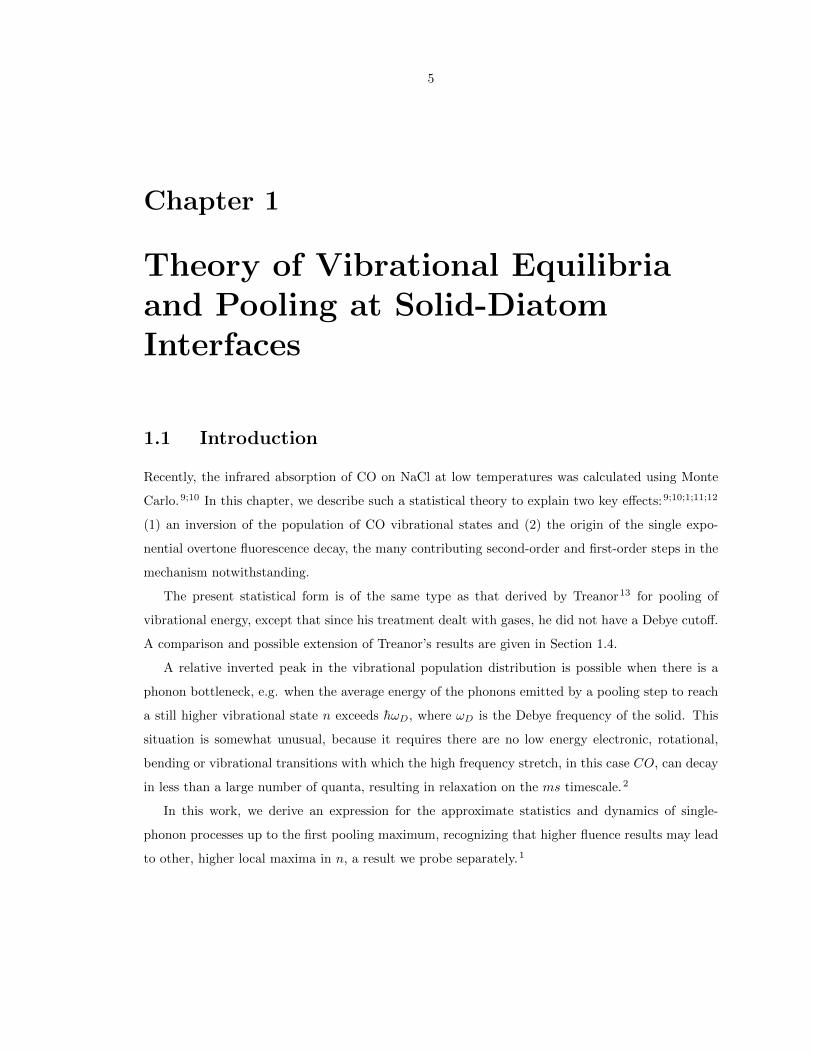
timescale (the reference1 gives further details of the calculation). The result is seen in Fig. 1.1 and

is evidence of the usefulness of the theory in the present chapter for the constrained distribution

of vibrational quanta among the quantum states of the oscillator. The distribution given by Eq.

1.4 is not exact. Nevertheless the results demonstrate that it is a useful description of the inverted

distribution with its cuto↵ at n=10.

The � appearing in Eq. 4 can be evaluated independently from the following:

N

M=

Pne�n�

✏

n

kT

Pe�n�

✏

n

kT

(1.8)

A simple way of obtaining � from the value of N/M is to evaluate the right hand side of this

function for varied �, and then find the � corresponding to the experimentally known N/M . Given

an absorption rate constant from lasing of kabs = 9.0 x 10�4, one expects a long term excitation of

N/M = (1 � exp(�kabs⌧))/2 = 0.18 for the lasing duration ⌧ .2 From this value for N/M , we find

� = 130, agreeing to every significant figure with the result derived from kinetic Monte Carlo Pn, as

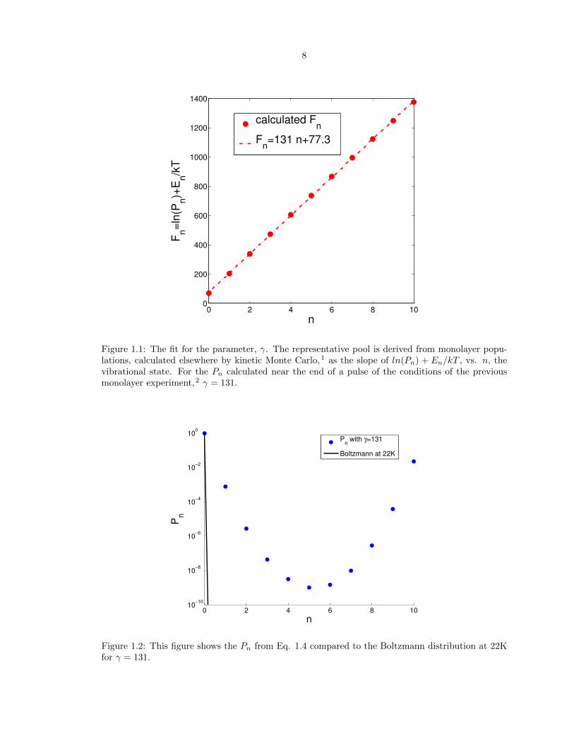
shown in Fig. 1.2.

1.3 Resulting Dynamics

The dynamics in the Monte Carlo Simulations are quite complex,10;9;1 in containing hundreds of

first-order and second-order reactions, but can be treated as having to an e↵ective single exponential

decay when there is a rapid equilibration process among the states n as follows. Consider the average

8

0 2 4 6 8 100

200

400

600

800

1000

1200

1400

n

Fn=

ln(P

n)+

En/k

T

calculated Fn

Fn=131 n+77.3

Figure 1.1: The fit for the parameter, �. The representative pool is derived from monolayer popu-lations, calculated elsewhere by kinetic Monte Carlo,1 as the slope of ln(Pn) + En/kT , vs. n, thevibrational state. For the Pn calculated near the end of a pulse of the conditions of the previousmonolayer experiment,2 � = 131.

0 2 4 6 8 1010

!10

10!8

10!6

10!4

10!2

100

n

Pn

Pn with !=131

Boltzmann at 22K

Figure 1.2: This figure shows the Pn from Eq. 1.4 compared to the Boltzmann distribution at 22Kfor � = 131.

9

number of quanta in any one site:

N =X

nmn (1.9)

In the loss of N vibrational quanta from the pooled surface, the non-radiative excitation of phonons

in the solid involves many phonons, and is slow relative to single-quantum pooling equilibration: the

latter involves only single excitations, whereas the former involves many such excitations simulta-

neously. The slow disappearance of quanta in the adsorbate is given by:

�dN

dt=

Xnmn (1.10)

If there is at each time t a rapid equilibration among the quanta in the adsorbate, then there

is a single exponential decay of N , N = N0e��t and mn = mn0e��t, so from Eq. 1.9 we have

dN/dt = ��P

nmn. We note that this temporal dependence of the mn, under rapid pooling

equilibration, leads to the same, single-exponential, temporal decay of all states equilibrated, with

time constant 1/�, in contrast to prior expectations for pooling on the H:Si(111) surface.4

Comparing with Eq. 1.10, we then have:

� =

PnmnPnmn

(1.11)

When applied to the present problem,1 this model with the theoretical constrained equilibrium

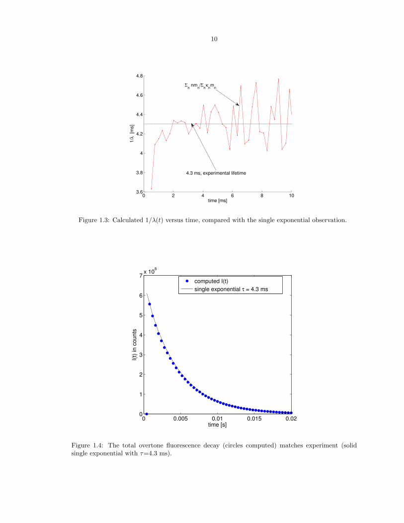
distribution given in Eq. 2.10 recovers a reasonably close time constant (3.6 ms for the present

theoretical result of Eq. 1.11 vs. 4.3 ms in the full Monte Carlo calculation and experimentally) and

single exponential behavior for each state in the pool with the same time constant. We can compare

the e↵ective single exponential decay rate with the actual computed results for the monolayer, as in

Fig. 1.3.

1.4 Discussion

The consequences of a novel regime of distribution of the vibrational quanta among the di↵erent

vibrational states are several-fold.14;13 We note the unifying simplicity of application of the model

for di↵erent surfaces and phases. While our CO:NaCl(100) simulations at several laser intensities

is a time-consuming calculation,1 the simplicity of the present approximate analytical distribution,

when valid, allows one to describe readily other results that may occur experimentally.

We note that the single exponential decay for individual states calculated in this work and else-

where9;10;1 indicates that a single exponential decay of individual states cannot be taken as evidence

against vibrational pooling, as has been suggested for the H:Si(111) surface.4 Single exponential de-

10

0 2 4 6 8 103.6

3.8

4

4.2

4.4

4.6

4.8

1/!

[m

s]

time [ms]

4.3 ms, experimental lifetime

"n nm

n/"

n#

nm

n

Figure 1.3: Calculated 1/�(t) versus time, compared with the single exponential observation.

0 0.005 0.01 0.015 0.020

1

2

3

4

5

6

7x 10

8

I(t)

in c

ounts

time [s]

computed I(t)

single exponential ! = 4.3 ms

Figure 1.4: The total overtone fluorescence decay (circles computed) matches experiment (solidsingle exponential with ⌧=4.3 ms).

11

cay, even of individual states as observed experimentally (see the discussion preceding Eq. 1.11),

does not rule out pooling of the vibrational excitation as long as the latter is rapid relative to the

decay to the solid, and this point plays a major role when considering fast bimolecular vibrational

processes such as single-quantum assisted non-resonant energy transfer. The key to a single expo-

nential is the validity of the approximation of rapid equilibration between the quantum states of

CO molecules on the surface. For example, if a particular state n0 has a relatively rapid decay rate

by energy loss to the solid (still slow relative to the pooling equilibration, but fast relative to all

other processes), the other n s rapidly refill the n0 population, so that all states n decay at the same

rate. In summary, rapid equilibration among the states relative to loss of quanta to the solid is

the key to understanding the single-exponential decay observed both in the experiment and in the

computations.

A comparison of the present derivation (CO on a solid) with Treanor’s13 (CO in a gas) is inter-

esting. The N -conservation step is crucial in both, and, up to our Debye-based cut-o↵, the resulting

distribution function is of the same form for both (Treanor’s Eq. 4.8 and our Eq. 2.10). In our case,

there is a restriction of domain of allowed n-states in the single-quantum exchange with the solid,

whereas in the gas phase the non-resonant transfer was aided by a smooth translational energy dis-

tribution. However, another di↵erence, purely technical, rather than physical, is in the minimization

of free energy in our derivation, as opposed to an entropy-maximization and a temperature ansatz

for � in Treanor’s. The latter ansatz requires further steps to be made rigorous, namely a calculation

of the energy E, entropy S, and an introduction of temperature, 1/T = dS/dE, to reach a rigorous

result, a result obtained simply by a free energy minimization as above.

Of particular interest in the present study is the inverted nature of the distribution, with a

maximum at some nmax = d!D/2!e�ee following a period of excitation. We note that this limit is

proportional to the Debye cuto↵ frequency and inversely proportional to the anharmonicity, so nmax

for CO:Si(100) would be 20 because !D=448 cm�1 for Si(100),15 assuming the same anharmonicity

for CO, while for H:Si(111) it would be 5, since 2!e�e = 90 cm�1 for that surface, assuming the

same !D as Si(100). Additional investigation of these surfaces using kinetic Monte Carlo and treat-

ing several experimental results4;16 is the topic of forthcoming work. Pooling equilibration, while

minimizing the free energy, also conserves the total number of quanta. Because of this constraint,

the population tends to lower its energy by occupying the highest vibrational states, and so inver-

sion is thermodynamically allowed, consistent with a constrained equilibrium statistical mechanics.

Complete decay, radiatively and non-radiatively, will occur to eventually yield a thermal equilibrium

population distribution, largely in the n = 0 state.

The present approximation is not restricted to phonon relaxation of high frequency vibrations on

solids, but is relevant in other situations that conserve N , the total number of vibrational quanta,

namely: situations where there is rapid single-quantum non-resonant vibrational transfer, faster

12

than dissipative processes. In all cases, there is then superimposed on these rapid exchanges the

slow decay of N . The theory may be extended to treat isolated molecules in matrix solids,17 and

multilayers of CO on NaCl(100).11;12

The validity of the equilibration approximation depends on the absorbed laser intensity. It

may be expected to be valid when the intensity is su�ciently high. The argument is as follows:

equilibration is valid when the decay rate for loss of quanta to the solid is small relative to the rates

of the pooling and depooling processes. Pooling is a second-order process and proportional to the

square of the light intensity. If the absorbed intensity is too low, the rate of realized pooling will be

too slow and the approximation fails.

Quantitatively, for monolayer CO:NaCl(100), where the observed fluorescence relaxation lifetime

is 4.3 ms, the calculated rate constant for the 1+ 9 to 0 + 10 pooling reaction is 5 x 107 s�1 from

the kinetic Monte Carlo calculations.1;10 For this case, wee see that the pooling rate constant, kpool

is 2 x 105 times faster than the rate of loss of single quanta to the solid, � ⇡ 1/(4.3ms) (noting

again slight variation around this mean lifetime over time as in Fig. 1.3). If kpoolP1P9 >> �P9, we

expect the equilibration condition to be satisfied when P1 >> �/(kpool) ⇡ 5 x 10�6. Knowing or

estimating the cross-section for the absorption and a lifetime for the loss, from n = 1 to n = 0, for

quanta to the solid, one can estimate what laser intensity is needed to obtain any P1.

In the case of possible vibrational pooling in H:Si(111) Sum Frequency Generation (SFG) pump-

probe experiments, there was observed single exponential decay of the n = 1 state.4 There was also

observed a hot band,16 whose observed lifetime is the same as that for recovery of the fundamental

at room temperature, 0.9 ns. If the rapid equilibration (fast-pooling) approximation holds, then all

0 < n nmax should have the same single-exponential rate of relaxation, identical to the rate of

n = 0 recovery. If there were no equilibration, the lifetimes for n = 1 and n = 2 would be quite

di↵erent. For example, computations18 for a Bloch-Redfield dynamics gave an intrinsic lifetime for

the n = 2 state of 0.13 ns, and for the n = 1 state, 0.9 ns. From previous calculations of the pooling

rate constant,19 the rate constant for the 1 + 1 to 0 + 2 pooling reaction can be as high as ⇡ 2 x

108 s�1 on H:Si(111) under some experimental conditions.4;16 Based on the trends in pooling rate

constants for CO:NaCl(100),1 we expect the pooling rate constant for the 1 + nmax�1 to 0 + nmax

pooling reaction, kSiHpool , to be 7 x 109 s�1. In this case, the calculated pooling rate constant is ⇡ 10

times the observed rate of loss of single quanta to the solid (�SiH ⇡1/0.9 ns =1 x 109 s�1), and

P1 >> 0.1 would meet the equilibrium condition.

One can also examine the spectrally integrated SFG intensity in the previous hot band pump-

probe experiment for evidence of pooling on H:Si(111).16 We calculate that, after pumping, the

spectrally integrated SFG intensity is approximately 1/3 the value before pumping (inferred from

Fig. 1 of the reference16). One possibility for this reduction in integrated signal is that pooling is

fast, and much of the excited population is at the pooling maximum (nmax=5 for H:Si(111)). In

13

the previous experiment, following the pump, the SFG probed the 1840-2125 cm�1 range.16 If one

extended the SFG probe range to 1600-2125 cm�1 following the same pump as before,16 then it may

be possible to see if the majority of the spectrally integrated SFG intensity after pumping occurs at

n = 5. If fast-pooling occurs, one expects to see the 5 ! 6 transition dominate the post-pumping

SFG, which is expected to be around 1630 cm�1. We plan to discuss these and other issues20 for

the H:Si(111) system further in a later publication.

1.5 Conclusions

In the present theory, a simple distribution is derived by a free energy minimization during vibrational-

quanta-conserving pooling equilibration on solids. In particular, the following experimentally testable

predictions are made:

1- Statistical behavior is expected in vibrational equilibria, subject to the constraint of a slowly

decaying number of quantaN(t) when the vibrational equilibration is fast relative to all radiative and

non-radiative processes. This behavior can be described by the temperature and Debye frequency of

the solid along with the anharmonicity and fundamental frequency of the high frequency vibration.

2- All vibrational populations on surfaces in this model are described by restricting quantum

state n to the domain [0, d!D/2!e�ee]. The vibrational pools are coupled by all resonances and

near-resonances consistent with the preservation of the number of quanta.

3- Temporal single-exponential decay cannot be taken as evidence against vibrational pooling

despite the bimolecular rate constant behavior of individual rates and the unimolecular dependence

of other steps. Indeed, single exponential decay is the expected result if pooling equilibration is

faster than all decay processes.

14

Chapter 2

On the Infrared Fluorescence ofMonolayer 13CO:NaCl(100)

2.1 Introduction

Carbon monoxide (CO) on an NaCl(100) surface has been used as a model system for surface

vibrational excitation since around 1990.21;22;11;12;2 Several low temperature experiments have been

conducted on monolayers and multilayers of 12CO and 13CO, observing overtone (n + 2 ! n)

infrared fluorescence from monolayer 13CO excitation between the 2nd and 16th vibrational state2

and multilayer 13CO excitation reaching the 30th vibrational state.11;12 In the monolayer case, these

states were inferred by application of a filter (4200 - 3400 cm�1 transmitted) to the total integrated

overtone emission, and in the multilayer case these states were observed directly by the collection of

dispersed fluorescence.

Ewing et al.2 suggested that the mechanism for this localization of vibrational energy may be the

energetically favored vibrational pooling reaction, where a pair of Morse-like oscillator neighbors non-

resonantly transfer a vibrational quantum in a step that is exothermic due to the anharmonicity. This

vibrational energy transfer can in principle occur with sites further removed than nearest-neighbors,

but as a first approximation we focus on nearest-neighbor and single vibrational quantum exchanges.

The present formulation builds on a model of pooling and depooling rate constants given by

Corcelli and Tully for this system and this surface.9;10 We also use the same Kinetic Monte Carlo

(KMC) algorithm to evaluate the vibrational population evolution.9;10 We extend their pioneering

work to larger grid sizes (10,000 sites instead of 256), higher vibrational states (n = 45 instead of

n = 15�20), and to higher fluence laser conditions, including stimulated emission. Additionally, we

test our previous theoretical prediction of the explicit form of the constrained vibrational population

distribution function.1 In it, the n- domain of a pool is restricted by the maximum energy that can

be dissipated by pooling exchanges exciting only single-phonons in the solid.

15

2.2 Vibrational Exchange for monolayer CO

In a resonant vibrational exchange, the vibrational energy of the pair of neighbors is conserved in the

energy transfer, whereas in a non-resonant exchange, some of the energy excites or removes phonons

from the solid. This non-resonant case provides both a ladder-climbing mechanism for vibrational

excitation and a ladder-descending pathway for vibrational relaxation of the energy di↵erence in

the transition. This pooling-depooling e↵ect is described for a vibrational state n in the following

equations:

|ni+ |miWp

n,m�! |n+ 1i+ |m� 1i (2.1)

|n+ 1i+ |m� 1iWd

n+1,m�1�! |ni+ |mi (2.2)

where the W pn,m are pooling rate constants for a site in state n receiving a single vibrational quantum

of energy from a neighboring CO site initially in state m, and the reverse reaction is described by a

depooling rate constant W dn+1,m�1 .

We treat the e↵ect of pooling on the time-evolution of Pn(t), the probability of a single site being

in the nth vibrational state at time t, where n is the specific vibrational level whose time-evolution

is being described. We have:1X

n=0

Pn = 1 (2.3)

noting that, in the present model, every site is occupied and thus is in some CO vibrational state,

n = 0 and upward. Adsorption and desorption of CO are not considered, since the experimentally

observed dissociation rate is slower than 10�4s�1 at 22 K,23 and so should not be observed on the

20 ms experimental timescale, being 6 orders of magnitude slower.2 All simulations are at 22 K, the

temperature of the experiments.2;11;12

We define (dPn/dt)pd as the net rate of pooling and depooling of state n with nearest neighbors.

The pooling and depooling terms are described in Eqs. 1 and 2 in terms of the e↵ect on a specific

vibrational state n:

dPn

dt pd=

X

m

(W pn�1,m)Pn�1,m +

X

m

(W dn+1,m)Pn+1,m

�X

m

(W pn,m)Pn,m �

X

m

(W dn,m)Pn,m (2.4)

where Pn,m denotes the joint probability that there is a site in a vibrational state n and that there

is an adjacent site having m quanta (such thatP

m Pn,m = 4Pn, since every site has 4 neighbors).

Adding relaxation steps to the above, by energy loss to the solid on which the CO is adsorbed, the

16

vibrational state probability evolution of a site on a CO surface is:

dPn

dt pdrf=

dPn

dt p�d� nPn + n+1Pn+1 (2.5)

where the n denote the relaxation rate constants for transfer of energy to multiphonons in the solid.

The formulae for the relevant rate constants are given in Chapter Appendix A. A comparison of the

resulting rate constants of pooling, depooling, and relaxation along with fluorescence and overtone

fluorescence is given for many n’s in Figs. 2.1 (a) and (b).

These equations are used for 1 < n < 45, with a closure introduced into the equation for n = 45

in Eq 2.4 by making transfer to P46 impossible (P46 = 0). The vibrational populations Pn(t) can

then be obtained by kinetic Monte Carlo integration24 of all possible rates, as discussed by Corcelli

and Tully10 and references cited therein, using site-to-site surface hopping methods for the energy

transfer.

To allow the intensity of incoming light to be treated explicitly, we added to the KMC code terms

containing the absorption coe�cient kabs,l, the Einstein coe�cient for each laser, to (dPn/dt)pdrf in

Eq. 2.5. We considered only single-photon excitations from n = 0 to the n = 1 state:

dP0

dt= �kabs,l(P0 � P1) +

dP0

dt pdrf(2.6)

dP1

dt= kabs,l(P0 � P1) +

dP1

dt pdrf(2.7)

where the (dPn/dt)pdrf are calculated as in Eq. (2.5) above, and kabs,Mono = I�/(h!) is calculated

to be 9 x 104s�1 for monolayer laser conditions, 25 µJ in 5 µs, � = 3 x 10�17cm2molecule�1.2

To examine populations under lasing by higher fluence sources, we also examined excitation by the

CLIO Free Electron Laser (FEL) by following a single averaged macropulse, kabs,CLIO = 5 x 107s�1,

from 20 mJ in 8 µs.25 We note that, for higher fluence lasers, one must include both stimulated

absorption and emission.

Given that the rate of overtone fluorescence is slower than the energy transfer from the n state

to multiple phonons in the solid, the total overtone fluorescence intensity at time t, I(t), is given by:

I(t) =Nsim

A

X

n

k�v=2f Pn(t) =

X

n

In(t) (2.8)

where In(t) = (Nsim/A)k�v=2f Pn(t) and there are Nsim = 104 sites per trajectory, representing a

surface area A = 1.57 x 10�11 cm2 as in Corcelli and Tully.9 Resonant di↵usion out of the illuminated

spot is not considered.

The total dispersed overtone fluorescence, S(!), is obtained by integration of the fluorescence

17

intensity over a time ⌧i, the overtone fluorescence lines summed over all wavelengths:

S(!) =45X

n=2

Ln

Z ⌧i

0In(t)dt (2.9)

with the integrals approximated trapezoidally given Pn(t) and t from the program output up to

integration time ⌧i. The times ⌧i are chosen to represent di↵erent length fluorescence collection

experiments. Ln is the line shape, approximated for each line as a normalized Gaussian with

FWHM 10 cm�1. This lineshape is preferred over the Lorentzian by a fit to the experimental

dispersed overtone fluorescence emission from multilayers of CO on NaCl(100), for each overtone

line, at the same temperature as the monolayer experiment.26;11 Snapshots of Eq. 2.9 are also given.

We study the 13CO monolayer rather than a 12CO system following the experimental work

of Ewing et al.2;11;12 and the simulation of Corcelli and Tully9;10. This isotope was chosen for the

experiments to enhance the overlap of its fundamental frequency with the 12CO gas laser emission.27

Following Corcelli and Tully,9;10 the relaxation rate constants (n) are found by introducing a

system-bath coupling scale parameter � which multiplies the Debye density of states as a rough

estimate of the strength of coupling between surface oscillators and bath, and fixed such that the

experimentally observed total overtone fluorescence lifetime (4.3 ms) is recovered under monolayer

conditions. We find a single exponential decay matching the experimental observations, as in Fig.

2.2, for � = 0.470, close to the value of Corcelli and Tully (�CT = 0.522), and similar relaxation

rates of 1 = 6.7s�1 compared to 5.7 s�1 in the previous simulation. We find di↵erent rates in

the present calculation primarily because we use the experimental decay of overtone fluorescence

to fix the calculated e↵ective decay rate of overtone fluorescence, whereas the previous simulation

appears to have matched the computed fundamental fluorescence decay to the experimental overtone

fluorescence results.9;10;2

2.3 Kinetic Monte Carlo Results

We first analyze the total overtone fluorescence in Fig. 2.2 which has been fit via the system-bath

coupling parameter �. The calculated vibrational populations at the end of each laser-on period and

1 ms thereafter are compared in Figs. 2.3 and 2.4, respectively. We confirm that for the monolayer,

the overtone fluorescence results primarily from n=8� 10, as previously calculated.9;10

We also confirm in the computations the theoretically predicted distribution function derived

in another work,1 as in Fig. 2.5. Shown is the deviation that is linear in n, a deviation from the

Boltzmann distribution across the one-phonon domain restricted regime, with slope � = 131. We

discuss this result further in the next section.

The signal calculated in Figs. 2.6 and 2.7 is given is in total photons cm�2. The signal in Fig.

18

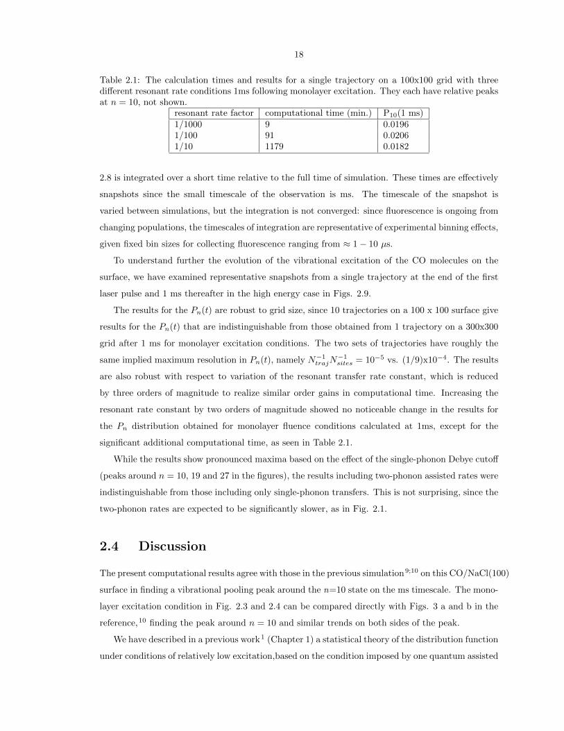
Table 2.1: The calculation times and results for a single trajectory on a 100x100 grid with threedi↵erent resonant rate conditions 1ms following monolayer excitation. They each have relative peaksat n = 10, not shown.

resonant rate factor computational time (min.) P10(1 ms)1/1000 9 0.01961/100 91 0.02061/10 1179 0.0182

2.8 is integrated over a short time relative to the full time of simulation. These times are e↵ectively

snapshots since the small timescale of the observation is ms. The timescale of the snapshot is

varied between simulations, but the integration is not converged: since fluorescence is ongoing from

changing populations, the timescales of integration are representative of experimental binning e↵ects,

given fixed bin sizes for collecting fluorescence ranging from ⇡ 1� 10 µs.

To understand further the evolution of the vibrational excitation of the CO molecules on the

surface, we have examined representative snapshots from a single trajectory at the end of the first

laser pulse and 1 ms thereafter in the high energy case in Figs. 2.9.

The results for the Pn(t) are robust to grid size, since 10 trajectories on a 100 x 100 surface give

results for the Pn(t) that are indistinguishable from those obtained from 1 trajectory on a 300x300

grid after 1 ms for monolayer excitation conditions. The two sets of trajectories have roughly the

same implied maximum resolution in Pn(t), namely N�1trajN

�1sites = 10�5 vs. (1/9)x10�4. The results

are also robust with respect to variation of the resonant transfer rate constant, which is reduced

by three orders of magnitude to realize similar order gains in computational time. Increasing the

resonant rate constant by two orders of magnitude showed no noticeable change in the results for

the Pn distribution obtained for monolayer fluence conditions calculated at 1ms, except for the

significant additional computational time, as seen in Table 2.1.

While the results show pronounced maxima based on the e↵ect of the single-phonon Debye cuto↵

(peaks around n = 10, 19 and 27 in the figures), the results including two-phonon assisted rates were

indistinguishable from those including only single-phonon transfers. This is not surprising, since the

two-phonon rates are expected to be significantly slower, as in Fig. 2.1.

2.4 Discussion

The present computational results agree with those in the previous simulation9;10 on this CO/NaCl(100)

surface in finding a vibrational pooling peak around the n=10 state on the ms timescale. The mono-

layer excitation condition in Fig. 2.3 and 2.4 can be compared directly with Figs. 3 a and b in the

reference,10 finding the peak around n = 10 and similar trends on both sides of the peak.

We have described in a previous work1 (Chapter 1) a statistical theory of the distribution function

under conditions of relatively low excitation,based on the condition imposed by one quantum assisted

19

emission in pooling, limited by the Debye frequency, h!D of the solid. The distribution function as

derived in the reference,1 is given by:

Pn(t) =mn(t)

M(t)=

e�(t)n�✏

n

kT

Pn e

�(t)n� ✏

n

kT

(2.10)

In this approximation, while in the domain of change of n by energy transfer accompanied by one-

phonon pooling, the Pn are primarily constrained in the interval [0, 10]. Clearly this constraint on

n does not hold for the CLIO excitation at short times, as in Fig. 2.3, but by 1 ms the assumption

appears to hold reasonably well for both lasing conditions, as in Fig. 2.4. As a result, we are able

to confirm in Fig. 2.5 that the constrained statistical theory described in the previous Chapter1

is in agreement with the presently calculated dependence on n. The systematic deviation from

the Boltzmann expectation with n is as theoretically expected in Eq. 2.10:1 � is the slope of

Fn = ln(Pn) + En/kT , vs. n, the vibrational state. If there is no component of the Free Energy

(Fn) which is dependent on n, then there should not be a dependence.

Using higher laser fluences than before and examining populations during the duration of lasing,

we have found substantial populations of many n > 16 states, as in in Fig. 2.3, including evidence

of strong inversion near the n = 22 state (3.5x1010photons cm�2 after 1 ms of collection, as in Fig.

2.7). By extending earlier work to higher intensities, these high lying states have been calculated

to exist in significant populations on this surface, and they result from the complex interplay of

rates, some of which are given in Fig. 2.1. Experimentally, levels as high as the n = 26 state

were inferred to have been observed in the dispersed fluorescence of multilayers of 13C18O.11 The

extent of the observability of higher states experimentally depends on the temporal resolution of the

apparatus. To our knowledge there have been no further experiments on the CO:NaCl(100) system

since 1990, and none with a higher fluence free electron laser source of the sort described here. These

calculations have spawned the related theory, and remain an important first step.

As seen in Figs. 2.6 and 2.7 after 1 ms following excitation, the distribution is more narrowly

peaked around an n = 10 maximum at lower fluences, and becomes broader and peaked around

slightly higher values at higher fluences. Over time, the evolution of pools by relaxation leads to a

characteristic dispersed fluorescence signature, calculated by Eq. 2.9.

For all the systems with high levels of excitation, as in Figs. 2.9, one notices immediately

a checkerboard pattern as a result of competition between di↵erent sites for the accumulation of

quanta. When excitation levels are somewhat lower, as in the snapshots 1 ms following excitation,

this competition is limited to single-phonon-assisted transfer rates, which are much faster than

multi-phonon-assisted transfer. This pattern is identified as an anti correlation between pooling

peak states (n > 1, but typically n = 8,9 or 10) or correlations between peaks and vacancies, and

it occurs within 2 microseconds after excitation, remaining anti correlated throughout all of our

20

simulations, as long as the pool states exist (four orders of magnitude in time). As a result, the

mean-field approximation of the master equation is not expected to give accurate results.

We include stimulated emission in these calculations for the first time. We suggest that the

previous experiments could not measure fluorescence (instead measuring the overtone) because of

the overwhelming stimulated emission signal during lasing. While arising from the much faster

stimulated emission process (kabs = 9 x 104 s�1), the photons collected would be indistinguishable

from fluorescence (k�v=1f = 11.4s�1). This e↵ect also adds many more Monte Carlo steps to the

calculation at the higher lasing fluence, more than doubling the computational time required.

It may appear at first unusual that, over time, the populations excited by higher intensity lasers

relax to similar distributions as those at lower fluence light, since three orders of magnitude of fluence

are spanned. This calculated result may be the signature of a constrained statistical behavior in a

physically based vibrational energy distribution, as explored theoretically in the previous chapter.1

2.5 Conclusions

In the present model, vibrational pooling leads to the accumulation of vibrational energy in 13CO

on NaCl(100). The model suggests substantial vibrational population inversion under existing laser

conditions.

Importantly, the calculation supports the constrained vibrational population distribution re-

cently derived theoretically for monolayers of high-frequency vibrations at solid surfaces where the

assumptions of the model hold.1 Further theoretical characterization of this high fluence regime,

where the previous theoretical assumptions fail, is the topic of ongoing research.

The following experimentally testable predictions are also made:

1- States as high as n = 32 may be excited with currently available laser conditions (1.5x104photons

cm�2 7-8 µs following lasing under CLIO FEL conditions), although the continued brightness of the

n ⇡ 10 pooled states through the ms timescale (4x1011 photons cm�2 after 8 ms as in Fig. 2.7 (b)

may restrict the observability of these higher states by dispersed fluorescence.

2- In addition to the inverted distribution with a peak at n = 10 persisting to 20 ms, there is

predicted to be a second inverted peak in the dispersed overtone fluorescence expected to appear

around n = 22, 2x109photons cm�2 after 1 ms of continuous collection, as in Fig. 2.7, when the

absorbed laser fluence prior to relaxation lifetime is increased to Free Electron Laser intensity.

21

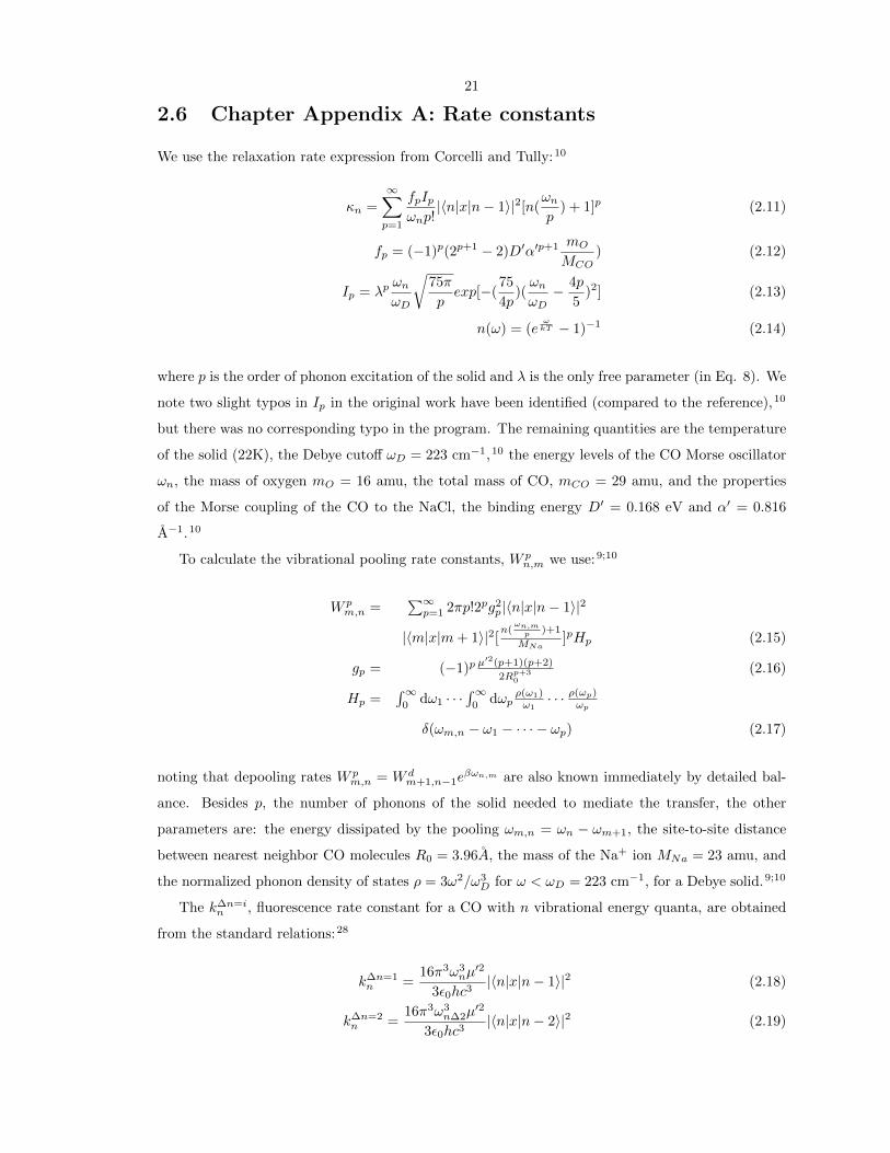
2.6 Chapter Appendix A: Rate constants

We use the relaxation rate expression from Corcelli and Tully:10

n =1X

p=1

fpIp!np!

|hn|x|n� 1i|2[n(!n

p) + 1]p (2.11)

fp = (�1)p(2p+1 � 2)D0↵0p+1 mO

MCO) (2.12)

Ip = �p !n

!D

r75⇡

pexp[�(

75

4p)(!n

!D� 4p

5)2] (2.13)

n(!) = (e!

kT � 1)�1 (2.14)

where p is the order of phonon excitation of the solid and � is the only free parameter (in Eq. 8). We

note two slight typos in Ip in the original work have been identified (compared to the reference),10

but there was no corresponding typo in the program. The remaining quantities are the temperature

of the solid (22K), the Debye cuto↵ !D = 223 cm�1,10 the energy levels of the CO Morse oscillator

!n, the mass of oxygen mO = 16 amu, the total mass of CO, mCO = 29 amu, and the properties

of the Morse coupling of the CO to the NaCl, the binding energy D0 = 0.168 eV and ↵0 = 0.816

A�1.10

To calculate the vibrational pooling rate constants, W pn,m we use:9;10

W pm,n =

P1p=1 2⇡p!2

pg2p|hn|x|n� 1i|2

|hm|x|m+ 1i|2[n(!

n,m

p

)+1

MNa

]pHp (2.15)

gp = (�1)p µ02(p+1)(p+2)

2Rp+30

(2.16)

Hp =R10 d!1 · · ·

R10 d!p

⇢(!1)!1

· · · ⇢(!p

)!

p

�(!m,n � !1 � · · ·� !p) (2.17)

noting that depooling rates W pm,n = W d

m+1,n�1e�!

n,m are also known immediately by detailed bal-

ance. Besides p, the number of phonons of the solid needed to mediate the transfer, the other

parameters are: the energy dissipated by the pooling !m,n = !n � !m+1, the site-to-site distance

between nearest neighbor CO molecules R0 = 3.96A, the mass of the Na+ ion MNa = 23 amu, and

the normalized phonon density of states ⇢ = 3!2/!3D for ! < !D = 223 cm�1, for a Debye solid.9;10

The k�n=in , fluorescence rate constant for a CO with n vibrational energy quanta, are obtained

from the standard relations:28

k�n=1n =

16⇡3!3nµ

02

3✏0hc3|hn|x|n� 1i|2 (2.18)

k�n=2n =

16⇡3!3n�2µ

02

3✏0hc3|hn|x|n� 2i|2 (2.19)

22

where !n�2 is the frequency of the n to n-2 overtone fluorescence, µ0 is the coe�cient in the

transition dipole moment, dµ(x)/dx|x=0 (1.8D/A in the case of 13CO),10 and the matrix elements

can be evaluated, for example in a Morse oscillator basis. Following Gallas,29 the Morse oscillator

matrix elements are given by:

hn|x|n� 1i = 1a(k�2n)

⇣n(k�2n�1)(k�2n+1)

(k�n)

⌘1/2(2.20)

hn|x|n� 2i =�1

2a(k � 2n+ 1)

⇣n(n�1)(k�2n�1)(k�2n+3)

(k�n+1)(k�n)

⌘1/2(2.21)

where the Morse constants are a=2.209 A�1 and D = 12.3 eV and k = !e/!e�e = 185, !e =2130

cm�1 is the fundamental frequency of the Morse oscillator and !e�e = 11.50 cm�1 is the anhar-

monicity (such that !2 = 2084 cm�1). The resulting overtone fluorescence rate constants range from

k�n=22 = 0.239 s�1 to k�n=2

44 = 60.2s�1. The fundamental fluorescence rate constants range from

k�n=11 = 11.6s�1 to k�n=1

26 = 135s�1.

2.7 Chapter Appendix B: Units

To connect with units traditionally used in chemical kinetics, we describe the population evolution

equations below, adapting (dPn/dt)pdrf in Eq. 2.5 to more familiar units. Let Mn be the number of

sites that have n quanta. We then have Pn = Mn/M . Let P (m|n) be the conditional probability, in

particular the probability that given a site with n quanta, there is an adjacent site with m quanta.

So in Eq. 2.5 we replace the Pn,m’s with PnP (m|n)’s. The Pn’s replace the normal concentrations

cn in kinetics,

dPn

dt pd=

X

m

(W pn�1,m)Pn�1P (m|n� 1)+

X

m

(W dn+1,m)P (m|n+ 1)Pn+1

�X

m

(W pn,m)P (m|n)Pn �

X

m

(W dn,m)P (m|n)Pn (2.22)

As a result, the units of the second-order rates are technically per conditional probability of an

m neighbor, given an n-site under consideration.

23

(a)

0 10 20 30 40

100

102

104

106

108

n

rate

con

stan

t [s−

1 ]

κn

kΔv=1n

kΔv=2n

(b)

0 5 10 15 20 25 30 35 40104

105

106

107

108

109

1010

n

rate

con

stan

t [s−

1 ]

Wn,20

Wn,10

Wn,1

Figure 2.1: Comparison of relevant rate constants: (a) first-order rate constants of relaxation (n),fluorescence (k�v=1

n ) and overtone fluorescence(k�v=2n ) (b) second-order rate constants of pooling

(W pn,m for m =1,10 and 20). The second order e↵ect of pooling to state n from an m = 1 state

which requires an additional phonon to transfer to n � 10, and so W p10,1 ⇡ 10�3W p

9,1. As secondorder rate constants, the pooling and depooling rate constants should be multiplied by a conditionalprobability if one wishes to compare with the first order rate constants, leading to units [s�1 perunit conditional probability P (m|n)], as discussed in Chapter Appendix B.

24

0 5 10 15 20 10 12 14 16 18 200

0.5

1

1.5

2.0

2.5

3.0

time [ms]

I(t) [

1014

pho

tons

s−1

cm−2

)

Figure 2.2: The total overtone fluorescence decay (circles computed) matches experiment (solidsingle exponential, I(t) = I(0)exp(�t/⌧), with time constant ⌧=4.3 ms).

5 10 15 20 25 30 350

0.05

0.1

n

P n

PCLIO(6 µs)

PML(6 µs)

Figure 2.3: The vibrational population 6 µs following beginning of pulse (near end of lasing).

25

2 4 6 8 10 12 14 16 18 200

0.02

0.04

0.06

0.08

0.1

0.12

0.14

0.16

n

P nPCLIO(1 ms)

PML(1 ms)

Figure 2.4: The vibrational population 1 ms following the beginning of lasing.

0 1 2 3 4 5 6 7 8 9 100

200

400

600

800

1000

1200

1400

n

F n=ln(

P n)+E n/k

T

calculated FnFn=131 n+77.3

Figure 2.5: The fit of the computed results to the theory-based expression permits the evaluation ofstatistical parameter � = 130, from the slope of the linear fit on the restricted n domain. A typicalresult for Pn after 4 ms following monolayer excitation is displayed, although this � is representativeof those where the restricted n-domain assumption holds.

26

(a)

3500 3600 3700 3800 3900 4000 41000

2

4

6

8

10

12

14

16

S(ω

) in

109 p

hoto

ns c

m−2

ω [cm−1]

10

11

9

(b)

3500 3600 3700 3800 3900 4000 41000

1

2

3

4

5

6

7 x 1010

S(ω

) in

1010

pho

tons

cm−2

ω [cm−1]

10

9

8

Figure 2.6: The theoretical dispersed fluorescence (assuming perfect collection e�ciency) for a mono-layer under the experimental monolayer lasing conditions (kabs=9 x 104s�1), integrated over a (a)1 ms and (b) 20 ms period after the beginning of lasing.2 The temporal integration was calculatedtrapezoidally from Pn(t) at 79 time points spread equally over the length of calculation.

27

(a)

3000 3100 3200 3300 3400 3500 3600 3700 3800 3900 4000 41000

1

2

3

4

5

6

ω [cm−1]

S(ω

) in

1010

pho

tons

cm−2

15

2022

10

(b)

3500 3600 3700 3800 3900 4000 41000

.5

1

1.5

2

2.5

3

3.5

4

4.5

5

S(ω

) in

1011

pho

tons

cm−2

ω [cm−1]

10

9

8

Figure 2.7: The theoretical dispersed fluorescence (assuming perfect collection e�ciency) after (a)1 ms and (b) 8 ms following CLIO excitation of a monolayer (averaged over a macro pulse for thehighest fluence currently available at that wavelength, kabs,CLIO = 5 x107s�1 for 8 µs, or 20 mJ).We note that, in (a), the appearance of a tiny higher n shoulder around n = 22 (which is even morepronounced as a relative peak at shorter times, not shown), but that the signal on the ms timescaleis overwhelmed by fluorescence from lower n and the distribution becomes the same as that for themonolayer under continued observation.

28

(a)

3650 3700 3750 3800 3850 3900 3950 40000

1

2

3

4

5

6

7

8

9

S(ω

) in

106 p

hoto

ns c

m−2

ω [cm−1]

9

10

11

(b)

3700 3750 3800 3850 3900 3950 4000 4050 41000

.2

.4

.6

.8

1

1.2

1.4

1.6

1.8

2

S(ω

) in

108 p

hoto

ns c

m−2

ω [cm−1]

10

9

8

Figure 2.8: Snapshots of the theoretical dispersed fluorescence for a monolayer under the experi-mental monolayer lasing conditions (kabs=9 x 104s�1). The snapshots given are (a) 1 µs between 77and 78 µs following beginning of excitation and (b) 12.7 µs period ending 1 ms after the beginningof lasing, representative of the di↵erence in results at di↵erent temporal resolutions of collection.

29

(a)

(b)

Figure 2.9: The vibrational population of the surface for a single trajectory at the conclusion of aCLIO FEL pulse (figure (a), 8 µs excitation) and 1 ms thereafter (figure (b), kabs,CLIO = 5 x107s�1

for 8 µs excitation for both). For (a), the legend is: n=0-black, 10-red, 20-orange, 25-yellow, 32-white, highest level. For (b) : n=0-black, 5-red, 10-yellow, 12-white, highest level.

30

Chapter 3

Vibrational Pools at Solid-DiatomInterfaces: Chemical Potential andEmergent Correlation

3.1 Introduction

In an earlier chapter, we treated a diatomic adsorbate on a solid in terms of a distribution function

at any time t, Pn(t), corresponding to an equilibration among pools of N vibrational quanta in the

adsorbate in various states n. The upper limit of n nmax in the one-quantum assisted exchanges

was determined by the constraint of the Debye frequency !D of the solid.

Our prior theory treats the case where the domain is restricted.1 This is expected to be the case

at moderate intensities: high enough that pooling is faster than relaxation, but not high enough

that n > nmax can form. Whereas the rate for the 1 + 9 to 0 +10 pooling reaction was 5 x 107

s�1, given that a 1 is adjacent to a 9, the rate of the 1+ 18 to 0 + 19 pooling reaction is 2 x 105

s�1, given that a 1 is next to an 18. From prior rate constant calculations 19/19=1 x 104 s�1.

Thus, one may expect two-phonon pooling (e.g. 1+18 to 0 + 19) to be fast on this surface relative

to relaxation when P1 > 0.05, and it is not surprising that the kinetic Monte Carlo exceeds the

one-phonon assisted limitation. Additionally, one expects quanta from higher pools to be mostly

relaxed by the ms timescale.

3.2 Formation of higher pools

The mechanism of forming the higher pools, n > 10, under high intensity lasing is complex. The

n = 1 initially form linearly, saturating quickly under FEL lasing and the n = 2 pools form as a

result of 1+1 pooling among existing pairs, and forming at rate W1,1P1, as can be seen in Fig. 3.1.

This result follows naturally from our prior discussion of second-order rate constants.3

31

0 10 20 30 40 50 60 70 800

0.05

0.1

0.15

0.2

0.25

0.3

0.35

0.4

0.45

0.5

time in ns

P n

kabst, kabs=9e4 s−1

P1

W1,1P1t, W1,1(0.5)=7.9e5 s−1 P2

Figure 3.1: This figure shows the formation of P2, noting P1,ss ⇡ 0.5

Additionally, we find that the n = 10 and n = 27 pools form linearly with time. Beyond this,

we observe no polynomial temporal pattern in the Pn buildup during lasing. This is consistent with

the description of these states as bottlenecks, as assumed for the n = 10 state in prior work.1

To understand pooling in more detail, we consider the allowed Pn distributions and � in the

following section, before deriving the chemical potential for the CO:NaCl(100) surface specifically.

3.3 Evaluation of Pn for several N and �

While the form of the distribution function in our prior work may be familiar to some from an earlier

derivation in the gas phase,13 we take the time now to review the general forms of Pn that can be

taken for various levels of N. We note that, by the definition of N, � satisfied the relationship:

N

M=

Pne�n�

✏

n

kT

Pe�n�

✏

n

kT

(3.1)

We have noted previously that this was the distribution function resulting from restriction of the

surface to a constant number of vibrational quanta.1 Varying � and finding N from Eq. 3.1 we can

elucidate this relationship, as in Fig. 3.2, choosing the appropriate � for the amount of vibrational

excitation. However, because small errors in this fit lead to exponential di↵erences in Pn, the overall

32

124 125 126 127 128 129 130 131 132 133 1340

1

2

3

4

5

6

7

8

9

10

γ

N

Figure 3.2: This figure shows N vs. � for the domain restricted theory.

fit to observed Pn may not be very good even when the deviation from the linear fit relative to

Boltzmann expectation, as in Fig. 1.1, is very small.

Other forms of the one-phonon restricted distribution function are possible, if other long-lived

N (and thus �) are observed experimentally. If � = 130 we have the inversion as before, as seen in

Fig. 3.3.

� = 125 and 140 are evaluated for Pn and compared with the Boltzmann distribution in Figs.

3.4 and 3.5. Complete inversion, as in � = 140 is unlikely with laser-initiated transfer, because of

stimulated emission. When � = 125, n > 2 populations are too small to amount to anything at

22K (⇡ 1014 sites within the laser spot). We mean only to stress that, in situations where there is

not relative vibrational inversion on the n domain, there still may be deviation from the Boltzmann

expectation.

3.4 Analysis of the Correlation Function vs. Distance of Sep-

aration

The appearance of a checkerboard in earlier heat maps on the CO:NaCl(100) monolayer surface

was indicative of a nearest-neighbor anti-correlation between pools, as we have previously noted.3

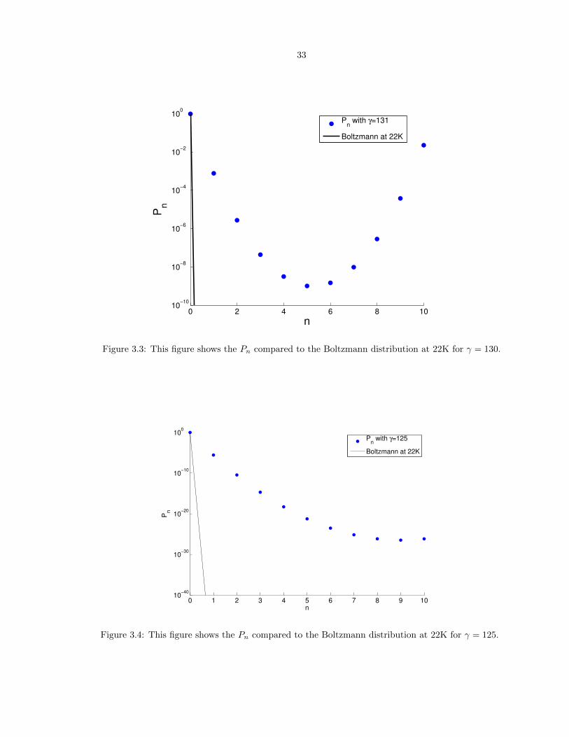
33

0 2 4 6 8 1010

!10

10!8

10!6

10!4

10!2

100

n

Pn

Pn with !=131

Boltzmann at 22K

Figure 3.3: This figure shows the Pn compared to the Boltzmann distribution at 22K for � = 130.

0 1 2 3 4 5 6 7 8 9 1010

!40

10!30

10!20

10!10

100

n

Pn

Pn with !=125

Boltzmann at 22K

Figure 3.4: This figure shows the Pn compared to the Boltzmann distribution at 22K for � = 125.

34

0 2 4 6 8 1010

!50

10!40

10!30

10!20

10!10

100

n

Pn

Pn with !=140

Boltzmann

Figure 3.5: This figure shows the Pn compared to the Boltzmann distribution at 22K for � = 140.

To examine whether this correlation extends further than nearest neighbor, we have calculated the

pairwise probability of neighbors of every distance on a 100x100 surface from a previous experiment.

Pairwise Probabilities of pools and pools (P10,10) and pools and vacancies (P10,0) vs. distance for

the two conditions is measured in Fig. 1. Because of the residual checkerboard e↵ect, pools are

slightly anti correlated with the vacancies of the next two neighbors, with still 10% anticorrelation

as far as 10 Angstroms from the pool (2.5 times the nearest neighbor distance of 3.96 Angstroms),

1ms following excitation by a free electron laser. At wide separations, the mean-field expectation

for Pn,m is recovered.

While this is only a two-dimensional calculation, presented in this chapter for the first time,

it may have implications for the behavior of the vibrational populations at surfaces in conditions

where relaxation is slow and the temperature is low, mean-field theory is not expected to hold for

the vibrational evolution master equation, such as for multilayers of CO on NaCl(100).12;11

3.5 Introduction of the Free Energy and Chemical Potential

We treat the equilibrated system at long times, consisting of the pool of n = 10, 9, 8 with an upper

cut-o↵ at n = 10, and consisting of another phase, this the pool centered at a higher n, with no

cuto↵ because of an alternative formation mechanism (e.g. under FEL lasing, as calculated before

by kinetic Monte Carlo).3 We proceed as we did previously,1 and minimize total free energy subject

to a given number of quanta. The result is the same as that obtained before, but now with no

35

5 10 15 20 25 300

0.02

0.04

0.06

0.08

0.1

0.12

0.14

0.16

distance from n to m (Angstrom)

Pn,m

P10,0

(R)

P10,10

(R)

Figure 3.6: The vibrational pairwise population 1 ms following the beginning of lasing, comparedwith the mean-field expectation of the pair considered, the dashed lines are guides for the eye:(black)- P10,0, the pairwise probability of a n = 10 state next to a n = 0 state (orange)-P10,10,the pairwise probability of a n = 10 state next to a n = 10 state (note complete anti-correlationof nearest neighbors). The mean field result for P10,0 and P10,10 are given by the horizontal lines.Note that, for neighbors, mean-field is a bad approximation, but for R >> R0, the nearest neighbordistance of 3.96 Angstroms, mean-field is recovered.

36

Debye-based constant constraining the pool to a restricted n domain. We have all pools using

equilibration.

When only n nmax pool is present, namely at lower fluences, the sum over n was only up to

n = nmax. We then have the free energy, F of a site, given that it is in a pool, given the Pn:

F =X

n>0

EnPn + kTX

n>0

PnlnPn (3.2)

where

Pn(t) =e�(t)n�

✏

n

kT

Pn e

�(t)n� ✏

n

kT

(3.3)

and we have avoided counting n=0 states because they are vacancies, not pooled vibrational quanta.

Thus, for the free energy of the pool given only N :

F = �NkT � kT ln(X

n>0

e�(t)n�✏

n

kT ) (3.4)

The remainder of this Chapter will focus on the confirmation of the derived form chemical potential

of the first vibrational pool of monolayer 13CO:NaCl(100), 0 < n 10, as given in Eq. 3.4, at both

high and low fluence lasing conditions and short and long times.

3.6 Results and Discussion

We are interested in finding the chemical potential of the new pooled surface. We then define the

chemical potential of the pool by a partial derivative with respect to the average number, and obtain

µpool = @F/@N = �kT .

If one plots the free energy and average number, with each a function of the underlying time,

as in Fig. 3.7 for an 8 ms CLIO trajectory, we find µpool=2120 cm�1. This is approximately �kT,

which was our prior domain-restricted fit under monolayer excitation conditions with 10�3 times

the fluence of the CLIO.1;3

We establish the N�kT behavior of the free energy further with several examples from our prior

work. For the monolayer, the results can be seen in Fig. 3.8 and for the 103 higher fluence condition

from the FEL source, the results are given in Fig. 3.9.

These figures confirm the fit of the derived form of the chemical potential derived in Eq. 3.4.

37

0 0.5 1 1.50

500

1000

1500

2000

2500

3000

3500

navg

F in

cm−1

y = 2120*x + 0.0662 F[Pn(t)]

linear

Figure 3.7: In this figure, we see F vs. N, and see the chemical potential (slope) is 2120 cm�1. From�kT in our prior work, we had estimated 1960 cm�1 based on � from the domain restricted theory.

0 0.005 0.01 0.015 0.020

100

200

300

400

500

600

700

800

time up to 30 ms

Fre

e E

ne

rgy

in c

m!

1

Calculated ! NkT (N from KMC)F[P

n], P

n from KMC

Figure 3.8: The fit of �NkT for 20 ms following Monolayer lasing.2;1;3

38

0 0.005 0.01 0.015 0.02 0.025 0.030

1000

2000

3000

4000

5000

6000

time up to 30 ms

Fre

e E

ne

rgy

in c

m!

1

Calculated ! NkT (N from KMC)F[P

n], P

n from KMC

Figure 3.9: The fit of �NkT for 30 ms following CLIO lasing.3

3.7 Conclusions

We conclude that the behavior of vibrational pools under intense excitation to higher vibrational

levels is usefully described by an addition to the previous theory: the description of pools in terms

of free energy per pool of �kTN , or the chemical potential of a vibration in a pool (µi = �kT ).

39

Chapter 4

On the Laser-Induced Desorptionof H2 from an H:Si(111) surface

4.1 Background and Introduction

Hydrogen surface chemistry has a rich history, and there was great interest in its behavior on

semiconductor surfaces such as silicon30;31;18;32;33;34;35;36 in the 1990s. This body of work includes

low-energy probes such as infrared (IR),33;31;37;30 Raman,34;38 sum frequency generation (SFG),4

thermal desorption,39;40 and theoretical calculations of the H:Si(111) surface.18

At that time, single exponential recovery of the ground state with time constant 0.9 ns was

observed.4 This single exponential behavior has been taken by the authors as evidence against

vibrational pooling on that timescale.4 We have shown previously1 that if pooling is the fastest rate,

one expects single exponential decay of every state with the same decay constant as the recovery of

the fundamental.

These SiH experiments4;33;31;37;30;34;38;39;40 have previously been interpreted in terms of non-

radiative (nr) deactivation by a multi-phonon excitation of the solid or possibly coupling to a bend.31

There are two additional known non-radiative processes that can also cause vibrational exchange and

are relevant for the present model: resonant vibrational exchange with nearby sites and non-resonant

vibrational energy transfer (pooling and depooling).9;10 These vibrational exchange mechanisms can

in principle occur with sites further than nearest-neighbors, but we restrict the discussion to nearest-

neighbors for simplicity.

Ma et. al.19 have studied the theory of resonant exchange and non-resonant vibrational pooling

and depooling in their three-state (n = 0, 1, 2) treatment of multiphoton absorption for this surface.

They concluded that “if the lifetime of the excited state is long enough, the oscillator has the

possibility to reach highly excited states through a series of pooling” steps. Previously, fluorescence

of highly excited CO on NaCl(100) arising from the excitation of the CO fundamental by an infrared

laser has been observed experimentally by Richardson and Ewing41 and has been interpreted by Tully

40

and Corcelli in terms of vibrational pooling on that surface.9;10 Our earlier work1;3 confirmed and

extended their model for CO:NaCl(100).

Depending on the incident light intensity, one might expect this e↵ect to be observed for the H:Si

surfaces as well, given the large mismatch between the Debye frequency of the solid (448 cm�1)10

and the fundamental SiH vibration (2087.3 cm�1) that requires many solid-state phonons to be

excited at once, leading to the qualitative expectation of a slow relaxation rate of the SiH state with

this mechanism.

In an earlier study,20 results were given to show that it is possible to desorb molecular Hydrogen

(a process that overcomes a bond of about 2.4 eV) using Free Electron Laser pulses in the infrared

(at 0.26 eV) with power 1 kW/macropulse at room temperature.20 It has since been indicated in

later work that the authors no longer had access to a FEL needed to repeat the experiment under

the same conditions. The original paper20 has since been corrected, e↵ectively retracted as not

reproduced. However, they no longer had access to a FEL, and the present theory leads to results

that are very sensitive to the intensity absorbed, so one may not expect the same results.

In the present chapter, we explicitly treat reactions between higher level vibrational states of

SiH, building on a recent three-state model of H:Si(111) of Ma et. al.19. We use a Morse potential

fixed to the first and second transitions of H:Si(111) to extrapolate rates of vibrational pooling

and depooling following the method of Corcelli and Tully. Otherwise, we use the same models for

relaxation and pooling as Ma et al. for ease of comparison.19 We explicitly treat laser overlap with

hot band states as well. This methodology extends the prior kinetic Monte Carlo work9;10;1;3 to the

H:Si(111) surface.

In order to compute the time-evolving vibrational probabilities for the states n on the surface, we

use the same prescription as before for the calculation of the pooling rates as given in the Chapter

Appendix. However, following previous experimental and theoretical work for this surface, we take

the relaxation rate dependence on n to be:,4;19

n = n1 (4.1)

with 1 the one free parameter in the model, the non-radiative decay rate of the n=1 state. While this

parameter is free, in that it is not set by ab initio calculation, it will be fixed by the experimentally

observed rate of decay,4 as was the case on CO:NaCl(100).1;3

For H2 desorption from the monolayer, the activation energy is 2.4 eV, or around 10 SiH vi-

brational quanta, as estimated by studies of thermally induced desorption.42 This concentration of

quanta in two nearest neighbors cannot be the case at low levels of excitation, because the cuto↵ sug-

gested by the domain restricted theory is the supremum of !D/(2!e�e) = 448/90, i.e. 5.1 Because

previous studies3 and the previous Chapter observed anti correlation between pools and excitation

41

in neighbors, one needs pooling beyond nmax for two neighbors to reach the desorption threshold.

This requirement suggests the use of a Free Electron Laser, which provides, on average, frequent

high fluence stimulation for 6-8 µs in ⇡ 104 micropulses, each some ps long and separated by fractions

of a nanosecond. It was stated in the retraction of the previous experiment,20 that the Vanderbilt

Free Electron Laser is a unique light source for this experiment.20 We note in passing that the Free

Electron Laser at the Centre Laser Infrarouge d’Orsay (CLIO) facility has an almost identical power

and pulse structure to that of the now defunct Vanderbilt source,25 and suits the selective desorption

experiment quite well. Our calculations of the FEL pulse could equally well describe either laser.

We can develop the theory further for the loss of H2 pressure experimentally.20 Let us assume

that the desorption of H2 occurs with e↵ective first order rate constant k0 for some concentration of

excited SiH vibrations ([SiH]). Allowing for a pump of rate constant k, we have the following first

order equation for the change in pH2 , the pressure of H2 remaining in the chamber:

dpH2

dt= k0[SiH]� kpH2 (4.2)

assuming a steady-state, k0[SiH] = kpH2 , and given the first order loss relation �d[SiH]/dt =

k0[SiH], we then have

�dpH2

dt= k0pH2 (4.3)

So that the apparent half-life of the yield in the chamber gives information on the reaction rate,

krxn, for instance, if we take take krxn ⇡ k0/(< P5 >)2. For the calculated value of P5 ⇡ 10�2

during lasing as in Fig. 4.2, the average value of P5 over the 1/30 s time interval between pulses

is < P5 >= P5 x 6/33, 333 = 2 x 10�6, assuming all states completely relax immediately when the

laser is not on. For a measured value of k0 ⇡ ln(2)/0.5 s�1, this implies a reaction rate constant of

⇡1 x 1012 s�1.

4.2 Results

The first calculations in this chapter follow the evolution of the vibrational populations on the surface

without allowing desorption, and fix the free parameter (the system-bath coupling, e↵ectively setting

n, the rate of decay to phonons). In these studies, we are able to determine if neighbors ever reach

higher levels of excitation, after first fixing all the parameters in our model with relaxation lifetimes

derived from apparent SFG decay time constant for the system.4 One can see the fit, done at 95K

in Fig. 1.

With the relaxation constant 1 fixed, we can then examine whether the conditions for a reaction

exist on the surface at any point under the SFG pump conditions 35 µJ in a 20 ps pulse. The time

42

0 0.2 0.4 0.6 0.8 1 1.2 1.4 1.6 1.8 2x 10−9

0

0.2

0.4

0.6

0.8

1

1.2

1.4

P 1(t)/P

1(0)

time, up to 2 ns

calculated at 95 K, 1/κ0= 5ns

τ = 1.4 ns

Figure 4.1: The fit to the experimental loss of P1,4 1 = 1/(5x10�9) s�1

evolution of the vibrational populations is given in Fig. 4.2.

CLIO excitation (at 1kW/macropulse, kabs = (I�)/(h!) = 2 x 109 s�1) leads to some neighbors

having combined vibrational energy of 10 quanta or greater (greater than the 2.4 eV activation en-

ergy). To examine desorption explicitly, we then extend the method to include an explicit description

of the process of associative desorption in the Monte Carlo algorithm; A four frame visual overview

of the evolution of the H2 molecules evolving from the lattice is given in Fig. 4.3 (a)-(d). For now,

in the calculations, we assume that the rate constant for associative desorption is around 1 x 1012

s�1, consistent with our estimate from the end of the first section in this chapter (1 x 1012 s�1) and

the order of magnitude of the fastest rates considered (resonant vibrational transfer), and simply

add this rate process in with all the others (pooling, depooling, and relaxation to phonons). The

actual rate of reaction may be faster: this reaction rate constant is 1/16 the first-order pre-factor

from thermal desorption calculations (6 x 1013 s�1).40

We also investigate the evolution of the desorption yield against fluence variation computationally,

now without any free parameters, to lay the groundwork for the proposed experiment. One can see

the dependence of the desorption yield of H2 on fluence in Fig. 4.4.

43

0 1 2 3 4 5 6 710−4

10−3

10−2

10−1

100

n

P n

Figure 4.2: The Pn vs. n 1.9 ns after lasing with prior conditions.4

4.3 Discussion

At short times, for instance in the 2 ns following the 20 ps pulse of the prior SFG pump,4;16 it

is impossible for any pair to have n = 10 or greater, because of the anticorrelation of pools,3.

Consistent pulsed excitation, pooling, and relaxation are required to reach a combined n = 10.

We note that the saturation behavior of pooling with intensity is at odds with the quadratic

behavior described in previously retracted experimental results,20 providing the present chapter

with further motivation in determining the H2 dependence on light Intensity.

Previous calculations including both inelastic phonon scattering and phonon emission assisted

vibrational pooling indicate that pooling by phonon emission may be expected to dominate when the

temperature is low.19 Thus, given the three temperatures we could choose to fix the final parameter

of our model, T = 95, 300 and 460 K from the prior SFG lifetime experiment,4 we choose the

lowest temperature, T=95K, and draw conclusions about desorption only at this low temperature.

Since the prior FEL was performed at room temperature, the comparison is indirect, and could be

improved at room temperature by the inclusion of inelastic phonon scattering rate constants.

In an analysis in our previous work,1 from previous calculations of the pooling rate constant,19

the rate constant for the 1 + 1 to 0 + 2 pooling reaction can be as high as ⇡ 2 x 108 s�1 on

H:Si(111) under some experimental conditions.4;16 Based on the trends in pooling rate constants

44

(a) (b)

(c) (d)

Figure 4.3: Snapshots of the evolution of H2 from a 50x50 surface under FEL excitation: (a) after100 ns (b)after 500 ns (c) after 1µs (d) halfway through lasing. We note that the colors indicateblack for n = 0 white for n = 21 in (b)-(d), with n = 21, outside the n = 1�20 domain, used to markthe sites that have evolved o↵ the surface by associative desorption (white). While we are unable torender the 111 surface (a hexagonal lattice), the square lattice connectivity in figures shown includesdiagonals up and to the right and down and to the left of each site, e↵ectively giving 6 neighbors ofequal distance. Thus we see diagonally desorbed molecules on the square lattice representation ofthe 111 surface.

45

0 0.5 1 1.5 2 2.5 3 3.5 4 4.5 50

0.1

0.2

0.3

0.4

0.5

0.6

0.7

0.8

After Single FEL Pulse with Power [kW/Macropulse]

P H2

Vanderbilt FEL Fluence

Figure 4.4: Yield of H2 after a single macropulse vs. Power of macropulse, assuming fast-pooling(calculations shown for µ0 = 1e).

46

for CO:NaCl(100),1 we expect the pooling rate constant for the 1 + nmax � 1 to 0 + nmax pooling

reaction, kSiHpool , to be 7 x 109 s�1. In this case, the calculated pooling rate constant is ⇡ 10 times

the observed rate of loss of single quanta to the solid (�SiH ⇡1/0.9 ns =1 x 109 s�1), and P1 >> 0.1

would meet the equilibration condition given in Chapter 1 as kpool1,9 P1 > �. However, we note that

the pooling rate constant leading to fast-pooling requires the incorporation of inelastic scattering by

phonons.19

As a first approximation, we take the transition dipole moment derivative from the previously

reported cross-section,43 finding a transition dipole of µ0exp =0.45 e,

p5 larger than that derived

from the derivative of the previous Density Funcional Theory calculations of the dipole moment, 0.2

e.19

The change of transition dipole from the prior calculation19 leads to an increase in the rate

constant by phonon emission from the previously calculated19 kpool1,1 = 4.2 x 106 to 6.2 x 107 s�1,

and kpool1,4 = 5 x 108 s�1. By the estimate developed in our prior work,1 this is a regime that is

not fast-pooling equilibrated, because kpool1,4 P1 < � =1 x 109 s�1 for all P1. For the moment, since

the transition rate constant goes with the 4th power of transition dipole (see Chapter 2 Appendix

A), we can modify this equation for unknown dipole moment to be µ0 = ↵µ0exp, allowing µ0 to vary

from the experimental value. The fast pooling test then becomes (5 x 108)P1↵4 < � =1 x 109 s�1,

which can be realized for ↵ > (4)1/4 = 1.414 (assuming P1 0.5). Especially given the recent

retraction by the same lab as the cross-section experiment, presented as a personal communication

in the literature,43 it would be preferable to have the IR absorption cross-section for the H:Si(111)

stretch determined in the literature independently. Regardless, we calculate the kinetic Monte Carlo

for the surface to see if desorption occurs by pooling including only phonon-emission, even outside

the fast-pooling regime.

One can also examine the spectrally integrated SFG intensity in the previous hot band pump-

probe experiment for evidence of pooling on H:Si(111).16 We calculate that, after pumping, the

spectrally integrated SFG intensity is approximately 1/3 the value before pumping (inferred from

Fig. 1 of the reference16). A possible interpretation for this reduction in the spectrally integrated

signal is that pooling is fast, and much of the excited population is at the pooling maximum (nmax=5

for H:Si(111)). In the previous experiment,16 following the pump, the SFG probed the 1840-2125

cm�1 range.16 If one extended the SFG probe range to 1600-2125 cm�1 following the same pump

as before,16 then it may be possible to see if the majority of the spectrally integrated SFG intensity

after pumping occurs at n = 5. If fast-pooling occurs, one expects to see the 5 ! 6 transition

dominate the post-pumping SFG, which is expected to be around 1630 cm�1.

Additionally, as in Figs. 4.3 (d) and 4.4, we note that the yield approaches an anti-percolation

threshold at high fluences. The physical maximum for number of sites desorbed is 1�1/(nneigh+1)

where nneigh is the number of neighbors for each site, because each site must have a neighbor

47

still on the surface with whom to react. This could explain one di↵erence between Temperature

Programmed Desorption (TPD) and Laser Induced Thermal Desorption (LITD) for the H:Si(111)

surface: LITD apparently leaves ⇡ 0.1 of the surface unreacted, compared with TPD.42 Such a

fractionally covered surface is measurable by either Atomic Force Microscopy or Second Harmonic

Generation44 following desorption.

4.4 Conclusions

In conclusion, in this chapter we present several results for H2 desorption from the H:Si(111) surface

that prompt the proposed re-evaluation experimentally and further research on the mixed isotope

surface. Despite not reaching the regime of fast-pooling for transfer by phonon-emission only, we

nonetheless recover the possibility of desorption without any free parameters in the kinetic Monte

Carlo. We note the following results, which may be tested experimentally:

1- The desorption of H2 from H:Si(111) is expected following excitation by a su�ciently intense

Free Electron Laser.

2- Saturation dependence of H2 yield with intensity per macropulse, as in Fig. 4.4, is observed,

as opposed to the I2 dependence reported in the retracted experimental reference.20

3- The final surface is expected to reach an anti-percolation threshold: not all Hydrogen will

evolve o↵ the surface by associative desorption, leaving a minimum of 14% for H:Si(111), and

1/(nneigh + 1) more generally for a vibration with nneigh neighbors.

48

Chapter 5

Self-shielding in theE1⇧(1)-X1⌃+

g (0) band of CO in ahot solar nebula

5.1 Introduction and Background

Calcium-Aluminum-rich Inclusions (CAIs) are some of the oldest condensates in our solar system,

estimated to be about 4.6 billion years old.45 Since their discovery,46 however, scientists have been

puzzled by the near unity slope of their three-isotope enrichment plot. Su�ce it to say that the

observed e↵ect in these plots is the enrichment of the rarer O isotopes (17O and 18O) with respect to

the original isotope when compared with levels elsewhere. A recent proposal put forth by Clayton,47

who made the initial discovery of the isotope e↵ect in CAI’s in 1973, suggests carbon monoxide

self-shielding at the X-point (hereafter X-pt.), may be responsible for this e↵ect. A substantial

portion of the astrophysics community,48;49 however, doubts this is a viable mechanism due to the

high temperatures (1000-1500 K) in the early solar system at this location, among other concerns.

Determining the validity of this model was a project for several of the first years of study, with a

longer term goal of elucidating the mechanism for oxygen isotope e↵ects in CAIs, a problem that

has now gone unsolved for 35 years.

Let us take a moment to examine Claytons hypothesis further. The absorption lines to the

same electronic states of CO and its isotopomers are at slightly di↵erent frequencies due to the

di↵erent masses of Oxygen isotopes. As C16O is much more abundant than C17O and C18O (2600:1

and 500:1 abundances respectively) regular CO will quench its frequency of light closer to the light

source than these isotopomers. As such, more of the rare isotopic CO is cleaved, on average, further

from the light source than the regular isotopomer, leading to a spatial separation of isotopes. If

CAIs then formed in a region of heavy atom isotopic excess, this could be an explanation for their

observed unusual isotopic distribution. Claytons proposal is that this spatial separation left a region

49

of isotopically enriched CO around 0.035 AU from the proto-sun at a temperature of between 1000

and 1500 K.

The predissociative state attained by a band 31 transition (X1⌃+g (0) to E1⇧(1)) is responsible

for 58% of C18O photodissociation in a translucent cloud model,50;51 and accounts for between 36

and 63% in other isotopomers (13CO and 13C18O). It dominates the dissociation and preferential

dissociation leads to isotope e↵ects, and it lies between 91-110 nm, a region that has little H2

absorption at low temperatures. As such, it is the natural starting point to test Claytons hypothesis,

and our calculations below take it as the only source of CXO isotopomer fractionation. We assume

throughout that the dissociation e↵ects of 13CXO on oxygen isotope ratios is small compared to

12CXO, since the 13CXO isotopomer accounts for only about 1% of the overall molecular abundance

in the nebula.

Claytons hypothesis is not alone in the attempt to explain the mass-independent isotope e↵ect in

CAIs. Another such theory, proposed by Lyons and Young,52 suggests CO self-shielding in a more

distant (and thus colder) region of the solar nebula. A second such theory, proposed by Marcus,53

involves isotope selective chemical reactions on the surface of CAI grains. This model assumes the

isotopic composition of the sun is like that of the Earth, which is inconsistent with more recent

measurements.54 Nonetheless, the proposed chemistry of that model remains a possibility.

A similar mass-independent isotope e↵ect has been observed in ozone both in the lab55 and

in the upper atmosphere.56;57;58;59;60 Initially a self-shielding of O2 mechanism was proposed,50;51

but that was quickly shown to be unlikely.61 Recent work62 indicates that RRKM theory, with a

non-RRKM symmetry-based modification, applied to the ozone formation reaction is su�cient to

explain the observed isotope e↵ect.

Here, we evaluate self-shielding at the X point, following Aikawa and Herbst,63 the equations

describing the temperature and number density of H2, in a minimum-mass solar nebula (MMSN)

are the following:

T (R) = 28(R

100)�0.5 (5.1)

n(R) = n0(R

100)�2.75exp(�d0(

1

R� 1

(R2 + Z2)�.5)) (5.2)

where n0 = 1.9 x 109 cm�3, d0 = GMsunµgas/(kT ) , and R is the distance from the Sun in units of

AU (1 AU = 1.5 x 1013 cm) along the midplane. Also, G = 6.67 x 10�8 dyne/cm2/g2 , Msun = 2

x 1033 grams, and µgas = 2.4 x mass of a H atom. Gas pressure is obtained from P = nkT. Note

that d0 is a function of R, as temperature also depends on R. Z is the height above the midplane of

the nebula, also in units of AU (see figure 1 for clarification). Our calculations are performed at the

50

Figure 5.1: A visual representation of the Aikawa-Herbst model. The colors indicate the numberdensities of molecular hydrogen (red-highest, yellow-medium high, green-medium low, blue- lowest).The arrows in the negative z-direction indicate the direction of incident intensity. The spirals atlarge R are representative of vertical mixing. Their amplitude indicates the strength of the mixing.Reproduced with permission.5

X-point (R=0.035 AU, Z=0), which results in high densities of all gases.

To better understand the model, consider Fig. 5.1. The region Clayton shielding will take place

is at the origin of the colored region. The origin is referred to as the X-pt. because the predominant

wind in this protonebular model is outward along the edges of the disk, and the X-pt. is then the

place where the top and bottom winds of the disk meet. One can see that the X-pt. is a region of

very high density, and, as discussed earlier, very high temperature. In our model, the predominant

light intensity comes from the Z direction i.e. from starts other than the sun. That area of low

density where the incident intensity originates is called the Inter-Stellar Medium or ISM. To modify

this near the X-pt. in our model, the intensity dependence is as if coming from the proto-star, but

we still take the incident intensity coming from along the Z axis.

Note that, in our model, the angle of incidence of incoming light is along the Z direction, but with

the intensity of the proto-sun. This makes our model di↵erent from Claytons (where incident light is

along the R direction) when we calculate shielding e↵ects in section III, and this approximation was

made because the computational machinery already exists for this model.52 As such, the present

conclusions are for our pseudo-Clayton hypothesis, where the light is incident from the top of the

nebula. Preliminary calculations for shielding with the correct geometry, incident light along the

R-axis, indicate little change.5

51

Table 5.1: Molecular Constants for the various isotopomers of CO in the X1Sg ground state. Allvalues given in cm�1. Note that e-parity is used for the P and R branches and f-parity is used forthe Q branch.

X1Sg 12C16O 12C17O 12C18OB0 1.92 1.87 1.83D0 6.1203 x 10�6 5.814 x 10�6 5.5300 x 10�6

H0 5.4794 x 10�12 5.074 x 10�12 4.733 x 10�12

Table 5.2: Molecular Constants for the various isotopomers of CO in the E1P excited state. Allvalues given in cm�1. Note that e-parity is used for the P and R branches and f-parity is used forthe Q branch.

E112C16O 12C17O 12C18O

v1 95082.93 95056.02 95031.9Be 1.94 1.89 1.85De 6.67 x 10�6 6.0 x 10�6 4.54 x 10�6

Bf 1.93 1.88 1.84Df 6.64 x 10�6 6.0 x 10�6 5.13 x 10�6

5.2 Computation of Absorption Spectra

The spectrum for the X1⌃+g (0) to E1⇧(1) transition has been determined with the high precision

of .003 cm�1 per resonance by Ubachs, et al.64 The importance of the high resolution spectrum

is that its correspondingly highly accurate molecular constants allow for reasonable extrapolation

to high temperatures, such as those found near the X point. Given this high resolution spectrum

and its correspondingly accurate molecular constants (see Tables 5.1 and 5.2), line positions in our

synthetic absorption spectra were calculate dusing the formula:

EE(J0)� EX(J 00) = vE +BEJ

0(J 0 + 1)�DE(J0(J 0 + 1))2 (5.3)

�BXJ 00(J 00 + 1) +DX(J 00(J 00 + 1))2

where J is the X1⌃+g (0) rotational state, J the E1⇧(1) rotational state, B the rotational constant,

and D the centrifugal distortion constant (given in Tables 5.1 and 5.2). We proceed to populate the

vibrational and rotational levels of the X1⌃+g (0) state thermally, recording the Boltzmann population

of each level. We consider the first 150 rotational levels (J) of the the ground vibrational state (v=0),

and their corresponding 150 rotational levels for the excited state (J with v=1). The population of

the X1⌃+g (0)(v=0,J=150) state is 1.359 x 10�17 at 1500K, indicating further rotational levels need

not be considered.

The computation of the absorption spectrum was carried out using a Voigt lineshape approxima-

tion for each line position (see Chapter Appendix for more detail). This approximation has shown to

be valid in many regimes,65 including the Gaussian and Lorentzian widths for which we use it here.

We take the natural Lorentz linewidth of all CO isotopomers to be 0.034 cm-1 (found in Ubachs for

52

Figure 5.2: A comparison of the Voigt, Lorentzian, and Gaussian lineshape for a single transition.

12C16O)64 and the Doppler width to have the usual temperature dependence (see Chapter Appendix

for more details). The Voigt profile, �v00,J 00,v0,J0 is normalized so thatR�v00,J00,v0,J 0dv = 1. The

Voigt profile has a Gaussian dependence near the center and a Lorentzian dependence in the line

wings, which is evident in Figure 5.2.

The peak intensity for a given v, J , J band is determined using the following formula :

�CXO(v, J00, J 0) =

X

J 00

N(J 00)�v00,J00,v0J 0 (5.4)

for a particular isotopomer CXO where N(J 00) is the normalized Boltzmann weight of that

rotational level, i.e.

N(J 00) =(2J 00 + 1)e�✓

r

J 00(J 00+1)/T

qrot(5.5)

where ✓r is the rotational temperature of CxO (equivalent to B0 for each isotopomer: 2.77 K, 2.70

K, and 2.64 K for C16O, C17O, and C18O respectively), J and T as defined previously, and qrot the

rotational partition function given by the 2nd order expansion:14

qrot =T

2✓R(1 +

✓r3T

+1

15(✓rT)2) (5.6)

�v00,J00,v0,J 0 is the cross-section for each rovibrational transition (v00, J 00 ! v0, J 0), satisfying the fol-

53

Table 5.3: Comparison of fv00,v0 for di↵erent isotopomers. All values from Eidelsberg.8

Isotopomer Band 3112C16O 2.4723 x 10�3

12C18O 2.4697 x 10�3

13C16O 2.4698 x 10�3

13C18O 2.4671 x 10�3

lowing relation:

�v00,J00,v0,J 0(!) =e2⇡

mecfv00,J 00,v0,J 0�(!) (5.7)

where �(!) is the normalized Voigt profile and fv00,J 00,v0,J 0 is the absorption oscillator strength.

The absorption oscillator strength is obtained from the band oscillator strength fv00,v0 using the

formula:8

fv00,J 00,v0,J0 = fv00,v0(!v00,J 00,v0,J 0

!0)(

SJ 00

2J 00 + 1) (5.8)

Where the is the position of the transition, !0 is the band origin (the position of the fictitious

transition v’,J’=0!v”,J”=0), SJ the Honl-London factor chosen appropriately for the band (P,Q,

or R) and the band oscillator strength fv00,v0 is obtained from Eidelsberg (2.4723 x 10�3 cm2).66 For

the X1⌃+g (0) to E1⇧(1) transition, the appropriate Honl-London factors are:66 SR

J 00 = (J 00 + 2)/4,

SQJ 00 = (2J 00 + 1)/4, SP

J 00 = (J 00 � 1)/4. The total �CO(�) profile was obtained by adding all

rotationally allowed transitions �CO(�, J 00, J 0).

We have made the approximation that the band oscillator strength is constant in all isotopomers

at 2.4723 x 10�3. This is a good approximation in the band under consideration, see Table 5.3.

This analysis was performed for each of the transitions from the ground vibrational and the

first two excited vibrational states of the X1⌃+g (0) to E1⇧(1) transition (with Honl-London factors

modified accordingly for each transition). The perturbation of this transition by the k3⇧(6) state has

been well characterized64 as well. While this interaction will perturb the resulting synthetic spectrum

and self-shielding calculations, as its rotational level dependence di↵ers between isotopomers, we

argue in the following section that its e↵ect is negated by the shielding by H2 in the nebula at

such high temperatures. The same argument goes for the plethora of other, as yet uncharacterized,

near-resonant excitations that will a↵ect this transition at such high temperatures.

The calculation of a complete CO spectrum is constrained by the lack of highly accurate values for

molecular constants of other electronic levels and other perturbative interactions. This accuracy is

absolutely crucial at temperatures as high as 1500 K, as highly excited rotational levels are populated

and small discrepancies in molecular constants or interactions begin to be magnified, resulting in

incorrect line positions for the higher J transitions have increased cross-sections due to the thermal

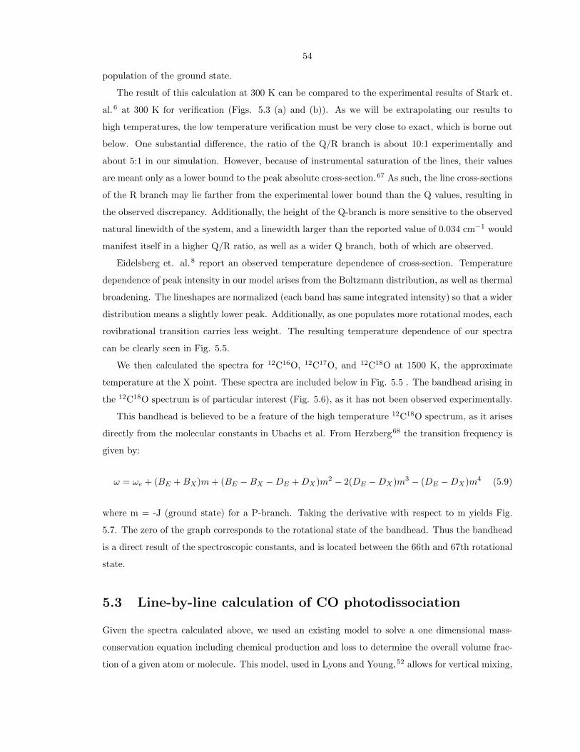
54

population of the ground state.

The result of this calculation at 300 K can be compared to the experimental results of Stark et.

al.6 at 300 K for verification (Figs. 5.3 (a) and (b)). As we will be extrapolating our results to

high temperatures, the low temperature verification must be very close to exact, which is borne out

below. One substantial di↵erence, the ratio of the Q/R branch is about 10:1 experimentally and

about 5:1 in our simulation. However, because of instrumental saturation of the lines, their values

are meant only as a lower bound to the peak absolute cross-section.67 As such, the line cross-sections

of the R branch may lie farther from the experimental lower bound than the Q values, resulting in

the observed discrepancy. Additionally, the height of the Q-branch is more sensitive to the observed

natural linewidth of the system, and a linewidth larger than the reported value of 0.034 cm�1 would

manifest itself in a higher Q/R ratio, as well as a wider Q branch, both of which are observed.

Eidelsberg et. al.8 report an observed temperature dependence of cross-section. Temperature

dependence of peak intensity in our model arises from the Boltzmann distribution, as well as thermal

broadening. The lineshapes are normalized (each band has same integrated intensity) so that a wider

distribution means a slightly lower peak. Additionally, as one populates more rotational modes, each

rovibrational transition carries less weight. The resulting temperature dependence of our spectra

can be clearly seen in Fig. 5.5.

We then calculated the spectra for 12C16O, 12C17O, and 12C18O at 1500 K, the approximate

temperature at the X point. These spectra are included below in Fig. 5.5 . The bandhead arising in

the 12C18O spectrum is of particular interest (Fig. 5.6), as it has not been observed experimentally.

This bandhead is believed to be a feature of the high temperature 12C18O spectrum, as it arises

directly from the molecular constants in Ubachs et al. From Herzberg68 the transition frequency is

given by:

! = !e + (BE +BX)m+ (BE �BX �DE +DX)m2 � 2(DE �DX)m3 � (DE �DX)m4 (5.9)

where m = -J (ground state) for a P-branch. Taking the derivative with respect to m yields Fig.

5.7. The zero of the graph corresponds to the rotational state of the bandhead. Thus the bandhead

is a direct result of the spectroscopic constants, and is located between the 66th and 67th rotational

state.

5.3 Line-by-line calculation of CO photodissociation

Given the spectra calculated above, we used an existing model to solve a one dimensional mass-

conservation equation including chemical production and loss to determine the overall volume frac-

tion of a given atom or molecule. This model, used in Lyons and Young,52 allows for vertical mixing,

55

(a)

(b)

Figure 5.3: (a) The synthetic 12C16O spectrum calculated at 300K. (b) Reproduced from Stark et.al.6

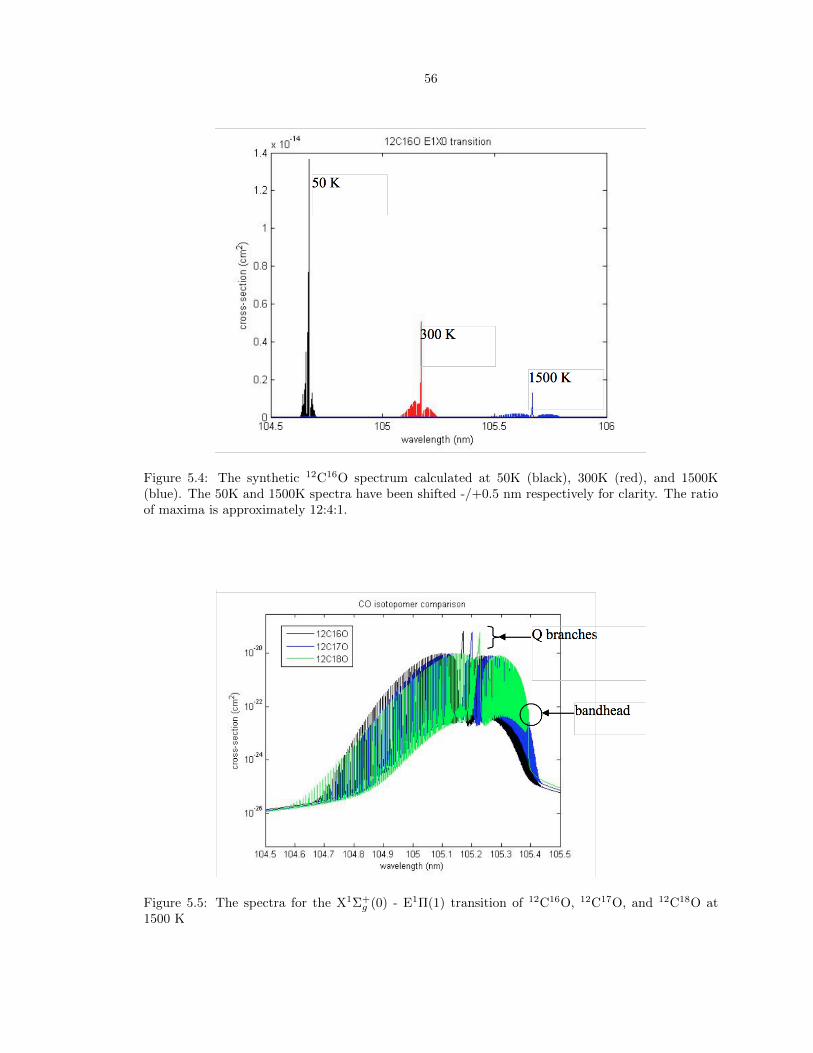
56

Figure 5.4: The synthetic 12C16O spectrum calculated at 50K (black), 300K (red), and 1500K(blue). The 50K and 1500K spectra have been shifted -/+0.5 nm respectively for clarity. The ratioof maxima is approximately 12:4:1.

Figure 5.5: The spectra for the X1⌃+g (0) - E1⇧(1) transition of 12C16O, 12C17O, and 12C18O at

1500 K

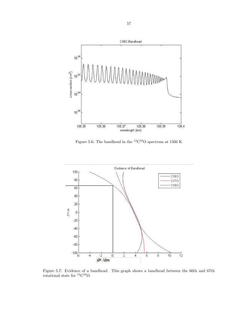
57

Figure 5.6: The bandhead in the 12C18O spectrum at 1500 K

Figure 5.7: Evidence of a bandhead. This graph shows a bandhead between the 66th and 67throtational state for 12C18O.

58

and is presently designed for radiation incident along the Z-axis (see Fig. 5.1).

CO is produced and destroyed by many di↵erent reactions in the model. For loss of CO by

photodissociation, Li for each CO isotopologue is given by:

LCXO = ✏e�⌧abs

(z)⇥H2(z)

Z

band31�CXO(�)�(�)F0(�)e

�⌧(�,z)d� (5.10)

where F0 is the modern day solar flux over band 31, ✏ is a flux enhancement factor relative to the

modern day sun (to account for the di↵erence in brightness of the protonebular sun, 1< ✏ <103), f

is the photodissociation quantum yield and is nearly unity for this band,50;51 ⇥H2(z) the shielding

function for H2,67 and ⌧(�, z) =P

i NCXO(z)�CXO(�) is the combined optical depth for the CO

isotopologues, NC16O, NC17O, and NC18O are the column densities of the respected isotopomers.

Dust opacity, ⌧dust, is identical for all isotopologues, and was parametrized in the same manner as

is done for the interstellar medium. As mentioned earlier, we take the incoming radiation along the

Z-direction in this model. As such, the column densities are obtained by integrating the Aikawa disk

model (Eq. 5.2) for number densities for fixed R (along the z-direction). The shielding integrals

describe the shielding e↵ects of the various CO isotopologues upon each other, and are the sole

source of non-mass dependent fractionation in our model. Using the shielding function for the H2

number density does not take into account the e↵ect of temperature on individual bands in H2, but

is a fit to the H2 absorption line wings at low temperature; a more detailed consideration of H2

temperature dependence will be found in the next section.

We assume all oxygen photodissociated from CO proceeds to H2O by the following reactions:

XO +H2k1�! XOH +H +H2

k2�! XOH2 +H

This is justified by calculating the k1 and k2 at 1500 K. Using experimental values and litera-

ture, closed-form temperature dependent approximations for k169 and k270 have previously been

found. Using these empirical formulae evaluated at the temperature (1500 K) and number density

(n(H2) 3.0x1018 cm�3) of the mid-plane of the X-point we obtain k1 ⇡2.49 x 10�12 cm3/s and k2 ⇡

6.803 x 10�12 cm3/s. These are bimolecular rate constants, and correspond to reaction time-scales

of 1.3 x 10�7s and 4.9 x 10�8 s respectively. This can be compared with another reaction which is

very fast at the X-point:

XO + CY Ok3�! CXO +Y O

This reaction would scramble any isotope e↵ect from shielding if the oxygen was not incorporated

into water in reactions 1 and 2 very quickly. A closed-form temperature dependent model for k3

has also been previously found.71 At the X-pt., we find bimolecular k3 1.00 x 10�11 cm3/s and a

timescale of 1.7 x 10�4 s. Thus, the incorporation of the isotope into water is 3-4 orders of magnitude

faster than isotope scrambling by exchange with CO at the X-point, and our assumption of rapid

incorporation of molecular oxygen into water appears justified.

59

Oxygen isotope composition for an unknown u was computed as:

�XOCOinitial

(u) = 103((XO)/16O)u/((XO)/16O)initial)� 1) (5.11)

for both O and CO in the nebula. Initial CO was assumed to have oxygen isotope ratios of 16O/18O

= 500 and 16O/17O = 2600. The shift in isotopic composition for an unknown u from a CO initial

reference to a standard mean ocean water (SMOW) reference is given by:

�XOSMOW (u) =�XOCOinitial

(u) (5.12)

+ �XOSMOW (COinitial) + 10�3�XOinitial(u)�XOSMOW (COinitial)

where x = 17 or 18, and �XOSMOW (COinitial) = �50%o. The oxygen isotope composition of total

nebular H2O is then given by:

�XOSMOW (H2Otot) =fH2Ocloud

�xOSMOW (H2Ocloud) + fH2Oss

(t)�xOSMOW (H2Oss)

fH2Ocloud

+ fH2Oss

(t)(5.13)

where the volume fraction of H2O from the parent cloud is fH2Ocloud

= 2 x 10�4 , the isotope

composition of the H2O in the cloud is = �50, fH2Oss

(t) is the volume fraction of H2O produced

from CO photodissociation (H2Oss) , and x = 17 or 18.

One can see in Fig. 5.8, referred to as a 3-isotope plot, that at the X-pt. and subject to

approximations elsewhere in this Chapter there is a self-shielding e↵ect similar to that observed in

CAIs (slope of 1) at 30 AU. Typically, materials found on Earth and in our solar system have a slope

of 0.52, and this is the anamolous e↵ect first discovered by Clayton.46 Deviations above a slope of

1 in the first quadrant of a 3-isotope plot are the result of regions where 18O is in isotopic excess

compared to 17O, when both are compared to levels found in SMOW. Deviations below indicate the

reverse e↵ect. We are constrained to the first quadrant (i.e. �17OSMOW , �18SMOW > 0) because the

self-shielding process postulated by Clayton results in an abundance of these heavy isotopomers,

which are then incorporated into solar nebular water.

5.4 Comparison with Navon and Wasserburg

Navon and Wasserburg61 carried out a similar calculation for the hypothesis of O2 self-shielding at

lower temperatures as an explanation of anomalous isotope ratios in CAIs. Their analysis di↵ered

from ours in that they approximated each rovibrational line as a product of step-up and step-down

functions added to a pseudocontinuum.

They concluded that O2 self-shielding was not a valid explanation because the 16O17O and

60

Figure 5.8: 3-isotope plot at 30 AU with temperature dependent CO cross sections. H2 absorptionby shielding function.7

16O18O spectra were enveloped by the 16O16O spectrum, even at the low temperatures in their

hypothesis (T = 300 K). This result was apparent despite their lineshape approximation because

the natural linewidth of O2 is much greater than CO, about a factor of 100 higher.61

For comparison with our spectroscopic results, consider the following. We have carried out

an identical analysis for the 12CO isotopomers 12C17O and 12C18O, modifying the linewidth by

the appropriate factor of 100 to see if our results agree with those of Navon and Wasserburg.61

The resulting spectra (overlaid in Fig. 5.9) show that the 12C17O and 12C18O are indeed completely

enveloped, resulting in no observed self-shielding. As a result, we have confidence both in the absence

of O2 self-shielding and of CO self- shielding at the X-point in the absence of other protonebular

considerations (see next section for discussion).

5.5 Absorption by H2

Di↵erential mutual shielding by H2 is accounted for by modifying Eq. 5.10 such that:

LCxO = ✏e�⌧dust

(z)

Z

band31�CxO(�)�(�)F0(�)e

�⌧(�,z)d� (5.14)

where now ⌧(�, z) =P

NCiO(z)�CiO(�) +NH2(z)�H2(�) , �H2 is the cross-section of molecular

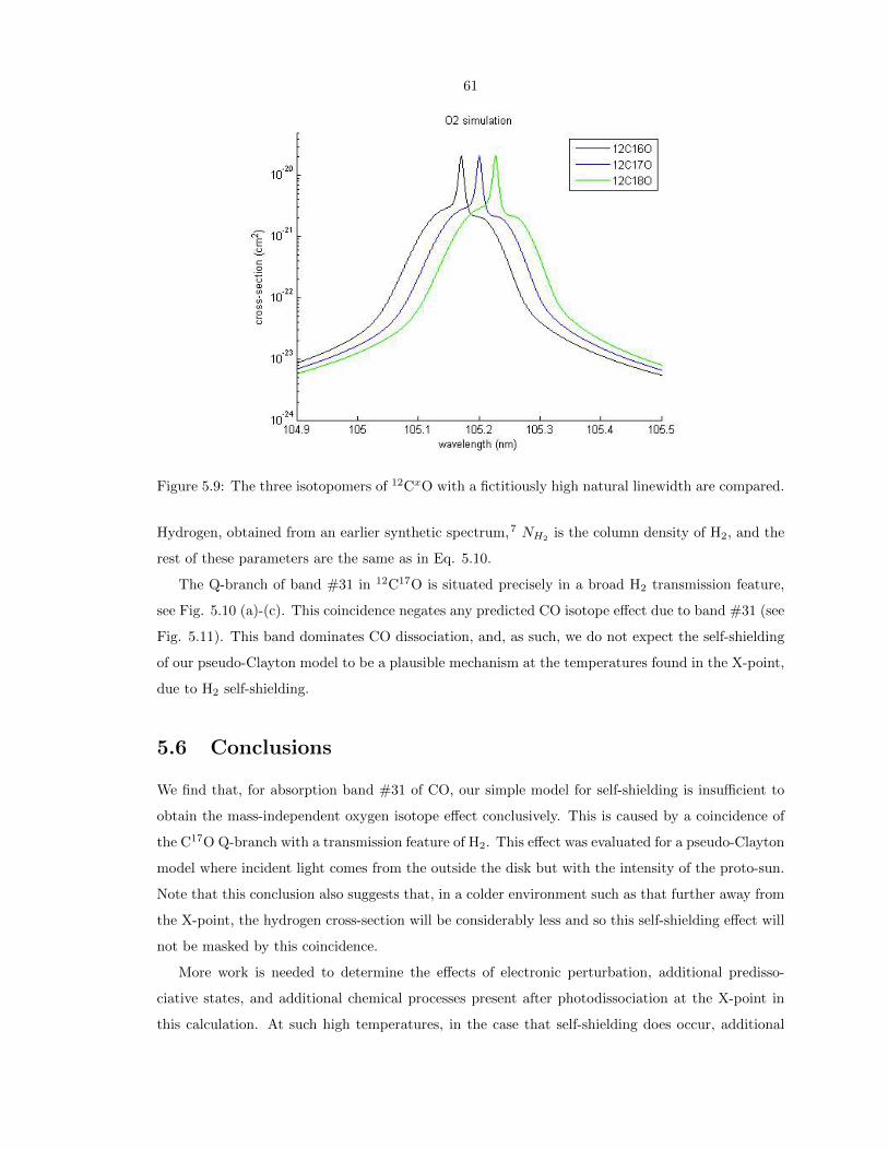
61

Figure 5.9: The three isotopomers of 12CxO with a fictitiously high natural linewidth are compared.

Hydrogen, obtained from an earlier synthetic spectrum,7 NH2 is the column density of H2, and the

rest of these parameters are the same as in Eq. 5.10.

The Q-branch of band #31 in 12C17O is situated precisely in a broad H2 transmission feature,

see Fig. 5.10 (a)-(c). This coincidence negates any predicted CO isotope e↵ect due to band #31 (see

Fig. 5.11). This band dominates CO dissociation, and, as such, we do not expect the self-shielding

of our pseudo-Clayton model to be a plausible mechanism at the temperatures found in the X-point,

due to H2 self-shielding.

5.6 Conclusions

We find that, for absorption band #31 of CO, our simple model for self-shielding is insu�cient to

obtain the mass-independent oxygen isotope e↵ect conclusively. This is caused by a coincidence of

the C17O Q-branch with a transmission feature of H2. This e↵ect was evaluated for a pseudo-Clayton

model where incident light comes from the outside the disk but with the intensity of the proto-sun.

Note that this conclusion also suggests that, in a colder environment such as that further away from

the X-point, the hydrogen cross-section will be considerably less and so this self-shielding e↵ect will

not be masked by this coincidence.

More work is needed to determine the e↵ects of electronic perturbation, additional predisso-

ciative states, and additional chemical processes present after photodissociation at the X-point in

this calculation. At such high temperatures, in the case that self-shielding does occur, additional

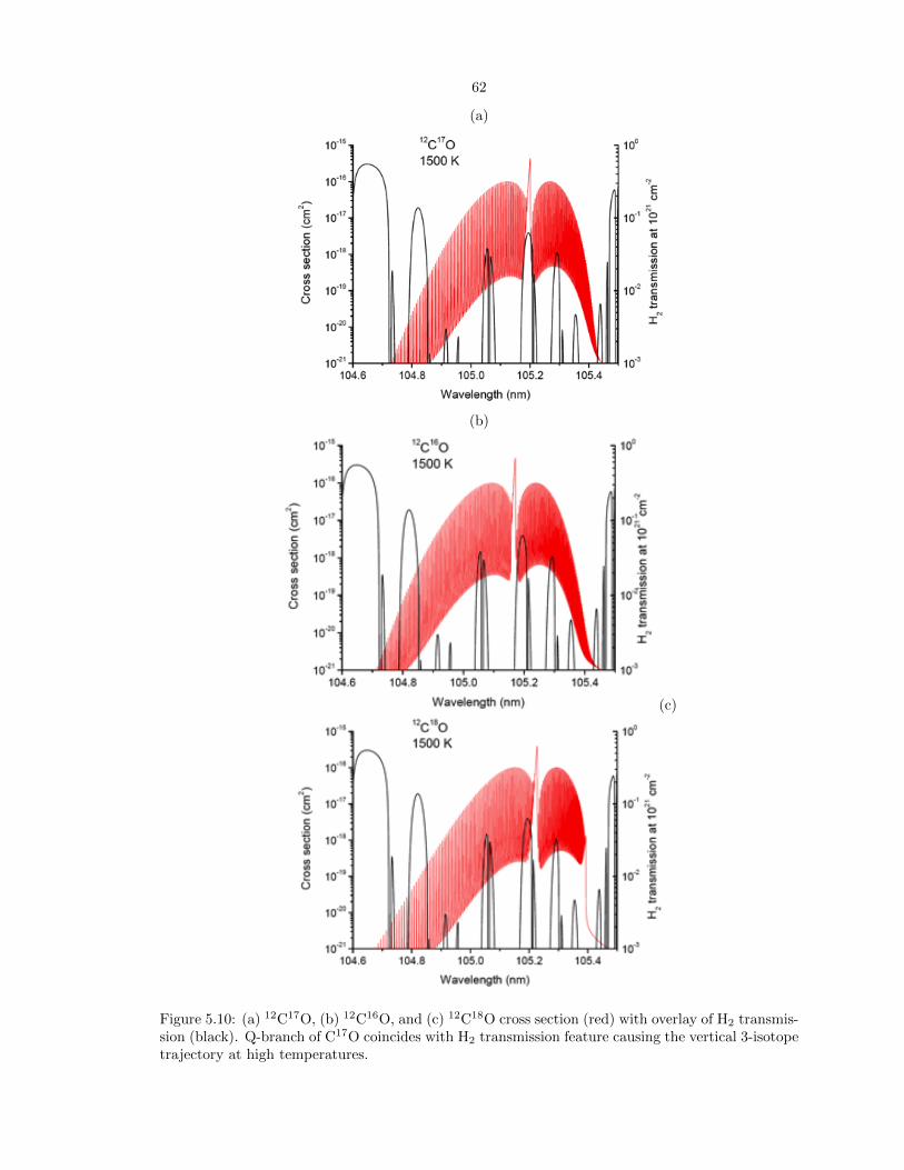
62

(a)

(b)

(c)

Figure 5.10: (a) 12C17O, (b) 12C16O, and (c) 12C18O cross section (red) with overlay of H2 transmis-sion (black). Q-branch of C17O coincides with H2 transmission feature causing the vertical 3-isotopetrajectory at high temperatures.

63

Figure 5.11: 3-isotope plot with H2 absorption cross sections at 0.035 AU, 0.87 AU, and 30 AU atthe mid-plane (Z=0).

reactions take place that could potentially skew the e↵ect further.

5.7 Chapter Appendix: Voigt Profile Approximation

The Voigt profile is a convolution of a Gaussian and Lorentzian lineshape, and has the general

formula:65

fv(v � v0) =

Z 1

�1fL(v

0 � v0)fD(v � v0)dv0 (5.15)

where fL(v0 � v0) and fD(v� v0) are the familiar Lorentzian and Doppler lineshapes respectively

and v0 is the line position. Including the specific forms these more well known lineshapes we arrive

at the following form of the Voigt profile:

fv(v � v0) =↵L

⇡3/2↵D

Z 1

�1

1

(v0 � v0)2 + ↵2L

exp(� (v � v0)2

↵2D

)dv0 (5.16)

where ↵L , and ↵D are the Lorentzian and Doppler widths. The Lorentzian width is assumed to

be the natural linewidth 0.034 cm�1. The Doppler width is given by ↵D = v0/c(2RT )1/2 where v0

is the central frequency of the rovibrationalline , c the speed of light, R the individual gas constant,

64

and T the temperature. We make the approximation of the Voigt profile as :

fv(v � v0) =(ln2

⇡)1/2

1

↵v(1� ⇠)exp(�⌘2ln2) +

⇠

⇡↵v(1 + ⌘2)(5.17)

� ⇠(1� ⇠)

⇡↵v(1.5

ln2+ 1 + ⇠)(0.66exp(�0.4⌘2)� 1

40� 5.5⌘2 + ⌘4) (5.18)

where ⇠ = ↵L/↵v , ⌘ = (v � v0)/↵v, and the Voigt half-width, ↵v, is given by

↵v = 0.5[↵L + (↵2L + 4↵2

Dln2)1/2] + 0.05↵(1� 2↵L

↵L + (↵2L + 4↵2

Dln2)1/2(5.19)

It is this closed form of the Voigt profile from the literature65 used in the present calculations.