GEOFIZIKA VOL. 32 2015

DOI: 10.15233/gfz.2015.32.9 Original scientific paper

UDC 556.313

Spatial analysis of groundwater electrical conductivity using ordinary kriging and artificial intelligence methods

(Case study: Tabriz plain, Iran)

Mehrdad Jeihouni1, Reza Delirhasannia2, Seyed Kazem Alavipanah1, Mahmoud Shahabi3 and Saeed Samadianfard2

1 University of Tehran, Faculty of Geography, Department of Remote Sensing and GIS, Tehran, Iran

2 University of Tabriz, Faculty of Agriculture, Department of Water Engineering, Tabriz, Iran3 University of Tabriz, Faculty of Agriculture, Department of Soil Science, Tabriz, Iran

Received 9 December 2014, in final form 3 September 2015

Artificial intelligence (AI) systems have opened a new horizon to analyze wa-ter engineering and environmental problems in recent decades. In this study per-formances of ordinary kriging (OK) as a linear geostatistical estimator and two intelligent methods including artificial neural networks (ANN) and adaptive neu-ro-fuzzy inference system (ANFIS) are investigated. For this purpose, geographi-cal coordinates of 120 observation wells that located in Tabriz plain, north-west of Iran, were defined as inputs and groundwater electrical conductivities (EC) were set as output of models. Eighty percent of data were randomly selected to train and develop mentioned models and twenty percent of data used for testing and validating. Finally, the outputs of models were compared with the corresponding measured values in observation wells. Results indicated that ANFIS model pro-vided the best accuracy among models with the root mean squared error (RMSE) value of 1.69 dS.m–1 and correlation coefficient (R) of 0.84. The RMSE values in ANN and OK were calculated 1.97 and 2.14 dS.m–1 and the R values were deter-mined 0.79 and 0.76, respectively. According to the results, the ANFIS method predicted EC precisely and can be advised for modeling groundwater salinity.

Keywords: artificial intelligence, ordinary kriging, electrical conductivity, Tabriz plain, groundwater

1. Introduction

Groundwater is the main resource for crops irrigation, drinking water and industry demands in the arid and semiarid regions. Irrigation with poor quality water can change the physical and chemical properties of the soils and conse-quently cause soil salinity and crops yield reduction (Ramsis et al., 1999).

192 M. JEIhOuNI ET AL.: SpATIAl ANAlySIS OF GROuNdwATER ElECTRICAl CONduCTIvITy ...

Although at the first glance it seems that environmental effects on groundwater are less than on the surface water, studies have proved that quantity and quality of groundwater are also affected by environmental factors as much as surface wa-ter resources (duNing et al., 2007). In some cases these effects are even more se-vere and permanent (Chandrasekharan et al., 2008). Another important issue in relation with these issues is the spatial variation of groundwater quality. Thus, groundwater quality cannot be assumed constant in the whole aquifer (Sun et al., 2009). determination of the groundwater salinity of an aquifer is a time-consum-ing and expensive process. Therefore the estimation of groundwater salinity is very important at unsampled locations. Recent advances in the non-classical methods have increased tendency to use spatial statistics or geostatistics for bet-ter understanding of spatial changes. Opposed to deterministic statistical meth-ods, the theoretical basis of geostatistics is assumes that the data and observa-tions are not random but spatially correlated (Chandrasekharan et al., 2008). Geostatistical analyses have a key role in sustainable management of groundwa-ter by identifying patterns and quantities at unsampled locations and providing estimated input parameters at regular grid points from random measurement lo-cations (Kumar, 2007). Also, the geostatistics is useful method for handling spa-tially distributed data, such as soil (Cemek et al., 2007; Gokalp et al., 2010) and groundwater contaminations (Arslan, 2012; Nas and Berktay, 2010). Kriging as one of the geostatistical methods is completely random linear model that is devel-oped based on probability theory. It includes different approaches: simple kriging, ordinary kriging, discjunctive kriging, universal kriging and indicator kriging.

The difference between kriging and other interpolation methods like inverse distance weighted (Idw) is that kriging uses the variance of the estimated val-ues (Buttner et al., 1998). Kriging has been broadly used in geology, hydrology, environmental monitoring, atmospheric sciences and pedology for interpolation of spatial data (McBratney et al., 1982; Stein, 1999; poon et al., 2000; Gringarten and deutsch, 2001; Jost and et al., 2005; Kholghi and hosseini, 2009; Oliver and webster, 2014; Jeihouni et al., 2015).

Based on yimit et al., (2011), kriging method has been used for mapping sa-linity of groundwater resources in China. In another research, Theodossiou and latinopoulos (2007) used kriging to estimate the level of groundwater in Anthemountas Basin of northern Greece. hooshmand et al., (2011) used kriging and co-kriging to estimate the absorption of sodium and chloride in groundwater of Bukan (north-west of Iran). despite of a high uncertainty in geostatistical models such as, ordinary kriging (OK) at unsampled locations, they are common methods for groundwater salinity mapping (hossain et al., 2007).

Soft computing (SC) is developing methodology, which aims to exploit toler-ance for vagueness, uncertainty, and partial truth to attain robustness, and traceability (Kabiri-Samania et al., 2011). Expert systems and artificial intelli-gence algorithms are relatively new subset of SC methods. Artificial neural

GEOFIZIKA, vOl. 32, NO. 2, 2015, 191–208 193

network (ANN) models are able to solve highly nonlinear problems (Khashei-Siuki and Sarbazi, 2013). In the last two decades the application of ANNs in the field of hydrology and water resources has been documented in many papers (Flood and Kartam, 1994; Gupta et al., 2000; Kazemi and hosseini, 2011; yesilnacar and Sahinkaya, 2012; pektaş and doğan, 2015).

ANNs are computational techniques based on theories of the massive inter-connection with neurons or nodes and parallel processing. They have been rec-ommended for solving scientific problems (Salas et al., 2000). ANNs can be used if available data are sufficient for modeling complex systems.

According to previous studies, ANNs are useful for assessing changes in groundwater level (lallahem et al., 2005). ANN performed very well in modeling the groundwater in Kaki City of India (Krishna et al., 2008). Chowdhury et al. (2010) applied OK and ANN methods for zoning of groundwater arsenic contami-nation and concluded that the neural network had better results than OK. yesilnacar et al. (2008) employed ANN to predict the nitrate concentration of groundwater in Turkey and showed that ANN has satisfactory results for model-ing groundwater nitrate.

Adaptive neuro-fuzzy inference systems (ANFIS) are noteworthy because they can learn the basic relations from numerical data, although the fuzzy rules can provide a clear linguistic description for the working of the model. Fuzzy sys-tems present the possibility of integrating logical information processing with the noteworthy mathematical properties of general function approximators (Setnes et al., 1998). The main advantage of fuzzy logic is representing its knowl-edge using simple IF-Then rules.

Many studies have discussed the hybrid technique by combining both ANN and fuzzy inference system (FIS) approaches due to ANNs non-linear structure and variables uncertainty in FIS model (Cheng and lee, 1999; hasebe and Nagayama, 2002; Kazemi and hosseini, 2011). Alvisi et al. (2006) predicted the water table by employing fuzzy logic and ANN methods.

Affandi and watanabe (2007) developed ANFIS and ANN based on the levenberg-Marquardt (lM) training algorithm to predict the daily fluctuation of groundwater level. They did not find significant differences between the two ap-proaches, and they concluded that soft computing algorithms can predict the groundwater daily level with high accuracy.

Tutmez et al. (2006) used ANFIS for modeling groundwater electrical con-ductivity (EC) from groundwater compositions. They showed that ANFIS with a few data has better capability to model EC than regression based conventional methods. Kholghi and hosseini (2009) compared both ANFIS and OK to esti-mate groundwater level and they found that ANFIS is more efficient than OK. Kazemi and hosseini (2011) studied OK, ANN and ANFIS for interpolating heavy metals in the Caspian Sea and they reported that ANFIS is the model with the lowest simulation error.

194 M. JEIhOuNI ET AL.: SpATIAl ANAlySIS OF GROuNdwATER ElECTRICAl CONduCTIvITy ...

In Iran, a large percent of irrigated fields is affected by the groundwater quality. The main goal of this study is to compare applications of different meth-ods including OK, the best linear unbiased estimator, ANN as a learning method that can be generalized to non-linear spatial model at unsampled locations, and ANFIS, as a combination of neural networks and fuzzy logic, for EC spatial estimation.

2. Materials and methods

2.1. Study area

Tabriz plain aquifer is located in north-west of Iran, with an approximate area of 2100 km2. This plain lies between latitude 37° 53´ to 38° 12´ N and longi-tude 45° 55´ to 46° 45´ E. The climate of the area is semi arid and average annual precipitation is 228 mm. Groundwater quality data of 120 observation wells in this aquifer (Fig. 1), which has been collected by the Ministry of Energy of Iran from 20th August to 18th September 2013, were used in the present research.

Figure 1. Study area and sample wells distribution.

2.2. Interpolation methods

This study focused on three specific spatial interpolation methods including OK, ANN and ANFIS. The longitude and latitude of wells defined inputs and EC set an output for each method. In all models 80% of the data set was used for model training, while 20% of data was used for testing and validating of the pre-dicted results. Brief explanations of each method are presented in following sections.

GEOFIZIKA, vOl. 32, NO. 2, 2015, 191–208 195

2.2.1. Ordinary kriging

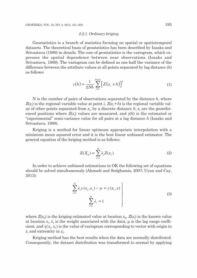
Geostatistics is a branch of statistics focusing on spatial or spatiotemporal datasets. The theoretical basis of geostatistics has been described by Isaaks and Srivastava (1989) in details. The core of geostatistics is the variogram, which ex-presses the spatial dependence between near observations (Isaaks and Srivastava, 1989). The variogram can be defined as one-half the variance of the difference between the attribute values at all points separated by lag distance (h) as follows:

γ hNh

Z x hii

N h

( )= +( )⎡⎣ ⎤⎦=

∑12

2

1

( )

(1)

N is the number of pairs of observations separated by the distance h, where Z(xi) is the regional variable value at point i, Z(xi

+ h) is the regional variable val-ue of other points separated from xi, by a discrete distance h; xi are the georefer-enced positions where Z(xi) values are measured, and γ(h) is the estimated or “experimental” semi-variance value for all pairs at a lag distance h (Isaaks and Srivastava, 1989).

Kriging is a method for linear optimum appropriate interpolation with a minimum mean squared error and it is the best linear unbiased estimator. The general equation of the kriging method is as follows:

Z X Z xi ii

N

( ) ( )01

==

∑λ (2)

In order to achieve unbiased estimations in OK the following set of equations should be solved simultaneously (Ahmadi and Sedghamiz, 2007; uyan and Cay, 2013):

λ γ μ γ

λ

i i j ii

N

ii

N

x x x x( , ) ( , )− =

=

⎫

⎬

⎪⎪

⎭

⎪⎪

=

=

∑

∑

1

1

1

λ γ μ γ

λ

i i j ii

N

ii

N

x x x x( , ) ( , )− =

=

⎫

⎬

⎪⎪

⎭

⎪⎪

=

=

∑

∑

1

1

1

(3)

where Z(x0) is the kriging estimated value at location x0, Z(xi) is the known value at location xi, λi is the weight associated with the data, μ is the lag range coeffi-cient, and γ( xi, xj ) is the value of variogram corresponding to vector with origin in xi and extremity in xj.

Kriging method has the best results when the data are normally distributed. Consequently, the dataset distribution was transformed to normal by applying

196 M. JEIhOuNI ET AL.: SpATIAl ANAlySIS OF GROuNdwATER ElECTRICAl CONduCTIvITy ...

lognormal transformation. Histograms of the training dataset before and after applying the lognormal transformation are shown in Fig. 2. Semivariogram mod-els were tested by geostatistical analyst in ArcGIS software to find the best fitted model to dataset.

а)

b)

Figure 2. The histograms of training dataset a) before lognormal transformation, b) after lognormal transformation.

GEOFIZIKA, vOl. 32, NO. 2, 2015, 191–208 197

2.2.2. Artificial neural networks

The ANN is designed based on a simulation of the human brain. It is made of simple processing units referred to as neurons. ANN is based on theories of the massive interconnection with neurons and parallel processes, where model can learn and accept an input and present related output. By providing sufficient training data, ANNs can achieve a high degree of accuracy and learn most com-plex relationships between input and output data. ANN is able to learn and gen-eralize from experimental data although they are noisy, defective or have non-linear pattern. unlike linear models, ANNs do not apply any limitations on statistical characteristics in the modeling process.

ANNs are useful in the cases where there is no idea about the complexity and structure of input and output data. Among ANN models, the ANN with back propagation (Bp) training algorithm (a multi-layer feedforward network trained according to error back propagation algorithm) is one of the most widely applied neural network model (li et al., 2012). The aim of this algorithm is to decrease total error (Chen et al., 2006).

In this study, an ANN with Multi-layer perceptron (Mlp) including four layers was used (Fig. 3). Network model trained by momentum optimization al-gorithm and TanhAxon as transfer function were selected. This structure was selected based on trial and error. Two hidden layers were used to adjust the neu-rons weights to achieve the desired output. For network model, longitude and latitude as the input and EC as the output were defined.

Figure 3. The structure of ANN used in this study.

2.2.3. Adaptive neuro-fuzzy inference system

ANFIS, introduced by Jang (1993), is an enhanced tool and data-driven mod-eling technique for specifying the behavior of vaguely defined complex dynamical systems (Kisi, 2005; dastorani et al., 2010). The structure of adaptive network is based on fuzzy If-Then rules, fuzzy inference and neural networks (Cheng and

198 M. JEIhOuNI ET AL.: SpATIAl ANAlySIS OF GROuNdwATER ElECTRICAl CONduCTIvITy ...

lee, 1999). ANFIS is a powerful universal approximation tool for vague and fuzzy systems (lee 2000). The fundamental structure of a FIS consists of five functional blocks and two conceptual parts including a FIS that make three parts (a rule base, a database, a reasoning mechanism). These blocks are shown sche-matically in Fig. 4., and an adaptive network has a multilayer feed forward net-work structure (Nayak et al., 2004).

Figure 4. Fuzzy interface system (Jang, 1993).

For the simplicity, it is assumed that the FIS under consideration has two inputs (x and y), longitude and latitude, and one output (Z) is EC. The architec-ture of ANFIS consists of five layers (Fig. 5), and the functions corresponding to nodes of the same layer are similar. Each input has two rules (A1 and A2, B1 and B2) in the first layer (input nodes), which can generate two rules in the second layer (rule nodes). A brief sketch of the operations of the five layers is given in the following (Jang, 1993):

Figure 5. ANFIS architecture.

GEOFIZIKA, vOl. 32, NO. 2, 2015, 191–208 199

Layer 1: input nodesEvery node i in this layer is used to perform a membership function:

O A xi i1 = μ ( ) for i = 1, 2 (4)

μA x

x ca

i

i

i

bi( )=

+−⎛

⎝⎜

⎞

⎠⎟

⎡

⎣⎢⎢

⎤

⎦⎥⎥

1

12 (5)

where x is the input to node i, and Ai are linguistic labels characterized by appro-priate membership function mAi; {ai, bi, ci} is the parameter set.

Layer 2: rule nodesIn this layer, every node is a circle node labeled Π which multiplies the in-

coming signals and sends the product out (6):

w A x B yi i i= ×μ μ( ) ( ), i = 1, 2 (6)

Layer 3: average nodes The i-th node’s output in this layer is the ratio of the i-th node’s output from

the previous layer to the total

ww

w wii=+1 2

, i = 1, 2 (7)

Layer 4: consequent nodesIn this layer, the first-order Sugeno fuzzy model is considered as a fuzzy in-

ference system:

O w f w p x q y ri i i i i i i4 = = + +( ) (8)

where {pi, qi, ri} is the parameter set in the consequent part of the first-order Sugeno fuzzy model.

Layer 5: output nodesA single node computes the overall output by summing all incoming signals.

Consequently, the defuzzification process transforms each rule’s fuzzy results into a crisp output in this layer (9).

200 M. JEIhOuNI ET AL.: SpATIAl ANAlySIS OF GROuNdwATER ElECTRICAl CONduCTIvITy ...

O w fw f

wi i ii

i ii

ii

5 = =∑∑∑

(9)

The network training was based on supervised learning. The aim was to train adaptive networks to be able to approximate unknown functions given by training data set and then find exact values of the parameters. unique charac-teristics of ANFIS are its hybrid-learning algorithm, the gradient descent meth-od and the least-squares method, to optimize the function parameters. In this study the trapezoid-shaped membership function (trapmf) with membership function (MF) numbers of [5 4] were used using hybrid optimal model. The MF type and number of MFs were selected based on trial and error. The result shows that trapmf with MF numbers of [5 4] type provides precise outputs and is opti-mum. Therefore, this mf was selected for modeling.

2.3. Model evaluation

Several parameters can be considered for the evaluation of groundwater EC estimations. In this investigation for evaluating the studied models, correlation coefficients (R) and root mean squared error (RMSE) were used as statistical criteria.

lower values of RMSE correspond to satisfying fit between data. If the main purpose of the model is prediction, RMSE is the best criterion for evaluating the accuracy of predicted values. The equations 10 and 11 were used to calculate the RMSE (Alsamamra, 2009) and correlation coefficients:

RMSEn

z zpi

n

= −=

∑1 02

1

( ) (10)

Rz z

z z

n

zz

n

p

pi

n

i

n

i

n

p

pi

n

i

n

=

−

−

⎛

⎝⎜⎜

⎞

⎠⎟⎟

⎛

⎝

⎜⎜⎜

= =

=

=

=

∑ ∑∑

∑∑

01

01

1

2 1

2

1⎜⎜⎜⎜

⎞

⎠

⎟⎟⎟⎟⎟⎟

−

⎛

⎝⎜⎜

⎞

⎠⎟⎟

⎛

⎝

⎜⎜⎜⎜⎜⎜

⎞

⎠

⎟⎟⎟⎟⎟⎟

=

=

∑∑z

z

ni

n

i

n

02

01

2

1

(11)

where zp are predicted and z0 are observed data and n is the number of observations.

GEOFIZIKA, vOl. 32, NO. 2, 2015, 191–208 201

3. Results and discussion

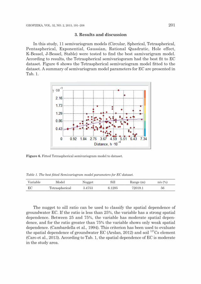
In this study, 11 semivariogram models (Circular, Spherical, Tetraspherical, Pentaspherical, Exponential, Gaussian, Rational Quadratic, Hole effect, K-Bessel, J-Bessel, Stable) were tested to find the best samivarigram model. According to results, the Tetraspherical semivariogoram had the best fit to EC dataset. Figure 6 shows the Tetraspherical semivariogram model fitted to the dataset. A summary of semivariogram model parameters for EC are presented in Tab. 1.

Figure 6. Fitted Tetraspherical semivariogram model to dataset.

Table 1. The best fitted Semivariogram model parameters for EC dataset.

variable Model Nugget Sill Range (m) n/s (%)EC Tetraspherical 3.4753 6.1285 72019.1 56

The nugget to sill ratio can be used to classify the spatial dependence of groundwater EC. If the ratio is less than 25%, the variable has a strong spatial dependence. Between 25 and 75%, the variable has moderate spatial depen-dence, and for the ratio greater than 75% the variable shows only weak spatial dependence. (Cambardella et al., 1994). This criterion has been used to evaluate the spatial dependence of groundwater EC (Arslan, 2012) and soil 137Cs element (Caro et al., 2013). According to Tab. 1, the spatial dependence of EC is moderate in the study area.

202 M. JEIhOuNI ET AL.: SpATIAl ANAlySIS OF GROuNdwATER ElECTRICAl CONduCTIvITy ...

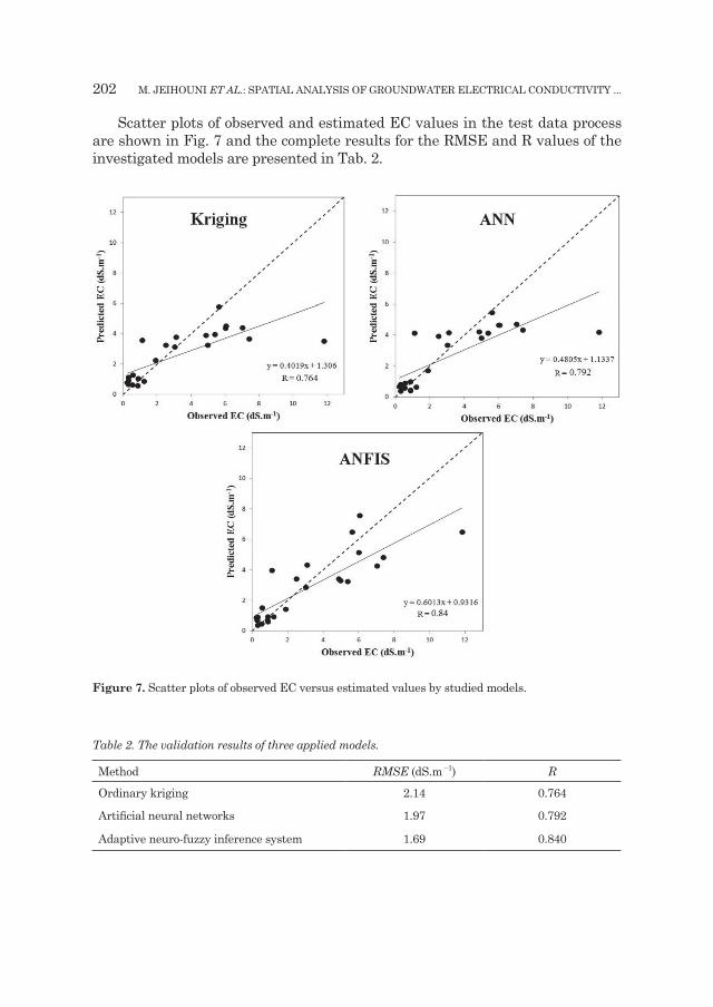
Scatter plots of observed and estimated EC values in the test data process are shown in Fig. 7 and the complete results for the RMSE and R values of the investigated models are presented in Tab. 2.

Figure 7. Scatter plots of observed EC versus estimated values by studied models.

Table 2. The validation results of three applied models.

Method RMSE (dS.m –1) R

Ordinary kriging 2.14 0.764

Artificial neural networks 1.97 0.792

Adaptive neuro-fuzzy inference system 1.69 0.840

GEOFIZIKA, vOl. 32, NO. 2, 2015, 191–208 203

As showed in Tab. 2, the ANFIS model had the minimum RMSE (1.69 dS.m–1) and maximum R (0.84) values between three investigated models. Conversely, OK had the relatively low accuracy due to high RMSE (2.14 dS.m–1 ) and low R (0.764) values. Also, from the Fig. 7 it is clear that the prediction of ANFIS model is closer to 1:1 line than those of the OK and ANN models. The ANN model esti-mations are also less scattered than the OK.

Comparison of different methods results is conducted based on keeping the principle of parsimony (keep the minimum, maximum, and median values of original data in interpolated values) as a box plot, and distribution of errors in the study area, in 2-d plot (Kazemi and hosseini, 2011). Box plot of observed and values interpolated by ANFIS, OK, and ANN are shown in Fig. 8. In this plot, the minimum, maximum, upper and lower quintiles of data are summarized.

Figure 8. Box plots of observed and interpolated values of EC using ANFIS, OK, and ANN.

Simulated maximum and minimum values based on three methods, are less than corresponding observed values. The three models are able to simulate the minimum values of contaminants but only the ANFIS’s maximum predicted val-ue was close to the observed maximum value. Median values of EC simulated by the three models were lower than observed median. In general, the range of pre-dicted values by ANFIS was wider than the range of OK and ANN predicted values.

Figure 9 shows observed and predicted values for validation period. It sug-gests that the ANFIS model generally performed better than the ANN and OK models, especially for the high EC values.

204 M. JEIhOuNI ET AL.: SpATIAl ANAlySIS OF GROuNdwATER ElECTRICAl CONduCTIvITy ...

Figure 9. performance of ANFIS, OK, and ANN models results in the testing period.

According to ANFIS performances (Tab. 2 and Figs. 8 and 9) it is seen that the non linear spatial interpolation methods can simulate complex spatial pat-terns better than other linear interpolation methods.

4. Conclusion

In this study, three spatial interpolation methods including linear estimator (OK) and artificial intelligence methods (ANN and ANFIS) were applied to esti-mate groundwater EC. Models were developed for predicting groundwater EC in a certain location based on its geographical coordinates. Comparisons were done between models outputs in order to select proper model. The results indicated that ANFIS model performed the best in comparison with other models. Further, ANN gave better results than OK. Accurate estimation of groundwater EC can help to improve environmental management and successful decision making in water quality problems. hence, it can be concluded that ANFIS method can be successfully employed in the study area to estimate groundwater EC.

References

Affandi, A. K. and watanabe, K. (2007): daily groundwater level fluctuation forecasting using soft computing technique, Nat. Sci., 5(2), 1–10.

Ahmadi, S. h. and Sedghamiz, A. (2007): Geostatistical analysis of spatial and temporal variations of groundwater level, Environ. Monit. Assess., 129, 277–294, dOI: 10.1007/s10661-006-9361-z.

GEOFIZIKA, vOl. 32, NO. 2, 2015, 191–208 205

Alsamamra, h., Ruiz-Arias, J. A., pozo-vázquez, d. and Tovar-pescador, J. (2009): A comparative study of ordinary and residual kriging techniques for mapping global solar radiation over south-ern Spain, Agric. For. Meteorol., 149, 1343–1357, dOI: 10.1016/j.agrformet.2009.03.005.

Alvisi, S., Mascellani, G., Franchini, M. and Bardossy, A. (2006): water level forecasting through fuzzy logic and artificial neural network approaches, J. Hydrol. Earth Syst. Sc., 10, 1–17, dOI: 10.5194/hessd-2-1107-2005.

Arslan, h. (2012): Spatial and temporal mapping of groundwater salinity using ordinary kriging and indicator kriging: The case of Bafra plain, Turkey, Agr. Water Manage., 113, 57–63, dOI: 10.1016/j.agwat.hh2012.06.015.

Buttner, O., Becker, A., Kellner, S., Kuehn, S., wendt- potthoff, K., Zachmann, d. w. and Friese, K. (1998): Geostatistical analysis of surface sediments in an acidic mining lake, Water Air Soil Poll., 108, 297– 316, dOI: 10.1023/A:1005145029916.

Cambardella, C. A., Moorman, T. B., Novak, J. M., parkin, T. B., Karlen, d. l., Turco, R. F., Konopka, A. E. (1994): Field-scale variability of soil properties in central Iowa soils, Soil Sci. Soc. Am. J., 58, 1501–1511.

Caro, A., legarda, F., Romero, l., herranz, M., Barrera, M., valiño, F., Idoeta, R. and Olondo, C. (2013): Map on predicted deposition of Cs-137 in Spanish soils from geostatistical analyses, J. Environ. Radioactiv., 115, 53–59, dOI: 10.1016/j.jenvrad.2012.06.007.

Cemek, B., Güler, M., Kılıç, K., demir, y. and Arslan, h. (2007): Assessment of spatial variability in some soil properties as related to soil salinity and alkalinity in Bafra plain in northern Turkey, Environ. Monit. Assess., 124, 223–234, dOI: 10.1007/s10661-006-9220-y.

Chandrasekharan, h., Sarangi, A., Nagarajan, M., Singh, v. p., Rao, d. u. M., Stalin, p., Natarajan, K., Chandrasekaran, B. and Anbazhagan, S. (2008): variability of soil-water quality due to Tsunami-2004 in the coastal belt of Nagapattinam district, Tamilnadu, J. Environ. Manage., 89, 63–72, dOI: 10.1016/j.jenvman.2007.01.051.

Chen, S. h., lin, y. h., Chang, l. C. and Chang, F. J. (2006): The strategy of building a flood forecast model by neuro-fuzzy networks, Hydrol. Progress., 20, 1525–1540, dOI: 10.1002/hyp.5942.

Cheng, C. B. and Lee, E. S. (1999): Applying fuzzy adaptive network to fuzzy regression analysis, Comput. Math. Appl., 38, 123–140, dOI: 10.1016/S0898-1221(99)00187-X.

Chowdhury, M., Alouani, A. and hossain, F. (2010): Comparison of ordinary kriging and artificial neural network for spatial mapping of arsenic contamination of groundwater, Stoch. Env. Res. Risk. A., 24, 1–7, dOI: 10.1007/s00477-008-0296-5.

dastorani, M. T., Moghadamnia, A., piri, J. and Rico-Ramirez., M. (2010): Application of ANN and ANFIS models for reconstructing missing flow data. Environ. Monit. Assess., 166, 421–434, dOI: 10.1007/s10661-009-1012-8.

duNing, X., li, X. y., Song, d. and yang, G. (2007): Temporal and spatial dynamical simulation of groundwater characteristics in Minqin Oasis, Sci. China, Ser. D., 50, 261–273, dOI: 10.1007/s11430-007-2001-9.

Flood, I. and Kartam, N. (1994): Neural networks in civil engineering. I: principles and understand-ing, J. Comput. Civil Eng., 8, 131–148, dOI: 10.1061/(ASCE)0887-3801(1994)8:2(131).

Gokalp, Z., Basaran, M., uzun, O. and Serin, y. (2010): Spatial analysis of some physical soil proper-ties in a saline and alkaline grassland soil of Kayseri, Turkey, Afr. J. Agr. Res., 5, 1127–1137.

Gringarten, E. and deutsch, C. v. (2001): Teacher’s aide variogram interpretation and modeling, Math. Geol, 33, 507–534, dOI: 10.1023/A:1011093014141.

Gupta, h. v., hsu, K. and Sorooshian, S. (2000): Effective and efficient modeling for streamflow fore-casting, in Chapter 1 of Artificial neural networks in hydrology, Govindaraju, R. S. and Rao, A. R. (Eds.), 7–22, Kluwer Academic publishers, Amesterdam, 348 pp.

206 M. JEIhOuNI ET AL.: SpATIAl ANAlySIS OF GROuNdwATER ElECTRICAl CONduCTIvITy ...

hasebe, M. and Nagayama, y. (2002): Reservoir operation using the neural network and fuzzy sys-tems for dam control and operation support, Adv. Eng. Softw., 335, 245–260, dOI: 10.1016/S0965-9978(02)00015-7.

hooshmand, A., delghandi, M., Izadi, A. and Aali, K. A. (2011): Application of kriging and cokriging in spatial estimation of groundwater quality parameters. Afr. J. Agr. Res., 6, 3402–3408, dOI: 10.5897/AJAR11.027.

hossain, F., hill, A. J. and Bagtzoglou, A. C. (2007): Geostatistically-based management of arsenic contaminated ground water in shallow wells of Bangladesh, Wat. Resour. Manage., 21, 1245–1261, dOI: 10.1007/s11269-006-9079-2.

Isaaks, E. h. and Srivastava, R. M. (1989): An introduction to applied geostatistics. Oxford univer. press, New york, 592 pp.

Jang, J. S. R. (1993): ANFIS: Adaptive network based fuzzy inference system. IEEE T. Sys. Man. Cyb., 23, 665–684, dOI: 10.1109/21.256541.

Jeihouni, M. Toomanian, A. Alavipanah, S. K., Shahabi, M. and Bazdar, S. (2015): An application of MC-SdSS for water supply management during a drought crisis, Environ. Monit. Assess., 187, 1–16, dOI: 10.1007/s10661-015-4643-y.

Jost, G., heuvelink, G. B. M. and papritz, A. (2005): Analysing the space–time distribution of soil water storage of a forest ecosystem using spatio-temporal kriging, Geoderma, 128, 258–273, dOI: 10.1016/j.geoderma.2005.04.008.

Kabiri-Samania A. R, Aghaee-Tarazjanib, J., Borgheic, S. M. and Jengd, d .S. (2011): Application of neural networks and fuzzy logic models to long-shore sediment transport, Appl. Soft Comput., 11, 2880–2887, dOI: 10.1016/j.asoc.2010.11.021.

Kazemi, S. M. and hosseini, S. M. (2011): Comparison of spatial interpolation methods for estimating heavy metals in sediments of Caspian Sea, Expert. Syst. Appl., 38, 1632–1649, dOI: 10.1016/j.eswa.2010.07.085.

Khashei-Siuki, A. and Sarbazi, M. (2013): Evaluation of ANFIS, ANN, and geostatistical models to spatial distribution of groundwater quality (case study: Mashhad plain in Iran), Arab. J. Geosci., 8, 903–912, dOI: 10.1007/s12517-013-1179-8.

Kholghi, M. and hosseini, S. M. (2009): Comparison of groundwater level estimation using neuro-fuzzy and ordinary kriging, Environ. Model. Assess., 14, 729–737, dOI: 10.1007/s10666-008- 9174-2.

Kisi, O. (2005): Suspended sediment estimation using neuro-fuzzy and neural network approaches, Hydrolog. Sci. J., 50, 683–696, dOI: 10.1623/hysj.2005.50.4.683.

Krishna, B., Satyaji Rao, y. R. and vijaya, T. (2008): Modeling groundwater levels in an urban coast-al aquifer using artificial neural networks, Hydrol. Process., 22, 1180–1188, dOI: 10.1002/hyp.6686.

Kumar, v. (2007): Optimal contour mapping of groundwater levels using universal kriging – a case study. Hydrolog. Sci. J., 52, 1039–1049, dOI: 10.1623/hysj.52.5.1038.

lallahem, S., Mania, J., hani, A. and Najjar, y. (2005): On the use of neural networks to evaluate groundwater levels in fracturedmedia, J. Hydrol., 307, 92–111, dOI: 10.1016/j.jhydrol. 2004.10.005.

lee, E. S. (2000): Neuro-fuzzy estimation in spatial statistics, J. Math. Anal. Appl., 249, 221–231, dOI: 10.1006/jmaa.2000.6938.

li, J., Cheng, J. h., Shi, J. y. and huang, F. (2012): Brief introduction of back propagation (Bp) neu-ral network algorithm and its improvement, in Advances in Computer Science and Information Engineering, Springer, Berlin, Germany, 553–558, dOI: 10.1007/978-3-642-30223-7_87.

GEOFIZIKA, vOl. 32, NO. 2, 2015, 191–208 207

McBratney, A. B., webster, R., Mclaren, R. G. and Spiers, R. B. (1982): Regional variation in extract-able copper and cobalt in the topsoil of south-east Scotland, Agron. Sustain. Dev., 2, 969–982, dOI: 10.1051/agro:19821010.

Nas, B. and Berktay, A. (2010): Groundwater quality mapping in urban groundwater using GIS, Environ. Monit. Assess., 160, 215–227, dOI: 10.1007/s10661-008-0689-4.

Nayak, p. C., Sudheer, K. p., Rangan, d. M., and Ramasastri, K. S., (2004): A neuro-fuzzy computing technique for modeling hydrological time series, J. Hydrol, 291, 52–66, dOI: 10.1016/j.jhydrol.2003.12.010.

Oliver, M. A., and webster, R. (2014): A tutorial guide to geostatistics: Computing and modelling variograms and kriging, Catena, 113, 56–69, dOI: 10.1016/j.catena.2013.09.006.

pektaş, A. O., and doğan, E. (2015): prediction of bed load via suspended sediment load using soft computing methods, Geofizika, 32, 27–46, dOI: 10.15233/gfz.2015.32.2.

poon, K., wong, R. w., lam, M. h., yeung, h. and Chiu, T. K. (2000): Geostatistical modelling of the spatial distribution of sewage pollution in coastal sediments, Water Res., 32, 99–108, dOI: 10.1016/S0043-1354(99)00119-0.

Ramsis, B. S., Claus, J. O. and Robert, w. F. (1999): Contributions of groundwater conditions to soil and water salinization, Hydrogeol. J., 7, 46–64, dOI: 10.1007/s100400050179.

Salas, J. d., Markus, M. and Tokar, A. S. (2000): Streamflow forecasting based on artificial neural networks, in Chapter 4 of Artificial neural networks in hydrology, Govindaraju, R. S. and Rao, A. R. (Eds.), 23–51, Kluwer Academic publishers, london, 348 pp.

Setnes, M., Babuska, R. and verbruggen, h. B. (1998): Transparent fuzzy modeling, Int. J. Hum.-Comput. St., 49, 159–179, dOI: 10.1006/ijhc.1998.0197.

Stein, M. l. (1999): Interpolation of spatial data: Some theory for kriging, Springer, New york, 249 pp.

Sun, y., Shaozhong, K., li, F. and Zhang, l. (2009): Comparison of interpolation methods for depth to groundwater and its temporal and spatial variations in the Minqin oasis of northwest China. Environ. Modell. Softw., 24, 1163–1170, dOI: 10.1016/j.envsoft.2009.03.009.

Theodossiou, N. and latinopoulos, p. (2007): Evaluation and optimisation of groundwater observa-tion networks using the Kriging methodology, Environ. Modell. Softw., 21, 991–1000, dOI: 10.1016/j.envsoft.2005.05.001.

Tutmez, B., hatipoglu, Z. and Kaymak, u. (2006): Modelling electrical conductivity of groundwater using an adaptive neuro-fuzzy inference system, Comput. Geosci., 32, 421–433, dOI: 10.1016/j.cageo.2005.07.003.

uyan, M. and Cay, T. (2013): Spatial analyses of groundwater level differences using geostatistical modeling. Environ. Ecol. Stat., 20, 633–646, dOI: 10.1007/s10651-013-0238-3.

yesilnacar, M. I. and Sahinkaya, E. (2012): Artificial neural network prediction of sulfate and SAR in an unconfined aquifer in southeastern Turkey, Environ. Earth Sci., 67, 1111–1119, dOI: 10.1007/s12665-012-1555-9.

yesilnacar, M. I., Şahinkaya, E., Naz, M. and Ozkaya, B. (2008): Neural Network prediction of Nitrate in Groundwater of harran plain, Turkey, Environ. Geol., 56, 19–25, dOI: 10.1007/s00254-007-1136-5.

yimit, h., Eziz, M., Mamat, M. and Tohti, G. (2011): variations in groundwater levels and salinity in the Ili River Irrigation Area, Xinjiang, northwest China: A geostatistical approach, Int. J. Sust. Dev. World Ecol., 18, 55–64, dOI: 10.1080/13504509.2011.544871.

208 M. JEIhOuNI ET AL.: SpATIAl ANAlySIS OF GROuNdwATER ElECTRICAl CONduCTIvITy ...

SAŽETAK

Prostorna analiza električne vodljivosti podzemnih voda pomoću običnoga kriginga i metoda umjetne inteligencije

(slučaj ravnice Tabriz, Iran)

Mehrdad Jeihouni, Reza Delirhasannia, Seyed Kazem Alavipanah, Mahmoud Shahabi i Saeed Samadianfard

u posljednjih nekoliko desetljeća sustavi umjetne inteligencije (AI) su otvorili nove horizonte u analizi problema vodnog inženjeringa te ekoloških problema. u ovoj studiji istražene su performanse običnog kriginga (OK) kao geostatističkog procjenitelja te per-formanse dvaju naprednih metoda, prva od kojih je umjetna neuronska mreža (ANN), a druga je hibridni sustav ANFIS (Adaptive Neuro-Fuzzy Inference System) koji uz neuron-sku mrežu uključuje i neizravnu (fuzzy) logiku. u tu svrhu, zemljopisne koordinate 120 mjernih bunara lociranih u ravnici Tabriz u sjeverozapadnom Iranu definirane su kao ulazi, a električne vodljivosti (EC) podzemnih voda postavljeni su kao izlazi modela. Osamdeset posto podataka nasumce je izabrano za razvoj i obuku (učenje) navedenih modela, a dvadeset posto podataka iskorišteno je za testiranje i provjeru. Na kraju, izlazi modela su uspoređeni s odgovarajućim mjerenim vrijednostima u mjernim bunarima. Rezultati su pokazali da model ANFIS među svim promatranim modelima daje najbolju točnost s korijenom srednje kvadratne pogreške (RMSE) od 1,69 dS.m–1 i koeficijentom korelacije (R) od 0,84. Izračunate vrijednosti RMSE u modelima ANN i OK iznose 1.97, odnosno 2.14 dS.m–1, a koeficijenata korelacije 0,79, odnosno 0,76, respektivno. prema dobivenim rezultatima ANFIS metoda je precizno predvidjela električnu vodljivost te se stoga može preporučiti za modeliranje saliniteta podzemnih voda.

Ključne riječi: umjetna inteligencija, obični kriging, električna vodljivost, ravnica Tabriz, podzemne vode

Corresponding author’s address: Mehrdad Jeihouni; tel: +989 1 4100 7411; e-mail: jeihouni92@ut.ac.ir