Sparse Regression Codes - ISIT 2016 BarcelonaOutline of Tutorial Sparse Superposition Codes or...
64
. . . . . . . . . . . . . . . . . . . . . . . . . . . . . . . . . . . . . . . . Sparse Regression Codes Andrew Barron Ramji Venkataramanan Yale University University of Cambridge Joint work with Antony Joseph, Sanghee Cho, Cynthia Rush, Adam Greig, Tuhin Sarkar, Sekhar Tatikonda ISIT 2016 1 / 57
Transcript of Sparse Regression Codes - ISIT 2016 BarcelonaOutline of Tutorial Sparse Superposition Codes or...
.
.
.
.
.
.
.
.
.
.
.
.
.
.
.
.
.
.
.
.
.
.
.
.
.
.
.
.
.
.
.
.
.
.
.
.
.
.
.
.
Sparse Regression Codes
Andrew Barron Ramji Venkataramanan
Yale University University of Cambridge
Joint work with Antony Joseph, Sanghee Cho, Cynthia Rush,Adam Greig, Tuhin Sarkar, Sekhar Tatikonda
ISIT 2016
1 / 57

.
.
.
.
.
.
.
.
.
.
.
.
.
.
.
.
.
.
.
.
.
.
.
.
.
.
.
.
.
.
.
.
.
.
.
.
.
.
.
.
Outline of Tutorial
Sparse Superposition Codes or Sparse Regression Codes (SPARCs)for:
1. Provably practical and reliable communication over theAWGN channel at rates approaching capacity
2. Efficient lossy compression at rates approaching Shannon limit
3. Multi-terminal communication and compression models
4. Open Questions
2 / 57

.
.
.
.
.
.
.
.
.
.
.
.
.
.
.
.
.
.
.
.
.
.
.
.
.
.
.
.
.
.
.
.
.
.
.
.
.
.
.
.
Part I: Communication over theAWGN Channel
3 / 57

.
.
.
.
.
.
.
.
.
.
.
.
.
.
.
.
.
.
.
.
.
.
.
.
.
.
.
.
.
.
.
.
.
.
.
.
.
.
.
.
Quest for Provably Practical and Reliable High RateCommunication
• The Channel Communication Problem
• Gaussian Channel
• History of Methods
• Sparse Superposition Coding
• Three efficient decoders:
1. Adaptive successive threshold decoder2. Adaptive successive soft-decision decoder3. Approximate Message Passing (AMP) decoder
• Rate, Reliability, and Computational Complexity
• Distributional Analysis
• Simulations
4 / 57
.
.
.
.
.
.
.
.
.
.
.
.
.
.
.
.
.
.
.
.
.
.
.
.
.
.
.
.
.
.
.
.
.
.
.
.
.
.
.
.
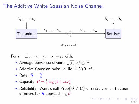
The Additive White Gaussian Noise Channel
Transmitter
U1, . . . ,UK
ε1, . . . , εn
x1, . . . , xnReceiver
y1, . . . , yn
U1, . . . , UK
For i = 1, . . . n, yi = xi + εi with:
• Average power constraint: 1n
∑i x
2i ≤ P
• Additive Gaussian noise: εi iid ∼ N (0, σ2)
• Rate: R = Kn
• Capacity: C = 12 log (1 + snr)
• Reliability: Want small Prob{U = U} or reliably small fractionof errors for R approaching C
5 / 57
.
.
.
.
.
.
.
.
.
.
.
.
.
.
.
.
.
.
.
.
.
.
.
.
.
.
.
.
.
.
.
.
.
.
.
.
.
.
.
.
Capacity-achieving codes
For many binary/discrete alphabet channels:
• Turbo and sparse-graph (LDPC) codes achieve rates close tocapacity with efficient message-passing decoding
• Theoretical results for spatially-coupled LDPC codes[Kudekar, Richardson, Urbanke ’12, ’13], . . .
• Polar codes achieve capacity with efficient decoding[Arikan ’09], [Arikan, Telatar], . . .
But we want to achieve C for the AWGN channel. Let’s lookat some existing approaches . . .
6 / 57

.
.
.
.
.
.
.
.
.
.
.
.
.
.
.
.
.
.
.
.
.
.
.
.
.
.
.
.
.
.
.
.
.
.
.
.
.
.
.
.
Existing Approaches: Coded Modulation
U = (U1 . . .UK )
Channel Encoder
Modulator
c1, . . . , cm
ε1 . . . εn
x1 . . . xnDemodulator
y1 . . . yn
Channel Decoder
U = (U1 . . . UK )
1. Fix a modulation scheme, e.g, 16-QAM, 64-QAM
2. Use a powerful binary code (e.g., LDPC, turbo code) toprotect against errors
3. Channel decoder uses soft outputs from demodulator
Surveys:[Ungerboeck, Forney’98], [Guillen i Fabregas, Martinez, Caire’08]7 / 57

.
.
.
.
.
.
.
.
.
.
.
.
.
.
.
.
.
.
.
.
.
.
.
.
.
.
.
.
.
.
.
.
.
.
.
.
.
.
.
.
Existing Approaches: Coded Modulation
U = (U1 . . .UK )
Channel Encoder
Modulator
c1, . . . , cm
ε1 . . . εn
x1 . . . xnDemodulator
y1 . . . yn
Channel Decoder
U = (U1 . . . UK )
Coded modulation works well in practice, but cannot provablyachieve capacity with fixed constellation
7 / 57
.
.
.
.
.
.
.
.
.
.
.
.
.
.
.
.
.
.
.
.
.
.
.
.
.
.
.
.
.
.
.
.
.
.
.
.
.
.
.
.
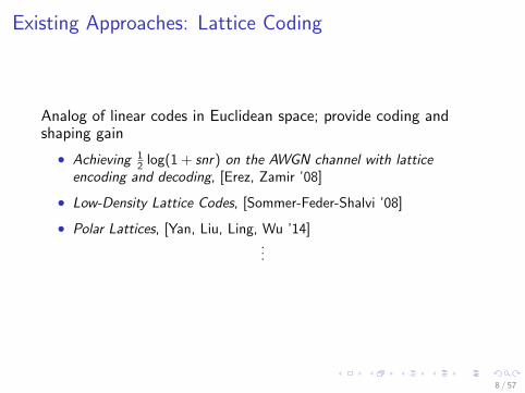
Existing Approaches: Lattice Coding
Analog of linear codes in Euclidean space; provide coding andshaping gain
• Achieving 12 log(1 + snr) on the AWGN channel with lattice
encoding and decoding, [Erez, Zamir ’08]
• Low-Density Lattice Codes, [Sommer-Feder-Shalvi ’08]
• Polar Lattices, [Yan, Liu, Ling, Wu ’14]...
8 / 57

.
.
.
.
.
.
.
.
.
.
.
.
.
.
.
.
.
.
.
.
.
.
.
.
.
.
.
.
.
.
.
.
.
.
.
.
.
.
.
.
Sparse Regression Codes (SPARC)
In this part of the tutorial, we discuss the basic Sparse RegressionCode construction with power allocation + two feasible decoders
References for this part:
– A. Joseph and A. R. Barron, Least-squares superposition codes ofmoderate dictionary are reliable at rates up to capacity, IEEE Trans. Inf.Theory, May 2012
– A. Joseph and A. R. Barron, Fast sparse superposition codes have nearexponential error probability for R < C, IEEE Trans. Inf. Theory, Feb.2014
– A. R. Barron and S. Cho, High-rate sparse superposition codes withiteratively optimal estimates, ISIT 2012
– A. R. Barron and S. Cho, Approximate Iterative Bayes OptimalEstimates for High-Rate Sparse Superposition Codes, WITMSE 2013
– S. Cho, High-dimensional regression with random design, includingsparse superposition codes, PhD thesis, Yale University, 2014
9 / 57

.
.
.
.
.
.
.
.
.
.
.
.
.
.
.
.
.
.
.
.
.
.
.
.
.
.
.
.
.
.
.
.
.
.
.
.
.
.
.
.
Extensions and Generalizations of SPARCs
Spatially-coupled dictionaries for SPARC:J. Barbier, C. Schulke, F. Krzakala, Approximate message-passing with
spatially coupled structured operators, with applications to compressed
sensing and sparse superposition codes, J. Stat. Mech, 2015
http://arxiv.org/abs/1503.08040
Bernoulli ±1 dictionaries:Y. Takeishi, M. Kawakita, and J. Takeuchi. Least squares superposition
codes with bernoulli dictionary are still reliable at rates up to capacity ,
IEEE Trans. Inf. Theory, May 2014
Tuesday afternoon session on Sparse Superposition Codes
10 / 57
.
.
.
.
.
.
.
.
.
.
.
.
.
.
.
.
.
.
.
.
.
.
.
.
.
.
.
.
.
.
.
.
.
.
.
.
.
.
.
.
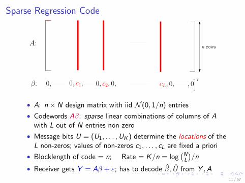
Sparse Regression Code
A:
β: 0, c1, 0, c2, 0, cL, 0, , 00,T
n rows
• A: n × N design matrix with iid N (0, 1/n) entries
• Codewords Aβ: sparse linear combinations of columns of Awith L out of N entries non-zero
• Message bits U = (U1, . . . ,UK ) determine the locations of theL non-zeros; values of non-zeros c1, . . . , cL are fixed a priori
• Blocklength of code = n; Rate = K/n = log(NL
)/n
• Receiver gets Y = Aβ + ε; has to decode β, U from Y ,A
11 / 57
.
.
.
.
.
.
.
.
.
.
.
.
.
.
.
.
.
.
.
.
.
.
.
.
.
.
.
.
.
.
.
.
.
.
.
.
.
.
.
.
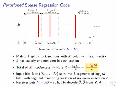
Partitioned Sparse Regression Code
A:
β: 0, c2, 0, cL, 0, , 00,
M columns M columnsM columnsSection 1 Section 2 Section L
T
n rows
0, c1,
Number of columns N = ML
• Matrix A split into L sections with M columns in each section• β has exactly one non-zero in each section
• Total of ML codewords ⇒ Rate R = logML
n =L logM
n• Input bits U = (U1, . . . ,UK ) split into L segments of log2Mbits, with segment ℓ indexing location of non-zero in section ℓ
• Receiver gets Y = Aβ + ε; has to decode β, U from Y ,A12 / 57

.
.
.
.
.
.
.
.
.
.
.
.
.
.
.
.
.
.
.
.
.
.
.
.
.
.
.
.
.
.
.
.
.
.
.
.
.
.
.
.
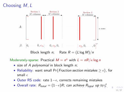
Choosing M , L
A:
β: 0, c2, 0, cL, 0, , 00,
M columns M columnsM columnsSection 1 Section 2 Section L
T
n rows
0, c1,
Block length n; Rate R = (L logM)/n
Ultra-sparse case: Impractical M = 2nR/L with L constant
• Reliable at all rates R < C [Cover 1972,1980]
• But size of A exponential in block length n
13 / 57
.
.
.
.
.
.
.
.
.
.
.
.
.
.
.
.
.
.
.
.
.
.
.
.
.
.
.
.
.
.
.
.
.
.
.
.
.
.
.
.
Choosing M , L
A:
β: 0, c2, 0, cL, 0, , 00,
M columns M columnsM columnsSection 1 Section 2 Section L
T
n rows
0, c1,
Block length n; Rate R = (L logM)/n
Moderately-sparse: Practical M = nκ with L = nR/κ log n
• size of A polynomial in block length n;
• Reliability: want small Pr{Fraction section mistakes ≥ ϵ}, forsmall ϵ
• Outer RS code: rate 1−ϵ, corrects remaining mistakes
• Overall rate: Rtotal = (1−ϵ)R; can achieve Rtotal up to C13 / 57
.
.
.
.
.
.
.
.
.
.
.
.
.
.
.
.
.
.
.
.
.
.
.
.
.
.
.
.
.
.
.
.
.
.
.
.
.
.
.
.
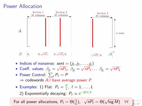
Power Allocation
A:
�: 0,pnP2, 0,
pnPL, 0, , 00,
M columns M columns
M columns
Section 1 Section 2
Section L
T
n rows
0,pnP1,
• Indices of nonzeros: sent = (j1, j2, . . . , jL)• Coeff. values: βj1 =
√nP1, βj2 =
√nP2 . . . βjL =
√nPL
• Power Control:∑
ℓ Pℓ = P⇒ codewords Aβ have average power P
• Examples: 1) Flat: Pℓ =PL , ℓ = 1, . . . , L
2) Exponentially decaying: Pℓ ∝ e−2Cℓ/L
For all power allocations, Pℓ = Θ( 1L),√nPℓ = Θ(
√logM) ∀ℓ
14 / 57

.
.
.
.
.
.
.
.
.
.
.
.
.
.
.
.
.
.
.
.
.
.
.
.
.
.
.
.
.
.
.
.
.
.
.
.
.
.
.
.
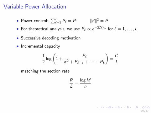
Variable Power Allocation
• Power control:∑L
ℓ=1 Pℓ = P ∥β∥2 = P
• Variable power: Pℓ proportional to e−2Cℓ/L for ℓ = 1, . . . , L
Example: P=7, L = 100
0 20 40 60 80 100
0.000
0.005
0.010
0.015
0.020
section index
pow
er a
lloca
tion
15 / 57
.
.
.
.
.
.
.
.
.
.
.
.
.
.
.
.
.
.
.
.
.
.
.
.
.
.
.
.
.
.
.
.
.
.
.
.
.
.
.
.
Variable Power Allocation
• Power control:∑L
ℓ=1 Pℓ = P ∥β∥2 = P
• For theoretical analysis, we use Pℓ ∝ e−2Cℓ/L for ℓ = 1, . . . , L
• Successive decoding motivation
• Incremental capacity
1
2log
(1 +
Pℓ
σ2 + Pℓ+1 + · · ·+ PL
)=
CL
matching the section rate
R
L=
logM
n
16 / 57

.
.
.
.
.
.
.
.
.
.
.
.
.
.
.
.
.
.
.
.
.
.
.
.
.
.
.
.
.
.
.
.
.
.
.
.
.
.
.
.
Decoding
A:
�: 0,pnP2, 0,
pnPL, 0, , 00,
M columns M columns
M columns
Section 1 Section 2
Section L
T
n rows
0,pnP1,
GOAL: Recover sent terms in β, i.e., non-zero indices j1, . . . , jLfrom
Y = Aβ + ε
• Optimal decoder (ML): βML = argminβ ∥Y − Aβ∥2. Butcomplexity exponential in n
• Feasible decoders: We will present three decoders, each ofwhich iteratively produces estimates of β denoted β1, β2, . . .
17 / 57

.
.
.
.
.
.
.
.
.
.
.
.
.
.
.
.
.
.
.
.
.
.
.
.
.
.
.
.
.
.
.
.
.
.
.
.
.
.
.
.
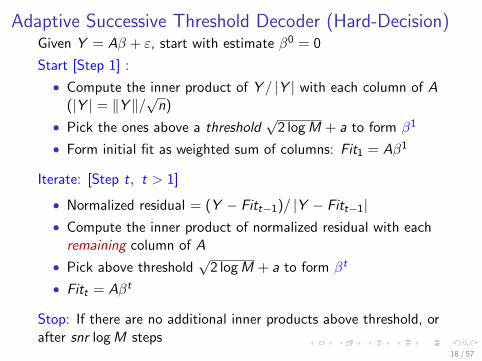
Adaptive Successive Threshold Decoder (Hard-Decision)Given Y = Aβ + ε, start with estimate β0 = 0
Start [Step 1] :
• Compute the inner product of Y / |Y | with each column of A(|Y | = ∥Y ∥/
√n)
• Pick the ones above a threshold√2 logM + a to form β1
• Form initial fit as weighted sum of columns: Fit1 = Aβ1
Iterate: [Step t, t > 1]
• Normalized residual = (Y − Fitt−1)/ |Y − Fitt−1|• Compute the inner product of normalized residual with eachremaining column of A
• Pick above threshold√2 logM + a to form βt
• Fitt = Aβt
Stop: If there are no additional inner products above threshold, orafter snr logM steps
18 / 57
.
.
.
.
.
.
.
.
.
.
.
.
.
.
.
.
.
.
.
.
.
.
.
.
.
.
.
.
.
.
.
.
.
.
.
.
.
.
.
.
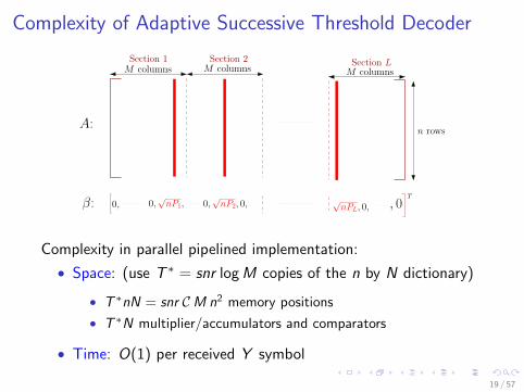
Complexity of Adaptive Successive Threshold Decoder
A:
�: 0,pnP2, 0,
pnPL, 0, , 00,
M columns M columns
M columns
Section 1 Section 2
Section L
T
n rows
0,pnP1,
Complexity in parallel pipelined implementation:
• Space: (use T ∗ = snr logM copies of the n by N dictionary)
• T ∗nN = snr CM n2 memory positions
• T ∗N multiplier/accumulators and comparators
• Time: O(1) per received Y symbol
19 / 57
.
.
.
.
.
.
.
.
.
.
.
.
.
.
.
.
.
.
.
.
.
.
.
.
.
.
.
.
.
.
.
.
.
.
.
.
.
.
.
.
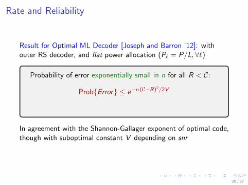
Rate and Reliability
Result for Optimal ML Decoder [Joseph and Barron ’12]: withouter RS decoder, and flat power allocation (Pℓ = P/L, ∀ℓ)
Probability of error exponentially small in n for all R < C:
Prob{Error} ≤ e−n (C−R)2/2V
In agreement with the Shannon-Gallager exponent of optimal code,though with suboptimal constant V depending on snr
20 / 57

.
.
.
.
.
.
.
.
.
.
.
.
.
.
.
.
.
.
.
.
.
.
.
.
.
.
.
.
.
.
.
.
.
.
.
.
.
.
.
.
Performance of Adaptive Successive Threshold Decoder
Practical: Adaptive Successive Decoder, with outer RS code.
[Joseph-Barron]:
• Value CM approaching capacity:
CM = C(1− c1
logM
)
Probability error exponentially small in L for R < CM
Prob{Error
}≤ e−L(CM−R)2c2
• L ∼ n/(log n)⇒ Prob error exponentially small in n/(log n) for R < C
21 / 57

.
.
.
.
.
.
.
.
.
.
.
.
.
.
.
.
.
.
.
.
.
.
.
.
.
.
.
.
.
.
.
.
.
.
.
.
.
.
.
.
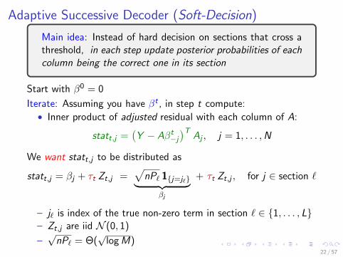
Adaptive Successive Decoder (Soft-Decision)
Main idea: Instead of hard decision on sections that cross athreshold, in each step update posterior probabilities of eachcolumn being the correct one in its section
Start with β0 = 0
Iterate: Assuming you have βt , in step t compute:• Inner product of adjusted residual with each column of A:
statt,j =(Y − Aβt
−j
)TAj , j = 1, . . . ,N
We want statt,j to be distributed as
statt,j = βj + τt Zt,j =√
nPℓ 1{j=jℓ}︸ ︷︷ ︸βj
+ τt Zt,j , for j ∈ section ℓ
– jℓ is index of the true non-zero term in section ℓ ∈ {1, . . . , L}– Zt,j are iid N (0, 1)
–√nPℓ = Θ(
√logM)
22 / 57
.
.
.
.
.
.
.
.
.
.
.
.
.
.
.
.
.
.
.
.
.
.
.
.
.
.
.
.
.
.
.
.
.
.
.
.
.
.
.
.
Adaptive Successive Decoder (Soft-Decision)
Main idea: Instead of hard decision on sections that cross athreshold, in each step update posterior probabilities of eachcolumn being the correct one in its section
Start with β0 = 0
Iterate: Assuming you have βt , in step t compute:• Inner product of adjusted residual with each column of A:
statt,j =(Y − Aβt
−j
)TAj , j = 1, . . . ,N
We want statt,j to be distributed as
statt,j = βj + τt Zt,j =√
nPℓ 1{j=jℓ}︸ ︷︷ ︸βj
+ τt Zt,j , for j ∈ section ℓ
– jℓ is index of the true non-zero term in section ℓ ∈ {1, . . . , L}– Zt,j are iid N (0, 1)
–√nPℓ = Θ(
√logM)
22 / 57

.
.
.
.
.
.
.
.
.
.
.
.
.
.
.
.
.
.
.
.
.
.
.
.
.
.
.
.
.
.
.
.
.
.
.
.
.
.
.
.
Iteratively Bayes Optimal EstimatesThe Bayes estimate based on statt is β
t+1 = E[β|statt ] with:• statt,j =
√nPℓ 1{j=jℓ} + τt Zt,j , for j ∈ sec. ℓ
• Prior jℓ ∼ Uniform on indices in sec. ℓ, Zt,j iid ∼ N (0, 1)
For j ∈ section ℓ:
βt+1j (s) = E[βj |statt = s] =
√nPℓ Prob(jℓ = j | statt = s)
=√
nPℓexp(
√nPℓ sj/τ
2t )∑
k∈secℓ exp(√nPℓ sk/τ
2t )︸ ︷︷ ︸
wj (τt)
Weight wj(τt) is the posterior probability (after step t) ofcolumn j being the correct one in its section
23 / 57

.
.
.
.
.
.
.
.
.
.
.
.
.
.
.
.
.
.
.
.
.
.
.
.
.
.
.
.
.
.
.
.
.
.
.
.
.
.
.
.
Desired Distribution
All of this is based on the desired distribution of statt :
statt,j =√
nPℓ 1{j=jℓ}︸ ︷︷ ︸βj
+ τt Zt,j , for j ∈ section ℓ
What is the noise variance τ2t ?
We can write
statt,j = (Y − Aβt−j)
TAj = (Y − Aβt)TAj + ∥Aj∥2︸ ︷︷ ︸≈1
βtj
Hence
statt = (Y −Aβt)TAj + βt = β + ATw︸ ︷︷ ︸N (0,σ2)
+ (I− ATA)︸ ︷︷ ︸≈N (0,1/n)
(βt − β)
If (β − βt) were independent of (I− ATA), then . . .24 / 57

.
.
.
.
.
.
.
.
.
.
.
.
.
.
.
.
.
.
.
.
.
.
.
.
.
.
.
.
.
.
.
.
.
.
.
.
.
.
.
.
Noise Variance τ 2tIf (β − βt) were independent of (I− ATA), then:
statt = β + τt Zt
where
τ2t = σ2 +1
nE ∥β − βt∥2
Assuming stat1, . . . , statt−1 are all distributed as desired, then
1
nE ∥β − βt∥2 = 1
nE ∥β − E[β|β + τt−1Zt−1]∥2 = P(1− xt(τt−1))
where
xt(τt−1) =L∑
ℓ=1
Pℓ
PE
[exp
(√nPℓ
τt−1(Uℓ
1 +√nPℓ
τt−1))
exp(√
nPℓτt−1
(Uℓ1 +
√nPℓ
τt−1))+∑M
j=2 exp(√
nPℓτt−1
Uℓj
)]
{Uℓj } are i.i.d. ∼ N (0, 1)
25 / 57

.
.
.
.
.
.
.
.
.
.
.
.
.
.
.
.
.
.
.
.
.
.
.
.
.
.
.
.
.
.
.
.
.
.
.
.
.
.
.
.
Iteratively compute variances τ 2t
τ20 = σ2 + P
τ2t = σ2 + P(1− xt(τt−1)), t ≥ 1
where
xt(τt−1) =L∑
ℓ=1
Pℓ
PE
[exp
(√nPℓ
τt−1(Uℓ
1 +√nPℓ
τt−1))
exp(√
nPℓτt−1
(Uℓ1 +
√nPℓ
τt−1))+∑M
j=2 exp(√
nPℓτt−1
Uℓj
)︸ ︷︷ ︸
wjℓ(τt−1)
]
With statt = β + τtZ :
1n E∥β − βt∥2 = P(1− xt) and 1
n E[βTβt ] = 1
n E∥βt∥2 = Pxt
• xt : Expected power-weighted fraction of correctlydecoded sections after step t
• P(1− xt): interference due to undecoded sections
26 / 57

.
.
.
.
.
.
.
.
.
.
.
.
.
.
.
.
.
.
.
.
.
.
.
.
.
.
.
.
.
.
.
.
.
.
.
.
.
.
.
.
Update Rule for Success Rate xt
1) Update rule xt = g(xt−1) where
g(x) =L∑
ℓ=1
Pℓ
PE
[exp
(√nPℓτ (Uℓ
1 +√nPℓτ )
)exp
(√nPℓτ (Uℓ
1 +√nPℓτ )
)+∑M
j=2 exp(√
nPℓτ Uℓ
j
)︸ ︷︷ ︸
wjℓ(τ)
]
with τ2 = σ2 + P(1− x).
This is the success rate update function expressed as apower-weighted sum of the posterior prob of the term sent
Under the assumed distribution of statt :
2) The true empirical success rate is x∗t = 1nPβ
Tβt
3) The decoder could also compute the empirical estimatedsuccess rate xt =
1nP ∥β
t∥2
27 / 57
.
.
.
.
.
.
.
.
.
.
.
.
.
.
.
.
.
.
.
.
.
.
.
.
.
.
.
.
.
.
.
.
.
.
.
.
.
.
.
.
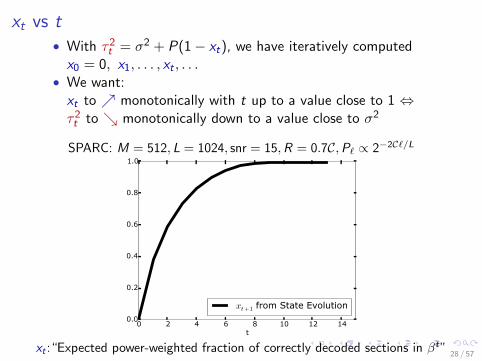
xt vs t• With τ2t = σ2 + P(1− xt), we have iteratively computedx0 = 0, x1, . . . , xt , . . .
• We want:xt to ↗ monotonically with t up to a value close to 1 ⇔τ2t to ↘ monotonically down to a value close to σ2
SPARC: M = 512, L = 1024, snr = 15,R = 0.7C,Pℓ ∝ 2−2Cℓ/L
xt :“Expected power-weighted fraction of correctly decoded sections in βt”28 / 57

.
.
.
.
.
.
.
.
.
.
.
.
.
.
.
.
.
.
.
.
.
.
.
.
.
.
.
.
.
.
.
.
.
.
.
.
.
.
.
.
Decoding Progression: g(x) vs x
0.0 0.2 0.4 0.6 0.8 1.0
0.0
0.2
0.4
0.6
0.8
1.0
x
M = 29 , L =Msnr=7C=1.5 bitsR=1.2 bits(0.8C)
g(x)x
29 / 57
.
.
.
.
.
.
.
.
.
.
.
.
.
.
.
.
.
.
.
.
.
.
.
.
.
.
.
.
.
.
.
.
.
.
.
.
.
.
.
.
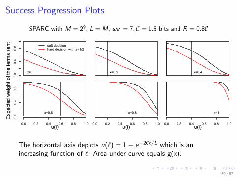
Success Progression Plots
SPARC with M = 29, L = M, snr = 7, C = 1.5 bits and R = 0.8C
0.0
0.4
0.8
x
Exp
ecte
d w
eigh
t of t
he te
rms
sent
x=0
soft decisionhard decision with a=1/2
x
x=0.2
x
x=0.4
0.0 0.2 0.4 0.6 0.8 1.0
0.0
0.4
0.8
xu(l)
x=0.6
0.0 0.2 0.4 0.6 0.8 1.0
xu(l)
x=0.8
0.0 0.2 0.4 0.6 0.8 1.0
xu(l)
x=1
The horizontal axis depicts u(ℓ) = 1− e−2Cℓ/L which is anincreasing function of ℓ. Area under curve equals g(x).
30 / 57
.
.
.
.
.
.
.
.
.
.
.
.
.
.
.
.
.
.
.
.
.
.
.
.
.
.
.
.
.
.
.
.
.
.
.
.
.
.
.
.
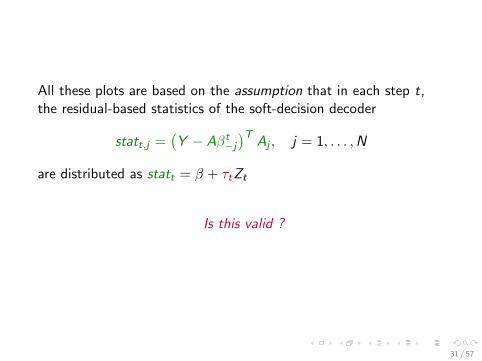
All these plots are based on the assumption that in each step t,the residual-based statistics of the soft-decision decoder
statt,j =(Y − Aβt
−j
)TAj , j = 1, . . . ,N
are distributed as statt = β + τtZt
Is this valid ?
31 / 57

.
.
.
.
.
.
.
.
.
.
.
.
.
.
.
.
.
.
.
.
.
.
.
.
.
.
.
.
.
.
.
.
.
.
.
.
.
.
.
.
SimulationSPARC: L = 512,M = 64, snr = 15, C = 2 bits, R = 1 bit (n = 3072)
xt vs xt−1
Green lines for hard thresholding; blue and red for soft decisiondecoder. Ran 20 trials for each method.
32 / 57

.
.
.
.
.
.
.
.
.
.
.
.
.
.
.
.
.
.
.
.
.
.
.
.
.
.
.
.
.
.
.
.
.
.
.
.
.
.
.
.
Clearly, empirical success rate xt does not follow theoretical curve⇒ Residual-based statt is not well-approximated by β + τtZ !
How to form statt that is close to the desired representation?
33 / 57

.
.
.
.
.
.
.
.
.
.
.
.
.
.
.
.
.
.
.
.
.
.
.
.
.
.
.
.
.
.
.
.
.
.
.
.
.
.
.
.
Recall: Once statt has the representation statt = β + τtZt , it’seasy to produce Bayes optimal estimate:
For j ∈ section ℓ:
βt+1j (statt = s) = E[βj |statt = s] =
√nPℓ
exp(√nPℓ sj/τ
2t )∑
k∈secℓ exp(√nPℓ sk/τ
2t )︸ ︷︷ ︸
wj (τt)
34 / 57

.
.
.
.
.
.
.
.
.
.
.
.
.
.
.
.
.
.
.
.
.
.
.
.
.
.
.
.
.
.
.
.
.
.
.
.
.
.
.
.
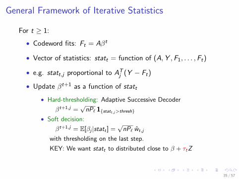
General Framework of Iterative Statistics
For t ≥ 1:
• Codeword fits: Ft = Aβt
• Vector of statistics: statt = function of (A,Y ,F1, . . . ,Ft)
• e.g. statt,j proportional to ATj (Y − Ft)
• Update βt+1 as a function of statt
• Hard-thresholding: Adaptive Successive Decoder
βt+1,j =√nPℓ 1{statt,j>thresh}
• Soft decision:
βt+1,j = E[βj |statt ] =√nPℓ wt,j
with thresholding on the last step.
KEY: We want statt to distributed close to β + τtZ
35 / 57
.
.
.
.
.
.
.
.
.
.
.
.
.
.
.
.
.
.
.
.
.
.
.
.
.
.
.
.
.
.
.
.
.
.
.
.
.
.
.
.
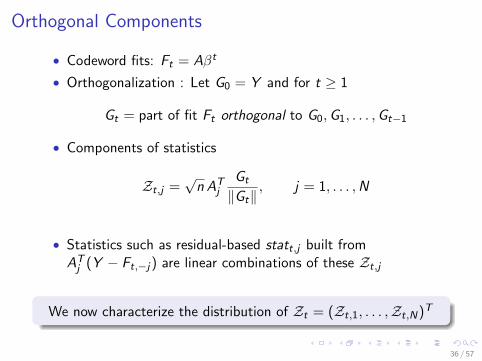
Orthogonal Components
• Codeword fits: Ft = Aβt
• Orthogonalization : Let G0 = Y and for t ≥ 1
Gt = part of fit Ft orthogonal to G0,G1, . . . ,Gt−1
• Components of statistics
Zt,j =√n AT
j
Gt
∥Gt∥, j = 1, . . . ,N
• Statistics such as residual-based statt,j built fromATj (Y − Ft,−j) are linear combinations of these Zt,j
We now characterize the distribution of Zt = (Zt,1, . . . ,Zt,N)T
36 / 57
.
.
.
.
.
.
.
.
.
.
.
.
.
.
.
.
.
.
.
.
.
.
.
.
.
.
.
.
.
.
.
.
.
.
.
.
.
.
.
.
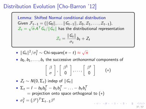
Distribution Evolution [Cho-Barron ’12]
Lemma: Shifted Normal conditional distributionGiven Ft−1 = (∥G0∥, . . . ∥Gt−1∥,Z0,Z1, . . . ,Zt−1),Zt =
√n ATGt/∥Gt∥ has the distributional representation
Zt =∥Gt∥σt
bt + Zt
• ∥Gt∥2/σ2t ∼ Chi-square(n − t) ≈
√n
• b0, b1, . . . , bt the successive orthonormal components of[βσ
],
[β1
0
], . . . ,
[βt
0
](∗)
• Zt ∼ N(0,Σt) indep of ∥Gt∥• Σt = I − b0b
T0 − b1b
T1 − . . .− btb
Tt
= projection onto space orthogonal to (∗)• σ2
t = (βt)TΣt−1βt
37 / 57
.
.
.
.
.
.
.
.
.
.
.
.
.
.
.
.
.
.
.
.
.
.
.
.
.
.
.
.
.
.
.
.
.
.
.
.
.
.
.
.
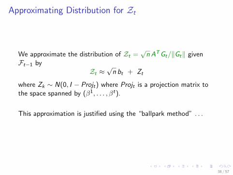
Approximating Distribution for Zt
We approximate the distribution of Zt =√n ATGt/∥Gt∥ given
Ft−1 byZt ≈
√n bt + Zt
where Zk ∼ N(0, I − Projt) where Projt is a projection matrix tothe space spanned by (β1, . . . , βt).
This approximation is justified using the “ballpark method” . . .
38 / 57

.
.
.
.
.
.
.
.
.
.
.
.
.
.
.
.
.
.
.
.
.
.
.
.
.
.
.
.
.
.
.
.
.
.
.
.
.
.
.
.
The Ballpark Method
• A sequence PL of true distributions of the statistics
• A sequence QL of convenient approximate distributions
• Dγ(PL∥QL), the Renyi divergence between the distributions
Dγ(P∥Q) = (1/γ) logE[(p(stat)/q(stat))γ−1]
• A sequence AL of events of interest
Lemma: If the Renyi divergence is bounded by a value D,then any event of exponentially small probability using thesimplified measures QL also has exponentially small probabityusing the true measures PL
P(AL) ≤ e2D [Q(AL)]1/2
• With bounded D, allows treating statistics as Gaussian
39 / 57
.
.
.
.
.
.
.
.
.
.
.
.
.
.
.
.
.
.
.
.
.
.
.
.
.
.
.
.
.
.
.
.
.
.
.
.
.
.
.
.
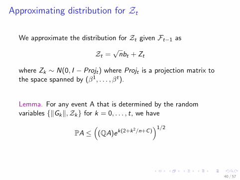
Approximating distribution for Zt
We approximate the distribution for Zt given Ft−1 as
Zt =√nbt + Zt
where Zk ∼ N(0, I − Projt) where Projt is a projection matrix tothe space spanned by (β1, . . . , βt).
Lemma. For any event A that is determined by the randomvariables {∥Gk∥,Zk} for k = 0, . . . , t, we have
PA ≤((QA)ek(2+k2/n+C)
)1/2
40 / 57

.
.
.
.
.
.
.
.
.
.
.
.
.
.
.
.
.
.
.
.
.
.
.
.
.
.
.
.
.
.
.
.
.
.
.
.
.
.
.
.
Combining Components
Class of statistics statt formed by combining Z0, . . . ,Zk :
statt,j = τt Zcombt,j + βt
j , j = 1, . . . ,N
with Zcombt = λ0Z0 + λ1Z1 + . . .+ λt Zt ,
∑k λ
2k = 1
Ideal Distribution of the combined statistics
stat idealk = β + τtZcombk
where τ2t = σ2 + (1− xt)P , and Z combk i.i.d. ∼ N (0, 1)
What choice of λk ’s gives you the ideal ?
41 / 57

.
.
.
.
.
.
.
.
.
.
.
.
.
.
.
.
.
.
.
.
.
.
.
.
.
.
.
.
.
.
.
.
.
.
.
.
.
.
.
.
Oracle statistics
Choosing weights based on (λ0, . . . , λt) proportional to((√
n(σ2 + P)− bT0 βt), −(bT1 β
t), . . . , −(bTt βt)
)Combining Zk with these weights, replacing χn−k with
√n, it
produces the desired distributional representation
statt = τt
t∑k=0
λkZk + βt ≈ β + τtZcombt
with Z combt ∼ N(0, I).
But can’t calculate these weights not knowing β: b0 = β/√P + σ2
42 / 57

.
.
.
.
.
.
.
.
.
.
.
.
.
.
.
.
.
.
.
.
.
.
.
.
.
.
.
.
.
.
.
.
.
.
.
.
.
.
.
.
Oracle weights vs Estimated Weights
Oracle weights of combination: (λ0, . . . , λt) proportional to((√
n(σ2 + P)− bT0 βt), −(bT1 β
t), . . . , −(bTt βt)
)produces statt with the desired representation β + τtZ
combt
Estimated weights of combination: (λ1, . . . , λt) proportional to((∥Y ∥ − ZT
0 βt/√n, −(ZT
1 βt)/√n, . . . , −(ZT
k βt)/√n)
produce the residual-based statistics previously discussed, which wehave seen are not close enough to the desired distribution
43 / 57

.
.
.
.
.
.
.
.
.
.
.
.
.
.
.
.
.
.
.
.
.
.
.
.
.
.
.
.
.
.
.
.
.
.
.
.
.
.
.
.
Orthogonalization Interpretation of Ideal Weights
Estimation of((σY − bT0 β
t), −(bT1 βt), . . . , −(bTt β
t)):
These bTk βt arise in the QR-decomposition for B = [β, β1, . . . , βt ]
B = [b0 b1 . . . bk ]
bT0 β bT0 β1 . . . bT0 β
t
0 bT1 β1 . . . bT1 β
t
......
. . ....
0 0 . . . bTt βt
Noting that b0, . . . , bt are orthonormal, we can express BTB as . . .
44 / 57

.
.
.
.
.
.
.
.
.
.
.
.
.
.
.
.
.
.
.
.
.
.
.
.
.
.
.
.
.
.
.
.
.
.
.
.
.
.
.
.
Cholesky Decomposition of BTB
βTβ βTβ1 . . . βTβt
(β1)Tβ (β1)Tβ1 . . . (β1)Tβt
......
. . ....
(βt)Tβ . . . . . . (βt)Tβt
=RT
bT0 β bT0 β1 . . . bT0 β
t
0 bT1 β1 . . . bT1 β
t
......
. . ....
0 0 . . . bTt βt
Deterministic weights:
• Replace elements on LHS with deterministic values underdesired representation: 1
nE(βk)Tβt = 1
nE(βk)Tβ = xkP for
k ≤ t
• Then perform Cholesky decomposition of LHS to getdeterministic weights
45 / 57

.
.
.
.
.
.
.
.
.
.
.
.
.
.
.
.
.
.
.
.
.
.
.
.
.
.
.
.
.
.
.
.
.
.
.
.
.
.
.
.
Cholesky Decomposition of BTB
With τ2k = σ2 + (1− xk)P:
τ 20 x1P . . . xtP
x1P x1P . . . x1P
......
. . ....
xtP . . . . . . xtP
=RT
τ0 τ0 − τ 21√ω0 . . . σY − τ 2k
√ω0
0 τ 21√ω1 . . . τ 2k
√ω1
......
. . ....
0 0 . . . τ 2t√ωt
In the above, ω0 =
1τ20
and ωk = 1τ2k
− 1τ2k−1
for k ≥ 1
The last column gives the deterministic weights of combination
46 / 57
.
.
.
.
.
.
.
.
.
.
.
.
.
.
.
.
.
.
.
.
.
.
.
.
.
.
.
.
.
.
.
.
.
.
.
.
.
.
.
.
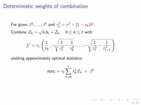
Deterministic weights of combination
For given β1, . . . , βt and τ2k = σ2 + (1− xk)P
Combine Zk =√n bk + Zk , 0 ≤ k ≤ t with
λ∗ = τt
(1
τ0,−
√1
τ21− 1
τ20, . . . ,−
√1
τ2t− 1
τ2t−1
)
yielding approximately optimal statistics
statt = τt
t∑k=0
λ∗kZk + βt
47 / 57
.
.
.
.
.
.
.
.
.
.
.
.
.
.
.
.
.
.
.
.
.
.
.
.
.
.
.
.
.
.
.
.
.
.
.
.
.
.
.
.
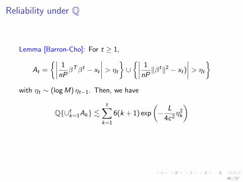
Reliability under Q
Lemma [Barron-Cho]: For t ≥ 1,
At =
{∣∣∣∣ 1nP βTβt − xt
∣∣∣∣ > ηt
}∪{∣∣∣∣ 1nP ∥βt∥2 − xt)
∣∣∣∣ > ηt
}with ηt ∼ (logM) ηt−1. Then, we have
Q{∪tk=1Ak} ≲
t∑k=1
6(k + 1) exp
(− L
4c2η2k
)
48 / 57

.
.
.
.
.
.
.
.
.
.
.
.
.
.
.
.
.
.
.
.
.
.
.
.
.
.
.
.
.
.
.
.
.
.
.
.
.
.
.
.
Update Plots for Deterministic and Oracle Weights
L = 512, M = 64, snr = 15, C = 2 bits, R = 0.7C, n = 2194
Ran 10 trials for each method. We see that they follow theexpected update function.
49 / 57

.
.
.
.
.
.
.
.
.
.
.
.
.
.
.
.
.
.
.
.
.
.
.
.
.
.
.
.
.
.
.
.
.
.
.
.
.
.
.
.
Cholesky decomposition based estimates
βTβ βTβ1 . . . βTβt
(β1)Tβ (β1)Tβ1 . . . (β1)Tβt
......
. . ....
(βt)Tβ . . . . . . (βt)Tβt
=RT
bT0 β bT0 β1 . . . bT0 β
t
0 bT1 β1 . . . bT1 β
t
......
. . ....
0 0 . . . bTt βt
Another Idea: Instead of replacing entire LHS with deterministicvalues, retain the entries we already know . . .
50 / 57

.
.
.
.
.
.
.
.
.
.
.
.
.
.
.
.
.
.
.
.
.
.
.
.
.
.
.
.
.
.
.
.
.
.
.
.
.
.
.
.
Cholesky Decomposition-based Estimated Weights
βTβ βTβ1 . . . βTβt
(β1)Tβ (β1)Tβ1 . . . (β1)Tβt
......
. . ....
(βt)Tβ . . . . . . (βt)Tβt
=RT
bT0 β bT0 β1 . . . bT0 β
t
0 bT1 β1 . . . bT1 β
t
......
. . ....
0 0 . . . bTt βt
Under Q, we haveZTk βk
√n
= (bTk βk)
Based on the estimates we can recover the rest of the componentsof the matrix, which leads us to oracle weights under theapproximating distribution, which we denote λt .
51 / 57

.
.
.
.
.
.
.
.
.
.
.
.
.
.
.
.
.
.
.
.
.
.
.
.
.
.
.
.
.
.
.
.
.
.
.
.
.
.
.
.
Cholesky weights of combination
Combine Z0, . . . ,Zt with weights λt :
statt = τt
t∑k=0
λkZk + βt
where τt2 = σ2 + ∥β − βt∥2, to get desired distributional
representation under Q:
statt ≈ β + τtZcombk
52 / 57

.
.
.
.
.
.
.
.
.
.
.
.
.
.
.
.
.
.
.
.
.
.
.
.
.
.
.
.
.
.
.
.
.
.
.
.
.
.
.
.
Reliability under Q
Lemma [Barron-Cho]: Suppose we have a Lipschitz condition onthe update function with cLip ≤ 1 so that
|g(x1)− g(x2)| ≤ cLip|x1 − x2|.
For t ≥ 1,
At =
{∣∣∣∣ 1nP βTβt − xt
∣∣∣∣ > tη
}∪{∣∣∣∣ 1nP ∥βt∥2 − xt
∣∣∣∣ > tη
}Then, we have
Q{∪tk=1Ak} ≲ exp
(− L
8c2η2)
53 / 57

.
.
.
.
.
.
.
.
.
.
.
.
.
.
.
.
.
.
.
.
.
.
.
.
.
.
.
.
.
.
.
.
.
.
.
.
.
.
.
.
Update Plots for Cholesky-based Weights
L = 512, M = 64, snr = 7, C = 1.5 bits, R = 0.7C, n = 2926
0.0 0.2 0.4 0.6 0.8 1.0
0.0
0.2
0.4
0.6
0.8
1.0
Update Function
x(k)
x(k+1)
CholeskyOracle
Red (cholesky decomposition based weights); green (oracle weightsof combination). Ran 10 trials for each.
54 / 57

.
.
.
.
.
.
.
.
.
.
.
.
.
.
.
.
.
.
.
.
.
.
.
.
.
.
.
.
.
.
.
.
.
.
.
.
.
.
.
.
Improving the End Game• Variable power: Pℓ proportional to e−2Cℓ/L for ℓ = 1, . . . , L• When R is not close to C, say R = 0.6C, this allocates toomuch power to initial sections, leaving too little for the end
• We use alternative power allocation: constant leveling thepower allocation for the last portion of the sections
L = 512, snr = 7, C = 1.5 bits
55 / 57

.
.
.
.
.
.
.
.
.
.
.
.
.
.
.
.
.
.
.
.
.
.
.
.
.
.
.
.
.
.
.
.
.
.
.
.
.
.
.
.
Progression Plot using Alternative Power Allocation
L = 512, M = 64, snr = 7, C = 1.5 bits, R = 0.7C, n = 2926.
0.0 0.2 0.4 0.6 0.8 1.0
0.0
0.2
0.4
0.6
0.8
1.0
L=512,M=64, n=2926, rate=0.73 snr=7 at step12
u_l
w_j_l
stripeno-stripe
Progression plot of the final step. The area under the curve mightbe the same, the expected weights for the last sections are higherwhen we level the power at the end
56 / 57

.
.
.
.
.
.
.
.
.
.
.
.
.
.
.
.
.
.
.
.
.
.
.
.
.
.
.
.
.
.
.
.
.
.
.
.
.
.
.
.
Summary
Sparse superposition codes with adaptive successive decoding
• Simplicity of the code permits:• distributional analysis of the decoding progression• low complexity decoder• exponentially small error probability for any fixed R < C
• Asymptotics superior to polar code bounds for such rates
Next . . .
• Approximate message passing (AMP) decoding
• Power-allocation schemes to improve finite block-lengthperformance
57 / 57