HAL Id: hal-00362471https://hal.archives-ouvertes.fr/hal-00362471v4

Submitted on 15 Feb 2010

HAL is a multi-disciplinary open accessarchive for the deposit and dissemination of sci-entific research documents, whether they are pub-lished or not. The documents may come fromteaching and research institutions in France orabroad, or from public or private research centers.

L’archive ouverte pluridisciplinaire HAL, estdestinée au dépôt et à la diffusion de documentsscientifiques de niveau recherche, publiés ou non,émanant des établissements d’enseignement et derecherche français ou étrangers, des laboratoirespublics ou privés.

Sparse Regression Learning by Aggregation andLangevin Monte-Carlo

Arnak S. Dalalyan, Alexandre Tsybakov

To cite this version:Arnak S. Dalalyan, Alexandre Tsybakov. Sparse Regression Learning by Aggregation and LangevinMonte-Carlo. Journal of Computer and System Sciences, Elsevier, 2012, 78, pp.1423-1443.<10.1016/j.jcss.2011.12.023>. <hal-00362471v4>

Sparse Regression Learning by Aggregation and Langevin Monte-Carlo

A.S. Dalalyana, A.B. Tsybakovb

aIMAGINE, LIGM, Universite Paris Est, Ecole des Ponts ParisTech, FRANCEbCREST and LPMA, Universite Paris 6,FRANCE

Abstract

We consider the problem of regression learning for deterministic design and independent random errors.We start by proving a sharp PAC-Bayesian type bound for the exponentially weighted aggregate (EWA)under the expected squared empirical loss. For a broad classof noise distributions the presented boundis valid whenever the temperature parameterβ of the EWA is larger than or equal to 4σ2, whereσ2 is thenoise variance. A remarkable feature of this result is that it is valid even for unbounded regression functionsand the choice of the temperature parameter depends exclusively on the noise level.

Next, we apply this general bound to the problem of aggregating the elements of a finite-dimensionallinear space spanned by a dictionary of functionsφ1, . . . , φM. We allow M to be much larger than thesample sizen but we assume that the true regression function can be well approximated by a sparse linearcombination of functionsφ j . Under this sparsity scenario, we propose an EWA with a heavytailed priorand we show that it satisfies a sparsity oracle inequality with leading constant one.

Finally, we propose several Langevin Monte-Carlo algorithms to approximately compute such an EWAwhen the numberM of aggregated functions can be large. We discuss in some detail the convergence ofthese algorithms and present numerical experiments that confirm our theoretical findings.

Keywords: Sparse learning, regression estimation, logistic regression, oracle inequalities, sparsity prior,Langevin Monte-Carlo.

1. Introduction

In recent years a great deal of attention has been devoted to learning in high-dimensional models underthe sparsity scenario. This typically assumes that, in addition to the sample, we have a finite dictionary ofvery large cardinality such that a small set of its elements provides a nearly complete description of theunderlying model. Here, the words “large” and “small” are understood in comparison with the sample size.Sparse learning methods have been successfully applied in bioinformatics, financial engineering, imageprocessing, etc. (see, e.g., the survey in [44]).

A popular model in this context is linear regression. We observe n pairs (X1,Y1), . . . , (Xn,Yn), whereeachXi – called the predictor – belongs toRM andYi – called the response – is scalar and satisfiesYi =

X⊤i λ0+ ξi with some zero-mean noiseξi . The goal is to develop inference on the unknown vectorλ0 ∈ RM.In many applications of linear regression the dimension ofXi is much larger than the sample size, i.e.,

M ≫ n. It is well-known that in this case classical procedures, such as the least squares estimator, do notwork. One of the most compelling ways for dealing with the situation whereM ≫ n is to suppose that thesparsity assumption is fulfilled, i.e., thatλ0 has only few coordinates different from 0. This assumption ishelpful at least for two reasons: The model becomes easier tointerpret and the consistent estimation ofλ0

becomes possible if the number of non-zero coordinates is small enough.During the last decade several learning methods exploitingthe sparsity assumption have been discussed

in the literature. Theℓ1-penalized least squares (Lasso) is by far the most studied one and its statisticalproperties are now well understood (cf., e.g., [4, 6, 7, 5, 31, 39, 45] and the references cited therein). TheLasso is particularly attractive by its low computational cost. For instance, one can use the LARS algo-rithm [19], which is quite popular. Other procedures based on closely related ideas include the Elastic Net

Email addresses:dalalyan@imagine.enpc.fr (A.S. Dalalyan),alexandre.tsybakov@ensae.fr (A.B. Tsybakov)

Preprint submitted to JCSS February 16, 2010

[47], the Dantzig selector [9] and the least squares with entropy penalization [27]. However, one impor-tant limitation of these procedures is that they are provably consistent under rather restrictive assumptionson the Gram matrix associated to the predictors, such as the mutual coherence assumption [18], the uni-form uncertainty principle [8], the irrepresentable [46] or the restricted eigenvalue [4] conditions. This issomewhat unsatisfactory, since it is known that, at least intheory, there exist estimators attaining optimalaccuracy of prediction under almost no assumption on the Gram matrix. This is, in particular, the case forthe ℓ0-penalized least squares estimator [7, Thm. 3.1]. However,the computation of this estimator is anNP-hard problem. We finally mention the paper [42], which brings to attention the fact that the empiricalBayes estimator in Gaussian regression with Gaussian priorcan effectively recover the sparsity pattern.This method is realized in [42] via the EM algorithm. However, its theoretical properties are not explored,and it is not clear what are the limits of application of the method beyond the considered set of numericalexamples.

In [15, 16] we proposed another approach to learning under the sparsity scenario, which consists inusing an exponentially weighted aggregate (EWA) with a properly chosen sparsity-favoring prior. Thereexists an extensive literature on EWA. Some recent results focusing on the statistical properties can be foundin [2, 3, 11, 24, 28, 43]. Application of EWA to the single-index regression and Gaussian graphical modelshas been developed in [20] and [21], respectively. Procedures with exponential weighting received muchattention in the literature on the on-line learning, see [12, 22, 40], the monograph [14] and the referencescited therein.

The main message of [15, 16] is that the EWA with a properly chosen prior is able to deal with thesparsity issue. In particular, [15, 16] prove that such an EWA satisfies a sparsity oracle inequality (SOI),which is more powerful than the best known SOI for other common procedures of sparse recovery. Animportant point is that almost no assumption on the Gram matrix is required. In the present work weextend this analysis in two directions. First, we prove a sharp PAC-Bayesian bound for a large class ofnoise distributions, which is valid for the temperature parameter depending only on the noise distribution.We impose no restriction on the values of the regression function. This result is presented in Section 2. Theconsequences in the context of linear regression under sparsity assumption are discussed in Section 3.

The second problem that we analyze here is the computation ofEWA with the sparsity prior. Sincewe want to deal with large dimensionsM, computation of integrals overRM in the definition of this esti-mator can be a hard problem. Therefore, we suggest an approximation based on Langevin Monte-Carlo(LMC). This is described in detail in Section 4. Section 5 contains numerical experiments that confirm fastconvergence properties of the LMC and demonstrate a nice performance of the resulting estimators.

2. PAC-Bayesian type oracle inequality

Throughout this section, as well as in Section 3, we assume that we are given the data (Zi ,Yi), i =1, . . . , n, generated by the non-parametric regression model

Yi = f (Zi) + ξi , i = 1, . . . , n, (1)

with deterministic designZ1, . . . ,Zn and random errorsξi . We use the vector notationY = f + ξ, whereξ = (ξ1, . . . , ξn)⊤ and the functionf (·) is identified with the vectorf = ( f (Z1), . . . , f (Zn))⊤. The spaceZ containing the design pointsZi can be arbitrary andf is a mapping fromZ to R. For each functionh : Z → R, we denote by‖h‖n the empirical norm

(1n

∑ni=1 h(Zi)2)1/2. Along with these notation, we

will denote by‖v‖p the ℓp-norm of a vectorv = (v1, . . . , vn) ∈ Rn, that is‖v‖pp =

∑ni=1 |vi |p, 1 6 p < ∞,

‖v‖∞ = maxi |vi | and‖v‖0 is the number of nonzero entries ofv. With this notation,‖ f ‖22 = n‖ f ‖2n.Assume that we are given a collection{ fλ : λ ∈ Λ} of functions fλ : Z → R that will serve as building

blocks for the learning procedure.The setΛ is assumed to be equipped with aσ-algebra and the mappingsλ 7→ fλ(z) are assumed to be measurable with respect to thisσ-algebra for allz ∈ Z. Letπ be a probabilitymeasure onΛ, called the prior, and letβ be a positive real number, called the temperature parameter. Wedefine the EWA by

fn(z) =∫

Λ

fλ(z) πn,β(dλ),

2

whereπn,β is the (posterior) probability distribution

πn,β(dλ) ∝ exp{ − β−1‖Y − f λ‖22

}π(dλ),

and f λ = ( fλ(Z1), . . . , fλ(Zn))⊤. We denote byL the smallest positive number, which may be equal to+∞,such that

(λ, λ′) ∈ Λ2=⇒ max

i| fλ(Zi) − fλ′ (Zi)| 6 L (2)

In the sequel, we use the convention+∞+∞ = 0 and, for any functionv : R → R, we denote by‖v‖∞ its

L∞(R)-norm.In order to get meaningful statistical results on the accuracy of the EWA, some conditions on the noise

are imposed. In addition to the standard assumptions that the noise vectorξ = (ξ1, . . . , ξn)⊤ has zeromean and independent identically distributed (iid) coordinates, we require the following assumption on thedistribution ofξ1.

Assumption N. For anyγ > 0 small enough, there exist a probability space and two random variablesξandζ defined on this probability space such that

i) ξ has the same distribution as the regression errorsξi ,ii) ξ + ζ has the same distribution as (1+ γ)ξ and the conditional expectation satisfiesE[ζ | ξ] = 0,iii) there existt0 ∈ (0,∞] and a bounded Borel functionv : R→ R+ such that

limγ→0

sup(t,a)∈[−t0,t0]×supp(ξ)

logE[etζ | ξ = a]t2γv(a)

6 1,

where supp(ξ) is the support of the distribution ofξ.

Many symmetric distributions used in applications satisfyAssumption N with functionsv such that‖v‖∞is a multiple of the variance of the noiseξi . This follows from Remarks 1-6 given at the end of this sectionand their combinations.

Theorem 1. Let Assumption N be satisfied with some function v and let (2) hold. Then for any priorπ, anyprobability measure p onΛ and anyβ > max(4‖v‖∞, 2L/t0) we have

E[‖ fn − f ‖2n] 6∫

Λ

‖ f − fλ‖2n p(dλ) +βK(p, π)

n,

whereK(· , · ) stands for the Kullback-Leibler divergence.

Prior to presenting the proof, let us note that Theorem 1 is inthe spirit of [16, Theorems 1,2], but isbetter in several aspects. First, the main assumption ensuring the validity of the oracle inequality involvesthe distribution of the noise alone, while [16, Theorem 2] relies on an assumption (denoted by(C) in [16])that ties together the distributional properties of the noise and the nature of the dictionary{ fλ}. A secondadvantage is that Assumption N is independent of the sample size n and, consequently, suggests a choiceof the parameterβ that does not change with the sample size. Theorem 1 of [16] also has these advantagesbut it is valid only for a very restricted class of noise distributions, essentially for the Gaussian and uniformnoise. As we shall see later in this section, Theorem 1 leads to a choice of the tuning parameterβ, which isvery simple and guarantees the validity of a strong oracle inequality for a large class of noise distributions.

Proof of Theorem 1.It suffices to prove the theorem forp such that∫Λ‖ fλ − f ‖2n p(dλ) < ∞ and p ≪ π

(implyingK(p, π) < ∞), since otherwise the result is trivial.We first assume thatβ > 4‖v‖∞ and thatL < ∞. Letγ > 0 be a small number. Let now (ξ1, ζ1), . . . , (ξn, ζn)

be a sequence of iid pairs of random variables defined on a common probability space such that (ξi , ζi) sat-isfy conditions i)-iii) of Assumption N for anyi. The existence of these random variables is ensured byAssumption N. We use here the same notationξi as in model (1), since it causes no ambiguity.

Set hλ = fλ − f , h = fn − f , ζ = (ζ1, . . . , ζn)⊤, U(h, h′) = ‖h‖22 + 2h⊤h′ and∆U(h, h′, h′′) =(‖h‖22 − ‖h

′‖22) + 2(h − h′)⊤h′′ for any pairh, h′, h′′ ∈ Rn. With this notation we have

E[‖ fn − f ‖2n] = E[‖h‖2n] = E[‖h‖2n +

2nγ

h⊤ζ].

3

Therefore,E[‖ fn − f ‖2n] = S + S1, where

S = − βnγ

E[log

∫

Λ

exp(− γU(hλ, γ−1ζ)

β

)πn,β(dλ)

],

S1=β

nγE[log

∫

Λ

exp(− γ∆U(hλ, h, γ−1ζ)

β

)πn,β(dλ)

].

We first bound the termS. To this end, note that

πn,β(dλ) =exp{−β−1U(hλ, ξ)}∫

Λexp{−β−1U(hw, ξ)}π(dw)

π(dλ)

and, therefore,

S =β

nγE[log

∫

Λ

exp{− 1

βU(hλ, ξ)

}π(dλ)

]− β

nγE[log

∫

Λ

exp{ − 1+γ

βU

(hλ,

ξ+ζ

1+γ

)}π(dλ)

].

By part ii) of Assumption N and the independence of vectors (ξi , ζi) for different values ofi, the probabilitydistribution of the vector (ξ+ζ)/(1+γ) coincides with that ofξ. Therefore, (ξ+ζ)/(1+γ) may be replacedby ξ inside the second expectation. Now, using the Holder inequality, we get

S 6 − β

n(1+ γ)E[log

∫

Λ

e−(1+γ)β−1U(hλ,ξ)π(dλ)].

Next, by a convex duality argument [10, p. 160], we find

S 6

∫

Λ

‖hλ‖2n p(dλ) +βK(p, π)n(1+ γ)

.

Let us now bound the termS1. According to part iii) of Assumption N, there existsγ0 > 0 such that∀γ 6 γ0,

sup|t|6t0

logE[etζ |ξ = a]t2γ

6 v(a)(1+ oγ(1)), ∀ a ∈ R.

In what follows we assume thatγ 6 γ0. Since for everyi, |2β−1(hλ(Zi) − h(Zi))| 6 2β−1L 6 t0, usingJensen’s inequality we get

S1 6β

nγE[log

∫

Λ

exp{− nγ

β(‖hλ‖2n − ‖h‖2n)

}θλ E

(exp

{ n∑

i=1

2β−1(hλ(Zi) − h(Zi))ζi

}∣∣∣ξ)π(dλ)

]

6β

nγE[log

∫

Λ

exp{− nγ

β(‖hλ‖2n − ‖h‖2n)

}θλ exp

{4n‖v‖∞γβ2

‖hλ − h‖2n(1+ oγ(1))}π(dλ)

].

For γ small enough (γ 6 γ0), this entails that up to a positive multiplicative constant, the termS1 is

bounded by the expressionE[log

∫Λ

exp( − nγV(hλ ,h)

β2

)θλπ(dλ)

], where

V(hλ, h)= β(‖hλ‖2n − ‖h‖2n)+(β + 4‖v‖∞)

2‖hλ− h‖2n.

Using [15, Lemma 3] and Jensen’s inequality we obtainS1 6 0 for anyγ 6 (β − 4‖v‖∞)/4nL. Thus, weproved that

E[‖h‖2n] 6∫

Λ

‖hλ‖2n p (dλ) +βK(p, π)n(1+ γ)

for anyγ 6 γ0 ∧ (β − 4‖v‖∞)/4nL. Lettingγ tend to zero, we obtain

E[‖h‖2n] 6∫

Λ

‖hλ‖2np(dλ) +βK(p, π)

n

4

for any β > max(4‖v‖∞, 2L/t0). Fatou’s lemma allows us to extend this inequality to the case β =max(4‖v‖∞, 2L/t0).

To cover the caseL = +∞, t0 = +∞, we fix someL0 ∈ (0,∞) and apply the obtained inequality to thetruncated priorπL′ (dλ) ∝ 1lΛL′ (λ)π(dλ), whereL′ ∈ (L0,∞) andΛL′ = {λ ∈ Λ : maxi | fλ(Zi)| 6 L′}. Weobtain that for any measurep≪ π supported byΛL0,

E[‖hL′‖2n] 6∫

Λ

‖hλ‖2n p(dλ) +βK(p, πL′ )

n

6

∫

Λ

‖hλ‖2n p(dλ) +βK(p, π)

n.

One easily checks thathL′ tends a.s. toh and that the random variable supL′>L0‖hL′‖2n1l(maxi |ξi | 6 C) is

integrable for any fixedC. Therefore, by Lebesgue’s dominated convergence theorem we get

E[‖h‖2n1l(maxi|ξi | 6 C)] 6

∫

Λ

‖hλ‖2n p(dλ) +βK(p, π)

n.

Letting C tend to infinity and using Lebesgue’s monotone convergence theorem we obtain the desiredinequality for any probability measurep which is absolutely continuous w.r.t.π and is supported byΛL0

for someL0 > 0. If p(ΛL0) < 1 for anyL0 > 0, one can replacep by its truncated versionpL′ and useLebesgue’s monotone convergence theorem to get the desiredresult.

The following remarks provide examples of noise distributions, for which Assumption N is satisfied.Proofs of these remarks are given in the Appendix.

Remark 1 (Gaussian noise). If ξ1 is drawn according to the Gaussian distributionN(0, σ2), then for anyγ > 0 one can chooseζ independently ofξ according to the Gaussian distributionN(0, (2γ + γ2)σ2). Thisresults in v(a) ≡ σ2 and, as a consequence, Theorem 1 holds for anyβ > 4σ2. Note that this reduces tothe Leung and Barron’s [28] result if the priorπ is discrete.

Remark 2 (Rademacher noise). If ξ1 is drawn according to the Rademacher distribution, i.e.P(ξ1 = ±σ) =1/2, then for anyγ > 0 one can defineζ as follows:

ζ = (1+ γ)σ sgn[σ−1ξ − (1+ γ)U] − ξ,

where U is distributed uniformly in[−1, 1] and is independent ofξ. This results in v(a) ≡ σ2 and, as aconsequence, Theorem 1 holds for anyβ > 4σ2

= 4E[ξ21].

Remark 3 (Stability by convolution). Assume thatξ1 andξ′1 are two independent random variables. Ifξ1

andξ′1 satisfy Assumption N with t0 = ∞ and with functions v(a) and v′(a), then any linear combinationαξ1 + α

′ξ′1 satisfies Assumption N with t0 = ∞ and the v-functionα2v(a) + (α′)2v′(a).

Remark 4 (Uniform distribution). The claim of preceding remark can be generalized to linear combi-nations of a countable set of random variables, provided that the series converges in the mean squaredsense. In particular, ifξ1 is drawn according to the symmetric uniform distribution with varianceσ2, thenAssumption N is fulfilled with t0 = ∞ and v(a) ≡ σ2. This can be proved using the fact thatξ1 has thesame distribution asσ

∑∞i=1 2−iηi , whereηi are iid Rademacher random variables. Thus, in this case the

inequality of Theorem 1 is true for anyβ > 4σ2.

Remark 5 (Laplace noise). If ξ1 is drawn according to the Laplace distribution with varianceσ2, then foranyγ > 0 one can chooseζ independently ofξ according to the distribution associated to the characteristicfunction

ϕ(t) =1

(1+ γ)2

(1+

2γ + γ2

1+ (1+ γ)2(σt)2/2

).

One can observe that the distribution ofζ is a mixture of the Dirac distribution at zero and the Laplacedistribution with variance(1 + γ)2σ2. This results in v(a) ≡ 2σ2/(2 − σ2t20) and, as a consequence, bytaking t0 = 1/σ2, we get that Theorem 1 holds for anyβ > max(8σ2, 2Lσ).

5

Remark 6 (Bounded symmetric noise). Assume that the errorsξi are symmetric and that P(|ξi | 6 B) = 1for some B∈ (0,∞). Let U ∼ U([−1, 1]) be a random variable independent ofξ. Then,ζ = (1 +γ)|ξ| sgn[sgn(ξ) − (1 + γ)U] − ξ satisfies Assumption N with v(a) = a2. Since‖v‖∞ 6 B2, we obtain thatTheorem 1 is valid for anyβ > 4B2.

Consider now the case of finiteΛ. W.l.o.g. we suppose thatΛ = {1, . . . ,M}, { fλ, λ ∈ Λ} = { f1, . . . , fM}and we take the uniform priorπ(λ = j) = 1/M. From Theorem 1 we immediately get the following sharporacle inequality for model selection type aggregation.

Corollary 1. Let Assumption N be satisfied with some function v and let (2) hold. Then for the uniformprior π(λ = j) = 1/M, j = 1, . . . ,M, and anyβ > max(4‖v‖∞, 2L/t0) we have

E[‖ fn − f ‖2n] 6 minj=1,...,M

‖ f j − f ‖2n +β log M

n.

This corollary can be compared with bounds for combining procedures in the theory of prediction ofdeterministic sequences [41, 29, 13, 26, 12, 14]. With our notation, the bounds proved in these works canbe written is the form

1n

n∑

i=1

(Yi − f ∗(Zi))26 C1 min

j=1,...,M

1n

n∑

i=1

(Yi − f j(Zi))2+

C2 log Mn

. (3)

Here f j(Zi) is interpreted as the value ofYi predicted by thejth procedure,f ∗(Zi) as an aggregated forecast,and C1 > 1, C2 > 0 are constants. Such inequalities are proved under the assumption thatYi ’s aredeterministic and uniformly bounded. WhenC1 = 1, applying (3) to random uniformly boundedYi ’sfrom model (1) withE(ξi) = 0 and taking expectations can yield an oracle inequality similar to that ofCorollary 1. However, the uniform boundedness ofYi ’s supposes that not only the noiseξi but also thefunctionsf and f j are uniformly bounded. Bounds onf should be a priori known for the construction of theaggregated rulef ∗ in (3) but in practice they are not always available. Our results are free of this drawbackbecause they hold with no assumption onf . We have no assumption on the dictionary{ f1, . . . , fM} neither.

3. Sparsity prior and SOI

In this section we introduce the sparsity prior and present asparsity oracle inequality (SOI) derivedfrom Theorem 1.

In what follows we assume thatΛ ⊂ RM for some positive integerM. We will use boldface letters to

denote vectors and, in particular, the elements ofΛ. For any square matrixA, let Tr(A) denote the trace(sum of diagonal entries) ofA. Furthermore, we focus on the particular case whereFΛ is the image ofa convex polytope inRM by a link function g : R → R. More specifically, we assume that, for someR ∈ (0,+∞] and for a finite number of measurable functions

{φ j

}j=1,...,M,

FΛ ={

fλ(z) = g( M∑

j=1

λjφ j(z)), ∀z ∈ Z

∣∣∣∣ λ ∈ RM satisfies‖λ‖1 6 R

},

where‖λ‖1 =∑

j |λj | stands for theℓ1-norm. The link functiong is assumed twice continuously differen-tiable and known. Typical examples of link function includethe linear functiong(x) = x, the exponentialfunction g(x) = ex, the logistic functiong(x) = ex/(ex

+ 1), the cumulative distribution function of thestandard Gaussian distribution, and so on.

If, in addition, f ∈ FΛ, then model (1) reduces to that of single-index regression with known linkfunction. In the particular case ofg(x) = x, this leads to the linear regression defined in the Introduction.Indeed, it suffices to take

Xi = (φ1(Zi), . . . , φM(Zi))⊤, i = 1, . . . , n.

This notation will be used in the rest of the paper along with the assumption thatXi are normalized so thatall the diagonal entries of matrix1n

∑ni=1 Xi X⊤i are equal to one.

6

Figure 1: The boxplots of a sample of size 104 drawn from the scaled Gaussian, Laplace and Studentt(3) distributions. In all thethree cases the location parameter is 0 and the scale parameter is 10−2.

The familyFΛ defined above satisfies inequality (2) withL = 2R‖g′‖∞Lφ, whereLφ = maxi, j |φ j(Zi)|and‖g′‖∞ is the maximum of the derivative ofg on the interval [−RLφ,RLφ]. Indeed, sinceΛ is theℓ1 ball ofradiusR in R

M andφ js are bounded byLφ, the real numbersui = λ⊤Xi andu′i = λ

′⊤Xi belong to the interval

[−RLφ,RLφ] for everyλ andλ′ from Λ. Consequently,| fλ(Zi) − fλ′ (Zi)| = |g(ui) − g(u′i )| =∫ u′i

uig′(s) ds is

bounded by‖g′‖∞|ui − u′i |, the latter being smaller than 2R‖g′‖∞Lφ.We allow M to be large, possibly much larger than the sample sizen. If M ≫ n, we have in mind that

the sparsity assumption holds, i.e., there existsλ∗ ∈ RM such thatf in (1) is close tofλ∗ for someλ∗ havingonly a small number of non-zero entries. We handle this situation via a suitable choice of priorπ. Namely,we use a modification of the sparsity prior proposed in [15]. It should be emphasized right away that wewill take advantage of sparsity for the purpose of prediction and not for data compression. In fact, even ifthe underlying model is sparse, we do not claim that our estimator is sparse as well, but we claim that it isquite accurate under very mild assumptions. On the other hand, some numerical experiments demonstratethe sparsity of our estimator and the fact that it recovers correctly the true sparsity pattern in exampleswhere the (restrictive) assumptions mentioned in the Introduction are satisfied (cf. Section 5). However,our theoretical results do not deal with this property.

To specify the sparsity priorπ we need the Huber function ¯ω : R→ R defined by

ω(t) =

t2, if |t| 6 1

2|t| − 1, otherwise.

This function behaves very much like the absolute value oft, but has the advantage of being differentiableat every pointt ∈ R. Let τ andα be positive numbers. We define thesparsity prior

π(dλ) =τ2M

Cα,τ,R

{ M∏

j=1

e−ω(αλj )

(τ2 + λ2j )2

}1l(‖λ‖1 6 R) dλ, (4)

whereCα,τ,R is the normalizing constant.Since the sparsity prior (4) looks somewhat complicated, anheuristical explanation is in order. Let us

assume thatR is large andα is small so that the functionse−ω(αλj ) and 1l(‖λ‖1 6 R) are approximately equalto one. With this in mind, we can notice thatπ is close to the distribution of

√2τY, whereY is a random

vector having iid coordinates drawn from Student’s t-distribution with three degrees of freedom. In theexamples below we choose a very smallτ, smaller than 1/n. Therefore, most of the coordinates ofτY arevery close to zero. On the other hand, since Student’s t-distribution has heavy tails, a few coordinates ofτY are quite far from zero.

These heuristics are illustrated by Figure 1 presenting theboxplots of one realization of a random vectorin R

10.000 with iid coordinates drawn from the scaled Gaussian, Laplace (double exponential) and Studentt(3) distributions. The scaling factor is such that the probability densities of the simulated distributions areequal to 100 at the origin. The boxplot which is most likely torepresent a sparse vector corresponds toStudent’st(3) distribution.

The relevance of heavy tailed priors for dealing with sparsity has been emphasized by several authors(see [37, Section 2.1] and references therein). However, most of this work focused on logarithmically

7

concave priors, such as the multivariate Laplace distribution. Also in wavelet estimation on classes of“sparse” functions [23] and [33] invoke quasi-Cauchy and Pareto priors. Bayes estimators with heavy-tailed priors in sparse Gaussian shift models are discussedin [1].

The next theorem provides a SOI for the EWA with the sparsity prior (4).

Theorem 2. Let Assumption N be satisfied with some function v and let (2) hold. Take the priorπ definedin (4) andβ > max(4‖v‖∞, 2L/t0). Assume that R> 2Mτ andα 6 1/(4Mτ). Then for allλ∗ such that‖λ∗‖1 6 R− 2Mτ we have

E[‖ fn − f ‖2n] 6 ‖ fλ∗ − f ‖2n +4βn

M∑

j=1

log(1+

|λ∗j |τ

)+

2β(α‖λ∗‖1 + 1)n

+ 4eCg, f τ2M

with Cg, f = 1 if g(x) = x and Cg, f = ‖g′‖2∞ + ‖g′′‖∞(‖g‖∞ + ‖ f ‖∞) for other link functions g.

Proof. Let us define the probability measurep0 by

dp0

dλ(λ) ∝

(dπdλ

(λ − λ∗))1lB1(2Mτ)(λ − λ∗). (5)

Since‖λ∗‖1 6 R− 2Mτ, the conditionλ − λ∗ ∈ B1(2Mτ) implies thatλ ∈ B1(R) and, therefore,p0 isabsolutely continuous w.r.t. the sparsity priorπ. In view of Thm. 1, we have

E[‖ fn − f ‖2n] 6∫

Λ

‖ fλ − f ‖2n p0(dλ) +βK(p0, π)

n.

Since fλ(Zi) = g(X⊤i λ) we have∇λ[( fλ(Zi) − f (Zi))2] = 2g′(X⊤i λ)( fλ(Zi) − f (Zi))Xi and

∇2λ[( fλ(Zi) − f (Zi))2] = 2

{g′(X⊤i λ)

2+ g′′(X⊤i λ)

(g(X⊤i λ) − f (Zi)

)}Xi X⊤i .

One can remark that the factor ofXi X⊤i in the last display is bounded byCg, f . Therefore, in view of theTaylor formula,

( fλ(Zi) − f (Zi))26 ( fλ∗(Zi) − f (Zi))2

+ 2( fλ∗ (Zi) − f (Zi))g′(X⊤i λ∗)X⊤i (λ − λ∗)

+Cg, f [X⊤i (λ − λ∗)]2.

By the symmetry ofp0 with respect toλ∗, the integral∫

(λ − λ∗)p0(dλ) vanishes. Combining this with thefact that the diagonal entries of the matrix1

n

∑i Xi X⊤i are equal to one, we obtain

∫

Λ

‖ fλ − f ‖2n p0(dλ) 6 ‖ fλ∗ − f ‖2n +Cg, f

∫

RM‖λ − λ∗‖22 p0(dλ).

To complete the proof, we use the following technical result.

Lemma 3. For every integer M larger than1, we have:

∫

RM(λ1 − λ∗1)2p0(dλ) 6 4τ2e4Mατ, K(p0, π) 6 2(α‖λ∗‖1 + 1)+ 4

M∑

j=1

log(1+ |λ∗j |/τ).

The proof of this lemma is postponed to the appendix. It is obvious that inequality (5) follows fromLemma 3, since

∫RM ‖λ−λ∗‖22 p0(dλ) = M

∫RM (λ1−λ∗1)2 p0(dλ) and, under the assumptions of the theorem,

e4Mατ 6 e.

Theorem 2 can be used to choose the tuning parametersτ, α,R whenM ≫ n. The idea is to choosethem such that both terms in the second line of (5) were of the order O(1/n). This can be achieved,for example, by takingτ2 ∼ (Mn)−1 andR = O(Mτ). Then the term4β

n

∑Mj=1 log(1 + |λ∗j |/τ) becomes

dominating. It is important that the numberM∗ of nonzero summands in this term is equal to the numberof nonzero coordinates ofλ∗. Therefore, for sparse vectorsλ∗, this term is rather small, namely of the order

8

M∗(log M)/n, which is the same rate as achieved by other methods of sparserecovery, cf. [6, 9, 7, 4]. Animportant difference compared with these and other papers onℓ1-based sparse recovery is that in Theorem2, we have no assumption on the dictionary{φ1, . . . , φM}.

Note that in the case of logistic regression the link function g, as well as its first two derivatives, arebounded by one. Therefore, since the logistic model is mainly used for estimating functionsf with valuesin [0, 1], Theorem 2 holds in this case withCg, f 6 3. Similarly, for the probit model (i.e., when the linkfunctiong is the cdf of the standard Gaussian distribution) andf with values in [0, 1], one easily checksthatCg, f 6 (π−1

+ 1)/2.

4. Computation of the EW-aggregate by the Langevin Monte-Carlo

In this section we suggest Langevin Monte-Carlo (LMC) procedures to approximately compute theEWA with the sparsity prior whenM ≫ n.

4.1. Langevin Diffusion in continuous time

We start by describing a continuous-time Markov process, called the Langevin diffusion, that will playthe key role in this section. LetV : RM → R be a smooth function, which in what follows will be referredto as potential. We will assume that the gradient ofV is locally Lipschitz and is at most of linear growth.This ensures that the stochastic differential equation (SDE)

dLt = ∇V(Lt) dt+√

2dWt, L0 = λ0, t > 0 (6)

has a unique strong solution, called the Langevin diffusion. In the last display,W stands for anM-dimensional Brownian motion andλ0 is an arbitrary deterministic vector fromRM. It is well known thatthe process{Lt}t>0 is a homogeneous Markov process and a semimartingale, cf. [36, Thm. 12.1].

As a Markov process,L may be transient, null recurrent or positively recurrent. The latter case, whichis the most important for us, corresponds to the process satisfying the law of large numbers and implies theexistence of a stationary distribution. In other terms, ifL is positively recurrent, there exists a probabilitydistributionPV onR

M such that the processL is stationary provided that the initial conditionλ0 is drawnat random accordingPV. A remarkable property of the Langevin diffusion—making it very attractive forcomputing high-dimensional integrals—is that its stationary distribution, if exists, has the density

pV(λ) ∝ eV(λ), λ ∈ RM ,

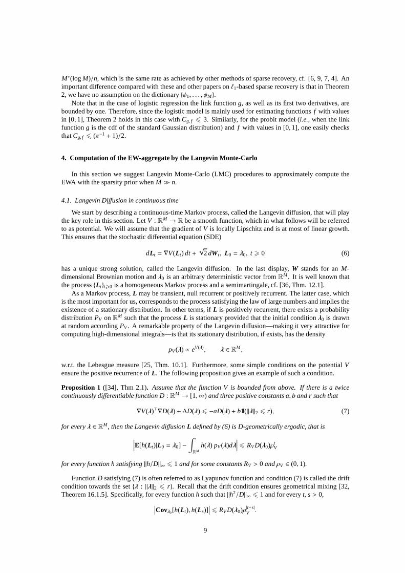
w.r.t. the Lebesgue measure [25, Thm. 10.1]. Furthermore, some simple conditions on the potentialVensure the positive recurrence ofL. The following proposition gives an example of such a condition.

Proposition 1 ([34], Thm 2.1). Assume that the function V is bounded from above. If there is atwicecontinuously differentiable function D: RM → [1,∞) and three positive constants a, b and r such that

∇V(λ)⊤∇D(λ) + ∆D(λ) 6 −aD(λ) + b1l(‖λ‖2 6 r), (7)

for everyλ ∈ RM, then the Langevin diffusionL defined by (6) is D-geometrically ergodic, that is

∣∣∣∣E[h(Lt)|L0 = λ0] −∫

RMh(λ) pV(λ)dλ

∣∣∣∣ 6 RVD(λ0)ρtV

for every function h satisfying‖h/D‖∞ 6 1 and for some constants RV > 0 andρV ∈ (0, 1).

FunctionD satisfying (7) is often referred to as Lyapunov function andcondition (7) is called the driftcondition towards the set{λ : ‖λ‖2 6 r}. Recall that the drift condition ensures geometrical mixing [32,Theorem 16.1.5]. Specifically, for every functionh such that‖h2/D‖∞ 6 1 and for everyt, s> 0,

∣∣∣Covλ0[h(Lt), h(Ls)]∣∣∣ 6 RVD(λ0)ρ|t−s|

V .

9

Combining this with the result of Proposition 1 it is not hardto check that if‖h2/D‖∞ 6 1, then

Eλ0

[( 1T

∫ T

0h(Lt)dt−

∫

RMh(λ)pV(λ)dλ

)2]6

CT, (8)

whereC is some positive constant depending only onV. Note also that, in view of Proposition 1, thesquared bias term in the bias-variance decomposition of theleft hand side of (8) is of orderO(T−2). Thus,the main error term comes from the stochastic part.

4.2. Langevin diffusion associated to EWA

In what follows, we focus on the particular caseg(x) = x. Given (Xi ,Yi), i = 1, . . . , n, with Xi ∈ RM

andYi ∈ R, we want to compute the expression

λ =

∫RM λexp

{ − β−1‖Y − Xλ‖22}π(dλ)

∫RM exp

{ − β−1‖Y − Xλ‖22}π(dλ)

, (9)

whereX = (X1, . . . , Xn)⊤. In what follows, we deal with the prior

π(dλ) ∝M∏

j=1

e−ω(αλ j )

(τ2 + λ2j )

2

assuming thatR = +∞. As proved in Sections 2 and 3, this choice of the prior leads to sharp oracleinequalities for a large class of noise distributions. An equivalent form for writing (9) is

λ =

∫

RMλpV(λ) dλ, wherepV(λ) ∝ eV(λ)

with

V(λ) = −‖Y − Xλ‖22

β−

M∑

j=1

{2 log(τ2

+ λ2j ) + ω(αλ j)

}. (10)

A simple algebra shows thatD(λ) = eα‖λ‖2 satisfies the drift condition (7). A nice property of thisLyapunov function is the inequality‖λ‖2∞ 6 α−1D(λ). It guarantees that (8) is satisfied for the functionsh(λ) = λi .

Let us define the Langevin diffusion Lt as solution of (6) with the potentialV given in (10) and theinitial conditionL0 = 0. In what follows we will consider only this particular diffusion process. We definethe average value

LT =1T

∫ T

0Lt dt, T > 0.

According to (8) this average value converges asT → ∞ to the vectorλ that we want to compute. Clearly,it is much easier to computeLT thanλ. Indeed,λ involves integrals inM dimensions, whereasLT is a one-dimensional integral over a finite interval. Of course, to compute such an integral one needs to discretizethe Langevin diffusion. This is done in the next subsection.

4.3. Discretization

Since the sample paths of a diffusion process are Holder continuous, it is easy to show thatthe Riemannsum approximation

LRT =

1T

N−1∑

i=0

LTi (Ti+1 − Ti),

with 0 = T0 < T1 < . . . < TN = T converges toLT in mean square when the sampling is sufficiently dense,that is when maxi |Ti+1 − Ti | is small. However, when simulating the diffusion sample path in practice, itis impossible to follow exactly the dynamics determined by (6). We need to discretize the SDE in order toapproximate the solution.

10

A natural discretization for the SDE (6) is proposed by the Euler scheme with a constant step of dis-cretizationh > 0, defined as

LEk+1 = LE

k + h∇V(LEk ) +

√2hξk, LE

0 = 0, (11)

for k = 0, 1, . . . , [T/h]−1,whereξ1, ξ2, . . . are i.i.d. standard Gaussian random vectors inRM and [x] stands

for the integer part ofx ∈ R. Obviously, the sequence{LEk ; k > 0} defines a discrete-time Markov process.

Furthermore, one can show that this Markov process can be extrapolated to a continuous-time diffusion-type process which converges in distribution to the Langevin diffusion ash→ 0. Here extrapolation meansthe construction of a process{Lt,h; t ∈ [0,T]} satisfying Lkh,h = LE

k for everyk = 0, . . . , [T/h]. Such aprocess{Lt,h; t ∈ [0,T]} can be defined as a solution of the SDE

dLt,h =

[T/h]−1∑

k=0

1l[k,k+1)(t/h)∇V(LEk ) dt+

√2dWt, t > 0.

This amounts to connecting the successive values of the Markov chain by independent Brownian bridges.The Girsanov formula implies that the Kullback-Leibler divergence between the distribution of the process{Lt; t ∈ [0,T]} and the distribution of{Lt,h

E; t ∈ [0,T]} tends to zero ash tends to zero. Therefore, it makessense to approximateLT by

LET,h =

hT

[T/h]−1∑

k=0

LEk .

Proposition 2. Consider the linear modelY = Xλ∗ + ξ, whereX is the n×M deterministic matrix andξ isa zero-mean noise with finite covariance matrix. Then forλ =

∫RM λ pV(λ) dλ with pV(λ) ∝ eV(λ) and V(λ)

defined in (10) we havelim

T→∞limh→0

E[∥∥∥LE

T,h − λ∥∥∥

2

]= 0.

Proof. We present here a high-level overview of the proof deferringthe details to the Appendix.

Step 1 We start by showing that

limh→0

E∥∥∥∥∥LE

T,h −1T

∫ T

0Lt,h dt

∥∥∥∥∥2

2= 0.

Step 2 We then split the expression1T∫ T

0Lt,h dt into two terms:

1T

∫ T

0Lt,h dt =

1T

∫ T

0Lt,h1l[0,A](‖Lt,h‖2) dt

︸ ︷︷ ︸T1

+1T

∫ T

0Lt,h1l]A,+∞](‖Lt,h‖2) dt

︸ ︷︷ ︸T2

. (12)

and show that the expected normE‖T2‖2 is bounded uniformly inh andT by some function ofA thatdecreases to 0 asA→ ∞. LaterA will be chosen as an increasing function ofT.

Step 3 We check that the Kullback-Leibler divergence between the distribution of (Lt,h; 0 6 t 6 T) andof (Lt; 0 6 t 6 T) tends to zero ash→ 0. This implies the convergence in total variation and, as aconsequence, we get

limh→0

E[( 1

T

∫ T

0G(Lt,h) dt−

∫

RMG(λ)pV(λ)dλ

)2]= E

[( 1T

∫ T

0G(Lt) dt−

∫

RMG(λ)pV(λ)dλ

)2](13)

for any bounded measurable functionG : RM → R. We use this result withG(λ) = λi1l[0,A](‖λ‖2),i = 1, . . . ,M.

Step 4 To conclude the proof we use the fact that∫‖λ‖2>A

λpV(λ) dλ tends to zero asA → ∞, and that bythe ergodic theorem (cf. Proposition 1) the right hand side of (13) tends to 0 asT → ∞.

11

This discretization algorithm is easily implementable and, for small values ofh, LET,h is very close to

the integralλ =∫λ pV(λ) dλ of interest. However, for some values ofh, which may eventually be small

but not enough, the Markov process{LEk ; k > 0} is transient. Therefore, ifh is not small enough the sum in

the definition ofLET,h explodes [35]. To circumvent this problem, one can either modify the Markov chain

LEk by incorporating a Metropolis-Hastings correction, or take a smallerh and restart the computations.

The Metropolis-Hastings approach guarantees the convergence to the desired distribution. However, itconsiderably slows down the algorithm because of a significant probability of rejection at each step ofdiscretization. The second approach, where we just take a smallerh, also slows down the algorithm but wekeep some control on its time of execution.

5. Implementation and experimental results

In this section we give more details on the implementation ofthe LMC for computing the EW-aggregatein the linear regression model.

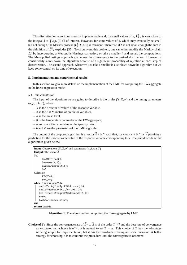
5.1. Implementation

The input of the algorithm we are going to describe is the triplet (Y,X, σ) and the tuning parameters(α, β, τ, h,T), where

- Y is then-vector of values of the response variable,- X is then× M matrix of predictor variables,- σ is the noise level,- β is the temperature parameter of the EW-aggregate,- α andτ are the parameters of the sparsity prior,- h andT are the parameters of the LMC algorithm.

The output of the proposed algorithm is a vectorλ ∈ RM such that, for everyx ∈ RM, x⊤λ provides aprediction for the unobservable value of the response variable corresponding tox. The pseudo-code of thealgorithm is given below.

Input: Observations (Y,X, σ) and parameters (α, β, τ, h,T)Output: The vectorλSet

[n,M]=size(X);

L=zeros(M,1);

lambda=zeros(M,1);

H=0;

CalculateXX=X’*X;

Xy=X’*y;

while H is less thanT donablaV=(2/β)*(Xy-XX*L)-α*ω′ (αL);nablaV=nablaV-4*L./(τ^2+L. 2);

L=L+h*nablaV+sqrt(2*h)*randn(M,1);

H=H+h;

lambda=lambda+h*L/T;endreturn lambda

Algorithm 1: The algorithm for computing the EW-aggregate by LMC.

Choice of T: Since the convergence rate ofLT to λ is of the orderT−1/2 and the best rate of convergencean estimator can achieve isn−1/2, it is natural to setT = n. This choice ofT has the advantageof being simple for implementation, but it has the drawback of being not scale invariant. A betterstrategy for choosingT is to continue the procedure until the convergence is observed.

12

Figure 2: A typical result of the EWA (left panel) and the Lasso (right panel) in the setup of Example 1 withn = 200,M = 500 andS = 20.

Choice of h: We choose the step of discretization in the form:h = β/(Mn) = β/Tr(X⊤X). More details onthe choice ofh andT will be given in a future work.

Choice of β, τ and α: In our simulations we use the parameter values

α = 0, β = 4σ2, τ = 4σ/(Tr(X⊤X))1/2 .

These values ofβ andτ are derived from the theory developed above. However, we take hereα = 0and notα > 0 as suggested in Section 3. We introduced thereα > 0 for theoretical convenience, inorder to guarantee the geometric mixing of the Langevin diffusion. Numerous simulations show thatmixing properties of the Langevin diffusion are preserved withα = 0 as well.

5.2. Numerical experiments

We present below two examples of application of the EWA with LMC for simulated data sets. Inboth examples we give also the results obtained by the Lasso procedure (rather as a benchmark, than forcomparing the two procedures). The main goal of this sectionis to illustrate the predictive ability of theEWA and to show that it can be easily computed for relatively large dimensions of the problem. In allexamples the Lasso estimators are computed with the theoretically justified value of the regularaizationparameterσ

√8 logM/n (cf. [4]).

5.2.1. Example 1This is a standard numerical example where the Lasso and Dantzig selector are known to behave well

(cf. [9]). Consider the modelY = Xλ∗ +σξ, whereX is aM × n matrix with independent entries, such thateach entry is a Rademacher random variable. Such matrices are particularly well suited for applicationsin compressed sensing. The noiseξ ∈ Rn is a vector of independent standard Gaussian random variables.The vectorλ∗ is chosen to beS-sparse, whereS is much smaller thanM. W. l. o. g. we consider vectorsλ∗

such that only firstS coordinates are different from 0; more precisely,λ∗j = 1l( j 6 S). Following [9], we

chooseσ2= S/9. We run our procedure for several values ofS andM. The results of 500 replications are

summarized in Table 1. We see that EWA outperforms Lasso in all the considered cases.A typical scatterplot of estimated coefficients forM = 500,n = 200 andS = 20 is presented in Fig. 2.

The left panel shows the estimated coefficients obtained by EWA, while the right panel shows the estimatedcoefficients obtained by Lasso. One can clearly see that the estimated values provided by EWA are muchmore accurate than those provided by Lasso.

An interesting observation is that the EWA selects the set ofnonzero coordinates ofλ∗ even better thanthe Lasso does. In fact, the approximate sparsity of the EWA is not very surprising, since in the noise-freelinear models with orthogonal matrixX, the symmetry of the prior implies that the EWA recovers the zerocoordinates without error.

13

M = 100 M = 200 M = 500EWA Lasso EWA Lasso EWA Lasso

n = 100S = 5 0.063 0.344 0.064 0.385 0.087 0.453(0.039) (0.132) (0.043) (0.151) (0.054) (0.161)

n = 100S = 10 0.73725 1.680 1.153 1.918 1.891 2.413(0.699) (0.621) (1.091) (0.677) (1.522) (0.843)

n = 100S = 15 5.021 4.330 6.495 5.366 8.917 7.1828(1.593) (1.262) (1.794) (1.643) (2.186) (2.069)

n = 200S = 5 0.021 0.151 0.022 0.171 0.019 0.202(0.011) (0.048) (0.013) (0.055) (0.012) (0.057)

n = 200S = 10 0.106 0.658 0.108 0.753 0.117 0.887(0.047) (0.169) (0.048) (0.198) (0.051) (0.239)

n = 200S = 20 1.119 3.124 1.6015 3.734 2.728 4.502(0.696) (0.806) (1.098) (0.907) (1.791) (1.063)

Table 1: Average loss‖λ − λ∗‖2 of the estimators obtained by the EW-aggregate and the Lassoin Example 1. The standard deviationis given in parentheses.

We note that the numerical results on the Lasso in Table 5.2.1are substantially different from thosereported in the short version of this paper published in the Proceeding of COLT 2009 [17]. This is becausein [17] we used the R packageslars andglmnet, whereas here we use the MATLAB packagel1_ls. Itturns out that in the present example the latter provides more accurate approximation of the Lasso than theaforementioned R packages.

The running times of our algorithm are reasonable. For instance, in the casen = m = 100 andS = 10the execution of our algorithm is only three times longer than thel1-ls implementation of the Lasso. Onthe other hand, the prediction error of our algorithm is morethan twice smaller than that of the Lasso.

5.2.2. Example 2

Consider model (1) whereZi are independent random variables uniformly distributed inthe unit square[0, 1]2 andξi are iidN(0, σ2) random variables. For an integerk > 0, we consider the indicator functionsof rectangles with sides parallel to the axes and having as left-bottom vertex the origin and as right-topvertex a point of the form (i/k, j/k), (i, j) ∈ N2. Formally, we defineφ j by

φ(i−1)k+ j(x) = 1l[0,i]×[0, j](kx), ∀ x ∈ [0, 1]2.

The underlying imagef we are trying to recover is taken as a superposition of a smallnumber of rectanglesof this form, that isf (x) =

∑k2

ℓ=1 λ∗ℓφℓ(x), for all x ∈ [0, 1]2 with someλ∗ having a smallℓ0-norm. We set

k = 15,‖λ∗‖0 = 3, λ∗10 = λ∗100 = λ

∗200 = 1. Thus, the cardinality of the dictionary isM = k2

= 225.In this example the functionsφ j are strongly correlated and therefore the assumptions likerestricted

isometry or low coherence are not fulfilled. Nevertheless, the Lasso succeeds in providing an accurateprediction (cf. Table 2). Furthermore, the Lasso with the theoretically justified choice of the regularizationparameterσ

√8 logM/n is not much worse than the ideal Lasso-Gauss (LG) estimator.We call the LG

estimator the ordinary least squares estimator in the reduced model where only the predictor variablesselected at a preliminary Lasso step are kept. Of course, theperformance of the LG procedure depends onthe initial choice of the tuning parameter for the Lasso step. In our simulations, we use its ideal (oracle)value minimizing the prediction error and, therefore, we call the resulting procedure the ideal LG estimator.

As expected, the EWA has a smaller predictive risk than the Lasso estimator. However, a surprisingoutcome of this experiment is the supremacy of the EWA over the ideal LG in the case of large noisevariance. Of course, the LG procedure is faster. However, even from this point of view the EWA is ratherattractive, since it takes less than two seconds to compute it in the present example.

14

EWA Lasso Ideal LG

σ = 1, n = 100 0.160 0.273 0.128(0.035) (0.195) (0.053)

σ = 2, n = 100 0.210 0.759 0.330(0.072) (0.562) (0.145)

σ = 4, n = 100 0.420 2.323 0.938(0.222) (1.257) (0.631)

σ = 1, n = 200 0.130 0.187 0.069(0.030) (0.124) (0.031)

σ = 2, n = 200 0.187 0.661 0.203(0.048) (0.503) (0.086)

σ = 4, n = 200 0.278 2.230 0.571(0.132) (1.137) (0.324)

Table 2: Average loss∫[0,1]2

(∑j (λ j − λ∗j )φ j (x)

)2 dx of the the EWA, the Lasso and the ideal LG procedures in Example 2. Thestandard deviation is given in parentheses.

Figure 3: This figure shows a typical outcome in the setup of example 2 whenn = 200 andk = 15. Left: the original image.Center:the observed noisy sample withσ = 0.5. Pixels for which no observation is available are in black.Right: the image estimated by theEWA.

6. Conclusion and outlook

This paper contains two contributions: New oracle inequalities for EWA, and the LMC method forapproximate computation of the EWA. The first oracle inequality presented in this work is in the line of thePAC-Bayesian bounds initiated by McAllester [30]. It is valid for any prior distribution and gives a boundon the risk of the EWA with an arbitrary family of functions. Next, we derive another inequality, whichis adapted to the sparsity scenario and called the sparsity oracle inequality (SOI). In order to obtain it, wepropose a prior distribution favoring sparse representations. The resulting EWA is shown to behave almostas well as the best possible linear combination within a residual term proportional toM∗(log M)/n, whereM is the true dimension,M∗ is the number of atoms entering in the best linear combination andn is thesample size. A remarkable fact is that this inequality is obtained under no condition on the relationshipbetween different atoms.

Sparsity oracle inequalities similar to that of Theorem 2 are valid for the penalized empirical riskminimizers (ERM) with aℓ0-penalty (proportional to the number of atoms involved in the representation).It is also well known that the problem of computing theℓ0-penalized ERM is NP-hard. In contrast withthis, we have shown that the numerical evaluation of the suggested EWA is a computationally tractableproblem. We demonstrated that it can be efficiently solved by the LMC algorithm. Numerous simulationswe did (some of which are included in this work) confirm our theoretical findings and, furthermore, suggestthat the EWA is able to efficiently select the sparsity pattern. Theoretical justification of this fact, as wellas more thorough investigation of the choice of parameters involved in the LMC algorithm, are interestingtopics for future research.

15

Appendix: proofs of technical results

6.1. Proof of Proposition 2

For brevity, in this proof we denote by‖ · ‖ the Euclidean norm inRM and we setα = 1 in (10).The case of generalα > 0 is treated analogously. Recall that for some smallh > 0 we have defined theM-dimensional Markov chain (LE

k ; k = 0, 1, 2, . . .) by (cf. (10) and (11)):

LEk+1 = LE

k + 2hβ−1X⊤(Y − XLE

k ) − hg(LEk ) +

√2hξk+1, LE

0 = 0,

where (ξk; k = 1, 2, . . .) is a sequence of iid standard Gaussian vectors inRM, and

g : RM → RM s.t. g(λ) =

( 4λ1

τ2 + λ21

+ ω′(λ1), . . . ,4λM

τ2 + λ2M

+ ω′(λM))⊤.

In what follows, we will use the fact that the functiong is bounded and satisfiesλ⊤g(λ) > 0 for all λ ∈ RM.Let us prove some auxiliary results. Setv = 2β−1

X⊤Y, A = 2β−1

X⊤X and assume thath 6 1/‖A‖.

Without loss of generality we also assume thatT/h is an integer. In what follows, we denote byC > 0 aconstant whose value is not essential, does not depend neither onT nor onh, and may vary from line toline. Since the functiong is bounded andξk+1 has zero mean, we have

E[LEk+1] = (I − hA)E[LE

k ] + hE[v − g(LEk )], ∀k > 0.

Therefore,‖E[LE

k+1]‖ 6 ‖(I − hA)E[LEk ]‖ +Ch6 ‖E[LE

k ]‖ +Ch, ∀k > 0.

By induction, we get‖E[LE

k ]‖ 6 Ckh6 CT, ∀k ∈ [0, [T/h]] . (14)

Furthermore, sinceξk+1 is independent ofLEk andY, we have

E[‖LEk+1‖2] = E[‖LE

k + hv − hALEk − hg(LE

k )‖2] + 2hM

6 E[‖LEk ‖2 + 2h(LE

k )⊤(v − ALEk ) − 2h(LE

k )⊤g(LEk ) + h2‖v − ALE

k − g(LEk )‖2] + 2hM

6 E[‖LEk ‖2 + 2h(LE

k )⊤(v − ALEk ) + 2h2‖ALE

k ‖2 + 2h2‖v − g(LEk )‖2] + 2hM

6 E[‖LEk ‖2 + 2h(LE

k )⊤v − 2h(LEk )⊤(A − hA2)LE

k + 2h2‖v − g(LEk )‖2] + 2hM

6 E[‖LEk ‖2] + 2hE[(LE

k )⊤]v +Ch

6 E[‖LEk ‖2] +ChT, ∀k ∈ [0, [T/h]] .

Once again, using induction, we get

E[‖LEk ‖2] 6 CkhT6 CT2, ∀k ∈ [0, [T/h]] . (15)

This implies, in particular, that (h/T)E[‖LE[T/h]‖2] → 0 ash→ 0 for any fixedT.

Proof of Step 1. Denote byψ the function

ψ(λ) = v − Aλ − g(λ), ∀λ ∈ RM ,

and define the continuous-time random process (Lt,h; 0 6 t 6 [T/h]h) by

dLt,h =

[T/h]−1∑

k=0

ψ(LEk )1l[kh,(k+1)h)(t) dt+

√2dWt, L0,h = 0, (16)

whereWt is a M-dimensional Brownian motion satisfyingWkh = ξk, for all k. The rigorous constructionof W can be done as follows. Let (Bt; 0 6 t 6 T) be aM-dimensional Brownian motion defined on the

16

same probability space as the sequence (ξk; 0 6 k 6 [T/h]) and independent of (ξk; 0 6 k 6 [T/h]). Onecan check that the process defined by

Wt = ξk + Bt − Bkh −( th− k

)(B(k+1)h − Bkh− ξk+1

), t ∈ [kh, (k+ 1)h[

is a Brownian motion and satisfiesWkh = ξk.By the Cauchy-Schwarz inequality,

E[∥∥∥∥∥

hT

[T/h]−1∑

k=0

LEk −

1T

∫ T

0Lt,h dt

∥∥∥∥∥2]= E

[∥∥∥∥∥1T

∫ T

0

( [T/h]−1∑

k=0

Lkh,h1l[kh,(k+1)h)(t) − Lt,h)dt

∥∥∥∥∥2]

61T

[T/h]−1∑

k=0

∫ (k+1)h

khE[‖Lt,h − Lkh,h‖2

]dt

62T

[T/h]−1∑

k=0

(k+1)h∫

kh

E[h2‖ψ(LE

k )‖2 + 2‖Wt −Wkh‖2]dt

62h3

T

[T/h]−1∑

k=0

E[‖ψ(LE

k )‖2] + 4Mh.

Using the inequality‖ψ(λ)‖ 6 C(1+ ‖λ‖) and (15), we get

E[∥∥∥∥∥

hT

[T/h]−1∑

k=0

LEk −

1T

∫ T

0Lt,h dt

∥∥∥∥∥2]

6 Ch2+

Ch3

T

[T/h]−1∑

k=0

E[‖LE

k ‖2]+ 4Mh

6 Ch(1+ hT2).

This completes the proof of the Step 1.

Proof of Step 2. Using (15) we obtain

E[‖T2‖] 61T

∫ T

0E[‖Lt,h‖1l[A,+∞](‖Lt,h‖)] 6

1T A

∫ T

0E[‖Lt,h‖2] dt

6C

T A

[T/h]−1∑

k=0

∫ (k+1)h

kh

(E[‖LE

k ‖2] + h2E[‖ψ(LEk ) + ALE

k ‖2] + E[‖Wt −Wkh‖2])dt

6C

T A

[T/h−1]∑

k=0

h(E[‖LE

k ‖2] +Ch2+ Mh

)6

CT2

A. (17)

Thus, choosing, for example,A = T3 we guarantee that limT→∞ limh→0 E[‖T2‖] = 0.

Proof of Step 3. First, note that (16) can be written in the form

dLt,h = ψ(Lh, t) dt+√

2dWt, L0,h = 0,

whereψ(Lh, t) is a non-anticipative process that equalsψ(Lkh,h) when t ∈ [kh, (k + 1)h). Recall that theLangevin diffusion is defined by the stochastic differential equation

dLt = ψ(Lt) dt+√

2dWt, L0 = 0.

Therefore, the probability distributionsPL,T and PLh,T induced by, respectively, (Lt; 0 6 t 6 T) and(Lt,h; 0 6 t 6 T) are mutually absolutely continuous and the correspondingRadon-Nykodim derivativesare given by Girsanov formula:

dPLh,T

dPL,T(L) = exp

{ 1√

2

∫ T

0(ψ(L, t) − ψ(Lt))⊤

(dLt − ψ(Lt) dt

) − 14

∫ T

0‖ψ(L, t) − ψ(Lt)‖2 dt

}.

17

This implies that the Kullback-Leibler divergence betweenPLh,T andPL,T is given by

K(PL,T ||PLh,T

)= −E

[log

(dPLh,T

dPL,T(L)

)]=

14

∫ T

0E[‖ψ(L, t) − ψ(Lt)‖2

]dt.

Using the expressions ofψ andψ, as well as the fact that the functionψ is Lipschitz continuous, we canbound the divergence above as follows:

K(PL,T ||PLh,T

)=

14

[T/h]−1∑

k=0

∫ (k+1)h

khE[‖ψ(Lkh) − ψ(Lt)‖2

]dt

6 C[T/h]−1∑

k=0

∫ (k+1)h

khE[‖Lkh− Lt‖2

]dt

= C[T/h]−1∑

k=0

∫ (k+1)h

khE[∥∥∥∥

∫ t

khψ(Ls) ds+

√2(Wt −Wkh)

∥∥∥∥2]

dt.

From the Cauchy-Schwarz inequality and the fact that‖ψ(λ)‖ 6 C(1+ ‖λ‖) we obtain

K(PL,T ||PLh,T

)6 C

[T/h]−1∑

k=0

∫ (k+1)h

khh∫ t

khE[‖ψ(Ls)‖2

]ds dt+ChT

6 Ch2[T/h]−1∑

k=0

∫ (k+1)h

khE[‖ψ(Ls)‖2

]ds+ChT

6 Ch2∫ T

0E[‖ψ(Ls)‖2

]ds+ChT

6 Ch2∫ T

0E[‖Ls‖2

]ds+ChT.

Since by Proposition 1 the expectation of‖Ls‖2 is bounded uniformly ins, we getK(PL,T ||PLh,T

) → 0 ash → 0. In view of Pinsker’s inequality, cf, e.g., [38], this implies that the distributionPLh,T converges toPL,T in total variation ash→ 0. Thus, (13) follows.

Proof of Step 4. To prove that the right hand side of (13) tends to zero asT → +∞, we use the fact that theprocessLt has the geometrical mixing property withD(λ) = eα‖λ‖2. Bias-variance decomposition yields:

E[( 1

T

∫ T

0G(Lt) dt−

∫G(λ)pV(λ)dλ

)2]=

1T2

Var[ ∫ T

0G(Lt) dt

]+

( 1T

∫ T

0E0[G(Lt)] dt−

∫G(λ)pV(λ)dλ

)2

.

The second term on the right hand side of the last display tends to zero asT → ∞ in view of Proposition 1,while the first term can be evaluated as follows:

1T2

Var[ ∫ T

0G(Lt) dt

]=

1T2

∫ T

0

∫ T

0Cov0

[G(Lt),G(Ls)

]dt ds

6CT2

∫ T

0

∫ T

0ρ−|t−s|V dt ds6 CT−1.

This completes the proof of Proposition 2.

6.2. Proof of Lemma 3

We first prove a simple auxiliary result, cf. Lemma 4 below. Then, the two claims of Lemma 3 areproved in Lemmas 5 and 6, respectively.

18

Lemma 4. For every M∈ N and every s> M, the following inequality holds:

1(π/2)M

∫{u:‖u‖1>s

}M∏

j=1

duj

(1+ u2j )

26

M(s− M)2

.

Proof. Let U1, . . . ,UM be iid random variables drawn from the scaled Studentt(3) distribution having asdensity the functionu 7→ 2/

[π(1+u2)2]. One easily checks thatE[U2

1] = 1. Furthermore, with this notation,we have

1(π/2)M

∫{u:‖u‖1>s

}M∏

j=1

duj

(1+ u2j )

2= P

( M∑

j=1

|U j | > s).

In view of Chebyshev’s inequality the last probability can be bounded as follows:

P( M∑

j=1

|U j | > s)6

ME[U21]

(s− ME[|U1|])26

M(s− M)2

and the desired inequality follows.

Lemma 5. Let the assumptions of Theorem 2 be satisfied and let p0 be the probability measure defined by(5). If M > 2 then ∫

Λ

(λ1 − λ∗1)2p0(dλ) 6 4τ2e4Mατ.

Proof. Using the change of variablesu = (λ − λ∗)/τ we write

∫

Λ

(λ1 − λ∗1)2p0(dλ) = CMτ2∫

B1(2M)u2

1

( M∏

j=1

(1+ u2j )−2e−ω(ατuj )

)du

with

CM =( ∫

B1(2M)

( M∏

j=1

(1+ u2j )−2e−ω(ταuj )

)du

)−1(18)

whereu j are the components ofu. Bounding the functionse−ω(ταuj ) by one, extending the integration fromB1(2M) to R

M and using the inequality∫R

u21(1+ u2

1)−2du1 6 π, we get

∫

Λ

(λ1 − λ∗1)2p0(dλ) 6 CMτ2π

( ∫

R

(1+ t2)−2 dt)M−1

= 2CMτ2(π/2)M,

where we used that the primitive of the function (1+ x2)−2 is 12 arctan(x) + x

2(1+x2) . To boundCM we firstuse the inequality ¯ω(x) 6 2|x| which yields:

CM 6( ∫

B1(2M)e−2ατ‖u‖1

M∏

j=1

duj

(1+ u2j )

2

)−16 e4ατM

( ∫

B1(2M)

M∏

j=1

duj

(1+ u2j )

2

)−1. (19)

In view of (19) and Lemma 3 we have

CM 6 e4ατM(2/π)M(1− 1/M

)−16 2e4ατM(2/π)M (20)

for M > 2. Combining these estimates we get∫

Λ

(λ1 − λ∗1)2p0(dλ) 6 4τ2e4ατM

and the desired inequality follows.

19

Lemma 6. Let the assumptions of Theorem 2 be satisfied and let p0 be the probability measure defined by(5). Then

K(p0, π) 6 2(α‖λ∗‖1 +

M∑

j=1

2 log(1+ |λ∗j |/τ))+ (1+ 4Mατ).

Proof. The definition ofπ, p0 and of the Kullback-Leibler divergence imply that

K(p0, π) =∫

B1(2Mτ)log

{CMCα,τ,R

∏Mj=1

(τ2+λ2

j )2eω(αλj )

(τ2+(λj−λ∗j )2)2eω(α(λj−λ∗j ))

}p0(dλ)

= log(CMCα,τ,R) + 2∑M

j=1

∫B1(2Mτ)

log

{τ2+λ2

j

τ2+(λj−λ∗j )2

}p0(dλ)

+∑M

j=1

∫B1(2Mτ)

(ω(αλj) − ω(α(λj − λ∗j ))

)p0(dλ). (21)

We now successively evaluate the three terms on the RHS of (21). First, in view of (4), we have

Cα,τ,R =

∫

B1(R)

M∏

j=1

e−ω(αujτ)

(1+ u2j )

2duj 6

( ∫

R

(1+ u2j )−2 duj

)M= (π/2)M.

This and (20) imply log(CMCα,τ,R) 6 1+ 4Mατ.To evaluate the second term on the RHS of (21) we use that

τ2+ λ2

j

τ2 + (λj − λ∗j )2= 1+

2τ(λj − λ∗j )

τ2 + (λj − λ∗j )2(λ∗j /τ) +

λ∗j2

τ2 + (λj − λ∗j )2

6 1+ |λ∗j /τ| + (λ∗j /τ)26 (1+ |λ∗j /τ|)2.

This entails that the second term on the RHS of (21) is boundedfrom above by∑M

j=1 2 log(1+ |λ∗j |/τ).Finally, since the derivative of ¯ω(·) is bounded in absolute value by 2, we have ¯ω(αλj) − ω(α(λj − λ∗j )) 62α|λ∗j | which implies:

M∑

j=1

∫

B1(2Mτ)

(ω(αλj) − ω

(α(λj − λ∗j )

))p0(dλ) 6 2α‖λ∗‖1.

Combining these inequalities we get the lemma.

6.3. Proofs of remarks 1-6

We only prove Remarks 2 and 6, since the proofs of the remaining remarks are straghtforward.

6.3.1. Proof of Remark 2Let ξ be a random variable satisfyingP(ξ = ±σ) = 1/2 and letU be another random variable, inde-

pendent ofξ and drawn from the uniform distribution on [−1, 1]. Recall thatζ = (1+ γ)σ sgn[σ−1ξ − (1+γ)U] − ξ.

We start by proving thatξ + ζ has the same distribution as (1+ γ)ξ. Clearly, |ξ + ζ | equals (1+ γ)σalmost surely. Furthermore,

P(ξ + ζ = (1+ γ)σ

)= P

(σ−1ξ > (1+ γ)U

)

=12

(P(1 > (1+ γ)U

)+ P

( − 1 > (1+ γ)U))

=14

(( 11+ γ

+ 1)+

(− 1

1+ γ+ 1

))=

12.

This entails thatP(ξ+ ζ = −(1+ γ)σ

)= 1/2 and, therefore, the distributions ofξ + ζ and (1+ γ)ξ coincide.

20

We compute now the conditional expectationE[ζ |ξ]. SinceU andξ are independent, we have

E[ζ | ξ = σ] = (1+ γ)σE(sgn[1− (1+ γ)U]

) − σ = 0.

Similarly, E[ζ | ξ = −σ] = 0.To complete the proof of Remark 2, it remains to show that partiii) of Assumption N is fulfilled. Indeed,

logE[etζ | ξ = σ]t2γσ2

=1

t2γσ2log

(etγσ 2+ γ

2(1+ γ)+ e−t(2+γ)σ γ

2(1+ γ)

)

=1

t2γσ2

[tγσ + log

(1+

{e−2t(1+γ)σ − 1

}γ

2(1+ γ)

)].

Applying the inequality of [16, Lemma 3] withα0 = 2(1+ γ)/γ andx = tγσ, we get

logE[etζ | ξ = σ]t2γσ2

61

t2γσ2(tγσ)2 (1+ γ)

γ= 1+ γ

and the desired result follows.

6.3.2. Proof of Remark 6We start by computing the conditional moment generating function (Laplace transform) ofζ givenξ:

E[etζ

∣∣∣ ξ = a]= e−taE

[et(ζ+ξ)

∣∣∣ ξ = a]

= e−ta

(et(1+γ)|a|P

(sgn(a) > (1+ γ)U

)+ e−t(1+γ)|a|P

(sgn(a) < (1+ γ)U

))

= e−ta

(et(1+γ)a 2+ γ

2+ 2γ+ e−t(1+γ)a γ

2+ 2γ

). (22)

Using (22) we obtain

E[et(ζ+ξ)]

= E[E[et(ζ+ξ)

∣∣∣ ξ]]=

2+ γ2+ 2γ

E[e−t(1+γ)ξ]

+γ

2+ 2γE[et(1+γ)ξ]

= E[et(1+γ)ξ],

since the symmetry ofξ implies thatE[e−t(1+γ)ξ]

= E[et(1+γ)ξ] for every t. Thus, ζ + ξ has the same

distribution as (1+ γ)ξ.On the other hand, taking the derivatives of both sides of (22) and using the fact thatE[ζ | ξ = a] equals

to the derivative of the moment generating functionE[etζ | ξ = a] at t = 0, we obtain thatE[ζ | ξ = a] = 0for everya ∈ [−B, B]. To complete the proof of Remark 6 we apply [16, Lemma 3] to the right hand sideof (22). This yields

log(E[etζ

∣∣∣ ξ = a])

6 (tγa)21+ γγ

6 (tB)2γ(1+ γ).

Therefore, part iii) of Assumption N is satisfied withv(a) 6 B2. This completes the proof of Remark 6.

References

[1] Abramovich, F., Grinshtein, V., Pensky, M., 2007. On optimality of Bayesian testimation in the nor-mal means problem. Ann. Statist. 35, 2261–2286.

[2] Alquier, P., 2008. Pac-Bayesian bounds for randomized empirical risk minimizers. Math. MethodsStatist. 17 (4), 1–26.

[3] Audibert, J.-Y., 2009. Fast learning rates in statistical inference through aggregation. Ann. Statist.37 (4), 1591–1646.

21

[4] Bickel, P. J., Ritov, Y., Tsybakov, A. B., 2009. Simultaneous analysis of lasso and Dantzig selector.Ann. Statist. 37 (4), 1705–1732.

[5] Bunea, F., Tsybakov, A., Wegkamp, M., 2007. Sparsity oracle inequalities for the Lasso. ElectronicJ. of Statist. 1, 169–194.

[6] Bunea, F., Tsybakov, A. B., Wegkamp, M., 2006. Aggregation and sparsity vial1 penalized leastsquares. In: Learning theory. Vol. 4005 of Lecture Notes in Comput. Sci. Springer, Berlin, pp. 379–391.

[7] Bunea, F., Tsybakov, A. B., Wegkamp, M., 2007. Aggregation for Gaussian regression. Ann. Statist.35 (4), 1674–1697.

[8] Candes, E., Tao, T., 2006. Near-optimal signal recovery from random projections: universal encodingstrategies? IEEE Trans. Inform. Theory 52 (12), 5406–5425.

[9] Candes, E., Tao, T., 2007. The Dantzig selector: statistical estimation whenp is much larger thann.Ann. Statist. 35 (6), 2313–2351.

[10] Catoni, O., 2004. Statistical learning theory and stochastic optimization. Lecture Notes in Mathemat-ics. Springer-Verlag, Berlin.

[11] Catoni, O., 2007. Pac-Bayesian Supervised Classification: The Thermodynamics of Statistical Learn-ing. Vol. 56. IMS Lecture Notes Monograph Series.

[12] Cesa-Bianchi, N., Conconi, A., Gentile, C., 2004. On the generalization ability of on-line learningalgorithms. IEEE Trans. Inform. Theory 50 (9), 2050–2057.

[13] Cesa-Bianchi, N., Freund, Y., Haussler, D., Helmbold,D. P., Schapire, R. E., Warmuth, M. K., 1997.How to use expert advice. J. ACM 44 (3), 427–485.

[14] Cesa-Bianchi, N., Lugosi, G., 2006. Prediction, learning, and games. Cambridge University Press,Cambridge.

[15] Dalalyan, A. S., Tsybakov, A. B., 2007. Aggregation by exponential weighting and sharp oracleinequalities. In: Learning theory. Vol. 4539 of Lecture Notes in Comput. Sci. Springer, Berlin, pp.97–111.

[16] Dalalyan, A. S., Tsybakov, A. B., 2008. Aggregation by exponential weighting, sharp PAC-Bayesianbounds and sparsity. Mach. Learn. 72 (1-2), 39–61.

[17] Dalalyan, A. S., Tsybakov, A. B., 2009. Sparse regression learning by aggregation and LangevinMonte-Carlo. In: COLT-2009.

[18] Donoho, D., Elad, M., Temlyakov, V., 2006. Stable recovery of sparse overcomplete representationsin the presence of noise. IEEE Trans. Inform. Theory 52 (1), 6–18.

[19] Efron, B., Hastie, T., Johnstone, I., Tibshirani, R., 2004. Least angle regression. Ann. Statist. 32 (2),407–499.

[20] Gaıffas, S., Lecue, G., 2007. Optimal rates and adaptation in thesingle-index model using aggrega-tion. Electron. J. Stat. 1, 538–573.

[21] Giraud, C., Huet, S., Verzelen, N., 2009. Graph selection with GGMselect. preprint, available onarXiv:0907.0619v1.

[22] Haussler, D., Kivinen, J., Warmuth, M., 1998. Sequential prediction of individual sequences undergeneral loss functions. IEEE Trans. Inform. Theory 44 (5), 1906–1925.

[23] Johnstone, I., Silverman, B., 2005. Empirical Bayes selection of wavelet thresholds. Ann. Statist 33,1700–1752.

22

[24] Juditsky, A., Rigollet, P., Tsybakov, A., 2008. Learning by mirror averaging. Ann. Statist. 36, 2183–2206.

[25] Kent, J., 1978. Time-reversible diffusions. Adv. in Appl. Probab. 10 (4), 819–835.

[26] Kivinen, J., Warmuth, M. K., 1999. Averaging expert predictions. In: Computational learning theory(Nordkirchen, 1999). Vol. 1572 of Lecture Notes in Comput. Sci. Springer, Berlin, pp. 153–167.

[27] Koltchinskii, V., 2009. Sparse recovery in convex hulls via entropy penalization. Ann. Statist. 37 (3),1332–1359.

[28] Leung, G., Barron, A., 2006. Information theory and mixing least-squares regressions. IEEE Trans.Inform. Theory 52 (8), 3396–3410.

[29] Littlestone, N., Warmuth, M. K., 1994. The weighted majority algorithm. Inform. and Comput.108 (2), 212–261.

[30] McAllester, D., 2003. Pac-Bayesian stochastic model selection. Machine Learning 51 (1), 5–21.

[31] Meinshausen, N., Buhlmann, P., 2006. High-dimensional graphs and variable selection with theLasso. Ann. Statist. 34 (3), 1436–1462.

[32] Meyn, S. P., Tweedie, R. L., 1993. Markov chains and stochastic stability. Communications andControl Engineering Series. Springer-Verlag London Ltd.,London.

[33] Rivoirard, V., 2006. Non linear estimation over weak Besov spaces and minimax Bayes method.Bernoulli 12 (4), 609–632.

[34] Roberts, G., Stramer, O., 2002. Langevin diffusions and Metropolis-Hastings algorithms. Methodol.Comput. Appl. Probab. 4 (4), 337–357.

[35] Roberts, G. O., Stramer, O., 2002. Langevin diffusions and Metropolis-Hastings algorithms.Methodol. Comput. Appl. Probab. 4 (4), 337–357 (2003), international Workshop in Applied Proba-bility (Caracas, 2002).

[36] Rogers, L., Williams, D., 1987. Diffusions, Markov processes, and martingales. Vol. 2. Probabilityand Mathematical Statistics. John Wiley & Sons Inc., New York.

[37] Seeger, M. W., 2008. Bayesian inference and optimal design for the sparse linear model. J. Mach.Learn. Res. 9, 759–813.

[38] Tsybakov, A. B., 2008. Introduction to Nonparametric Estimation. Springer Publishing Company,Incorporated.

[39] van de Geer, S., 2008. High-dimensional generalized linear models and the Lasso. Ann. Statist. 36 (2),614–645.

[40] Vovk, V., 1990. Aggregating strategies. In: COLT: Proceedings of the Workshop on ComputationalLearning Theory, Morgan Kaufmann Publishers. pp. 371–386.

[41] Vovk, V. G., 1989. Prediction of stochastic sequences.Problemy Peredachi Informatsii 25 (4), 35–49.

[42] Wipf, D. P., Rao, B. D., 2007. An empirical Bayesian strategy for solving the simultaneous sparseapproximation problem. IEEE Trans. Signal Process. 55 (7, part 2), 3704–3716.

[43] Yang, Y., 2004. Aggregating regression procedures to improve performance. Bernoulli 10 (1), 25–47.

[44] Yu, B., 2007. Embracing statistical challenges in the information technology age. Technometrics49 (3), 237–248.

[45] Zhang, C., Huang, J., 2008. The sparsity and biais of theLasso selection in high-dimensional linearregression. Ann. Statist. 36, 1567–1594.

23

[46] Zhao, P., Yu, B., 2006. On model selection consistency of Lasso. J. Mach. Learn. Res. 7, 2541–2563.

[47] Zou, H., Hastie, T., 2005. Regularization and variableselection via the elastic net. J. R. Stat. Soc. Ser.B 67 (2), 301–320.

24