SOPS

Stochastic Optimization in Policy Space

User’s Manual

Version 1.0 October 2010

2

Content

FOREWORD 3

1. STOCHASTIC OPTIMIZATION IN POLICY SPACE 4

2. MODELLING WITH POWERSIM STUDIO 8 2.1. Modelling 8 2.2. Simulating 9 2.3. Beginner’s hints for Powersim Studio 9

3. SOPS POLICY FUNCTIONS 11 3.1. Grid policy functions 11 3.1. Custom policies 14

4. TRANSFERRING FROM STUDIO TO SOPS 16

5. OPTIMIZING WITH SOPS 18

6. ANALYZING RESULTS 30

APPENDIX 1: INSTALLING PROGRAMS 35

APPENDIX 2: EXAMPLE MODEL EQUATIONS 36

3

FOREWORD

It is now well established that people have difficulties making good decisions in nonlinear dynamic systems and in the presence of uncertainty. When these challenges are combined, decision problems get even worse. One way to deal with such problems is to use stochastic dynamic programming (SDP). Unfortunately the mathematics of SDP is complicated and the available software packages are not intended for non-specialists. Furthermore, SDP is traditionally limited to quite small and well defined problems, often different from the more complex problems people have to deal with in practice.

Stochastic optimisation in policy space (SOPS) is an attractive alternative,

particularly for people with a background in simulation. Rather than transforming the simulation model to a transition matrix and solving the problem backwards in time as in SDP, SOPS tries out different policy alternatives on a large number of simulated scenarios. This is done by Monte Carlo simulations. The average outcome over all scenarios represents the expected outcome or expected utility of a policy. A search routine finds the policy that maximizes the expected utility. With this method one finds the same optimal solutions as one would find with SDP for problems of limited size. In addition, one can find near-to-optimal policies for more complex problems.

Optimizing with SOPS consists of three stages. First the underlying dynamic

model is formulated and tested in the graphically oriented simulation program Powersim Studio. The graphics help the intuitive understanding of the model. The simulation capabilities enable extensive testing of the model. Once testing is finished, one mouse click brings the user directly to the optimization program SOPS. In this second stage the user specifies randomness, starting values for policies, and desired accuracy before the optimization is executed. For small simulation models, it may take no more than a couple of minutes from finishing the simulation model to seeing the first optimization results. The resulting policies are reported in tables. In a third stage, these tables are easily copied to Excel, statistical packages, and Studio for storage, analysis, and production of graphs.

This user’s manual is organized according to the three stages. After a quick

introduction to optimization, it starts with model formulations in Powersim Studio, goes through optimization in SOPS, and ends with analysis of results in Excel and Studio. A first appendix explains how to obtain and install needed software. A second appendix shows equation listings for example models.

Thus far, SOPS has been used to find optimal policies in standard stochastic

dynamic models (models with random environmental variation) and in more complex models with measurement error and model uncertainty. It has been used to find near-to-optimal policies in nonlinear, higher order stochastic dynamic models; and it has been used to investigate policy sensitivity to model formulations. Using SOPS is not only about fine-tuning policies, it also gives new qualitative insights into the combined effects of dynamics, nonlinearities, and uncertainty.

Good luck with your use of Powersim Studio and SOPS.

4

1. STOCHASTIC OPTIMIZATION IN POLICY SPACE

We will be dealing with nonlinear, dynamic systems that are complicated by random variation and uncertainty. Laboratory experiments on decision making shows that people have problems dealing with both dynamics and uncertainty. Biases compared to optimal decisions are widespread. Hence, stochastic optimization could contribute to both deeper understanding of policies as well as higher numerical accuracy of policies.

An optimal policy should be such that it maximizes the benefits that you get out

of a real system. Since it is normally difficult to find optimal policies by direct experimentation on real systems, one typically relies on a model representation of the system and finds the policy that maximizes a given criterion for the model. Then one trusts that the policy that is optimal for the model is also optimal for the real system.

To explain the method, start by assuming that you already have a simulation

model formulated in Powersim Studio. This model has no random environmental variation; it is deterministic rather than stochastic. In this model there is a decision that has to be made repeatedly over many years. Your task is to find the best decision for each year, in order to maximize the criterion. You could use trial-and-error to find the best decisions. However, that could be time consuming. It would be easier to use optimization, and the easiest thing to do is to formulate the stream of decisions as a table function and then use Studio’s built in optimisation package to find the optimal sequence of decisions.

Next, assume that the simulation model also reflects real world uncertainties, it is

no longer deterministic. This could be natural, random variation in the model’s environment, it could be measurement errors, and it could also be uncertainties about the model itself. In this case the above procedure has to be modified. The revised procedure involves three major steps.

First, you have to rethink how you define the criterion. Because of uncertainty,

policies could come out as both good and bad depending on the outcomes of the random processes; that is, outcomes depend on luck in addition to the goodness of the policy. Hence, one single simulation or scenario would produce an unreliable test of a policy. Many scenarios of possible future developments are needed to get a reliable estimate of the average goodness of a policy. Monte Carlo simulations can be used for this purpose. The average outcome serves as an estimator for the expected criterion value of the policy. The policy with the highest expected outcome is the best policy. In case of risk aversion one must use a weighted average. A utility function is used to weight changes in outcomes in a negative direction more heavily than changes in a positive direction. In this case the policy with the highest expected utility is the best policy.

The calculation of expected utility is illustrated by the following expression:

}),({1)(1∑=

=M

mmWU

MJ εθθ

5

where W(θ ,εm) is the accumulated net benefits for scenario number m. W depends on the policy (given by the policy parameter vector θ ) and it depends on luck (given by the random sequence εm). U{} is a utility function which puts weights on net benefits W. M is the number of Monte Carlo simulations. Thus we see that expected utility is calculated as the sum of utilities divided by the number of Monte Carlo simulation. In other words, SOPS calculates the average utility.

Second, you have to rethink how to formulate the policy. With uncertainty, you

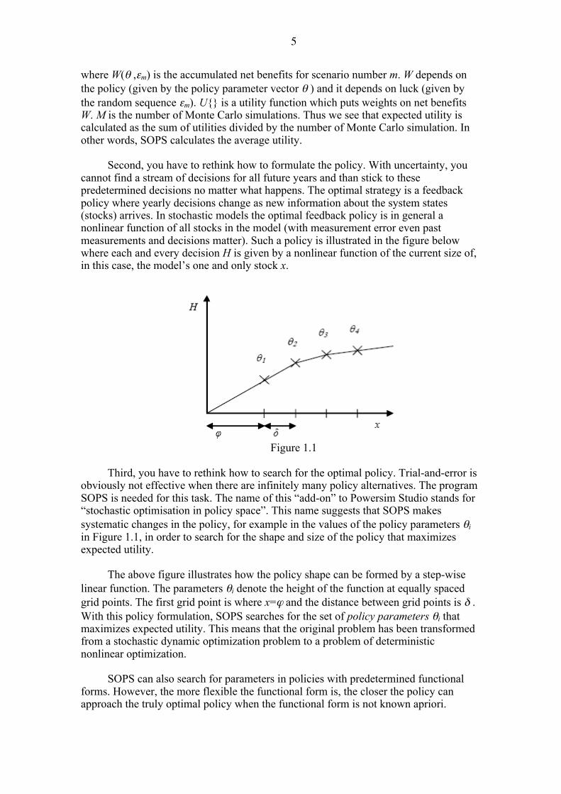
cannot find a stream of decisions for all future years and than stick to these predetermined decisions no matter what happens. The optimal strategy is a feedback policy where yearly decisions change as new information about the system states (stocks) arrives. In stochastic models the optimal feedback policy is in general a nonlinear function of all stocks in the model (with measurement error even past measurements and decisions matter). Such a policy is illustrated in the figure below where each and every decision H is given by a nonlinear function of the current size of, in this case, the model’s one and only stock x.

Figure 1.1

Third, you have to rethink how to search for the optimal policy. Trial-and-error is

obviously not effective when there are infinitely many policy alternatives. The program SOPS is needed for this task. The name of this “add-on” to Powersim Studio stands for “stochastic optimisation in policy space”. This name suggests that SOPS makes systematic changes in the policy, for example in the values of the policy parameters θi in Figure 1.1, in order to search for the shape and size of the policy that maximizes expected utility.

The above figure illustrates how the policy shape can be formed by a step-wise

linear function. The parameters θi denote the height of the function at equally spaced grid points. The first grid point is where x=ϕ and the distance between grid points is δ . With this policy formulation, SOPS searches for the set of policy parameters θi that maximizes expected utility. This means that the original problem has been transformed from a stochastic dynamic optimization problem to a problem of deterministic nonlinear optimization.

SOPS can also search for parameters in policies with predetermined functional

forms. However, the more flexible the functional form is, the closer the policy can approach the truly optimal policy when the functional form is not known apriori.

6

The idea behind optimization in policy space is old and one may also say old fashioned. However with today’s computational power of computers, optimization in policy space provides a simple and efficient alternative. Similar techniques are now used in for instance reinforcement learning.

According to the literature on diffusion of new technologies, simplicity is

important for people to start using new methods. The combination of Studio and SOPS appears to be intuitively appealing. The model is formulated and tested in Studio, testing that any model used for optimization should be subjected to. A mouse click brings you from Studio to SOPS where you make assumptions about stochasticity and initial values of policy parameters, where you choose search method and set parameters for desired accuracy. The resulting policies are easily transferred to other programs for analysis, to produce graphics and for storage.

SOPS simplifies the problem of stochastic optimization in several ways. First,

compared to everyday decision making, the intermediate step of making forecasts is removed. This is possible since forecasts are based on the same variables as policies. Second, compared to stochastic dynamics programming (SDP), the intermediate step of producing a transition matrix from the underlying simulation model is removed. SOPS make direct use of the simulation model. Third, compared to methods to find optimal policies in systems with nonlinearities and measurement error, imperfect state estimation with for instance Kalman filters can be removed. SOPS allows for policies that depend directly on current and past measurements.

B.C. Lubow, in his article “SDP: Generalized software for solving stochastic

dynamic optimization problems.” in Wildlife Society Bulletin 23(4):738-742, 1995, describes the complexity of traditional SDP in the following way: “Undoubtedly, the highly theoretical and mathematical nature of some literature on dynamic programming has also impeded application of this technique (see the discussion of this problem in Nemhauser [1966:245]). However, the absence of adequate software may pose the most significant obstacle facing potential users of the dynamic programming technique.” Lubow goes on to describe his own user friendly package (called SDP), however noting that: “it can not replace user's understanding of the conceptual basis of the technique ---. SDP should not be viewed as a means of providing novices with an easy recipe for solving complex dynamic optimisation problems. Rather, it is intended to assist investigators familiar with dynamic programming ---”.

Hopefully, SOPS represents yet another step in the direction of user friendliness

in that familiarity with dynamic programming is not a prerequisite. This seems important in order to stimulate more widespread analysis of difficult problems that are plagued by nonlinearity, dynamics, stochasticity, measurement error, and uncertainty. Optimal policies under such conditions can at times give very different decisions from those suggested by simple intuition.

To date, most efforts to find optimal policies to complex, stochastic, dynamic

problems have relied on the use of highly simplified models. While these efforts give exact knowledge about the optimal policies for these simplified models, they are not necessarily very helpful for real problems that are more complex. Different from SDP, SOPS can also be used to find near-to-optimal policies for complex models. However, in this case it may be necessary to simplify the policy functions to reduce the number of policy parameters. While SOPS helps increase expected utility in such cases, it does not guarantee that the optimal solution will been found. Since in real life one is competing

7

with decision makers’ judgments and not with ideal solutions, improvement can be highly beneficial.

Similar to SDP, SOPS suffers from the “curse of dimensionality” when using grid

functions. For example if the policy for decision H depends on 5 stock variables, the number of policy parameters will equal the number of grid points in each direction raised to the power of 5. With 10 grid points in each direction, the number of policy parameters will be 105 or one hundred thousand. Compared to SDP which uses discontinuous discretized policies, SOPS benefits somewhat from its continuous piece-wise linear policies. Furthermore, and perhaps surprisingly, the distance between grid points can be increased when measurement error and model error is introduced because these uncertainties seem to lead to smoother policy surfaces. These benefits can not be easily reaped by SDP where measurement error and model error causes great difficulties.

SDP, at least for simple problems, can guarantee that global optima have been

found. Using SOPS, the probability that a global optimum has been found increases with repeated policy searches starting from different sets of initial policy parameters. To reduce uncertainty and to gain confidence in solutions found by SOPS, it may be a good idea to first replicate solutions to simplified models found by SDP, before model complexity is increased.

The following publications give more information about the use of SOPS: - Measurement error and stochasticity are discussed in Moxnes, E. (2003):

“Uncertain measurements of renewable resources: Approximations, harvest policies, and value of accuracy.” Journal of Environmental Economics and Management 45(1):85-108, and in Moxnes, E. (2009): “Complexities in fisheries management: misperceptions and communication.” in Handbook of Marine Fisheries Conservation and Management, edited by Hilborn, R., Squires, D., Williams, M., Tait, M., and Grafton, Q. Oxford: Oxford University Press.

- Model error is assumed in Moxnes, E. (2007). “Guidelines for the analysis of complex, dynamic systems (The unavoidable a priori revisited, or deriving the principles of SD).” in proceedings of the International System Dynamics Conference. Boston: System Dynamics Society.

- Policy sensitivity is discussed in Moxnes, E. (2005). “Policy Sensitivity Analysis: simple versus complex fishery models.” System Dynamics Review 21(2):123-145.

- In the future, SOPS may be improved by methods to test the goodness of policy approximation, see Moxnes, E. (1998). “Catch policy for a predator-prey system: measurement error and value of accuracy.” Report No. 56/98. Bergen: SNF. In the future, the program could also be transferred to much more powerful parallel computers (Monte-Carlo simulations are particularly well suited for parallel computing).

8

2. MODELLING WITH POWERSIM STUDIO

This chapter is not likely to contain all the information you need to model and simulate with Powersim Studio. Studio’s help function should be used for more detailed questions. For an introduction to modelling, see Sterman, J.D. (2000): Business Dynamics, Irwin/McGraw-Hill, Boston. Here we only indicate the fundamentals of particular importance for optimizing with SOPS. The next chapter explains the special policy functions in Studio that are needed to run SOPS. Thus, experienced users of Studio can skip to the next chapter, although they may benefit from the discussion of discrete time models in Section 2.1 of this chapter.

2.1. Modelling

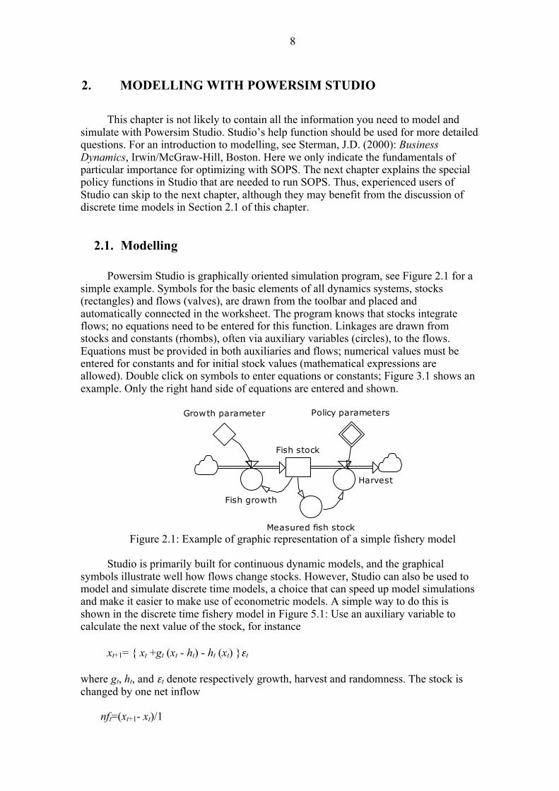
Powersim Studio is graphically oriented simulation program, see Figure 2.1 for a simple example. Symbols for the basic elements of all dynamics systems, stocks (rectangles) and flows (valves), are drawn from the toolbar and placed and automatically connected in the worksheet. The program knows that stocks integrate flows; no equations need to be entered for this function. Linkages are drawn from stocks and constants (rhombs), often via auxiliary variables (circles), to the flows. Equations must be provided in both auxiliaries and flows; numerical values must be entered for constants and for initial stock values (mathematical expressions are allowed). Double click on symbols to enter equations or constants; Figure 3.1 shows an example. Only the right hand side of equations are entered and shown.

Fish stock

Fish growth

Harvest

Policy parametersGrowth parameter

Measured fish stock Figure 2.1: Example of graphic representation of a simple fishery model

Studio is primarily built for continuous dynamic models, and the graphical

symbols illustrate well how flows change stocks. However, Studio can also be used to model and simulate discrete time models, a choice that can speed up model simulations and make it easier to make use of econometric models. A simple way to do this is shown in the discrete time fishery model in Figure 5.1: Use an auxiliary variable to calculate the next value of the stock, for instance

xt+1= { xt +gt (xt - ht) - ht (xt) }εt

where gt, ht, and εt denote respectively growth, harvest and randomness. The stock is changed by one net inflow nft=(xt+1- xt)/1

9

where the time step is 1 time unit. Graphically this discrete representation does not give a good illustration of how stocks change through in- and outflows.

2.2. Simulating

Once the model is formulated without error messages, it takes only a mouse click to simulate it. Results can be shown in tables and graphs. Select the symbols from the toolbar and paste them in the worksheet. Drag variables into the tables or graphs.

2.3. Beginner’s hints for Powersim Studio

In this section we give some advice to prevent some problems that beginners often struggle with.

First time start-up Choose New on the File menu. Click Next, choose language and mark Use as

default. Next, do NOT mark Studio 2005 file format compatibility, mark Use as default. Next, mark Calendar-independent simulation. Next, fill in time unit (e.g. year) and Time unit as interval (e.g. years). Later on, when you start a new project, choose New on the File menu.

Normal and Advanced toolbar For normal simulations it is sufficient to use a reduced toolbar set. Choose:

View>Workspace>Restore User Interface>Normal (as opposed to Advanced). However, before transferring to SOPS, you have to choose the Advanced toolbar!

Time unit and time steps

To change the time unit, click on the hammer/wrench button in the toolbar and choose Time measurement. Always choose calendar-independent simulations! If Enforce time unit consistency is turned on, you have to specify what the time unit is, and you have to specify the time unit in all constants where it is appropriate, for instance 2.4<<year>> or 3.5/1<<year>>. Remember, all flows must be per unit of time. You may turn off the Enforce time unit consistency, in which case you do not need to represent time units.

To set the simulation time step as well as start and stop times, choose

Simulation>Simulation Settings. Note that Studio operates with different units for points in time and time intervals. Points in time use the prefix @, for instance <<@year>>. The predefined Studio variable TIME denotes points in time. Thus in expressions that require a time interval as input, you must subtract another point in time, for instance TIME-STARTTIME.

Other units than for time

10

You can choose whether you want to use units or not. This can simply be done by not assigning units to your constants and initial stock values (but you have to be consistent!). Units follow numerical values, for instance 6.6<<meter>>. When entering a unit that has not been used before in your model, you will see in red the following text: “The name ‘meter’ is unknown”. Click the OK button and you get the chance to create meter as a global unit. Next time you need this unit you may first click the radio button for Units and then find your global unit in the list of units. Point your cursor to the appropriate place in the expression and double click on the unit. You may also type in the unit. Check that Auto is marked and do not touch the drop-down menu to the right of the Auto mark unless you really know what you are doing.

Auxiliaries and flows will automatically get the units that follow from the

constants, stocks and other auxiliaries that are entered into the equations. Again check that Auto is marked. You may, if you wish, enter constants with their units directly into auxiliary and flow equations (e.g. x/2.2<<meter>>). Such constants cannot be changed after you have transferred to SOPS.

Reporting intervals in tables and figures To change the reporting interval in tables: double-click on the border of the table,

choose the tab General, and specify the desired report interval. In graphs you double-click on the x-axis and change the interval.

Hiding constants and showing constants in shared diagrams To make the symbol for a constant disappear in the shared diagrams, right click

on the symbol and choose Exclude Variable. To make it reappear first move to the equations diagram (find symbol in the toolbar). Then you right click on the variable in the equations diagram, hold the mouse button down, and drag the constant into the line named Shared Diagrams to the very left (you have to be in Advanced View to see list of windows to the left). This makes the window shift from equations to shared diagrams view. Still holding the button down; drag the constant symbol into the shared diagram to its desired position. Add the lacking linkages.

11

3. SOPS POLICY FUNCTIONS

There are two types of functions that SOPS recognizes as policy functions. These functions have policy parameters θ that SOPS recognizes and changes in order to maximize expected utility. The two types are flexible grid policies and pre-specified functional forms referred to as custom policies. Note that in addition to the policy functions with searchable parameters θ, you can specify fixed logical constraints on any policy. The most typical constraint is to limit policies to positive numbers. This is done by a separate max-function which takes its input from the policy function variable.

3.1. Grid policy functions

There are two types of grid functions available, the second of which gives the user more freedom to explore policies within the SOPS program.

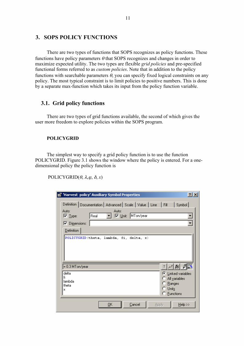
POLICYGRID The simplest way to specify a grid policy function is to use the function

POLICYGRID. Figure 3.1 shows the window where the policy is entered. For a one-dimensional policy the policy function is

POLICYGRID(θ, λ,ϕ, δ, x)

12

Figure 3.1: Studio window for specification of equations or constants. Figure 3.2 shows how the policy parameter vector θ is defined. First note that all

policy parameters are defined as permanent constants. To set a constant as permanent, choose the tag Advanced; the tag can be seen in figure. Tick off for permanent. Since θ is a vector with many values, you have to specify the dimension. With for example 4 policy parameters, the dimension is denoted 1..4. Values are written in a parenthesis {} followed by the appropriate unit.

Figure 3.2: Specification of initial policy parameter values

The next parameter vector is λ which denotes a lower and an upper limit for the

policy. Since there are two limits, the dimension is denoted 1..2. The unit is the same as for θ. The main purpose of these limits is to prevent episodes where the search routine moves into unreasonable ranges. Normally one can choose wide ranges. If this option is used to set logical limits on the policy, that may reduce accuracy as it forces the policy to reach limits exactly at grid points. It is better to use for instance a max-function in a subsequent auxiliary variable.

The next two parameters, first grid point ϕ and step size δ, are defined in Figure

3.3 and determine the grid structure. Both grid parameters have the same unit as x. Finally, x is the input variable that influences decisions through the policy function.

13

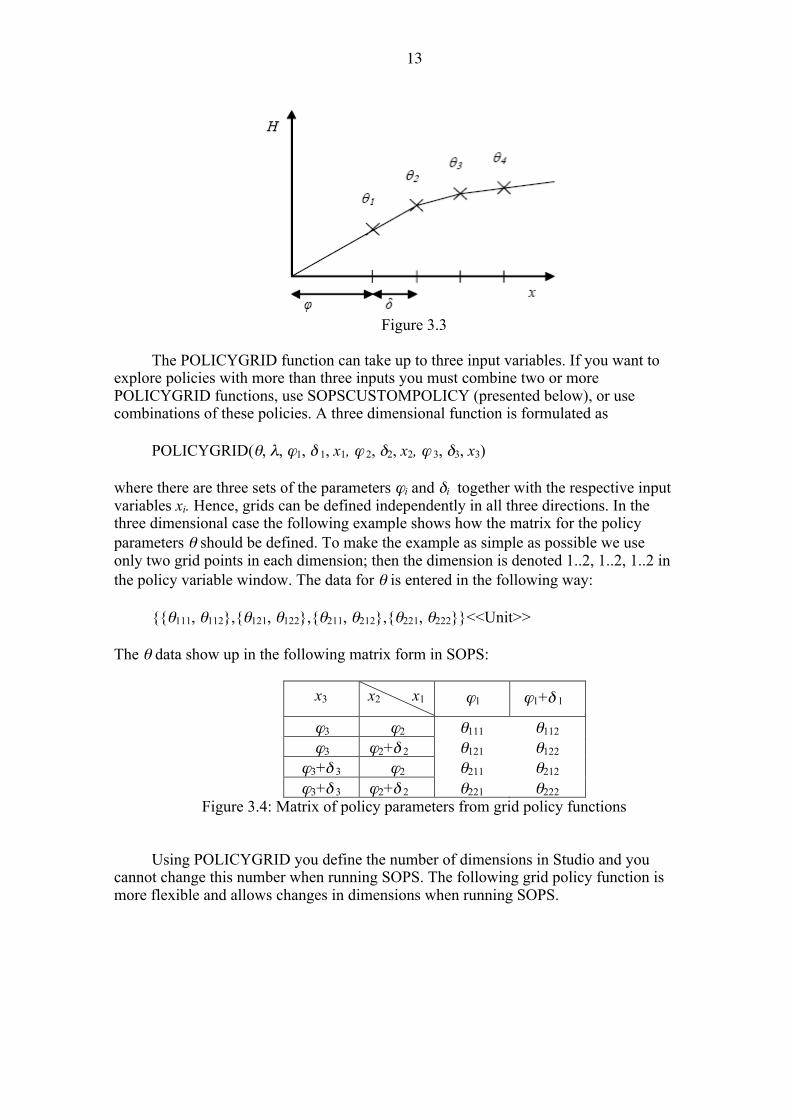
Figure 3.3

The POLICYGRID function can take up to three input variables. If you want to

explore policies with more than three inputs you must combine two or more POLICYGRID functions, use SOPSCUSTOMPOLICY (presented below), or use combinations of these policies. A three dimensional function is formulated as

POLICYGRID(θ, λ, ϕ1, δ 1, x1, ϕ 2, δ2, x2, ϕ 3, δ3, x3)

where there are three sets of the parameters ϕi and δi together with the respective input variables xi. Hence, grids can be defined independently in all three directions. In the three dimensional case the following example shows how the matrix for the policy parameters θ should be defined. To make the example as simple as possible we use only two grid points in each dimension; then the dimension is denoted 1..2, 1..2, 1..2 in the policy variable window. The data for θ is entered in the following way:

{{θ111, θ112},{θ121, θ122},{θ211, θ212},{θ221, θ222}}<<Unit>>

The θ data show up in the following matrix form in SOPS:

x3 x2 x1 ϕ1 ϕ1+δ 1

ϕ3 ϕ2 θ111 θ112

ϕ3 ϕ2+δ 2 θ121 θ122 ϕ3+δ 3 ϕ2 θ211 θ212 ϕ3+δ 3 ϕ2+δ 2 θ221 θ222

Figure 3.4: Matrix of policy parameters from grid policy functions

Using POLICYGRID you define the number of dimensions in Studio and you

cannot change this number when running SOPS. The following grid policy function is more flexible and allows changes in dimensions when running SOPS.

14

SOPSPOLICYGRID Here the SOPSPOLICYGRID function is shown for the case with three

dimensions (which is the maximum number of dimensions in the current version of SOPS):

SOPSPOLICYGRID(θ, ρ, λ, ϕ1, δ 1, x1, ϕ 2, δ2, x2, ϕ 3, δ3, x3) The difference from POLICYGRID is that θ is given in a sequential form

(without parentheses) and it is followed by a vector of integers ρ denoting the initial number of grid points in each dimension. To get the same result as in the above three dimensional example for POLICYGRID, data for θ must be entered in the following way:

{θ111, θ112, θ121, θ122, θ211, θ212, θ221, θ222}<<Unit>>

and data for ρ (integer, no unit, and dimension 1..3) must be entered as: { 2, 2, 2 } Figure 3.4 also illustrates how this θ matrix shows up in SOPS.

Note that when running SOPS, you are free to choose any combination of integers in the ρ-vector, provided the total number of policy parameters does not exceed the initial number, in the example 2∗2∗2=8. If an element in ρ is set equal to zero, the input variable for that dimension will not be considered. In this example one of the other two input variables could have four grid points.

3.1. Custom policies

SOPSCUSTOMPOLICY

This policy function allows the user to pre-specify the functional form. While this

does allow for great variation in functional forms, pre-specified functions will in general restrict the solution and prevent that you find truly optimal solutions. The only exception is when you have happened to choose a correct functional form. The main benefit of customized policies is that the number of policy parameters can be kept at a low level. The following example illustrates:

SOPSCUSTOMPOLICY(α0+ α1x1+ α2x2+ α3x3+ α4x4+......) Remember that also policy parameters in the SOPSCUSTOMPOLICY must be

defined as permanent constants! In this example only one policy parameter αi is used for each dimension. This restricts the solution to a hyper plane which for instance could be restricted to positive policy values by a subsequent MAX-function. While this policy is not likely to be the optimal one for most nonlinear models, it may help indicate which dimensions are most important to capture in ensuing tests of grid functions.

15

You will have problems finding optimal solutions if the terms in

SOPSCUSTOMPOLICY are strongly correlated (similar to the problem of multicolinearity in statistics). The simplest example to illustrate this problem is the policy function y=ax+bx where the two explanatory variables are exactly the same. While a+b could be determined, it is impossible to determine individual values for a and b. Therefore one should avoid information sources that are strongly correlated, for instance if x1 represents a short information delay of x2. A first question then is if it is really necessary to represent both variables in the model. If the answer is yes, a solution could be to use the difference between the two variables as the second variable.

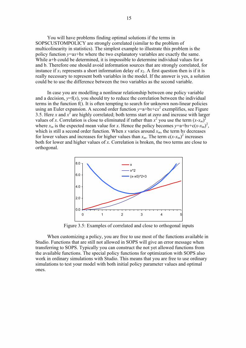
In case you are modelling a nonlinear relationship between one policy variable

and a decision, y=f(x), you should try to reduce the correlation between the individual terms in the function f(). It is often tempting to search for unknown non-linear policies using an Euler expansion. A second order function y=a+bx+cx2 exemplifies, see Figure 3.5. Here x and x2 are highly correlated; both terms start at zero and increase with larger values of x. Correlation is close to eliminated if rather than x2 you use the term (x-xm)2 where xm is the expected mean value for x. Hence the policy becomes y=a+bx+c(x-xm)2, which is still a second order function. When x varies around xm, the term bx decreases for lower values and increases for higher values than xm. The term c(x-xm)2 increases both for lower and higher values of x. Correlation is broken, the two terms are close to orthogonal.

0.0

2.0

4.0

6.0

8.0

0 1 2 3 4 5

x

x^2

(x-x0)^2+3

Figure 3.5: Examples of correlated and close to orthogonal inputs

When customizing a policy, you are free to use most of the functions available in Studio. Functions that are still not allowed in SOPS will give an error message when transferring to SOPS. Typically you can construct the not yet allowed functions from the available functions. The special policy functions for optimization with SOPS also work in ordinary simulations with Studio. This means that you are free to use ordinary simulations to test your model with both initial policy parameter values and optimal ones.

16

4. TRANSFERRING FROM STUDIO TO SOPS

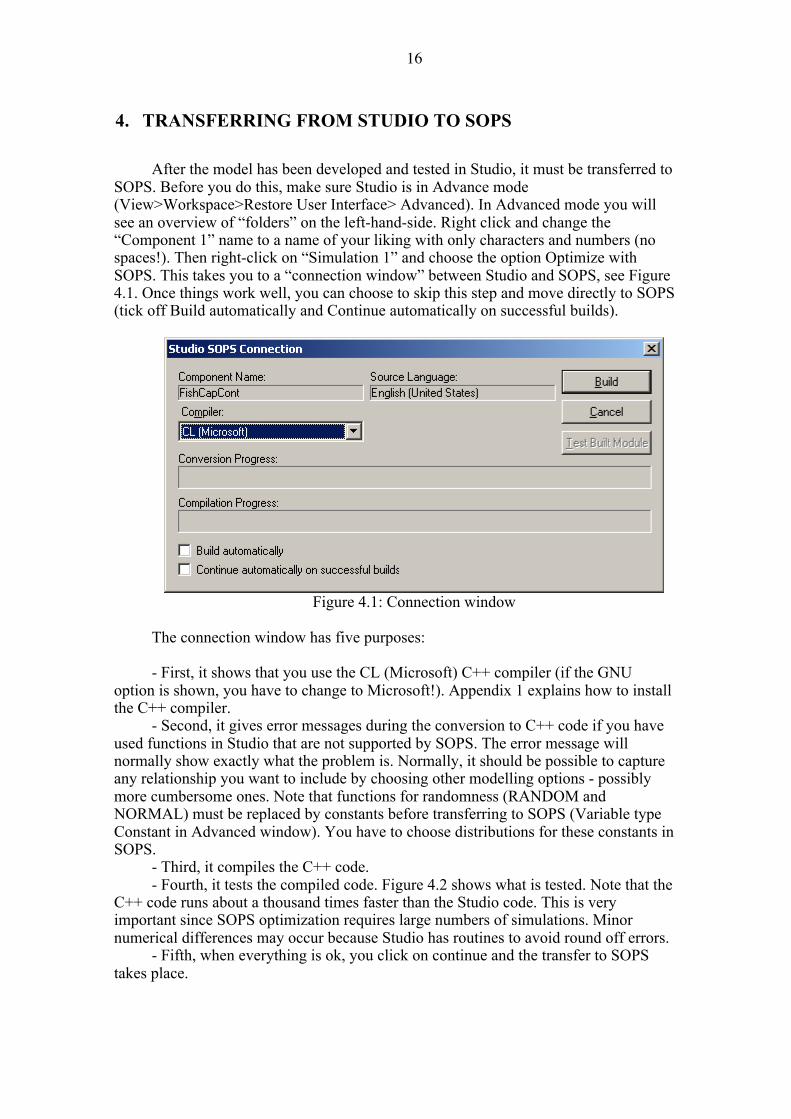
After the model has been developed and tested in Studio, it must be transferred to SOPS. Before you do this, make sure Studio is in Advance mode (View>Workspace>Restore User Interface> Advanced). In Advanced mode you will see an overview of “folders” on the left-hand-side. Right click and change the “Component 1” name to a name of your liking with only characters and numbers (no spaces!). Then right-click on “Simulation 1” and choose the option Optimize with SOPS. This takes you to a “connection window” between Studio and SOPS, see Figure 4.1. Once things work well, you can choose to skip this step and move directly to SOPS (tick off Build automatically and Continue automatically on successful builds).

Figure 4.1: Connection window

The connection window has five purposes: - First, it shows that you use the CL (Microsoft) C++ compiler (if the GNU

option is shown, you have to change to Microsoft!). Appendix 1 explains how to install the C++ compiler.

- Second, it gives error messages during the conversion to C++ code if you have used functions in Studio that are not supported by SOPS. The error message will normally show exactly what the problem is. Normally, it should be possible to capture any relationship you want to include by choosing other modelling options - possibly more cumbersome ones. Note that functions for randomness (RANDOM and NORMAL) must be replaced by constants before transferring to SOPS (Variable type Constant in Advanced window). You have to choose distributions for these constants in SOPS.

- Third, it compiles the C++ code. - Fourth, it tests the compiled code. Figure 4.2 shows what is tested. Note that the

C++ code runs about a thousand times faster than the Studio code. This is very important since SOPS optimization requires large numbers of simulations. Minor numerical differences may occur because Studio has routines to avoid round off errors.

- Fifth, when everything is ok, you click on continue and the transfer to SOPS takes place.

17

Figure 4.2: Simulation test of compiled C++ code

After changes in the simulation model it may be necessary to delete existing .sops

file before you compile the model again. The .sops files may contain information related to previous model versions.

18

5. OPTIMIZING WITH SOPS

In this introduction we use two example models to introduce SOPS. The first model is in discrete time and uses SOPSCUSTOMPOLICY functions. The second is formulated as a continuous time model and uses POLICYGRID and SOPSPOLICYGRID functions.

To focus on policy functions, the Studio diagrams show all policy parameter

symbols while model constants are hidden and can only be seen in equations view. For normal purposes it is better to hide the many policy parameter symbols to simplify the graphics. Both models are available as downloads for Studio. If you have installed the SOPS program but have not installed Studio, you can download compiled versions of the two models to test how SOPS works, see Appendix 1.

Studio models are stored with the post script .sip. SOPS operates with three

different types of files. The compiled model has the post script .csim. Model assumptions and results are stored with the post script .sops. For each .csim model you can store many .sops files using different names for different assumptions and related results. You may activate the stored assumptions and results by either double clicking on the .sops files or open the preferred file under File>Open when running the corresponding .csim model. The result.txt file contains error messages for program developers and is not required when running SOPS.

5.1. Discrete time model and custom policies The example fishery model is shown in Figure 5.1. The challenge is to find a

harvesting policy and a capacity policy that yields the highest possible expected net present value for the fishery. For a fixed discount rate, the future value is proportional to the present value (=future value/(1+discount rate)T), where T is the time horizon. Thus it does not matter whether one maximizes the future or the present value. Here we choose the standard net present value expression.

The discount rate implies that the first years of the simulation weigh more than

the later years. Low weights on future years mean that an infinite horizon can be approximated by a limited number of time periods. In practise it may also work well to perform optimization with a discount rate of zero. A sufficiently long time horizon to ensure no further changes in policy functions can be found by trial-and-error.

The exact formulations in the model can be seen in equations view of the

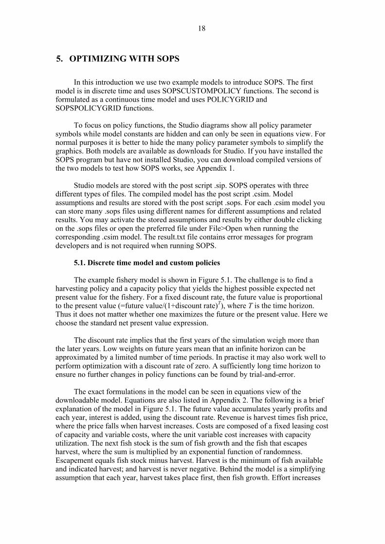
downloadable model. Equations are also listed in Appendix 2. The following is a brief explanation of the model in Figure 5.1. The future value accumulates yearly profits and each year, interest is added, using the discount rate. Revenue is harvest times fish price, where the price falls when harvest increases. Costs are composed of a fixed leasing cost of capacity and variable costs, where the unit variable cost increases with capacity utilization. The next fish stock is the sum of fish growth and the fish that escapes harvest, where the sum is multiplied by an exponential function of randomness. Escapement equals fish stock minus harvest. Harvest is the minimum of fish available and indicated harvest; and harvest is never negative. Behind the model is a simplifying assumption that each year, harvest takes place first, then fish growth. Effort increases

19

with harvest and it decreases with the fish stock (lower effort with higher density of fish).

future value

interest

profits

costs

revenue

fish stock

fish price

effort

escapement

ind harvest

harvest

Next fish stock

update

present value

randomness

utilizationunit variable costcap const

a0 a1 a2

fish stock ref

ind investment

cap slope fish

capacity varinvestment depreciation

cap slope cap

capacity

sw

const capacity

harv cap

cap ref

ind capacity

Figure 5.1: Discrete time model with custom policies The policy for indicated harvest is: SOPSCUSTOMPOLICY(a0+a1*'fish stock' + a2*('fish stock'-'fish stock ref')^2 +

'harv cap'*(capacity-'cap ref'))

where 'fish stock ref'’=2 Mton is a guess of the mean value of the fish stock with an optimal policy in place (does not have to be very accurate and could be changed by manual iteration). This term removes most of the correlation between the second and third term that would result with 'fish stock ref'’=0, see Figure 3.5. The last term allows for adjustments of harvest due to changes in capacity. Here 'cap ref'=0.4 Mton/year is a guess of the optimal capacity. This parameter is not important for the effectiveness of the optimization routine but may be helpful when guessing about initial policy parameters.

There are two alternative policies for capacity, either capacity is constant where indicated capacity is simply given as:

SOPSCUSTOMPOLICY('const capacity'). Or, capacity varies over time. In this case the average lifetime of capacity is 15

years and indicated investments are given as

20

SOPSCUSTOMPOLICY('cap const' + 'cap slope fish' * ('fish stock'-2<<MTon>>) + 'cap slope cap' * ('capacity var'-0.4<<MTon/year>>))

Here we have inserted numerical values for 'fish stock ref' and 'cap ref'. Note that

doing it this way makes it impossible to change values while running SOPS. Max-functions in subsequent variables ensure that investments and capacity do not go negative. The constant sw can be set to 0 or 1 in SOPS to switch between variable and constant capacity, a quick way to change model structure when running SOPS. The equation for capacity is:

MAX(0<<MTon/year>>, 'ind capacity' * sw + (1-sw) * 'capacity var')

Figure 5.2 shows the first page in SOPS with tags for the five other pages. The

page can be resized by dragging the lower right corner. As an alternative to using the mouse, you can move around using arrows and by typing Alt-letter. Starting from below, you see the time horizon for the simulations, 50 years. The value comes from the original Studio model. However, you are free to change its value in SOPS. The time step is 1 unit, which you should not change when dealing with a discrete time model. Next, you can choose between Monte Carlo and Latin Hypercube simulations. In this example there are only minor differences with respect to speed and accuracy, and we choose the default choice: Monte Carlo. Notice that the two methods give slightly different criterion values since the two methods produce slightly different scenarios of future randomness.

Figure 5.2: Page 1 - General Settings

21

You determine how many simulated futures you want (the simulation count). Options range from 1 to 10000. You determine how frequently random variables should change. In this discrete time model you should not deviate from the model time step of 1 time unit. You can also choose the seed for the simulations, which gives you an alternative set of possible futures. Note that for every optimization, SOPS operates with the same set of simulated futures. Hence there is no difference from search to search; each search should ideally result in the same policy parameters and the same criterion value.

You have a choice of two optimization methods: the gradient method and an

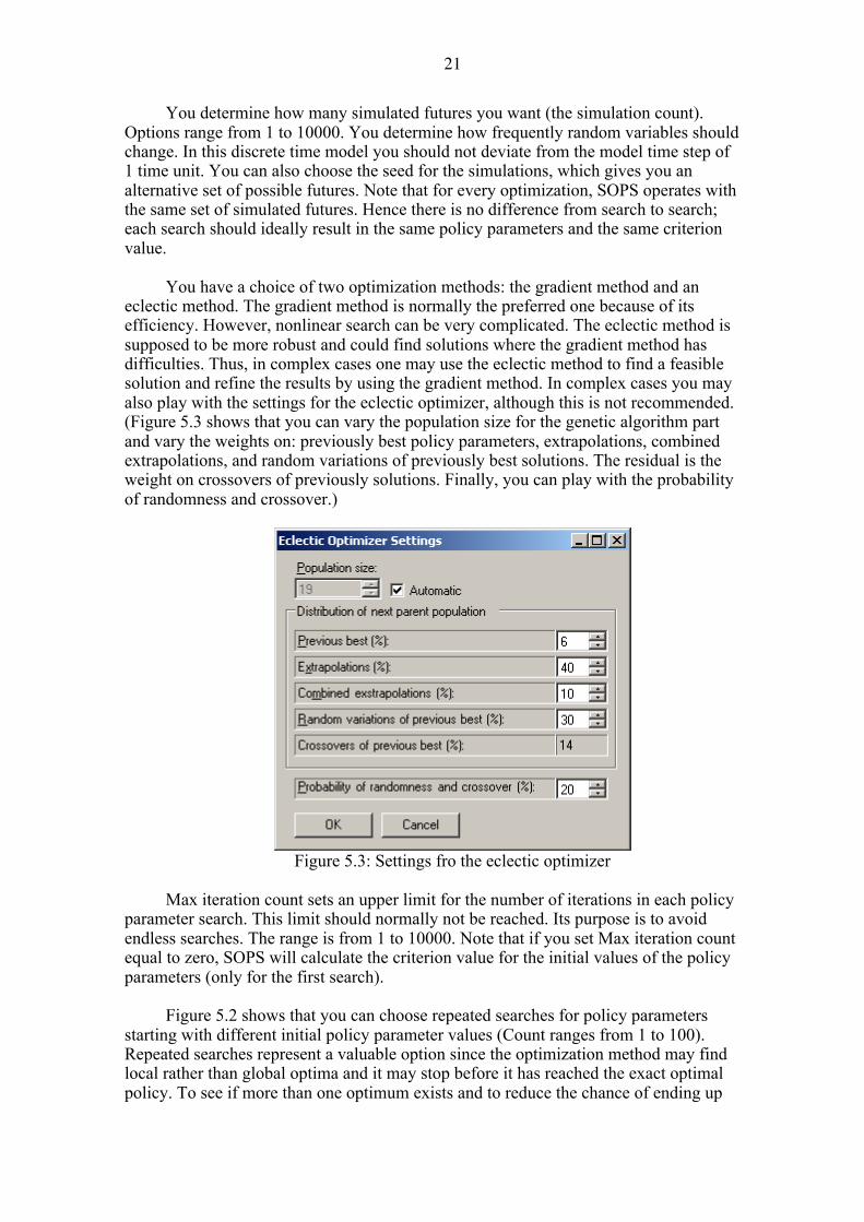
eclectic method. The gradient method is normally the preferred one because of its efficiency. However, nonlinear search can be very complicated. The eclectic method is supposed to be more robust and could find solutions where the gradient method has difficulties. Thus, in complex cases one may use the eclectic method to find a feasible solution and refine the results by using the gradient method. In complex cases you may also play with the settings for the eclectic optimizer, although this is not recommended. (Figure 5.3 shows that you can vary the population size for the genetic algorithm part and vary the weights on: previously best policy parameters, extrapolations, combined extrapolations, and random variations of previously best solutions. The residual is the weight on crossovers of previously solutions. Finally, you can play with the probability of randomness and crossover.)

Figure 5.3: Settings fro the eclectic optimizer

Max iteration count sets an upper limit for the number of iterations in each policy

parameter search. This limit should normally not be reached. Its purpose is to avoid endless searches. The range is from 1 to 10000. Note that if you set Max iteration count equal to zero, SOPS will calculate the criterion value for the initial values of the policy parameters (only for the first search).

Figure 5.2 shows that you can choose repeated searches for policy parameters

starting with different initial policy parameter values (Count ranges from 1 to 100). Repeated searches represent a valuable option since the optimization method may find local rather than global optima and it may stop before it has reached the exact optimal policy. To see if more than one optimum exists and to reduce the chance of ending up

22

with a local optimum or an imprecise results, repeated searches are made from different initial policy parameter values chosen randomly. You can change the seed for random variations in initial policy parameters. As will be seen later, initial policy parameters can also be changed manually.

Figure 5.4 shows page 2 for Assumptions. On the left hand side are symbols for

all constants and initial stock values in the Studio model. Click on one of the candidates. It shows up under Assumptions and the original symbol becomes grey. If you want to deactivate it again, remove the tick. NOTE: Do NOT click on policy parameters under Assumptions. If you enter a policy parameter, and even if you deactivate it again, the value you set in page 2 will override the initial policy parameter values that shall be set in pages 3 and 4.

Under Sampling you can choose between settings for Initial values or time Series.

For initial stock values and parameters that do not change over time, choose Initial. For random variables that change over time, choose Series. The Series-example in Figure 5.4 is randomness, which had to be a constant in the Studio model. Under Type, you can choose type of variation; the mini-window shows the alternatives. Either the parameter has a fixed value or it varies randomly with a choice between the following distributions: exponential, normal, triangular, truncated normal, and uniform. Here we choose normal for randomness.

Figure 5.4: Page 2 - Assumptions

23

The choice you make regarding Type determines what options you have under Value. The figure shows that fixed values require only one number, while the normal distribution asks for both expected value and standard deviation. NOTE: It is ONLY random variables (Series) that are influenced by the tick mark. Initial values will keep the chosen values independent of the tick mark.

The option to change values of model parameters allows for considerable

experimentation inside SOPS. The “switch constant” sw illustrates. Setting it to sw=1 makes the model choose a constant capacity; sw=0 selects variable capacity. This allows you to test different policies in this case and in general, the sensitivity of policies to different model assumptions. We first choose sw=1 to test a policy with constant capacity.

For the discrete time model we skip page 3 for Grid Policies and move on to page 4

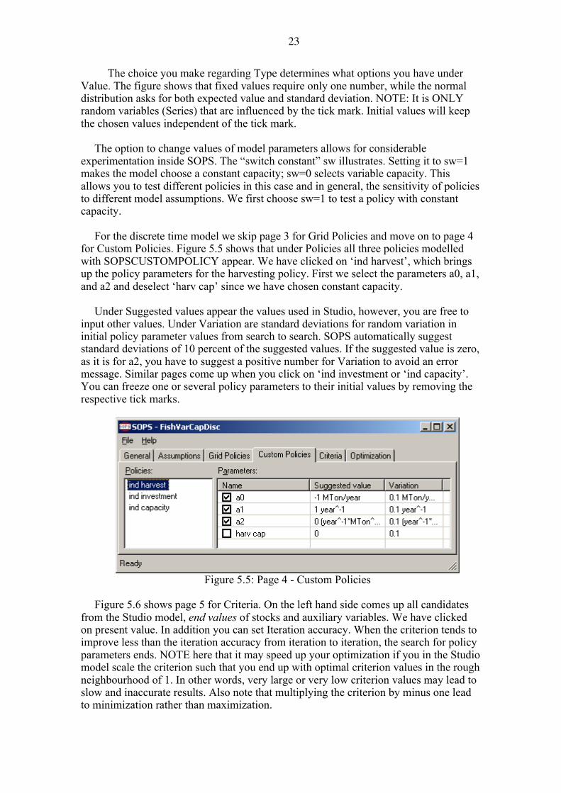
for Custom Policies. Figure 5.5 shows that under Policies all three policies modelled with SOPSCUSTOMPOLICY appear. We have clicked on ‘ind harvest’, which brings up the policy parameters for the harvesting policy. First we select the parameters a0, a1, and a2 and deselect ‘harv cap’ since we have chosen constant capacity.

Under Suggested values appear the values used in Studio, however, you are free to

input other values. Under Variation are standard deviations for random variation in initial policy parameter values from search to search. SOPS automatically suggest standard deviations of 10 percent of the suggested values. If the suggested value is zero, as it is for a2, you have to suggest a positive number for Variation to avoid an error message. Similar pages come up when you click on ‘ind investment or ‘ind capacity’. You can freeze one or several policy parameters to their initial values by removing the respective tick marks.

Figure 5.5: Page 4 - Custom Policies

Figure 5.6 shows page 5 for Criteria. On the left hand side comes up all candidates

from the Studio model, end values of stocks and auxiliary variables. We have clicked on present value. In addition you can set Iteration accuracy. When the criterion tends to improve less than the iteration accuracy from iteration to iteration, the search for policy parameters ends. NOTE here that it may speed up your optimization if you in the Studio model scale the criterion such that you end up with optimal criterion values in the rough neighbourhood of 1. In other words, very large or very low criterion values may lead to slow and inaccurate results. Also note that multiplying the criterion by minus one lead to minimization rather than maximization.

24

Figure 5.6: Page 5 - Criteria

Figure 5.7 shows page 6 for Optimization. In this example optimization has started

but is not yet finished. Progress is shown in terms of number of searches; in the example 2 out of 5 searches have been completed. Progress is also shown in terms of accumulated Simulations, here 143500. Iteration refers to number of iterations in the ongoing search (the third), and the current Criterion value for this search is 53.974....MrdNOK.

Figure 5.7: Page 6 - Optimization - Running

Under the headline Temporary results, while optimization is going on, you can select

and see the criterion values for the finished searches and the corresponding policy parameter values. You have to select which policy you want to examine. In Figure 5.7

25

the harvest policy is shown (‘ind harvest’), capacity policies (‘ind capacity’ and ‘ind investments’) do not show until they are chosen.

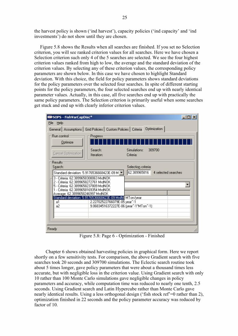
Figure 5.8 shows the Results when all searches are finished. If you set no Selection

criterion, you will see ranked criterion values for all searches. Here we have chosen a Selection criterion such only 4 of the 5 searches are selected. We see the four highest criterion values ranked from high to low, the average and the standard deviation of the criterion values. By selecting any of these criterion values, the corresponding policy parameters are shown below. In this case we have chosen to highlight Standard deviation. With this choice, the field for policy parameters shows standard deviations for the policy parameters over the selected four searches. In spite of different starting points for the policy parameters, the four selected searches end up with nearly identical parameter values. Actually, in this case, all five searches end up with practically the same policy parameters. The Selection criterion is primarily useful when some searches get stuck and end up with clearly inferior criterion values.

Figure 5.8: Page 6 - Optimization - Finished

Chapter 6 shows obtained harvesting policies in graphical form. Here we report shortly on a few sensitivity tests. For comparison, the above Gradient search with five searches took 20 seconds and 309700 simulations. The Eclectic search routine took about 5 times longer, gave policy parameters that were about a thousand times less accurate, but with negligible loss in the criterion value. Using Gradient search with only 10 rather than 100 Monte Carlo simulations gave negligible changes in policy parameters and accuracy, while computation time was reduced to nearly one tenth, 2.5 seconds. Using Gradient search and Latin Hypercube rather than Monte Carlo gave nearly identical results. Using a less orthogonal design (‘fish stock ref’=0 rather than 2), optimization finished in 22 seconds and the policy parameter accuracy was reduced by factor of 10.

26

As a final test of the discrete time model, we relax the assumption of fixed

capacity. Under Assumptions we choose sw=0 rather than 1. Under Custom Policies we activate the policy parameter ‘harv cap’ in the harvesting policy, we deactivate ‘const capactiy’ in the capacity policy, and we activate all three policy parameters in the investment policy.

As will be seen in Chapter 6, we find that harvest should vary with capacity in

addition to fish stock and investments should also vary with both capacity and fish stock. However, the gain in the criterion by allowing capacity to vary is marginal, only 0.26 percent. In the next section we use grid functions which allow for flexible nonlinear policy functions. We will see if our use of simplifying assumptions in terms of SOPSCUSTOMPOLICY and a time discrete model had a major impact on policies.

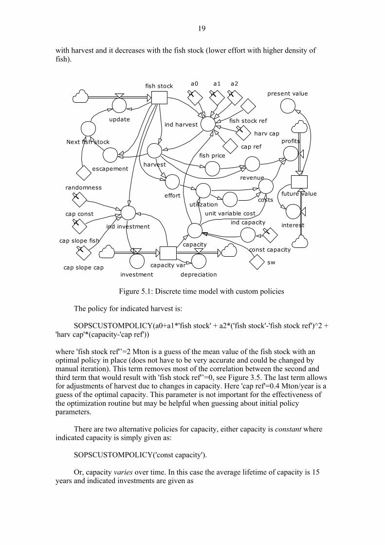
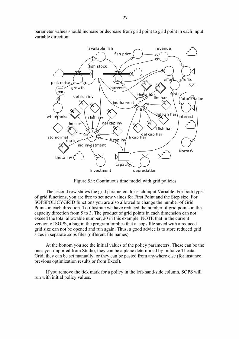
5.2. Continuous time model and grid policies Then we turn to the second fishery model which has a continuous time

representation and where we demonstrate policy grid functions, see Figure 5.9. A nice feature of continuous models is that the diagrams become more intuitive. Stocks increase by inflows and are reduced by outflows; and it is usually easy to establish first order control to avoid that stocks go negative. The latter is more important in stochastic models than in deterministic ones because random future scenarios can create unexpectedly wild behaviour - particularly while policy parameters are still far away from optimal values. Typically the time step for the numerical simulation of continuous type models is shorter than that for discrete time models. The length of the time step must be set short enough to obtain acceptable accuracy.

With a continuous representation, the major differences from the discrete time

model with variable capacity are the following. We no longer need to assume that harvest takes place first and fish growth next. Harvest and growth goes on at the same time. Randomness now applies to fish growth rather than to predicted next period fish stock. Since the time step is much shorter (0.2 year rather than 1.0), we introduce autocorrelation (pink noise). Looking at the exact equations in Appendix 2 one will also see that the expression for effort is much simpler and intuitive in the continuous model. Rather than the present values we use a normalized version of future value such that we end up with criterion values in the neighbourhood of 1.0. Future value is probably intuitively easier to understand than net present value (like a bank account), while it has no consequence for the policy parameters. Similar to the discrete time model, and similar to real decisions on fishing quotas, harvest is updated only once a year.

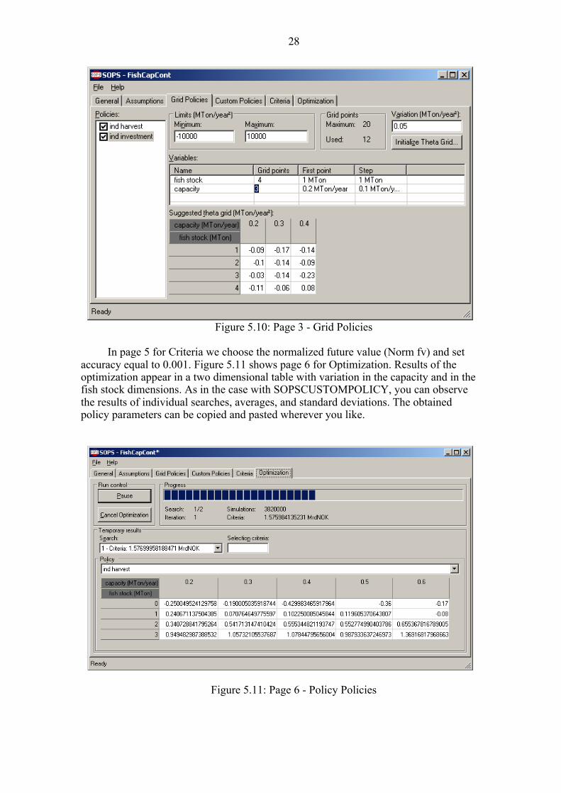
Using grid functions, page 3 for Grid Policies is used to set initial values of the

grid policy functions and to set variation in the individual parameters, see Figure 5.10. Activate the policy you want to change by clicking on its name in the left-hand-side column. Here we activate the policy for harvest, which applies SOPSPOLICYGRID. In the upper row you can set Minimum and Maximum limits for the policy parameters. Under Variation you can set the standard deviation for random variation in initial policy parameters (all parameters for the chosen policy). Zero will lead to an error message. In addition, you can observe the utilization of Grid Points; which is only interesting for the SOPSPOLICYGRID function where you can reduce the number of grid points used in the optimization. In the example, 12 out of 20 grid points are used. Finally, the upper row gives you one of several options to Initialize the Theta Grid. Click on this option and set the value in the upper left corner of the matrix and then enter how much the

27

parameter values should increase or decrease from grid point to grid point in each input variable direction.

future value

interest

profits

costs

revenue

fish stock

fish price

effort

ind harvest

growth

theta harlim har

fi fish har

del fish har

capacityinvestment

ind investment

harvest

depreciation

theta inv

lim invfi fish inv

del fish inv

fi cap inv

del cap inv

fi cap hardel cap har

available fish

std normalrho inv

pink noise

white noise

Norm fv

Figure 5.9: Continuous time model with grid policies

The second row shows the grid parameters for each input Variable. For both types of grid functions, you are free to set new values for First Point and the Step size. For SOPSPOLICYGRID functions you are also allowed to change the number of Grid Points in each direction. To illustrate we have reduced the number of grid points in the capacity direction from 5 to 3. The product of grid points in each dimension can not exceed the total allowable number, 20 in this example. NOTE that in the current version of SOPS, a bug in the program implies that a .sops file saved with a reduced grid size can not be opened and run again. Thus, a good advice is to store reduced grid sizes in separate .sops files (different file names).

At the bottom you see the initial values of the policy parameters. These can be the

ones you imported from Studio, they can be a plane determined by Initiaize Theata Grid, they can be set manually, or they can be pasted from anywhere else (for instance previous optimization results or from Excel).

If you remove the tick mark for a policy in the left-hand-side column, SOPS will

run with initial policy values.

28

Figure 5.10: Page 3 - Grid Policies

In page 5 for Criteria we choose the normalized future value (Norm fv) and set

accuracy equal to 0.001. Figure 5.11 shows page 6 for Optimization. Results of the optimization appear in a two dimensional table with variation in the capacity and in the fish stock dimensions. As in the case with SOPSCUSTOMPOLICY, you can observe the results of individual searches, averages, and standard deviations. The obtained policy parameters can be copied and pasted wherever you like.

Figure 5.11: Page 6 - Policy Policies

29

Chapter 6 shows more detailed results. Here we refer only some key insights. As in the discrete time model, harvest should increase with the fish stock and increase slightly with capacity. Investments should increase with fish stock and decrease with capacity. However, variation in capacity is not important. Using another version of this model with constant capacity (SOPSCUSTOMPOLICY) and harvest as a function of fish stock only, yields a criterion value which is only 0.6 percent below that obtained with the two dimensional grid policies. This is similar to the effect of variable capacity in the discrete time model with customized functions (0.26 percent reduction). Thus, in this case the truly optimal solution seems closely approximated by rather simple policy functions.

We also observe that the policy parameters are not very sensitive to the number of

Monte Carlo simulations; however, the more simulations the smoother the policy surface. Computation time is sensitive; going from 100 to 10 simulations reduces the time from 5 minutes and 50 seconds to 35 seconds.

Finally, using policy grids, how can you find out what grid points give reliable

policy parameter values? The background for this question is the following. The search routine makes exploratory changes in the theta value for each and every grid point. Some of these theta values may have no or little effect on the criterion. This is the case if the neighbourhood of a grid point is never visited during simulations. For instance, capacity may hardly ever go above 0.5 Mton/year. If so, all theta parameters for grid points with a capacity of 0.6 Mton/year have no or very little effect on the criterion. Thus, some theta values may never change, except for the change caused by random variation in initial theta values. For instance, in Figure 5.10, the three theta values in the upper right corner have kept their initial values. This effect could show up as a small standard deviation between searches and could be misinterpreted to mean that the policy parameters have been determined with great accuracy.

There is a simple test to find out which parameters and grid points are important

and which are not: 1. Copy the optimal policy parameters from page 6 into the table for initial policy

parameters in page 3 (if you first copy to Excel you can adjust the number of digits) 2. Set initial Variation in policy parameters (s0) considerably higher than the

lowest standard deviation for the optimal policy parameters (5 to 100 times higher depending on the search routine’s ability to find good solutions in reasonable time).

3. Optimize with a sufficient number of searches to get a reasonably good estimate for the standard deviation (s) of policy parameters yielding high criterion values.

4. Calculate the following expression for importance for parameter i Importancei=100 (s0-si)/ s0 If si is close to zero, Importancei is close to 100 percent. If si is of the same size as

s0, Importancei is close to zero percent. In the latter case policy parameter i is not important for the criterion; that is for variations within the range defined by the initial policy parameter value and s0.

30

6. ANALYZING RESULTS

The tables with policy parameters in the Optimization page can be copied and pasted into other programs for further analysis. Here we show how policies can be viewed and analyzed in Excel and behaviour be analyzed in Powersim Studio.

6.1. Policy functions in Excel Figure 6.1 shows the parameters for the SOPSCUSTOMPOLICY for harvest in

the discrete time model pasted into cells A10 to B12. Fish stock values are placed in column C, and corresponding values for optimal harvest are calculated in column D, using the functional form of the customized policy function, see the fx line. The graph shows harvest as a function of the fish stock. The y-axis starts at zero such that negative values do not show. This gives higher accuracy than using a max-function in column D. If a max-function had been used, the graph would show positive harvesting values starting at a fish stock of 1.0. A max-function combined with a finer grid in column C would also achieve high accuracy for the graph.

Figure 6.1: SOPSCUSTOMPOLICY function for the discrete time model

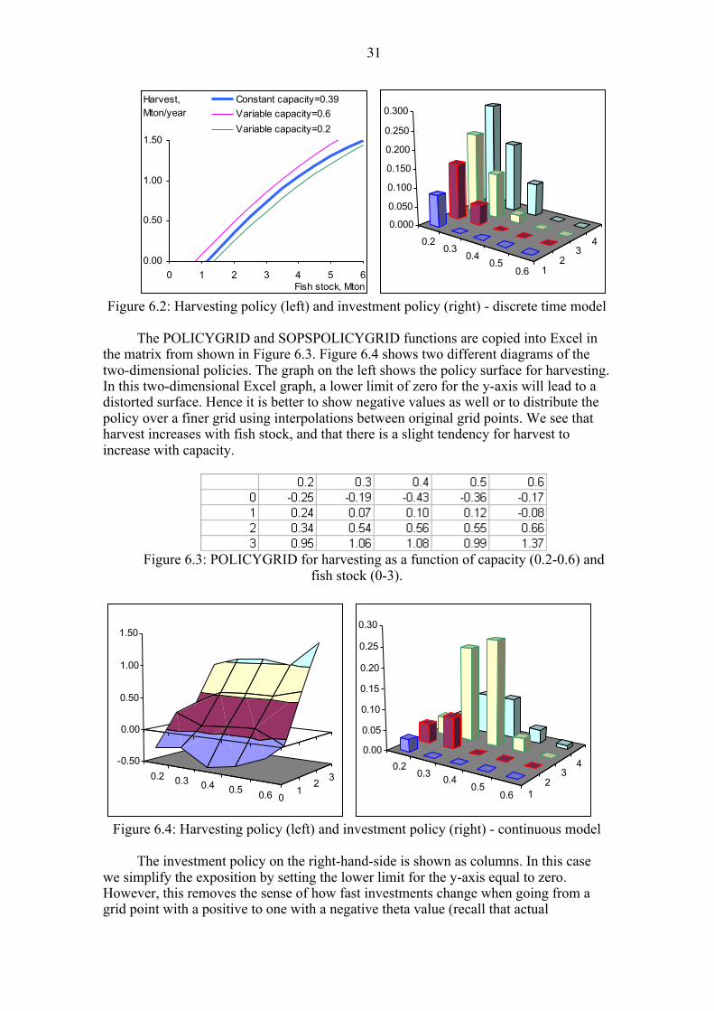
Figure 6.2 shows results from the discrete time model with two-dimensional

policies. The harvest policy from Figure 6.1 is repeated in the middle. The thin lines show how harvest changes when capacity is respectively increased to 0.6 or reduced to 0.2 Mton/year. Harvest increases with capacity. The linear investment policy shows that investments decrease with capacity (0.2 to 0.6 Mton/year) and increases with fish stock (1 to 4 Mton).

31

Harvest,Mton/year

0.00

0.50

1.00

1.50

0 1 2 3 4 5 6

Constant capacity=0.39Variable capacity=0.6Variable capacity=0.2

Fish stock, Mton

0.20.3

0.40.5

0.6 12

34

0.000

0.050

0.100

0.150

0.200

0.250

0.300

Figure 6.2: Harvesting policy (left) and investment policy (right) - discrete time model

The POLICYGRID and SOPSPOLICYGRID functions are copied into Excel in

the matrix from shown in Figure 6.3. Figure 6.4 shows two different diagrams of the two-dimensional policies. The graph on the left shows the policy surface for harvesting. In this two-dimensional Excel graph, a lower limit of zero for the y-axis will lead to a distorted surface. Hence it is better to show negative values as well or to distribute the policy over a finer grid using interpolations between original grid points. We see that harvest increases with fish stock, and that there is a slight tendency for harvest to increase with capacity.

Figure 6.3: POLICYGRID for harvesting as a function of capacity (0.2-0.6) and

fish stock (0-3).

0.2 0.3 0.4 0.5 0.6 01

2 3-0.50

0.00

0.50

1.00

1.50

0.20.3 0.4

0.50.6 1

23

40.00

0.05

0.10

0.15

0.20

0.25

0.30

Figure 6.4: Harvesting policy (left) and investment policy (right) - continuous model

The investment policy on the right-hand-side is shown as columns. In this case

we simplify the exposition by setting the lower limit for the y-axis equal to zero. However, this removes the sense of how fast investments change when going from a grid point with a positive to one with a negative theta value (recall that actual

32

investments are found by interpolation between grid points and extrapolations beyond grid points). We see a certain tendency for investments to increase with the fish stock and to decrease with capacity. But how important is this tendency?

0.2 0.30.4

0.50.6 0

12

3

0

20

40

60

80

100

0.20.3

0.40.5

0.6 12

34

010

20

30

40

50

60

70

Figure 6.5: Grid point importance, harvesting (left) and investment (right), 9 searches

Figure 6.5 shows results of the importance test described at the end of Section

5.2. Standard deviations are based on 9 selected policy searches; six more searches produced inferior solutions and were excluded. The standard deviation of initial policy parameters were respectively 0.5 and 0.2 for harvesting and investment policies.

For the harvesting policy we see that grid points for fish stocks in the range from

1 to 3 Mton and capacities in the range from 0.3 to 0.5 are most important. For the most important grid points, importance is close to 100 percent. We see that parameters for combined high capacity and low fish stocks are not important at all, consistent with what we saw in the upper right corner in Figure 5.11. Initial variation dominates in these cases and the theta values are neither reliable nor important. In practical use it seems better to set these values by intuition rather than to rely on the obtained parameter values. Another option is to narrow down the grid and repeat the optimization.

The investment policy has hardly any grid point of great importance; the highest

importance indicator is 69 percent. This is consistent with the finding that there is practically nothing to gain by allowing for variable capacity. However, when using a grid policy, the most reliable parameters are still important in keeping capacity close to its optimal level.

Finally, Excel or special purpose statistical packages could be used to estimate

analytical functions that capture the essence of policy surfaces resulting from grid functions. Such analytical functions could be useful for pedagogical purposes and may produce ideas for those that seek analytical solutions to complex stochastic problems.

33

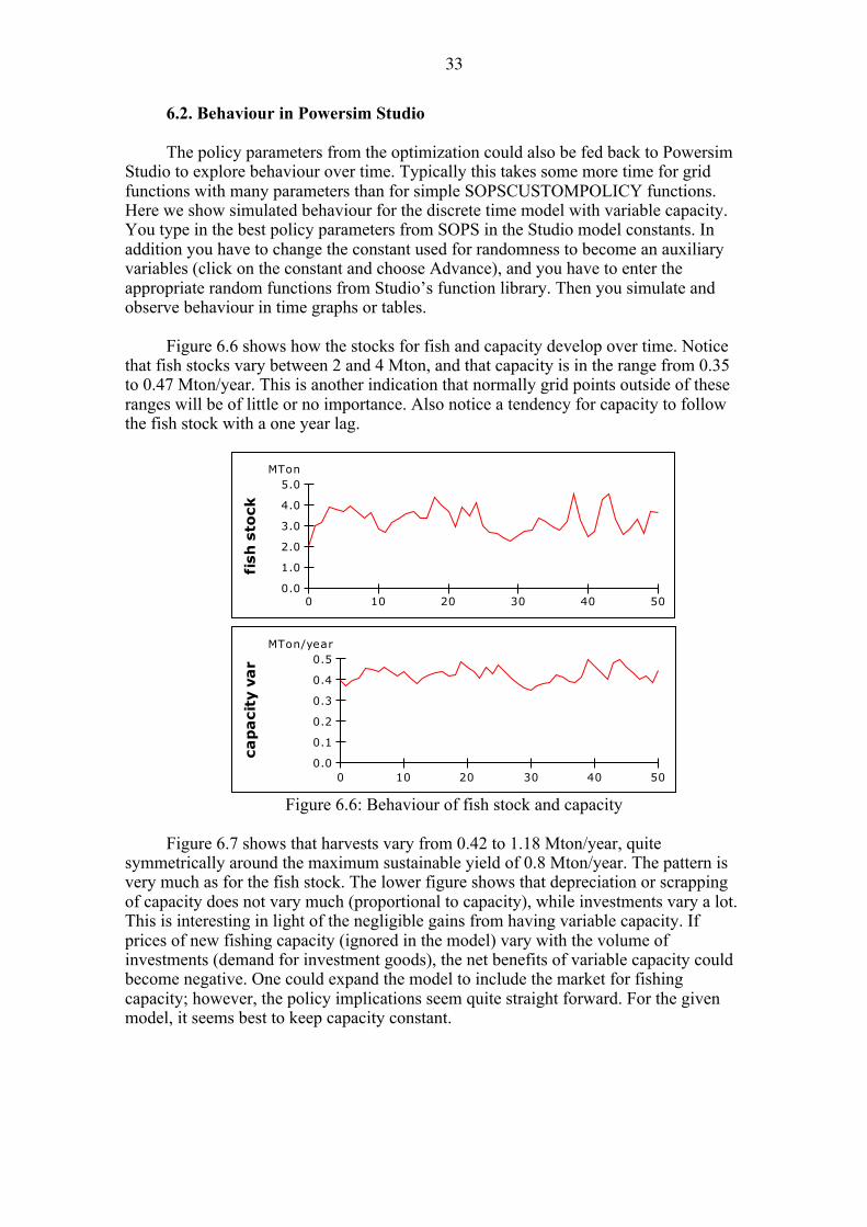
6.2. Behaviour in Powersim Studio The policy parameters from the optimization could also be fed back to Powersim

Studio to explore behaviour over time. Typically this takes some more time for grid functions with many parameters than for simple SOPSCUSTOMPOLICY functions. Here we show simulated behaviour for the discrete time model with variable capacity. You type in the best policy parameters from SOPS in the Studio model constants. In addition you have to change the constant used for randomness to become an auxiliary variables (click on the constant and choose Advance), and you have to enter the appropriate random functions from Studio’s function library. Then you simulate and observe behaviour in time graphs or tables.

Figure 6.6 shows how the stocks for fish and capacity develop over time. Notice

that fish stocks vary between 2 and 4 Mton, and that capacity is in the range from 0.35 to 0.47 Mton/year. This is another indication that normally grid points outside of these ranges will be of little or no importance. Also notice a tendency for capacity to follow the fish stock with a one year lag.

0 10 20 30 40 500.0

1.0

2.0

3.0

4.0

5.0MTon

fish

sto

ck

0 10 20 30 40 500.0

0.1

0.2

0.3

0.4

0.5MTon/year

cap

aci

ty v

ar

Figure 6.6: Behaviour of fish stock and capacity

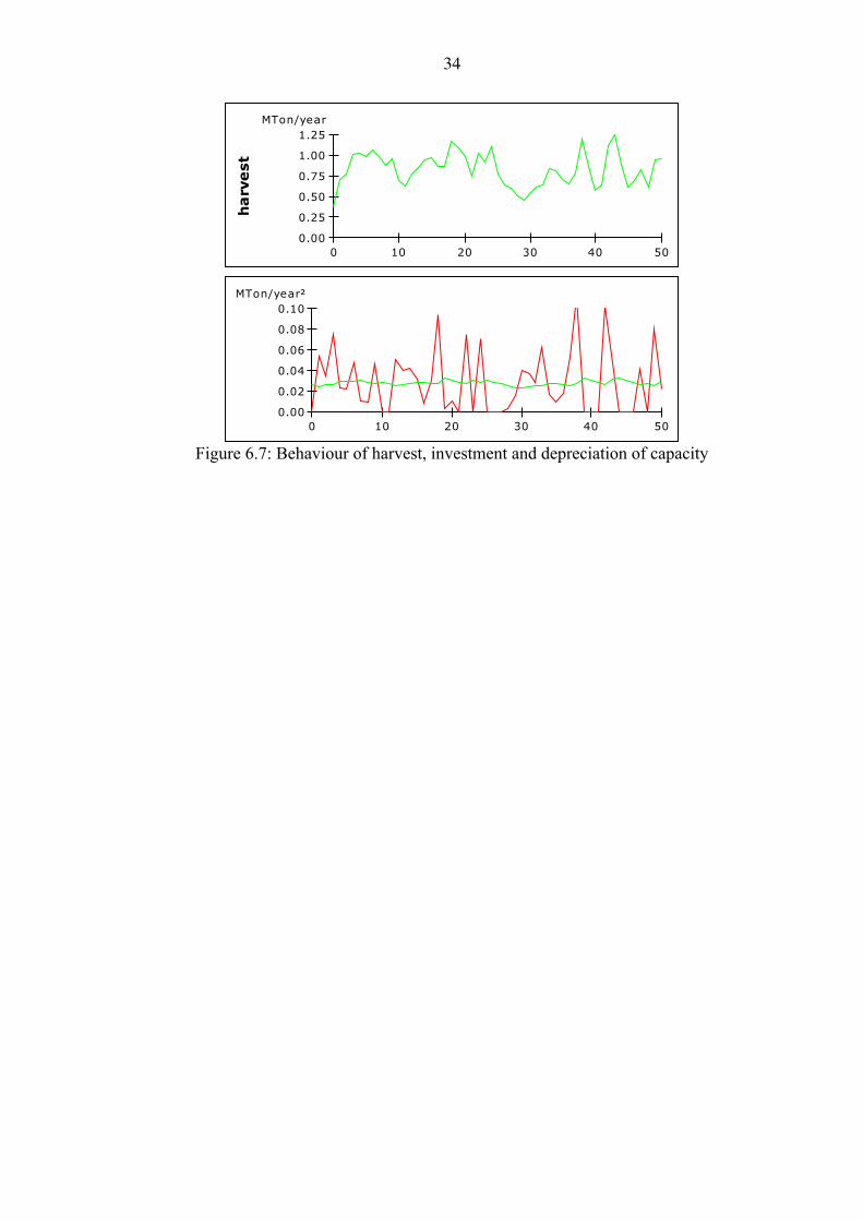
Figure 6.7 shows that harvests vary from 0.42 to 1.18 Mton/year, quite

symmetrically around the maximum sustainable yield of 0.8 Mton/year. The pattern is very much as for the fish stock. The lower figure shows that depreciation or scrapping of capacity does not vary much (proportional to capacity), while investments vary a lot. This is interesting in light of the negligible gains from having variable capacity. If prices of new fishing capacity (ignored in the model) vary with the volume of investments (demand for investment goods), the net benefits of variable capacity could become negative. One could expand the model to include the market for fishing capacity; however, the policy implications seem quite straight forward. For the given model, it seems best to keep capacity constant.

34

0 10 20 30 40 500.00

0.25

0.50

0.75

1.00

1.25MTon/year

harvest

0 10 20 30 40 500.00

0.02

0.04

0.06

0.08

0.10MTon/year²

Figure 6.7: Behaviour of harvest, investment and depreciation of capacity

35

APPENDIX 1: INSTALLING PROGRAMS

This appendix tells you how to install all needed programs.

A1.1. Powersim Studio

Powersim Studio can be bought and downloaded from the home page of Powersim Software: http://powersim.com/. The standard licence must be extended to use SOPS. However, for testing purposes you may download recent demo versions of Powersim Studio. These demo versions are time limited, but fully capable of running SOPS. You cannot use Studio Executive and Studio Player.

A1.2. SOPS with .Net and C++

Before you install SOPS (step 3) you must install the following two programs: Microsoft .Net and Microsoft C++ compiler. You probably have .Net already. If you do not have .Net, this package must be installed before you install C++ in step 2.

1. Install Microsoft .Net Framework 4 (free). Search for this software on internet.

These links have worked: http://www.microsoft.com/downloads/en/details.aspx?FamilyID=9cfb2d51-5ff4-

4491-b0e5-b386f32c0992 or http://www.microsoft.com/net

2. Install Microsoft’s Visual C++ 2010 Express (free) (SOPS should work also with newer releases than 2010). Search for this software on internet. This link has worked:

http://www.microsoft.com/visualstudio/en-us/products/2010-editions/visual-cpp-express

3. Install SOPS (free). This program enables you to perform optimization on your own Powersim Studio models, it also enables you to perform optimization on SOPS versions of Powersim Studio models that others have developed (.csim and .sops files). In the latter case you do not need a Powersim Studio licence to perform optimization, SOPS works as a Player version. The SOPS program can be installed from:

http://powersim.com You are now ready to use SOPS.

A1.3. Example models

The example models can be downloaded from: http://www.uib.no/rg/dynamics/research/software. You can download both the original Studio models (.sip) and the compiled SOPS

versions (.csim) with assumptions and results (.sops). This web page also contains this User’s manual.

36

APPENDIX 2: EXAMPLE MODEL EQUATIONS

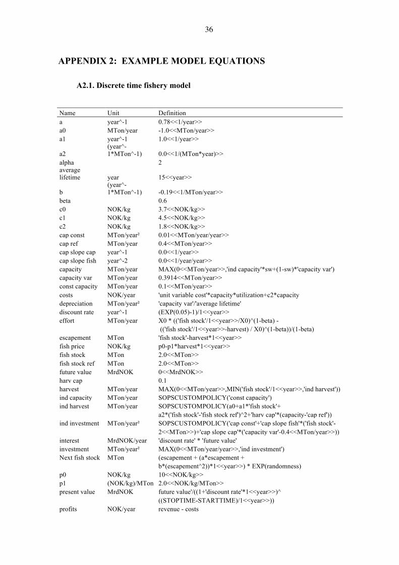
A2.1. Discrete time fishery model Name Unit Definition a year^-1 0.78<<1/year>> a0 MTon/year -1.0<<MTon/year>> a1 year^-1 1.0<<1/year>>

a2 (year^-1*MTon^-1) 0.0<<1/(MTon*year)>>

alpha 2 average lifetime year 15<<year>>

b (year^-1*MTon^-1) -0.19<<1/MTon/year>>

beta 0.6 c0 NOK/kg 3.7<<NOK/kg>> c1 NOK/kg 4.5<<NOK/kg>> c2 NOK/kg 1.8<<NOK/kg>> cap const MTon/year² 0.01<<MTon/year/year>> cap ref MTon/year 0.4<<MTon/year>> cap slope cap year^-1 0.0<<1/year>> cap slope fish year^-2 0.0<<1/year/year>> capacity MTon/year MAX(0<<MTon/year>>,'ind capacity'*sw+(1-sw)*'capacity var') capacity var MTon/year 0.3914<<MTon/year>> const capacity MTon/year 0.1<<MTon/year>> costs NOK/year 'unit variable cost'*capacity*utilization+c2*capacity depreciation MTon/year² 'capacity var'/'average lifetime' discount rate year^-1 (EXP(0.05)-1)/1<<year>> effort MTon/year X0 * (('fish stock'/1<<year>>/X0)^(1-beta) - (('fish stock'/1<<year>>-harvest) / X0)^(1-beta))/(1-beta) escapement MTon 'fish stock'-harvest*1<<year>> fish price NOK/kg p0-p1*harvest*1<<year>> fish stock MTon 2.0<<MTon>> fish stock ref MTon 2.0<<MTon>> future value MrdNOK 0<<MrdNOK>> harv cap 0.1 harvest MTon/year MAX(0<<MTon/year>>,MIN('fish stock'/1<<year>>,'ind harvest')) ind capacity MTon/year SOPSCUSTOMPOLICY('const capacity') ind harvest MTon/year SOPSCUSTOMPOLICY(a0+a1*'fish stock'+ a2*('fish stock'-'fish stock ref')^2+'harv cap'*(capacity-'cap ref')) ind investment MTon/year² SOPSCUSTOMPOLICY('cap const'+'cap slope fish'*('fish stock'- 2<<MTon>>)+'cap slope cap'*('capacity var'-0.4<<MTon/year>>)) interest MrdNOK/year 'discount rate' * 'future value' investment MTon/year² MAX(0<<MTon/year/year>>,'ind investment') Next fish stock MTon (escapement + (a*escapement + b*(escapement^2))*1<<year>>) * EXP(randomness) p0 NOK/kg 10<<NOK/kg>> p1 (NOK/kg)/MTon 2.0<<NOK/kg/MTon>> present value MrdNOK future value'/((1+'discount rate'*1<<year>>)^ ((STOPTIME-STARTTIME)/1<<year>>)) profits NOK/year revenue - costs

37

randomness 0 revenue NOK/year 'fish price'*harvest sw 1 unit variable cost NOK/kg c0+(c1-c0)*(utilization^alpha) update MTon/year ('Next fish stock'-'fish stock')/1<<year>> utilization effort/capacity X0 MTon/year 1.0<<MTon/year>>

38

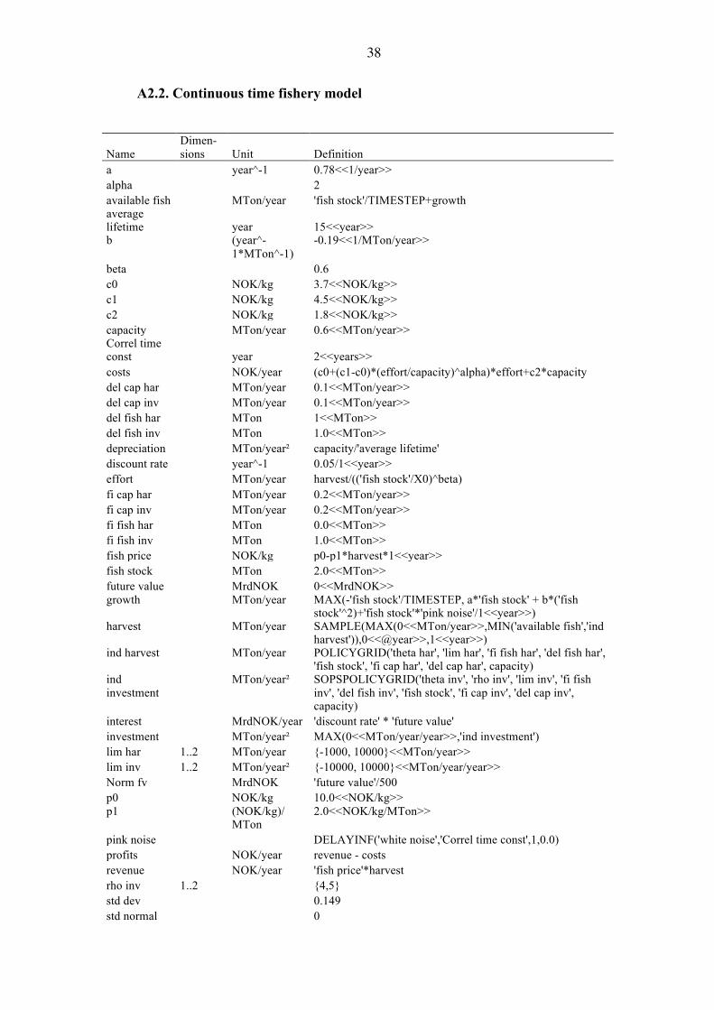
A2.2. Continuous time fishery model

Name Dimen-sions Unit Definition

a year^-1 0.78<<1/year>> alpha 2 available fish MTon/year 'fish stock'/TIMESTEP+growth average lifetime year 15<<year>> b

(year^-1*MTon^-1)

-0.19<<1/MTon/year>>

beta 0.6 c0 NOK/kg 3.7<<NOK/kg>> c1 NOK/kg 4.5<<NOK/kg>> c2 NOK/kg 1.8<<NOK/kg>> capacity MTon/year 0.6<<MTon/year>> Correl time const year 2<<years>> costs NOK/year (c0+(c1-c0)*(effort/capacity)^alpha)*effort+c2*capacity del cap har MTon/year 0.1<<MTon/year>> del cap inv MTon/year 0.1<<MTon/year>> del fish har MTon 1<<MTon>> del fish inv MTon 1.0<<MTon>> depreciation MTon/year² capacity/'average lifetime' discount rate year^-1 0.05/1<<year>> effort MTon/year harvest/(('fish stock'/X0)^beta) fi cap har MTon/year 0.2<<MTon/year>> fi cap inv MTon/year 0.2<<MTon/year>> fi fish har MTon 0.0<<MTon>> fi fish inv MTon 1.0<<MTon>> fish price NOK/kg p0-p1*harvest*1<<year>> fish stock MTon 2.0<<MTon>> future value MrdNOK 0<<MrdNOK>> growth

MTon/year

MAX(-'fish stock'/TIMESTEP, a*'fish stock' + b*('fish stock'^2)+'fish stock'*'pink noise'/1<<year>>)

harvest

MTon/year

SAMPLE(MAX(0<<MTon/year>>,MIN('available fish','ind harvest')),0<<@year>>,1<<year>>)

ind harvest

MTon/year

POLICYGRID('theta har', 'lim har', 'fi fish har', 'del fish har', 'fish stock', 'fi cap har', 'del cap har', capacity)

ind investment

MTon/year²

SOPSPOLICYGRID('theta inv', 'rho inv', 'lim inv', 'fi fish inv', 'del fish inv', 'fish stock', 'fi cap inv', 'del cap inv', capacity)

interest MrdNOK/year 'discount rate' * 'future value' investment MTon/year² MAX(0<<MTon/year/year>>,'ind investment') lim har 1..2 MTon/year {-1000, 10000}<<MTon/year>> lim inv 1..2 MTon/year² {-10000, 10000}<<MTon/year/year>> Norm fv MrdNOK 'future value'/500 p0 NOK/kg 10.0<<NOK/kg>> p1

(NOK/kg)/ MTon

2.0<<NOK/kg/MTon>>

pink noise DELAYINF('white noise','Correl time const',1,0.0) profits NOK/year revenue - costs revenue NOK/year 'fish price'*harvest rho inv 1..2 {4,5} std dev 0.149 std normal 0

39

theta har

1..4,1..5

MTon/year

{{0, 0, 0.0, 0.0, 0.0},{0.3, 0.3, 0.3, 0.3, 0.3},{0.5, 0.5, 0.5, 0.5, 0.5},{0.9, 0.9, 0.9, 0.9, 0.9}}<<MTon/year>>

theta inv

1..20

MTon/year²

{0.0, 0.0, 0.0, 0.0, 0.0, 0.03, 0.03, 0.03, 0.03, 0.03, 0.06, 0.06, 0.06, 0.06, 0.06, 0.10, 0.10, 0.10, 0.10, 0.10}<<MTon/year/year>>

white noise

0+'std dev'*SQRT(2.0*'Correl time const'/TIMESTEP-1)*'std normal'

X0 MTon 1.0<<MTon>>