Some properties and results involving the zeta and...
45
Functional Analysis, Approximation and Computation 7 (2) (2015), 89–133 Published by Faculty of Sciences and Mathematics, University of Niˇ s, Serbia Available at: http://www.pmf.ni.ac.rs/faac Some properties and results involving the zeta and associated functions H. M. Srivastava a a Department of Mathematics and Statistics, University of Victoria, Victoria, British Columbia V8W 3R4, Canada Abstract. In this research-cum-expository article, we aim at presenting a systematic account of some recent developments involving the Riemann Zeta function ζ (s), the Hurwitz (or general- ized) Zeta function ζ (s, a), and the Hurwitz-Lerch Zeta function Φ(z, s, a) as well as its various interesting extensions and generalizations. In particular, we begin by looking into the problems associated with the evaluations and representations of ζ (s) when s ∈ N \{1}, N being the set of natural numbers, emphasizing upon various potentially useful and computationally friendly classes of rapidly convergent series representations for ζ (2n + 1) (n ∈ N) which have been devel- oped in recent years. We then turn toward some other investigations involving certain general classes of Goldbach-Euler type sums. Finally, we present a systematic investigation of various properties and results involving several families of generating functions and their partial sums which are associated with the aforementioned general classes of the extended Hurwitz-Lerch Zeta functions. References to some of latest developments in the theory and applications of sev- eral families of the extended Hurwitz-Lerch zeta functions are also provided for the interested researchers on these and other related topics in Analytic Number Theory, Geometric Function Theory of Complex Analysis, and so on. 1. Introduction, Definitions and Preliminaries Throughout this article, we use the following standard notations: N := {1, 2, 3, ···}, N 0 := {0, 1, 2, 3, ···} = N ∪{0} and Z − := {−1, −2, −3, ···} = Z − 0 \{0}. 2010 Mathematics Subject Classification. Primary 11M06, 11M35, 33B15; Secondary 11B68, 33E20, 33E30. Keywords. Riemann Zeta function; Hurwitz (or generalized) Zeta function; Hurwitz-Lerch Zeta function; Asso- ciated Series and Integrals; Analytic Number Theory; Series representations; Harmonic numbers; Bernoulli numbers and Bernoulli polynomials; Generating functions; Euler numbers and Euler polynomials; Inductive argument; Sym- bolic and numerical computations; Dirichlet L-functions; Gamma and Psi (or Digamma) functions; Generalized Goldbach-Euler sums; Geometric Function Theory of Complex Analysis; Probability Distribution Theory. Received: 6 December 2014; Accepted: 12 January 2015 Communicated by Dragan S. Djordjevi´ c Email address: [email protected] (H. M. Srivastava)
Transcript of Some properties and results involving the zeta and...

Functional Analysis,Approximation andComputation7 (2) (2015), 89–133
Published by Faculty of Sciences and Mathematics,University of Nis, SerbiaAvailable at: http://www.pmf.ni.ac.rs/faac
Some properties and results involving the zetaand associated functions
H. M. Srivastavaa
aDepartment of Mathematics and Statistics, University of Victoria, Victoria, British Columbia V8W 3R4,Canada
Abstract. In this research-cum-expository article, we aim at presenting a systematic accountof some recent developments involving the Riemann Zeta function ζ(s), the Hurwitz (or general-ized) Zeta function ζ(s, a), and the Hurwitz-Lerch Zeta function Φ(z, s, a) as well as its variousinteresting extensions and generalizations. In particular, we begin by looking into the problemsassociated with the evaluations and representations of ζ (s) when s ∈ N \ 1, N being the setof natural numbers, emphasizing upon various potentially useful and computationally friendlyclasses of rapidly convergent series representations for ζ (2n+ 1) (n ∈ N) which have been devel-oped in recent years. We then turn toward some other investigations involving certain generalclasses of Goldbach-Euler type sums. Finally, we present a systematic investigation of variousproperties and results involving several families of generating functions and their partial sumswhich are associated with the aforementioned general classes of the extended Hurwitz-LerchZeta functions. References to some of latest developments in the theory and applications of sev-eral families of the extended Hurwitz-Lerch zeta functions are also provided for the interestedresearchers on these and other related topics in Analytic Number Theory, Geometric FunctionTheory of Complex Analysis, and so on.
1. Introduction, Definitions and Preliminaries
Throughout this article, we use the following standard notations:
N := 1, 2, 3, · · · , N0 := 0, 1, 2, 3, · · · = N ∪ 0
andZ− := −1,−2,−3, · · · = Z−
0 \ 0.
2010 Mathematics Subject Classification. Primary 11M06, 11M35, 33B15; Secondary 11B68, 33E20, 33E30.Keywords. Riemann Zeta function; Hurwitz (or generalized) Zeta function; Hurwitz-Lerch Zeta function; Asso-
ciated Series and Integrals; Analytic Number Theory; Series representations; Harmonic numbers; Bernoulli numbersand Bernoulli polynomials; Generating functions; Euler numbers and Euler polynomials; Inductive argument; Sym-bolic and numerical computations; Dirichlet L-functions; Gamma and Psi (or Digamma) functions; GeneralizedGoldbach-Euler sums; Geometric Function Theory of Complex Analysis; Probability Distribution Theory.
Received: 6 December 2014; Accepted: 12 January 2015Communicated by Dragan S. DjordjevicEmail address: [email protected] (H. M. Srivastava)

H. M. Srivastava / FAAC 7 (2) (2015), 89–133 90
Also, as usual, Z denotes the set of integers, R denotes the set of real numbers, R+ denotes theset of positive numbers and C denotes the set of complex numbers.
Some rather important and potentially useful functions in Analytic Number Theory include (forexample) the Riemann Zeta function ζ(s) and the Hurwitz (or generalized) Zeta function ζ(s, a),which are defined (for ℜ (s) > 1) by
ζ (s) :=
∞∑n=1
1
ns=
1
1− 2−s
∞∑n=1
1
(2n− 1)s
(ℜ (s) > 1
)1
1− 21−s
∞∑n=1
(−1)n−1
ns(ℜ (s) > 0; s = 1
) (1.1)
and
ζ (s, a) :=
∞∑k=0
1
(k + a)s
(ℜ (s) > 1; a ∈ C \ Z−
0
)= ζ(s, n+ a) +
n−1∑k=0
1
(k + a)s(n ∈ N), (1.2)
and(for ℜ (s) 5 1; s = 1
)by their meromorphic continuations (see, for details, the excellent
works by Titchmarsh [104] and Apostol [6] as well as the monumental treatise by Whittaker andWatson [107]; see also [1, Chapter 23] and [83, Chapter 2]), so that (obviously)
ζ (s, 1) = ζ (s) = (2s − 1)−1
ζ
(s,
1
2
)and ζ (s, 2) = ζ (s)− 1. (1.3)
Indeed, in many different ways, both of the Zeta functions ζ(s) and ζ(s, a) can be continuedmeromorphically to the whole complex s-plane except for a simple pole at s = 1 with their respectiveresidues 1.
The following simple relationships between the Zeta functions ζ(s) and ζ(s, a) are worthy ofnote:
ζ (s) =1
ms − 1
m−1∑j=1
ζ
(s,j
m
)(m ∈ N \ 1) (1.4)
and
ζ (s,ma) =1
ms
m−1∑j=0
ζ
(s, a+
j
m
)(m ∈ N) . (1.5)
A classical about three-century-old theorem of Christian Goldbach (1690–1764) was stated ina letter dated 1729 from Goldbach to Daniel Bernoulli (1700–1782). Goldbach’s Theorem wasrevived and revisited recently in many publications as the following problem:
∑ω∈S
1
ω − 1= 1, (1.6)
where S denotes the set of all nontrivial integer kth powers, that is,
S :=nk : n, k ∈ N \ 1 = 2, 3, 4, · · ·
.

H. M. Srivastava / FAAC 7 (2) (2015), 89–133 91
In fact, in terms of the Riemann Zeta function ζ(s) defined by (1.1), Goldbach’s theorem (1.6) caneasily be seen to assume the following elegant form:
∑ω∈S
1
ω − 1=
∞∑k=2
[ζ(k)− 1] = 1. (1.7)
Since ζ(s) is a decreasing function of its argument s for s = 2, we have
1 < ζ(n) 5 ζ(2) =π2
6< 2, (1.8)
the above alternative form (1.7) of Goldbach’s Theorem (1.6) can also be rewritten as follows:
∞∑k=2
f(ζ(k)
)= 1,
where
f(x) := x− [x] = The fractional part of x ∈ R.
As a matter of fact, it is fairly straightforward to show also that
∞∑k=2
(−1)k f(ζ(k)
)=
1
2,
∞∑k=1
f(ζ(2k)
)=
3
4and
∞∑k=1
f(ζ(2k + 1)
)=
1
4.
It may be of interest to remark in passing that the name of Christian Goldbach (1690–1764)is usually associated with a relatively more popular conjecture dated 1742 (known as Goldbach’sConjecture) that every positive integer greater than 2 is the sum of two prime numbers:
4 = 2 + 2 = 1 + 3; 6 = 3 + 3 = 1 + 5; 8 = 1 + 7 = 3 + 5; et cetera.
Just as the celebrated Riemann Hypothesis dated 1859 that all nontrivial zeros of ζ(s) lie onthe critical line:
ℜ(s) = 1
2,
Goldbach’s conjecture has not been proven as yet. Interestingly, not too long ago in the year 2001,on the occasion of the publication of the following (“very funny, tender, charming, and irresistible”)novel:
Uncle Pedros and Goldbach’s Conjecture: A Novel of Mathematical Obsession (byApostolos Doxiadis), Faber and Faber, London, 2001,
the British publisher (Faber and Faber) had offered a reward of one million U.K. Pounds to anyonewho can prove Goldbach’s Conjecture.
Another result that has attracted fascinatingly and tantalizingly large number of seeminglyindependent solutions is the so-called Basler Problem:
ζ(2) =π2
6, (1.9)
H. M. Srivastava / FAAC 7 (2) (2015), 89–133 92
which was used above in (1.8). It was of vital importance to Leonhard Euler (1707-1783) andthe Bernoulli brothers [Jakob Bernoulli (1654-1705) and Johann Bernoulli (1667-1748)]. All theseremarkably many essentially independent solutions of the Basler Problem (1.9) have appearedin the mathematical literature ever since Euler first solved this problem in the year 1736. Inthis context, one other remarkable classical result involving Riemann’s Zeta function ζ(s) is thefollowing elegant series representation for ζ (3):
ζ (3) = −4π2
7
∞∑k=0
ζ (2k)
(2k + 1) (2k + 2) · 22k, (1.10)
which was actually contained in Euler’s 1772 paper entitled “Exercitationes Analyticae” (cf., e.g.,Ayoub [7, pp. 1084–1085]). Remarkably, this 1772 result (1.10) of Euler was rediscovered (amongothers) by Ramaswami [64] (see also a paper by Srivastava [71, p. 7, Equation (2.23)]) and (morerecently) by Ewell [26]. Moreover, just as pointed out by (for example) Chen and Srivastava [14,pp. 180–181], another series representation:
ζ (3) =5
2
∞∑k=1
(−1)k−1
k3(2k
k
) , (1.11)
which played a key role in the celebrated proof (see, for details, [5]) of the irrationality of ζ (3)by Roger Apery (1916-1994), was derived independently by (among others) Hjortnaes [40], Gosper[34], and Apery [5] himself.
It is easily observed that Euler’s series in (1.10) converges faster than the defining series forζ (3), but obviously not as fast as the series in (1.11). Evaluations of such Zeta values as ζ (3),ζ (5), et cetera are known to arise naturally in a wide variety of applications such as those inElastostatics, Quantum Field Theory, et cetera (see, for example, Tricomi [105], Witten [109], andNash and O’Connor [57], [58]). On the other hand, in the case of even integer arguments, wealready have the following computationally useful relationship:
ζ (2n) = (−1)n−1 (2π)
2n
2 · (2n)!B2n (n ∈ N0) (1.12)
with the well-tabulated Bernoulli numbers defined by the following generating function:
z
ez − 1=
∞∑n=0
Bnzn
n!(|z| < 2π) , (1.13)
as well as the following familiar recursion formula:
ζ (2n) =
(n+
1
2
)−1 n−1∑k=1
ζ (2k) ζ (2n− 2k) (n ∈ N \ 1) , (1.14)
which, in terms of the Bernoulli numbers Bn, can be rewritten at once as follows:
B2n = − 1
2n+ 1
n−1∑k=1
(2n
2k
)B2kB2n−2k (n ∈ N \ 1) . (1.15)
This research-cum-expository article is motivated largely by several recent works by Srivastavaet al. (see, for example, [19], [80] and [81]). It consists of four major parts. In the first part, agenuine need (for computational purposes) for expressing ζ (2n+ 1) as a rapidly converging series
H. M. Srivastava / FAAC 7 (2) (2015), 89–133 93
for all n ∈ N has been shown to lead naturally to a rather systematic investigation of the variousinteresting families of rapidly convergent series representations for the Riemann ζ (2n+ 1) (n ∈ N).Relevant connections of the results presented here with many other known series representationsfor ζ (2n+ 1) (n ∈ N) are also briefly indicated. In fact, for two of the many computationallyuseful special cases considered here, it has been observed that ζ (3) can be represented by meansof series which converge much more rapidly than that in Euler’s celebrated formula (1.10) aswell as that in the series (1.11) which (just as we indicated above) was used earlier by Apery [5]in his celebrated proof of the irrationality of ζ (3). Symbolic and numerical computations usingMathematica (Version 4.0) for Linux have shown, among other things, that only 50 terms of oneof these series are capable of producing an accuracy of seven decimal places. In the second partof this article, we consider a variety of series and integrals associated with the Hurwitz-Lerch Zetafunction Φ(z, s, a) as well as its various interesting extensions and generalizations (see Section 6).In our next two sections (Section 7 and Section 8), we present a systematic account of some recentdevelopments involving certain general classes of Goldbach-Euler type sums as well as variousproperties and results involving several families of generating functions and their partial sumswhich are associated with the aforementioned general classes of the extended Hurwitz-Lerch Zetafunctions which we introduced in Section 6. Finally, in our last section (Section 9), we choose topresent several further closely-related remarks and observations about the developments consideredin Section 6 and Section 8 in addition (for example) to the Open Problem mentioned in Section 7.
2. Rapidly Converging Series for ζ (2n + 1) (n ∈ N)
Suppose, as usual, that (λ)ν denotes the Pochhammer symbol or the shifted factorial, since
(1)n = n! (n ∈ N0),
which is defined, in terms of the familiar Gamma function, by
(λ)ν :=Γ(λ+ ν)
Γ(λ)=
1 (ν = 0; λ ∈ C \ 0)
λ(λ+ 1) · · · (λ+ n− 1) (ν = n ∈ N; λ ∈ C),
it being understood conventionally that (0)0 := 1 and assumed tacitly that the Γ-quotient exists(see, for details, [72] and [83]). In terms of the above-defined Pochhammer symbol (λ)ν , we beginthis section by recalling the following simple consequence of the binomial theorem and the definition(1.1):
∞∑k=0
(s)kk!
ζ (s+ k, a) tk = ζ (s, a− t) (|t| < |a|) , (2.1)
which, for a = 1 and t = ±1/m, yields a useful series identity given by
∞∑k=0
(s)2k(2k)!
ζ (s+ 2k)
m2k
=
(2s − 1) ζ (s)− 2s−1 (m = 2)
1
2
[(ms − 1) ζ (s)−ms −
m−2∑j=2
ζ
(s,j
m
)](m ∈ N \ 1, 2) .
(2.2)

H. M. Srivastava / FAAC 7 (2) (2015), 89–133 94
By making use of the familiar harmonic numbers Hn given by
Hn :=
n∑j=1
1
j(n ∈ N) , (2.3)
the following set of series representations for ζ (2n+ 1) (n ∈ N) were proven by Srivastava [75] byappealing appropriately to the series identity (2.2) in its special cases when m = 2, 3, 4, and 6,and also to many other properties and characteristics of the Riemann Zeta function such as thefamiliar functional equation:
ζ (s) = 2 · (2π)s−1sin
(1
2πs
)Γ (1− s) ζ (1− s) (2.4)
or, equivalently,
ζ (1− s) = 2 · (2π)−scos
(1
2πs
)Γ (s) ζ (s) , (2.5)
the familiar derivative formula:
ζ ′ (−2n) = limε→0
ζ (−2n+ ε)
ε
=
(−1)n
2 · (2π)2n(2n)! ζ (2n+ 1) (n ∈ N) (2.6)
with, of course,
ζ (0) = −1
2; ζ (−2n) = 0 (n ∈ N) ; ζ ′ (0) = −1
2log (2π) , (2.7)
and each of the following limit relationships:
lims→−2n
sin(12πs
)s+ 2n
= (−1)
n π
2(n ∈ N) (2.8)
and
lims→−2n
ζ (s+ 2k)
s+ 2n
=
(−1)n−k
2 · (2π)2(n−k)(2n− 2k)! ζ (2n− 2k + 1)
(k = 1, . . . , n− 1; n ∈ N \ 1) . (2.9)
Series Representation of the First Kind:
ζ (2n+ 1) = (−1)n−1 (2π)
2n
22n+1 − 1
[H2n − log π
(2n)!+
n−1∑k=1
(−1)k
(2n− 2k)!
ζ (2k + 1)
π2k
+2∞∑k=1
(2k − 1)!
(2n+ 2k)!
ζ (2k)
22k
](n ∈ N) . (2.10)
Series Representation of the Second Kind:
ζ (2n+ 1) = (−1)n−1 2 · (2π)2n
32n+1 − 1
[H2n − log
(23π)
(2n)!+
n−1∑k=1
(−1)k
(2n− 2k)!
ζ (2k + 1)(23π)2k
+2
∞∑k=1
(2k − 1)!
(2n+ 2k)!
ζ (2k)
32k
](n ∈ N) . (2.11)

H. M. Srivastava / FAAC 7 (2) (2015), 89–133 95
Series Representation of the Third Kind:
ζ (2n+ 1) = (−1)n−1 2 · (2π)2n
24n+1 + 22n − 1
[H2n − log
(12π)
(2n)!
+n−1∑k=1
(−1)k
(2n− 2k)!
ζ (2k + 1)(12π)2k + 2
∞∑k=1
(2k − 1)!
(2n+ 2k)!
ζ (2k)
42k
](n ∈ N) . (2.12)
Series Representation of the Fourth Kind:
ζ (2n+ 1) = (−1)n−1 2 · (2π)2n
32n (22n + 1) + 22n − 1
[H2n − log
(13π)
(2n)!
+n−1∑k=1
(−1)k
(2n− 2k)!
ζ (2k + 1)(13π)2k + 2
∞∑k=1
(2k − 1)!
(2n+ 2k)!
ζ (2k)
62k
](n ∈ N) . (2.13)
Here, as well as elsewhere in this presentation, an empty sum is understood (as usual) to be zero.The first series representation (2.10) is markedly different from each of the series representations
for ζ (2n+ 1), which were given earlier by Zhang and Williams [112, p. 1590, Equation (3.13)]and (subsequently) by Cvijovic and Klinowski [21, p. 1265, Theorem A] (see also [113] and [114]).Since ζ (2k) → 1 as k → ∞, the general term in the series representation (2.10) has the followingorder estimate:
O(2−2k · k−2n−1
)(k → ∞; n ∈ N) ,
whereas the general term in each of the aforecited earlier series representations has the orderestimate given below:
O(2−2k · k−2n
)(k → ∞; n ∈ N) .
By suitably combining (2.10) and (2.12), we easily arrive at the following series representation:
ζ (2n+ 1) = (−1)n−1 2 · (2π)2n
(22n − 1) (22n+1 − 1)
[log 2
(2n)!
+n−1∑k=1
(−1)k (
22k − 1)
(2n− 2k)!
ζ (2k + 1)
π2k
−2∞∑k=1
(2k − 1)!(22k − 1
)(2n+ 2k)!
ζ (2k)
24k
](n ∈ N) . (2.14)
Furthermore, in terms of the Bernoulli numbers Bn and the Euler polynomials En (x) defined bythe generating functions (1.9) and
2exz
ez + 1=
∞∑n=0
En (x)zn
n!(|z| < π) , (2.15)
respectively, it is known that (cf., e.g., [54, p. 29])
En (0) = (−1)nEn (1) =
2(1− 2n+1
)n+ 1
Bn+1 (n ∈ N) . (2.16)
Thus, by combining (2.16) with the identity (1.12), we find that
E2n−1 (0) =4 · (−1)
n
(2π)2n (2n− 1)!
(22n − 1
)ζ (2n) (n ∈ N) . (2.17)
H. M. Srivastava / FAAC 7 (2) (2015), 89–133 96
If we apply the relationship (2.17), the series representation (2.14) can immediately be put in thefollowing alternative form:
ζ (2n+ 1) = (−1)n−1 2 · (2π)2n
(22n − 1) (22n+1 − 1)
[log 2
(2n)!
+n−1∑k=1
(−1)k (
22k − 1)
(2n− 2k)!
ζ (2k + 1)
π2k
+1
2
∞∑k=1
(−1)k−1
(2n+ 2k)!
(π2
)2kE2k−1 (0)
](n ∈ N) , (2.18)
which is a slightly modified and corrected version of a result proven, using a significantly differenttechnique, by Tsumura [106, p. 383, Theorem B].
One other interesting combination of the series representations (2.10) and (2.12) leads us tothe following variant of Tsumura’s result (2.14) or (2.18):
ζ (2n+ 1) = (−1)n−1 π2n
22n+1 − 1
[H2n − log
(14π)
(2n)!
+
n−1∑k=1
(−1)k (
22k+1 − 1)
(2n− 2k)!
ζ (2k + 1)
π2k
−4∞∑k=1
(2k − 1)!(22k−1 − 1
)(2n+ 2k)!
ζ (2k)
24k
](n ∈ N) , (2.19)
which is essentially the same as the determinantal expression for ζ (2n+ 1) derived by Ewell [27,p. 1010, Corollary 3] by employing an entirely different technique from ours.
Numerous other similar combinations of the series representations (2.10) to (2.13) would yieldsome interesting companions of Ewell’s result (2.19).
Next, by setting t = 1/m and differentiating both sides with respect to s, we find from thefollowing obvious consequence of the series identity (2.1):
∞∑k=0
(s)2k+1
(2k + 1)!ζ (s+ 2k + 1, a) t2k+1
=1
2[ζ (s, a− t)− ζ (s, a+ t)] (|t| < |a|) (2.20)
that
∞∑k=0
(s)2k+1
(2k + 1)! m2k
ζ ′ (s+ 2k + 1, a) + ζ (s+ 2k + 1, a)2k∑j=0
1
s+ j
=m
2
∂
∂s
ζ
(s, a− 1
m
)− ζ
(s, a+
1
m
)(m ∈ N \ 1) . (2.21)
In the particular case when m = 2, (2.21) immediately yields
∞∑k=0
(s)2k+1
(2k + 1)! 22k
ζ ′ (s+ 2k + 1, a) + ζ (s+ 2k + 1, a)2k∑j=0
1
s+ j
= −
(a− 1
2
)−s
log
(a− 1
2
). (2.22)

H. M. Srivastava / FAAC 7 (2) (2015), 89–133 97
Upon letting s → −2n − 1 (n ∈ N) in the further special of this last identity (2.22) when a = 1,Wilton [83, p. 92] deduced the following series representation for ζ (2n+ 1) (see also [39, p. 357,Entry (54.6.9)]):
ζ (2n+ 1) = (−1)n−1
π2n
[H2n+1 − log π
(2n+ 1)!+
n−1∑k=1
(−1)k
(2n− 2k + 1)!
ζ (2k + 1)
π2k
+2∞∑k=1
(2k − 1)!
(2n+ 2k + 1)!
ζ (2k)
22k
](n ∈ N) , (2.23)
which, in light of the elementary identity:
(2k)!
(2n+ 2k)!=
(2k − 1)!
(2n+ 2k − 1)!− 2n
(2k − 1)!
(2n+ 2k)!(n ∈ N) , (2.24)
would combine with the result (2.10) to yield the following series representation:
ζ (2n+ 1) = (−1)n (2π)
2n
n (22n+1 − 1)
[n−1∑k=1
(−1)k−1
k
(2n− 2k)!
ζ (2k + 1)
π2k
+
∞∑k=0
(2k)!
(2n+ 2k)!
ζ (2k)
22k
](n ∈ N) . (2.25)
This last series representation (2.25) is precisely the aforementioned main result of Cvijovicand Klinowski [21, p. 1265, Theorem A]. As a matter of fact, in view of a known derivative formula[75, p. 389, Equation (2.8)], the series representation (2.25) is essentially the same as a result givenearlier by Zhang and Williams [112, p. 1590, Equation (3.13)] (see also Zhang and Williams [112,p. 1591, Equation (3.16)] where an obviously more complicated (asymptotic) version of (2.25) wasproven similarly).
By making use of another elementary identity:
(2k)!
(2n+ 2k + 1)!=
(2k − 1)!
(2n+ 2k)!− (2n+ 1)
(2k − 1)!
(2n+ 2k + 1)!(n, k ∈ N) , (2.26)
we can obtain the following yet another series representation for ζ (2n+ 1) by applying (2.10) and(2.23):
ζ (2n+ 1) = (−1)n 2 · (2π)2n
(2n− 1) 22n + 1
[n−1∑k=1
(−1)k−1
k
(2n− 2k + 1)!
ζ (2k + 1)
π2k
+∞∑k=0
(2k)!
(2n+ 2k + 1)!
ζ (2k)
22k
](n ∈ N) , (2.27)
which provides a significantly simpler (and much more rapidly convergent) version of the followingother main result of Cvijovic and Klinowski [21, p. 1265, Theorem B]:
ζ (2n+ 1) = (−1)n 2 · (2π)2n
(2n)!
∞∑k=0
Ωn,kζ (2k)
22k(n ∈ N) , (2.28)
where the coefficients Ωn,k (n ∈ N; k ∈ N0) are given explicitly as a finite sum of Bernoulli numbers[21, p. 1265, Theorem B(i)] (see, for details, Srivastava [75, pp. 393-394]):
Ωn,k :=2n∑j=0
(2n
j
)B2n−j
(j + 2k + 1) (j + 1) 2j(n ∈ N; k ∈ N0) . (2.29)
H. M. Srivastava / FAAC 7 (2) (2015), 89–133 98
3. Further Classes of Rapidly Convergent Series for ζ (2n + 1) (n ∈ N)
We begin this section once again from the identity (2.1) with (of course) a = 1, t = ±1/m, ands replaced by s+1. Thus, by applying (2.2), we find yet another class of series identities including,for example,
∞∑k=1
(s+ 1)2k(2k)!
ζ (s+ 2k)
22k= (2s − 2) ζ (s) (3.1)
and
∞∑k=1
(s+ 1)2k(2k)!
ζ (s+ 2k)
m2k
=1
2m
[m (ms − 3) ζ (s) +
(ms+1 − 1
)ζ (s+ 1)− 2ζ
(s+ 1,
1
m
)
−m−2∑j=2
mζ
(s,j
m
)+ ζ
(s+ 1,
j
m
) (m ∈ N \ 1, 2) . (3.2)
In fact, it is the series identity (3.1) which was first applied by Zhang and Williams [112] (and,subsequently, by Cvijovic and Klinowski [21]) with a view to proving two (only seemingly different)versions of the series representation (2.25). Indeed, if we appeal to (3.2) with m = 4, we can derivethe following much more rapidly convergent series representation for ζ (2n+ 1) (see [74, p. 9,Equation (41)]):
ζ (2n+ 1) = (−1)n 2 · (2π)2n
n (24n+1 + 22n − 1)
[4n−1 − 1
(2n)!B2n log 2
− 22n−1 − 1
2 (2n− 1)!ζ ′ (1− 2n)− 42n−1
(2n− 1)!ζ ′(1− 2n,
1
4
)+
n−1∑k=1
(−1)k−1
k
(2n− 2k)!
ζ (2k + 1)(12π)2k +
∞∑k=0
(2k)!
(2n+ 2k)!
ζ (2k)
42k
](n ∈ N) , (3.3)
where (and in what follows) a prime denotes the derivative of ζ (s) or ζ (s, a) with respect to s.
By means of the identities (2.24) and (2.26), the results (2.12) and (3.3) would lead us eventuallyto the following additional series representations for ζ (2n+ 1) (n ∈ N) (see [74, p. 10, Equations(42) and (43)]):
ζ (2n+ 1) = (−1)n−1
(π2
)2n [H2n+1 − log(12π)
(2n+ 1)!+
2 (4n − 1)
(2n+ 2)!B2n+2 log 2
− 22n+1 − 1
(2n+ 1)!ζ ′ (−2n− 1)− 24n+3
(2n+ 1)!ζ ′(−2n− 1,
1
4
)+
n−1∑k=1
(−1)k
(2n− 2k + 1)!
ζ (2k + 1)(12π)2k + 2
∞∑k=1
(2k − 1)!
(2n+ 2k + 1)!
ζ (2k)
42k
](n ∈ N)
(3.4)
H. M. Srivastava / FAAC 7 (2) (2015), 89–133 99
and
ζ (2n+ 1) = (−1)n 4 · (2π)2n
n · 42n+1 − 22n + 1
[22n+1 − 1
2 · (2n)!ζ ′ (−2n− 1)
+42n+1
(2n)!ζ ′(−2n− 1,
1
4
)− (2n+ 1) (4n − 1)
(2n+ 2)!B2n+2 log 2
+
n−1∑k=1
(−1)k−1
k
(2n− 2k + 1)!
ζ (2k + 1)(12π)2k +
∞∑k=0
(2k)!
(2n+ 2k + 1)!
ζ (2k)
42k
](n ∈ N) .
(3.5)
Explicit expressions for the derivatives ζ ′ (−2n± 1) and ζ ′(−2n± 1, 14
), which are involved in
the series representations (3.3), (3.4) and (3.5), can be found and substituted into these results inorder to represent ζ (2n+ 1) in terms of Bernoulli numbers and polynomials and various rapidlyconvergent series of the ζ-functions (see, for details, the work by Srivastava [74, Section 3]).
Out of the four seemingly analogous results (2.12), (3.3), (3.4) and (3.5), the infinite series in(3.4) would obviously converge most rapidly, with its general term having the order estimate:
O(k−2n−2 · 4−2k
)(k → ∞; n ∈ N) .
Now, from the work by Srivastava and Tsumura [100], we recall the following three new membersof the class of the series representations (2.12) and (3.4):
ζ (2n+ 1) = (−1)n−1
(2π
3
)2n[H2n+1 − log
(23π)
(2n+ 1)!+
(32n+2 − 1
)π
2√3 (2n+ 2)!
B2n+2
+(−1)
n−1
√3 (2π)
2n+1 ζ
(2n+ 2,
1
3
)
+n−1∑k=1
(−1)k
(2n− 2k + 1)!
ζ (2k + 1)(23π)2k + 2
∞∑k=1
(2k − 1)!
(2n+ 2k + 1)!
ζ (2k)
32k
](n ∈ N) ,
(3.6)
ζ (2n+ 1) = (−1)n−1
(π2
)2n [H2n+1 − log(12π)
(2n+ 1)!+
22n(22n+2 − 1
)π
(2n+ 2)!B2n+2
+(−1)
n−1
2 · (2π)2n+1 ζ
(2n+ 2,
1
4
)
+
n−1∑k=1
(−1)k
(2n− 2k + 1)!
ζ (2k + 1)(12π)2k + 2
∞∑k=1
(2k − 1)!
(2n+ 2k + 1)!
ζ (2k)
42k
](n ∈ N) ,
(3.7)
and
ζ (2n+ 1) = (−1)n−1
(π3
)2n [H2n+1 − log(13π)
(2n+ 1)!+
22n(32n+2 − 1
)π
√3 (2n+ 2)!
B2n+2
+(−1)
n−1
2√3 (2π)
2n+1
ζ
(2n+ 2,
1
3
)+ ζ
(2n+ 2,
1
6
)
+n−1∑k=1
(−1)k
(2n− 2k + 1)!
ζ (2k + 1)(13π)2k + 2
∞∑k=1
(2k − 1)!
(2n+ 2k + 1)!
ζ (2k)
62k
](n ∈ N) .
(3.8)
H. M. Srivastava / FAAC 7 (2) (2015), 89–133 100
The general terms of the infinite series occurring in these three members (3.6), (3.7) and (3.8) havethe following order estimates:
O(k−2n−2 ·m−2k
)(k → ∞; n ∈ N; m = 3, 4, 6) , (3.9)
which exhibit the fact that each of these last three series representations (3.6), (3.7), and (3.8)converges more rapidly than Wilton’s result (2.23) and two of them [cf. Equations (3.7) and (3.8)]at least as rapidly as Srivastava’s result (3.4).
We next recall that, in their aforementioned work on the Ray-Singer torsion and topological fieldtheories, Nash and O’Connor ([57] and [58]) obtained a number of remarkable integral expressionsfor ζ (3), including (for example) the following result [26, p. 1489 et seq.]:
ζ (3) =2π2
7log 2− 8
7
∫ π/2
0
z2 cot z dz. (3.10)
In fact, by virtue of the following series expansion [24, p. 51, Equation 1.20(3)]:
z cot z = −2∞∑k=0
ζ (2k)( zπ
)2k(|z| < π) , (3.11)
the result (3.10) equivalent to the series representation (cf. the work by Dabrowski [23, p. 202];see also the paper by Chen and Srivastava [14, p. 191, Equation (3.19)]):
ζ (3) =2π2
7
(log 2 +
∞∑k=0
ζ (2k)
(k + 1) 22k
). (3.12)
Moreover, if we choose to integrate by parts, we easily find that∫ π/2
0
z2 cot z dz = −2
∫ π/2
0
z log sin z dz, (3.13)
so that the result (3.10) is equivalent also to the following integral representation:
ζ (3) =2π2
7log 2 +
16
7
∫ π/2
0
z log sin z dz, (3.14)
which was proven in the aforementioned 1772 paper by Euler (cf., e.g., [7, p. 1084]).Furthermore, since
i cot iz = coth z =2
e2z − 1+ 1
(i :=
√−1), (3.15)
by replacing z in the known expansion (3.11) by 12 iπz, it is easily seen that (cf., e.g., [27, p. 25];
see also [24, p. 51, Equation 1.20(1)])
πz
eπz − 1+πz
2=
∞∑k=0
(−1)k+1
ζ (2k)
22k−1z2k (|z| < 2) . (3.16)
Upon setting z = it in (3.16), multiplying both sides by tm−1 (m ∈ N), and then integrating theresulting equation from t = 0 to t = τ (0 < τ < 2), Srivastava [54] derived the following seriesrepresentations for ζ (2n+ 1) (see also the work by Srivastava et al. [91]):
ζ (2n+ 1) = (−1)n−1 (2π)
2n
(2n)! (22n+1 − 1)
·
log 2 + n−1∑j=1
(−1)j
(2n
2j
)(2j)!
(22j − 1
)(2π)
2jζ (2j + 1) +
∞∑k=0
ζ (2k)
(k + n) 22k
(n ∈ N) (3.17)
H. M. Srivastava / FAAC 7 (2) (2015), 89–133 101
and
ζ (2n+ 1) = (−1)n−1 (2π)
2n
(2n+ 1)! (22n − 1)
·
log 2 + n−1∑j=1
(−1)j
(2n+ 1
2j
)(2j)!
(22j − 1
)(2π)
2jζ (2j + 1) +
∞∑k=0
ζ (2k)(k + n+ 1
2
)22k
(n ∈ N) .
(3.18)
Upon setting n = 1, (3.18) immediately reduces to the following series representation for ζ (3):
ζ (3) =2π2
9
(log 2 + 2
∞∑k=0
ζ (2k)
(2k + 3) 22k
), (3.19)
which was proven independently by (among others) Glasser [33, p. 446, Equation (12)], Zhang andWilliams [112, p. 1585, Equation (2.13)], and Dabrowski [23, p. 206] (see also the work by Chenand Srivastava [14, p. 183, Equation (2.15)]). Furthermore, a special case of (3.17) when n = 1yields (cf. Dabrowski [23, p. 202]; see also Chen and Srivastava [14, 5, p. 191, Equation (3.19)])
ζ (3) =2π2
7
(log 2 +
∞∑k=0
ζ (2k)
(k + 1) 22k
). (3.20)
In fact, in view of the following familiar sum:
∞∑k=0
ζ (2k)
(2k + 1) 22k= −1
2log 2, (3.21)
Euler’s formula (1.6) is indeed a rather simple consequence of (3.20).In passing, we find it worthwhile to remark that an integral representation for ζ (2n+ 1), which
is easily seen to be equivalent to the series representation (3.17), was given by Dabrowski [23, p.203, Equation (16)], who [23, p. 206] mentioned the existence of (but did not fully state) theseries representation (3.18) as well. The series representation (3.17) was derived also in a paperby Borwein et al. (cf. [11, p. 269, Equation (57)]).
By suitably combining the series occurring in (3.12), (3.19) and (3.21), it is not difficult todeduce several other series representations for ζ (3), which are analogous to Euler’s formula (1.6).More generally, since
λk2 + µk + ν
(2k + 2n− 1) (2k + 2n) (2k + 2n+ 1)
=A
2k + 2n− 1+
B2k + 2n
+C
2k + 2n+ 1, (3.22)
where, for convenience,
A = An (λ, µ, ν) :=1
2
[λn2 − (λ+ µ)n+
1
4(λ+ 2µ+ 4ν)
], (3.23)
B = Bn (λ, µ, ν) := −(λn2 − µn+ ν
)(3.24)
and
C = Cn (λ, µ, ν) :=1
2
[λn2 + (λ− µ)n+
1
4(λ− 2µ+ 4ν)
]. (3.25)

H. M. Srivastava / FAAC 7 (2) (2015), 89–133 102
By applying (3.17), (3.18), and another result (proven by Srivastava [76, p. 341, Equation (3.17)]):
n∑j=1
(−1)j−1
(2n+ 1
2j
)(2j)!
(22j − 1
)(2π)
2jζ (2j + 1)
= log 2 +
∞∑k=0
ζ (2k)(k + n+ 1
2
)22k
(n ∈ N0) , (3.26)
with n replaced by n−1, Srivastava [76] derived the following unification of a large number of known(or new) series representations for ζ (2n+ 1) (n ∈ N), including (for example) Euler’s formula (1.6):
ζ (2n+ 1) =(−1)
n−1(2π)
2n
(2n)! (22n+1 − 1)B + (2n+ 1) (22n − 1) C
·
14λ log 2 +
n−1∑j=1
(−1)j
(2n− 1
2j − 2
)2j (2j − 1)A+ [λ (4n− 1)− 2µ]nj + λn
(n+
1
2
)
·(2j − 2)!
(22j − 1
)(2π)
2jζ (2j + 1)
+∞∑k=0
(λk2 + µk + ν
)ζ (2k)
(2k + 2n− 1) (k + n) (2k + 2n+ 1) 22k
](n ∈ N; λ, µ, ν ∈ C) , (3.27)
where A, B and C are given by (3.23), (3.24) and (3.25), respectively.Numerous other interesting series representations for ζ (2n+ 1), which are analogous to (3.17)
and (3.18), were also given by Srivastava et al. [91].
4. Illustrative Examples and Computationally Useful Deductions
In this section, we suitably specialize the parameter λ, µ, and ν in (3.27) and then apply arather elaborate scheme. We thus eventually arrive at the following remarkably rapidly convergentseries representation for ζ (2n+ 1) (n ∈ N), which was derived by Srivastava [76, pp. 348–349,Equation (3.50)]):
ζ (2n+ 1) = (−1)n−1 (2π)
2n
(2n)!∆n
n−1∑j=1
(−1)j
·(
(2n− 3) 22n+2 − 2n(2n− 1
2j
)−(2n+ 2
2j
)+ 6n
(2n− 1
2j − 2
)−(22n+3 − 1
)·(
2n
2j
)−(2n+ 3
2j
)+ 3
(2n+ 1
2j − 1
))(2j)!
(22j − 1
)(2π)
2jζ (2j + 1) 4.1
+12∞∑k=0
(ξnk + ηn) ζ (2k)
(2k + 2n− 1) (2k + 2n) (2k + 2n+ 1) (2k + 2n+ 2) (2k + 2n+ 3) 22k
](n ∈ N) ,
(4.1)
where, for convenience,
∆n :=(22n+3 − 1
)1
3(2n+ 1)
(2n2 − 4n+ 3
) (22n − 1
)− 22n+1 + 1
−(2n− 3) 22n+2 − 2n
22n+2 + n (2n− 3)
(22n − 1
)− 1, (4.2)
H. M. Srivastava / FAAC 7 (2) (2015), 89–133 103
ξn := 2(2n− 5) 22n+2 − 2n+ 1
(4.3)
and
ηn :=(4n2 − 4n− 7
)22n+2 − (2n+ 1)
2. (4.4)
In its special case when n = 1, the result (4.1) yields the following (rather curious) seriesrepresentation:
ζ (3) = −6π2
23
∞∑k=0
(98k + 121) ζ (2k)
(2k + 1) (2k + 2) (2k + 3) (2k + 4) (2k + 5) 22k, (4.5)
where the series obviously converges much more rapidly than that in each of the celebrated results(1.6) and (1.7).
An interesting companion of (4.5) in the following form:
ζ (3) = − 120
1573π2
∞∑k=0
8576k2 + 24286k + 17283
(2k + 1) (2k + 2) (2k + 3) (2k + 4) (2k + 5) (2k + 6) (2k + 7)
ζ (2k)
22k. (4.6)
was deduced by Srivastava and Tsumura [103], who indeed presented an inductive construction ofseveral general series representations for ζ (2n+ 1) (n ∈ N) (see also [101]).
5. Symbolic Computations and Numerical Verification:Use of Mathematica (Version 4.0)
Here, in this section, we first summarize the results of numerical verification and symboliccomputations with the series in (4.5) by using Mathematica (Version 4.0) for Linux:
In[1] := (98k + 121) Zeta[2k] /((2k + 1) (2k + 2) (2k + 3) (2k + 4) (2k + 5) 2q (2k)
)Out[1] =
(121 + 98k) Zeta [2k]
22k (1 + 2k) (2 + 2k) (3 + 2k) (4 + 2k) (5 + 2k)
In[2] := Sum[%, k, 1, Infinity] // Simplify
Out[2] =121
240− 23 Zeta[3]
6Pi2
In[3] := N[%]
Out[3] = 0.0372903
In[4] := Sum[N [%1] // Evaluate, k, 1, 50]
Out[4] = 0.0372903
In[5] := N Sum[%1 // Evaluate, k, 1, Infinity]
Out[5] = 0.0372903
Since
ζ (0) = −1
2,

H. M. Srivastava / FAAC 7 (2) (2015), 89–133 104
Out[2] evidently validates the series representation (4.5) symbolically. Furthermore, our numer-ical computations in Out[3], Out[4], and Out[5], together, exhibit the fact that only 50 terms(k = 1 to k = 50) of the series in (4.5) can produce an accuracy of as many as seven decimalplaces.
Our symbolic computations and numerical verifications with the series in (4.6) using Mathe-matica (Version 4.0) for Linux lead us to the following table:
Number of Terms Precision of Computation4 610 1120 1850 3898 69
As a matter of fact, since the general term of the series in (4.6) has the following order estimate:
O(2−2k · k−5
)(k −→ ∞) ,
for getting p exact digits, we must have
2−2k · k−5 < 10−p.
Upon solving this inequality symbolically, we find that
k ∼=5
log 4ProductLog
(10p/5 log 4
5
),
where the function ProductLog (also known as Lambert’s function) is the solution of the equation:
xex = a.
Some relevant details about the symbolic computations and numerical verification with theseries in (4.6) using Mathematica (Version 4.0) for Linux are being summarized below.
In [1]:= expr =(8576kq2 + 24286k + 17283
)Zeta[2k] /(
(2k + 1) (2k + 2) (2k + 3) (2k + 4) (2k + 5) (2k + 6) (2k + 7) 2q (2k))
Out [1] =
(17283 + 24286k + 8576k2
)Zeta [2k]
22k (1 + 2k) (2 + 2k) (3 + 2k) (4 + 2k) (5 + 2k) (6 + 2k) (7 + 2k)
In [2] := Sum[expr, k, 0, infinity] // Simplify
Out [2] = − 1573
120Pi2Zeta[3]
In [3] :=N[−1573/
(120Piq2
)Zeta[3], 50
]−Sum[expr, k, 0, 50]
Out [3] = 4.00751120011 · 10−38

H. M. Srivastava / FAAC 7 (2) (2015), 89–133 105
In [4] :=N[−1573/
(120Piq2
)Zeta[3], 100
]−Sum [expr, k, 0, 50]
Out [4] = 4.0075112001 <skip> 3481 · 10−38
Thus, clearly, the result does not change appreciably when we increase the precision of computa-tion of the symbolic result from 50 to 100. This is expected, because of the following numericalcomputation of the last term for k = 50:
In [5] := N [expr, k → 50, 50]
Out [5] = 1.3608530374922376861443887454551514233575702860179 · 10−37
5. The Hurwitz-Lerch Zeta Function Φ(z, s, a): Extensions, Generalizationsand Other Closely-Related Functions
Several potentially useful and computationally friendly foregoing developments (which we haveattempted to present here in a rather concise form) have essentially motivated a large number offurther investigations on the subject, not only involving the Riemann Zeta function ζ(s), the Hur-witz (or generalized) Zeta function ζ(s, a) (and their such relatives as the multiple Zeta functionsand the multiple Gamma functions), as well as the Dirichlet L-functions L(2n, χ) and L(2n+1, χ)(see, for details, [102]), but indeed also the substantially general Hurwitz-Lerch Zeta functionΦ(z, s, a) defined by (cf., e.g., [24, p. 27. Eq. 1.11 (1)]; see also [83, p. 121, et seq.])
Φ(z, s, a) :=
∞∑n=0
zn
(n+ a)s(6.1)
(a ∈ C \ Z−
0 ; s ∈ C when |z| < 1; ℜ(s) > 1 when |z| = 1).
Just as in the cases of the Riemann Zeta function ζ(s) and the Hurwitz (or generalized) Zetafunction ζ(s, a), the Hurwitz-Lerch Zeta function Φ(z, s, a) can be continued meromorphically tothe whole complex s-plane, except for a simple pole at s = 1 with its residue 1. It is also knownthat [24, p. 27, Equation 1.11 (3)]
Φ(z, s, a) =1
Γ(s)
∫ ∞
0
ts−1 e−at
1− ze−tdt =
1
Γ(s)
∫ ∞
0
ts−1 e−(a−1)t
et − zdt (6.2)
(ℜ(a) > 0; ℜ(s) > 0 when |z| 5 1 (z = 1); ℜ(s) > 1 when z = 1
).
The Hurwitz-Lerch Zeta function Φ(z, s, a) defined by (6.1) contains, as its special cases, notonly the Riemann Zeta function ζ(s) and the Hurwitz (or generalized) Zeta function ζ(s, a) [cf.Equations (1.1) and (1.2)]:
ζ(s) = Φ(1, s, 1) and ζ(s, a) = Φ(1, s, a) (6.3)
and the Lerch Zeta function ℓs(ξ) defined by (see, for details, [24, Chapter I] and [83, Chapter 2])
ℓs(ξ) :=
∞∑n=1
e2nπiξ
ns= e2πiξ Φ
(e2πiξ, s, 1
)(6.4)

H. M. Srivastava / FAAC 7 (2) (2015), 89–133 106
(ξ ∈ R; ℜ(s) > 1) ,
but also such other important functions of Analytic Function Theory as the Polylogarithmic func-tion (or de Jonquiere’s function) Lis(z):
Lis(z) :=
∞∑n=1
zn
ns= z Φ(z, s, 1) (6.5)
(s ∈ C when |z| < 1; ℜ(s) > 1 when |z| = 1
)and the Lipschitz-Lerch Zeta function (cf. [83, p. 122, Eq. 2.5 (11)]):
ϕ(ξ, a, s) :=
∞∑n=0
e2nπiξ
(n+ a)s= Φ
(e2πiξ, s, a
)=: L (ξ, s, a) (6.6)
(a ∈ C \ Z−
0 ; ℜ(s) > 0 when ξ ∈ R \ Z; ℜ(s) > 1 when ξ ∈ Z),
which was first studied by Rudolf Lipschitz (1832-1903) and Matyas Lerch (1860-1922) in con-nection with Dirichlet’s famous theorem on primes in arithmetic progressions. For details, theinterested reader should be referred, in connection with some of these developments, to the recentworks including (among others) [4], [15] to [20], [31], [45], [46] and [53].
Yen et al. [111, p. 100, Theorem] derived the following sum-integral representation for theHurwitz (or generalized) Zeta function ζ(s, a) defined by (1.2):
ζ(s, a) =1
Γ(s)
k−1∑j=0
∫ ∞
0
ts−1 e−(a+j)t
1− e−ktdt (6.7)
(k ∈ N; ℜ(s) > 1; ℜ(a) > 0
),
which, for k = 2, was given earlier by Nishimoto et al. [60, p. 94, Theorem 4]. A straightforwardgeneralization of the sum-integral representation (6.7) was given subsequently by Lin and Srivastava[52, p. 727, Eq. (7)] in the form:
Φ(z, s, a) =1
Γ(s)
k−1∑j=0
zj∫ ∞
0
ts−1 e−(a+j)t
1− zke−ktdt (6.8)
(k ∈ N; ℜ(a) > 0; ℜ(s) > 0 when |z| 5 1 (z = 1); ℜ(s) > 1 when z = 1
).
Motivated essentially by the sum-integral representations (6.7) and (6.8), a generalization ofthe Hurwitz-Lerch Zeta function Φ(z, s, a) was introduced and investigated by Lin and Srivastava[52] in the following form [52, p. 727, Eq. (8)]:
Φ(ρ,σ)µ,ν (z, s, a) :=
∞∑n=0
(µ)ρn(ν)σn
zn
(n+ a)s(6.9)
(µ ∈ C; a, ν ∈ C \ Z−
0 ; ρ, σ ∈ R+; ρ < σ when s, z ∈ C;
ρ = σ and s ∈ C when |z| < δ := ρ−ρ σσ; ρ = σ and ℜ(s− µ+ ν) > 1 when |z| = δ),
where (λ)ν denotes the Pochhammer symbol defined in conjunction with (2.1) and (2.2). Clearly,we find from the definition (6.9) that
Φ(σ,σ)ν,ν (z, s, a) = Φ(0,0)
µ,ν (z, s, a) = Φ(z, s, a) (6.10)
H. M. Srivastava / FAAC 7 (2) (2015), 89–133 107
and
Φ(1,1)µ,1 (z, s, a) = Φ∗
µ(z, s, a) :=∞∑
n=0
(µ)nn!
zn
(n+ a)s(6.11)
(µ ∈ C; a ∈ C \ Z−
0 ; s ∈ C when |z| < 1; ℜ(s− µ) > 1 when |z| = 1),
where, as already noted by Lin and Srivastava [52], Φ∗µ(z, s, a) is a generalization of the Hurwitz-
Lerch Zeta function considered by Goyal and Laddha [35, p. 100, Equation (1.5)]. For furtherresults involving these classes of generalized Hurwitz-Lerch Zeta functions, see the recent works byGarg et al. [31] and Lin et al. [53].
A generalization of the above-defined Hurwitz-Lerch Zeta functions Φ(z, s, a) and Φ∗µ(z, s, a) was
studied by Garg et al. [30] in the following form [30, p. 313, Eq. (1.7)]:
Φλ,µ;ν(z, s, a) :=∞∑
n=0
(λ)n(µ)n(ν)n · n!
zn
(n+ a)s(6.12)
(λ, µ ∈ C; ν, a ∈ C \ Z−
0 ; s ∈ C when |z| < 1; ℜ(s+ ν − λ− µ) > 1 when |z| = 1).
By comparing the definitions (6.9) and (6.11), it is easily observed that the function Φλ,µ;ν(z, s, a)
studied by Garg et al. [30] does not provide a generalization of the function Φ(ρ,σ)µ,ν (z, s, a) which
was introduced earlier by Lin and Srivastava [52]. Indeed, for λ = 1, the function Φλ,µ;ν(z, s, a)
coincides with a special case of the function Φ(ρ,σ)µ,ν (z, s, a) when ρ = σ = 1.
For the Riemann-Liouville fractional derivative operator Dµz defined by (see, for example, [25,
p. 181], [65] and [50, p. 70 et seq.])
Dµz f (z) :=
1
Γ (−µ)
∫ z
0
(z − t)−µ−1
f (t) dt(ℜ (µ) < 0
)dm
dzm
Dµ−m
z f (z) (
m− 1 5 ℜ (µ) < m (m ∈ N)),
(6.13)
it is known that
Dµz
zλ=
Γ (λ+ 1)
Γ (λ− µ+ 1)zλ−µ
(ℜ (λ) > −1
), (6.14)
which, in view of the definition (6.9), yields the following fractional derivative formula for the
generalized Hurwitz-Lerch Zeta function Φ(ρ,σ)µ,ν (z, s, a) with ρ = σ [52, p. 730, Eq. (24)]:
Dµ−νz
zµ−1 Φ(zσ, s, a)
=
Γ (µ)
Γ (ν)zν−1 Φ(σ,σ)
µ,ν (zσ, s, a) (6.15)
(ℜ (µ) > 0; σ ∈ R+
).
In particular, when ν = σ = 1, the fractional derivative formula (6.15) would reduce at once tothe following form:
Φ∗µ (z, s, a) =
1
Γ (µ)Dµ−1
z
zµ−1 Φ (z, s, a)
(ℜ(µ) > 0
), (6.16)
which (as already remarked by Lin and Srivastava [52, p. 730]) exhibits the interesting (anduseful) fact that Φ∗
µ(z, s, a) is essentially a Riemann-Liouville fractional derivative of the classical

H. M. Srivastava / FAAC 7 (2) (2015), 89–133 108
Hurwitz-Lerch function Φ (z, s, a). Moreover, it is easily deduced from the fractional derivativeformula (6.14) that
Φλ,µ;ν(z, s, a) =Γ(ν)
Γ(λ)z1−λ Dλ−ν
z
zλ−1 Φ∗
µ(z, s, a)
=Γ(ν)
Γ(λ)Γ(µ)z1−λ Dλ−ν
z
zλ−1 Dµ−1
z
zµ−1 Φµ(z, s, a)
, (6.17)
which exhibits the hitherto unnoticed fact that the function Φλ,µ;ν(z, s, a) studied by Garg et al. [30]is essentially a consequence of the classical Hurwitz-Lerch Zeta function Φ(z, s, a) when we applythe Riemann-Liouville fractional derivative operator Dµ
z two times as indicated above (see also
[98]). Many other explicit representations for Φ∗µ(z, s, a) and Φ
(ρ,σ)µ,ν (z, s, a), including a potentially
useful Eulerian integral representation of the first kind [52, p. 731, Eq. (28)], were proven by Linand Srivastava [52].
A multiple (or, simply, n-dimentional) Hurwitz-Lerch Zeta function Φn(z, s, a) was studiedrecently by Choi et al. [16, p. 66, Eq. (6)]. Raducanu and Srivastava (see [62] and the refer-ences cited therein), on the other hand, made use of the Hurwitz-Lerch Zeta function Φ(z, s, a) indefining a certain linear convolution operator in their systematic investigation of various analyticfunction classes in Geometric Function Theory in Complex Analysis. Furthermore, Gupta et al. [37]revisited the study of the familiar Hurwitz-Lerch Zeta distribution by investigating its structuralproperties, reliability properties and statistical inference. These investigations by Gupta et al.[37] and others (see, for example, [77], [83], [89] and [90]), fruitfully using the Hurwitz-Lerch Zetafunction Φ(z, s, a) and some of its above-mentioned generalizations, motivated Srivastava et al. [98]to present a further generalization and analogous investigation of a new family of Hurwitz-LerchZeta functions defined in the following form [98, p. 491, Equation (1.20)]:
Φ(ρ,σ,κ)λ,µ;ν (z, s, a) :=
∞∑n=0
(λ)ρn(µ)σn(ν)κn · n!
zn
(n+ a)s(6.18)
(λ, µ ∈ C; a, ν ∈ C \ Z−
0 ; ρ, σ, κ ∈ R+; κ− ρ− σ > −1 when s, z ∈ C;
κ− ρ− σ = −1 and s ∈ C when |z| < δ∗ := ρ−ρ σ−σ κκ;
κ− ρ− σ = −1 and ℜ(s+ ν − λ− µ) > 1 when |z| = δ∗).
For the above-defined function in (6.18), Srivastava et al. [98] established various integralrepresentations, relationships with the H-function which is defined by means of a Mellin-Barnestype contour integral (see, for example, [95] and [98]), fractional derivative and analytic continua-
tion formulas, as well as an extension of the generalized Hurwitz-Lerch Zeta function Φ(ρ,σ,κ)λ,µ;ν (z, s, a)
in (6.18). This natural further extension and generalization of the function Φ(ρ,σ,κ)λ,µ;ν (z, s, a) was in-
deed accomplished by introducing essentially arbitrary numbers of numerator and denominatorparameters in the definition (6.18). For this purpose, in addition to the symbol ∇∗ defined by
∇∗ :=
p∏j=1
ρ−ρj
j
·
q∏j=1
σσj
j
, (6.19)
the following notations will be employed:
∆ :=
q∑j=1
σj −p∑
j=1
ρj and Ξ := s+
q∑j=1
µj −p∑
j=1
λj +p− q
2. (6.20)

H. M. Srivastava / FAAC 7 (2) (2015), 89–133 109
Then the extended Hurwitz-Lerch Zeta function
Φ(ρ1,··· ,ρp,σ1,··· ,σq)λ1,··· ,λp;µ1,··· ,µq
(z, s, a)
is defined by [98, p. 503, Equation (6.2)] (see also [78])
Φ(ρ1,··· ,ρp,σ1,··· ,σq)λ1,··· ,λp;µ1,··· ,µq
(z, s, a) :=
∞∑n=0
p∏j=1
(λj)nρj
n! ·q∏
j=1
(µj)nσj
zn
(n+ a)s(6.21)
(p, q ∈ N0; λj ∈ C (j = 1, · · · , p); a, µj ∈ C\Z−
0 (j = 1, · · · , q); ρj , σk ∈ R+ (j = 1, · · · , p; k = 1, · · · , q);
∆ > −1 when s, z ∈ C; ∆ = −1 and s ∈ C when |z| < ∇∗; ∆ = −1 and ℜ(Ξ) > 1
2when |z| = ∇∗
).
The special case of the definition (6.21) when p− 1 = q = 1 would obviously correspond to the
above-investigated generalized Hurwitz-Lerch Zeta function Φ(ρ,σ,κ)λ,µ;ν (z, s, a) defined by (6.18).
Remark 1. If we set
s = 0, p 7→ p+ 1 (ρ1 = · · · = ρp = 1; λp+1 = ρp+1 = 1)
andq 7→ q + 1 (σ1 = · · · = σq = 1; µq+1 = β; σq+1 = α) ,
then (6.21) reduces to the following generalizedM -series which was recently introduced by Sharmaand Jain [70] (see also [66] as well as an earlier paper by Sharma [69] for the special case whenβ = 1):
α,β
pMq(a1, · · · , ap; b1, · · · , bq; z) :=∞∑k=0
(a1)k · · · (ap)k(b1)k · · · (bq)k
zk
Γ(αk + β)
=1
Γ(β)p+1Ψ
∗q+1
(a1, 1) , · · · , (ap, 1) , (1, 1);
(b1, 1) , · · · , (bq, 1) , (β, α);z
. (6.22)
The last relationship in (6.22) exhibits the fact that the so-called generalized M -series is, in fact,an obvious variant of the Fox-Wright function pΨq or pΨ
∗q (p, q ∈ N0), which is a generalization
of the familiar generalized hypergeometric function pFq (p, q ∈ N0), with p numerator parametersa1, · · · , ap and q denominator parameters b1, · · · , bq such that
aj ∈ C (j = 1, · · · , p) and bj ∈ C \ Z−0 (j = 1, · · · , q),
defined by (see, for details, [24, p. 183] and [94, p. 21]; see also [50, p. 56], [55, p. 30] and [92, p.19])
pΨ∗q
(a1, A1) , · · · , (ap, Ap) ;
(b1, B1) , · · · , (bq, Bq) ;z
:=
∞∑n=0
(a1)A1n· · · (ap)Apn
(b1)B1n· · · (bq)Bqn
zn
n!
=Γ (b1) · · ·Γ (bq)
Γ (a1) · · ·Γ (ap)pΨq
(a1, A1) , · · · , (ap, Ap) ;
(b1, B1) , · · · , (bq, Bq) ;z
(6.23)
H. M. Srivastava / FAAC 7 (2) (2015), 89–133 110Aj > 0 (j = 1, · · · , p) ; Bj > 0 (j = 1, · · · , q) ; 1 +
q∑j=1
Bj −p∑
j=1
Aj = 0
,
where the equality in the convergence condition holds true for suitably bounded values of |z| givenby
|z| < ∇ :=
p∏j=1
A−Aj
j
·
q∏j=1
BBj
j
.
In the particular case when
Aj = Bk = 1 (j = 1, · · · , p; k = 1, · · · , q),
we have the following relationship (see, for details, [94, p. 21]):
pΨ∗q
(a1, 1) , · · · , (ap, 1) ;
(b1, 1) , · · · , (bq, 1) ;z
= pFq
a1, · · · , ap;
b1, · · · , bq;z
=Γ (b1) · · ·Γ (bq)
Γ (a1) · · ·Γ (ap)pΨq
(a1, 1) , · · · , (ap, 1) ;
(b1, 1) , · · · , (bq, 1) ;z
, (6.24)
in terms of the generalized hypergeometric function pFq (p, q ∈ N0). Similarly, for the generalizedMittag-Leffler function considered by Kilbas et al. [49], we have the following relationship:
Eρ [(β1, η1) , · · · , (βq, ηq) ; z] :=∞∑k=0
(ρ)kq∏
j=1
Γ (ηjk + βj)
=1
Γ(ρ)1Ψq
(ρ, 1) ;
(β1, η1) , · · · , (βq, ηq) ;z
, (6.25)
Next, in an attempt to derive Feynman integrals in two different ways, which arise in per-turbation calculations of the equilibrium properties of a magnetic mode of phase transitions, lednaturally to the following generalization of Fox’s H-function [42, p. 4126] (see also [12] and [41]):
H(z) = Hm,n
p,q [z] = Hm,n
p,q
z∣∣∣∣∣∣(aj , Aj ;αj)
nj=1, (aj , Aj)
pj=n+1
(bj , Bj)mj=1, (bj , Bj ;βj)
qj=m+1
:=1
2πi
∫L
χ(s)zs ds (6.26)
z = 0; i =√−1; χ(s) :=
m∏j=1
Γ(bj −Bjs) ·n∏
j=1
Γ(1− aj +Ajs)
αj
p∏j=n+1
Γ(aj −Ajs) ·q∏
j=m+1
Γ(1− bj +Bjs)
βj
,
which contains fractional powers of some of the Gamma functions involved. Here, and in whatfollows, the parameters
Aj > 0 (j = 1, · · · , p) and Bj > 0 (j = 1, · · · , q),
H. M. Srivastava / FAAC 7 (2) (2015), 89–133 111
the exponentsαj (j = 1, · · · , n) and βj (j = m+ 1, · · · , q)
can take on noninteger values, and L = L(iτ ;∞) is a Mellin-Barnes type contour starting at thepoint τ − i∞ and terminating at the point τ + i∞ (τ ∈ R) with the usual indentations to separateone set of poles from the other set of poles. The sufficient condition for the absolute convergenceof the contour integral in (2.18) was established as follows by Buschman and Srivastava [12, p.4708]:
Λ :=m∑j=1
Bj +n∑
j=1
|αj |Aj −q∑
j=m+1
|βj |Bj −p∑
j=n+1
Aj > 0, (6.27)
which provides exponential decay of the integrand in (6.26) and the region of absolute convergenceof the contour integral in (6.26) is given by
| arg(z)| < 1
2πΛ,
where Λ is defined by (6.27).
Each of the following results involving the extended Hurwitz-Lerch Zeta function
Φ(ρ1,··· ,ρp,σ1,··· ,σq)λ1,··· ,λp;µ1,··· ,µq
(z, s, a)
can be proven by applying the definition (6.21) in precisely the same manner as for the correspond-
ing result involving the general Hurwitz-Lerch Zeta function Φ(ρ,σ,κ)λ,µ;ν (z, s, a) (see, for details, [98,
Section 6]).
Φ(ρ1,··· ,ρp,σ1,··· ,σq)λ1,··· ,λp;µ1,··· ,µq
(z, s, a) =1
Γ(s)
∫ ∞
0
ts−1 e−atpΨ
∗q
(λ1, ρ1), · · · , (λp, ρp);
(µ1, σ1), · · · , (µq, σq);ze−t
dt (6.28)
(minℜ(a),ℜ(s) > 0
),
Φ(ρ1,··· ,ρp,σ1,··· ,σq)λ1,··· ,λp;µ1,··· ,µq
(z, s, a) =
q∏j=1
Γ (µj)
p∏j=1
Γ (λj)
· 1
2πi
∫L
Γ(−ξ) Γ(ξ + a)sp∏
j=1
Γ (λj + ρjξ)
Γ(ξ + a+ 1)sq∏
j=1
Γ (µj + σjξ)
(−z)ξ dξ (6.29)
(| arg(−z)| < π
)or, equivalently,
Φ(ρ1,··· ,ρp,σ1,··· ,σq)λ1,··· ,λp;µ1,··· ,µq
(z, s, a) =
q∏j=1
Γ (µj)
p∏j=1
Γ (λj)
·H1,p+1
p+1,q+2
−z∣∣∣∣∣∣
(1− λ1, ρ1; 1), · · · , (1− λp, ρp; 1), (1− a, 1; s)
(0, 1), (1− µ1, σ1; 1), · · · , (1− µq, σq; 1), (−a, 1; s)
, (6.30)

H. M. Srivastava / FAAC 7 (2) (2015), 89–133 112
provided that both sides of the assertions (6.28), (6.29) and (6.30) exist, the path of integrationL in (6.30) being a Mellin-Barnes type contour in the complex ξ-plane, which, as in the definition(6.26), starts at the point −i∞ and terminates at the point i∞ with indentations, if necessary, insuch a manner as to separate the poles of Γ(−ξ) from the poles of Γ (λj + ρjξ) (j = 1, · · · , p).
The H-function representation given by (6.27) can be applied in order to derive various prop-erties of the extended Hurwitz-Lerch Zeta function
Φ(ρ1,··· ,ρp,σ1,··· ,σq)λ1,··· ,λp;µ1,··· ,µq
(z, s, a)
from those of the H-function (see, for details, Section 8). Thus, for example, by making use of thefollowing fractional-calculus result due to Srivastava et al. [95, p. 97, Eq. (2.4)]:
Dνz
zλ−1 H
m,n
p,q (ωzκ)
= zλ−ν−1 Hm,n+1
p+1,q+1
ωzκ∣∣∣∣∣∣
(1− λ, κ; 1) , (aj , Aj ;αj)nj=1 , (aj , Aj)
pj=n+1
(bj , Bj)mj=1 , (bj , Bj ;βj)
qj=m+1 , (1− λ+ ν, κ; 1)
(6.31)
(ℜ(λ) > 0; κ > 0
),
we readily obtain an extension of such fractional derivative formulas as (for example) (6.15) givenby
Dν−τz
zν−1 Φ
(ρ1,··· ,ρp,σ1,··· ,σq)λ1,··· ,λp;µ1,··· ,µq
(zκ, s, a)=
q∏j=1
Γ (µj)
p∏j=1
Γ (λj)
zτ−1
·H1,p+2
p+2,q+3
−zκ∣∣∣∣∣∣
(1− λ1, ρ1; 1), · · · , (1− λp, ρp; 1), (1− ν, κ; 1), (1− a, 1; s)
(0, 1), (1− µ1, σ1; 1), · · · , (1− µq, σq; 1), (1− τ, κ; 1), (−a, 1; s)
=
Γ(ν)
Γ(τ)zτ−1 Φ
(ρ1,··· ,ρp,κ,σ1,··· ,σq,κ)λ1,··· ,λp,ν;µ1,··· ,µq,τ
(zκ, s, a)(ℜ(ν) > 0; κ > 0
). (6.32)
Finally, we present the following extension of a known result [98, p. 496, Theorem 3] (see also[98, p. 505, Theorem 9].
Theorem 1. Let(αn
)n∈N0
be a positive sequence such that the following infinite series:
∞∑n=0
e−αnt
converges for any t ∈ R+. Then
Φ(ρ1,··· ,ρp,σ1,··· ,σq)λ1,··· ,λp;µ1,··· ,µq
(z, s, a) =1
Γ(s)
∞∑n=0
∫ ∞
0
ts−1 e−(a−α0+αn)t(1− e−(αn+1−αn)t
)
· pΨ∗q
(λ1, ρ1), · · · , (λp, ρp);
(µ1, σ1), · · · , (µq, σq);ze−t
dt (minℜ(a),ℜ(s) > 0
), (6.33)
provided that each member of (6.30) exists.

H. M. Srivastava / FAAC 7 (2) (2015), 89–133 113
It would seem to be interesting and worthwhile to be able to extend the results presented inSections 2 to 5 of this article to hold true for the Hurwitz-Lerch Zeta function Φ (z, s, a) and for
some of its generalizations given by (for example) the Lin-Srivastava Zeta function Φ(ρ,σ)µ,ν (z, s, a)
and the extended Hurwitz-Lerch Zeta function
Φ(ρ1,··· ,ρp,σ1,··· ,σq)λ1,··· ,λp;µ1,··· ,µq
(z, s, a)
defined by (6.21) for special values of the varous parameters involved in the definitions (6.9) and(6.21). Section 8 of this article will be devoted to a systematic investigation of various propertiesand results involving several families of generating functions and their partial sums which areassociated with the aforementioned general classes of the extended Hurwitz-Lerch Zeta functions.
6. General Families of the Goldbach-Euler Series
The following general family of the so-called Goldbach-Euler series has been widely investigatedand recorded in the form (see [59, p. 59, Eq. (9)]; see also [36, p. 894, Entry 8.363 (7)] and [56, p.88, Eq. (5)]),
∞∑k=2
∞∑n=0
1
(pn+ r)k − 1=
1
p
[ψ
(r
p
)− ψ
(r − 1
p
)](7.1)
(p ∈ N; r = p = 1 or r = p+ 1),
where, in terms of the familiar (Euler’s) Gamma function Γ(z), the Psi (or Digamma) functionψ(z) is defined (as usual) by
ψ(z) :=d
dzlog Γ(z) =
Γ′(z)
Γ(z)or log Γ(z) =
∫ z
1
ψ(t) dt. (7.2)
By recalling a familiar series representation of the Psi (or Digamma) function ψ(z) defined by(7.2) as follows (see [83, p. 14, Eq. 1.2 (3)]):
ψ(z) = −γ − 1
z+
∞∑n=1
z
n(n+ z)= −γ − 1
z+
∞∑n=1
(1
n− 1
n+ z
), (7.3)
where γ denotes the Euler-Mascheroni constant defined by (see, for details, [28, Section 1.5])
γ := limn→∞
(n∑
k=1
1
k− log n
)= −ψ(1)
∼= 0.57721 56649 01532 8606 06512 09008 24024 31042 · · · .
we can rewrite the cases
r = p = 1 and r = p+ 1 (p ∈ N)
of the generalized Goldbach-Euler series (7.1) in the following separate forms:
∞∑k=2
∞∑n=1
1
(pn)k − 1=
1
p
[ψ (1)− ψ
(1− 1
p
)](p ∈ N \ 1) (7.4)

H. M. Srivastava / FAAC 7 (2) (2015), 89–133 114
and
∞∑k=2
∞∑n=1
1
(pn+ 1)k − 1= 1 +
1
p
[ψ
(1
p
)− ψ (1)
](p ∈ N), (7.5)
where we have used the following well-known identity:
ψ(z + 1) = ψ(z) +1
z. (7.6)
Recently, Choi and Srivastava [19] made use of Mathematica (Version 6) to show that thespecial case of (for example) the generalized Goldbach-Euler series (7.5) when p = 1 is recordederroneously in [56, p. 88] (see also [59, p. 59, Eq. (10)]). First of all, it would be helpful to statethe simple corrected form of (7.4) (see also Theorem 4 for other relevant details) as follows:
∞∑k=2
∞∑n=1
1
(pn)k=
∞∑n=1
1
pn(pn− 1)=
1
p2
∞∑n=1
1
n(n− 1
p
)=
1
p
[ψ(1)− ψ
(1− 1
p
)](p ∈ N \ 1; p fixed), (7.7)
where we have used the following known summation identity:
∞∑n=1
1
(n+ λ)(n+ µ)=ψ(µ+ 1)− ψ(λ+ 1)
µ− λ(7.8)
for
λ = 0 and µ = −1
p.
The duly-corrected forms of the generalized Goldbach-Euler series (7.4) as well as (7.5) areasserted by Theorem 2 below (see, for details, [19]).
Theorem 2. Each of the following results holds true:∑ω∈Sp,0
1
ω − 1=
1
p
[ψ (1)− ψ
(1− 1
p
)](p ∈ N \ 1) (7.9)
and ∑ω∈Sp,1
1
ω − 1= 1 +
1
p
[ψ
(1
p
)− ψ (1)
](p ∈ N), (7.10)
where the set Sp,0 is defined (for fixed p ∈ N \ 1) by
Sp,0 :=(pn)k : n ∈ N and k ∈ N \ 1
(7.11)
and the set Sp,1 is defined (for fixed p ∈ N) by
Sp,1 :=(pn+ 1)k : n ∈ N and k ∈ N \ 1
. (7.12)
On the remarkably widely and extensively investigated subject of closed-form evaluation ofseries involving the Zeta functions, we may recall here the following sum:
∞∑k=1
ζ(2k + 1)
(2k + 1) · 22k= log 2− γ, (7.13)
H. M. Srivastava / FAAC 7 (2) (2015), 89–133 115
which, as noted by Srivastava [71], is contained in a memoir of 1781 by Leonhard Euler (1707–1783)(see also [32, p. 28, Eq. (8)]; it was rederived by Wilton [108, p. 92]). A rather extensive collectionof closed-form sums of series involving the Zeta functions was presented in [83] and [84].
Just as the Zeta-function series in (1.6), the series in (7.9) and (7.10) can be expressed as seriesinvolving the Riemann and Hurwitz (or generalized) Zeta functions. Theorem 3 below is intendedto provide these further insights into (and the equivalences for) the assertions (7.9) and (7.10) ofTheorem 2.
Theorem 3. Each of the following results holds true:
∑ω∈Sp,0
1
ω − 1=
∞∑k=2
ζ(k)
pk=
1
p
[ψ (1)− ψ
(1− 1
p
)](p ∈ N \ 1) (7.14)
and ∑ω∈Sp,1
(ω − 1)−1 =∞∑k=2
1
pkζ
(k, 1 +
1
p
)
= 1 +1
p
[ψ
(1
p
)− ψ (1)
](p ∈ N), (7.15)
where the sets Sp,0 and Sp,1 are defined by (7.11) and (7.12), respectively.
Proof. For the sake of completeness, we choose the summarize the demonstration of Theorem 3 asfollows. Indeed, if we let Tp denote the set of all p-multiple positive integers that are not in Sp,0,then it is easily observed that that
∑ω∈Sp,0
1
ω − 1=
∞∑k=2
∑a∈Tp
1
ak − 1
=
∞∑k=2
∑a∈Tp
∞∑j=1
1
akj
=∞∑k=2
∞∑n=1
1
(p n)k=
∞∑k=2
ζ(k)
pk,
which obviously proves the equivalence asserted in the result (7.14) of Theorem 3.
By following the same process as in the above-summarized demonstration of (7.14), we are ledto the equivalence asserted in the result (7.15) of Theorem 3.
Remark 2. In view of the identity in (1.2), the special case of (7.15) when p = 1 yields theclassical about three-century-old Goldbach theorem (1.6).
Remark 3. Each of the series involving the Zeta function in (7.14) and (7.15) is an obvious specialcase of the following formula (see [83, p. 159, Eq. 3.4 (5)] and [84, p. 266, Eq. 3.4 (5)]):
∞∑k=2
ζ(k, a) tk−1 = ψ(a)− ψ(a− t) (|t| < |a|). (7.16)
Remark 4. The double series occurring on the left-hand sides of (7.4) and (7.5) can be rewrit-ten as the following series involving the Riemann and Hurwitz (or generalized) Zeta functions,
H. M. Srivastava / FAAC 7 (2) (2015), 89–133 116
respectively:
∞∑k=2
∞∑n=1
1
(pn)k − 1=
∞∑k=2
∞∑j=1
1
pkjζ(kj)
=∑
ω∈Sp,0
1
ω − 1+
∞∑k=2
∞∑j=2
1
pkjζ(kj) (p ∈ N \ 1) (7.17)
and
∞∑k=2
∞∑n=1
1
(pn+ 1)k − 1=
∞∑k=2
∞∑j=1
1
pkjζ
(kj, 1 +
1
p
)
=∑
ω∈Sp,1
1
ω − 1+
∞∑k=2
∞∑j=2
1
pkjζ
(kj, 1 +
1
p
)(p ∈ N), (7.18)
where the sets Sp,0 and Sp,1 are defined by (7.11) and (7.12), respectively.
We conclude this section by posing a natural question as the following open problem (see also[19]).
Open Problem. For each of the following double sums:
∞∑k=2
∞∑j=1
1
pkjζ(kj) and
∞∑k=2
∞∑j=1
1
pkjζ
(kj, 1 +
1
p
),
which occur as the second members of (7.17) and (7.18), respectively, find a closed-form evaluationor expression as in the known formula (7.16).
7. Further Results Involving the Families of the ExtendedHurwitz-Lerch Zeta Functions
In this sequel to our presentation in Section 6, we make use of the Pochhammer symbol(λ)ν (λ, ν ∈ C), which is defined already in Section 2, in order to recall the following well-knowncompanion of the expansion formula (2.1):
∞∑n=0
(s)nn!
Φ(z, s+ n, a)tn = Φ(z, s, a− t) (|t| < |a|). (8.1)
More generally, it is not difficult to show similarly that
∞∑n=0
(λ)nn!
Φ(z, s+ n, a)tn =
∞∑k=0
zk
(k + a)s−λ(k + a− t)λ=: ϑλ(z, t; s, a) (|t| < |a|), (8.2)
which would reduce immediately to the expansion formula (8.1) in its special case when λ = s.Moreover, in the limit case when
t 7→ t
λand |λ| → ∞,
H. M. Srivastava / FAAC 7 (2) (2015), 89–133 117
this last result (8.2) yields
∞∑n=0
Φ(z, s+ n, a)tn
n!=
∞∑k=0
zk
(k + a)sexp
(t
k + a
)=: φ(z, t; s, a) (|t| <∞). (8.3)
Wilton [108] applied the expansion formula (2.1) in order to rederive Burnside’s formula [24, p.48, Equation 1.18 (11)] for the sum of a series involving the Hurwitz (or generalized) Zeta functionζ(s, a). Srivastava (see, for details, [71] and [72]), on the other hand, made use of such expansionformulas as (2.1) and (8.1) as well as the obvious special case of (2.1) when a = 1 for finding thesums of various classes of series involving the Riemann Zeta function ζ(s) and the Hurwitz (orgeneralized) Zeta function ζ(s, a) (see also [83, Chapter 3] and [84, Chapter 3]).
Various results for the generating functions ϑλ(z, t; s, a) and φ(z, t; s, a), which are defined by(8.2) and (8.3), respectively, were given recently by Bin-Saad [10, p. 46, Equations (5.1) to (5.4)]who also considered each of the following truncated forms of these generating functions:
ϑ(0,r)λ (z, t; s, a) :=
r∑k=0
zk
(k + a)s−λ(k + a− t)λ(r ∈ N0), (8.4)
ϑ(r+1,∞)λ (z, t; s, a) :=
∞∑k=r+1
zk
(k + a)s−λ(k + a− t)λ(r ∈ N0), (8.5)
φ(0,r)(z, t; s, a) :=r∑
k=0
zk
(k + a)sexp
(t
k + a
)(r ∈ N0) (8.6)
and
φ(r+1,∞)(z, t; s, a) :=∞∑
k=r+1
zk
(k + a)sexp
(t
k + a
)(r ∈ N0), (8.7)
so that, obviously, we find that
ϑ(0,r)λ (z, t; s, a) + ϑ
(r+1,∞)λ (z, t; s, a) = ϑλ(z, t; s, a) (8.8)
and
φ(0,r)(z, t; s, a) + φ(r+1,∞)(z, t; s, a) = φ(z, t; s, a). (8.9)
In the case of the Riemann Zeta function ζ(s), the special case of each of the generating func-tions ϑλ(z, t; s, a) and φ(z, t; s, a) in (8.2) and (8.3) when z = a = 1 was investigated by Katsurada[48]. Subsequently, various results involving the generating functions ϑλ(z, t; s, a) and φ(z, t; s, a)defined by (8.2) and (8.3), respectively, together with their such partial sums as those given by(8.4) to (8.7), were derived by Bin-Saad [10] (see also the more recent sequels to [10] and [48] byGupta and Kumari [38] and by Saxena et al. [67]).
The main objective in this section is to investigate, in a rather systematic manner, much moregeneral families of generating functions and their partial sums than those associated with the gen-erating functions ϑλ(z, t; s, a) and φ(z, t; s, a) defined by (8.2) and (8.3), respectively. We also
H. M. Srivastava / FAAC 7 (2) (2015), 89–133 118
observe the fact that the so-called τ -generalized Riemann Zeta function, which happens to be themain subject of investigation by Gupta and Kumari [38] and by Saxena et al. [67], is simply aseemingly trivial notational variation of the familiar general Hurwitz-Lerch Zeta function Φ(z, s, a)defined by (6.1).
We now introduce the following generating functions and their partial sums involving the ex-tended Hurwitz-Lerch Zeta function
Φ(ρ1,··· ,ρp,σ1,··· ,σq)λ1,··· ,λp;µ1,··· ,µq
(z, s, a)
defined by (6.21). Indeed, as a generalization of the generating functions (2.1) and (8.1), we have(see also [81] and [82])
Φ(ρ1,··· ,ρp,σ1,··· ,σq)λ1,··· ,λp;µ1,··· ,µq
(z, s, a− t) =∞∑
n=0
(s)nn!
Φ(ρ1,··· ,ρp,σ1,··· ,σq)λ1,··· ,λp;µ1,··· ,µq
(z, s+ n, a)tn (|t| < |a|), (8.10)
which can easily be put in the following considerably more general form:
∞∑n=0
(λ)nn!
Φ(ρ1,··· ,ρp,σ1,··· ,σq)λ1,··· ,λp;µ1,··· ,µq
(z, s+ n, a)tn
=
∞∑k=0
Ξk zk
(k + a)s−λ(k + a− t)λ=: Ωλ(z, t; s, a) (|t| < |a|), (8.11)
where (and in what follows) the sequence Ξnn∈N0 of the coefficients is given by
Ξn :=
p∏j=1
(λj)nρj
n! ·q∏
j=1
(µj)nσj
(n ∈ N0). (8.12)
The generating function (8.11) reduces immediately to the expansion formula (8.10) in itsspecial case when λ = s. Moreover, in its limit case when
t 7→ t
λand |λ| → ∞,
the generating function (8.11) yields
∞∑n=0
Φ(ρ1,··· ,ρp,σ1,··· ,σq)λ1,··· ,λp;µ1,··· ,µq
(z, s+ n, a)tn
n!=
∞∑k=0
Ξk zk
(k + a)sexp
(t
k + a
)=: Θ(z, t; s, a) (|t| <∞), (8.13)
where the sequence Ξnn∈N0 of the coefficients is given, as before, by (8.12).We shall also consider each of the following truncated forms of the generating functions Ωλ(z, t; s, a)
and Θ(z, t; s, a) in (8.11) and (8.13), respectively:
Ω(0,r)λ (z, t; s, a) :=
r∑k=0
Ξk zk
(k + a)s−λ(k + a− t)λ(r ∈ N0), (8.14)
H. M. Srivastava / FAAC 7 (2) (2015), 89–133 119
Ω(r+1,∞)λ (z, t; s, a) :=
∞∑k=r+1
Ξk zk
(k + a)s−λ(k + a− t)λ(r ∈ N0), (8.15)
Θ(0,r)(z, t; s, a) :=r∑
k=0
Ξk zk
(k + a)sexp
(t
k + a
)(r ∈ N0) (8.16)
and
Θ(r+1,∞)(z, t; s, a) :=∞∑
k=r+1
Ξk zk
(k + a)sexp
(t
k + a
)(r ∈ N0), (8.17)
which do obviously satisfy the following decomposition formulas:
Ω(0,r)λ (z, t; s, a) + Ω
(r+1,∞)λ (z, t; s, a) = Ωλ(z, t; s, a) (8.18)
and
Θ(0,r)(z, t; s, a) + Θ(r+1,∞)(z, t; s, a) = Θ(z, t; s, a). (8.19)
The first set of integral representations for the above-defined generating functions is containedin Theorem 4 below.
Theorem 4. Each of the following integral representation formulas holds true:
Ωλ(z, ω; s, a) =1
Γ(s)
∫ ∞
0
ts−1 e−atpΨ
∗q
(λ1, ρ1), · · · , (λp, ρp);
(µ1, σ1), · · · , (µq, σq);ze−t
· 1F1 (λ; s;ωt) dt
(minℜ(a),ℜ(s) > 0
)(8.20)
and
Θ(z, ω; s, a) =1
Γ(s)
∫ ∞
0
ts−1 e−atpΨ
∗q
(λ1, ρ1), · · · , (λp, ρp);
(µ1, σ1), · · · , (µq, σq);ze−t
· 0F1 ( ; s;ωt) dt
(minℜ(a),ℜ(s) > 0
), (8.21)
provided that both sides of each of the assertions (8.20) and (8.21) exist.
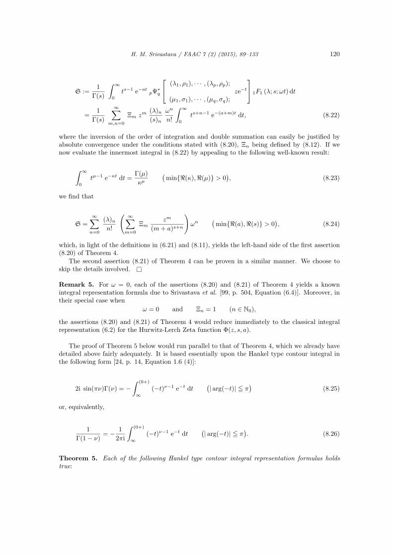
Proof. We find it to be convenient to denote by S the second member of the assertion (8.20) ofTheorem 4. Then, upon expanding the functions pΨ
∗q and 1F1 in series forms, we find that
H. M. Srivastava / FAAC 7 (2) (2015), 89–133 120
S :=1
Γ(s)
∫ ∞
0
ts−1 e−atpΨ
∗q
(λ1, ρ1), · · · , (λp, ρp);
(µ1, σ1), · · · , (µq, σq);ze−t
1F1 (λ; s;ωt) dt
=1
Γ(s)
∞∑m,n=0
Ξm zm(λ)n(s)n
ωn
n!
∫ ∞
0
ts+n−1 e−(a+m)t dt, (8.22)
where the inversion of the order of integration and double summation can easily be justified byabsolute convergence under the conditions stated with (8.20), Ξn being defined by (8.12). If wenow evaluate the innermost integral in (8.22) by appealing to the following well-known result:
∫ ∞
0
tµ−1 e−κt dt =Γ(µ)
κµ(minℜ(κ),ℜ(µ) > 0
), (8.23)
we find that
S =
∞∑n=0
(λ)nn!
( ∞∑m=0
Ξmzm
(m+ a)s+n
)ωn
(minℜ(a),ℜ(s) > 0
), (8.24)
which, in light of the definitions in (6.21) and (8.11), yields the left-hand side of the first assertion(8.20) of Theorem 4.
The second assertion (8.21) of Theorem 4 can be proven in a similar manner. We choose toskip the details involved.
Remark 5. For ω = 0, each of the assertions (8.20) and (8.21) of Theorem 4 yields a knownintegral representation formula due to Srivastava et al. [99, p. 504, Equation (6.4)]. Moreover, intheir special case when
ω = 0 and Ξn = 1 (n ∈ N0),
the assertions (8.20) and (8.21) of Theorem 4 would reduce immediately to the classical integralrepresentation (6.2) for the Hurwitz-Lerch Zeta function Φ(z, s, a).
The proof of Theorem 5 below would run parallel to that of Theorem 4, which we already havedetailed above fairly adequately. It is based essentially upon the Hankel type contour integral inthe following form [24, p. 14, Equation 1.6 (4)]:
2i sin(πν)Γ(ν) = −∫ (0+)
∞(−t)ν−1 e−t dt
(| arg(−t)| 5 π
)(8.25)
or, equivalently,
1
Γ(1− ν)= − 1
2πi
∫ (0+)
∞(−t)ν−1 e−t dt
(| arg(−t)| 5 π
). (8.26)
Theorem 5. Each of the following Hankel type contour integral representation formulas holdstrue:
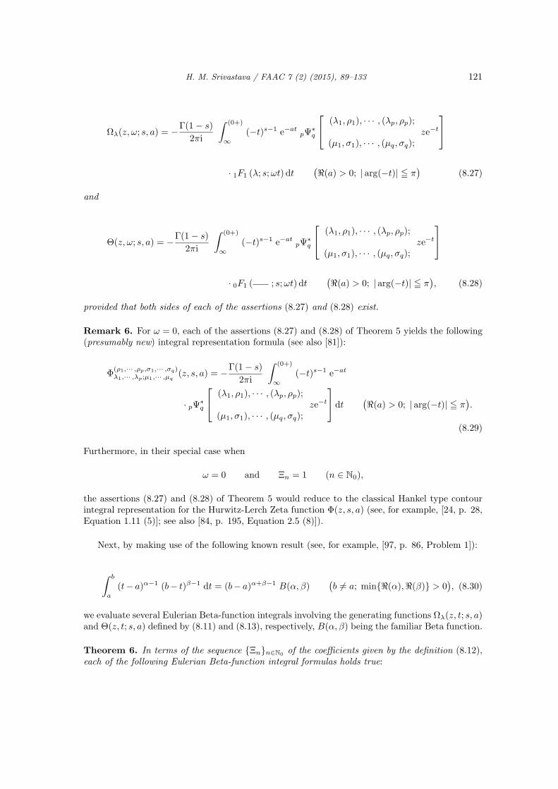
H. M. Srivastava / FAAC 7 (2) (2015), 89–133 121
Ωλ(z, ω; s, a) = −Γ(1− s)
2πi
∫ (0+)
∞(−t)s−1 e−at
pΨ∗q
(λ1, ρ1), · · · , (λp, ρp);
(µ1, σ1), · · · , (µq, σq);ze−t
· 1F1 (λ; s;ωt) dt
(ℜ(a) > 0; | arg(−t)| 5 π
)(8.27)
and
Θ(z, ω; s, a) = −Γ(1− s)
2πi
∫ (0+)
∞(−t)s−1 e−at
pΨ∗q
(λ1, ρ1), · · · , (λp, ρp);
(µ1, σ1), · · · , (µq, σq);ze−t
· 0F1 ( ; s;ωt) dt
(ℜ(a) > 0; | arg(−t)| 5 π
), (8.28)
provided that both sides of each of the assertions (8.27) and (8.28) exist.
Remark 6. For ω = 0, each of the assertions (8.27) and (8.28) of Theorem 5 yields the following(presumably new) integral representation formula (see also [81]):
Φ(ρ1,··· ,ρp,σ1,··· ,σq)λ1,··· ,λp;µ1,··· ,µq
(z, s, a) = −Γ(1− s)
2πi
∫ (0+)
∞(−t)s−1 e−at
· pΨ∗q
(λ1, ρ1), · · · , (λp, ρp);
(µ1, σ1), · · · , (µq, σq);ze−t
dt(ℜ(a) > 0; | arg(−t)| 5 π
).
(8.29)
Furthermore, in their special case when
ω = 0 and Ξn = 1 (n ∈ N0),
the assertions (8.27) and (8.28) of Theorem 5 would reduce to the classical Hankel type contourintegral representation for the Hurwitz-Lerch Zeta function Φ(z, s, a) (see, for example, [24, p. 28,Equation 1.11 (5)]; see also [84, p. 195, Equation 2.5 (8)]).
Next, by making use of the following known result (see, for example, [97, p. 86, Problem 1]):
∫ b
a
(t− a)α−1 (b− t)β−1 dt = (b− a)α+β−1 B(α, β)(b = a; minℜ(α),ℜ(β) > 0
), (8.30)
we evaluate several Eulerian Beta-function integrals involving the generating functions Ωλ(z, t; s, a)and Θ(z, t; s, a) defined by (8.11) and (8.13), respectively, B(α, β) being the familiar Beta function.
Theorem 6. In terms of the sequence Ξnn∈N0 of the coefficients given by the definition (8.12),each of the following Eulerian Beta-function integral formulas holds true:

H. M. Srivastava / FAAC 7 (2) (2015), 89–133 122
∫ η
ξ
(t− ξ)α−1 (η − t)β−1 Ωλ
(z, ω(t− ξ)γ (η − t)δ; s, a
)dt
= (η − ξ)α+β−1 B(α, β)∞∑
n=0
Ξnzn
(n+ a)s3Ψ
∗1
(λ, 1), (α, γ), (β, δ);
(α+ β, γ + δ);
ω(η − ξ)γ+δ
n+ a
(8.31)(
η = ξ; minℜ(α),ℜ(β) > 0; γ, δ > 0)
and
∫ η
ξ
(t− ξ)α−1 (η − t)β−1 Θ(z, ω(t− ξ)γ (η − t)δ; s, a
)dt
= (η − ξ)α+β−1 B(α, β)∞∑
n=0
Ξnzn
(n+ a)s2Ψ
∗1
(α, γ), (β, δ);
(α+ β, γ + δ);
ω(η − ξ)γ+δ
n+ a
(8.32)
(η = ξ; minℜ(α),ℜ(β) > 0; γ, δ > providedthatboth0
),
provided that both sides of each of the assertions (8.31) and (8.32) exist, the Fox-Wright function
3Ψ∗1 in (8.31) being tacitly interpreted as an H-function contained in the definition (6.26).
Proof. Each of the assertions (8.31) and (8.32) of Theorem 6 can be proven fairly easily by appealingto the definitions (8.11) and (8.13), respectively, in conjunction with the Eulerian Beta-functionintegral (8.30). The details involved are being skipped here.
Remark 7. In addition to their relatively more familiar cases when ξ = η − 1 = 0, variousinteresting limit cases of the integral formulas (8.31) and (8.32) asserted by Theorem 6 can bededuced by letting
limγ ↓ 0
or limδ ↓ 0
.
Several such very specialized cases of Theorem 6 as those that are indicated above can be foundin the recent works [10], [38] and [67].
The Eulerian Gamma-function integrals involving the generating functions Ωλ(z, t; s, a) andΘ(z, t; s, a) defined by (8.11) and (8.13), respectively, which are asserted by Theorem 7 below, canbe evaluated by applying the well-known formula (8.23).
Theorem 7. Let the function Φ∗µ(z, s, a) be defined by (6.11). Then, in terms of the sequence
Ξnn∈N0 of the coefficients given by the definition (8.12), each of the following single or doubleEulerian Gamma-function integral formulas holds true:
1
Γ(µ)
∫ ∞
0
tµ−1 e−κt Ωλ
(z, ωe−δt; s, a
)dt
= δ−µ∞∑
n=0
Ξnzn
(n+ a)sΦ∗
λ
(ω
n+ a, µ,
κ
δ
) (minℜ(κ),ℜ(µ),ℜ(δ) > 0
), (8.33)
1
Γ(µ)
∫ ∞
0
tµ−1 e−κt Θ(z, ωt; s, a) dt = κ−µ Ωµ
(z,ω
κ; s, a
) (minℜ(κ),ℜ(µ) > 0
)(8.34)
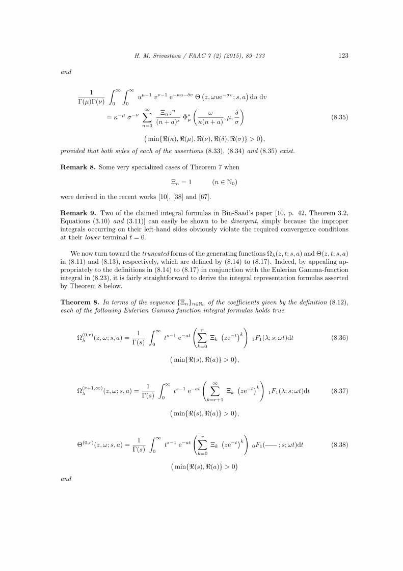
H. M. Srivastava / FAAC 7 (2) (2015), 89–133 123
and
1
Γ(µ)Γ(ν)
∫ ∞
0
∫ ∞
0
uµ−1 vν−1 e−κu−δv Θ(z, ωue−σv; s, a
)du dv
= κ−µ σ−ν∞∑
n=0
Ξnzn
(n+ a)sΦ∗
µ
(ω
κ(n+ a), µ,
δ
σ
)(8.35)
(minℜ(κ),ℜ(µ),ℜ(ν),ℜ(δ),ℜ(σ) > 0
),
provided that both sides of each of the assertions (8.33), (8.34) and (8.35) exist.
Remark 8. Some very specialized cases of Theorem 7 when
Ξn = 1 (n ∈ N0)
were derived in the recent works [10], [38] and [67].
Remark 9. Two of the claimed integral formulas in Bin-Saad’s paper [10, p. 42, Theorem 3.2,Equations (3.10) and (3.11)] can easily be shown to be divergent, simply because the improperintegrals occurring on their left-hand sides obviously violate the required convergence conditionsat their lower terminal t = 0.
We now turn toward the truncated forms of the generating functions Ωλ(z, t; s, a) and Θ(z, t; s, a)in (8.11) and (8.13), respectively, which are defined by (8.14) to (8.17). Indeed, by appealing ap-propriately to the definitions in (8.14) to (8.17) in conjunction with the Eulerian Gamma-functionintegral in (8.23), it is fairly straightforward to derive the integral representation formulas assertedby Theorem 8 below.
Theorem 8. In terms of the sequence Ξnn∈N0 of the coefficients given by the definition (8.12),each of the following Eulerian Gamma-function integral formulas holds true:
Ω(0,r)λ (z, ω; s, a) =
1
Γ(s)
∫ ∞
0
ts−1 e−at
(r∑
k=0
Ξk
(ze−t
)k)1F1(λ; s;ωt)dt (8.36)
(minℜ(s),ℜ(a) > 0
),
Ω(r+1,∞)λ (z, ω; s, a) =
1
Γ(s)
∫ ∞
0
ts−1 e−at
( ∞∑k=r+1
Ξk
(ze−t
)k)1F1(λ; s;ωt)dt (8.37)
(minℜ(s),ℜ(a) > 0
),
Θ(0,r)(z, ω; s, a) =1
Γ(s)
∫ ∞
0
ts−1 e−at
(r∑
k=0
Ξk
(ze−t
)k)0F1( ; s;ωt)dt (8.38)
(minℜ(s),ℜ(a) > 0
)and
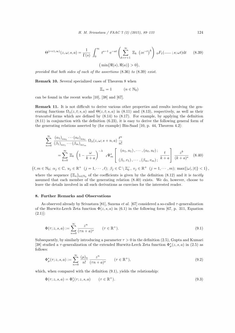
H. M. Srivastava / FAAC 7 (2) (2015), 89–133 124
Θ(r+1,∞)(z, ω; s, a) =1
Γ(s)
∫ ∞
0
ts−1 e−at
( ∞∑k=r+1
Ξk
(ze−t
)k)0F1( ; s;ωt)dt (8.39)
(minℜ(s),ℜ(a) > 0
),
provided that both sides of each of the assertions (8.36) to (8.39) exist.
Remark 10. Several specialized cases of Theorem 8 when
Ξn = 1 (n ∈ N0)
can be found in the recent works [10], [38] and [67].
Remark 11. It is not difficult to derive various other properties and results involving the gen-erating functions Ωλ(z, t; s, a) and Θ(z, t; s, a) in (8.11) and (8.13), respectively, as well as theirtruncated forms which are defined by (8.14) to (8.17). For example, by applying the definition(8.11) in conjunction with the definition (6.23), it is easy to derive the following general form ofthe generating relations asserted by (for example) Bin-Saad [10, p. 44, Theorem 4.2]:
∞∑n=0
(α1)nu1· · · (αℓ)nuℓ
(β1)nv1· · · (βm)nvm
Ωλ(z, ω; s+ n, a)tn
n!
=∞∑k=0
Ξk
(1− ω
k + a
)−λ
ℓΨ∗m
(α1, u1) , · · · , (αℓ, uℓ) ;
(β1, v1) , · · · , (βm, vm) ;
t
k + a
zk
(k + a)s(8.40)
(ℓ,m ∈ N0; αj ∈ C, uj ∈ R+ (j = 1, · · · , ℓ); βj ∈ C \ Z−
0 , vj ∈ R+ (j = 1, · · · ,m); max|ω|, |t| < 1),
where the sequence Ξnn∈N0 of the coefficients is given by the definition (8.12) and it is tacitlyassumed that each member of the generating relation (8.40) exists. We do, however, choose toleave the details involved in all such derivations as exercises for the interested reader.
8. Further Remarks and Observations
As observed already by Srivastava [81], Saxena et al. [67] considered a so-called τ -generalizationof the Hurwitz-Lerch Zeta function Φ(z, s, a) in (6.1) in the following form [67, p. 311, Equation(2.1)]:
Φ(τ ; z, s, a) :=∞∑
n=0
zn
(τn+ a)s(τ ∈ R+). (9.1)
Subsequently, by similarly introducing a parameter τ > 0 in the definition (2.5), Gupta and Kumari[38] studied a τ -generalization of the extended Hurwitz-Lerch Zeta function Φ∗
µ(z, s, a) in (2.5) asfollows:
Φ∗µ(τ ; z, s, a) :=
∞∑n=0
(µ)nn!
zn
(τn+ a)s(τ ∈ R+), (9.2)
which, when compared with the definition (9.1), yields the relationship:
Φ(τ ; z, s, a) = Φ∗1(τ ; z, s, a) (τ ∈ R+). (9.3)
H. M. Srivastava / FAAC 7 (2) (2015), 89–133 125
By looking closely at the definitions (9.1) and (9.2), in conjunction with the earlier definitions(6.1) and (6.11), respectively, we immediately get the following rather obvious connections:
Φ(τ ; z, s, a) =1
τsΦ(z, s,
a
τ
)or Φ (z, s, a) = τs Φ(τ ; z, s, aτ) (τ ∈ R+) (9.4)
and
Φ∗µ(τ ; z, s, a) =
1
τsΦ∗
µ
(z, s,
a
τ
)or Φ∗
µ (z, s, a) = τs Φ∗µ(τ ; z, s, aτ) (τ ∈ R+) (9.5)
Clearly, therefore, the definitions in (9.1) and (9.2) (with τ ∈ R+) are no more general thantheir corresponding well-known cases when τ = 1 given by the definitions in (6.1) and (6.11),respectively. Thus, by trivially appealing to the parametric changes exhibited by the connectionsin (9.4) and (9.5), all of the results involving the so-called τ -generalized functions Φ(τ ; z, s, a)and Φ∗
µ(τ ; z, s, a) can be derived simply from the corresponding (usually known) results involvingthe familiar functions Φ(z, s, a) and Φ∗
µ(z, s, a), respectively. Just for illustration of the trivialityassociated with such straightforward derivations, we recall the following sum-integral representationformula due to Lin and Srivastava [52, p. 729, Equation (20)] (see also [99, p. 494, Equation (2.6)]for the special case when k = 1):
Φ(ρ,σ)µ,ν (z, s, a) =
1
Γ(s)
k−1∑j=0
(µ)ρj(ν)σj
zj∫ ∞
0
ts−1 e−(a+j)t2Ψ1
(µ+ ρj, ρk) , (1, 1);
(ν + σj, σk) ;zk e−kt
dt (9.6)
(k ∈ N; minℜ(a),ℜ(s) > 0; σ > ρ > 0 when z ∈ C; σ = ρ > 0 when |z|1/k < ρ−ρ σσ
),
it being tacitly assumed that each member of (9.6) exists. Indeed, in the special case when
ρ = σ = ν = 1,
(9.6) yields the following sum-integral representation for the generalized Hurwitz-Lerch Zeta func-tion Φ∗
µ(z, s, a) involved in (6.11):
Φ∗µ(z, s, a) =
1
Γ(s)
k−1∑j=0
(µ)j(ν)j
zj∫ ∞
0
ts−1 e−(a+j)t2Ψ1
(µ+ j, k) , (1, 1);
(ν + j, k) ;zk e−kt
dt (9.7)
(k ∈ N; minℜ(a),ℜ(s) > 0; |z| < 1
)or, equivalently,
Φ∗µ(z, s, a) =
1
Γ(s)
k−1∑j=0
(µ)j(ν)j
zj∫ ∞
0
ts−1 e−(a+j)tk+1Fk
∆∗ (k;µ+ j) , (1, 1);
∆∗ (k; ν + j) ;zk e−kt
dt (9.8)
(k ∈ N; minℜ(a),ℜ(s) > 0; |z| < 1
),
where, for convenience, ∆∗ (n;λ) abbreviates the array of n parameters
λ
n,λ+ 1
n, · · · , λ+ n− 1
n(n ∈ N),
the array being empty when n = 0.
H. M. Srivastava / FAAC 7 (2) (2015), 89–133 126
Now, with a view to rewriting this last result (9.8) in terms of the τ -generalized Hurwitz-LerchZeta function Φ∗
µ(τ ; z, s, a) defined by (9.2), we simply make the following rather trivial parameterand variable changes:
a 7→ a
τ, t 7→ τt and dt 7→ τdt (τ ∈ R+)
and multiply the resulting equation by τ−s. By using the connection in (9.5), we are thus ledimmediately to the following sum-integral representation for the τ -generalized Hurwitz-Lerch Zetafunction Φ∗
µ(τ ; z, s, a) defined by (9.2) :
Φ∗µ(τ ; z, s, a) =
1
Γ(s)
k−1∑j=0
(µ)j(ν)j
zj
·∫ ∞
0
ts−1 e−(a+τj)tk+1Fk
∆∗ (k;µ+ j) , (1, 1);
∆∗ (k; ν + j) ;zk e−kτt
dt (9.9)
(k ∈ N; minℜ(a),ℜ(s) > 0; |z| < 1
),
provided that each member of the assertion (9.9) exists.In its obvious particular case when k = 1, the sum-integral representation (9.9) would simplify
at once to the following form [67, p. 311, Equation (2.2)]:
Φ∗µ(τ ; z, s, a) =
1
Γ(s)
∫ ∞
0
ts−1 e−at(1− ze−τt
)−µdt (9.10)
(ℜ(a) > 0; ℜ(s) > 0 when |z| < 1; ℜ(s) > 1 when z = 1
),
which obviously is equivalent to (and certainly not a generalization of) of the τ = 1 case derivedearlier by Goyal and Laddha [35, p. 100, Equation (1.6)].
Remark 12. The so-called τ -generalizations 2Rτ1 and 1R
τ1 of the Gauss hypergeometric function
2F1 and Kummer’s confluent hypergeometric function 1F1, respectively, which were used in theaforecited paper by Saxena et al. [67, p. 315], are obviously very specialized cases of the well-knownand extensively-investigated Fox-Wright function pΨq defined by (6.23). In fact, it is ealsily seenfrom the definition (6.23) that [67, pp. 315 and 317] (see also [2], [3] and [110])
2Rτ1(a, b; c; z) :=
Γ(c)
Γ(b)
∞∑n=0
(a)nΓ(b+ τn)
Γ(c+ τn)
zn
n!=
Γ(c)
Γ(a)Γ(b)2Ψ1
(a, 1) , (b, τ);
(c, τ) ;z
= 2Ψ
∗1
(a, 1) , (b, τ);
(c, τ) ;z
(|z| < 1; τ ∈ R+; c /∈ Z−0 ) (9.11)
and
1Rτ1(b; c; z) :=
Γ(c)
Γ(b)
∞∑n=0
Γ(b+ τn)
Γ(c+ τn)
zn
n!=
Γ(c)
Γ(b)1Ψ1
(b, τ) ;
(c, τ) ;z
= 1Ψ∗1
(b, τ) ;
(c, τ) ;z
(9.12)
(|z| <∞; τ ∈ R+; c /∈ Z−0 ).
Similar remarks and observations would apply equally strongly to the other τ -generalizations ofwell-known and extensively-investigated hypergeometric functions in one, two and more variables.
H. M. Srivastava / FAAC 7 (2) (2015), 89–133 127
We conclude our investigation by presenting a generalization of the sum-integral representationformula (9.6) due to Lin and Srivastava [52, p. 729, Equation (20)].
Theorem 9. The following sum-integral representation formula holds true:
Φ(ρ1,··· ,ρp,σ1,··· ,σq)λ1,··· ,λp;µ1,··· ,µq
(z, s, a) =1
Γ(s)
k−1∑j=0
p∏ℓ=1
(λℓ)jρℓ
q∏ℓ=1
(µℓ)jσℓ
zj
j!
∫ ∞
0
ts−1 e−(a+j)t
· p+1Ψ∗q+1
(λ1 + jρ1, kρ1) , · · · , (λp + jρp, kρp) , (1, 1);
(µ1 + jσ1, kσ1) , · · · , (µq + jσq, kσq) , (j + 1, k);zk e−kt
dt (9.13)
(k ∈ N; minℜ(a),ℜ(s) > 0
),
provided that each member of the assertion (9.13) exists.
Proof. First of all, in light of the following elementary series identity:
∞∑n=0
f(n) =k−1∑j=0
∞∑n=0
f(kn+ j) (k ∈ N),
we find from the definition (6.21) that
Φ(ρ1,··· ,ρp,σ1,··· ,σq)λ1,··· ,λp;µ1,··· ,µq
(z, s, a) = k−sk−1∑j=0
p∏ℓ=1
(λℓ)jρℓ
q∏ℓ=1
(µℓ)jσℓ
zj
j!
· Φ(kρ1,··· ,kρp,1,kσ1,··· ,kσq,k)λ1+jρ1,··· ,λp+jρp,1;µ1+jσ1,··· ,µq+jσq,j+1
(zk, s,
a+ j
k
)(k ∈ N). (9.14)
The assertion (9.13) of Theorem 9 would now emerge readily upon first appealing to the afore-mentioned known result due to Srivastava et al. [99, p. 504, Equation (6.4)] (see also Remark 7above) given by
Φ(ρ1,··· ,ρp,σ1,··· ,σq)λ1,··· ,λp;µ1,··· ,µq
(z, s, a) =1
Γ(s)
∫ ∞
0
ts−1 e−atpΨ
∗q
(λ1, ρ1), · · · , (λp, ρp);
(µ1, σ1), · · · , (µq, σq);ze−t
dt (9.15)
(minℜ(a),ℜ(s) > 0
)and then setting
t 7→ kt and dt 7→ k dt (k ∈ N).
Furthermore, in its special case when
p = 2 (λ1 = µ and ρ1 = ρ; λ2 = 1 and ρ2 = 1)
and
q = 1 (µ1 = ν and σ1 = σ),

H. M. Srivastava / FAAC 7 (2) (2015), 89–133 128
the general result (9.13) asserted by Theorem 9 can be seen to reduce immediately to the knownsum-integral representation formula (9.6) due to Lin and Srivastava [52, p. 729, Equation (20)].
Recently, by suitably modifying this last integral representation formula (9.15), Srivastava [79]introduced and systematicall investigated the various properties of a significantly more generalclass of Hurwitz-Lerch zeta type functions defined by
Φ(ρ1,··· ,ρp,σ1,··· ,σq)λ1,··· ,λp;µ1,··· ,µq
(z, s, a; b, λ) :=1
Γ(s)
∫ ∞
0
ts−1 exp
(−at− b
tλ
)
· pΨ∗q
(λ1, ρ1), · · · , (λp, ρp);
(µ1, σ1), · · · , (µq, σq);ze−t
dt, (9.16)
(minℜ(a),ℜ(s) > 0; ℜ(b) = 0; λ = 0
),
so that, obviously, we have the following relationship:
Φ(ρ1,··· ,ρp,σ1,··· ,σq)λ1,··· ,λp;µ1,··· ,µq
(z, s, a; 0, λ) = Φ(ρ1,··· ,ρp,σ1,··· ,σq)λ1,··· ,λp;µ1,··· ,µq
(z, s, a)
= eb Φ(ρ1,··· ,ρp,σ1,··· ,σq)λ1,··· ,λp;µ1,··· ,µq
(z, s, a; b, 0). (9.17)
In its special case whenp− 1 = q = 0 (λ1 = µ; ρ1 = 1),
the above definition (9.16) would reduce immediately to the following form:
Θλµ(z, s, a; b) :=
1
Γ(s)
∫ ∞
0
ts−1 exp
(−at− b
tλ
) (1− ze−t
)−µdt (9.18)
(minℜ(a),ℜ(s) > 0; ℜ(b) = 0; λ = 0; µ ∈ C
),
where we have assumed further that
ℜ(s) > 0 when b = 0 and |z| 5 1 (z = 1)
orℜ(s− µ) > 0 when b = 0 and z = 1,
provided, of course, that the integral in (9.18) exists. The function Θλµ(z, s, a; b) was introduced
and studied by Raina and Chhajed [63, p. 90, Equation (1.6)] and (more recently) by Srivastavaet al. [96]. An interesting further special case of the function Θλ
µ(z, s, a; b) arises when we setλ = µ = 1 and z = 1 in the definition (9.18). We thus find that
Θ11 (1, s, a; b) = ζb (s, a) :=
1
Γ (s)
∫ ∞
0
ts−1 exp
(−at− b
t
) (1− e−t
)−1dt, (9.19)
where ζb (s, a) is the extended Hurwitz zeta function defined in [13, p. 308]. Furthermore, in aseries of recent papers, Bayad et al. (see [8], [9] and [29]) introduced and studied the so-calledgeneralized Hurwitz-Lerch zeta function ζ(s, µ; a, z) of order µ, which they defined by (cf. [9, p.608, Equation (6)])
ζ(s, µ; a, z) :=Γ(µ)
Γ(s)
∫ ∞
0
ts−1 e−at
(1− ze−t)µ dt (9.20)
(ℜ(a) > 0; ℜ(s) > 0 when |z| 5 1 (z = 1); ℜ(s− µ) > 0 when z = 1
)
H. M. Srivastava / FAAC 7 (2) (2015), 89–133 129
or, equivalently, by (cf. [9, p. 608, Equation (7)])
ζ(s, µ; a, z) :=
∞∑n=0
Γ (µ+ n)
n!
zn
(a+ n)s . (9.21)
By comparing the definitions (6.11) and (9.21), it is easily observed that
ζ(s, µ; a, z) = Γ(µ) · Φ∗µ (z, s, a) and Φ∗
µ (z, s, a) =1
Γ(µ)ζ(s, µ; a, z). (9.22)
Clearly, therefore, Equations in (9.22) exhibit the fact that the generalized Hurwitz-Lerch zetafunction ζ(s, µ; a, z) of order µ, which was considered recently by Bayad et al. (see [8], [9] and [29])is only a constant multiple of the widely- and extensively-investigated extended Hurwitz-Lerch Zetafunction Φ∗
µ(z, s, a) defined by (6.11).For a detailed discussion of the various properties and results for, and the potential applications
of, the so-called λ-generalized Hurwitz-Lerch zeta function
Φ(ρ1,··· ,ρp,σ1,··· ,σq)λ1,··· ,λp;µ1,··· ,µq
(z, s, a; b, λ)
defined by (9.16), and also for their potential applications in Number Theory and GeometricFunction Theory in Complex Analysis and for some other statistical applications in probabilitydistribution theory, the interested reader should refer to the works by Srivastava et al. (see, forexample, [79], [85], [87], [86] and [88]).
Finally, in addition to the Open Problem mentioned in Section 7 (see also [19]), many otherproperties and results involving such important higher transcendental functions of (for example)Analytic Number Theory andMathematical Physics as the Riemann Zeta function ζ(s), the Hurwitz(or generalized) Zeta function ζ(s, a), and the Hurwitz-Lerch Zeta function Φ(z, s, a) as well asits various interesting extensions and generalizations, than those that we have considered in thisarticle, deserve to be investigated further.Acknowledgements. The present investigation was supported, in part, by the Natural Sciencesand Engineering Research Council of Canada under Grant OGP0007353.
References
[1] M. Abramowitz and I. A. Stegun (Editors), Handbook of Mathematical Functions with Formulas, Graphs, andMathematical Tables, Applied Mathematics Series 55, National Bureau of Standards, Washington, D.C., 1964;Reprinted by Dover Publications, New York, 1965 (see also [61]).
[2] A. Al-Zamel, On a generalized gamma-type distribution with τ -confluent hypergeometric function, Kuwait J.Sci. Engrg. 28 (2001), 25–36.
[3] I. Ali, S. L. Kalla and H. G. Khajah, A generalized inverse Gaussian distribution with τ -confluent hypergeo-metric function, Integral Transforms Spec. Funct. 12 (2001), 101–114.
[4] H. Alzer, D. Karayannakis and H. M. Srivastava, Series representations for some mathematical constants, J.Math. Anal. Appl. 320 (2006), 145–162.
[5] R. Apery, Irrationalite de ζ (2) et ζ (3), in Journees Arithmetiques de Luminy (Colloq. Internat. CNRS, CentreUniv. Luminy, Luminy, 1978), pp. 11–13, Asterisque 61, Soc. Math. France, Paris, 1979.
[6] T. M. Apostol, Introduction to Analytic Number Theory, Springer-Verlag, New York, Heidelberg and Berlin,1976.
[7] R. Ayoub, Euler and the Zeta function, Amer. Math. Monthly 81 (1974), 1067–1086.[8] A. Bayad and J. Chikhi, Reduction and duality of the generalized Hurwitz-Lerch zetas, Fixed Point Theory
Appl. 2013 (2013), Article ID 82, 1–14.[9] A. Bayad and S. Gaboury, Generalized Dirichlet L-function of arbitrary order with applications, Adv. Stud.
Contemp. Math. 23 (2013), 607–619.[10] M. G. Bin-Saad, Sums and partial sums of double power series associated with the generalized Zeta function
and their N -Fractional calculus, Math. J. Okayama Univ. 49 (2007), 37–52.[11] J. M. Borwein, D. M. Bradley and R. E. Crandall, Computational strategies for the Riemann Zeta function,
J. Comput. Appl. Math. 121 (2000), 247–296.
H. M. Srivastava / FAAC 7 (2) (2015), 89–133 130
[12] R. G. Buschman and H. M. Srivastava, The H-function associated with a certain class of Feynman integrals,J. Phys. A: Math. Gen. 23 (1990) 4707–4710.
[13] M. A. Chaudhry and S. M. Zubair, On a Class of Incomplete Gamma Functions with Applications, Chapmanand Hall (CRC Press Company), Boca Raton, London, New York and Washington, D.C., 2001.
[14] M.-P. Chen and H. M. Srivastava, Some families of series representations for the Riemann ζ (3), ResultateMath. 33 (1998), 179–197.
[15] J. Choi, Y. J. Cho and H. M. Srivastava, Series involving the Zeta and multiple Gamma functions, Appl. Math.Comput. 159 (2004), 509–537.
[16] J. Choi, D. S. Jang and H. M. Srivastava, A generalization of the Hurwitz-Lerch Zeta function, IntegralTransforms Spec. Funct. 19 (2008), 65–79.
[17] J. Choi and H. M. Srivastava, Certain families of series associated with the Hurwitz-Lerch Zeta function, Appl.Math. Comput. 170 (2005), 399–409.
[18] J. Choi and H. M. Srivastava, Explicit evaluation of Euler and related sums, Ramanujan J. 10 (2005), 51–70.[19] J. Choi and H. M. Srivastava, Series involving the Zeta functions and a family of generalized Goldbach-Euler
series, Amer. Math. Monthly 121 (2014), 229–236.[20] J. Choi, H. M. Srivastava and V. S. Adamchik, Multiple Gamma and related functions, Appl. Math. Comput.
134 (2003), 515–533.[21] D. Cvijovic and J. Klinowski, New rapidly convergent series representations for ζ (2n+ 1), Proc. Amer. Math.
Soc. 125 (1997), 1263–1271.[22] D. Cvijovic and H. M. Srivastava, Limit representations of Riemann’s Zeta function, Amer. Math. Monthly
119 (2012), 324–330.[23] A. Dabrowski, A note on the values of the Riemann Zeta function at positive odd integers, Nieuw Arch. Wisk.
(Ser. 4) 14 (1996), 199–207.[24] A. Erdelyi, W. Magnus, F. Oberhettinger and F. G. Tricomi, Higher Transcendental Functions, Vol. I, McGraw-
Hill Book Company, New York, Toronto and London, 1953.[25] A. Erdelyi, W. Magnus, F. Oberhettinger and F. G. Tricomi, Tables of Integral Transforms, Vol. II, McGraw-
Hill Book Company, New York, Toronto and London, 1954.[26] J. A. Ewell, A new series representation for ζ (3), Amer. Math. Monthly 97 (1990), 219–220.[27] J. A. Ewell, On the Zeta function values ζ(2k + 1), k = 1, 2, · · · , Rocky Mountain J. Math. 25 (1995), 1003–
1012.[28] S. R. Finch, Mathematical Constants, Encyclopedia of Mathematics and Its Applications, vol. 94, Cambridge
University Press, Cambridge, New York, Port Melbourne, Madrid and Cape Town, 2003.[29] S. Gaboury and A. Bayad, Series representations at special values of generalized Hurwitz-Lerch zeta function,
Abstr. Appl. Anal. 2013 (2013), Article ID 975615, 1–8.[30] M. Garg, K. Jain and S. L. Kalla, A further study of general Hurwitz-Lerch zeta function, Algebras Groups
Geom. 25 (2008), 311–319.[31] M. Garg, K. Jain and H. M. Srivastava, Some relationships between the generalized Apostol-Bernoulli
polynomials and Hurwitz-Lerch Zeta functions, Integral Transforms Spec. Funct. 17 (2006), 803–815.[32] J. W. L. Glaisher, On the history of Euler’s constant, Messenger Math. 1 (1872) 25–30.[33] M. L. Glasser, Some integrals of the arctangent function, Math. Comput. 22 (1968), 445–447.[34] R. W. Gosper Jr., A calculus of series rearrangements, in Algorithms and Complexity: New Directions and
Recent Results (J. F. Traub, Editor), pp. 121–151, Academic Press, New York, London and Toronto, 1976.[35] S. P. Goyal and R. K. Laddha, On the generalized Zeta function and the generalized Lambert function, Gan. ita
Sandesh 11 (1997), 99–108.[36] I. S. Gradshteyn and I. M. Ryzhik, Tables of Integrals, Series, and Products (Corrected and Enlarged edition
prepared by A. Jeffrey), Academic Press, New York, 1980; sixth edition, 2000.[37] P. L. Gupta, R. C. Gupta, S.-H. Ong and H. M. Srivastava, A class of Hurwitz-Lerch Zeta distributions and
their applications in reliability, Appl. Math. Comput. 196 (2008), 521–531.[38] R. K. Gupta and M. Kumari, Some results on a τ -generalized Riemann Zeta function, Jnanabha 41 (2011),
63–68.[39] E. R. Hansen, A Table of Series and Products, Prentice-Hall, Englewood Cliffs, New Jersey, 1975.[40] M. M. Hjortnaes, OverfØring av rekken
∑∞k=1
(1/k3
)til et bestemt integral, Proceedings of the Twelfth
Scandanavian Mathematical Congress (Lund; August 10-15, 1953), pp. 211–213, Scandanavian Mathemati-cal Society, Lund, 1954.
[41] A. A. Inayat-Hussain, New properties of hypergeometric series derivable from Feynman integrals. I:Transformation and reduction formulae, J. Phys. A: Math. Gen. 20 (1987), 4109–4117.
[42] A. A. Inayat-Hussain, New properties of hypergeometric series derivable from Feynman integrals. II: Ageneralization of the H-function, J. Phys. A: Math. Gen. 20 (1987), 4119–4128.
[43] D. Jankov, T. K. Pogany and R. K. Saxena, An extended general Hurwitz-Lerch Zeta function as a Mathieu(a,λ)-series, Appl. Math. Lett. 24 (2011), 1473–1476.
[44] S. Kanemitsu, M. Katsurada and M. Yoshimoto, On the Hurwitz-Lerch Zeta-function, Aequationes Math. 59(2000), 1–19.
[45] S. Kanemitsu, H. Kumagai and M. Yoshimoto, Sums involving the Hurwitz Zeta functions, Ramanujan J. 5(2001), 5–19.
H. M. Srivastava / FAAC 7 (2) (2015), 89–133 131
[46] S. Kanemitsu, H. Kumagai, H. M. Srivastava and M. Yoshimoto, Some integral and asymptotic formulasassociated with the Hurwitz Zeta function, Appl. Math. Comput. 154 (2004), 641–664.
[47] M. Katsurada, On Mellin-Barnes type of integrals and sums associated with the Riemann Zeta-function, Publ.Inst. Math. (Beograd) (Nouvelle Ser.) 62 (76) (1997), 13–25.
[48] M. Katsurada, Rapidly convergent series representations for ζ(2n + 1) and their χ-analogue, Acta Arith. 90(1999), 79–89.
[49] A. A. Kilbas, M. Saigo and J. J. Trujillo, On the generalized Wright functions, Fract. Calc. Appl. Anal. 5(2002), 437–466.
[50] A. A. Kilbas, H. M. Srivastava and J. J. Trujillo, Theory and Applications of Fractional Differential Equations,North-Holland Mathematical Studies, Vol. 204, Elsevier (North-Holland) Science Publishers, Amsterdam, Lon-don and New York, 2006.
[51] N. Koblitz, p-Adic Numbers, p-Adic Analysis, and Zeta-Functions, Graduate Texts in Mathematics, Vol. 58,Springer-Verlag, New York, Heidelberg and Berlin, 1977.
[52] S.-D. Lin and H. M. Srivastava, Some families of the Hurwitz-Lerch Zeta functions and associated fractionalderivative and other integral representations, Appl. Math. Comput. 154 (2004), 725–733.
[53] S.-D. Lin, H. M. Srivastava and P.-Y. Wang, Some expansion formulas for a class of generalized Hurwitz-LerchZeta functions, Integral Transforms Spec. Funct. 17 (2006), 817–827.
[54] W. Magnus, F. Oberhettinger and R. P. Soni, Formulas and Theorems for the Special Functions of Math-ematical Physics, Third Enlarged Edition, Die Grundlehren der Mathematischen Wissenschaften in Einzel-darstellungen mit besonderer Berucksichtingung der Anwendungsgebiete, Bd. 52, Springer-Verlag, New York,1966.
[55] A. M. Mathai, R. K. Saxena and H. J. Haubold, The H-Function: Theory and Applications, Springer, NewYork, Dordrecht, Heidelberg and London, 2010.
[56] Z. A. Melzak, Companion to Concrete Mathematics, Vol. I: Mathematical Techniques and Various Applications,John Wiley and Sons, New York, London, Sydney and Toronto, 1973.
[57] C. Nash and D. O’Connor, Ray-Singer torsion, topological field theories and the Riemann Zeta function ats = 3, in Low-Dimensional Topology and Quantum Field Theory (Proceedings of a NATO Advanced ResearchWorkshop held at the Isaac Newton Institute at Cambridge, U.K.; September 6-12, 1992) (H. Osborn, Editor),pp. 279–288, Plenum Press, New York and London, 1993.
[58] C. Nash and D. O’Connor, Determinants of Laplacians, the Ray-Singer torsion on lens spaces and the RiemannZeta function, J. Math. Phys. 36 (1995), 1462–1505.
[59] N. Nielsen, Handbuch der Theorie der Gammafunktion, Druck und Verlag von B. G. Teubner, Leipzig, 1906;Reprinted by Chelsea Publishing Company, New York, 1965.
[60] K. Nishimoto, C.-E Yen and M.-L. Lin, Some integral forms for a generalized Zeta function, J. Fract. Calc. 22(2002), 91–97.
[61] F. W. J. Olver, D. W. Lozier, R. F. Boisvert and C. W. Clark (Editors), NIST Handbook of MathematicalFunctions [With 1 CD-ROM (Windows, Macintosh and UNIX)], U. S. Department of Commerce, NationalInstitute of Standards and Technology, Washington, D. C., 2010; Cambridge University Press, Cambridge,London and New York, 2010 (see also [1]).
[62] D. Raducanu and H. M. Srivastava, A new class of analytic functions defined by means of a convolution operatorinvolving the Hurwitz-Lerch Zeta function, Integral Transforms Spec. Funct. 18 (2007), 933–943.
[63] R. K. Raina and P. K. Chhajed, Certain results involving a class of functions associated with the Hurwitz zetafunction, Acta Math. Univ. Comenianae 73 (2004), 89–100.
[64] V. Ramaswami, Notes on Riemann’s ζ-function, J. London Math. Soc. 9 (1934), 165–169.[65] S. G. Samko, A. A. Kilbas and O. I. Marichev, Fractional Integrals and Derivatives: Theory and Applications,
Translated from the Russian: Integrals and Derivatives of Fractional Order and Some of Their Applications(”Nauka i Tekhnika”, Minsk, 1987), Gordon and Breach Science Publishers, Reading, Tokyo, Paris, Berlin andLanghorne (Pennsylvania), 1993.
[66] R. K. Saxana, A remark on a paper on M -series [MR2401326 (2009b:26008)]. With an editorial note, Fract.Calc. Appl. Anal. 12 (2009), 109–110.
[67] R. K. Saxena, R. K. Gupta and M. Kumari, Integrals and series expansions of the τ -generalized Riemann Zetafunction, J. Indian Acad. Math. 33 (2011), 309–320.
[68] R. K. Saxena, T. K. Pog’any, R. Saxena and D. Jankov, On generalized Hurwitz-Lerch Zeta distributionsoccurring in statistical inference, Acta Univ. Sapientiae Math. 3 (2011), 43–59.
[69] M. Sharma, Fractional integration and fractional differentiation of the M -series, Fract. Calc. Appl. Anal. 11(2008), 187–191.
[70] M. Sharma and R. Jain, A note on a generalzed M -series as a special function of fractional calculus, Fract.Calc. Appl. Anal. 12 (2009), 449–452.
[71] H. M. Srivastava, A unified presentation of certain classes of series of the Riemann Zeta function, Riv. Mat.Univ. Parma (Ser. 4) 14 (1988), 1–23.
[72] H. M. Srivastava, Sums of certain series of the Riemann Zeta function, J. Math. Anal. Appl. 134 (1988),129–140.
[73] H. M. Srivastava, Certain families of rapidly convergent series representations for ζ (2n+ 1), Math. Sci. Res.Hot-Line 1 (6) (1997), 1–6 (Research Announcement).

H. M. Srivastava / FAAC 7 (2) (2015), 89–133 132
[74] H. M. Srivastava, Further series representations for ζ (2n+ 1), Appl. Math. Comput. 97 (1998), 1–15.[75] H. M. Srivastava, Some rapidly converging series for ζ (2n+ 1), Proc. Amer. Math. Soc. 127 (1999), 385–396.[76] H. M. Srivastava, Some simple algorithms for the evaluations and representations of the Riemann Zeta function
at positive integer arguments, J. Math. Anal. Appl. 246 (2000), 331-351.[77] H. M. Srivastava, Some formulas for the Bernoulli and Euler polynomials at rational arguments, Math. Proc.
Cambridge Philos. Soc. 129 (2000), 77–84.[78] H. M. Srivastava, Some generalizations and basic (or q-) extensions of the Bernoulli, Euler and Genocchi
polynomials, Appl. Math. Inform. Sci. 5 (2011), 390–444.[79] H. M. Srivastava, A new family of the λ-generalized Hurwitz-Lerch zeta functions with applications, Appl.
Math. Inform. Sci. 8 (2014), 1485-1500.[80] H. M. Srivastava, Riemann, Hurwitz and Hurwitz-Lerch Zeta functions and associated series and integrals, in
Essays in Mathematics and Its Applications (In Honor of Stephen Smale’s 80th Birthday) (Panos M. Pardalosand Th. M. Rassias, Editors), Springer-Verlag, Berlin, Heidelberg and New York, 2012, pp. 431-461.
[81] H. M. Srivastava, Generating relations and other results associated with some families of the extended Hurwitz-Lerch Zeta functions, SpringerPlus 2 (2013), Article ID 2:67, 1–14.
[82] H. M. Srivastava, Some τ -extensions of higher transcendental functions, J. Indian Acad. Math. 35 (2013),165–176.
[83] H. M. Srivastava and J. Choi, Series Associated with the Zeta and Related Functions, Kluwer AcademicPublishers, Dordrecht, Boston and London, 2001.
[84] H. M. Srivastava and J. Choi, Zeta and q-Zeta Functions and Associated Series and Integrals, Elsevier SciencePublishers, Amsterdam, London and New York, 2012.
[85] H. M. Srivastava and S. Gaboury, New expansion formulas for a family of the lambda-generalized Hurwitz-Lerchzeta functions, Internat. J. Math. Math. Sci. 2014 (2014), Article ID 131067, 1–13.
[86] H. M. Srivastava, S. Gaboury and B.-J. Fugere, Further results involving a class of generalized Hurwitz-LerchZeta functions, Russian J. Math. Phys. 21 (2014), 521-537.
[87] H. M. Srivastava, S. Gaboury and A. Bayad, Expansion formulas for an extended Hurwitz-Lerch zeta functionobtained via fracional calculus, Adv. Difference Equations 2014 (2014), Article ID 169, 1–17.
[88] H. M. Srivastava, S. Gaboury and R. Tremblay, New relations involving an extended multiparameter Hurwitz-Lerch zeta function with applications, Internat. J. Anal. 2014 (2014), Article ID 680850, 1–14.
[89] H. M. Srivastava, M. Garg and S. Choudhary, A new generalization of the Bernoulli and related polynomials,Russian J. Math. Phys. 17 (2010), 251–261.
[90] H. M. Srivastava, M. Garg and S. Choudhary, Some new families of generalized Euler and Genocchi polynomials,Taiwanese J. Math. 15 (2011), 283–305.
[91] H. M. Srivastava, M. L. Glasser and V. S. Adamchik, Some definite integrals associated with the Riemann Zetafunction, Z. Anal. Anwendungen 19 (2000), 831–846.
[92] H. M. Srivastava, K. C. Gupta and S. P. Goyal, The H-Functions of One and Two Variables with Applications,South Asian Publishers, New Delhi and Madras, 1982.
[93] H. M. Srivastava, D. Jankov, T. K. Pogany and R. K. Saxena, Two-sided inequalities for the extended Hurwitz-Lerch Zeta function, Comput. Math. Appl. 62 (2011), 516–522.
[94] H. M. Srivastava and P. W. Karlsson, Multiple Gaussian Hypergeometric Series, Halsted Press (Ellis HorwoodLimited, Chichester), John Wiley and Sons, New York, Chichester, Brisbane and Toronto, 1985.
[95] H. M. Srivastava, S.-D. Lin and P.-Y. Wang, Some fractional-calculus results for the H-function associatedwith a class of Feynman integrals, Russian J. Math. Phys. 13 (2006), 94–100.
[96] H. M. Srivastava, M.-J. Luo and R. K. Raina, New results involving a class of generalized Hurwitz-Lerch zetafunctions and their applications, Turkish J. Anal. Number Theory 1 (2013), 26–35.
[97] H. M. Srivastava and H. L. Manocha, A Treatise on Generating Functions, Halsted Press (Ellis HorwoodLimited, Chichester), John Wiley and Sons, New York, Chichester, Brisbane and Toronto, 1984.
[98] H. M. Srivastava, R. K. Saxena, T. K. Pogany and R. Saxena, Integral and computational representations ofthe extended Hurwitz–Lerch Zeta function, Integral Transforms Spec. Funct. 22 (2011), 487–506.
[99] H. M. Srivastava, R. K. Saxena, T. K. Pogany and R. Saxena, Integral and computational representations ofthe extended Hurwitz-Lerch Zeta function, Integral Transforms Spec. Funct. 22 (2011), 487–506.
[100] H. M. Srivastava and H. Tsumura, A certain class of rapidly convergent series representations for ζ (2n+ 1),J. Comput. Appl. Math. 118 (2000), 323–335.
[101] H. M. Srivastava and H. Tsumura, New rapidly convergent series representations for ζ (2n+ 1), L (2n, χ) andL (2n+ 1, χ), Math. Sci. Res. Hot-Line 4(7) (2000), 17–24 (Research Announcement).
[102] H. M. Srivastava and H. Tsumura, Certain classes of rapidly convergent series representations for L(2n, χ)and L(2n+ 1, χ), Acta Arith. 100 (2001), 195–201.
[103] H. M. Srivastava and H. Tsumura, Inductive construction of rapidly convergent series representations forζ (2n+ 1), Internat. J. Comput. Math. 80 (2003), 1161–1173.
[104] E. C. Titchmarsh, The Theory of the Riemann Zeta-Function, Oxford University (Clarendon) Press, Oxfordand London, 1951; Second Edition (Revised by D. R. Heath-Brown), 1986.
[105] F. G. Tricomi, Sulla somma delle inverse delle terze e quinte potenze dei numeri naturali, Atti Accad. Naz.Lincei Rend. Cl. Sci. Fis. Mat. Natur. (Ser. 8) 47 (1969), 16–18.
[106] H. Tsumura, On evaluation of the Dirichlet series at positive integers by q-calculation, J. Number Theory 48
H. M. Srivastava / FAAC 7 (2) (2015), 89–133 133
(1994), 383–391.[107] E. T. Whittaker and G. N. Watson, A Course of Modern Analysis: An Introduction to the General Theory
of Infinite Processes and of Analytic Functions; with an Account of the Principal Transcendental Functions,Fourth Edition, Cambridge University Press, Cambridge, London and New York, 1927.
[108] J. R. Wilton, A proof of Burnside’s formula for log Γ (x+ 1) and certain allied properties of Riemann’s ζ-function, Messenger Math. 52 (1922–1923), 90–93.
[109] E. Witten, On quantum gauge theories in two dimensions, Comm. Math. Phys. 141 (1991), 153–209.[110] N. O. Virchenko, S. L. Kalla and A. Al-Zamel, Some results on a generalized hypergeometric function, Integral
Transforms Spec. Funct. 12 (2001), 89?–100.[111] C.-E Yen, M.-L. Lin and K. Nishimoto, An integral form for a generalized Zeta function, J. Fract. Calc. 22
(2002), 99–102.[112] N.-Y. Zhang and K. S. Williams, Some series representations of ζ (2n+ 1), Rocky Mountain J. Math. 23
(1993), 1581–1592.[113] N.-Y. Zhang and K. S. Williams, Some infinite series involving the Riemann Zeta function, in Analysis,
Geometry and Groups: A Riemann Legacy Volume, Parts I and II (H. M. Srivastava and Th. M. Rassias,Editors), Part II, pp. 691–712, Hadronic Press, Palm Harbor, Florida, 1993.
[114] N.-Y. Zhang and K. S. Williams, Values of the Riemann Zeta function and integrals involving log(2 sinh θ2)
and log(2 sin θ2), Pacific J. Math. 168 (1995), 271–289.