1

Solvency Dynamics of an Evolving Agent-Based Banking System Model

Peter C. Anselmo*1,2

anselmo@nmt.edu

Max Planck1,3

mplanck@icasa.nmt.edu

New Mexico Institute of Mining and Technology

801 Leroy Place

Socorro, New Mexico 87801 USA

This Version: 18 December 2012

* Corresponding Author

1. Institute for Complex Additive Systems Analysis

2. Department of Management +1 575 835 5440

3. Department of Computer Science +1 575 835 5126

2

Abstract

We present a network model of a stylized banking system that is defined by

interbank claims and by riskier claims on a non-bank entity (NBE). Banks in

this balance-sheet-centered model are characterized by a simple, single-period

model of loan/borrowing decision-making behavior. Three different types of

banks are modeled: least-risky banks, middle-risk banks, and risky banks, and

the model also incorporates a bank of last resort (BLR) that offers interbank

loans and monitors the solvency of system banks. The network evolves as

claims are created and dissolved, and as defaults on both household loans and

loans by the NBE impact balance sheets and borrowing behavior. We propose

a balance-sheet-based measure of solvency, and the average of that measure is

used to assess overall system viability at each iteration of the model.

Betweeness centrality is measured for each bank/agent at each iteration, as is

community membership within the network; both measures evolve over time.

A simple measure of community average betweeness, the average of

betweeness centrality for all members of communities defined (at least

partially) by interbank liabilities, is used to assess the impact of communities

– and the degree of connectivity of member banks – on the average solvency

of the system. JEL Codes: C1, G2

Keywords: Banking system modeling and simulation; interbank loan network

modularity and community structure; community structure and system

solvency

1. Overview

We present a banking-system simulation model where bank balance sheets are simulated, a

solvency measure is estimated, and banks make daily decisions regarding borrowing/lending on

the basis of reserve requirements and daily capital flows. As part of the decision about loans

and/or investing in risky assets, in our simulation banks also make daily decisions about

participation – as borrowers or lenders – in the short-term interbank loan market. This granular

approach permits assessment of the structure and significance of individual banks with regard to

average system solvency in a relatively large and dynamic – with regard to interbank liabilities –

banking network.

The importance of individual banks to system solvency is assessed using an agent-based

simulation methodology that has been developed for the analysis of dynamic networks. This

3

methodology, which has been successfully applied in other network contexts (e.g., Planck, et. al,

[1]) may be used to “grow” a system of arbitrary size, and is also useful for studying the

dynamics associated with critical system variables and the removal of or instantaneous changes

to specific components of the system. The methodology allows us to, at each iteration of the

simulation, assess individual and community measures of network connectivity for each bank

and community to which they belong – regardless of whether they actually belong to a

community at any given point in the simulation process. The two measures are weighted

individual betweeness centrality and global community average betweeness, which is the average

of the weighted individual betweeness centrality for all members of a community at each

iteration of the simulation.

Our banking system model features banks that vary only by the degree of risky behavior that

they exhibit. In this version of the model, the degree of risky behavior is unchanging, and is

measured by the portion of balance-sheet assets allocated to non-household and on-topology

loans. Our relatively simple model of bank asset portfolio management is a non-optimization,

heuristic-based decision-making model (Anand, et. al. [2], Haldane and May [3]). This is in

contrast with more formal, equilibrium-based models of bank behavior (e.g., Allen, et. al. [4]

Cohen-Cole, et. al. [5]) that are implemented as the basis for studies of banking systems.

Our main purpose is to assess the impacts of individual bank centrality and the centrality of

communities of banks within a simulated network defined by interbank liabilities in the context

of the three levels of risk-taking in our model. We assess the impacts of centrality and

community on a measure of average system solvency that is based on balance-sheet elements.

Risks to the integrity of the banking system are assessed using the average solvency of all banks

in the system at any time t, and the risks to both individual banks and the system as a whole

(Eisenberg and Noe [6]; Elsinger, Lehar, and Summer [7]) can be dynamically assessed via this

measure.

We describe the development of the dynamic model/representation of the magnitude and

direction of interbank liabilities over time. One thing that differentiates our work is that we

develop the simulated network topology from scratch via a simple (but changeable) model of

bank behavior when overnight interbank loans are procured. We evolve a system of 300 banks

– and the topology of the network of interbank liabilities and investments in a risky non-bank

4

entity – over time in a simulation of daily changes in the topology of the interbank and non-bank

liability network. This network is allowed to evolve according to the ways that we model banks’

selection of sources of short-term interbank funds from the set of all bank/agents willing to

provide short-term funds to the would-be borrowing bank in question. In this context, our agent-

based model grounded in interbank liquidity-driven transactions that is similar in spirit to the

work of Giansante, et. al. [8].

The topology of the banking system is defined according to both interbank liabilities (Boss, et. al

[9]) and investment in risky alternative (that is, non-conventional loan) assets (Battiston, et. al.

[10]). Boss, et. al., who studied the Austrian banking system, found a low degree of separation –

few hops – between banks. They also provide examples of the notion of community structure,

one that we also include, albeit with a different measure of community (we use the measure

suggested by Newman [11]).

Battiston, et. al. model the effects of diversification on a banking network based on interbank

liabilities. They show that high levels of interbank connectivity can result in high levels of

systematic risk during times of financial distress. They suggest investigation of the effects of

clustering on systemic risk, and that is one of the objectives of this paper. We assess both

individual-bank betweeness centrality (Freeman [12]) in a modified way that is based on relative

weights (but not direction; see Gai,et. al. [13]) and community structure at each iteration of the

simulation. We then compute the average betweeness centrality for each community in the

network at each iteration, and this variable is the independent variable in regressions where the

average system solvency is the dependent variable.

Our model also includes a non-bank entity (NBE), which offers risky investments to banks that

are treated in the model as perpetuities. That is, claims on the NBE take the form of constant,

perpetual monthly returns on an investment with a randomly-generated expected return and

default probability. The NBE impacts the interbank loan network through defaults on individual

claims by investing banks,thereby providing idiosyncratic shocks to the system as cash-flow

problems caused by an individual non-bank entity default may propagate through the system.

As is the case on other works ([3], [13], [2], Anand, et. al. [14]), our model is a balance-sheet

model of interbank connectivity – as well as connectivity to a risky-investment providing non-

5

bank entity (NBE).Banks make daily decisions about on and off-topology loans – off-topology

loans take one of two forms; mortgage loans and higher-return credit-care loans, investment with

the NBE, or on or off-topology borrowing. Off topology borrowing is available through a bank

of last resort (BLR), which we also include in the model.

Thus, at each iteration of the model, the probability of a missed perpetuity payment from the

NBE for every individual investment for each bank is computed. This is also done with

individual simulated mortgage and what we refer to as credit-card loans – generally, household

loans, which are also assessed individually for missed payments (4 missed payments is

considered a default in this model), and individual loans are amortized and carried on bank

balance sheets at their amortized value. NBE investments are carried on bank balance sheets at

face value.

Networks form as banks resolve short-term reserve and solvency requirements in the overnight

loan market. We develop our network in the spirit of Rogers and Veraart [15], and Pokutta et. al

[16]; our dynamic simulation is similar in structure; our flexible (and, at this point, random)

model allows for “contagion” – in our case, cascading bank liquidity problems as measured by

individual and average system solvency – to be instantaneous and simultaneous. The model is

also similar to that of Barnhill and Schumacher [17] as we also specifically consider interbank

defaults (or partial defaults) and their impacts on the overall system in a dynamic simulation

environment. Unlike Barnhill and Schumacher, we assume that banks have full information

about an inquiring bank in the setting of very short-term interbank loan rates.

Like Mistrulli [18], Iyer and Peydro [19] and others, we allow individual banks in our simulated

system to fail. The BLR, in addition to its role as overnight lender – if banks choose to borrow –

also acts as a monitor of bank solvency computed from a balance-sheet-based solvency measure

that we introduce in the paper. The BLR can remove banks whose solvency levels drop below a

cutoff level for a prescribed number of days. Banks that are removed have their assets divided

among the four remaining most-solvent banks, and in this model bank liabilities are assumed by

the BLR.This is accomplished via simulated balance sheet data, so that the degree to which

failures cascade through the system is contingent on the strength of the surviving banks in the

community that included the failing bank. In addition to this bank-removal dimension, the

6

model also features mergers between randomly-selected banks throughout the course of the

simulation.

Risk in this model is essentially liquidity risk that propagates through the system, and is

measured as the average solvency of all banks remaining in the system at each iteration. We

discuss cash hoarding by banks facing liquidity problems, and present three hoarding scenarios.

Unlike Acharya and Skeie [20], bank hoarding in this model is based on current-period liquidity

shortfalls that are the result of randomly-occurring defaults off-topology loans or problems with

on-topology interbank claims.

The most likely on-topology liquidity shock will originate from an individual bank’s claim on

the NBE, which might then cascade through the system ([6], [7]). We do not consider

macroeconomic shocks or other events that may lead to bank runs (Shin [21]). Since our focus is

on our methodology, we also do not consider any sort of dynamic optimization model of bank

decision behavior. Rather, we present a simplified, single-period model of bank capital

allocation decisions that are driven by the desire to balance loan (and, in some cases, other

investing behavior) activity with the need to remain above a known solvency level.

The model is motivated by the need to consider interbank exposures and their associated risks for

both banks and the entire system. Our solvency measure is similar to the measure presented in

[13], and it is specifically connected to the simulated loan-decision process for each bank. We

compute and consider the average solvency measure in the context of individual bank

connectedness and average community connectedness based on simulated data generated from a

simple model of bank behavior regarding day-to-day operating decisions. This non-equilibrium

focus is more similar to simulation studies based on simulated networks [17], or simulation

studies based on real data [7].

The average of all remaining bank solvencies at each model iteration is the measure of system

viability. It is based on simulated balance-sheet entries that are updated at each tick, and it and

all measures are computed on a tick-by-tick, or (simulated) daily basis. In addition to the bank

consolidations that occur because of the insolvency condition that is enforced by the BLR, the

model also features random mergers that occur every 400 ticks.

7

Results for two network scenarios are presented. In the first case, interbank loans (as well as

loans from the BLR) are overnight in nature – loans must be repaid after one simulated day, or

tick. In the second case, interbank loans are repaid in 3 ticks, or simulated days. We find that

both individual betweeness centrality (IGB, which we call Individual Global Betweeness) and

the average IGB for all members of a given community at each timestep (GCAB; Global

Community Average Betweeness) are individually associated with average system solvency, but

the degree to which these measures are important for system solvency differs substantially by the

length of the overnight-loan payment period.

In the next section of the paper, we present our simple model of single-period, non-strategic bank

behavior. This model is based on simulated bank balance sheets, and those balance-sheet data

provide inputs for our model solvency measure. Bank borrowing and lending decisions are

described, and the ways in which these decisions lead to network topologies. A brief discussion

of our simple, non-optimization-based model of bank behavior that is based on a system with

three types of banks (conservative, moderate and risky), w here different behaviors are defined

by the degree to which banks invest with the NBE. Ways of measuring individual banks and

communities within network topologies are then discussed, and the regression model we use to

assess the impact of communities on average system solvency is discussed. This development of

the dynamic model of system topology is an important feature of this work.

We then present our hypotheses regarding the relationships between the connectedness of

community members in the context of the three classes of banks in our model. The results of the

regressions run on the simulated data are shown, and after a discussion we close the paper with a

conclusion and some ideas for further work.

2. The Model of Bank Behavior

Banks make decisions regarding off and on-topology loans to generate revenue (off-topology)

and cover reserve-requirements and liquidity shortfalls (on-topology). Off-topology loans in this

study are divided into two classes that we call mortgage loans and credit-card loans. All banks

divide available household-loan capital between these options at each timestep according to a

simple model that we present in this section. A third class of uses of funds, investment with the

non-bank entity (NBE), also exists. The degree of investment in the NBE is, as is described

8

below, the means by which we differentiate between three risk behaviors: least-risky, middle-

risk, and risky banks.

We also show how cash-hoarding and contagion can be explained in our model, and how our

model assumption about how interbank claims are prioritized leads to the potential for smaller

banks – as measured by interbank loan exposure – to be negatively impacted by community

membership.

2.1 A Single-Period Model of Bank Loan Decision Making

The reality for most banks is near-constant inflows and outflows to and from both the banking

network (the topology) and households and other non-banking network entities. Our model is

built around a discrete simplification of this process; on a simulated daily basis, the order of

discrete events in our model are as follows:

1. Cash in the form of loan payments, deposits (the change in deposits could be

negative) and un-loaned (to the network) cash from the preceding day arrives.

2. Payments are made as necessary on interbank obligations.

3. The resulting balance sheet enables a solvency computation at time t.

4. The net cash position is computed and compared with the reserve requirement on

deposits.

5. If interbank loans are needed to meet reserve requirements, those obligations are

incurred.

6. If no interbank loans are needed, then either cash is hoarded because of solvency

issues or investments and loans – including contributions to the interbank pool within

the individual bank – are made according to the bank’s behavior profile and several

other factors that we present below.

Steps 1-6 are repeated at each iteration of the system simulation model. Note that, in this model

of relatively conservative bank behavior, banks do not borrow to cover interbank liabilities and

(as we show below) will hoard cash if solvency levels are too low with regard to a standard

imposed by the Bank of Last Resort (BLR) combined with a safety margin selected by each

bank.

9

At each iteration (simulated time step), each bank in the system is faced with selection of

decision variables . For all banks remaining in the system at time t, the amount to

lend – both on and off the system topology - and the amount to borrow are determined.

In this version of the model, and . As we show below,

scenarios where both variables are equal to 0 are possible.

We assess the daily financial well-being of I individual banks, as well as the overall health of the

system, using our model-based solvency measure:

(1)

where denotes all other banks remaining in the system, and k denotes off-topology loans

(which are balance-sheet assets A) in the form of mortgages, credit cards, and other conventional

bank assets. Financial relations with the non-bank entity are considered as on-topology assets

in this model. The subscript C denotes cash.The letter L denotes on-topology liabilities, which

are overnight obligations to other banks and/or the bank of last resort (BLR). The model

in (1) is very similar to the liquidity condition in [13]. Their model contains provisions for repo

assets and liabilities (and associated haircut provisions), which are not part of our simulation

model. Elimination of the haircut variables by setting them equal to zero in the model in [13]

results in a model that is very close to what we propose in (1).

Their model also contains a provision for withdrawal of a fraction of interbank deposits because

of contagion-inspired liquidity hoarding. We do not explicitly consider this as part of the

solvency model. However, bank cash hoarding that results in either late payment or default on

individual liabilities will impact the measure in (1) and subsequent lending decisions as banks

try to maintain adequate solvency levels. Liquidity hoarding that leads to defaults on interbank

loans therefore impacts connected-bank solvency, and thereby the decision regarding .

We therefore can model similar network-driven contagion effects; our model considers

contagion as a dynamic factor and contagion impacts can be seen in the aggregate average

solvency (as well as individual bank solvency) measure.

We refer to as a “model” solvency measure because of its dependence on bank decision

variables and randomly-fluctuating deposits that drive the cash reserve requirement. Key

10

balance-sheet components missing from this formulation are fixed assets (aka property, plant,

and equipment), long-term debt, and stockholders’ equity. For many banks, the asset side of the

balance sheet is largely captured by the assets in the formulation, as long-term non-fixed

assets will largely be represented by off-topology loans .

On the liabilities side, current liabilities – with the exclusion of accounts payable – are

represented by the denominator in the formulation. For banks with little or no long-term

debt, the denominator largely represents the liability side of the balance sheet. Cash ( is net

of costs, and solvencies greater than 1 along with the presence of fixed assets and goodwill and

the non-presence of long-term debt might be sufficient for positive equity to exist. Shareholder

equity is not represented in (1), though solvencies greater than 1 are obviously desirable and we

use a solvency cutoff (for dissolution purposes by the BLR; this is a modeler-specified variable

in the simulations) of 1.05 in the simulations we ran. A summary of model variables and their

values used in the simulations discussed in this paper is presented in Table 1.

<< Please Insert Table 1 About Here in black and white >>

The periodic across-banks average of this solvency measure serves as our measure of system

stability and viability, as banks attempt to maintain solvency levels above the cutoff of 1.05

established by the BLR. The solvency measure also allows the impact of the BLR cutoff on

bank-decision making (as specified below) at each interval to be measured directly. The way

that banks specify the decision variable pair in our model is presented next.

Define as changes to deposits and total liabilities at the beginning of time t

respectively. Then, total net inflows to any bank at the beginning of time t are modeled as

(2)

Where denotes unused cash allocated for interbank loans from the preceding period, is

the share of cash allocated to overhead expenses1, and denotes claims from other banks –

including claims that were not paid in previous periods2 – that are due at time t. Total on-

1 Table 1 contains descriptions and values for the simulation variables presented in this paper.

2 Unpaid, past-due claims from other banks are prioritized for payment. This point is discussed below

in section 4.2.

11

topology, interbank claims due to be settled by bank i at time t, . More about ,

the amount allocated to an interbank pool by each bank at time t, is presented below in this

section of the paper.

Negative net inflows ( are possible in this model, though this will be generally due to

positive net inflows that are offset by interbank obligations as

. The result of this situation will be

borrowing in the current period, as we show below. If net inflows augmented by cash are not

sufficient to cover current-period interbank-network obligations, that is if

, then some payments will be missed – and

interbank liquidity contagion may occur. The degree to which contagion will propagate through

the system will be determined by the solvency status of banks whose claims on bank i are not

met at time t. We discuss this point in some detail later in this section of the paper.

On-topology loan payments for any bank j to bank ithat are due at time t are determined as

(3)

with q denoting the periodic interbank rate for each bank j for which bank i has a claim at time t.

With regard to the solvency expression in (1), The sum of payments is positive for interbank

inflows, and is negative (or zero) for individual interbank outflows with respect to bank i.

With respect to the balance sheet, note that will be reduced by each payment , and the

interbank asset will also change as for each payment received at time t from

any bank j.

Off-topology payments for each loan k held by bank i are

(4)

where the 0 subscript denotes the initial value of the off-topology loan to customer k, and r is the

periodic rate; n is the number of periods for the loan. Note that we are concerned with actual

inflows in the form of loan payments and interbank claim settlements.

12

Defaults and/or missed payments are considered separately using the model presented below,

and the balance sheet is updated using only actual bank inflows. As was the case for the

interbank asset, the household loan balance sheet item, , is changed as each loan is amortized

when each payment is made. Thus, for all k loans with payments at time t (denoted by ),

and, for all household loans, .

We define as the 8% reserve requirement imposed on most US banks. F denotes

the (known) solvency cutoff (we used a value of 1.05, as mentioned above) imposed by the BLR

on the system, and (in this model, at every iteration of the simulation) is the

added safety margin that is a decision variable for all banks. Thus, banks will lend based on the

constraint that .

Examination of (1) leads to the conclusion that banks do not borrow in the interbank market to

increase liquidity in this model. Borrowing increases both cash (by increasing ) and

liabilities (via a new or increased value) by the amount of the claim. Thus, in this single-

period bank-decision model, borrowing actually decreases solvency at the next tick for values

greater than 1. Banks in this model therefore use other methods to increase solvency, through

cash hoarding (a short-term measure) and, more conventionally, making loans.

Therefore, the first step of the bank-decision process is determination of whether there is a need

to borrow in the interbank market. Since banks do not increase liquidity in the interbank market,

this is done by assessing periodic inflows in light of reserve requirements and any projected

liquidity issues in the next period:

(5)

with actual borrowing occurring if in this model. If , then no borrowing or

lending occurs at that time t. In the event that , lending (both on and off-topology) is an

option for bank i. In that case determination of is the next step, and in our model is the

phase in the decision-making process where next-period (t+1) solvency and connected-bank

outflowsare considered. denotes the expected on-topology outflows for the subsequent tick:

(6)

13

Note that are known at time t, and banks are effectively planning to meet all on-

topology, interbank obligations at time t+1.

Banks in this model are cognizant of the ability of the BLR to close them if solvency levels

remain at or below a cutoff level F (as noted above, F= 1.053 for the simulations discussed here)

for some period of time (in this case, the time period is 180 ticks). As noted above with regard to

F, we include a safety margin that banks attempt to maintain when making the periodic

lending decision. The modeler-specified value was used for all banks and all

simulations.

If and , then

(7)

At each time interval t for which , banks must decide whether and how to allocate funds

to the on and off-topology credit markets. In the event that , the bank must select

parameters , , and , which are the portion of allocated to loans to the NBE and the

proportion ( of allocated to less-risky mortgage loans – as opposed to more-

risky (but not as risky as the NBE) credit-card loans, and the proportion , of the non-

mortgage, non-NBE pool to be allocated to (relatively risky household) credit card loans. The

amount is the allocation to the interbank pool for any bank at time t. In general,

and . The allocation share of to the interbank

pool, given that there is no hoarding and that is for all banks.

Values for , , and are maintained at constant levels in the simulations, and these values

are summarized in Table 1.

It is the parameter that determines the behavioral classification of banks in this model.

Specifically,

Least-Risky Bank

Medium-Risk Bank

3 For the purpose of initialization of the simulation, we use a value of F = .97 that is in effect until the

average solvency measure stabilizes – usually after about 350 ticks. After that point, F = 1.05.

14

Risky Bank

These values remain constant for all banks. Thus, a least-risky bank never invests with the NBE,

and a risky bank always invests with the NBE when .

2.2 Solvency Contagion and Cash-Hoarding

In this model, contagion is a function of solvency, particularly if a missed payment or default

from any loan – whether an interbank claim or a household loan – causes a bank’s solvency

to fall below the sum of the solvency cutoff and the bank’s own additional factor . Thus,

if and/or at time t. Rather than lending,

banks will hoard cash in order to increase solvencies; the amount of the individual hoard given

and is, in this model, based on Thus, banks will either hoard some or

all inflows (if ) or lend that amount proportionally among households and other banks.

Note that hoarding may occur for several periods after a liquidity interruption as banks

incrementally return to targeted liquidity levels.

When a delinquency occurs that is sufficient to cause , one of three actions will be

taken by bank i. Either interbank borrowing in the amount of , hoarding in the amount of

or hoarding in the amount of will occur. In all cases, lending activity will be reduced or

halted by the bank in question until, at some time in the future, .

Each of the three situations for any bank i following the liquidity event may result in different

contagion and hoarding scenarios, and the strength of the bank – in the form of vis-à-vis

after the liquidity event – can be seen as a key factor for interbank contagion. In the first

instance, where the liquidity event causes the bank to borrow to meet reserve requirements,

indicates that bank i will borrow to cover current (but not next-period) liabilities. If there

are insufficient funds in the interbank market at the best interest rate on offer, the bank will go to

the BLR for funding4. However, as noted above, borrowing in the current period to cover

current interbank obligations decreases solvency, and banks that are consistently borrowing to

cover current interbank loans will find themselves in a death spiral resulting in increasing

interbank liabilities and, eventually, insolvency.

4 This point is the topic of section 4.1.

15

If liquidity events are small enough so that, when one occurs, then two other scenarios

for the bank in question exist and are defined by the value of . In the first, . In this

case, there will be no lending activity and – since – the anticipated shortfall is with

regard to . Thus the amount will be hoarded. If , then the bank will not do

any additional borrowing and there will be no new impacts on the network. On the other hand, if

, then additional borrowing may occur, there may be missed interbank payments, and

the death spiral could begin. At a minimum, missed interbank obligations would lead to

contagion as described here in terms of disruptions in bank lending activity that could lead to the

death spiral of borrowing in one period and in the next.

As noted above, hoarding in the amount of can also occur if > 0. In this case, hoarding

could be due to the liquidity event’s negative impact on solvency, but contagion will not occur

until the bank finds itself in the distress scenario where constant borrowing leads eventually to

liquidity events at connected banks. Note that, because expected next-period obligations are part

of the computation, banks will not borrow to meet future obligations, but will borrow based

on periodic net inflows and the reserve requirement. In the event that a delinquency does not

cause , the bank will proceed with it’s normal decision processes, but with a

weakened and more-vulnerable solvency position.

We recognize that this is a fairly simplistic model of bank behavior, and it reflects our interest in

utilizing a simple, balance-sheet based model of bank loan/borrowing decision making to

develop our dynamic interbank (and bank-NBE connections) network. As we show below, this

model enables us to draw some interesting inferences from our regression studies of the

importance of bank connectivity and connectivity within communities for average system

solvency.

3. Loan Default Probabilities

At each point in the simulation, the risk of a payment default is computed for each appropriate

loan. The term appropriate loan refers to the idea that mortgage, credit card, and risky loans are

scheduled for simulated monthly payments – or a payment every 30 ticks. Once the simulation

has run for several hundred ticks, there are generally loans each tick for each bank that each need

to be assessed to determine whether a payment is missed.

16

The probability of a missed payment for any loan depends on loan interest rates r and is

computed from the following:

(8)

In 8, and are parameters that are specific to each of the two loan types – mortgage and

credit-card, as well as investment in the NBE. The constant risk of default at any time t is

increasing in r, which differs between the three types of off and on-topology investments

available to banks, but is constant for each loan throughout the simulation.

Thus, for each individual loan/investment, we have a set that defines , the

probability of a missed loan/investment payment, for each asset. For mortgage loans,

. For credit-card loans, = , and for

NBE investments, = where , a bank’s return rate on each

investment j, is uniformly distributed over the interval (.2, .4).

The rates r for all credit-card and mortgage loans for all banks remain fixed throughout all

simulations (this is another modeler decision variable that can be easily modified), while the

expected return from NBE investments is computed individually for each investment and tracked

throughout the simulations.

4. Dynamic Model Topologies

In this section, we specifically describe how we model interbank borrowing and, in the event of

insufficient funds to meet all obligations at any point in time, payback hierarchies. We start with

a general description of the problem of selection of a lender and our simple model in this context.

Then we present a brief discussion of the model of payback hierarchies, where banks select

banks to be repaid when there are insufficient funds to repay all obligations at any point in time.

4.1 Interbank Borrowing

Banks randomly select interbank loans based on quotes received from banks offering to loan in

the interbank market at each time step. The topology evolves as banks enter into and fulfill loan

obligations, which define the topology in terms of directed edges (in the direction of the lending

entity) when overnight loans exist and dissolved edges when the obligations are fulfilled by the

17

borrowing bank. Banks seeking to borrow in the interbank market receive rate quotes from all

other banks for which . These banks will offer bank i a quote . As we

show below, all quotes are organized into same-rate categories, which can then be parsed by any

bank i where the criterion is the magnitude of vis-à-vis . If there are no reasonably-

priced loans available in the overnight market, banks in this model turn to the BLR, which offers

overnight rates at the initial, starting rate . We assume that banks are reluctant to

access the BLR for interbank borrowing – because of information issues and the fact that, in our

model, the BLR will eliminate a bank that has missed overnight loan payments – even though the

BLR rate may be lower than other rates on offer at any time t.

We define in terms of interbank claims between banks i and j at the end of iteration t.

Specifically,

(9)

We represent a liability – one bank borrowing from another – as -1, with the corresponding claim

as a value of 1. = 0 if there is no connection between banks at time t.

As noted above, banks for which are assumed to parse the universe of all other banks to

find the interbank rate on offer, along with the amount allocated for interbank lending

for each bank. Note that will be true for banks for which or or

.

The result of the query of all other banks will be J pairs. A bank with will

randomly choose between the best rates available, and will group offering banks based on quoted

interbank rates at time t. This results in the formation of different classes of loan alternatives that

are determined by rates. Define as the best rate available at time t, as the next-best rate

available at time t, and so on. Then:

18

…..

for all m rates quoted in the interbank market at time t.

At the start of the simulation, m = 1 and all banks offer the same interbank rate. This overnight

rate is initially set at the BLR rate of If a bank defaults on an overnight loan, the

lending bank will raise the overnight rate for that bank by a uniformly distributed amount

. Obviously, as the simulation progresses and banks default on

each other, the number of different available rates m and rate classes across the simulated

banking system will increase.

In this model, interbank rates can only stay the same or increase. While it is possible within the

existing model framework to allow for changes to the base rate and/or to allow banks to reduce

rates for banks with long periods without a default, those factors are not included in the current

model.

We also assume that borrowing banks are somewhat interested in disguising the size of their

needed interbank borrowings at any time, and that, as mentioned above, borrowing from the

BLR at the initial interbank rate is not the preferred option for banks. Therefore we make a

modeling assumption that banks will attempt to spread their interbank overnight borrowing

activity among several banks (with the same low rate, of course) at any point in time. For the

purposes of the model presented here, we assume that banks prefer to borrow in equal

proportions from 3 banks, provided that there are 3 banks with the lowest rate on offer that also

have enough cash allocated to overnight borrowing. Within rate classes, if more than the

required number of banks (with respect to the borrowing bank i) have sufficient pool allocations,

the selection of lending banks is random.

Within each rate category the number of banks offering interbank loans at time t is defined as ,

with where is the total number of banks remaining in the system at time t. Note

that, as interbank loans are made within a given timestep, is constantly updated as individual

bank loan pools are reduced or utilized.

19

Another way of seeing this is to note that, in this model, all banks with sufficient funds to lend

will allocate a portion of those funds for offer to the interbank pool. As shown above in (2),

these funds may or may not be successfully consumed by borrowing banks at any timestep.

During the process, multiple borrowing banks may access an individual bank’s pool, and the size

of the pools and the number of remaining banks with sufficient pool assets within each rate

category is tracked within (and, of course, between) timesteps.

Borrowing banks parse the first rate class, and if there are more than 3 qualifying banks, the

actual 3 banks are randomly selected. If the first rate class does not contain sufficient candidate

banks for bank i, but does contain 1 or 2 sufficient banks, these banks will be selected and the

remaining lending bank(s) are selected from the next rate class. This process will iterate through

all rate classes until the loan is attained by the borrowing bank. If there are not a sufficient

number of banks meeting the loan criteria, the loan is realized – in part or wholly – via the BLR.

The probability that an interbank loan is made, that is for a borrowing bank and

for the corresponding lender, is, within each rate class a function of whether an

interbank claim already exists between bank i and j, whether bank j offers sufficient interbank

pool assets , and whether the borrowing bank has met its current borrowing target.

We define as the number of interbank loans made by bank i at any point in the

process of selecting interbank loans at time t.

Thus, for banks within the best rate class

(10)

if there are fewer qualifying banks in the pool than there are individual loans accepted by bank i

at time t,

(11)

For the next rate class, ,

(12)

20

with

(13)

and so on as bank I systematically considers each rate class according the rates on offer.

If or or then for all system banks.

In cases where for a selected lending bank, the amount borrowed by bank i will

be and the remainder – either ( after the most recent loan at time t) or

( – will be sought from other qualifying banks. As noted earlier, the BLR will fill any

outstanding borrowing requests once the entire set of offering banks is parsed – and the

borrowing bank will risk BLR shutdown if the loan is not repaid.

Naturally, when an overnight loan is repaid, = 0 for the loan in question, and the topology

continues to evolve as the edge between banks i and j is removed: .

While borrowing is an evident critical factor in network formation, removal of network arcs by

settling interbank claims is also critical as the banking network evolves. In the next section we

discuss how we modeled this feature of the problem in light of the notion that the change in the

cash position at time t might not be sufficient to pay all claims at time t+1.

4.2 Payment Hierarchies

At each model time step, banks are obligated for all on-topology loans due at that time. In this

paper, these are either overnight or 3-day loans. All topology claims will be settled if there is

sufficient cash at time t, that is if

where denotes a liability for bank i that is due in the current period – which, in this model, was

incurred either at time t-1 or time t-3 or is past due, having been incurred at time t-s; with s>1 in

the overnight repayment case or s>3 in the case of the 3-day payback model.

21

In the event that , some, but not all current on-topology obligations will

be met. Interbank claims must be prioritized, and in this model we do that based on past-due

status and size. Two distinct classes of interbank liabilities are possible: those that are past-due

and those that are current. In the case of past-due liabilities – these are, of course, potentially

contagion-inducing liabilities – claims are ordered for settlement based on the length of time they

have been past-due. All past-due claims have payment precedence over current (that is, due in

the current time period) interbank liabilities, which are prioritized based on size.

For past-due liabilities, the largest outstanding liability is paid first. Then, for current interbank

liabilities, the largest claim is settled first, followed by the next-largest, and so on until

. As we note above, this condition will result in both defaults on claims due in the next

period as well as borrowing to cover reserve requirements.

The vector of topology claims for bank i at time t, , where

is the time-ordered vector of past-due liabilities and the ordered-by-size vector of current-

period interbank liabilities is written as

where , , and so on. In the event that there are equally-late claims, they are

ordered by size, and equally-sized current liabilities are settled randomly if there are not

sufficient funds to settle both.

This establishes the payment hierarchy in the model: once late claims are paid, the bigger

obligation is always paid and, if there is sufficient remaining cash, then the next one is paid, and

if there is sufficient cash the next one is paid, and so on until either or all current

claims are settled. Naturally, as claims are settled, the corresponding edge in the network is

eliminated, and unpaid claims are prioritized for payment in the next period.

22

Once the interbank and NBE claim network has been established, we need to establish measures

of system and individual-bank connectivity. For this we use the well-known betweeness

centrality measure, which is the basis for the next section.

4.3 Connectivity and Modularity Measures

The well-known betweeness centrality measure is weighted by the relative magnitude of the

edges in the topology for each bank. This allows for both modified betweeness centrality (we

call this measure individual global betweeness, or IGB) and the average of modified betweeness

centrality for banks within a community (we refer to this measure as global average community

betweeness, or GACB) measures that specifically incorporate (and are modified according to)

the sizes of interbank exposures. The Brandes [22] method is determined to determine the

weighted betweeness centrality for each surviving bank at each time step.

Following [11] and [12], the modified measure of betweeness centrality at time t is modified by

relative weight as follows:

(13)

Where denotes shortest paths between banks j and k, and also shortest paths between j and k

that go through bank i. Weights are defined as the relative claim on bank j by bank i at time t:

(14)

Note that the above relative weight measure is defined in terms of the directionality of claims,

while shortest paths in the equation above are not measured with directionality in mind. For any

connection between banks i and j, happens when and there is a

directional arrow pointing from bank i to bank j that represents the claim on i by j.

Global community average betweeness (GCAB) is the average of the betweeness centrality

measures for all banks within a community at time t. Communities are determined at each

time using the method described in [11]. As shown in Figures 1a and 1b, once the simulated

interbank networks stabilize, the number of communities varies according to the experiment in

question. Thus,

23

(15)

Where denotes the number of banks in community at time t. Note that all members of

community at time t will have the same GCAB measure regardless of their differing IGB

measures, and this measure will change as network topologies change.

<< Please Insert Figures 1a and 1b About Here in color in web and print versions >>

When the number of communities is equal to the number of banks in the system, there are no

edges between banks or between banks and the NBE. No bank is part of a multi-bank

community, and all GCAB measures are equal. For the purposes of the defining the GCAB

regression variable, all banks have a GCAB measure of 0 in this instance5.

As the number of communities decreases, the number of edges defining the network (generally)

increases, and the network becomes defined. Generally, as the number of communities shrinks

the network becomes relatively more dense, and, perhaps, more vulnerable to individual-bank

solvency issues.

Examples of dynamic topologies for three consecutive ticks in a banking-system simulation

based on our model can be seen in Figures 2-4. These are taken from another of our banking-

system simulation papers that features 30 banks and overnight repayment requirements on

interbank loans and loans from the BLR. These topologies are included in this paper to illustrate

the notion of dynamic community membership because of the obvious ease of seeing

communities within a 30-bank topology instead of a 300-bank topology.

<< Please Insert Figures 2-4 About Here in color in web and print versions >>

The dynamic nature of community formation, membership and claims may be seen by

examination of Figures 2-4. The number of unconnected banks varies (from 4 to 3 to 4), the

number of communities with multiple members varies (from 6 to 6 to 4), and – as may be seen

5 In the actual data collection process, = -1 if bank i has no edge connection to any other bank

or the NBE, and = 0 if the bank is connected only to the NBE or the bank has no entering edges

– the bank does not borrow from other banks in the topology. The latter is in correspondence with the

solvency expression in (***). When > 0, the range with 300 banks is generally

10-3

< < 10-6

. To avoid problems with interpretations of regression data, we set = 0 when

= -1 or, of course, = 0.

24

by examination of the bank identifications in Figures 2-4, community membership at the

individual bank level varies between these 3 example ticks. Edges are sized according to

relative claim size, and in all figures the magnitude of some of the claims on the NBE are

generally much larger than interbank claims. This relative claim behavior visible in Figures 2-4

is a common feature of the networks as they evolve in the simulations.

This is due to the fact that middle-risk and risky banks continue to invest in the NBE over the

course of the simulations, and also because (as described above) banks attempt to divide their

interbank borrowings among three banks at each iteration of the model.

4.4 The Regression Model

As mentioned above, the critical measure of system integrity implemented in this work is

average solvency , where is the number of surviving banks at time t. We

assess the impacts of within-community connectivity with the GCAB measure, and the

regression model relating average solvency with GCAB is

(16)

For IGB, it is a similar model:

(17)

The models are estimated for banks that survive – that still exist in our simulated banking

environment – at the end of a given simulation.

We stipulate the following hypotheses regarding our regression model:

Hypothesis 1a: The general relationship between GCAB and average system solvency,

as defined by and , will be negative.

Hypothesis 1b: The general relationship between IGB and average system solvency, as

defined by and , will be negative.

Hypothesis 1 is driven by the intuition that connectivity in general is bad for system solvency

because banks who must borrow within the interbank network are doing so because of either the

inability to meet overnight demand deposit liquidity requirements and/or solvency levels that are

25

below target solvency levels. Either borrowing condition will have a negative impact on

solvency for an individual bank. Connectivity impacts on average system solvency may not be

negative for lending banks, as interbank loans will be assets on those balance sheets, with a

positive impact on solvency.

We also postulate that the negative relationship will obtain at both the individual-bank and

community levels of analysis.

Hypothesis 2a: The general negative relationship between and will be negative

across bank types for GCAB regressions.

Hypothesis 2a: The general negative relationship between and will be negative

across bank types for IGB regressions.

Hypothesis 2 is driven by the notion that the (hypothesized) overall negative connection between

the GCAB and IGB measures for all banks and average solvency is independent of the type of

bank. That is, the relationship is negative for risky, middle-risk, and least-risky banks for both

measures of connectivity.

5. Simulation Experiments

The model and simulation feature a network that consists of interbank liabilities as well as bank

claims on the non-bank entity NBE. Banks may be part of communities whose members have

claims on the NBE, other banks, or both. Banks with claims on the NBE only, and therefore no

interbank edges, are classified as a separate community. Banks with no claims on either the

NBE or any other banks are considered as individual communities.

We implement our model and test our hypotheses using Monte Carlo simulation with two

experiments. The experiments are differentiated by the length of the interbank-loan payback

period – a single day or a three-day period. This enables us to also examine the question of

whether overall average system solvency – and the volatility of average system solvency – is

impacted by the payback period for interbank loans. Banks in the model will prioritize

repayment of interbank loans according to their due dates. This is especially true for loans from

the BLR, as default on an overnight (or 3-day) BLR loan is grounds for bank dissolution in this

model.

26

In order to test the hypotheses, we ran each experiment over 3650 iterations, or time ticks (t), and

ran the regressions on the resulting data. Each iteration may be thought of as a day, as banks

make borrowing/lending decisions on a daily basis as a result of reserve requirements and daily

capital flows. Results regarding the two hypotheses and the questions posed above are presented

and discussed below. First, though, we present and briefly discuss summary data regarding

solvencies for all banks, and by bank-behavior category (least risky, middle risk, and risky) for

each of the 10 simulations we ran for both interbank loan payback periods considered in this

paper: overnight (or 1-day) and 3-day.

5.1 Average Solvencies

Tables 2 and 3 contain statistics regarding average solvencies and solvencies for each of the

three bank-behavior categories for each of the ten 1-day and 3-day interbank-loan payback

period simulations. The simulations for which we present graphical time-series solvency

(simulation run 2 for the 1-day payback period and simulation run 6 for the 3-day payback

period) are highlighted in their respective tables.

<< Please Insert Tables 2 and 3 About Here in color in web and print versions >>

Four measures, average, standard deviation, skewness and kurtosis were computed for total

average solvency, and solvency for all banks in each behavior category. Data are presented for

these four categories for each of the 10 simulation runs for both overnight-loan payback

scenarios. There are several features of the data that are of interest:

The numbers for average, standard deviation, and skewness statistics are consistent

within categories across simulations for each payback period. Kurtosis numbers vary

more than the others within each bank-behavior category for each payback scenario, and

there is more variability in the kurtosis measure for the 3-day payback scenario than in

the other.

Average solvencies are highest for risky banks, and lowest for least-risky banks. This is

likely due to the lack of any major economic shocks in our simulations, and relatively

low payment-default and total-default probabilities for the high expected-return

investments with the NBE that are made by risky (10% of their total portfolios) and

middle-risk (1% of their total portfolios) banks.

27

Solvency standard deviations, based on solvencies computed for all banks at each

iteration of the simulations, are lowest for least-risky banks, higher for middle-risk banks,

and highest for risky banks. These numbers are also consistent across payback periods.

Skewness measures are generally highest for least-risky banks, and lowest for risky

banks. The range of these measures is also highest for least-risky banks and lowest for

risky banks. Maximum values for the skewness measure for risky banks are relatively far

below the minimum values for the measure for both least-risky and middle-risk banks.

The solvency distribution for risky banks appears to be more symmetric for risky banks

than for the other two behavior categories.

The same observations may be made about the kurtosis measure with regard to risky

versus least-risky and middle risk banks in both payback scenarios. The solvency

distribution for risky banks appears to have skinnier tails then the distributions for the

other two bank-behavior categories.

In Figures 5-7 we present graphical data for individual bank solvencies over the entire simulation

for all 300 banks in the case of the 1-day payback-period for interbank (and bank-BLR) loans.

Figures 8-10 are graphs of individual bank solvencies for the 3-day loan payback-period case.

Figures 5-7 are from the second (of 10) simulations, and Figures 8-10 are from the sixth (also of

10) simulations. These examples were randomly selected. As may be seen in Tables 1 and 2,

these are representative of the 10 simulations run for each payback period.

<< Please Insert Figure 5-10 About Here in color in print and web versions>>

Differences in average solvencies and the standard deviation measure for solvencies can be seen

in the Figures.In each, the accented red line highlights an example bank. The impacts of NBE

defaults can be seen in the risky-bank solvency graphs for both payback scenarios. For both

banks, solvencies gradually increased after the default incident, and average solvencies were not

impacted by the defaults – largely because the post-default solvencies for both banks

immediately following the event remained above the BLR default limit.

Also visible in the figures are banks whose solvency graphs terminate before the end of the

simulation. These are cases of banks that are either closed by the BLR or are merged based on a

process of random selection of banks for mergers.

28

5.2 Regression Results

One of our main objectives with this work is assessment of the importance of individual

connectivity with regard to individual banks themselves and the communities in which they are

members on system solvency. We ran regressions for the IGB and GCAB variables for each of

the 10 simulations for both payback-period scenarios and tested the four hypotheses presented

above.

For each regression, which was done using banks that remained in the model after 3,650

simulated ticks (or days), we regressed the GCAB and IGB values (which are computed for each

bank at each iteration of the model) on average solvency for all surviving banks at each time t.

The goal was to assess the hypotheses, which concerned whether connectivity, as measured by

GCAB or IGB, has a negative impact on average solvency.

<< Please Insert Tables 4-7 About Here in color in web version only >>

Conclusions from the regression output summary data, which are presented in Tables 4-7:

Most parameter signs are positive for risky and middle-risk banks, indicating a positive

relationship between bank connectivity and average system solvency. This phenomenon

is most pronounced in the case of middle-risk banks for the case of a 1-Day payback

period for interbank loans. This appears to be a rejection of the first hypothesis.

For least-risky banks, there are more negative parameter signs for GCAB regressions

than for IGB regressions, and more negative parameter signs overall – for generally fewer

banks with significant parameter values – than for risky or middle-risk banks. This

appears to justify rejecting the second hypothesis.

Adjusted R2 values are slightly higher for GCAB regressions than for IGB regressions.

Adjusted R2 values are notably higher for 1-Day payback period regressions than for 3-

Day payback period regressions.

The positive/negative impacts of connectivity on average system solvency, as measured

by GCAB and IGB, are visible only in the case of risky and middle-risk banks in the case

of a 1-Day payback period for interbank loans.

29

There are far fewer banks that make a significant contribution – whether positive or

negative – to average solvency in the 3-day payback period model.

In the case of the 1-day payback period for interbank loans model, there is notable

overlap between significant IGB and GACB parameters for risky and middle-risk banks

(50% and an average of over 90%, respectively). That is, half of significant banks in the

IGB model for risky banks also appear as significant in the GCAB model, and over 90%

of middle-risk banks appear as significant in the GCAB model.

In the case of the 3-day payback period model, there is little overlap between significant

banks in the IGB and GCAB models.

Whether a bank is risky, middle-risk, or least-risky appears to be a determining factor in its

impact on average solvency throughout the course of the 1-day simulations. For least-risky

banks, impacts on average solvency are mixed, while for the other two categories betweeness

centrality and global community average betweeness are (generally) positively associated with

average system solvency.

This is not the case for the 3-day interbank loan payback period simulations. In all bank-risk

classes, there are fewer significant banks, the signs of significant parameters do not show any

trend across simulation trials, and there is little or no overlap between significant banks in IGB

and GCAB regressions.

The length of the payback period for interbank loans appears to have a major impact on the

significance and impacts of betweeness centrality and community structure as measured by

average betweeness centrality (within communities) in this model. This may be due to a higher

level of connectedness in the case of banks in the 3-day model. In order to assess this idea, we

considered the average number of communities in each of the 10 trials for each of the payback

periods.

These may be seen above in Figures 1a and 1b, which show the number of communities for the

1-day payback and 3-day payback period for all 10 simulations in each case. Note that there is

no overlap between the number of communities in any of the 10 simulations in each payback

scenario.

30

Community structure is less informative as an indicator of average system solvency when there

are fewer communities in the system. As the number of communities shrinks, the number of

different GCAB measures also shrinks. And, as banks become more connected to each other

within the overall system, individual-bank contributions to average solvency based on

betweeness centrality may become diluted by betweeness centrality measures for other banks, as

there are more banks with more centrality as the system becomes concentrated with regard to the

number of communities.

6. Discussion

The data appear to support rejection all four of the hypotheses presented above; certainly the

postulated simple patterns in regression-coefficient signs do not appear to be present in any of

the 10 simulations that were run in each payback-periond scenario. This is particularly apparent

in the 1-day-payback-period case, with more mixed – but still not hypotheses-supporting –

results in the 3-day-payback-period case.

In the 1-day case, there appears to be a counter-intuitive result regarding banks and average

system solvency, particularly in the case of risky and middle-risk banks. Significant regression

parameters for all 10 simulations for risky and middle-risk (and, to a slightly lesser degree in the

IGB case, least-risky) banks exhibit a positive association with average solvency. R2 values for

both GCAB and IGB regressions are in the 45% - 62.5% range, and the number of significant

banks for the more significant GCAB regressions is always over 100. For the somewhat less-

significant IGB regressions, slightly lower R2 values are generated with less than half the number

of significant banks than one finds in the GCAB analyses.

Additionally, many banks identified as significant in IGB regressions are also significant in

GVAB regressions – with the exception of least-risky banks. This payback scenario features far

more communities (78.7 is the average for all 10 simulations with the first 200 observations

omitted6) than does the 3-day case (25.6 communities, on average, for the last 3460 iterations of

the simulations).

6 This was done because each simulation begins with 300 communities; all 300 banks are unconnected communities

unto themselves. As the simulation evolves and approaches a steady state, the number of communities fluctuates

much more in the first 200 iterations than in the last 3440. Since the fluctuations occur at the beginning – and do not

reappear with the range they exhibit in the beginning, the initial 200 community observations are ignored.

31

In the case of the 3-day payback period, R2 values and the number of significant banks are much

lower than in the 1-day case. The signs of significant parameters are mixed across risk types and

simulations, with no obvious conclusion – save rejection of hypotheses 1b and 2b – possible.

The relatively large number of communities in the 1-day case, combined with the regression

data, may indicate that heterogeneous communities, with regard to size and connectivity, may be

good for system solvency and viability. Much of the time unconnected banks are available to

loan-seeking banks, and after one iteration the lending banks can be unconnected again. A

payment failure by a connected bank may be less likely to cascade through the system, with the

obvious implication that banks without interbank loans on the asset side of the balance sheet will

be unaffected in the short term by a payment failure. Payment failures may be more likely to be

localized and, perhaps, contained within communities.

On the other hand, the 3-day system appears to feature fewer communities as banks have the

opportunity to spread borrowing – and lending relationships – across the network in a way that is

not feasible in the 1-day case. This results in fewer communities, and also in mixed data

regarding the impact of connectivity and communities on average solvency – connectivity and

community are not necessarily associated with solvency in a positive way. This may reflect the

possibility for a much more powerful solvency cascade in the case of payment failures by a bank

or by the NBE.

Payback-period length has no impact on solvency statistics, which do vary across bank types but

not across payback periods. Also, identification of system-critical (or, at least solvency-

significant) banks appears to be more difficult in the 3-day case. In the 1-day case, banks with

significant IGB parameters are likely to have significant GCAB parameters. This is not the case

in for the 3-day simulations and regressions.

In order to assess whether these differences across payback periods were due to the different

number of communities in each of the two payback scenarios, we ran OLS regressions where the

independent variable was the number of communities (see Figures 1a and 1b) at each tick and the

dependent variable remained average system solvency. The thinking was that if the number of

communities associated with each payback period might have a differential impact on average

32

solvency, which might help explain the disparity in the characteristics of regression with regard

to significant banks and the R2 measure.

Results for these simulations are presented below in Table 8 for the 10 simulations of each

payback scenario. Both intercepts and regression parameters were significant at beyond the

p=.001 level in all 20 regressions. The signs of all regression parameters are negative, and the

impact on average system solvency of the community numbers for the 1-day payback period

regressions are more negative than is the case for the 3-day payback period. This may be seen in

the third and fourth rows of each table, where the lower/upper bound of the confidence interval

for parameter estimates are presented (SE denotes standard error of the regression parameter

estimate). 1-day parameters are generally significantly different from the 3-day parameters, but

these significant differences are small and do not appear explain the differences between

regression results for the two payback scenarios.

<< Please Insert Table 8 About Here in black and white >>

Rather, we postulate that the differences are due to the networks themselves, and that the

measures we introduce and utilize here in our regressions are reasonable with regard to

identification of system-critical banks based on their individual and collective – through their

(dynamic) community memberships – connections with other banks.

From a policy perspective, this study suggests that there may be network data that would permit

regulators to identify – perhaps tentatively – banks with high degrees of relative connectivity that

we measure by IGB. In the context of a large, heterogeneous system with respect to

communities and community formation, these banks may be seen as solvency-critical. For these

banks, community membership may be both an indication of short-term solvency issues as well

as a sign that the overall system is functioning in a way that is beneficial for overall solvency.

In the results from our 3-day simulations and regression analyses, the within-system

communities are less dynamic (standard deviation of the average number of communities was

5.9 across the simulations, as opposed to 7.7 for the 1-day case) with respect to number and

membership. If this is a description of a real banking system, particularly if most banks are in

interbank-loan communities most of the time, identification of solvency-critical banks will, we

33

suggest, be more difficult and the issues faced by regulators with regard to system solvency will

be more challenging.

7. Conclusion and Further Work

The main conclusion of this dynamic, granular simulation study is that the length of the payback

period has an impact on the number of communities (and therefore the level of network

heterogeneity) and the relationship between bank connectedness, as measured by weighted

individual global betweeness (IGB) and average community connectedness, as measured by

global community average betweeness (GCAB). The number of banks whose IGB and GCAB

measures had a significant impact on average solvency was much higher for the 1-day payback

period case, and the regressions also had R2 values that were much higher than for the 3-day

payback period.

The total number of communities was much higher for the 1-day payback case, a indicating that

the number of unconnected banks was higher in that scenario and that connections were shorter-

lived than in the 3-day case. These not-surprising conclusions may have some implications for

those interested in identification of system-critical banks in a banking network.

Individuals interested in identifying network-critical banks might be able to look at IGB or

GCAB numbers to identify important banks if the network has non and/or sporadically-

connected banks over time. This point merits further investigation, and is presented here as a

preliminary conclusion from – and one possible extension of – our work.

Other possible extensions include examination of the sensitivity of our dynamic system to

changes in key variables over time, as well as the sensitivity of the conclusions presented in this

paper to changes in some of the static variables in our model. Like any complex-system

simulation, the work described in this paper is based on many dynamic variables, most of which

were held at constant levels so that we could study the impact of community structure and

individual connectedness to overall system viability as measured by average solvency.

We did not consider bank size in this model. The simulation begins will equivalent cash assets

for all banks, and we do not consider the impact of changes in size – as measured by total assets

– in this paper. Nor are the randomly-occurring mergers that are part of this work based on size.

34

This is an evident area for further work using our granular simulation model, and we are

currently working on a variation of the model where size-driven events occur during the

simulations.

Our model of bank behaviors – where banks are least-risky, middle-risk, and risky – could be

extended to encompass a wider spectrum of bank behavior that could be allowed to change over

the course of the simulation. Also, the simulation presented here did not include any

macroeconomic shocks, though we believe that such events could be included by allowing for

dynamic parameterization of the payment-default model in (8). Not only could the parameter set

be allowed to vary dynamically to produce different default probabilities for each loan of all

types, but stochastic shocks in the form of increases in default probabilities could be introduced.

The banks in this paper adjust their lending behavior according to their borrowing needs and the

solvency cutoff imposed by the bank of last resort (BLR). The model could also be expanded to

include Basel III and other regulatory considerations. We can expand the model to include

various types of NBEs, and also to allow different types of interbank connections, such as CDOs

and other two-party risk-management instruments. In future work we intend to make the banks

far more heterogeneous on many other dimensions, and our code base allows us to handle many

more – or less – banks in the model.

We will also expand our analysis presented here to consider alternatives to the model of network

dynamics presented in sections 4.1 and 4.2. There are many possible alternatives to the random

network formation model, as well as the payment hierarchy model presented in section 4.2. Our

code base will allow us to explore alternative network-formation models based on familiarity,

bank size, and other factors. The payment hierarchy model may also be altered according to

familiarity and other factors, such as size and/or solvency of the lending bank.

Overall, our contribution is centered on the introduction of the notion of modularity and

modularity within communities as important for understanding system viability as measured by

average solvency. Risk enters the system at the level of individual claims, and we show how

interbank defaults that are often due to risky investment behavior can spur hoarding and/or

default-contagion throughout the system. Our balance-sheet-based approach allows us to track

35

individual bank impacts on the overall system, so that we can assess micro-level impacts of

defaults on risky investments.

We believe that the community-based approach is a promising avenue for identification of banks

that are critical to overall system output and sustainability, and, in analysis-favorable network

circumstances (that is, circumstances where requisite data exist), our research indicates that it

should be possible to analyze real interbank claim and solvency data to begin to identify system-

critical banks. This has obvious potential for early-intervention into crisis situations, and may

also hold promise – with further research – for proactive measures designed to prevent or

ameliorate future liquidity-driven contagion crises.

36

References

[1] Planck, M., I. Lyman, K. Glass, and R. Colbaugh, A Framework for Near Real-

Time Event Characterization Within the Internet, IEEE Network Sciences Workshop,

(2011) in press.

[2] K. Anand, P. Gai, S. Kapadia, S. Brennan, and M. Willison, A Network Model of Financial

System Resilience, Journal of Economic Behavior and Organization, (2012) in press,

http://ac.els-cdn.com/S0167268112000868/dx.doi.org/10.1016/j.jebo.2012.04.006.

[3] A. G. Haldane and R. M. May, Systemic Risk in Banking Systems, Nature 469 (2011) 351-

355.

[4] F. Allen, A. Babus, and E. Carletti, Asset Commonality, Debt Maturity, and Systemic Risk

,Journal of Financial Economics 104 (2012) 519-534.

[5] Cohen-Cole, E., E. Patacchini, and Y. Zenou, Systemic Risk and Network Formation in the

Interbank Market, Preprint, 23 January 2012.

[6] L. Eisenberg and T. Noe, Systemic Risk in Financial Systems. Management Science 47

(2001) 236-249.

[7] H. Elsinger, A. Lehar, and M. Summer, Risk Assessment for Banking Systems,

Management Science 52 (2006) 1301-1314.

[8] S. Giasante, C. Chiarella, S. Sordi, and A. Vercelli, Structural Contagion and Vulnerability to

Expected Liquidity Shortfalls. Journal of Economic Behavior and Organization (2012)

http://dx.doi.org/10.1016/j.jebo.2012.05.014.

[9] M. Boss, H. Elsinger, M. Summer, and S. Thurner, 2004, The Network Topology

of the Interbank Market, Quantitative Finance 4 (2012).

[10] S. Battiston, D. DelliGatti, M. Gallegati, B. Greenwald, and J. E. Stiglitz,

LiasonsDangereuses: Increasing Connectivity, Risk Sharing, and Systemic Risk, Journal of

Economic Dynamics and Control 36 (2012) 1121-2241.

[11] M. E. J. Newman, M. E. J., Modularity and Community Structure in Networks.

Proceedings of the National Academy of Sciences 103 (2006) 8577-8582.

[12] L. C. Freeman, A Set of Measures of Centrality Based on Betweeness, Sociometry 40

(1977) 35-41.

[13] P. Gai, A. Haldane, and S. Kapadia, Complexity, Concentration, and Contagion, Journal of

Monetary Economic, 58 (2011) 453-470.

37

[14] K. Anand, P. Gai, and M. Marsili, Rollover Risk, Network Structure, and Systemic

Financial Crises. Journal of Economic Dynamics and Control 36 (2012) 1088-1100.

[15] L. C. G. Rogers and L. A. M. Veraart, Failure and Rescue in an Interbank

Network. (2011) Available at SSRN: http://ssrn.com/abstract=1932911.

[16] T. Barnhill and L. Schumacher, Modeling Correlated Systemic Liquidity and

Solvency Risks in a Financial Environment with Incomplete Information, IMF

Working Paper # WP/11/263 (2011).

[17] S, Pokutta, C. Schmaltz, and S. Stiller, Measuring Systemic Risk and Contagion

in Financial Networks, 26 February, 2011. Available at SSRN:

http://ssrn.com/abstract =1773089.

[18] P. E. Mistrulli, Assessing Financial Contagion in the Interbank Markets:

Maximum Entropy Versus Observed Interbank Lending Patterns, Journal of Banking

and Finance 35 (2011) 1114-1127.

[19] R. Iyer and J. L. Peydro, Interbank Contagion at Work, Evidence From a

Natural Experiment. Review of Financial Studies Vol. 24 (2010) 1337-1377.

[20] V. V. Acharya and D. Skeie, A Model of Liquidity Hoarding and Term Premia in Inter-bank

Markets, Journal of Monetary Economics 58 (2011) 436-477.

[21] H. S. Shin, Reflections on Modern Bank Runs: A Case Study of Northern Rock,

Journal of Economic Perspectives 23 (2009) 101-119.

[22] U. Brandes, 2001, A Faster Algorithm for Betweeness Centrality, Journal of Mathematical

Sociology 25 (2001) 162-177.

38

Appendix

List of Figures:

1. Total Communities per tick for the two experiments. Figure 1a shows the total number of

communities at each simulation tick for all 10 experiments for the 1-day interbank loan

repayment scenario, and Figure 1b shows the same data for the 3-day payback case.

2. Tick 302 community membership from the 30-bank simulation.

3. Tick 303 community membership from the 30-bank simulation.

4. Tick 304 community membership from the 30-bank simulation.

5. Solvencies for Least-Risky banks from a randomly-selected simulation with a 1-day

payback period for interbank loans.

6. Solvencies for Middle-Risk banks from a randomly-selected simulation with a 1-day

payback period for interbank loans.

7. Solvencies for Risky banks from a randomly-selected simulation with a 1-day payback

period for interbank loans.

8. Solvencies for Least-Risky banks from a randomly-selected simulation with a 3-day

payback period for interbank loans.

9. Solvencies for Middle-Risk banks from a randomly-selected simulation with a 3-day

payback period for interbank loans.

10. Solvencies for Risky banks from a randomly-selected simulation with a 3-day payback

period for interbank loans.

List of Tables:

1. List of model variables specified in the simulation.

2. Solvency statistics for the 10 simulations run for 1-day and 3-day interbank loan payback

period.

3. Solvency statistics for the 10 simulations run for 1-day and 3-day interbank loan payback

period.

4. Regression parameters for GCAB regressions for 1-day interbank loan payback period.

Data are presented for 10 simulation runs.

5. Regression parameters for IGB regressions for 1-day interbank loan payback period.

Data are presented for 10 simulation runs.

6. Regression parameters for GCAB regressions for 3-day interbank loan payback period.

Data are presented for 10 simulation runs.

7. Regression parameters for IGB regressions for 3-day interbank loan payback period.

Data are presented for 10 simulation runs.

8. Regression data for community/solvency regressions.

39

Figure 1a. Figure 1b.

Figure 1a.The total number of

communities for all 10 simulations of the

1-day interbank loan payback period.

The first 200 observations are omitted.

The global average number of

communities is 78.71 with standard

deviation 7.7. The distribution of the

number of communities is nearly

symmetric (skewness = -.1 ) with very

thin tails (kurtosis = .14).

0

20

40

60

80

100

120

1 201 401 601 801 1001 1201 1401 1601 1801 2001 2201 2401 2601 2801 3001 3201 3401

C

o

m

m

u

n

i

t

i

e

s

Iteration

Number of Communities 1-Day Interbank Loan Payback Period

Communities 1

Communities 2

Communities 3

Communities 4

Communities 5

Communities 6

Communities 7

Communities 8

Communities 9

Communities 10

0

20

40

60

80

100

120

1 201 401 601 801 1001 1201 1401 1601 1801 2001 2201 2401 2601 2801 3001 3201 3401

C

o

m

m

u

n

i

t

i

e

s

Iteration

Number of Communities 3-Day Interbank Loan Payback Period

Communities 1

Communities 2

Communities 3

Communities 4

Communities 5

Communities 6

Communities 7

Communities 8

Communities 9

Communities 10

Figure 1b.The total number of

communities for all 10 simulations of the

3-day interbank loan payback period.

The first 200 observations are omitted.

The average number of communities is

25.62, with a standard deviation of 5.91.

The distribution of the number of

communities is rightward-skewed

(skewness = 2.53) with fat tails (kurtosis

= 19.3).

40

Figure 2.Tick 302.6

Communities. There are 10

Total Communities, including 4

banks with no claims on any

other bank or the NBE. These

banks are not shown in the

figure.

Communities are circled in color,

including the community of banks that

are only connected to the NBE. NBE-

only banks have , as do the 4

unconnected banks. The other five

GCAB values are greater than 0.

Figure 3. Tick 303, showing the network

topology at the next tick vis-à-vis the

topology shown above in Figure 2. The

number of connected communities is the

same, but community membership is

dynamic with regard to the identities of

member banks. Also, there are now 27

connected banks, so the total number of

communities at this tick is 9.

Figure 4. Tick 304 of the 30-bank

simulation model. The system now has 4

connected communities, and 4

unconnected (all least-risky) banks, for a

total of 8 communities. Note the dynamic

community membership within and

between communities.

41

Figure 5. Figure 6.

Figure 7. Figure 8.

Figure 9. Figure 10.

Figures 5-10. Solvency levels for Least-Risky, Middle-Risk, and Risky banks over entire

simulations of 3650 iterations for single-day and 3-day payback periods. Banks with solvencies

that end are banks that are merged due to the solvency requirement imposed on the system by the

Bank of Last Resort. Enhanced red lines are highlighted to indicate a typical solvency path for a

surviving bank. Results are shown for simulations #3 (1-day payback period) and #6 (3-day

payback period), which were randomly selected. Comprehensive solvency data for each

simulation run are presented in Tables 2 and 3.

0.9

1

1.1

1.2

1.3

1.4

1 301 601 901 1201 1501 1801 2101 2401 2701 3001 3301 3601

S

o

l

v

e

n

c

y

Tick

Solvency Levels for 100 Middle-Risk Banks

1-Day Interbank Loan Payback

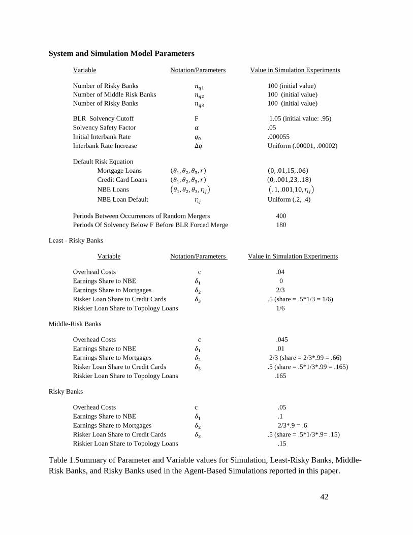
42

System and Simulation Model Parameters

Variable Notation/Parameters Value in Simulation Experiments

Number of Risky Banks 100 (initial value)

Number of Middle Risk Banks 100 (initial value)

Number of Risky Banks 100 (initial value)

BLR Solvency Cutoff F 1.05 (initial value: .95)

Solvency Safety Factor .05

Initial Interbank Rate .000055

Interbank Rate Increase Uniform (.00001, .00002)

Default Risk Equation

Mortgage Loans

Credit Card Loans

NBE Loans

NBE Loan Default Uniform (.2, .4)

Periods Between Occurrences of Random Mergers 400

Periods Of Solvency Below F Before BLR Forced Merge 180

Least - Risky Banks

Variable Notation/Parameters Value in Simulation Experiments

Overhead Costs c .04

Earnings Share to NBE 0

Earnings Share to Mortgages 2/3

Risker Loan Share to Credit Cards .5 (share = .5*1/3 = 1/6)

Riskier Loan Share to Topology Loans 1/6

Middle-Risk Banks

Overhead Costs c .045

Earnings Share to NBE .01

Earnings Share to Mortgages 2/3 (share = 2/3*.99 = .66)

Risker Loan Share to Credit Cards .5 (share = .5*1/3*.99 = .165)

Riskier Loan Share to Topology Loans .165

Risky Banks

Overhead Costs c .05

Earnings Share to NBE .1

Earnings Share to Mortgages 2/3*.9 = .6

Risker Loan Share to Credit Cards .5 (share = .5*1/3*.9= .15)

Riskier Loan Share to Topology Loans .15

Table 1.Summary of Parameter and Variable values for Simulation, Least-Risky Banks, Middle-

Risk Banks, and Risky Banks used in the Agent-Based Simulations reported in this paper.

43

1-Day Payback Period Average Bank Solvency Statistics

Run

All Banks 1 2 3 4 5 6 7 8 9 10

Average 1.1277 1.1266 1.1274 1.1277 1.1271 1.1275 1.1271 1.1271 1.1267 1.1266

Standard Deviation 0.0418 0.0415 0.0419 0.0419 0.0418 0.0417 0.0416 0.0415 0.0413 0.0417

Least Risky Banks

Average 1.0801 1.0788 1.0804 1.0804 1.0797 1.0809 1.0815 1.0810 1.0801 1.0803

Standard Deviation 0.0268 0.0271 0.0274 0.0270 0.0277 0.0269 0.0266 0.0270 0.0275 0.0279

Middle Risk Banks

Average 1.1107 1.1127 1.1106 1.1117 1.1101 1.1104 1.1121 1.1107 1.1113 1.1107

Standard Deviation 0.0377 0.0376 0.0371 0.0380 0.0382 0.0387 0.0377 0.0385 0.0378 0.0376

Risky Banks

Average 1.1860 1.1815 1.1851 1.1865 1.1830 1.1850 1.1865 1.1843 1.1828 1.1825

Standard Deviation 0.0659 0.0647 0.0653 0.0661 0.0644 0.0657 0.0668 0.0648 0.0644 0.0654

Table 2. Solvency statistics for the 10 simulation runs for the 1-day interbank loan payback period case. The simulation run

whose communities are shown in Figures 5, 7 and 9 is highlighted.

3-Day Payback Period Average Bank Solvency Statistics

Run

All Banks 1 2 3 4 5 6 7 8 9 10

Average 1.1269 1.1272 1.1267 1.1276 1.1275 1.1262 1.1277 1.1266 1.1276 1.1268

Standard Deviation 0.0417 0.0419 0.0416 0.0422 0.0419 0.0417 0.0419 0.0416 0.0419 0.0415

Least Risky Banks

Average 1.0803 1.0799 1.0794 1.0799 1.0807 1.0790 1.0809 1.0799 1.0803 1.0811

Standard Deviation 0.0277 0.0280 0.0276 0.0275 0.0274 0.0277 0.0270 0.0278 0.0271 0.0271

Middle Risk Banks

Average 1.1109 1.1112 1.1111 1.1109 1.1105 1.1101 1.1116 1.1121 1.1120 1.1107

Standard Deviation 0.0370 0.0378 0.0373 0.0386 0.0379 0.0376 0.0372 0.0376 0.0371 0.0369

Risky Banks

Average 1.1842 1.1828 1.1831 1.1844 1.1844 1.1813 1.1861 1.1815 1.1849 1.1850

Standard Deviation 0.0663 0.0650 0.0649 0.0660 0.0650 0.0653 0.0664 0.0664 0.0658 0.0664

Table 3. Solvency statistics for the 10 simulation runs for the 1-day interbank loan payback period case. The simulation run whose

communities are shown in Figures 6, 8, and 10 is highlighted.

44

GCAB Regressions Summary Data 1-Day Payback Period

IGB Regressions Summary Data 1-Day Payback Period

Risky

Middle Risk Least Risky

Risky

Middle Risk Least Risky

Run Banks

- Sign %

# Banks

- Sign %

# Banks

- Sign %

# Banks Adj R2

Run Banks

- Sign %

# Banks

- Sign %

# Banks

- Sign %

# Banks Adj R2

1 109 0.1842 38 0.0161 62 0.5556 9 58.90%

1 50 0.1667 18 0 18 0.2143 14 49.60%

2 112 0.1 30 0 74 0.625 8 62.50%

2 48 0.1429 14 0 28 0 6 52.40%

3 116 0.15 40 0.0147 68 0.75 8 56.80%

3 54 0.3077 13 0.0303 33 0.25 8 49.90%

4 101 0.1034 29 0 67 0.4 5 58%

4 54 0.1111 18 0.05 20 0.313 16 50.20%

5 122 0.1860 43 0.0267 75 0.75 4 57.30%

5 50 0.1333 15 0.0370 27 0.125 8 51.40%

6 106 0.1176 34 0 67 0.6 5 57%

6 52 0 15 0 27 0.3 10 50.30%

7 118 0.1316 38 0 72 0.375 8 52.50%

7 52 0.0833 12 0.0714 28 0.3333 12 45.90%

8 111 0.1429 35 0.0147 68 0.625 8 56.70%

8 50 0.1538 13 0.0370 27 0.3 10 51.80%

9 116 0.2051 39 0.0141 71 0.6667 6 55.90%

9 54 0.1667 12 0 31 0.0909 11 49.50%

10 112 0.0789 38 0 70 0.25 4 55.40%

10 53 0 18 0.04 25 0.1 10 48.60%

Table 4. Table 5.

GCAB Regressions Summary Data 3-Day Payback Period

IGB Regressions Summary Data 3-Day Payback Period

Risky

Middle Risk Least Risky

Risky

Middle Risk Least Risky

Run Banks

- Sign

%

#

Banks

- Sign

%

#

Banks

- Sign

%

#

Banks Adj R2

Run Banks

- Sign

%

#

Banks

- Sign

%

#

Banks

- Sign

%

#

Banks Adj R2

1 27 0.6 10 0.167 12 0.2 5 13%

1 22 0.5 10 0.5 6 0.3333 6 10%

2 20 0.444 9 0.429 7 0 4 17.60%

2 18 0.3333 3 0.6 5 0 10 14.60%

3 28 0.429 7 0.143 7 0.286 14 13.90%

3 21 0 4 1 1 0.3125 16 10.70%

4 19 0.667 6 0.333 6 0.286 7 17.20%

4 13 1 1 0.5 4 0.5 8 21.70%

5 36 0.438 16 0.231 13 0 7 21.70%

5 19 0.3333 6 0.625 8 0.2 5 18.60%

6 34 0.5 8 0.111 9 0.412 17 19%

6 24 0.3333 9 0.5 4 0.2727 11 14%

7 29 0.3 10 0.364 11 0.25 8 13.60%

7 22 0 6 0.5 6 0.3 10 10.60%

8 27 0.75 12 0.5 8 0.286 7 16.60%

8 25 0 2 0.5 8 0.4667 15 12.30%

9 13 0.167 6 0.5 4 0.333 3 17.90%

9 23 0.3333 6 0.5 4 0.1538 13 15.60%

10 24 0.5 10 0 8 0.333 6 15.10%

10 17 0.6667 6 0.3333 3 0.125 8 13.10%

Table 6. Table 7.

Tables 4-7. Regression outputs for GCAB regressions for a 1-Day and 3-Day payback periods for interbank loans. The columns

are organized according to whether banks are in the risky, middle-risk, or least-risky category. Data are presented for 10

simulation runs of 3,650 iterations each. The Total Banks column contains the number of banks with significant regression

parameters – parameters for which regression estimates for have p values less than or equal to .05. The – Sign Percent column

indicates the percentage of banks in each category with negative signs on the significant parameter estimate, and the Share of Total

column is the number of significant banks in each category. The Adj R2 category is the adjusted R2 value for the regression

equation.

45

Table 8. Summary results for regressions of number of communities for 10 simulations in each payback

scenario where average system solvency is the dependent variable. The SE rows indicate upper bounds (1-day

payback period) lower bounds (3-day payback period) for the highly-significant parameter estimates in each

case.

Community and Average Solvency Regressions

1-Day Payback Period

Run

1 2 3 4 5 6 7 8 9 10

Communities Parameter -0.00075 -0.00067 -0.00063 -0.00064 -0.0007 -0.00065 -0.00061 -0.00068 -0.00064 -0.00062

Adjusted R(squared) 30.50% 33.80% 35.90% 33.10% 36.30% 31.80% 30.30% 30.10% 34.70% 34.40%

+ 3 SEs -0.0007 -0.00062 -0.00059 -0.00059 -0.00065 -0.0006 -0.00057 -0.00063 -0.0006 -0.00058

+ 2 SEs -0.0006 -0.00061 -0.00058 -0.0006

3-Day Payback Period

Run

1 2 3 4 5 6 7 8 9 10

Communities Parameter -0.00051 -0.00054 -0.00054 -0.00053 -0.00057 -0.0005 -0.00055 -0.00059 -0.00054 -0.00054

Adjusted R(squared) 36.80% 36.70% 35.20% 36% 34.10% 37.60% 35% 34.10% 35.90% 35.20%

- 3 SEs -0.00055 -0.00058 -0.00058 -0.00056 -0.0006 -0.00053 -0.00059 -0.00063 -0.00057 -0.00058

- 2 SEs -0.00061