Solitary Wave Interactions of the Euler{Poisson...

J. math. fluid mech. 5 (2003) 92–1181422-6928/03/010092-27c© 2003 Birkhauser Verlag, Basel

Journal of MathematicalFluid Mechanics

Solitary Wave Interactions of the Euler–Poisson Equations

Mariana Haragus∗, David P. Nicholls† and David H. Sattinger‡

Abstract. We study solitary wave interactions in the Euler–Poisson equations modeling ionacoustic plasmas and their approximation by KdV n-solitons. Numerical experiments are per-formed and solutions compared to appropriately scaled KdV n-solitons. While largely correctqualitatively the soliton solutions did not accurately capture the scattering shifts experienced bythe solitary waves. We propose correcting this discrepancy by carrying out the singular pertur-bation scheme which produces the KdV equation at lowest order to higher order. The foundationfor this program is laid and preliminary results are presented.

Mathematics Subject Classification (2000). 35Q51, 35Q53.

Keywords. KdV equation, plasma equations, resonant soliton interactions.

1. Introduction

Over the past 150 years one of the successes in the application of mathematics toscience and engineering has been in the simulation of nonlinear, dispersive evolu-tionary physical processes by integrable partial differential equations. For example,the Korteweg–de Vries (KdV) and Nonlinear Schrodinger (NLS) equations havebeen used as a models in applications as diverse as ocean wave dynamics, plasmaphysics, and nonlinear optics. Of particular significance in the success of thesemodels is the fact that they are integrable and possess, among other things, soli-ton solutions which propagate without change in form and interact “elastically,”i.e. the waveforms emerge from interactions with the same speed and shape, suf-fering only a scattering shift as evidence of the collision.

A natural question to ask is how well the multi-soliton solutions approximatethe true solutions they are meant to model. In the setting of gravity waves onthe surface of an ideal fluid, modelled by the Euler equations, several answershave been proposed. Craig [3] has shown that suitably scaled solutions of the

∗Research partially supported by the Ministere de la Recherche de la Technologie, ACIjeunes chercheurs.

†Research supported by NSF Grant DMS-0196452.‡Research supported by NSF Grant DMS-9971249.

Vol. 5 (2003) Solitary Wave Interactions of the Euler–Poisson Equations 93

Euler equations are “close” to solutions of the relevant KdV equation for a fi-nite, though potentially quite long, period of time. More recently Schneider &Wayne [12] have shown that suitably scaled and sufficiently small solutions ofthe water wave problem in the long wave limit split up into two wave packets,one moving to the right and one to the left, which evolve independently as so-lutions of two KdV equations on a finite but again potentially quite long timeinterval. Their analysis includes soliton solutions and allows for studying the in-teraction of solitary waves in certain cases. However, the scattering anomaliesin our numerical experiments (see § 3) imply that the scattering shifts experi-enced by the solitary waves are not accurately described by the KdV equationitself.

Zou & Su [13] calculated numerically the second and third order correctionsto the KdV equation for the Euler equations. They found that the interactionis elastic at second order, but that a dispersive tail appears at third order. Fen-ton & Rienecker [5] carried out a numerical study of interacting solitary wavesfor the Euler equations and compared the numerical results with solutions of theKorteweg–de Vries equation. They noted [5]:

Results support . . . applicability of the Korteweg–de Vries equation . . . sincethe waves during interaction are long and low. However, some deviationsfrom the theoretical predictions were observed: the overtaking wave grewsignificantly at the expense of the slower wave, and the predicted phaseshift was only roughly described by the theory.

In fact, the inelastic nature of the interaction has been reported by others studyingsolitary wave interactions for non-integrable dispersive systems [1], [2], [7], [8].

Among the class of nonlinear, dispersive, evolutionary physical models ad-mitting an approximation by the KdV equation, one of the simplest is modelledby the Euler–Poisson equations of ion acoustic plasma physics. These equationsshare many of the same features as the Euler equations which model the evo-lution of the free surface of an ideal fluid such as existence of solitary wavesand a wave of maximum speed, crest instability of solitary waves, Hamiltonianstructure and certain symmetries. However, they lack many of the complicationsof the Euler equations such as the presence of the non-local Dirichlet–Neumannoperator (or one of its analogues) [4] for a formulation which can be naturallyrelated to the KdV equation. While this operator can be analyzed it does ren-der the Euler equations significantly more complicated than the Euler–Poissonequations and for this reason we restrict our current investigations to the latterequation.

A further instance of the inelastic behavior mentioned above, but in the contextof plasma waves, was noticed by Li & Sattinger [9] in a numerical simulation ofinteraction of low amplitude solitary waves (of different amplitude) of the Euler–Poisson equations of plasma physics. They compared their numerically computedsolution with an appropriately scaled 2-soliton solution of the KdV equation andfound a dispersive tail approximately 0.00666% of the magnitude of the smaller

94 M. Haragus, D. P. Nicholls and D. H. Sattinger JMFM

wave, consistent with the dispersive tail at third order found by Zou & Su [13] forwater waves. However, Li & Sattinger’s data did not confirm all of the findingsof Fenton & Rienecker [5] in the case of the water waves. While it did showthat the plasma waves are displaced relative to the KdV waves, the faster wavesdid not gain significant amplitude at the expense of the slower wave. In lightof these findings the authors’ aim in this research project is to understand thediscrepancies between predictions of the KdV n-soliton solution and observationsin numerical simulations on the full Euler–Poisson equations, and to produce, ifpossible, an enhanced model which more accurately captures effects such as thescattering shift.

The message of this paper is two-fold. First, in the setting of the Euler–Poissonequations of plasma physics, the KdV n-soliton solution provides qualitatively ex-cellent results (producing solitary waves which interact essentially elastically evenwell outside of their purported realm of validity) while being quantitatively in-accurate in capturing certain effects (particularly the scattering shift apparentafter a collision). Second, we present some preliminary results on constructing“higher order corrections” to the KdV equation which will accurately capture thequantitative inaccuracies produced by the KdV n-soliton solution.

The paper is organized as follows: Section 2 discusses the Euler–Poisson equa-tions, the derivation of the KdV approximation, the numerical method developedby Li & Sattinger [9], and a convergence study indicating the accuracy, stability,and robustness of the method. In Section 3 we present results of numerical exper-iments on two- and three-pulse interactions in the Euler–Poisson equations andtheir approximation by KdV two- and three-solitons. In Section 4 we discuss someof our preliminary theoretical results. In particular in Section 4.1 we present a dis-cussion of the time-scale of interaction for two solitary waves and in Section 4.2 wediscuss the next-order correction to the KdV equation in a singular perturbationexpansion for the Euler–Poisson equations. Modulational effects on these modelequations during solitary wave interactions, and the relation to the results of Zou& Su [13] are discussed in Section 4.3. Finally, in Appendix A we present someresults on two-soliton solutions of the KdV equation which are used extensively inSection 4.2.

2. Numerical simulation of the Euler–Poisson equations

In this section we present the equations governing the evolution of an ion acousticplasma, i.e. the Euler–Poisson equations (§ 2.1), and present the first step ina singular perturbation expansion of the Euler–Poisson equations which gives theKdV equation at lowest order (§ 2.2). We also briefly describe a numerical methoddue to Li & Sattinger [9] for simulating solutions and present some numericalconvergence studies which give us confidence that our numerical solutions convergeto true solutions of the Euler–Poisson equations (§ 2.3).


2.1. Euler–Poisson equations

The Euler–Poisson equations for ion acoustic waves in plasmas are

nt + (nv)x = 0, vt +(

v2

2+ ϕ

)x

= 0, ϕxx − eϕ + n = 0 (2.1)

where ϕ, n, and v are respectively the electric potential, ion density and ionvelocity. This system supports solitary waves which travel with constant speed[11] (see [9] for a detailed proof of existence). They are solutions of the form(1 + n, v, ϕ)(x − ct), where c is the propagation speed, which decay to zero asξ = (x− ct) → ±∞. Such solutions satisfy the system

n =v

c− v, v = c−

√c2 − 2ϕ, (2.2a)

ϕ′′ = eϕ − c√c2 − 2ϕ

. (2.2b)

Solitary waves exist for supersonic speeds c > 1 and there is a wave of maximumspeed traveling at a rate c ≈ 1.5852. With this quantity one can define a Machnumber by

M(c) =c− 1c− 1

≈ c− 1.5852

, (2.3)

which will appear in several of our numerical experiments.

2.2. KdV approximation

We briefly review the derivation of the KdV equation as the leading term in asingular perturbation scheme for the Euler–Poisson equations. By introducing arescaling of the space and time variables by x′ = εx, t′ = ε3t, where ε is therelevant smallness parameter, one obtains the singular perturbation problem

ε2nt′ + (nv)x′ = 0

ε2vt′ +(

v2

2+ ϕ

)x′

= 0

−ε2ϕx′x′ + eϕ = n.

In the following, we shall drop the primes from the variables. As only even powersof ε appear in these equations, we formally expand all quantities in powers of ε2,

n = 1 + ε2n1 + ε4n2 + . . .

v = −1 + ε2v1 + ε4v2 + . . .

ϕ = ε2ϕ1 + ε4ϕ2 + . . . .

This corresponds to expanding around a density of n = 1 and a velocity at infinityof v = −1, corresponding to a Galilean frame moving with speed 1.


At order ε2 we obtain, by differentiating the third equation with respect to x,

(n1 − v1)x = 0 (v1 − ϕ1)x = 0 (ϕ1 − n1)x = 0. (2.4)

At order ε4 we get

(n2 − v2)x = n1,t + (n1v1)x (2.5a)

(v2 − ϕ2)x = v1,t +12(v2

1)x (2.5b)

(ϕ2 − n2)x = ϕ1,xxx − ϕ1ϕ1,x. (2.5c)

In fact at each step, k, we get a system of equations of the form

(nk − vk)x = f(1)k , (vk − ϕk)x = f

(2)k , (ϕk − nk)x = f

(3)k . (2.6)

The operator on the left side of (2.6) has a null space of the form nk = vk = ϕk,and the solvability condition for the system is

f(1)k + f

(2)k + f

(3)k = 0. (2.7)

The general solution of this system vanishing as x → −∞ is

vk(x, t) = ϕk +∫ x

−∞f

(2)k (x′, t) dx′ (2.8a)

nk(x, t) = ϕk −∫ x

−∞f

(3)k (x′, t) dx′, (2.8b)

where ϕ = ϕ(x, t) is to determined so that the solvability condition at the nextorder is satisfied.

At the lowest order (2.4) & (2.8) require that n1 = v1 = ϕ1, while at next order(2.5) and the solvability condition (2.7) require that ϕ1 satisfy

ut +12uxxx + uux = 0, (2.9)

the KdV equation. The extension of this expansion to next order is the topic of§ 4.2.

Of great significance to the rest of the paper is integrability of (2.9) and theexplicit 2-soliton solution given by

u(x, t) = 6d2

dx2log τ, τ = det

∣∣∣∣∣∣δjk +e−(θj+θk)

ωj + ωk

∣∣∣∣∣∣, (2.10)

whereθj = ωj(x− 2ω2

j t− αj), j = 1, 2. (2.11)

The 2-soliton solution is a four parameter family of solutions of (2.9); the param-eters αj are the relative phases of the two waves and the speeds of the waves aregiven by 2ω2

j . The determinant in (2.10) is called the tau function in the literature.


2.3. Numerical method and convergence

In numerical simulations the spatial boundary condition of decay at infinity isreplaced by the condition that n, v, and ϕ are periodic of period L, where L issuitably large, and the support of these functions is well within the interval [0, L].The numerical method we have utilized for simulations of (2.1) (with the periodicboundary condition previously mentioned) is due to Li & Sattinger and discussedin detail in [9]. To summarize, the method is a Fourier collocation method inspace and an implicit first order finite difference method in time. The spatialdiscretization is chosen for its spectral accuracy while the time stepping strategyis chosen for its simplicity and stability. A raised cosine filter is used periodically(in time) in the spatial variable to counteract the effects of aliasing errors.

In order to build confidence in the reliability of our scheme we performed anumerical convergence study on the problem of two solitary plasma waves collidingat relatively low Mach number. In particular, we simulated the evolution of twosuperposed solitary wave solutions of (2.1) with speeds c1 = 1.1 and c2 = 1.3 onan interval of length L = 100 for a time interval of length T = 490. Equations(2.1) were solved with c = 1.2 so that the solutions simply exchanged positions,and discretizations were made in space and time parameterized by the number ofcollocation points Nx and the number of time steps Nt. To help control aliasingerrors, the raised cosine filter was applied after every 100 units of time.

The results of this study for fixed Nt = 49000 (∆t = 0.01) and varying Nx aregiven in Table 1 where the “exact solution” is given by the results of a simulationwith Nx = 16, 384 (∆x = 0.006103515625). The results for varying Nt and fixed

Nx ∆x Error in ϕ (Discrete L2)

256 0.390625 0.01146778606810997512 0.1953125 0.0028703032778815011024 0.09765625 3.427685711428991e× 10−5

2048 0.048828125 1.715995772970149× 10−7

4096 0.0244140625 8.53361553374557× 10−9

8192 0.01220703125 5.299269878231338× 10−9

Table 1. Convergence study of two solitary wave interaction at speeds c1 = 1.1 and c2 = 1.3with fixed Nt = 49000 (∆t = 0.01) and variable Nx.

Nx = 1024 (∆x = 0.09765625) are given in Table 2, where the “exact solution”is given by the approximation with Nt = 196, 000 (∆t = 0.0025). In each casewe see clearly that as the discretization is increased the approximate solution isconverging to the “exact solution.” Furthermore, as Nx is increased the rate ofconvergence is spectral, as one would expect from a Fourier collocation method ona periodic interval, and as Nt is increased the rate of convergence is roughly linearas expected from a first order scheme.


Nt ∆t Error in ϕ (Discrete L2)

6,125 0.08 0.149393126632467412,250 0.04 0.120084795335007924,500 0.02 0.0750657384475513549,000 0.01 0.0364502509874921798,000 0.005 0.01266804809229405

Table 2. Convergence study of two solitary wave interaction at speeds c1 = 1.1 and c2 = 1.3with fixed Nx = 1024 (∆x = 0.09765625) and variable Nt.

3. Numerical results

We conducted several numerical experiments regarding the interaction of solitarywave solutions of the Euler–Poisson equations (2.1) in order to gain some insightinto the strengths and weaknesses of the KdV approximation to these equations.In all experiments the individual traveling waves were constructed by a numericalcontinuation method applied to (2.1) for steady solutions, i.e. nt = vt = ϕt = 0,where the parameter was the speed c and an initial guess of a properly scaled KdVsoliton was used to step off the trivial branch of solutions (n = v = ϕ ≡ 0). Tosimulate two or more solitary waves interacting, two or more of these solutions weresimply added together and, provided that the pulses were sufficiently separatedin space, our results were excellent. In the experiments below, the relationshipbetween the absolute wave speed cj of pulse j in the rest frame to the solitarywave speed parameter ωj is cj = 1 + 2ω2

j .In the first experiment we compared a high Mach number (M = 0.8544) solitary

wave solution of the Euler–Poisson equation with a KdV soliton moving with thesame speed. In Figure 1 we see the results of this computation and notice that theplasma wave (dashed line) is considerably more peaked than the KdV wave of equalvelocity (solid line). The KdV solitary wave is 6ω2sech2ωx, where c = 1 + 2ω2.

In the next two experiments we study two- and three-pulse interactions in theEuler–Poisson equations and compare them with two- and three-soliton solutionsof KdV with speeds that match those of the plasma pulses. In Figures 2 & 3 wesee the results after matching KdV two- and three-solitons, respectively, to theinitial data of the plasma using the initial location of the wave peaks and theinitial speeds. The experiments clearly confirm the displacement of the plasmawaves relative to the corresponding KdV waves after the interaction, as noted byFenton & Rienecker [5] in the context of water waves.

Note that in Figure 2 the smaller plasma wave is completely absorbed by thelarger one in the course of the interaction, while in the interaction between wavesof speeds 1.05 and 1.1, depicted in the sequence in Figure 4 from Li & Sattinger [9],momentum is exchanged between the faster and slower waves. This phenomenon iswell known for the 2-soliton solutions of the KdV equation: when the wave speedsare close, there is a momentum transfer, while in the case of a large differencebetween the wave speeds, the slower wave is overtaken and absorbed by the fasterwave.


0 5 10 15 20 250

0.2

0.4

0.6

0.8

1

1.2

1.4

1.6

c=1.5, M=.8544

KdV approximation at high mach number

KdV: dashed line

Fig. 1. Comparison of the KdV soliton (dashed) with the ϕ wave (solid) of the ion acousticplasma equations at M = .8544, c = 1.5.

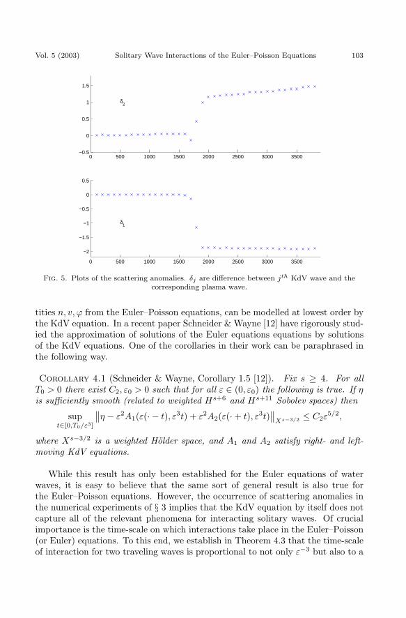
The concept of scattering shift for the KdV equation is based on the fact thatthe emerging waves travel at the same speeds as the incoming waves, and the waveslose no energy in the course of the interaction. The trailing dispersive waves ofvery low magnitude found in the numerical experiments of Li & Sattinger [9] andpredicted by Zou & Su [13] imply that energy is lost from the traveling wavesin the course of the interaction, so that the total energy of the emerging wavesis slightly less than that of the incoming waves. If this were the case, then theemerging waves would travel at slightly different speeds than the incoming solitarywaves, and the distance between the plasma wave and the corresponding KdV waveafter the interaction would grow linearly in time, as indicated by the plots of thescattering anomalies in Figure 5. In this plot, the δj are difference between jth

KdV wave and the corresponding plasma wave. The anomalies develop on a fasttime scale at the time of the interaction. For large times, δ2 appears to increaselinearly, suggesting that the faster plasma wave falls away from the KdV wave ata constant speed; while the decay in δ1 suggests that the slower plasma wave hasgained speed.

If the waves are asymptotic to solitary waves after they emerge from the in-teraction, then Figure 5 suggests that the faster plasma wave loses speed in theinteraction, while the slower plasma wave picks up speed in the interaction. Thus,there is a small momentum transfer from the faster to the slower wave duringthe interaction. In addition, the presence of a trailing dispersive wave indicates


0 5 10 15 20 25 30 35 40 45 500

0.5

1

1.5

t=0

0 5 10 15 20 25 30 35 40 45 500

0.5

1

1.5

t=62.5

0 5 10 15 20 25 30 35 40 45 500

0.5

1

1.5

t=125

Fig. 2. Comparison of the KdV 2-soliton solution (dashed) with the ϕ wave (solid) of the ionacoustic plasma equations at initial, intermediate, and final configurations. (c1 = 1.1, c2 = 1.5)

that some energy is lost from the waves in the course of the interaction. Table 3gives the numerical values of the speeds of the waves, measured from the data; inthis table cj is the speed of each individual pulse computed as a solitary wave, v0

and A0 are the initial (pre-collision) speed and amplitude, while vf and Af arethe final (post-collision) speed and amplitude. The data show that the emitted

Run cj v0 A0 vf Af

1 1.05 1.0501 .1446 1.0499 .14471.10 1.0999 .2795 1.0999 .2789

2 1.1 1.0999 .2795 1.1003 .27901.3 1.2997 .7422 1.2964 .7341

3 1.1 1.1000 .2795 1.100 0.27971.4 1.3996 .9383 1.3939 0.9271

4 1.1 1.0998 .2795 1.1003 0.27901.5 1.5000 1.1165 1.4987 1.1144

Table 3. Numerical experiments on interacting two-pulse solutions of the Euler–Poissonequations: cj are the theoretical solitary wave speeds; v0 and vf their observed speeds before

and after the interaction; A0 and Af their observed amplitudes before and after the interaction.

waves are very close in speed to the initial waves, while the plots of the scatteringanomalies indicate that the faster wave loses speed during the interaction. Themost significant qualitative difference between the KdV approximation and thesolutions of the Euler–Poisson equations themselves lies in the displacement of the


0 10 20 30 40 50 60 70 800

0.5

1

1.5

0 10 20 30 40 50 60 70 800

0.5

1

1.5

0 10 20 30 40 50 60 70 800

0.5

1

1.5

Fig. 3. Comparison of the KdV 3-soliton solution (dashed) with the ϕ wave (solid) of the ionacoustic plasma equations at initial, intermediate, and final configurations.

(c1 = 1.3, c2 = 1.4, c3 = 1.5)

emerging waves from those of the 2-soliton solution of the KdV equation.In a completely elastic interaction the waves retain their original shape, speed,

and amplitude. Thus a rough measure of the elasticity of the interaction can beobtained by translating one of the waves, say the faster one, back to its originalposition and comparing it with the corresponding wave prior to the interaction. Inthe experiment discussed in Li & Sattinger [9] there was no difference graphicallywhen this was done with the larger wave. A quantitative measure of the elasticityof the interaction can be obtained by defining a coefficient of elasticity of theinteraction, as follows:

e = 1− ||v0 − vft||1||v0||1 , ||v||21 =

∫v2

x + v2 dx.

Here, v0 is the initial wave form, while vft is the final waveform, translated backto its original position. By this measure the solitary wave interactions for theEuler–Poisson equations are highly elastic, even at high Mach numbers, in thesense that the faster wave regains its initial shape after the interaction, as shownin Table 4. The experimental runs in Table 4 are the same as those in Table 3.


60 70 80 90 100 110 120 130 140 1500

0.1

0.2

0.3

t=800

60 70 80 90 100 110 120 130 140 1500

0.1

0.2

0.3

t=1600

60 70 80 90 100 110 120 130 140 1500

0.1

0.2

0.3

t=2000

60 70 80 90 100 110 120 130 140 1500

0.1

0.2

0.3

t=2600

Fig. 4. Comparison of the KdV 2-soliton solution (dashed) with the ϕ wave (solid) of the ionacoustic plasma equations at initial, two intermediate, and final configurations [9].

(c1 = 1.05, c2 = 1.1)

Run M1 M2 e ∆x

1 0.0854 0.1709 0.9862 0.02452 0.1709 0.5126 0.9647 0.01223 0.1709 0.6835 0.9664 0.00374 0.1709 0.8544 0.9739 0.0031

Table 4. Elasticity coefficients e of interacting two-pulse solutions of the Euler–Poissonequations with Mach numbers M1 and M2 (cf. Table 3); ∆x is the grid spacing.

4. Preliminary theoretical results

It is evident from the numerical experiments of § 3 that the KdV approxima-tion of the Euler–Poisson equations (2.9) cannot provide complete details aboutsolitary wave interactions alone. In this section we present our preliminary re-sults regarding efforts in this direction, particularly commenting on the results ofSchneider & Wayne [12] and Zou & Su [13], and our own progress on carrying outthe perturbation expansion begun in Section 2.2 to higher order.

4.1. Time-scale of solitary wave interactions

In Eulerian variables, the Euler equations of water waves have a quantity η(x, t),the elevation of the free surface from the undisturbed state, which, like the quan-


0 500 1000 1500 2000 2500 3000 3500−0.5

0

0.5

1

1.5

δ2

0 500 1000 1500 2000 2500 3000 3500

−2

−1.5

−1

−0.5

0

0.5

δ1

Fig. 5. Plots of the scattering anomalies. δj are difference between jth KdV wave and thecorresponding plasma wave.

tities n, v, ϕ from the Euler–Poisson equations, can be modelled at lowest order bythe KdV equation. In a recent paper Schneider & Wayne [12] have rigorously stud-ied the approximation of solutions of the Euler equations equations by solutionsof the KdV equations. One of the corollaries in their work can be paraphrased inthe following way.

Corollary 4.1 (Schneider & Wayne, Corollary 1.5 [12]). Fix s ≥ 4. For allT0 > 0 there exist C2, ε0 > 0 such that for all ε ∈ (0, ε0) the following is true. If ηis sufficiently smooth (related to weighted Hs+6 and Hs+11 Sobolev spaces) then

supt∈[0,T0/ε3]

∥∥η − ε2A1(ε(· − t), ε3t) + ε2A2(ε(·+ t), ε3t)∥∥

Xs−3/2 ≤ C2ε5/2,

where Xs−3/2 is a weighted Holder space, and A1 and A2 satisfy right- and left-moving KdV equations.

While this result has only been established for the Euler equations of waterwaves, it is easy to believe that the same sort of general result is also true forthe Euler–Poisson equations. However, the occurrence of scattering anomalies inthe numerical experiments of § 3 implies that the KdV equation by itself does notcapture all of the relevant phenomena for interacting solitary waves. Of crucialimportance is the time-scale on which interactions take place in the Euler–Poisson(or Euler) equations. To this end, we establish in Theorem 4.3 that the time-scaleof interaction for two traveling waves is proportional to not only ε−3 but also to a


second parameter, the difference between the speeds of the two interacting waves.Independent of the size of ε, by making the speeds of the interacting waves close,one can make the time of interaction arbitrarily large, possibly larger than thetime-scale covered by Schneider & Wayne.

The problem we consider is somewhat ambiguous, since solitary waves are notcompactly supported, thus the waves never separate completely. To make thediscussion concrete, we make the following definition:

Definition 4.2. Two solitary waves are separated to threshold r% (0 < r < 100)if the solution contains two distinct pulses, and, somewhere, denoted αr, betweenthe maxima of these two pulses the magnitude of the solution is (r/100)A whereA is the L∞ norm of the solution.

In light of Definition 4.2 we are able to establish the following theorem.

Theorem 4.3. The time required for two solitary waves of the KdV equation tocompletely interact, given a threshold of r%, is given by

T =αr

ω1ω2(ω2 − ω1)− 1

2ω1ω2(ω2 + ω1)log

[ω2 + ω1

ω2 − ω1

], (4.1)

where sech2αr = 0.01r.

Proof. The exact formula for the length of time required for the interaction oftwo solitary waves of the KdV equation is obtained by first calculating the timerequired for two free waves to interact, and then correcting for the scattering shift.

The relative velocity of two free waves with speeds 2ω2j , is 2(ω2

2 − ω21). The

relative distance traveled by the overtaking wave during the course of the inter-action is the sum of the widths of the two waves. If l denotes the width of thesolitary wave of speed 2ω2, and we use r% as the threshold, we get ωl/2 = αr,where sech2 αr = .01r. The total relative distance the faster wave must travel tocompletely overtake and pass the slower wave is therefore

d = l1 + l2 = 2αr

(1ω1

+1ω2

).

The time required for the interaction of two free waves is

2αr

(1ω2

+1ω1

)2(ω2

2 − ω21)

=αr

ω1ω2(ω2 − ω1).

During the interaction, the faster wave is shifted forward, and the slower wave isshifted backward, by the amounts

1ω2

logω2 + ω1

ω2 − ω1,

1ω1

logω2 + ω1

ω2 − ω1,


respectively. The boost due to the scattering of the waves effectively reduces thenet distance the interacting waves must travel by(

1ω2− 1

ω1

)log

ω2 + ω1

ω2 − ω1.

Dividing this expression by the relative velocity and simplifying, we obtain thesecond term in (4.1).

According to Schneider & Wayne [12], solutions of the Euler equations, andpresumably the Euler–Poisson equations, are close to the scaled 2-soliton solutionε2u(εx, ε3t), u being the 2-soliton solution of KdV, on a time scale of order ε−3. Inthis scaling the speeds ω1 and ω2 of the KdV solitons scale as εω1 and εω2, and theinteraction time T in (4.1) therefore scales as ε−3. This shows that the time scaleof the interaction is the same as that for the validity of the KdV approximation.However, Eqn. (4.1) further shows that the interaction time goes to infinity asω1 → ω2, as one would expect. Thus the time required for the complete interactionof two solitary waves depends not only on the small parameter the theory, ε, butalso on a second parameter δ = ω1 − ω2. Therefore one cannot assert, withoutfurther analysis, that the result obtained in [12] is always sufficient to see theinteraction of two solitary waves for sufficiently small ε.

4.2. The perturbation scheme

As we have seen in § 2.2 the KdV equation is the leading term in a singularperturbation scheme for the Euler–Poisson equations. In this section we derive amethod for obtaining a next-order correction to the KdV equation, and obtain ananalytical expression for the second order term to the 2-soliton solution.

Recall from § 2.2 that at each order, k, in the perturbation expansion forapproximating the Euler–Poisson equations we are required to solve a system ofequations (2.6) of the form

(nk − vk)x = f(1)k , (vk − ϕk)x = f

(2)k , (ϕk − nk)x = f

(3)k , (4.2)

where the solvability condition (2.7) is given by f(1)k + f

(2)k + f

(3)k = 0 and the

general solutions for nk and vk in terms of ϕk are given by (2.8). The solvabilitycondition at order four gives the KdV equation (2.9) for ϕ1.

At order ε6 we have

(n3 − v3)x = n2,t + (n1v2 + n2v1)x (4.3a)(v3 − ϕ3)x = v2,t + (v1v2)x (4.3b)

(ϕ3 − n3)x = ϕ2,xxx − (ϕ1ϕ2)x − 16(ϕ3

1)x. (4.3c)

The solvability condition at this order is obtained by setting the sum of the right


hand sides equal to zero, as before. This leads to

Lϕ2 = DF(ϕ1), (4.4)

where L is the linearized KdV operator at ϕ1

Lw = wt +12wxxx + (ϕ1w)x

and

DF(ϕ1) =54ϕ1ϕ1,xxx +

12(ϕ2

1,x)x +34ϕ1,xxt

=∂

∂x

[54ϕ1ϕ1,xx − 1

8ϕ2

1,x −38(ϕ1,xx + ϕ2

1)xx

]

=∂

∂x

[12ϕ1ϕ1,xx − 7

8ϕ2

1,x −38ϕ1,xxxx

].

Thus,

F(ϕ1) =12ϕ1ϕ1,xx − 7

8ϕ2

1,x −38ϕ1,xxxx. (4.5)

Using the analytical results derived in Appendix A we solve this equation explic-itly when ϕ1 is a 2-soliton solution of KdV (similar results hold for the n-solitonsbut we do not consider them here). From (A.14b) and (A.13) we find

F(ϕ1) =74ϕ1ϕ1,xx − 1

4ϕ2

1,x +512

ϕ31 − 72

2∑j=1

ω5j Fj , (4.6)

where Fj is a squared eigenfunction of the Schrodinger operator associated withthe KdV equation (see Appendix A). The derivative of the first three terms in(4.6) is

74ϕ1ϕ1,xxx +

58

(ϕ2

1,x

)x

+54ϕ2

1ϕ1,x. (4.7)

From (A.13) with j = 2 and (A.14a) we get the identity

ϕ1ϕ1,xxx = 48ϕ1(ω31DF1 + ω3

2DF2)− 2ϕ21ϕ1,x, (4.8)

and the three terms in (4.7) reduce to

94ϕ2

1ϕ1,x +54ϕ1,xϕ1,xx + 84ϕ1(ω3

1DF1 + ω32DF2) (4.9)

Putting all these identities together, we see that the right hand side h = DF(ϕ1)of (4.4) can be written as

h =54ϕ1,xϕ1,xx − 9

4ϕ2

1ϕ1,x +2∑

j=1

(84ω3

j ϕ1 − 72ω5j

)DFj . (4.10)


Using (A.22), (A.23), (A.21), and (A.24) we find, after some computations (cf.also [13]), that the second order correction to the 2-soliton solution is

ϕ2 = −94ϕ2

1 − 4ϕ1,xx +2∑

j=1

(84ω3

j Ej − 72ω5j tDFj

), (4.11)

where

Ej = ω1

(∂F1

∂ωj

)θj

+ ω2

(∂F2

∂ωj

)θj

.

To this particular solution we may add any linear combination of homogeneoussolutions of the linearized KdV equation:

2∑j=1

∂ϕ1

∂αj∆αj +

∂ϕ1

∂ωj∆ωj , (4.12)

(see Theorem A.3). Presumably, the coefficients ∆αj and ∆ωj are uniquely deter-mined at the next order of the perturbation scheme by making the equations atnext order solvable; but the computations at third order are quite complicated.

The secular terms tDFj in (4.11) are resonance terms due to the appearanceof DFj in the right side of (4.4). These terms can be eliminated by modulatingthe 2-soliton solution; this will be discussed in § 4.3. Notice that in the secondorder correction to the 1-soliton solution these secular terms can be eliminatedby restricting to traveling waves. The second order approximation to the solitarywave is

Σ = Σ1 + Σ2, (4.13)

where Σ1 is the KdV solitary wave

Σ1(θ) = 6ω2sech2(θ), θ = ω(x− 2ω2t− α),

and Σ2 is a solution of (4.4) for ϕ1(x, t) = Σ1. In this case a solution can be foundby transforming to a moving coordinate system; then (4.4) reduces to a third orderordinary differential equation. Integrating once, we obtain

Σ′′2 + (12sech2 θ − 4)Σ2 = 9ω4(36 sech4θ − 4 sech2 θ − 43 sech6θ

). (4.14)

The explicit solution to this equation was obtained by the method of variation ofparameters, with assistance from Maple,

Σ2(θ) =94ω4 [20− 23 cosh 2θ + 4θ sinh 2θ] sech4(θ). (4.15)

We see that there are no secular terms when only one solitary wave is present, andit is not necessary to introduce an amplitude wave speed correction, as in [13].The first and second order approximations are depicted in Figure 6.


30 35 40 45 50 55 60 65 700

0.05

0.1

0.15

0.2

0.25

0.3

30 35 40 45 50 55 60 65 700

0.05

0.1

0.15

0.2

0.25

0.3

Fig. 6. Upper: The solitary ϕ-wave solution of the ion acoustic plasma equation (solid) andthe KdV solitary wave (dashed). Lower: ϕ wave (solid) vs. the second KdV approximation

(dashed). The wave speed is c = 1.1, ω = 0.2231.

4.3. Modulation and resonant interactions

We saw in the last section that the second order term, given by (4.11), has secularterms which grow in time for interacting solitary waves. These terms must beeliminated in order to get a uniform approximation at second order. In this sectionwe formally set ε = 1 and use instead ω1 and ω2 as small parameters in the theory.For example, the solitary wave 6ω2sech2θ is second order in ω. By Theorem A.7the 2-soliton solution ϕ1 is second order in ω1 and ω2. Since ω1 < ω2 we use ω2

as a measure of relative size of terms in the expansion.Returning to the formal expansion of § 4.2, we write the first two terms as

ϕ = ϕ1 + ϕ2, where L(ϕ2) = DF(ϕ1). By Theorem A.3

∂ϕ1

∂αj= −12ωjDFj .

Hence by (4.11) and (4.12)

ϕ2 = ϕ2 + N2, (4.16)


where

N2 =2∑

j=1

∂ϕ1

∂αj(∆αj + 6ω4

j t) +∂ϕ1

∂ωj(∆ωj)

and

ϕ2 = −94ϕ2

1 − 4ϕ1,xx + 842∑

j=1

ω3j Ej .

Lemma 4.4. For fixed λ = ω1/ω2, ϕ2 is O(ω42), uniformly in x and t. In order

that N2 be O(ω42) it is sufficient that

∆αj = O(ωj), ∆ωj = O(ω2j ), |t| = O(ω−3

2 ),

and that|x− 6ω2

j t− αj | = O(1).

Proof. By Theorem A.7, ϕ1 is O(ω22) and differentiation with respect to x is O(ω2).

It follows that ϕ21 and ϕ1,xx are O(ω4

2). Again by Theorem A.7, Ej is uniformlyO(ω2) hence the terms ω3

j Ej are O(ω42), uniformly in x and t.

We have∂ϕ1

∂αj=

∂ϕ1

∂θj

∂θj

∂αj= −ωj

∂ϕ1

∂θj,

∂ϕ1

∂ωj=

∂ϕ1

∂θj

∂θj

∂ωj=

∂ϕ1

∂θj(x− 6ω2

j t− αj).

Since derivatives with respect to θj are order 1, and ϕ1 is order ω22 , the statements

concerning the order of N2 follow.

When the conditions of Lemma 4.4 are satisfied, the second order approxima-tion can be written

ϕ = ϕ1 + (ϕ2 + N2) = (ϕ1 + N2) + ϕ2.

Let ϕ1 = ϕ1(θ1, θ2, ω1, ω2), where

ωj = ωj + ∆ωj , αj = αj + ∆αj + 6ω4j t,

andθj = ωj(x− 2ω2

j t− αj) = ωj(x− (2ω2j + 6ω4

j )t− αj −∆αj).

Thenϕ1 = ϕ1 + N2 + O(ω6

2),

where ϕ1 is the modulated 2-soliton solution and ϕ1 = ϕ1(θ1, θ2, ω1, ω2) is theoriginal 2-soliton solution.


Theorem 4.5. When the conditions of Lemma 4.4 are satisfied, the formal ap-proximation to the ϕ wave of the plasma equations is given to second order byϕ = ϕ1 + ϕ2.

There are three time regimes in the 2-soliton interaction, which must be treatedseparately. In the first and last, the two solitons are separated and do not interact.Thus, ϕ1 may be approximated by the sum of the two solitary waves. In this case,the second order correction is given by sums of solitary waves and their secondorder corrections (4.15). Prior to the interaction the initial wave speeds are givenby 2ω2

j . After the interaction, the phases and speeds are somewhat different dueto the interaction.

In the vicinity of the interaction, we use the modulated two-soliton interactionϕ of Theorem 4.5 constructed above. A solution of this type was proposed inZou & Su [13] for the entire interaction, −∞ < t < ∞, but this approximationis not justified for all time, since the conditions of Lemma 4.4 are met only overtime intervals of order O(ω−3

2 ). For the experiment in [9], ω2 = .2231 and ω−32 ≈

90, whereas the two solitary waves are found to overlap during the time interval1500 ≤ t ≤ 2300. The terms ∂ϕ1/∂ωj in the nullspace of L were not included in thesecond order approximation in Zou & Su [13]. On the other hand, Figure 2 showsthat the faster plasma wave drops behind the KdV wave during the interaction,hence we must have

2ω22 + 6ω4

2 < 2ω22 .

This implies that ω2 < ω2, and hence ∆ω2 < 0, and some correction to the ωj isnecessary. The theoretical values of ∆ωj and ∆αj cannot be obtained by consid-ering second order terms alone. They presumably are determined by casting outresonances at third order, but the computations at third order are too complicatedto be obtained analytically [13].

A. Theoretical results regarding KdV 2-solitons

A.1. Eigenfunctions of the Schrodinger operator

The KdV equation which occurs in the approximation of the Euler–Poisson equa-tions takes the form (cf. (2.9))

ut +12uxxx + uux = 0. (A.1)

Equation (A.1) can be written in the operator form L = [B,L], where

L = D2 +u

3, B = −2D3 − 1

2(uD + Du).

The wave functions satisfy the pair of equations

Lψ + k2ψ = 0, ψt −Bψ = 0, (A.2)


and (A.1) is the compatibility condition for this over-determined system. Wedenote by ϕ+(x, t, k) and ψ+(x, t, k) the solutions of (A.2) with the asymptoticbehaviors

ϕ+(x, t, k) ∼e−ik(x−2k2t), x → −∞,

ψ+(x, t, k) ∼eik(x−2k2t), x →∞.

The wave function ψ+ tends to zero exponentially as x →∞ for Im(k) > 0; whileϕ+ tends to zero exponentially as x → −∞ for Im(k) > 0. The eigenvalues of theSchrodinger equation Lψ + k2ψ = 0 are those values k = iωj (ωj > 0) for whichϕ+(x, t, iωj) = cjψ+(x, t, iωj) for some constant cj , called the coupling coefficient.The parameters ωj are precisely those which appear in (2.11). We denote thecorresponding eigenfunctions, which decay exponentially as x → ±∞, by ψj .

The eigenfunctions ψj can be obtained by solving a linear system of algebraicequations, which are obtained as a finite dimensional reduction of the Gel’fand–Levitan integral equation for inverse scattering [6]. For the 2-soliton solution theeigenfunctions are obtained in closed form, as follows. Let

Djk = δjk +e−(θj+θk)

ωj + ωk, E =

(e−θ1

e−θ2

).

By Cramer’s rule

ψk = −Dk

τ,

where τ = τ(x, t) is the determinant of the matrix D = ||Djk||, and Dk is thedeterminant of the matrix obtained by replacing the kth column of D by E, k =1, 2.

The two wave functions are given by

D1 = e−θ1 − e−(θ1+2θ2)ω2 − ω1

2ω2(ω2 + ω1)= 2e−(θ1+θ2+β2) sinh (θ2 + β2), (A.3)

D2 = e−θ2 + e−2θ1−θ2ω2 − ω1

2ω1(ω2 + ω1)= 2e−(θ1+θ2+β1) cosh (θ1 + β1), (A.4)

where

βj = −12

logω2 − ω1

2ωj(ω2 + ω1);

and

τ = 1 +e−2θ1

2ω1+

e−2θ2

2ω2+

e−2(θ1+θ2)

4ω1ω2

(ω1 − ω2

ω1 + ω2

)2

. (A.5)

Thus

ψ1 = −2e−β2 sinh(θ2 + β2)κ

, ψ2 = −2e−β1 cosh(θ1 + β1)κ

, (A.6)


where

κ = eθ1+θ2τ = eθ1+θ2 +e−(θ1+θ2)

4ω1ω2

(ω1 − ω2

ω1 + ω2

)2

+eθ2−θ1

2ω1+

eθ1−θ2

2ω2. (A.7)

For k = iωj there is a second solution ϕj of the equations (A.2) which growsexponentially as x → ±∞. (Since the potential u decays exponentially as x →±∞, there is only one exponentially decaying solution. The second solution growsexponentially.)

Lemma A.1. The second solution ϕj of the Schrodinger equation in (A.2) can beobtained as

ϕj =∂

∂k(ϕ+ − cjψ+)

∣∣∣k=iωj

, (A.8)

where cj is the coupling coefficient. The solution ϕj grows linearly in x and t.

Proof. The linear growth of ϕj in x and t is due to the differentiation of thewave functions ϕ+(x, t, k) and ψ+(x, t, k) with respect to the spectral parameterk. Hence Gj contains secular terms which grow linearly in x and t.

Differentiating the first equation in (A.2) with respect to k, we find that thepartial derivatives of ϕ+ and ψ+ with respect to the spectral parameter k satisfy

(L + k2)∂ϕ+

∂k+ 2kϕ+ = 0, (L + k2)

∂ψ+

∂k+ 2kψ+ = 0.

Now set k = iωj in each of these equations, multiply the second equation by cj

and subtract it from the first equation. Since ϕ+(x, t, iωj) = cjψ+(x, t, iωj), wefind that Lϕj − ω2

j ϕj = 0, where ϕj is given in (A.8).Since the two soliton solution u decays exponentially as x → ±∞, only one so-

lution of (A.2) decays exponentially at both ±∞. Since ϕj is linearly independentof ψj , it necessarily grows exponentially.

Remark A.2. The coupling coefficients are given by:

cj =12e2ωjαj

ω1 − ω2

ωj(ω1 + ω2).

A.2. Solutions of the linearized KdV equation

The pair of functions Fj = ψ2j , Gj = ψjϕj , called the squared eigenfunctions,

satisfy the equations

[D3 +23(uD + Du·)− 4ω2

j D]Fj = 0, (A.9)

∂

∂tFj +

12D3Fj + uDFj = 0, (A.10)


where u is the corresponding solution of the KdV equation [6]. Equation (A.10)is called the associated linear equation. Differentiating (A.10) with respect to x,we find that DFj and DGj satisfy the linearized KdV equation

LDFj = LDGj = 0, (A.11)

whereLw = wt +

12wxxx + (uw)x (A.12)

is the KdV operator, linearized at u.The derivatives of the 2-soliton solution with respect to the four parameters

α1, α2, ω1, ω2 are also solutions of (A.12). This follows by differentiating the KdVequation itself for the 2-soliton solution with respect to each of these four param-eters. The relation between these two sets of solutions is given in the followingtheorem.

Theorem A.3. The sets{∂u

∂α1,

∂u

∂α2,

∂u

∂ω1,

∂u

∂ω2

},

{DF1, DF2, DG1, DG2

},

are both solutions of the linearized KdV equation. The relationship between themis given by

∂u

∂aj=

4∑k=1

HjkDFk,

where F3 = G1, F4 = G2, a = (α1, α2, ω1, ω2), and

Hjk =− 12ωje2ωjαj δjk, j = 1, 2, 1 ≤ k ≤ 4;

Hjk =24(

ω1 + ω2

ω1 − ω2

)2

ω2j−2e

−2ωj−2αj−2δjk, j, k = 3, 4;

H31 =6e2ω1α1

ω1(ω22 − ω2

1)

[(2α1ω1 − 1)(ω2

1 − ω22) + 2ω1ω2

];

H42 =6e2ω2α2

ω2(ω21 − ω2

2)

[(2α2ω2 − 1)(ω2

2 − ω21) + 2ω1ω2

];

H32 =12ω2e

2ω2α2

ω22 − ω2

1

, H41 =12ω1e

2ω1α1

ω21 − ω2

2

.

Proof. These relations were determined by extensive computations using the soft-ware package Maple. One may simplify the relationships by setting the phaseconstants α1 = α2 = 0.


A.3. Identities

The KdV equation has also the structure of an infinite dimensional Hamiltoniansystem, and can be written in the form

ut =d

dx

δH2

δu, H2(u) =

∫ ∞

−∞

u2x

4− u3

6dx,

the functional H2 being the Hamiltonian for the system. There are, moreover,an infinite number of Hamiltonians in involution with H2 with respect to theGardner–Poisson bracket, [10].

When the solution of the KdV equation is a multi-soliton, the gradients of thishierarchy of Hamiltonians are linear combinations of the squared eigenfunctions[6]. (In Theorem 3.5 of [6] the An in are obtained as solutions the Lenard recursionrelation, equation (3.20) in that article, but these are the gradients of the densities,not the densities themselves, as stated in the article.) With the present scaling,

δHj

δu= (−2)j−112

2∑k=1

ω2j−1k Fk. (A.13)

Remark A.4. The normalization of the squared eigenfunctions in (A.13) is thatobtained by solving the linear system of algebraic equations which comes from theGel’fand–Levitan equation of inverse scattering [6].

The gradients of the first three conservation laws are:

δH1

δu= u,

δH2

δu= −1

2(uxx + u2), (A.14a)

δH3

δu=

14uxxxx +

56uuxx +

512

u2x +

518

u3. (A.14b)

In particular, taking j = 1 in (A.13), we obtain a representation of the 2-solitonsolution itself as a sum of the squared eigenfunctions:

u = 122∑

k=1

ωkFk. (A.15)

We derive a number of identities which are used in the perturbation theory of§ 4.2. Since uDFj = D(uFj)− FjDu, it follows from (A.15) that

LFj = FjDu, LGj = GjDu. (A.16)

By a direct computation, using (A.9), (A.10), (A.12), and (A.16), we find

L[D

((x− 6ω2

j t)Fj

)]= L[

(x− 6ω2j t)DFj + Fj

]= −uDFj . (A.17)


By (A.15) we find, for αj = 0,

∂u

∂ωj=12Fj + 12

(ω1

∂F1

∂θj+ ω2

∂F2

∂θj

)(x− 6ω2

j t) + 12Ej

=12[Fj +

112

(x− 6ω2j t)

∂u

∂θj+ Ej

], (A.18)

where

Ej = ω1

(∂F1

∂ωj

)θj

+ ω2

(∂F2

∂ωj

)θj

. (A.19)

Here ( )θjdenotes partial differentiation with θj held constant.

Lemma A.5. We have∂u

∂θj= 12DFj ,

where u, the 2-soliton solution, is regarded as a function of θj , ωj.

Proof. By Theorem A.3,∂u

∂αj= −12ωjDFj ,

at αj = 0. On the other hand,

∂u

∂αj=

∂u

∂θj

∂θj

∂αj= −ωj

∂u

∂θj,

and the result follows.

As a consequence of Lemma A.5, (A.18) can be written

∂u

∂ωj=12

[Fj + (x− 6ω2

j t)DFj + Ej

]=12

[D

((x− 6ω2

j t)Fj

)+ Ej

]. (A.20)

Lemma A.6. The identityL(Ej) = uDFj (A.21)

holds for any 2-soliton solution u. The identities

Luxx =− (u2x)x = −2uxuxx, (A.22)

Lu2 =3uxuxx + u2ux, (A.23)

L(tDFj) =DFj + tL(DFj) = DFj . (A.24)

hold for any solution u of the KdV equation.


Proof. By (A.17), (A.20) and Theorem A.3 we find

0 =L(

∂u

∂ωj

)= 12L[

D((x− 6ω2

j t)Fj

)+ Ej

]=12

[L(Ej)− uDFj

].

This proves (A.21). Equation (A.22) is obtained by differentiating the KdV equa-tion twice with respect to x. Equation (A.23) is obtained by a direct computation,using the KdV equation for u. Finally, (A.24) follows from (A.11).

A.4. Magnitude estimates

We conclude this appendix with some order of magnitude estimates for the variousfunctions introduced. The parameters ω1 and ω2 are the small parameters of theKdV theory. Since 0 < ω1 < ω2, we use ω2 as a measure of the order of magnitude.

Theorem A.7. The 2-soliton solution (2.10) is O(ω22) uniformly in x and t; the

squared eigenfunctions Fj are each O(ωj); and the Ej defined in (A.19) each satisfy0 ≤ Ej ≤ Cj(λ)ωj, uniformly in x and t, where λ = ω2/ω1. The constants Cj

tend to infinity as λ tends to 0 or 1.

Proof. By the chain rule,

∂

∂x=

2∑j=1

ωj∂

∂θj.

Moreover, the derivatives of log τ with respect to θ1 and θ2 are of order 1, sincethey are ratios of exponential functions of θ1 and θ2. (Recall also that τ ≥ 1.)The second derivative with respect to x therefore is a sum of terms of order 1 withcoefficients ω2

1 , ω22 , ω1ω2. Since ω1 < ω2, all these terms are O(ω2

2), and so u isO(ω2

2), uniformly in x and t.By (A.3) and (A.7)

ψ1 = −D1

τ=

Be−θ2 − eθ2

κ,

where

B =ω2 − ω1

2ω2(ω2 + ω1).


Since the entries of κ are positive,

eθ2

κ≤ eθ2

eθ1+θ2 +eθ2−θ1

2ω1

=1

eθ1 +e−θ1

2ω1

≤√

ω1

2sech (θ1 + 1

2 log 2ω1) ≤√

ω1

2.

By the same arguments, Be−θ2/κ is bounded above by√

2ω1, so

−√

ω1

2≤ ψ1 ≤

√2ω1

and 0 ≤ F1 ≤ 2ω1. Similarly, 0 ≤ F2 ≤ 2ω2 for all x and t.By (A.6), (

∂Fj

∂ωk

)θk

= −2Fj1κ

(∂κ

∂ωk

)θk

.

We have(∂κ

∂ω1

)θ1

=e−(θ1+θ2)∂

∂ω1

14ω1ω2

(ω1 − ω2

ω1 + ω2

)2

− 12ω2

1

eθ2−θ1

=− e−(θ1+θ2)

[1

4ω21ω2

(ω1 − ω2

ω1 + ω2

)2

+1ω1

ω2 − ω1

(ω2 + ω1)3

]− 1

2ω21

eθ2−θ1 .

By the reasoning above, we find, after some calculations,

0 ≤ − 1κ

(∂κ

∂ω1

)θ1

≤ 2ω1

+4ω2

ω22 − ω2

1

.

We find

E1 =(2ω1F1 + 2ω2F2)

[− 1

κ

(∂κ

∂ω1

)θ1

]

≤4(ω21 + ω2

2)(

2ω1

+4ω2

ω22 − ω2

1

). (A.25)

Setting ω1 = λω2 we obtain 0 ≤ E1 ≤ C1(λ)ω1, the result stated in the theorem.Similarly, 0 ≤ E2 ≤ C2(λ)ω2, uniformly in x and t, where C2(λ) = C1(λ−1).

Remark A.8. In the experiment by Li and Sattinger [9], ω21 = .025, ω2

2 = .05,and λ =

√2. The quantity on the right hand side of (A.25) is approximately 14.1.


References

[1] J. L. Bona, W. G. Pritchard and L. R. Scott, Solitary wave interactions, Phys. Fluids23 (1980), 438–441.

[2] J. L. Bona, W. G. Pritchard and L. R. Scott, An evaluation of a model equation forwater waves, Phil. Trans. Royal Soc. London A. 302 (1981), 457–510.

[3] W. Craig, An existence theory for water waves and the Boussinesq and Korteweg–de Vriesscaling limits, Commun. Partial Diff. Eq. 10 (1985), 787–1003.

[4] W. Craig and C. Sulem, Numerical Simulation of Gravity Waves, J. Comp. Phys. 108(1993), 73–83.

[5] J. D. Fenton and M. M. Rienecker, A Fourier method for solving nonlinear water-waveproblems: application to solitary wave interactions, J. Fluid Mech. 118 (1982), 411–443.

[6] C. S. Gardner, J. M. Greene, M. Kruskal and R. M. Miura, Korteweg–de Vriesequation and generalizations, VI. Methods for exact solutions, Comm. Pure and Appl.Math. 27 (1974), 97–133.

[7] Y. Kodama, On solitary wave interaction, Phys. Letts. A 123 (1987), 276–282.[8] K. Konno, T. Mitsuhashi and Y. H. Ichikawa, Dynamical processes of the dressed ion

acoustic solitons, J. Phys. Soc. Japan 43 (1977), 669–674.[9] Y. Li and D. H. Sattinger, Solitary wave interactions in the ion acoustic plasma equations,

Journal of Mathematical Fluid Mechanics 1 (1999), 117–130.[10] S. Novikov, S. V. Manakov, L. P. Pitaevskii and V. E. Zakharov, Theory of Solitons,

Consultants Bureau, New York and London, 1984.[11] R. Y. Sagdeev, Cooperative phenomena and shock waves in collisionless plasmas, 23–91,

Consultants Bureau, New York, 1966.[12] G. Schneider and E. Wayne, The long wave limit for the water wave problem. I. The

case of zero surface tension, Comm. Pure and Applied Math. 53 (2000), 1475–1535.[13] A. Zou and C.-H. Su, Overtaking collision between two solitary waves, Phys. Fluids 29

(1986), 2113–2123.

M. HaragusDepartment of MathematicsUniversite de Bordeaux IF–33405 BordeauxFrance

D. P. NichollsDepartment of MathematicsUniversity of Notre DameNotre Dame, Indiana 46556USA

D. H. SattingerDepartment of MathematicsUtah State UniversityLogan, Utah 84322USA

(accepted: April 4, 2002)

To access this journal online:http://www.birkhauser.ch

Solitary Wave Interactions of the Euler{Poisson...

Documents

Transcript of Solitary Wave Interactions of the Euler{Poisson...