Applied Energy 113 (2014) 86–96

Contents lists available at SciVerse ScienceDirect

Applied Energy

journal homepage: www.elsevier .com/ locate/apenergy

System-level simulation of a solar power tower plant with thermoclinethermal energy storage

0306-2619/$ - see front matter � 2013 Elsevier Ltd. All rights reserved.http://dx.doi.org/10.1016/j.apenergy.2013.07.004

⇑ Corresponding author. Tel.: +1 (765) 494 5621; fax: +1 (765) 494 0539.E-mail address: sureshg@purdue.edu (S.V. Garimella).

1 Now at Brigham Young University.

Scott M. Flueckiger a, Brian D. Iverson b,1, Suresh V. Garimella a,⇑, James E. Pacheco b

a School of Mechanical Engineering, Purdue University, West Lafayette, IN 47907, United Statesb Solar Technologies Department, Sandia National Laboratories, Albuquerque, NM 87185, United States

h i g h l i g h t s

�Molten-salt thermocline tanks offer low-cost thermal energy storage for concentrating solar power plants.� A new thermocline tank model is developed to provide comprehensive thermal simulation at low computational cost.� The thermocline model is incorporated into a system model to study storage performance over long-term plant operation.� Yearlong simulation of a power tower plant indicates excellent storage performance with the thermocline tank concept.

a r t i c l e i n f o

Article history:Received 22 March 2013Received in revised form 21 May 2013Accepted 2 July 2013Available online 31 July 2013

Keywords:Molten-salt thermocline tankConcentrating solar powerPower tower

a b s t r a c t

A thermocline tank is a low-cost thermal energy storage subsystem for concentrating solar power plantsthat typically utilizes molten salt and quartzite rock as storage media. Long-term thermal stability of thestorage concept remains a design concern. A new model is developed to provide comprehensive simula-tion of thermocline tank operation at low computational cost, addressing deficiencies with previous mod-els in the literature. The proposed model is then incorporated into a system-level model of a 100 MWe

power tower plant to investigate storage performance during long-term operation. Solar irradiance data,taken from measurements for the year 1977 near Barstow, CA, are used as inputs to the simulation. Theheliostat field and solar receiver are designed with DELSOL, while the transient receiver performance issimulated with SOLERGY. A meteorological year of plant simulation with a 6-h capacity for the thermo-cline tank storage yields an annual plant capacity factor of 0.531. The effectiveness of the thermoclinetank at storing and delivering heat is sustained above 99% throughout the year, indicating that thermalstratification inside the tank is successfully maintained under realistic operating conditions. Despite itsgood thermal performance, structural stability of the thermocline tank remains a concern due to the largethermal expansion of the internal quartzite rock at elevated molten-salt temperatures, and requires fur-ther investigation.

� 2013 Elsevier Ltd. All rights reserved.

1. Introduction

Concentrating solar power (CSP) exploits the conversion of di-rect sunlight to high-temperature heat for large-scale power pro-duction. While it is a sustainable and environmentally benignsource of energy, sunlight is an intermittent resource whose inten-sity is subject to planetary rotation, orbit, and atmospheric effectsassociated with weather conditions. Commercial facilities musttherefore decouple solar collection from power production to meetconsumer demand, independent of the prevailing conditions of so-lar irradiance. The generation of high-temperature heat in CSPplants provides built-in potential for the use of thermal energy

storage systems to achieve this decoupling. While several designconcepts exist for thermal energy storage, commercial storage sys-tems must exhibit low cost, reliability, and effective delivery ofheat for power production.

Thermal storage mechanisms involve sensible heat, latent heat,or thermochemical reactions. Sensible heat-based systems offerlow energy densities but enable direct integration into the solar col-lection flow loop, avoiding rate-limiting steps inherent to the alter-native phase-change or reaction-based approaches. Application ofsensible storage is also practical for traditional Rankine cycles,where heat addition to the working fluid occurs across a tempera-ture rise. Current CSP plants featuring thermal energy storagetherefore apply a sensible heat-based concept known as two-tankstorage. In the case of a power tower plant employing this storagesystem, hot fluid (e.g., molten salt) exits the solar receiver duringdaylight and flows to a nominally isothermal hot tank. When power

Nomenclature

Bi Biot number, Bi ¼ Nui36ð1�eÞ

klks

Cp specific heat, J/kg-Kd solid filler size, mE liquid heel energy, Jh enthalpy, J/kghi interstitial heat transfer coefficient, W/m3-Kk thermal conductivity, W/m-K_m mass flow rate, kg/s

M liquid heel mass, kgN turbine blade speed, rpmNui Nusselt number, Nui ¼ hid

2

klp pressure, PaPr Prandtl number, Pr ¼ Cp;lll

klPrec receiver power, Wr tank wall radius, mRe Reynolds number, Re ¼ qlud

llt time, sT temperature, �Cu velocity, m/sU overall heat transfer coefficient, W/m2-Kv heat-exchange region velocity, m/sW gross turbine output, Wx axial location, –y steam fraction for deaeration, –

Greeke porosity, –etank storage effectiveness, –g efficiency, –l viscosity, kg/m-sq density, kg/m3

H non-dimensional temperature, –

Subscript0 rated conditionc coldeff effectiveh hotheel liquid heelHX power block heat exchangersin inletinit initiall molten saltp pumprec receivers solid fillert turbinew wallwat steamx axial location

S.M. Flueckiger et al. / Applied Energy 113 (2014) 86–96 87

production is subsequently desired under no-sunlight conditions,salt is extracted from this tank and sent to the plant power blockfor steam generation. While this system is simple and effective,mass balance in the collection loop requires a second tank upstreamof the solar receiver to store the excess cold salt exiting the powerblock. This cold tank adds to the plant cost without providing anyenergy benefits.

The two-tank concept can be modified to save cost by storingthe excess hot and cold molten salt inside a single tank volume,removing the physical redundancy of a second tank. Separationof the hot and cold fluid is retained in this thermocline tank viafluid buoyancy forces that help stratify the two isothermal regionsalong the vertical direction. At the interface of the hot and coldfluid, an intermediate layer of high temperature gradient develops,known as the thermocline or heat-exchange region. This sigmoid-shaped stratification is sustained over repeated storage cycles thatinvolve flow reversal of the internal molten salt. During operation,the tank is energized or charged with hot salt entering at the top ofthe tank while cold salt is pumped out of the bottom. The heat-ex-change region between the hot and cold salt travels downwardduring this charging process until the tank reaches its energycapacity, with the contents of the entire tank reaching the incom-ing hot salt temperature. For the discharge cycle, the heated tankpumps out the hot salt from the top, allowing cold salt to returnat the bottom via a tubing manifold. This process continues untilthe heat-exchange region climbs to the top of the tank and the vol-ume of available hot salt is exhausted.

Additional cost savings are realized by filling a majority of thetank interior with inexpensive granulated rock. This porous rockbed displaces a bulk of the (more expensive) molten salt volumeand mitigates fluid mixing detrimental to the thermal stratifica-tion. Material selection for this filler is not trivial; the porous bedmaterial must exhibit long-term compatibility with repeated tem-perature fluctuations in the surrounding salt. Pacheco et al. [1]investigated multiple filler candidates for compatibility with mol-ten salt and reported quartzite rock and silica sand to be optimal

selections due to their low cost, chemical inertness, and physicalstability under several hundred thermal cycles with hot and coldsalt.

A 170 MW ht thermocline tank was installed at the historic So-lar One pilot plant in Daggett, CA [2]. The tank operated from 1982to 1986 and was filled with Caloria HT-43 mineral oil and graniterock. The use of mineral oil as the heat transfer fluid limited thestorage system to a maximum temperature of 304 �C, a tempera-ture suitable only for auxiliary steam generation. However, thethermocline tank satisfied its original design objectives. Sandia Na-tional Laboratories later constructed a small 2.3 MW ht tank to val-idate the thermocline concept with molten salt and quartzite rockfiller [1]. The concept was again determined to be a valid and fea-sible addition to solar power plants with a projected cost savings of33% compared to the baseline two-tank storage design.

The elevated temperature and large physical scale of the ther-mocline tank have limited a majority of investigations to numericalanalysis. A multidimensional computational fluid dynamics (CFD)model was developed by Yang and Garimella [3] to simulate mass,momentum, and energy transport inside a molten-salt thermoclinetank. A two-temperature model resolved energy transport in boththe molten-salt and solid filler regions. The governing conservationequations were discretized with the finite-volume method andsolved with FLUENT, a commercial CFD package. With this model,the authors investigated thermocline performance during dis-charge with several different tank geometries and discharge pow-ers. Well-insulated tanks exhibited improved performance at lowReynolds numbers and increased tank heights. For non-adiabatictanks with significant external heat losses, discharge performanceinstead improved with increasing Reynolds number, due to the de-creased fluid residence time inside the tank and reduced exposureto the heat loss condition [4]. Xu et al. [5] later modified theadiabatic model to perform a sensitivity study of material proper-ties on storage performance. Flueckiger et al. [6] extended the non-adiabatic model to investigate thermal ratcheting phenomena inthe thermocline tank wall.

Fig. 1. Schematic illustration of a molten-salt thermocline tank, including theporous quartzite rock bed and the liquid heel. Hot salt is supplied at the liquid heelthrough the top manifold and is extracted via the hot pump. Cold salt enters theporous bed through the bottom manifold but is also extracted through the manifoldvia the cold pump.

88 S.M. Flueckiger et al. / Applied Energy 113 (2014) 86–96

Van Lew et al. [7] modeled energy transport inside a thermo-cline tank with the one-dimensional Schumann equations. Corre-sponding analysis of the mass transport was omitted byassuming constant fluid density and velocity. A solution to the en-ergy equations was obtained with the method of characteristicsand required minimal computational times. For cyclic tank opera-tion, the authors reported improved storage performance with re-duced filler size and increased fluid velocity, and attributed thesefindings to the improved convective heat transfer between thefluid and rock. The authors also reported that axial heat conductionwas negligible during tank operation, but omitted analysis ofstandby periods between the charging and discharging processeswhen fluid in the tank is stagnant.

Kolb [8] developed a system-level model of the 50 MWe Anda-sol parabolic trough plant in TRNSYS to simulate and compare an-nual plant output between two-tank and thermocline storagesystems. Simulation of the thermocline tank was limited to energytransport with a standard TRNSYS component, but modified to in-clude thermal diffusion and external heat losses. The annual plantoutput with thermocline tank storage was reported to be nearequivalent to the two-tank plant. However, this similarity was con-tingent on sliding-pressure operation in the power block, which isnecessary to accommodate molten salt exiting the thermoclinetank below the hot temperature limit.

Comparison of the various thermocline tank simulations in theliterature illustrates a persistent tradeoff between detailed CFDmodels with high computing cost and simplified energy transportmodels with low computing cost. In the current study, the authorsseek to eliminate this tradeoff with a new thermocline tank modelthat is both comprehensive and computationally inexpensive.Development of the proposed model and subsequent validationwith experimental data is discussed in the next section. Thermo-cline tank performance is then investigated at a system level witha commercial-scale CSP plant model, informed by recorded sun-light data and real plant operating conditions. While system-levelstudies with thermocline tank storage were previously reportedby Kolb [8], his analysis was limited to synthetic oil parabolictrough plants with indirect storage. The current study insteadinvestigates a 100 MWe power tower plant with molten-salt heattransfer fluid and direct integration of the thermocline tank withinthe solar collection loop. Discussion of the corresponding solar col-lector and power block models is included in later sections. Theintegrated plant model is subjected to an entire meteorologicalyear of sunlight data measured near Barstow, CA in 1977. Plantcapacity factor and storage effectiveness are monitored throughoutthe year to quantify the contribution of the storage system topower production as well as the long-term sustainment of verticalthermal stratification inside the thermocline tank.

2. Thermocline tank model development

A schematic diagram of the thermocline tank concept is illus-trated in Fig. 1. The tank is operated with a commercial molten ni-trate salt mixture (60 wt% NaNO3, 40 wt% KNO3) as the heattransfer fluid. The salt is liquid above 220 �C; however, the en-forced operating range is 300–600 �C to avoid inadvertent saltfreezing in the plant infrastructure. This temperature span exceedsthat of current power tower plants, which operate between 290 �Cand 565 �C, but is assumed to be achievable through advancementsin solar receiver performance. Physical properties of the salt in theliquid phase are known functions of temperature (degrees Celsius)[9,10]:

ql ¼ 2090� 0:636Tl ð1Þ

kl ¼ 0:443þ 1:9� 10�4Tl ð2Þ

ll¼0:022714�1:20�10�4Tlþ2:281�10�7T2l �1:474�10�10T3

l ð3Þ

The specific heat of the molten salt is relatively constant with tem-perature and is approximated to have a constant value of 1520 J/kg-K. Over the operating temperature span, this value exhibits a max-imum deviation of 1.7% versus reported data [10]. For the quartziterock filler, density, specific heat, and thermal conductivity are all as-sumed constant: 2500 kg/m3, 830 J/kg-K, and 5 W/m-K, respectively[3,11]. The porosity of the quartzite rock bed is fixed at 0.22 basedon past experimental observation [1].

Given the inherent molten-salt density variation with tempera-ture, a thermocline tank cannot be treated as a control volume. Theliquid level inside the tank rises when the tank is filled with hotsalt and falls when the tank is filled with cold salt. Therefore, anadditional volume of molten salt must be maintained above thequartzite rock to prevent dryout of the porous region. Past thermo-cline studies in the literature have neglected the inclusion andinfluence of this ‘‘liquid heel’’ in order to achieve a tacit control vol-ume condition for numerical simulation. In contrast, the currentstudy includes simulation of both the porous region and the liquidheel, as discussed in the following sections.

2.1. Porous region

Fluid and solid energy transport in the porous region are gov-erned by the following conservation equations:

@½eqlCp;lðTl � TcÞ�@t

þr � ½qluCp;lðTl � TcÞ�

¼ r � ðkeffrTlÞ þ hiðTs � TlÞ ð4Þ

@½ð1� eÞqsCp;sðTs � TcÞ�@t

¼ �hiðTs � TlÞ ð5Þ

Spatial discretization of the filler region is neglected as the tem-perature in each solid rock is assumed to be homogeneous. Ther-mal diffusion between the solid filler rocks is also assumed to benegligible due to inter-particle contact resistance. However, thethermal conductivity of the rock does influence thermal diffusionin the fluid region, and is represented with an effective thermalconductivity. This effective value is calculated with the Gonzo cor-relation [12]:

S.M. Flueckiger et al. / Applied Energy 113 (2014) 86–96 89

keff ¼ kl1þ 2b/þ ð2b3 � 0:1bÞ/2 þ /30:05 expð4:5bÞ

1� b/ð6Þ

where / ¼ 1� e and b ¼ ðks � klÞ=ðks þ 2klÞ. Eqs. (4) and (5) are alsocoupled by interstitial forced convection between the molten saltand quartzite rock. This convection coefficient is calculated withthe Wakao and Kaguei correlation [13]:

Nui ¼ 6ð1� eÞ½2þ 1:1Re0:6Pr1=3� ð7Þ

The length scale used in the definition of Reynolds number is theeffective diameter of the granulated rock.

For simplification, the thermocline tank is assumed to be well-insulated and to experience laminar and plug flow throughout thefiller bed (i.e., any maldistribution of molten salt entering from thetubing manifolds is negligible). As a result, Eq. (4) reduces to a one-dimensional formulation along the axial direction. The molten-saltand solid filler temperatures are also normalized with respect tothe hot and cold temperature limits:

H ¼ T � Tc

Th � Tcð8Þ

Energy transport in the porous region reduces to the following dif-ferential equations:

@ðeqlCp;lHlÞ@t

þ @ðqluCp;lHlÞ@x

¼ @

@xkeff

@Hl

@x

� �þ hiðHs �HlÞ ð9Þ

@½ð1� eÞqsCp;sHs�@t

¼ �hiðHs �HlÞ ð10Þ

As previously discussed, all material properties are either constantor known functions of temperature. The remaining variables in-clude the fluid and solid temperatures as well as the fluid velocity(u) in the convection term of Eq. (9). With two equations and threeunknowns, an additional relationship is needed to obtain a uniquetemperature solution. Yang and Garimella [3] previously reportedan inherent relationship between the speed of the heat-exchangeregion and the velocity of the molten salt entering the filler bed:

v ¼ql;inCp;l

eql;inCp;l þ ð1� eÞqsCp;suin ð11Þ

However, this relationship between fluid velocity and the resultingvertical shift of the heat-exchange region is not limited to the por-ous-bed inlet and can be reformulated for any bed location wheremolten-salt density and velocity are known. Eq. (11) is combinedwith an alternative formulation at an arbitrary axial location insidethe bed to yield the following:

ux ¼eql;xCp;l þ ð1� eÞqsCp;s

eql;inCp;l þ ð1� eÞqsCp;s

ql;in

ql;xuin ð12Þ

Eq. (12) reveals an inherent relationship between the fluid densityfield and the velocity field inside the porous bed, independent oftime. Thus the thermocline fluid velocity can be determinedthroughout the porous bed without an explicit calculation of massor momentum conservation.

Solution to the reduced-order energy transport model in theporous bed region is obtained via a finite-volume method. Thetransient term is discretized with a first-order implicit method.Spatial discretization of the convective flux term is accomplishedwith the quadratic flux limiter, a quasi-second-order local extremadiminishing scheme. Picard iteration is implemented to resolve thenon-linearity in Eq. (9) as well as the interstitial convection cou-pling with Eq. (10). The resultant algebraic equations are thensolved at each time step with a tridiagonal matrix algorithm writ-ten in C. Iterations at each time step proceed until the non-dimen-sional residual error reduces to less than 10�6.

Under a charge process, molten salt is supplied to the thermo-cline liquid heel at 600 �C. A portion of this salt then enters theunderlying porous bed, as explained in the next section. Cold liquidexits the bottom of the tank, and is solved for with an outflowboundary condition. In the discharge process, the salt reversesdirection and enters the bottom of the bed at 300 �C. An outflowcondition is again used to solve the corresponding exit of hot saltfrom the top of the porous bed into the liquid heel. Thermal diffu-sion between the porous bed and liquid heel is represented with aDirichlet boundary condition informed by the instantaneous heeltemperature, as discussed in the next section. As previously stated,the tank top and side walls are assumed to be well-insulated andadiabatic. For simplicity, the bottom of the porous region is also as-sumed to be adiabatic.

2.2. Liquid heel

Variations in molten-salt density with temperature generatethe potential for dryout of the thermocline porous bed. Dryoutmust be avoided during storage operations as it would reducethe available energy storage capacity of the granular bed andmay also inhibit extraction of hot molten salt from the tank. Theliquid heel is therefore maintained at the top of the thermoclinetank to prevent dryout of the underlying porous region. In reality,the sigmoid temperature profile along the height of the porous re-gion will extend into this additional volume when the tank ap-proaches a fully-discharged state. However, the height of theheel is not fixed and varies in response to the internal energy con-tent of the tank, prohibiting straightforward analysis with a finite-volume approach. As a conservation approximation, the liquid heelis instead assumed to be an isothermal mass. The mass and energyof the heel are known at each time step as an outcome of the por-ous region model and surrounding CSP component models, dis-cussed in later sections. The mean temperature of the heel isthen calculated from the molten-salt specific heat:

Theel ¼ Tc þEheel

MheelCp;lð13Þ

This heel temperature informs not only energy transport with theunderlying porous region but also represents the temperature ofsalt available for steam generation in the CSP plant power block.

2.3. Model validation

The accuracy of the thermocline tank model is verified by com-paring predicted results for a 2.3 MW ht molten-salt tank con-structed by Sandia National Laboratories against experimentalmeasurements [1]. The tank measured 6.1 m in height and 3 m indiameter, filled with a mixture of quartzite rock and silica sandto a bed height of 5.2 m. The bed porosity was reported to be0.22. The measured temperature distribution in the tank during a2-h discharge process is plotted in Fig. 2. The authors did not reporta molten-salt flow rate or an initial temperature condition, whichare needed inputs to a simulation of the tank. However, the heat-exchange region plotted in Fig. 2 is observed to travel up the ther-mocline tank at a rate of 2 m per hour. Using Eq. (11), this travelrate for the heat-exchange region corresponds to cold molten saltentering the porous bed at a velocity of 0.436 mm/s. A linear curveis then fit to the earliest measured temperature profile plotted inFig. 2 to provide an initial temperature condition.

With this estimated inlet velocity and initial temperature pro-file, the tank discharge is simulated, and the predicted molten-salttemperatures are included in Fig. 2 for comparison with the exper-imental data. This simulation is performed both with the estab-lished CFD model developed in a prior study [3] and with the

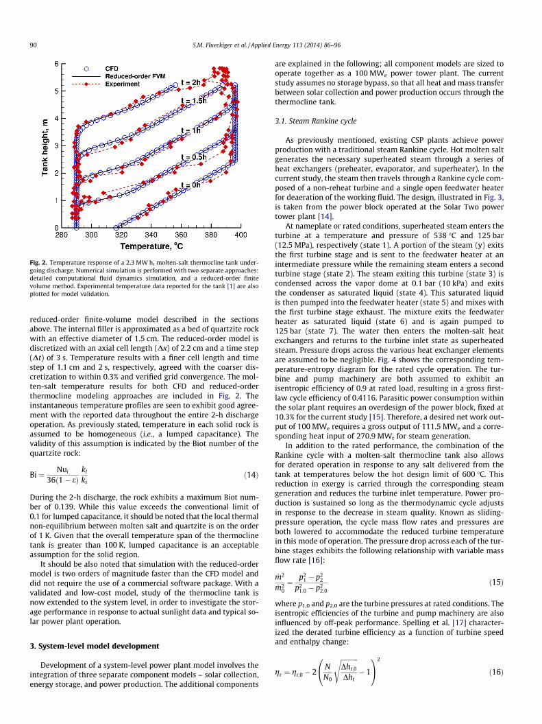
Fig. 2. Temperature response of a 2.3 MW ht molten-salt thermocline tank under-going discharge. Numerical simulation is performed with two separate approaches:detailed computational fluid dynamics simulation, and a reduced-order finitevolume method. Experimental temperature data reported for the tank [1] are alsoplotted for model validation.

90 S.M. Flueckiger et al. / Applied Energy 113 (2014) 86–96

reduced-order finite-volume model described in the sectionsabove. The internal filler is approximated as a bed of quartzite rockwith an effective diameter of 1.5 cm. The reduced-order model isdiscretized with an axial cell length (Dx) of 2.2 cm and a time step(Dt) of 3 s. Temperature results with a finer cell length and timestep of 1.1 cm and 2 s, respectively, agreed with the coarser dis-cretization to within 0.3% and verified grid convergence. The mol-ten-salt temperature results for both CFD and reduced-orderthermocline modeling approaches are included in Fig. 2. Theinstantaneous temperature profiles are seen to exhibit good agree-ment with the reported data throughout the entire 2-h dischargeoperation. As previously stated, temperature in each solid rock isassumed to be homogeneous (i.e., a lumped capacitance). Thevalidity of this assumption is indicated by the Biot number of thequartzite rock:

Bi ¼ Nui

36ð1� eÞkl

ksð14Þ

During the 2-h discharge, the rock exhibits a maximum Biot num-ber of 0.139. While this value exceeds the conventional limit of0.1 for lumped capacitance, it should be noted that the local thermalnon-equilibrium between molten salt and quartzite is on the orderof 1 K. Given that the overall temperature span of the thermoclinetank is greater than 100 K, lumped capacitance is an acceptableassumption for the solid region.

It should be also noted that simulation with the reduced-ordermodel is two orders of magnitude faster than the CFD model anddid not require the use of a commercial software package. With avalidated and low-cost model, study of the thermocline tank isnow extended to the system level, in order to investigate the stor-age performance in response to actual sunlight data and typical so-lar power plant operation.

3. System-level model development

Development of a system-level power plant model involves theintegration of three separate component models – solar collection,energy storage, and power production. The additional components

are explained in the following; all component models are sized tooperate together as a 100 MWe power tower plant. The currentstudy assumes no storage bypass, so that all heat and mass transferbetween solar collection and power production occurs through thethermocline tank.

3.1. Steam Rankine cycle

As previously mentioned, existing CSP plants achieve powerproduction with a traditional steam Rankine cycle. Hot molten saltgenerates the necessary superheated steam through a series ofheat exchangers (preheater, evaporator, and superheater). In thecurrent study, the steam then travels through a Rankine cycle com-posed of a non-reheat turbine and a single open feedwater heaterfor deaeration of the working fluid. The design, illustrated in Fig. 3,is taken from the power block operated at the Solar Two powertower plant [14].

At nameplate or rated conditions, superheated steam enters theturbine at a temperature and pressure of 538 �C and 125 bar(12.5 MPa), respectively (state 1). A portion of the steam (y) exitsthe first turbine stage and is sent to the feedwater heater at anintermediate pressure while the remaining steam enters a secondturbine stage (state 2). The steam exiting this turbine (state 3) iscondensed across the vapor dome at 0.1 bar (10 kPa) and exitsthe condenser as saturated liquid (state 4). This saturated liquidis then pumped into the feedwater heater (state 5) and mixes withthe first turbine stage exhaust. The mixture exits the feedwaterheater as saturated liquid (state 6) and is again pumped to125 bar (state 7). The water then enters the molten-salt heatexchangers and returns to the turbine inlet state as superheatedsteam. Pressure drops across the various heat exchanger elementsare assumed to be negligible. Fig. 4 shows the corresponding tem-perature-entropy diagram for the rated cycle operation. The tur-bine and pump machinery are both assumed to exhibit anisentropic efficiency of 0.9 at rated load, resulting in a gross first-law cycle efficiency of 0.4116. Parasitic power consumption withinthe solar plant requires an overdesign of the power block, fixed at10.3% for the current study [15]. Therefore, a desired net work out-put of 100 MWe requires a gross output of 111.5 MWe and a corre-sponding heat input of 270.9 MWt for steam generation.

In addition to the rated performance, the combination of theRankine cycle with a molten-salt thermocline tank also allowsfor derated operation in response to any salt delivered from thetank at temperatures below the hot design limit of 600 �C. Thisreduction in exergy is carried through the corresponding steamgeneration and reduces the turbine inlet temperature. Power pro-duction is sustained so long as the thermodynamic cycle adjustsin response to the decrease in steam quality. Known as sliding-pressure operation, the cycle mass flow rates and pressures areboth lowered to accommodate the reduced turbine temperaturein this mode of operation. The pressure drop across each of the tur-bine stages exhibits the following relationship with variable massflow rate [16]:

_m2

_m20

¼ p21 � p2

2

p21;0 � p2

2;0

ð15Þ

where p1,0 and p2,0 are the turbine pressures at rated conditions. Theisentropic efficiencies of the turbine and pump machinery are alsoinfluenced by off-peak performance. Spelling et al. [17] character-ized the derated turbine efficiency as a function of turbine speedand enthalpy change:

gt ¼ gt;0 � 2NN0

ffiffiffiffiffiffiffiffiffiffiffiDht;0

Dht

s� 1

0@

1A

2

ð16Þ

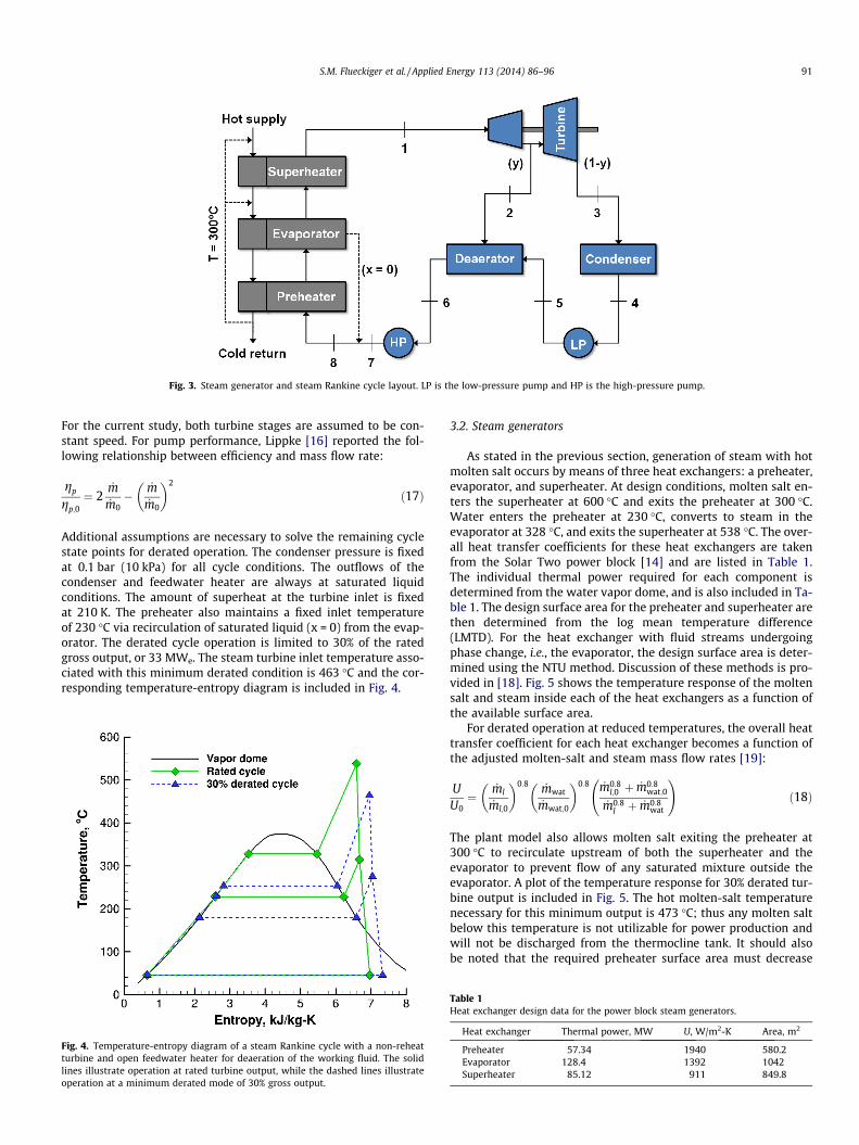
Fig. 3. Steam generator and steam Rankine cycle layout. LP is the low-pressure pump and HP is the high-pressure pump.

S.M. Flueckiger et al. / Applied Energy 113 (2014) 86–96 91

For the current study, both turbine stages are assumed to be con-stant speed. For pump performance, Lippke [16] reported the fol-lowing relationship between efficiency and mass flow rate:

gp

gp;0¼ 2

_m_m0�

_m_m0

� �2

ð17Þ

Additional assumptions are necessary to solve the remaining cyclestate points for derated operation. The condenser pressure is fixedat 0.1 bar (10 kPa) for all cycle conditions. The outflows of thecondenser and feedwater heater are always at saturated liquidconditions. The amount of superheat at the turbine inlet is fixedat 210 K. The preheater also maintains a fixed inlet temperatureof 230 �C via recirculation of saturated liquid (x = 0) from the evap-orator. The derated cycle operation is limited to 30% of the ratedgross output, or 33 MWe. The steam turbine inlet temperature asso-ciated with this minimum derated condition is 463 �C and the cor-responding temperature-entropy diagram is included in Fig. 4.

Fig. 4. Temperature-entropy diagram of a steam Rankine cycle with a non-reheatturbine and open feedwater heater for deaeration of the working fluid. The solidlines illustrate operation at rated turbine output, while the dashed lines illustrateoperation at a minimum derated mode of 30% gross output.

3.2. Steam generators

As stated in the previous section, generation of steam with hotmolten salt occurs by means of three heat exchangers: a preheater,evaporator, and superheater. At design conditions, molten salt en-ters the superheater at 600 �C and exits the preheater at 300 �C.Water enters the preheater at 230 �C, converts to steam in theevaporator at 328 �C, and exits the superheater at 538 �C. The over-all heat transfer coefficients for these heat exchangers are takenfrom the Solar Two power block [14] and are listed in Table 1.The individual thermal power required for each component isdetermined from the water vapor dome, and is also included in Ta-ble 1. The design surface area for the preheater and superheater arethen determined from the log mean temperature difference(LMTD). For the heat exchanger with fluid streams undergoingphase change, i.e., the evaporator, the design surface area is deter-mined using the NTU method. Discussion of these methods is pro-vided in [18]. Fig. 5 shows the temperature response of the moltensalt and steam inside each of the heat exchangers as a function ofthe available surface area.

For derated operation at reduced temperatures, the overall heattransfer coefficient for each heat exchanger becomes a function ofthe adjusted molten-salt and steam mass flow rates [19]:

UU0¼

_ml

_ml;0

� �0:8 _mwat

_mwat;0

� �0:8 _m0:8l;0 þ _m0:8

wat;0

_m0:8l þ _m0:8

wat

!ð18Þ

The plant model also allows molten salt exiting the preheater at300 �C to recirculate upstream of both the superheater and theevaporator to prevent flow of any saturated mixture outside theevaporator. A plot of the temperature response for 30% derated tur-bine output is included in Fig. 5. The hot molten-salt temperaturenecessary for this minimum output is 473 �C; thus any molten saltbelow this temperature is not utilizable for power production andwill not be discharged from the thermocline tank. It should alsobe noted that the required preheater surface area must decrease

Table 1Heat exchanger design data for the power block steam generators.

Heat exchanger Thermal power, MW U, W/m2-K Area, m2

Preheater 57.34 1940 580.2Evaporator 128.4 1392 1042Superheater 85.12 911 849.8

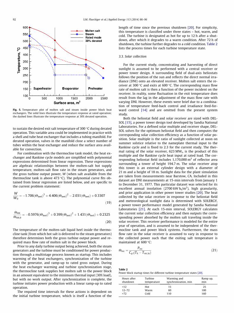
Fig. 5. Temperature plot of molten salt and steam inside power block heatexchangers. The solid lines illustrate the temperature response at rated operation;the dashed lines illustrate the temperature response at 30% derated operation.

92 S.M. Flueckiger et al. / Applied Energy 113 (2014) 86–96

to sustain the desired exit salt temperature of 300 �C during deratedoperation. This variable area could be implemented in practice witha shell and tube heat exchanger that includes a tubing manifold. Forderated operation, valves in the manifold close a select number oftubes within the heat exchanger and reduce the surface area avail-able for convection.

For combination with the thermocline tank model, the heat ex-changer and Rankine cycle models are simplified with polynomialexpressions determined from linear regression. These expressionsare algebraic relationships between the molten-salt hot supplytemperature, molten-salt flow rate in the steam generators, andthe gross turbine output power, W (when salt available from thethermocline tank is above 473 �C). The polynomial curve fits ob-tained from linear regression are listed below, and are specific tothe current problem statement:

WW0¼ �1:706 Hheelð Þ3 þ 4:406 Hheelð Þ2 � 2:031 Hheelð Þ þ 0:3307

ð19Þ

Table 2Power block startup times for different turbine temperature states [20].

Hours aftershutdown

Turbinetemperature

Warming andsynchronization, min

Ramp up,min

<12 Hot 15 2512–72 Warm 60 100>72 Cold 110 160

_mHX

_mHX;0¼ �0:5976ðHheelÞ3 þ 0:399ðHheelÞ2 þ 1:431ðHheelÞ þ 0:2325

ð20Þ

The temperature of the molten-salt liquid heel inside the thermo-cline tank (from which hot salt is delivered to the steam generators)therefore determines both the gross turbine output power and re-quired mass flow rate of molten salt in the power block.

Prior to any daily turbine output being achieved, both the steamgenerators and the turbine must be conditioned for power produc-tion through a multistage process known as startup. This includeswarming of the heat exchangers, synchronization of the turbinewith the generator, and ramp-up to rated gross output. Duringthe heat exchanger warming and turbine synchronization stage,the thermocline tank supplies hot molten salt to the power blockin an amount equivalent to the minimum thermal input (30% load),but with no work output. After synchronization is complete, theturbine initiates power production with a linear ramp-up to ratedoperation.

The required time intervals for these actions is dependent onthe initial turbine temperature, which is itself a function of the

length of time since the previous shutdown [20]. For simplicity,this temperature is classified under three states – hot, warm, andcold. The turbine is designated as hot for up to 12 h after a shut-down, after which it degrades to a warm condition. After 72 h ofshutdown, the turbine further degrades to a cold condition. Table 2lists the process times for each turbine temperature state.

3.3. Solar collection

For the current study, concentrating and harvesting of directsunlight is assumed to be performed with a central receiver orpower tower design. A surrounding field of dual-axis heliostatsfollows the position of the sun and reflects the direct normal irra-diance (DNI) onto an elevated receiver. Molten salt enters the re-ceiver at 300 �C and exits at 600 �C. The corresponding mass flowrate of molten salt is then a function of the power incident on thereceiver. In reality, some fluctuation in the exit temperature doesresult from the lag in the adjustment of the mass flow rate withvarying DNI. However, these events were brief due to a combina-tion of temperature feed-back control and irradiance feed-for-ward control [14] and are omitted from the present systemstudy.

Both the heliostat field and solar receiver are sized with DEL-SOL [15], a power tower design tool developed by Sandia NationalLaboratories. For a defined solar multiple and receiver shape, DEL-SOL solves for the optimum heliostat field and then computes thecorresponding solar collection efficiency as a function of solar po-sition. Solar multiple is the ratio of sunlight collected at noon onsummer solstice relative to the nameplate thermal input to theRankine cycle and is fixed to 2.3 for the current study. The ther-mal rating of the solar receiver, 623 MWt, is the product of thismultiple and the Rankine cycle heat input at rated load. The cor-responding heliostat field includes 1,170,000 m2 of reflector areasurrounding a tower of height 194.7 m. The solar receiver atopthis tower is an external cylinder design with a diameter of21 m and a height of 18 m. Sunlight data for the plant simulationare taken from measurements near Barstow, CA. Included in thisdataset are DNI measurements at 15-min intervals from January 1to December 31, 1977. This particular dataset was selected for itsexcellent annual insolation (2700 kW ht/m2), high granularity,and prior application in other power tower studies [20]. The heatcollected by the solar receiver in response to the heliostat fieldand meteorological sunlight data is determined with SOLERGY,a power tower performance model generated by Sandia NationalLaboratories [21]. At each 15-min interval, SOLERGY calculatesthe current solar collection efficiency and then outputs the corre-sponding power absorbed by the molten salt traveling inside thesolar receiver. This receiver performance is modeled for the entireyear of operation, and is assumed to be independent of the ther-mocline tank and power block systems. Furthermore, the massflow rate in the solar receiver is assumed to vary in response tothe collected power such that the exiting salt temperature ismaintained at 600 �C:

_mrec ¼Prec

Cp;lðTh � Trec;inÞð21Þ

S.M. Flueckiger et al. / Applied Energy 113 (2014) 86–96 93

3.4. Model integration

In the current study, the molten-salt thermocline tank is de-sired to provide the power tower plant with 6 h of thermal en-ergy storage. The maximum energy capacity of the tank shouldclearly exceed this condition to accommodate simultaneous con-tainment of salt at cold and transitional temperatures. Sizing ofthe storage system is informed by a previous design study ofthermocline tanks published by the Electric Power Research Insti-tute [22], which applied an approximate overdesign of 40% for thetank volume. The study also concluded that the molten-salt liquidlevel should not exceed 39 feet (11.89 m) to stay within the max-imum bearing capacity of the soil with a typical foundation. Theheight of the model quartzite bed is therefore fixed to 11 m toprovide additional volume for the liquid heel above the bed. Withthe given energy densities of the molten salt and quartzite rock, athermocline tank diameter of 36.27 m is required to satisfy therequisite energy capacity and volumetric overdesign. The effectivediameter of the quartzite rock granules inside the tank is fixed to1 cm [23].

Integrating the thermocline tank model with the additionalcomponent models previously described generates a system-levelmodel of a 100 MWe power tower plant. The individual modelsinteract at the system level as follows. During daylight hours, mol-ten salt picks up solar radiation incident on the receiver and isdelivered to the thermocline tank heel. The amount of heat inputavailable at each time step is obtained from the SOLERGY receiveranalysis. When the thermocline tank contains enough energy tosustain 2 h of steam generation in the heat exchangers, hot saltis sent to the power block to initiate turbine startup. After startupis complete, the turbine is set for rated power production. Cold saltexiting the power block either returns to the solar receiver or to thebottom of the tank, as dictated by mass balance in the solar collec-tion loop.

It is again noted that no provision for a bypass loop is included be-tween the solar receiver and the power block, and all heat and masstransport in the power plant is routed through the thermocline tank.The thermocline tank operating condition (charge, discharge, orstandby) and corresponding salt flow direction is therefore depen-dent on the immediate disparity in molten-salt mass flow rate be-tween the power block (Eq. (20)) and the solar receiver (Eq. (21)).For example, when the receiver provides hot salt at a faster rate thanis necessary in the power block, the thermocline tank is charged withthe excess. Conversely, when the power block requires more flowthan the amount provided by the receiver, the tank undergoes a dis-charge to make up the difference. A standby condition with stagnantmolten salt (i.e., no net flow inside the porous bed) occurs when thedischarging tank is depleted of all usable energy.

For prolonged charge processes, the salt exiting the bottom ofthe thermocline tank will begin to increase in temperature as thetransitional heat-exchange region reaches the tank floor. Whenthis warmer salt enters the solar receiver, the receiver mass flowrate increases to maintain the exit hot temperature at 600 �C, gov-erned by Eq. (21). However, cold salt exiting the bottom of thethermocline tank is limited to a maximum allowable temperatureof 400 �C to prevent overcharging of the storage system. Above thistemperature, the thermocline tank is declared to be at energycapacity and transitions to a forced standby condition. With nomore available storage, the solar receiver can only collect enoughenergy to satisfy the Rankine cycle steam generation. Heliostatsare defocused away from the receiver and some amount of sunlightavailable for collection must be forgone: this amount of energy isknown as thermal energy discard. The forced tank standby persistsuntil the solar receiver power output decays near sunset and theenergy-saturated tank can then be discharged to sustain the ratedpower production.

Under ideal clear sky conditions on a given day, the thermoclinetank would energize to its capacity, go into standby, and finally dis-charge near sunset following shutdown of the solar receiver. Inreality, random cloud transients will lead to sporadic DNI lossesduring daylight hours. Therefore additional care must be taken inthe operation of the thermocline tank to avoid chaotic flow direc-tion changes and consequent wear on the turbine. In the operationconsidered in the current study, dispatch of hot molten salt fromthe thermocline tank to the power block is prohibited until the tur-bine is guaranteed to operate for at least 2 h. Prior to turbine start-up, the system model checks both the energy content of the tank aswell as receiver performance in the immediate future (alreadyknown from the SOLERGY solution) to ensure that this conditionon the turbine is satisfied. The authors assume that in practice,plant operators are capable of making similar near-term receiverpredictions from weather forecasts. As a result, rapid on–off tog-gling of either the thermocline tank or the Rankine cycle is avoided.

4. Results and discussion

4.1. CSP plant performance with and without storage

At the onset of the power plant simulation, the thermoclinetank fillerbed and liquid heel are both initialized to the cold mol-ten-salt temperature limit of 300 �C. The fillerbed geometry is dis-cretized with a cell length of 2.2 cm (500 cells) and a time step of3 s; grid independence at this resolution was already verified withthe previous simulation of a small-scale thermocline tank. As sta-ted before, the performance of the heliostat field and solar receiveris first simulated in SOLERGY using a meteorological year of sun-light data reported near Barstow, CA. The amount of power col-lected by the receiver then serves as an input to the integratedthermocline tank and power block models for each time step ofsimulation.

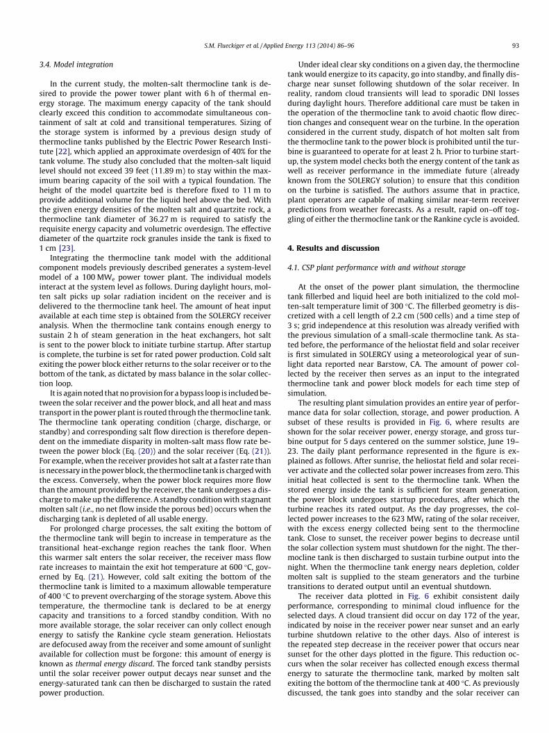
The resulting plant simulation provides an entire year of perfor-mance data for solar collection, storage, and power production. Asubset of these results is provided in Fig. 6, where results areshown for the solar receiver power, energy storage, and gross tur-bine output for 5 days centered on the summer solstice, June 19–23. The daily plant performance represented in the figure is ex-plained as follows. After sunrise, the heliostat field and solar recei-ver activate and the collected solar power increases from zero. Thisinitial heat collected is sent to the thermocline tank. When thestored energy inside the tank is sufficient for steam generation,the power block undergoes startup procedures, after which theturbine reaches its rated output. As the day progresses, the col-lected power increases to the 623 MWt rating of the solar receiver,with the excess energy collected being sent to the thermoclinetank. Close to sunset, the receiver power begins to decrease untilthe solar collection system must shutdown for the night. The ther-mocline tank is then discharged to sustain turbine output into thenight. When the thermocline tank energy nears depletion, coldermolten salt is supplied to the steam generators and the turbinetransitions to derated output until an eventual shutdown.

The receiver data plotted in Fig. 6 exhibit consistent dailyperformance, corresponding to minimal cloud influence for theselected days. A cloud transient did occur on day 172 of the year,indicated by noise in the receiver power near sunset and an earlyturbine shutdown relative to the other days. Also of interest isthe repeated step decrease in the receiver power that occurs nearsunset for the other days plotted in the figure. This reduction oc-curs when the solar receiver has collected enough excess thermalenergy to saturate the thermocline tank, marked by molten saltexiting the bottom of the thermocline tank at 400 �C. As previouslydiscussed, the tank goes into standby and the solar receiver can

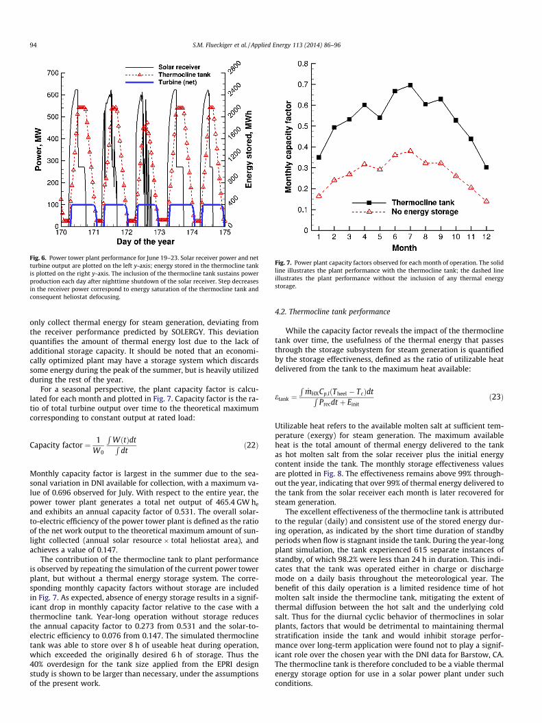
Fig. 6. Power tower plant performance for June 19–23. Solar receiver power and netturbine output are plotted on the left y-axis; energy stored in the thermocline tankis plotted on the right y-axis. The inclusion of the thermocline tank sustains powerproduction each day after nighttime shutdown of the solar receiver. Step decreasesin the receiver power correspond to energy saturation of the thermocline tank andconsequent heliostat defocusing.

Fig. 7. Power plant capacity factors observed for each month of operation. The solidline illustrates the plant performance with the thermocline tank; the dashed lineillustrates the plant performance without the inclusion of any thermal energystorage.

94 S.M. Flueckiger et al. / Applied Energy 113 (2014) 86–96

only collect thermal energy for steam generation, deviating fromthe receiver performance predicted by SOLERGY. This deviationquantifies the amount of thermal energy lost due to the lack ofadditional storage capacity. It should be noted that an economi-cally optimized plant may have a storage system which discardssome energy during the peak of the summer, but is heavily utilizedduring the rest of the year.

For a seasonal perspective, the plant capacity factor is calcu-lated for each month and plotted in Fig. 7. Capacity factor is the ra-tio of total turbine output over time to the theoretical maximumcorresponding to constant output at rated load:

Capacity factor ¼ 1W0

RWðtÞdtR

dtð22Þ

Monthly capacity factor is largest in the summer due to the sea-sonal variation in DNI available for collection, with a maximum va-lue of 0.696 observed for July. With respect to the entire year, thepower tower plant generates a total net output of 465.4 GW he

and exhibits an annual capacity factor of 0.531. The overall solar-to-electric efficiency of the power tower plant is defined as the ratioof the net work output to the theoretical maximum amount of sun-light collected (annual solar resource � total heliostat area), andachieves a value of 0.147.

The contribution of the thermocline tank to plant performanceis observed by repeating the simulation of the current power towerplant, but without a thermal energy storage system. The corre-sponding monthly capacity factors without storage are includedin Fig. 7. As expected, absence of energy storage results in a signif-icant drop in monthly capacity factor relative to the case with athermocline tank. Year-long operation without storage reducesthe annual capacity factor to 0.273 from 0.531 and the solar-to-electric efficiency to 0.076 from 0.147. The simulated thermoclinetank was able to store over 8 h of useable heat during operation,which exceeded the originally desired 6 h of storage. Thus the40% overdesign for the tank size applied from the EPRI designstudy is shown to be larger than necessary, under the assumptionsof the present work.

4.2. Thermocline tank performance

While the capacity factor reveals the impact of the thermoclinetank over time, the usefulness of the thermal energy that passesthrough the storage subsystem for steam generation is quantifiedby the storage effectiveness, defined as the ratio of utilizable heatdelivered from the tank to the maximum heat available:

etank ¼R

_mHXCp;lðTheel � TcÞdtRPrecdt þ Einit

ð23Þ

Utilizable heat refers to the available molten salt at sufficient tem-perature (exergy) for steam generation. The maximum availableheat is the total amount of thermal energy delivered to the tankas hot molten salt from the solar receiver plus the initial energycontent inside the tank. The monthly storage effectiveness valuesare plotted in Fig. 8. The effectiveness remains above 99% through-out the year, indicating that over 99% of thermal energy delivered tothe tank from the solar receiver each month is later recovered forsteam generation.

The excellent effectiveness of the thermocline tank is attributedto the regular (daily) and consistent use of the stored energy dur-ing operation, as indicated by the short time duration of standbyperiods when flow is stagnant inside the tank. During the year-longplant simulation, the tank experienced 615 separate instances ofstandby, of which 98.2% were less than 24 h in duration. This indi-cates that the tank was operated either in charge or dischargemode on a daily basis throughout the meteorological year. Thebenefit of this daily operation is a limited residence time of hotmolten salt inside the thermocline tank, mitigating the extent ofthermal diffusion between the hot salt and the underlying coldsalt. Thus for the diurnal cyclic behavior of thermoclines in solarplants, factors that would be detrimental to maintaining thermalstratification inside the tank and would inhibit storage perfor-mance over long-term application were found not to play a signif-icant role over the chosen year with the DNI data for Barstow, CA.The thermocline tank is therefore concluded to be a viable thermalenergy storage option for use in a solar power plant under suchconditions.

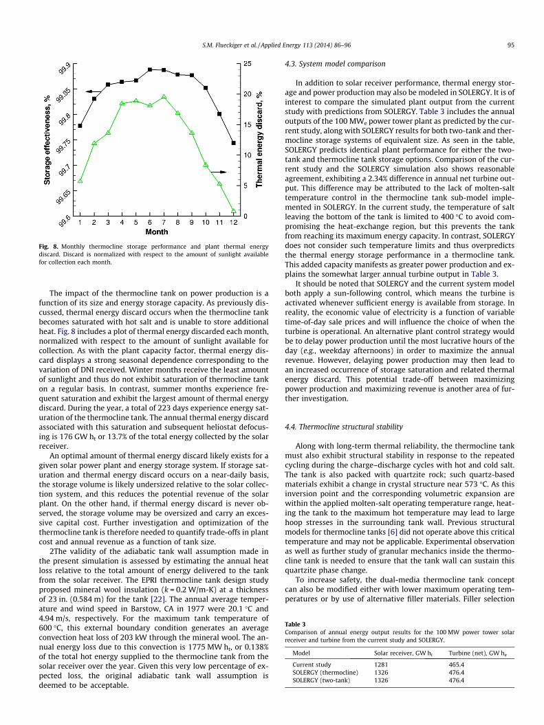
Fig. 8. Monthly thermocline storage performance and plant thermal energydiscard. Discard is normalized with respect to the amount of sunlight availablefor collection each month.

Table 3Comparison of annual energy output results for the 100 MW power tower solarreceiver and turbine from the current study and SOLERGY.

Model Solar receiver, GW ht Turbine (net), GW he

Current study 1281 465.4SOLERGY (thermocline) 1326 476.4SOLERGY (two-tank) 1326 476.4

S.M. Flueckiger et al. / Applied Energy 113 (2014) 86–96 95

The impact of the thermocline tank on power production is afunction of its size and energy storage capacity. As previously dis-cussed, thermal energy discard occurs when the thermocline tankbecomes saturated with hot salt and is unable to store additionalheat. Fig. 8 includes a plot of thermal energy discarded each month,normalized with respect to the amount of sunlight available forcollection. As with the plant capacity factor, thermal energy dis-card displays a strong seasonal dependence corresponding to thevariation of DNI received. Winter months receive the least amountof sunlight and thus do not exhibit saturation of thermocline tankon a regular basis. In contrast, summer months experience fre-quent saturation and exhibit the largest amount of thermal energydiscard. During the year, a total of 223 days experience energy sat-uration of the thermocline tank. The annual thermal energy discardassociated with this saturation and subsequent heliostat defocus-ing is 176 GW ht or 13.7% of the total energy collected by the solarreceiver.

An optimal amount of thermal energy discard likely exists for agiven solar power plant and energy storage system. If storage sat-uration and thermal energy discard occurs on a near-daily basis,the storage volume is likely undersized relative to the solar collec-tion system, and this reduces the potential revenue of the solarplant. On the other hand, if thermal energy discard is never ob-served, the storage volume may be oversized and carry an exces-sive capital cost. Further investigation and optimization of thethermocline tank is therefore needed to quantify trade-offs in plantcost and annual revenue as a function of tank size.

2The validity of the adiabatic tank wall assumption made inthe present simulation is assessed by estimating the annual heatloss relative to the total amount of energy delivered to the tankfrom the solar receiver. The EPRI thermocline tank design studyproposed mineral wool insulation (k = 0.2 W/m-K) at a thicknessof 23 in. (0.584 m) for the tank [22]. The annual average temper-ature and wind speed in Barstow, CA in 1977 were 20.1 �C and4.94 m/s, respectively. For the maximum tank temperature of600 �C, this external boundary condition generates an averageconvection heat loss of 203 kW through the mineral wool. The an-nual energy loss due to this convection is 1775 MW ht, or 0.138%of the total hot energy supplied to the thermocline tank from thesolar receiver over the year. Given this very low percentage of ex-pected loss, the original adiabatic tank wall assumption isdeemed to be acceptable.

4.3. System model comparison

In addition to solar receiver performance, thermal energy stor-age and power production may also be modeled in SOLERGY. It is ofinterest to compare the simulated plant output from the currentstudy with predictions from SOLERGY. Table 3 includes the annualoutputs of the 100 MWe power tower plant as predicted by the cur-rent study, along with SOLERGY results for both two-tank and ther-mocline storage systems of equivalent size. As seen in the table,SOLERGY predicts identical plant performance for either the two-tank and thermocline tank storage options. Comparison of the cur-rent study and the SOLERGY simulation also shows reasonableagreement, exhibiting a 2.34% difference in annual net turbine out-put. This difference may be attributed to the lack of molten-salttemperature control in the thermocline tank sub-model imple-mented in SOLERGY. In the current study, the temperature of saltleaving the bottom of the tank is limited to 400 �C to avoid com-promising the heat-exchange region, but this prevents the tankfrom reaching its maximum energy capacity. In contrast, SOLERGYdoes not consider such temperature limits and thus overpredictsthe thermal energy storage performance in a thermocline tank.This added capacity manifests as greater power production and ex-plains the somewhat larger annual turbine output in Table 3.

It should be noted that SOLERGY and the current system modelboth apply a sun-following control, which means the turbine isactivated whenever sufficient energy is available from storage. Inreality, the economic value of electricity is a function of variabletime-of-day sale prices and will influence the choice of when theturbine is operational. An alternative plant control strategy wouldbe to delay power production until the most lucrative hours of theday (e.g., weekday afternoons) in order to maximize the annualrevenue. However, delaying power production may then lead toan increased occurrence of storage saturation and related thermalenergy discard. This potential trade-off between maximizingpower production and maximizing revenue is another area of fur-ther investigation.

4.4. Thermocline structural stability

Along with long-term thermal reliability, the thermocline tankmust also exhibit structural stability in response to the repeatedcycling during the charge–discharge cycles with hot and cold salt.The tank is also packed with quartzite rock; such quartz-basedmaterials exhibit a change in crystal structure near 573 �C. As thisinversion point and the corresponding volumetric expansion arewithin the applied molten-salt operating temperature range, heat-ing the tank to the maximum hot temperature may lead to largehoop stresses in the surrounding tank wall. Previous structuralmodels for thermocline tanks [6] did not operate above this criticaltemperature and may not be applicable. Experimental observationas well as further study of granular mechanics inside the thermo-cline tank is needed to ensure that the tank wall can sustain thisquartzite phase change.

To increase safety, the dual-media thermocline tank conceptcan also be modified either with lower maximum operating tem-peratures or by use of alternative filler materials. Filler selection

96 S.M. Flueckiger et al. / Applied Energy 113 (2014) 86–96

for the solid rock calls for both low cost and physical stability un-der repeated thermal cycling. In addition to quartzite, Pachecoet al. [1] reported successful application of iron ore taconite pelletswith molten salt. However, physical property data for taconite arenot readily available in the literature and require further study.Additional materials not considered in [1] should also be explored.

5. Conclusions

A numerical model for molten-salt thermocline tank operationhas been developed to provide accurate simulation of mass and en-ergy transport at low computing cost and without reliance on com-mercial CFD software. The thermal model is integrated into asystem-level simulation of a 100 MWe power tower plant to assessthermocline tank performance under realistic and long-term oper-ating conditions. Operation of the plant model is informed by ameteorological year of sunlight data recorded near Barstow, CAin 1977. The molten-salt thermocline tank, sized to provide 6 hof thermal energy storage, increased the annual plant capacity fac-tor to 0.531 with excellent year-long storage effectiveness exceed-ing 99%. This good performance results from the regular andconsistent utilization of the stored energy in the tank duringyear-long plant operation, limiting the residence time of hot saltinside the tank and the corresponding loss of thermal stratificationthat would result. Comparison of the model developed in this workwith the results from SOLERGY showed excellent agreement. Addi-tional study is needed to assess the optimum tank size that bal-ances the solar collection system size with the economic impactof turbine delay on maximum hourly electricity prices.

Even if long-term thermal stability is achieved, structural integ-rity of the thermocline tank remains a design concern due to thelarge volumetric expansion of the quartzite rock at elevated moltensalt temperatures relative to the surrounding tank wall. Furtherinvestigation is needed to determine the maximum safe operatingtemperatures for quartzite rock and also to identify suitable alter-native, non-quartz filler candidate materials.

Acknowledgements

Sandia National Laboratories is a multi-program laboratorymanaged and operated by Sandia Corporation, a wholly ownedsubsidiary of Lockheed Martin Corporation, for the U.S. Depart-ment of Energy’s National Nuclear Security Administration undercontract DE-AC04-94AL85000. The authors acknowledge Brian D.Ehrhart for assistance with use of models in DELSOL and SOLERGY.

References

[1] Pacheco JE, Showalter SK, Kolb WJ. Development of a molten-salt thermoclinethermal storage system for parabolic trough plants. ASME J Sol Energy Eng2002;124:153–9.

[2] Radosevich LG. Final report on the power production phase of the 10 MWe

solar central receiver pilot plant. SAND87-8022. Sandia National Laboratories;1988.

[3] Yang Z, Garimella SV. Thermal analysis of solar thermal energy storage in amolten-salt thermocline. Sol Energy 2010;84:974–85.

[4] Yang Z, Garimella SV. Molten-salt thermal energy storage in thermoclinesunder different environmental boundary conditions. Appl Energy 2010;87:3322–9.

[5] Xu C, Wang Z, He Y, Li X, Bai F. Sensitivity analysis of the numerical study onthe thermal performance of a packed-bed molten salt thermocline thermalstorage system. Appl Energy 2012;92:65–75.

[6] Flueckiger S, Yang Z, Garimella SV. An integrated thermal and mechanicalinvestigation of molten-salt thermocline energy storage. Appl Energy 2011;88:2098–105.

[7] Van Lew JT, Li P, Chan CL, Karaki W, Stephens J. Analysis of heat storage anddelivery of a thermocline tank having solid filler material. ASME J Sol EnergyEng 2011;133:021003.

[8] Kolb GJ. Evaluation of annual performance of 2-tank and thermoclinethermal storage systems for trough plants. ASME J Sol Energy Eng 2011;133:031023.

[9] Nissen DA. Thermophysical properties of the equimolar mixture NaNO3–KNO3

from 300C to 600C. J Chem Eng Data 1982;27:269–73.[10] Pacheco JE, Ralph ME, Chavez JM, Dunkin SR, Rush EE, Ghanbari CH, et al.

Results of molten salt panel and component experiments for solar centralreceivers. SAND94-2525. Sandia National Laboratories; 1995.

[11] Cote J, Konrad J-M. Thermal conductivity of base-coarse materials. CanGeotech J 2005;42:61–78.

[12] Gonzo EE. Estimating correlations for the effective thermal conductivity ofgranular materials. Chem Eng J 2002;90:299–302.

[13] Wakao N, Kaguei S. Heat and mass transfer in packed beds. New York: GordonBeach; 1982.

[14] Pacheco JE. Final test and evaluation results from the solar two project.SAND2002-0120. Sandia National Laboratories; 2002.

[15] Kistler BL. A user’s manual for DELSOL3. SAND86-8018. Sandia NationalLaboratories; 1986.

[16] Lippke F. Simulation of the part-load behavior of a 30 MWe SEGS plant.SAND95-1293. Sandia National Laboratories; 1995.

[17] Spelling J, Jocker M, Martin A. Thermal modeling of a solar steam turbine witha focus on start-up time reduction. ASME J Eng Gas Turbines Power2012;134:013001.

[18] Incropera FP, DeWitt DP. Fundamentals of heat and mass transfer. 5th ed. JohnWiley & Sons; 2002.

[19] Patnode AM. Simulation and performance evaluation of parabolic trough solarpower plants. MSME Thesis. University of Wisconsin-Madison, 2006.

[20] Kolb GJ. An evaluation of possible next-generation high-temperaturemolten-salt power towers. SAND2011-9320. Sandia National Laboratories;2011.

[21] Stoddard MC, Faas SE, Chiang CJ, Dirks JA. SOLERGY. SAND86-8060. SandiaNational Laboratories; 1987.

[22] Electric Power Research Institute. Solar thermal storage systems: preliminarydesign study. 1019581. EPRI; 2010.

[23] Flueckiger SM, Garimella SV. Second-law analysis of molten-salt thermalenergy storage in thermoclines. Sol Energy 2012;86:1621–31.