Supplementary Information A Salt-Rejecting, Floating Solar ...

1
Solar Energy Generation in Three Dimensions:
Supplementary Information
Marco Bernardi, Nicola Ferralis, Jin H. Wan, Rachelle Villalon,
and Jeffrey C. Grossman
The supplementary information is divided into two main sections, covering respectively:
1 – Methods and Materials
2 – Supplementary Text, further divided into:
2.1 – 3DPV computer code, optimization, and validation
2.2 – Details of all simulations
2.3 – Power balancing and weather effects
2.4 – Examples of applications of 3DPV
1. METHODS AND MATERIALS
The 3DPV structures were fabricated using commercially available Si solar cells
purchased from Solarbotics (type SCC3733, 37x33mm, monocrystalline Si) with nominal
open-circuit voltage and short-circuit current of 6.7 V and 20 mA, respectively, and
AM1.5 efficiency of 10 % verified independently with a solar simulator. The Si active
layer is protected by a 1 mm epoxy layer with refractive index n = 1.6 that yields an
overall cell reflectivity at normal incidence R ≈ 14 %. The panels were mounted onto a
3D-printed plastic frame for the particular structure of choice, and electrically connected
in parallel through a main parallel bus, with blocking diodes placed in series with each
Electronic Supplementary Material (ESI) for Energy & Environmental ScienceThis journal is © The Royal Society of Chemistry 2012

2
cell. 3D-printed frames were realized using Fused Deposition Modeling (FDM)
manufacturing technology with strict tolerances (0.005"), in a 3D printer purchased from
Stratasys Inc. Frame models were realized in acrylonitrile butadiene styrene polymer starting from a 3D digital polygon mesh of the object. The same 3D digital files were
converted into input files with proper format for the 3DPV computer code, thus allowing
us to simulate 3DPV structures identical to those fabricated experimentally. This method
is flexible and can be adapted to manufacture arbitrary shapes. The indoor
characterization of the 3DPV structures was performed using a solar simulator with a
1300 W xenon arc lamp (Newport Corporation, model 91194) fitted with a global AM
1.5 filter and calibrated to 1000 W/m2 intensity. In order to perform angle-dependent
measurements of the current-voltage characteristics, solar panels were mounted on
supports with predetermined angles to allow adjustment of the orientation with respect to
the incoming light. Since commonly employed solar simulators are designed to operate at
a very well defined distance between the light source and the tested flat panel, any
variation of such distance has a significant effect on the illumination intensity and thus on
the power output, which made outdoor testing necessary for accurate results for all 3D
shapes. The outdoor solar cell characterization was performed in Cambridge on the roof
of building 13 of the MIT campus during the months from June to December 2011. Up to
four structures (including a flat panel used for reference) were tested simultaneously
during each session to allow direct comparisons independent of weather conditions. The
orientation of the structures was carefully checked with the use of a compass. The
current-voltage characteristics were measured at time intervals of 12–15 min using a
custom-made,24 battery operated automatic acquisition system, controlled by an Arduino
Electronic Supplementary Material (ESI) for Energy & Environmental ScienceThis journal is © The Royal Society of Chemistry 2012

3
MEGA 2560 microcontroller. The data were stored in an SD-type memory card for
further analysis.
2. SUPPLEMENTARY TEXT
2.1 – 3DPV COMPUTER CODE, OPTIMIZATION, AND VALIDATION
Energy calculation.
The main routine of our code performs calculations of the total energy absorbed
during any given period of time and at any given location on Earth by a 3D assembly of
panels of given reflectivity and power conversion efficiency. This routine incorporates
key differences compared to the one used in Ref. 5. For example, the use of Air Mass
(AM) correction for solar flux allows for simulations during different seasons and at
different latitudes, with a reliable calculation of power curves and total energy. The
computation has been generalized to account for cells of different efficiency and
reflectivity within the structure, thus expanding the design opportunities to systems such
as solar energy concentrators, where the mirrors are added as cells with zero efficiency
and 100% reflectivity. The code has also been extended to incorporate a start and an end
date, so that simulations over any interval of time are possible. The Fresnel equations
employed now assume unpolarized sunlight. All aspects of the code were carefully tested
(see below), and new optimization methods were added to find energy maxima as
discussed below.
Our algorithm considers a 3D assembly of N panels of arbitrary efficiency and
optical properties, where the lth panel has refractive index nl and conversion efficiency ηl
Electronic Supplementary Material (ESI) for Energy & Environmental ScienceThis journal is © The Royal Society of Chemistry 2012

4
(l = 1, 2, …, N, and ηl = 0 for mirrors). The energy E (kWh/day) generated in a given day
and location can be computed as:
where Δt is a time-step (in hours) in the solar trajectory allowing for converged energy,
and Pk is the total power generated at the kth solar time-step. The total energy over a
period of time is obtained by looping over the days composing the time period, and
summing the energies generated during each day.
The key quantity Pk can be expanded perturbatively:
where the mth term accounts for m reflections of a light ray that initially hits the structure
– and is thus of order Rm, where R is the average reflectivity of the absorbers – so that for
most cases of practical interest, an expansion up to m = 1 suffices.
Explicitly, Pk(0) and Pk
(1) can be written as:
where Ik is the incident energy flux from the Sun at the kth time-step (and includes a
correction for Air-Mass effects), Al,eff is the unshaded area of the lth cell, and Rl (θl,k) is the
Electronic Supplementary Material (ESI) for Energy & Environmental ScienceThis journal is © The Royal Society of Chemistry 2012
5
reflectivity of the lth cell for an incidence angle (from the local normal) θl,k at the kth time-
step, that is calculated through the Fresnel equations for unpolarized incident light. In eq.
(2) the residual power after the absorption of direct sunlight (first square bracket) is
transmitted from the lth cell and redirected with specular reflection to the sth cell that gets
first hit by the reflected ray. The sth cell absorbs it according to its efficiency ηs and to its
reflectivity calculated using the angle of incidence αls,k with the reflected ray. In practice,
both formulas are computed by setting up a fine converged grid for each cell (normally g
=10,000 grid-points) so that all quantities are computed by looping over sub-cells of area
equal to A / g (A is the area of a given triangular cell area), which also removes the need
to sum s over the subset of cells hit by the reflected light coming out of a given cell.
The empirical expression used to calculate the intensity of incident light on the
Earth’s surface Ik (W/m2) with AM correction for the Sun’s position at the kth time-step
is:25
where βk is the Zenith angle of the sun ray with the Earth’s local normal at the kth solar
time-step, 1353 W/m2 is the solar constant, the factor 1.1 takes into account (though in an
elementary way) diffuse radiation, and the third factor contains the absorption from the
atmosphere and an empirical AM correction. The angle βk is calculated at each step of the
Sun’s trajectory for the particular day and location using a solar vector obtained from the
solar position algorithm developed by Reda et al.11 and incorporated into our code.
Dispersion effects (dependence of optical properties on radiation wavelength) and
weather conditions are not taken into account in the simulations and are the main
approximations of our model. Dispersion effects are difficult to include, and would
Electronic Supplementary Material (ESI) for Energy & Environmental ScienceThis journal is © The Royal Society of Chemistry 2012

6
increase the computation time by a factor of 10–100. Weather effects require reliable
weather information (e.g. from satellites), and would be interesting to explore in light of
recent work on optimization of PV output based on weather by Lave et al,26 as well as
our own experimental measurements.
Optimization algorithms.
Our code uses genetic algorithm (GA) and simulated-annealing Monte Carlo
(MC) methods to maximize the energy E generated in a given day in the phase space
constituted by the panels’ coordinates. The GA algorithm was used as described in Ref.
5. Briefly, candidate 3D structures are combined using operations based on three
principles of natural selection (selection, recombination, and mutation), using a GA
algorithm adapted from Ref. 16. The “tournament without replacement” selection scheme
was used,27 in which s structures from the current population are chosen randomly and
the one of highest fitness proceeds to the mating pool, until a desired pool size is reached.
In our simulations s = 2, and the fitness function corresponds to the energy produced in
one day by the given structure.
The recombination step randomly combines 3D structures in the mating pool and
with some probability (here 80%) crosses their triangle coordinates, causing the swapping
of whole triangles. A two-point crossover recombination method was employed, wherein
two indices are selected at random in the list of coordinates composing the chromosomes,
and then the entire string of coordinates in between is traded between the pair of
solutions.
Electronic Supplementary Material (ESI) for Energy & Environmental ScienceThis journal is © The Royal Society of Chemistry 2012

7
Finally, the mutation operator slightly perturbs each coordinate, for the purpose of
searching more efficiently the coordinates space. These three operations are performed
until convergence is reached (usually 10,000–50,000 simulation steps), and a 3DPV
structure with maximal energy production is achieved. The number of grid-points per
triangular cell was fixed to 100 during most optimizations to limit computation time, and
following the optimization optimal structures were re-examined using 10,000 grid-points
as in all other simulations.
The MC algorithm was used to optimize structures of mixed optical properties,
where we chose trial moves that preserve the optical properties of the single cells to favor
the convergence of the optimization process. Our MC algorithm uses a standard
Metropolis scheme for acceptance/rejection of trial moves, and a fictitious temperature T
that is decreased during the simulation according to a specified cooling schedule.13 Trial
moves consisted in the change of a randomly chosen set of coordinates of the candidate
structure. A number of coordinates varying between 1 and 9N (N is the number of
triangles) were translated randomly within a cubic box of side 1–100 % the simulation
box side (with periodic boundary conditions), thus determining a change ΔE in the total
energy. When ΔE >0 the move is accepted, whereas when ΔE <0 the move is accepted
with probability
.
When a move is accepted, the structure is updated and a new random move is
performed. Most MC simulations consisted of 100,000 steps with a converged value of
Electronic Supplementary Material (ESI) for Energy & Environmental ScienceThis journal is © The Royal Society of Chemistry 2012

8
the final energy. The code implements both power law and inverse-log cooling
schedules;13 in most simulations we used the inverse-log cooling schedule
.
Average ΔE values for the given trial move were determined prior to running the
optimization with a short simulation (1000 steps). Parameters for the cooling schedule
were determined by imposing a temperature value such that the initial acceptance rate is
P=0.99 and the final acceptance is P=10-5, with a method detailed in Ref. 14.
The GA and MC algorithms gave consistent results for optimization of 1, 2, 3, 4, 10, 20,
50 cells in a 10x10x10 m3 cubic simulation box (not shown here), suggesting that both
algorithms are capable of finding energy values near the global maximum using less than
100,000 steps. Since the main cost of the simulation is the energy computation routine,
the cost is comparable for both algorithms. For example, a 100,000 steps long simulation
with 20 cells is completed in 1–2 days on a single processor. Parallelization of the code
using a standard MPI library is possible and would cut the computation time by a factor
linear in the number of processors.
Validation tests.
The reliability of our code was checked using a large number of tests in a
multitude of conditions, some of which are reported here and in the paper. Computation
of the inter-cell shading and reflected energy was tested using the structure and Sun
trajectory shown in Fig. S1a. In a day and location where the apparent Sun trajectory
goes from East to West keeping a 90° (or 270°) azimuth angle at all times (e.g. Sept. 19
at latitude 1°, longitude -71°, and GMC time -5),12 a tall wall (50 m height) was placed
Electronic Supplementary Material (ESI) for Energy & Environmental ScienceThis journal is © The Royal Society of Chemistry 2012

9
vertical to the ground, and a small square mirror (1 m side) was placed 10 m away from
the wall and tilted so as to completely reflect incident light to the middle height of the
wall when the Sun is at the Zenith (11:35AM for our case). Until the Sun position moves
over the wall, the mirrors are shaded; they only start receiving light at approximately
11AM, and then continue reflecting light to the wall almost until the sunset. Comparison
is made in Fig. S1b between the power generated at different times of the day for the two
following cases:
1- the wall does not generate energy (its efficiency is set to zero), and the small mirror
cells absorb and convert all incident light with unit efficiency (blue curve);
2- the wall absorbs all of the incident light, both reflected by the mirrors (here with zero
conversion efficiency) and from direct incident sunlight. For this case, the difference in
power with and without mirrors is calculated, and represents the gain due to energy
transferred by the mirrors and absorbed by the wall (red curve).
Fig. S1 (a) Tested trajectory (red dots) re-scaled by a factor of 200,000. The wall is shown in green, and the
mirrors indicated by the arrow. (b) Comparison of expected and calculated power contribution from the
mirror, validating our reflection and shading algorithms.
Electronic Supplementary Material (ESI) for Energy & Environmental ScienceThis journal is © The Royal Society of Chemistry 2012

10
Cases 1 and 2 should yield almost identical power values at all times between
11AM and sunset, since geometrical optics imposes that rays incident on the mirrors are
reflected completely to the wall in this situation, and the power incident on the mirrors
(expected contribution, blue curve in Fig. S1b) is transferred and absorbed completely by
the wall. In addition, shading of the small mirrors is expected to occur almost until
11AM. The excellent matching observed in Fig. S1b between the predicted and observed
curve in the useful time interval demonstrates that the code can calculate reliably both
shading and reflection effects.
For further validation, Sun’s trajectories returned by the code were compared with
those provided in Ref. 13. The inclination and azimuth angles match the expected ones
within 1% in all tested cases. The code can also match very well values of solar
insolation from tables for locations where weather is not an important variable, since no
weather correction is taken into account in our code. Fig. S2 shows a comparison
between the simulated ground insolation on the 15th day of each calendar month -
obtained from simulation of a flat horizontal panel of area 1 m2 with 100% efficiency and
zero reflectivity – and the data reported by insolation tables obtained at Ref. 28 for each
given month by averaging insolation values over the days of that month, for several
years. The comparison is shown for two locations: Dubai, where rain and cloudy weather
occur for few days a year, and Boston, where rain and cloudiness are frequent.
Electronic Supplementary Material (ESI) for Energy & Environmental ScienceThis journal is © The Royal Society of Chemistry 2012

11
Fig. S2 (a) Simulated versus measured (Ref. 28) insolation in Dubai, where the weather is clear for most
days of the year. In this case, good agreement is found between the tables and the simulation, suggesting
that the code is reliable for simulation of clear weather conditions. (b) Simulated versus measured (Ref. 28)
insolation in Boston, where the simulation overestimates the average measured insolation due to weather
corrections not accounted for in the code.
For Dubai (Fig. S2a), the simulation gives a smooth profile that matches
extremely well (within 1 %) the insolation chart for 6 months of the year and with
deviations within 10 % for the remaining months, likely due to a complex interplay of
meteorological conditions beyond the physics captured by our simple AM correction in
eq. 3. It must be mentioned, however, that even between different literature sources of
insolation charts a discrepancy of 5–10 % is not uncommon.
These results suggest that our method is reliable for simulation of clear weather,
with excellent predicting capabilities for such conditions. For Boston (Fig. S2b), the
simulated insolation exceeds the average insolation for a given month from the charts,
due to weather corrections absent in our code. For example, for a rainy day with almost
no insolation, there is no contribution to the average insolation reported in the tables,
which consequently report lower insolation values. Weather corrections on the other hand
Electronic Supplementary Material (ESI) for Energy & Environmental ScienceThis journal is © The Royal Society of Chemistry 2012

12
don’t affect our comparisons between different flat and 3D shapes, and all the results
presented in this paper must be understood for a day of clear weather (unless otherwise
noted), as mentioned in the paper.
Further validation test results are available upon request.
2.2 – DETAILS OF ALL SIMULATIONS
Simulation of indoor experimental measurements.
All simulations were performed using a grid of 10,000 points per cell, with a
version of the code not implementing AM corrections and using a solar energy flux of
1000 W/m2 to match the emission of the lamp used in the solar simulator. A reflectivity
R=14 % was assumed based on the epoxy resin coating with refractive index n = 1.6 and
on known models of the reflectivity of coated Si solar cells (Ref. 29). The code decouples
the fate of reflected and transmitted light, and thus in order to reproduce our experimental
conditions (where solar cells with AM1.5 efficiency of 10 % – which already includes a
reflection loss of 14% the incident energy – were used), the efficiency of the panels was
set to η = 12 % in the simulations. In order to account for the small degree of uncertainty
in comparing conversion efficiencies between simulation and experiment, we show a
range of +/-1% in the efficiency for the simulated data of the flat panel shown in Fig. 1b
in the paper.
The cubic 3DPV structure was modeled as a cube of 35 mm per side, while the
flat panel was modeled as a rectangle of sides 33 mm and 37 mm, as measured
experimentally. The position of the Sun was matched to that of the lamp in the
experiment by choosing a date and time in the code where the Sun forms a Zenith angle
Electronic Supplementary Material (ESI) for Energy & Environmental ScienceThis journal is © The Royal Society of Chemistry 2012

13
equal to the tilt angle used in the experiment and an azimuth angle of 180° (due South),
so as to reproduce the rotation around the base edge adopted in the experiment. The
power returned at the time when the azimuth angle is 180° was compared to the
experimentally measured power. Specific values for each tilt angle were obtained as
reported below, and can be checked in Ref. 13:
0 degrees: Latitude 23deg, Longitude -71deg, GMC -5. Jun 31st 11:45AM.
30 degrees: Latitude 43deg, Longitude -71deg, GMC -5. April 26th 11:42AM.
45 degrees: Same location as above. Mar 17th 11:53AM.
60 degrees: Same location as above. Feb 3rd 12:00PM.
The Zenith angle from the simulation was checked to be within 1° of the expected one
reported above.
Simulation of outdoor experimental measurements.
For simulations of outdoor measurements, the same method and cell properties of
the indoor simulations were used (see above). The latitude and longitude were set to the
values for Cambridge, Massachusetts (Latitude = 42.34°N, Longitude = 71.1°W, GMC -
5), and the date was set to be the same as the one when the experiment was performed.
Concentrator simulation runs.
Optimization of mixed mirrors and solar cell structures was carried out using the
MC algorithm with an inverse-log cooling schedule. Trial moves consisted of a
translation of 1 coordinate within a cubic box of side length 20% of the simulation box,
and the solar trajectory for Jun 15th in Boston was used. Initial configurations consisted of
Electronic Supplementary Material (ESI) for Energy & Environmental ScienceThis journal is © The Royal Society of Chemistry 2012

14
random arrangements of 10 triangular cells in a 10x10x10 m3 cubic simulation box. All
solar cells were arbitrarily chosen to have efficiency η=10 % and reflectivity R=4 %, and
all mirrors had zero efficiency and R=100 %. Both the mirrors and the solar cells were
considered to be double-sided. The number of mirrors was varied in separate simulations
between 0 and 9 (out of a total of 10 panels), and kept constant during each simulation, in
order to obtain constrained optimization runs with different total mirror and cell areas.
After 120,000 simulation steps the energy increased on average by a factor of 10–50
compared to the initial random configuration, and structures with maximal energy
generation were extracted and analyzed. Table S1 shows the energy generation and other
data for such optimal structures, as discussed in the paper. The simulation reported as
“flat panel” shows for comparison data for a flat single-sided horizontal cell covering the
base of the simulation box, i.e. the solution with maximal energy per solar cell area in the
absence of concentration. Note that 3DPV does not normally optimize this figure, but
rather optimizes the conversion from a given volume and for a given base area (defined
as footprint area of the simulation box, in our case 100 m2), as discussed in the paper.
SIMULATION NUMBER
1 2 3 4 5 6 7 8 9 FLAT PANEL
ENERGY (kWh/day)
180.7 168.7 166.8 168.3 160.8 161.2 146.3 125.0 103.3 84.3
ENERGY from REFLECTIONS
(kWh/day)
4.8 8.0 10.0 16.2 15.5 29.3 40.5 42.0 53.5 0
MIRRORS AREA (m2)
0 87 117 127 252 270 404 430 447 0
SOLAR CELLS AREA (m2)
1003 916 741 736 690 450 405 267 169.2 100
ENERGY / SOLAR CELLS AREA
(kWh/m2)
0.18 0.18 0.23 0.23 0.23 0.36 0.36 0.47 0.62 0.84
Electronic Supplementary Material (ESI) for Energy & Environmental ScienceThis journal is © The Royal Society of Chemistry 2012

15
ENERGY / FOOTPRINT
AREA (kWh/m2)
1.81 1.69 1.67 1.68 1.61 1.61 1.46 1.25 1.03 0.84
Table S1 | Optimization of structures with mirrors and solar cells. Concentration of sunlight in a 3DPV
structure shows several trends. As the mirror area is increased within a given volume, the energy obtained
by a unit area of solar cell increases from 0.18 to 0.62 (see values in bold), and thus by up to a factor of 3.5
compared to a 3D structures without mirrors (first column). For the highest mirror area (simulation #9), an
energy per unit PV material of 0.62 kWh/m2 was found, which is close to the flat panel case (0.84 kWh/m2)
but with total energy generation higher by 25% compared to the flat case (second row). In this limit, the use
of a given amount of PV material is optimal for 3DPV. The presence of mirrors, on the other hand,
decreases the energy per footprint area (i.e. the energy density), as seen in the last row of the table and as
discussed in the paper.
Latitude dependent annual energy generation.
Annual energy generation for 3D structures constituted by cells with 10%
efficiency and 4% reflectivity at normal incidence (refraction index n = 1.5) was
calculated at locations of different latitude between 35° South to 65° North (i.e. almost all
inhabited land), with an approximate latitude increase of 10° between locations (Table
S2). Since little variation was recorded as a function of the longitude (and also because
our simulations do not account for weather corrections), data of only one location per 10°
latitude interval is reported here, and the results are taken to be representative of locations
with the same latitude and arbitrary longitude.
LOCATION AND LATITUDE (degrees;
N=North, S=South)
ENERGY (kWh/m2 year) FLAT
HORIZONTAL OPEN CUBE FUNNEL CUBE / FLAT
INCREASE FACTOR Y Buenos Aires (34 S) Melbourne (37 S) 184.74 475.92 491.00 2.58 Johannesburg (26 S) 205.74 485.41 501.77 2.36 Darwin (15 S) 229.11 494.56 514.41 2.16 Kinhasa (4 S) 235.39 497.63 518.52 2.11
Electronic Supplementary Material (ESI) for Energy & Environmental ScienceThis journal is © The Royal Society of Chemistry 2012

16
Bogota (4 N) 235.74 497.59 518.59 2.11 Bangkok (14 N) Caracas (10 N) 228.82 494.01 513.86 2.16 Dubai (25 N) Mumbai (19 N) 210.38 487.54 504.31 2.32 Tokyo (35 N) Mojave Desert (35 N) 185.60 477.98 493.25 2.58 Boston (42N) Rome (42N) Beijing (40 N) 165.51 464.40 477.94 2.81 Moscow (55 N) Berlin (52 N) 123.97 416.24 426.93 3.36 Reykyavik (64 N) Nome (64 N) Helsinki (60 N) 93.49 360.13 368.82 3.85
Table S2 | Annual energy generation of a horizontal flat panel and two 3DPV shapes for different
latitudes. Values of annual energy generation (kWh / m2 year) are shown for different shapes and locations
of interest for PV installations. The increase of energy density Y compared to a flat horizontal panel
(rightmost column) largely exceeds that estimated for dual-axis tracking and optimal fixed panel orientation
(see paper), in the absence of any form of dynamic sun tracking for the 3DPV case. Larger increases are
found moving away from the Equator towards the Poles, which compensate for the decrease of insolation to
yield a smaller variation in energy generation at different latitudes compared to the flat horizontal panel
case. This reduced seasonal and latitude sensitivity is a built-in feature of 3DPV systems.
Table S2 reports the calculated values shown in Fig. 2a, for an open cube and a
funnel (Ref. 5) of 1 m2 base area, and for a flat horizontal panel for comparison. While
the open cube is a simple, easy-to-realize 3DPV structure, the funnel has a more
advanced design that bears some of the advantages of GA optimized structures,5 and
systematically outperforms most fixed shapes of the same volume and base area as
confirmed by the data in Table S2. Even for the simple open cube geometry, we observed
an increase of the annual energy generation compared to a flat panel by a factor of 2.1–
3.8, as shown in Table S2 and also reported in the main text.
Electronic Supplementary Material (ESI) for Energy & Environmental ScienceThis journal is © The Royal Society of Chemistry 2012

17
2.3 – POWER BALANCING AND WEATHER EFFECTS Power balancing in 3DPV systems.
The effects deriving from the uneven illumination of solar panels composing a
3DPV system (for example, due to shading by other solar cells) were investigated using a
test system consisting of an array of four solar cells (identical to those used in the rest of
the work) connected in parallel. Some of the cells in the structure were masked with
black electric tape, while one solar cell was illuminated by a natural light source. As an
increasing number of cells were covered, the power output decreased progressively, as
shown by the I–V curve of the four-cell array (Fig. S3a). We hypothesized this effect
may be caused by parasitic dark currents in the masked cells reducing the overall voltage
and current, and ultimately reducing the maximum power output of the array.
In order to limit the effect of such parasitic currents, a blocking diode was placed
in series with every cell and the array was tested again under the same conditions (Fig.
S3b). The losses are seen to almost disappear when this method is used, thus showing
that simple blocking diodes can largely mitigate the power imbalances deriving from
shaded cells and can be used as an effective tool to reduce electrical losses and optimize
the power output of a 3DPV system, at the price of a minimal diode activation voltage.
This method was applied for the measurements shown in Fig. 1.
Electronic Supplementary Material (ESI) for Energy & Environmental ScienceThis journal is © The Royal Society of Chemistry 2012

18
Fig. S3 (a) Current-voltage curves for an array of four solar cells connected in parallel, for different
number of covered and illuminated cells. (b) When blocking diodes connected in series with each cell are
added, the power losses are dramatically reduced, with slight residual effects due to the parasitic resistance
of the masked solar cells.
Detail of weather effects on the performance of 3DPV systems.
The power output of individual 3DPV systems at a given time of the day can be
correlated with real-time weather data (for example, from the Weather Bank of the
National Climatic Data Center, or the Weather Source and Weather Analytics tool – see
Ref. 31 – of the U.S. Department of the Energy). These databases record information
regarding precipitation, obscuration, type of distribution of clouds and their elevation, at
the location of the experiment. Fig. S4 correlates variations in the power output data with
specific events related to cloud conditions, and allows us to extract some trends in the
response of 3DPV systems to different meteorological events. We observed, for example,
that heavy overcasting at low altitude (below 1500 ft) strongly affects both the 3DPV and
the flat panel, while transients with lighter overcasting and substantial diffuse light result
in enhancements in the power output of the 3DPV structure over a flat panel compared to
Electronic Supplementary Material (ESI) for Energy & Environmental ScienceThis journal is © The Royal Society of Chemistry 2012

19
a sunny day. Peaks in power generation from 3DPV structures correspond to the
presence of few scattered clouds or high altitude overcasting, that likely act as an ideal
source of diffuse light. Such effects combine together to yield an increase in the daily
energy generation of 3DPV (relative to the flat panel case) even higher in cloudy weather
conditions than for clear weather, as discussed in the manuscript.
Fig. S4 Measured power output of 3DPV systems and of a flat panel (for comparison), under overcast, rain,
and diffuse insolation conditions. Variations in the power output are associated with weather conditions
available from real-time databases. Cloud type and altitude (in feet) are classified according to the Federal
Meteorological Handbook (Ref. 31) and using the following International weather codes (Ref. 32): FEW
(few clouds), BKN (broken), OVC (overcast).
Electronic Supplementary Material (ESI) for Energy & Environmental ScienceThis journal is © The Royal Society of Chemistry 2012

20
2.4 – EXAMPLES OF APPLICATIONS OF 3DPV Sustainable urban environment.
The absorption of off-peak sunlight and the potential use of 3DPV in urban areas
is considered here for a tall building (50 m tall parallelepiped with a 10 m side square
base area), for which we compare the power generated throughout a day in two different
scenarios. In one case, the rooftop is coated with 10 % efficient solar panels while in the
other case, all of the building’s surface is coated with such solar panels.
Rooftop installation yields the common bell-shaped curve peaked at solar noon,
and fails to collect most of the morning and afternoon sunlight that is instead captured by
the sides of the structure for the 3D case, with a resulting dramatic increase in the
generated power (Fig. S5a). Comparison of the same phenomenon between a day in June
and January (Fig. S5b) further shows that 3D sunlight collection and energy generation
reduces seasonal variability (as also discussed in the paper), with a decrease by a factor of
1.65 in the generated energy in going from June to January for the 3D-covered building
versus a decrease by a factor of 5.3 for the flat PV case. This trend was found in many
other 3DPV structures we studied. The superior collection of diffuse light seems also
particularly relevant for applications of 3DPV in densely inhabited urban environments
where reflected light is prominent.
As previously mentioned, the increase in energy density for 3DPV is achieved by
using a larger number of solar cells. In this simple example, simulations for the
completely coated building employ 21 times more material than for the case of rooftop
coating only. For the winter case (Fig. S5a), an enhancement in energy by a factor of 20
is found, and therefore the solar cell area per unit of generated energy is approximately
Electronic Supplementary Material (ESI) for Energy & Environmental ScienceThis journal is © The Royal Society of Chemistry 2012
21
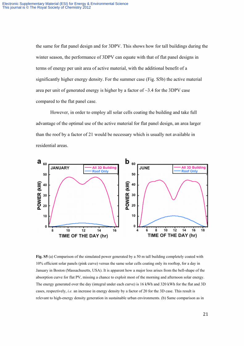
the same for flat panel design and for 3DPV. This shows how for tall buildings during the
winter season, the performance of 3DPV can equate with that of flat panel designs in
terms of energy per unit area of active material, with the additional benefit of a
significantly higher energy density. For the summer case (Fig. S5b) the active material
area per unit of generated energy is higher by a factor of ~3.4 for the 3DPV case
compared to the flat panel case.
However, in order to employ all solar cells coating the building and take full
advantage of the optimal use of the active material for flat panel design, an area larger
than the roof by a factor of 21 would be necessary which is usually not available in
residential areas.
Fig. S5 (a) Comparison of the simulated power generated by a 50 m tall building completely coated with
10% efficient solar panels (pink curve) versus the same solar cells coating only its rooftop, for a day in
January in Boston (Massachusetts, USA). It is apparent how a major loss arises from the bell-shape of the
absorption curve for flat PV, missing a chance to exploit most of the morning and afternoon solar energy.
The energy generated over the day (integral under each curve) is 16 kWh and 320 kWh for the flat and 3D
cases, respectively, i.e. an increase in energy density by a factor of 20 for the 3D case. This result is
relevant to high-energy density generation in sustainable urban environments. (b) Same comparison as in
Electronic Supplementary Material (ESI) for Energy & Environmental ScienceThis journal is © The Royal Society of Chemistry 2012

22
(a), but for a day in June in Boston. The energy generated over the day is 85 kWh and 525 kWh for the flat
and 3D case, respectively. Note that the 3D case is less season-sensitive, given the decrease in generated
energy by a factor of 5.3 between June and January for the flat case, and of only 1.65 for the 3D case.
Design of a 3D e-bike charger.
As another example of an application based on 3DPV currently, we consider the
design of a 3D charger for electric bicycles (e-bikes). E-bikes are an emerging
commodity with an anticipated growing market demand. The Electric Bikes Worldwide
Reports of 201033 estimates that 1,000,000 e-bikes will be sold in Europe in 2010, and
that sales in the U.S. will reach roughly 300,000 in 2010, doubling the number sold in
2009. We studied a number of shapes for e-bike charging towers based on PV panels
arranged in 3D, with a base area of roughly 1 m2 and a height of 4 m for all structures.
Candidate shapes were first designed using CAD software and then obtained as a
set of triangles that can be studied using our 3DPV code (Fig. S6a,b). The energy
generated over a year in Boston was calculated for all candidate shapes, using solar cells
with 17 % efficiency and 4 % reflectivity. The generated energy ranged between roughly
2–3 MWh/year for optimal shape orientations, with higher values for designs with more
“boxy” attributes. Design #4 (in Fig. S6a) achieved a maximum simulated energy
generation of 3,017 kWh/year, although design #6 – yielding a lower value of 2,525
kWh/year – could be more appealing as a prototype due to stability under different
weather and wind considerations. These figures are likely an overestimate by 20–30 %
due to the effects of weather reducing the annual insolation. The charger we are
considering can further store power generated during the day in a battery hosted in a
compartment placed at the base of the tower (Fig. S6c).
Electronic Supplementary Material (ESI) for Energy & Environmental ScienceThis journal is © The Royal Society of Chemistry 2012

23
Fig. S6 (a) Candidate shapes for an e-bike charging tower. (b) Shapes in (a) obtained as set of triangles that
can be analyzed with the 3DPV code, with energy generation of 2 – 3 MWh/year. (c) Schematics of a
prototype for an e-bike charging station with compact design and easy to integrate in the urban
environment. (d) Drawing of an e-bike charging station in the Boston Common and Public Gardens in
Boston, MA.
Assuming an ideal charging process and a typical energy consumption for e-bikes
of 10 – 15 Wh/mile,33 such tower could charge e-bikes for at least 130,000 miles/year
when weather loss are taken into account. Installation of multiple stations in urban areas
(Fig. S6d) would facilitate the deployment of e-bike technology, while using charging
station of small footprint area, indeed a key feature of 3DPV.
Electronic Supplementary Material (ESI) for Energy & Environmental ScienceThis journal is © The Royal Society of Chemistry 2012
24
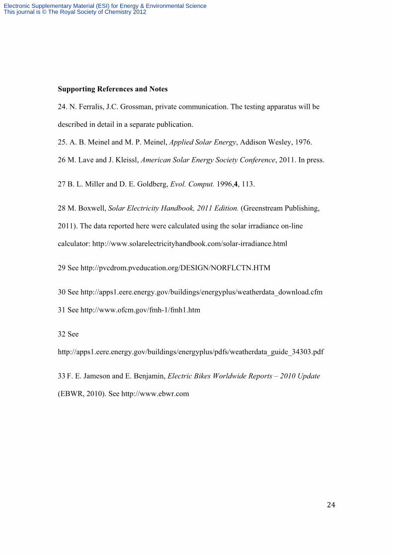
Supporting References and Notes 24. N. Ferralis, J.C. Grossman, private communication. The testing apparatus will be
described in detail in a separate publication.
25. A. B. Meinel and M. P. Meinel, Applied Solar Energy, Addison Wesley, 1976.
26 M. Lave and J. Kleissl, American Solar Energy Society Conference, 2011. In press.
27 B. L. Miller and D. E. Goldberg, Evol. Comput. 1996,4, 113.
28 M. Boxwell, Solar Electricity Handbook, 2011 Edition. (Greenstream Publishing,
2011). The data reported here were calculated using the solar irradiance on-line
calculator: http://www.solarelectricityhandbook.com/solar-irradiance.html
29 See http://pvcdrom.pveducation.org/DESIGN/NORFLCTN.HTM
30 See http://apps1.eere.energy.gov/buildings/energyplus/weatherdata_download.cfm 31 See http://www.ofcm.gov/fmh-1/fmh1.htm
32 See
http://apps1.eere.energy.gov/buildings/energyplus/pdfs/weatherdata_guide_34303.pdf 33 F. E. Jameson and E. Benjamin, Electric Bikes Worldwide Reports – 2010 Update
(EBWR, 2010). See http://www.ebwr.com
Electronic Supplementary Material (ESI) for Energy & Environmental ScienceThis journal is © The Royal Society of Chemistry 2012