Small-scale Technology Certificates Data Modelling for...
64
Small-scale Technology Certificates Data Modelling for 2013 to 2015 FINAL REPORT 11 February 2013
Transcript of Small-scale Technology Certificates Data Modelling for...

Small-scale Technology Certificates Data Modelling for 2013
to 2015
FINAL REPORT
11 February 2013

PAGE ii
SKM MMA
ABN 37 001 024 095
Level 11, 452 Flinders Street
Melbourne VIC 3000 Australia
Tel: +61 3 8668 6090
Fax: +61 3 8668 3001
Web: www.globalskm.com
COPYRIGHT: The concepts and information contained in this document are the property of Sinclair Knight Merz Pty Ltd. Use or copying of this document in whole or in part without the written permission of Sinclair Knight Merz constitutes an infringement of copyright.
LIMITATION: This report has been prepared on behalf of and for the exclusive use of Sinclair Knight Merz Pty Ltd’s Client, and is subject to and issued in connection with the provisions of the agreement between Sinclair Knight Merz and its Client. Sinclair Knight Merz accepts no liability or responsibility whatsoever for or in respect of any use of or reliance upon this report by any third party.

PAGE iii
Contents 1. ABBREVIATIONS ....................................................................................................................................................... 1
2. EXECUTIVE SUMMARY ............................................................................................................................................. 2
3. BACKGROUND ......................................................................................................................................................... 6
4. GOVERNMENT INCENTIVES ..................................................................................................................................... 10
4.1. REBATES .................................................................................................................................................................... 10 4.2. FEED-IN TARIFF............................................................................................................................................................ 13
5. METHODOLOGY ...................................................................................................................................................... 16
5.1. GENERAL METHODOLOGY .............................................................................................................................................. 16 5.2. HISTORICAL DATA SET SUPPLIED BY CER ............................................................................................................................ 16 5.3. GENERAL ASSUMPTIONS ................................................................................................................................................ 17
5.3.1. Capital cost assumptions for solar PVs .......................................................................................................... 17 5.3.2. Capital cost assumptions for solar water heaters and heat pump water heaters ......................................... 18 5.3.3. Net cost model ............................................................................................................................................... 19 5.3.4. Net cost for PV ............................................................................................................................................... 19 5.3.5. Net cost for water heaters ............................................................................................................................. 21 5.3.6. Wholesale electricity price assumptions ........................................................................................................ 21
5.4. STRUCTURAL MODEL ..................................................................................................................................................... 22 5.4.1. Overview of model ......................................................................................................................................... 22 5.4.2. DOGMMA Methodology ................................................................................................................................ 23 5.4.3. Key model assumptions ................................................................................................................................. 23
5.5. TIME SERIES MODEL ...................................................................................................................................................... 23 5.5.1. Overview ........................................................................................................................................................ 23 5.5.2. Data preparation ........................................................................................................................................... 23 5.5.3. Time series model for SGUs ........................................................................................................................... 24
5.5.3.1. Choosing the external regressor ............................................................................................................... 24 5.5.3.2. Choosing the dependent variable ............................................................................................................. 25 5.5.3.3. Limiting the amount of data points in the regression ............................................................................... 25 5.5.3.4. Choosing the level of aggregation ............................................................................................................. 28 5.5.3.5. Form of the time series model .................................................................................................................. 28
5.5.4. Time series model for water heaters ............................................................................................................. 29 5.5.4.1. Choosing the external regressor ............................................................................................................... 29 5.5.4.2. Choosing the dependent variable ............................................................................................................. 29 5.5.4.3. Choosing the level of aggregation ............................................................................................................. 30 5.5.4.4. Form of the time series model .................................................................................................................. 31
6. MODELLING RESULTS .............................................................................................................................................. 32
6.1. DOGMMA PROJECTIONS ............................................................................................................................................. 32 6.2. TIME SERIES PROJECTIONS .............................................................................................................................................. 37
6.2.1. Installed PV Capacity ..................................................................................................................................... 37 6.2.2. Water heater STC projections ........................................................................................................................ 46
6.3. CERTIFICATE PROJECTIONS FOR TIME SERIES MODEL .............................................................................................................. 48 6.3.1. Interpretation of certificate projection for time series model........................................................................ 49
6.4. CERTIFICATE PROJECTIONS FOR DOGMMA ...................................................................................................................... 51 6.5. COMBINED STC VOLUME PROJECTIONS ............................................................................................................................. 51
7. CONCLUDING REMARKS .......................................................................................................................................... 53
APPENDIX A DOGMMA MODEL ASSUMPTIONS ...................................................................................................... 54

PAGE iv
A.1 CONSTRAINTS ............................................................................................................................................................. 54 A.2 LOCAL DEMAND ........................................................................................................................................................... 54 A.3 TECHNICAL ASSUMPTIONS .............................................................................................................................................. 54 A.4 PHOTOVOLTAIC SYSTEM PARAMETERS ............................................................................................................................... 55
A.4.1 Costs .............................................................................................................................................................. 55 A.4.2 Capacity factors ............................................................................................................................................. 57
A.5 SOLAR WATER HEATER AND HEAT PUMP WATER HEATER PARAMETERS ...................................................................................... 58 A.5.1 Costs .............................................................................................................................................................. 58 A.5.2 Energy displaced ............................................................................................................................................ 58
A.6 SMALL WIND PARAMETERS ............................................................................................................................................. 58 A.6.1 Costs .............................................................................................................................................................. 58 A.6.2 Capacity factors ............................................................................................................................................. 58
A.7 MINI HYDRO .............................................................................................................................................................. 59 A.8 OTHER REVENUES ........................................................................................................................................................ 59

PAGE 1
1. Abbreviations ACT Australian Capital Territory
ARIMA Autoregressive Integrated Moving Average
CPI Consumer Price Index
CPRS Carbon Pollution Reduction Scheme
DOGMMA Distributed Generation Market Model of Australia
EPIA European Photovoltaic Industry Association
FiT Feed-in Tariff
HPWH Heat Pump Water Heaters
kW Kilowatt
kWh Kilowatt hour
LRET Large-scale Renewable Energy Target
NSW New South Wales
ORER Office of the Renewable Energy Regulator
PV Photovoltaic
PVRP Photovoltaic Rebate Program
REC Renewable Energy Certificate
RET Renewable Energy Target
SGU Small Generation Unit
SHCP Solar Home and Communities Plan
SKM MMA Sinclair Knight Merz - McLennan Magasanik Associates, the strategic
consulting group within Sinclair Knight Merz resulting from the merger with
McLennan Magasanik Associates in 2010
SRES Small-scale Renewable Energy Scheme
STC Small-scale Technology Certificate
SWH Solar Water Heaters

PAGE 2
2. Executive Summary This report has been prepared for the Clean Energy Regulator (CER) and presents SKM
MMA‟s projections of the number of Small-scale Technology Certificates (STCs) expected to
be created in the 2013, 2014 and 2015 calendar years.
Two modelling approaches were used to formulate the projections. The first approach used
SKM MMA‟s DOGMMA model, which is a structural model of distributed and embedded
generation for all of Australia. It determines the uptake of small-scale renewable
technologies based on comparing the net cost of generation against the net cost of grid
delivered power. The second approach was through the construction of a time series model,
which would determine the uptake of renewable technologies based on trends in historical
data, also having regard to the historical and projected evolution of the net cost of system
installation.
Analysis of the dataset provided by CER detailing the historical creation of all STCs by
small-scale technologies revealed that the majority of STCs were created by PV systems,
solar water heaters (SWHs) and heat pump water heaters. STC projections from small-scale
wind and hydro systems were therefore not considered in the analysis since they constitute
a small fraction of the total.
Exec Figure- 1 shows the projection of total STC creation across Australia derived from the
DOGMMA model, and also includes historical STC creation to provide some context. The
method used with the DOGMMA model was to fix the historical uptake of small-scale
technology in the model to match actual uptake, and to then adjust the annual uptake
constraints to reflect the peak uptake for each region, which occurred in 2011 for most of the
regions. This method of constraint adjustments proved to be sufficient for the purpose of
deriving sensible projections from the model.
Looking forward, DOGMMA predicts a large reduction in the number of STCs created in
2013, which is mainly driven by the cessation of the solar credits multiplier. Certificate
production is then projected to decrease slightly in 2014 and remain at a similar level in
2015.

PAGE 3
Exec Figure- 1 Total STC creation for Australia using DOGMMA
Exec Figure- 2 shows the projection of monthly PV capacity across Australia derived from
the time series model. This variable has been used to illustrate future STC trends resulting
from the time series modelling because it dominates current and future STC creation. The
solid black line on the left is the historical monthly newly installed PV capacity, and the solid
red line on the right is the projection. The green dotted line is the time series model‟s fit to
the historical PV uptake, which appears to be quite good, although it falls short of the 2011
peak. According to the time series model, the monthly PV uptake has already peaked twice
– in mid 2011 and mid 2012 - and the model is projecting decreasing PV uptake over the
next three years. The stark jumps evident in the monthly projections occur every July from
July 2014 onwards. These are primarily driven by the monthly PV net cost projection, and
reflect the annual change in the carbon price. The time series model predicts a clear
downtrend in PV uptake over the next three years in contrast to the DOGMMA model, which
predicts that STC creation and PV uptake will stabilise by 2015. This suggests that the steep
downtrend evident in the historical time series from July 2012 onwards is the dominant driver
of the projection.
0
10,000
20,000
30,000
40,000
50,000
60,000
70,000
2008 2009 2010 2011 2012 2013 2014 2015
STC
s cr
eat
ed
, th
ou
san
ds
Calendar year
Historical STC creation DOGMMA projection
PAGE 4
Exec Figure- 2 Monthly installed PV capacity for Australia using the time series model
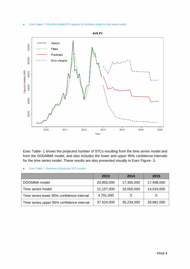
Exec Table- 1 shows the projected number of STCs resulting from the time series model and
from the DOGMMA model, and also includes the lower and upper 95% confidence intervals
for the time series model. These results are also presented visually in Exec Figure- 3.
Exec Table- 1 Summary of projected STC creation
2013 2014 2015
DOGMMA model 20,855,000 17,355,000 17,498,000
Time series model 21,157,000 16,555,000 14,019,000
Time series lower 95% confidence interval 4,791,000 0 0
Time series upper 95% confidence interval 37,524,000 35,234,000 29,681,000

PAGE 5
Exec Figure- 3 STC projections using both methodologies
The time series based STC central projection is almost 20% lower than that produced by the
DOGMMA model in 2015, although the difference in projections for 2013 and 2014 are much
lower, being 1.4% higher and 4.6% lower respectively. However, the 2015 DOGMMA
projection does lie well within the time series model‟s 95% confidence intervals. The
reduction of STCs produced in 2013 relative to 2012 is due primarily to the cessation of the
solar credits multiplier. STCs sourced from water heaters are projected to make up from 8%
to 13% of total number of certificates produced over the next three calendar years,
confirming that the dominance of PV over solar water heaters is set to continue.
In providing these projections of STC volumes over the 2013, 2014 and 2015 calendar
years, SKM MMA would like to underline the large level of uncertainty surrounding them.
This is evident from the wide range of uncertainty in the time series projections, as indicated
by the large confidence intervals in Exec Figure- 2 and Exec Figure- 3. The fundamental
source of the uncertainty underlying the PV uptake predictions is the large level of monthly
volatility in PV uptake at the state/territory level. This has been driven by a combination of
large and rapid changes in Government incentives over the last three years, and rapidly
declining capital costs of PV systems in recent times.
SKM MMA has more confidence in the STC volume projections for water heaters produced
by both models. The time series model in particular used almost seven years of market
history to make the predictions. However, these projections only form 8% to 13% of the
annual number of STCs expected to be created over the next three years, and therefore
have a much smaller weighting than the PV projections.
0
5,000
10,000
15,000
20,000
25,000
30,000
35,000
40,000
2013 2014 2015
STC
s cr
eat
ed
, th
ou
san
ds
Calendar year
DOGMMA
Time series
Time series 95% confidence intervals

PAGE 6
3. Background The Clean Energy Regulator (CER) is responsible for the implementation of the Australian
Government‟s climate change laws and programmes, one of which is the Renewable Energy
Target (RET). The specific aim of the target is to assist the government with its commitment
to achieving 20 percent of its electricity supply from renewable sources by 2020.
The RET legislation places a legal liability on wholesale purchasers of electricity to
contribute towards the government‟s yearly targets. Wholesale purchasers meet this
requirement by surrendering eligible certificates. A certificate is generally equivalent to
1MWh of renewable electricity and wholesale purchasers may create certificates through
their own power stations or purchase them from the market.
Since the start of the RET, the government has announced a change which has seen the
RET scheme split into two parts; the Small-Scale Renewable Energy Scheme (SRES) and
the Large-Scale Renewable Energy Target (LRET). These schemes became effective on the
1st January 2011.
The SRES scheme offers small-scale technology certificates (STCs) at a fixed price of $40
per certificate to purchasers of eligible solar water heaters (SWH), air source heat pump
water heaters (HPWH) and small-scale photovoltaic (PV), wind and hydro systems. There is
no cap to the number of STCs that can be created, which means that liable entities, through
whom the scheme is funded, could potentially have significant costs to cover if there is a
large uptake of these technologies.
The purpose of this report is to forecast the number of STCs that will be generated in the
calendar years of 2013, 2014 and 2015. This will assist liable entities to anticipate the extent
of their liability over the coming years.
The number of RECs and STCs created historically by each of the small-scale technologies
is shown on an annual time scale in Figure 3-1. REC creation was historically dominated by
solar water heater (SWH) installations, although this changed in 2010, where photovoltaic
systems are now making the largest contribution, and continue to contribute the greatest
proportion of STCs created.
The three stand-out trends are: (i) the large volume of SWH RECs created in 2009, which
was one factor responsible for the fall of the spot REC price at the time; (ii) the even larger
volume of photovoltaic STCs created in 2010 through to 2012; and (iii) the turning point in
STC creation, which peaked in 2011. The large increase in SWH RECs was driven by a
change in the incentives offered to home owners by means of the Solar Hot Water Rebate,
which commenced from 1 July 2009 and ended on 19 February 2010. This offered a rebate
of up to $1600 to eligible householders for installing a SWH that replaced an electric hot
water storage system.
From 2010 onwards, PV became the dominant small-scale renewable technology, and
installations grew at an exponential rate. There are a number of factors explaining the rapid
uptake of PV systems over the last three years. Firstly, the installed cost of PV systems
plummeted in 2009 and 2010. Over about one year, the cost of these systems halved. At

PAGE 7
the same time, their affordability was aided by the rising Australian dollar, and the
government incentives that were offered. Secondly, the Federal Government‟s Photovoltaic
Rebate Program (PVRP) increased from $4000 to $8000 as of November 2007, and this
was followed by the subsequent issuance of solar credits for SGUs under the expanded RET
scheme, from 9 September 2009 (superseding the PVRP). Thirdly, various state
governments introduced feed-in tariffs (FiTs). Queensland was the first, offering a net FiT of
44 c/kWh in July 2008, and WA was the last, offering a net FiT of 40c/kWh in August 2010.
The popularity of these schemes was evident in the fact that they were fully subscribed in a
short period of time, and all of the original schemes have either ceased or have since been
cut back in one way or another.
Figure 3-1 RECs/STCs created historically from small-scale technologies – Calendar years
2011 has proven to be the peak year for STC creation. This is primarily due to the solar
credits multiplier received by PV systems in that year, being 5 from January to June and
then stepping down to 3 from July to December. In addition PV capital costs were at a then
all time low due to the factors mentioned above, and there were still generous FiTs on offer
in many of the states. The other factor that would have contributed to the 2011 peak1 was
that consumers would have been better informed about the benefits of PV systems relative
to their awareness in 2010.
Even though many of the government incentives had ceased, or were reduced in 2012, this
still proved a strong year for STC creation. Factors supporting small-scale technology uptake
and STC creation in 2012 were: (i) a further 40% reduction in the installed cost of PV
systems, which have fallen to about $2,700/kW by the end of 2012, compared to about
$4,500/kW in mid 2011; (ii) the continuation of the solar credits multiplier, albeit at a lower
1 All of the factors mentioned for the 2011 peak also existed in 2010.
0
10,000
20,000
30,000
40,000
50,000
60,000
70,000
2001 2002 2003 2004 2005 2006 2007 2008 2009 2010 2011 2012
Nu
mb
er
of
REC
s/ST
Cs
cre
ate
d (
'00
0s)
Calendar Year
Hydro
Wind
SWH
PV

PAGE 8
level; (iii) the continuation of FiTs in some of the states, especially Queensland, where 2012
STC creation was greatest, and South Australia; and (iv) the trend towards larger system
sizes.
The proportion of different PV system sizes being installed in the market is shown in Figure
3-2. The graph shows an increasing proportion of installation of system sizes of 1.5kW or
less between 2008 and 2009, whereas from 2010 onwards there is a rapid decline in the
installation of small PV systems. This change in trend from 2010 onwards is mirrored by an
increase in the proportion of system sizes between 1.5kW and 3kW, and a gradually
increasing proportion of sizes 3kW to 5kW and higher. In 2011, the installation proportion of
1.5kW to 3kW systems peaked, and in 2012 the installation proportions of systems greater
than 3kW continues to increase.
Figure 3-2 Proportion of system sizes installed
The sharp increase in the proportion of 1.5kW system between 2008 and 2009 is likely
reflective of the introduction of the 5x solar credits multiplier in 2009. The declining
proportion of smaller system sizes since then is assumed to have occurred for a number of
reasons:
The solar credits multiplier is likely to have increased the affordability of larger systems, since
the multiplier still applies to the first 1.5kW;
Uncertainty surrounding the future carbon price and its impact on retail electricity prices is
likely to have encouraged uptake of larger systems to offset the expected increase in
electricity charges through avoided costs of future electricity consumption; and
0%
10%
20%
30%
40%
50%
60%
70%
80%
90%
2003 2004 2005 2006 2007 2008 2009 2010 2011 2012
% o
f to
tal i
nst
alla
tio
ns
Calendar year
<=1.5 kW 1.5kW to 3kW 3kW to 5kW >5kW

PAGE 9
Changes in FiT schemes in some states from a gross scheme to a net scheme, stimulating
demand for larger systems to generate more electricity for export to the grid.
The rapid rise of retail electricity prices over the last five years has encouraged consumers to
buy larger systems in order to generate enough electricity to either eliminate or minimise their
electricity bill.
The remainder of this report has been set out as follows:
Government incentives: A discussion of federal and state incentives and FiTs that may
influence a users‟ decision to take up small-scale renewable technologies, and which form
underlying assumptions for net cost calculations in the modelling
Methodology: Presents the key modelling assumptions and the methodologies underlying both
SKM MMA‟s DOGMMA model and the time series model utilised in this assignment; and
Modelling results: Presents the results of the modelling using both models and then translates
these into projected STC volumes for the 2012, 2013 and 2014 calendar years.
PAGE 10
4. Government incentives The number of STCs that will be generated in 2013, 2014 and 2015 is dependent on uptake
of eligible technologies by households and business which is in turn influenced by financial
incentives such as federal and state rebates and the state-based FiT schemes. Many of
these incentives have now ceased as they have achieved their objective, which was to
stimulate a sizeable level of small-scale renewable technology uptake for both residential
and commercial sectors.
Additional factors impacting the perceived cost or net cost of renewable technologies
including the avoided cost of electricity consumed are discussed in Section 5.3.3.
4.1. Rebates
In order to address the high up-front cost of installation and to encourage households and
businesses to adopt renewable technologies, Australian governments had initiated a number
of Federal and State rebates. This section provides an overview of historical rebates
pertaining to solar PVs, SWHs and HPWHs as well as the few incentives for installers that
still remain active.
The Australian Government through the Department of Climate Change and Energy
Efficiency launched the Photovoltaic Rebate Program (PVRP) in 2000 where individuals and
households, regardless of income received a rebate of $4,000 for installing solar PVs. In
October 2007 the program was replaced by the Solar Home and Communities Plan (SHCP).
This plan assisted with the installation of more than 100,000 systems and since then it has
been replaced by the Solar Credits program.
In addition to the solar PV rebates, the Australian Government also provided support to
individuals and households through the solar hot water rebate program. The program initially
offered $1,600 and $1,000 in rebates for solar water heaters and heat pump water heaters
respectively, and these were then reduced under the Renewable Energy Bonus Scheme to
$1000 and $600 respectively from 20 February 2010.
In addition to the federal rebates, a number of state initiatives also provided assistance.
Table 4-1 provides a summary of the now historical Federal rebates; and
Table 4-2 provides a summary of solar water heater and heat pump water heater rebates by state.

PAGE 11
Table 4-1 Historical rebates offered by the Federal Government
Historical
System Information Description
Solar PVs
Name: Photovoltaic Rebate Program (PVRP)
Valid: From 2000 to October 2007
A rebate of $4,000 and not subjected to a means test.
Name: Solar Homes and Communities Plan (SHCP)
Valid: November 2007 to 6 July 2009
The SHCP started out as the PVRP and provided support to households through a solar panel rebate. For the greater part of the plan, it was subjected to a means test of $100,000 or less. The SHCP offered the following rebate:
For new systems - Up to $8,000 ($8 per watt up to one kilowatt); and
For extensions to old systems - Up to $5,000 ($5 per watt up to one kilowatt)
SWH Name: Solar hot water rebate program
Valid: Until 19 February 2010
A rebate of $1,600 and not subjected to a means test.
HPWH Name: Solar hot water rebate program
Valid: Until 19 February 2010
A rebate of $1,000 and not subjected to a means test.
SWH Name: Renewable Energy Bonus Scheme - Solar hot water rebate program
Valid: From 20 February 2010 to 30 June 2012
A rebate of $1,000 and not subjected to a means test.
From 1 November 2011, only systems that are able to generate 20 or more STCs were eligible for the rebate.
HPWH Name: Renewable energy bonus scheme - Solar hot water rebate program
Valid: From 20 February 2010 to 30 June 2012
A rebate of $600 and not subjected to a means test. From 1 November 2011, only systems that are able to generate 20 or more STCs were eligible for the rebate.
Solar PVs
Name: Solar credits
Valid: From 9 June 2009
to 31 December 2012
This scheme replaced the SHCP and the extent of the rebate was dependent on the size of the system and the date of installation.
A multiplier was applied to the first 1.5kW of eligible systems where the balance received no multiplier. The multiplier was gradually stepped down to reflect technological advances. From 9 June 2009 until 30 June 2011 the multiplier was 5. From 1 July 2011 until 30 June 2012 the multiplier was 3. From 1 July 2012 until 31 December 2012 the multiplier was 2, and from 1 January 2013 onwards it was 1.

PAGE 12
Table 4-2 Summary of solar water heater and heat pump water heater rebates by State governments
Historical
State Information Description
New South Wales Name: NSW hot water system rebate
Valid: From October 2007 to 30 June 2011
A rebate of $300 for a solar or heat pump hot water system
Northern Territory Name: Solar hot water retrofit rebate
Valid: From 1 July 2009 to 30 June 2010
Northern Territory households may have been eligible for a Solar Hot Water Retrofit Rebate of up to $1,000 to help with the costs of installing a solar hot water system.
Queensland Name: Queensland government solar hot water rebate
Valid: From 13 April 2010 to 22 June 2012
A $600 rebate for the installation of a solar or heat pump hot water system; or
A $1000 rebate for pensioners and low income earners who installed a solar or heat pump hot water system.
Tasmania Name: Solar and Heat Pump Hot Water Rebate Scheme
Valid: 1 July 2007 to 31 December 2011 (solar hot water systems)
Valid: 1 November 2008 to 31 December 2011 (heat pump water systems)
This scheme offered Hobart ratepayers a $500
incentive to install a solar or heat pump hot water
system into their homes.
Current
Victoria Name: Victorian solar hot water rebate
Valid: From July 2008 until current
A rebate from $400 to $1600 and from $300 to $1500 for regional Victoria and metropolitan Melbourne respectively for both solar water heaters and heat pump water heaters.
Australian Capital Territory
Name: HEAT Energy Audit
Valid: From December 2004 to current
A $500 rebate is available for expenditure of $2,000 or more on the priority recommendations in the ACT Energy Wise audit report - which can include installing solar or heat pump water heating.
Western Australia Name: Solar water heater subsidy
Valid: From July 2010 to
30 June 2013
A rebate of $500 for natural gas-boosted solar or heat pump water heaters; and
A rebate of $700 for bottled LP gas-boosted solar or heat pump water heaters used in areas without reticulated gas.
South Australia Name: South Australian Government‟s Solar Hot Water Rebate scheme
Valid: From 1 July 2008 to current
A rebate of $500 for a new solar or electric heat pump water heater system. In order to be considered for this rebate, applicants must an Australian government concession card.
Where a range of possible rebates were available, SKM MMA generally assumed a rebate at
the lower range of the scale. No rebate was assumed to apply for a typical SWH or HPWH
installer in South Australia since the rebates in that state are only available to low-income

PAGE 13
earners. Similarly, no rebate was assumed to apply in the ACT since solar and heat pump
water heating have a fairly low priority on the list of eligible activities. Funding for the
Victorian scheme is open-ended for the moment and its continuation depends on its
inclusion in the State‟s budget. Given the cessation of similar schemes in the other states,
SKM MMA assumed that funding for the Victorian scheme would end on 30 June 2014.
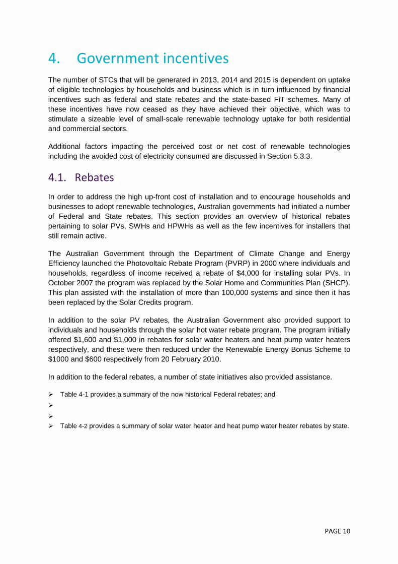
4.2. Feed-in tariff
Feed-in tariffs in Australia for small-scale renewable energy generation are offered by the
state governments. Table 4-3 presents a detailed summary of the FiTs offered by state.

PAGE 14
Table 4-3 Summary of feed-in tariffs
State/Territory Current arrangement SKM MMA assumptions for 2013-2015 Previous arrangements
Victoria Net FiT of 8c/kWh, commencing from 1 October 2012.
Net FiT of 8c/kWh remaining flat in nominal terms over modelling horizon.
Net FiT of 60c/kWh commenced in November 2009 and ended on 30 September 2011. Net transitional FiT of 25c/kWh plus retailer contribution up to 8c/kWh replaced this from 1 January 2012, with the rate available for 5 years. This offer ended on 30 September 2012.
New South Wales Net FiTs offered by retailers range from 0c/kWh to 7.7c/kWh2.
Net FiT of 7.7c/kWh remaining flat in nominal terms over modelling horizon.
Gross FiT of 60c/kWh commenced in January 2010. FiT was reduced to 20c/kWh on 27 October 2010 and has since closed to new applicants as of 28 April 2011.
Queensland
Net FiT of 8c/kWh for systems up to 5kW in size, plus an additional 6c/kWh to 8c/kWh retailer contribution, commencing 9 July 2012.
Net FiT of 15c/kWh remaining flat in nominal terms over modelling horizon.
Net FiT of 44c/kWh commenced in July 2008. From 8 June 2011, only systems up to 5kW in size were eligible.
Northern Territory
Gross 1-for-1 FiT, where consumer is paid for all electricity generated at their consumption tariff.
Gross FiT at assumed NT retail prices for domestic and commercial customers.
Customers on the Alice Springs grid received 51.28 c/kWh, capped at $5 per day, for all PV-generated electricity through the Alice City Solar Program. This program is now closed to new customers.
Australian Capital Territory
Net 1-for-1 FiT, where consumer is paid for electricity exported to the grid at their consumption tariff.
Net FiT at assumed ACT retail prices for domestic and commercial customers.
Gross feed-in tariff of 50.5 c/kWh commenced in March 2009. The scheme was revised in April 2010, and the feed-in tariff was reduced to 45.7 c/kWh. This revised scheme ended on 31 May 2011.
On 1 July 2011, small scale units were allowed to receive credits under the medium scale program. This
2 7.7c/kWh is the minimum payment for solar FiTs recommended by IPART as fair and reasonable for electricity generated by small-scale solar PV units in NSW for 2012-13. The actual recommendation was for a rate range of 7.7 c/kWh to 12.9 c/kWh.
PAGE 15
State/Territory Current arrangement SKM MMA assumptions for 2013-2015 Previous arrangements
scheme commenced on 12 July 2011 for a rate of 30.16/kWh.
Due to overwhelming demand, the available cap was quickly taken up and the scheme closed the day after on 13 July 2011.
Western Australia
Synergy customers will be paid 8c/kWh for energy exported to the grid for systems up to 5kW in size. From 1 July 2012, Horizon Power customers are paid a minimum buyback rate of 10c/kWh and a maximum rate of 50c/kWh depending on their location, for systems up to 30kW in size.
8c/kWh for Synergy service area and 10c/kWh for Horizon Power service area as the model is not sufficiently disaggregated to model Horizon Power service area in greater detail.
Net feed-in tariff of 40 c/kWh commenced from August 2010. The tariff was cut to 20c/kWh for applications received from 1 July 2011. As of August 2011 the scheme was closed to new applicants. From August 2011 onwards, all Synergy and Horizon Power customers received 8c/kWh for energy exported to the grid.
South Australia
Net FiT of 16c/kWh plus electricity retailer contribution as follows:
27 Jan 2012 to 30 Jun 2012 – 7.1c/kWh
then to 30 Jun 2013 – 9.8c/kWh
then to 30 Jun 2014 – 11.2c/kWh
Net FiT including retailer contribution, and from 1 July 2014 retailer contribution escalates at CPI until 30 Sep 2016, when FiT ends.
Net feed-in tariff of 44 c/kWh commenced in July 2008. The scheme was revised on 1 October 2011, and the feed-in tariff was reduced to 16 c/kWh for households joining after 31 October 2011.
Tasmania Net 1-for-1 FiT, where consumer is paid for electricity exported to the grid at their consumption tariff.
Net FiT at assumed Tasmanian retail prices for domestic and commercial customers.
As per current arrangement
PAGE 16
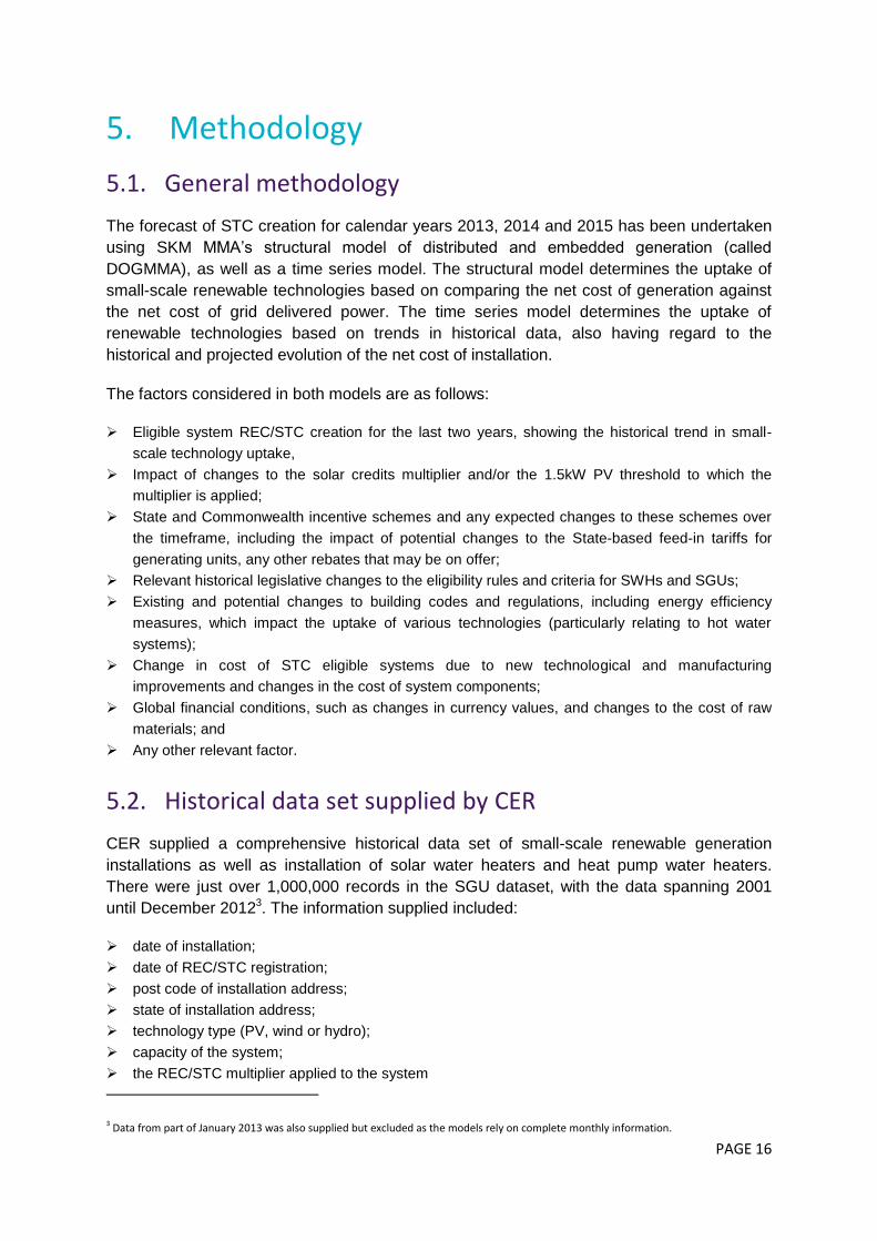
5. Methodology
5.1. General methodology
The forecast of STC creation for calendar years 2013, 2014 and 2015 has been undertaken
using SKM MMA‟s structural model of distributed and embedded generation (called
DOGMMA), as well as a time series model. The structural model determines the uptake of
small-scale renewable technologies based on comparing the net cost of generation against
the net cost of grid delivered power. The time series model determines the uptake of
renewable technologies based on trends in historical data, also having regard to the
historical and projected evolution of the net cost of installation.
The factors considered in both models are as follows:
Eligible system REC/STC creation for the last two years, showing the historical trend in small-
scale technology uptake,
Impact of changes to the solar credits multiplier and/or the 1.5kW PV threshold to which the
multiplier is applied;
State and Commonwealth incentive schemes and any expected changes to these schemes over
the timeframe, including the impact of potential changes to the State-based feed-in tariffs for
generating units, any other rebates that may be on offer;
Relevant historical legislative changes to the eligibility rules and criteria for SWHs and SGUs;
Existing and potential changes to building codes and regulations, including energy efficiency
measures, which impact the uptake of various technologies (particularly relating to hot water
systems);
Change in cost of STC eligible systems due to new technological and manufacturing
improvements and changes in the cost of system components;
Global financial conditions, such as changes in currency values, and changes to the cost of raw
materials; and
Any other relevant factor.
5.2. Historical data set supplied by CER
CER supplied a comprehensive historical data set of small-scale renewable generation
installations as well as installation of solar water heaters and heat pump water heaters.
There were just over 1,000,000 records in the SGU dataset, with the data spanning 2001
until December 20123. The information supplied included:
date of installation;
date of REC/STC registration;
post code of installation address;
state of installation address;
technology type (PV, wind or hydro);
capacity of the system;
the REC/STC multiplier applied to the system
3 Data from part of January 2013 was also supplied but excluded as the models rely on complete monthly information.

PAGE 17
number of RECs/STCs registered by the system;
number of RECs/STCs that passed/failed the validation audit
The data showed that the number of STCs created by small-scale PV systems was
significantly greater than STCs produced by small-scale wind and hydro. As such, certificate
projections for small-scale wind and hydro were not carried out as their contribution to the
total would be negligible.
The dataset comprising SWHs and HPWHs contained over 808,000 records covering the
same time span as the SGU dataset. Supplied information included:
date of installation;
date of REC/STC registration;
post code of installation address;
state of installation address;
technology type (SWH or HPWH);
number of RECs/STCs registered by the system; and
whether the system capacity was over 700 litres.
These data were primarily used to construct the historical time series data, thus enabling the
utilisation of time series analysis. The SGU capacity data were also summarised in a form to
allow comparison with the DOGMMA model.
5.3. General assumptions
The following section presents our key modelling assumptions. Capital cost assumptions for
2013 are based on market research conducted by SKM MMA for a range of suppliers across
Australia, and represents an average cost per kW including installation and before any
Government rebates or credits.
5.3.1. Capital cost assumptions for solar PVs
Figure 5-1 shows the assumed capital costs for an installed PV system in nominal dollars.
This was converted into real dollars for the modelling using historical CPI and assuming CPI
of 2.5% p.a. for projections. The most notable feature of the graph is the significant reduction
in the capital cost which occurred during the 2009/10 financial year and a further significant
reduction during the 2011/2012 financial year. Capital cost is assumed to further decline at a
rate according to EPIA‟s latest projection, which averages at about 2.6% per annum in real
terms over the next decade4. The DOGMMA model also incorporates a decreasing capital
cost as the system size increases, reflecting certain available economies of scale, which
have been confirmed from the market research undertaken for this study. These cost
assumptions are further described in Appendix A.
4 Source: Connecting the Sun: Solar photovoltaics on the road to large-scale grid integration, European Photovoltaic Industry Association, September 2012, p.18.

PAGE 18
Figure 5-1 Capital costs assumed for solar PVs – ($ nominal/kW)
Source: SKM MMA market analysis with historical prices based on AECOM report to Industry and Investment NSW, Solar
Bonus Scheme: Forecast NSW PV Capacity and Tariff Payments, October 2010
5.3.2. Capital cost assumptions for solar water heaters and heat pump water heaters
Figure 5-2 shows the assumed capital costs for solar water heaters and heat pump water
heaters in nominal dollars for a typical domestic unit5. Capital cost is assumed to remain
constant in real terms between 2013 and 2015 which is reflective of the relatively mature
technologies compared with PV systems.
5 With a capacity of 315 litres
$0
$2,000
$4,000
$6,000
$8,000
$10,000
$12,000
$14,000
$16,000
$18,000
2002 2003 2004 2005 2006 2007 2008 2009 2010 2011 2012 2013 2014 2015
$/k
W (
no
min
al)
Financial year ending June
Historical Forecast

PAGE 19
Figure 5-2 Capital costs assumed for typical domestic SWH and HPWH unit – (nominal dollars)
5.3.3. Net cost model
The net cost for SGUs, SWHs and HPWHs is a key variable in explaining the uptake of
these systems for the time series analysis, and was central to the uptake forecasts using the
time series model. It also drives the output of the DOGMMA model, which is a forward
looking optimisation model that seeks to minimise total energy supply costs from the
consumer‟s viewpoint.
The net cost is defined as follows:
Sum of capital cost including installation
Less
o Value of any available government rebates
o Revenue from the sale of RECs6 and/or STCs, including the effect of the solar credits
multiplier
o Net present value of future feed-in tariff payments and/or retailer payments for export to
the grid
o Net present value of the avoided cost of electricity
5.3.4. Net cost for PV
Figure 5-3 shows the net cost for a 1.5 kW PV system installed in NSW. Movements in the
net cost are representative of trends in all Australian States and Territories, although these
6 Prior to 2011
$4,000
$4,200
$4,400
$4,600
$4,800
$5,000
$5,200
$5,400
2002 2003 2004 2005 2006 2007 2008 2009 2010 2011 2012 2013 2014 2015
$/k
W (
no
min
al)
Financial year ending June
SWH HPWH
Historical Forecast

PAGE 20
may occur at different time periods as they are dependent on the timing of the various
schemes and rebates applicable to PV systems.
Figure 5-3 Net cost for typical PV system installed in NSW
The net cost represents the cost of a 1.5kW system, however it is based on a net cost per
kW which incorporates the increasing trend of systems installed with size greater than 1.5kW
(see Figure 3-2). As such, net cost assumptions including the solar credits multiplier and
estimated FiT revenue have been adjusted to reflect the proportion of systems greater than
1.5kW.
The historical net cost reduces gradually from 2001 until 2007, and then there is a significant
drop in the net cost in late 2007, which corresponds to the increase in the Federal
government‟s PVRP rebate from $4,000 to $8,000. The sudden increase in net cost in mid
2009 represents the abolition of the PVRP rebate and its replacement by the solar credits
multiplier. This is followed by another steep decline in the net cost, which reflects the rapid
reduction in PV capital costs, and in the NSW context it also reflects the introduction of the
gross feed-in tariff. The subsequent increase in late 2010 corresponds to the reduction in the
NSW gross feed-in tariff from 60 c/kWh to 20c/kWh, and the subsequent closing of the
scheme to new applicants on 28 April 2011. This is followed by a line segment with a mildly
negative slope which turns into a long-term downtrend in net cost. The flattening out of the
slope is significant because beyond 2015 the slope turns positive again indicating a shallow
long-term uptrend in net cost. The two drivers underlying the decreasing long term cost trend
are the decreasing capital cost (see Figure 5-1) and the increasing avoided cost of
electricity, including the impact of the carbon price.
-$10,000
-$5,000
$0
$5,000
$10,000
$15,000
$20,000
$25,000
$30,000
Ne
t co
st (
$2
01
2)

PAGE 21
5.3.5. Net cost for water heaters
Figure 5-4 shows the net cost for a typical domestic SWH system installed in NSW, which is
representative of the net cost trends in all Australian States and Territories. The historical net
cost reduces gradually from 2001 until 2007, and then there is a significant drop in the net
cost in late 2007, which corresponds to the introduction of the Federal government‟s solar
hot water rebate program. The increase in the net cost in early 2010 corresponds to the
reduction in the Federal government‟s SWH rebate from $1,600 to $1,000. From 2010 to
early 2012, the net cost continues to exhibit an upward trend, which is reflective of the
assumed flat projected capital cost and the cessation of the state-based rebate. In March
2012 there is a step up in the net cost of $1,000, which reflects the cessation of the Federal
Renewable Energy Bonus Scheme. The downtrend that commences in early 2012 persists
for the long term, with the main factor for the downtrend being the increasing avoided cost of
electricity, including the impact of the carbon price.
Figure 5-4 Net cost for typical domestic SWH installed in NSW
5.3.6. Wholesale electricity price assumptions
SKM MMA‟s base case wholesale electricity prices were used as the basis for estimating
retail electricity prices, which in turn were used in calculating future electricity savings and/or
revenues for SGUs, SWHs and HPWHs. The base case assumes medium economic
demand growth, which is about 1% p.a. lower than it was one year ago, reflecting the
general slow-down of electricity demand growth in Australia, and includes the impact of
carbon pricing. The choice of carbon price scenario can potentially have a large impact on
future electricity wholesale prices. SKM MMA‟s carbon price assumption, shown in Figure
5-5, was based on the current weakness in the European carbon price, and assumes that
-$1,000
$-
$1,000
$2,000
$3,000
$4,000
$5,000
Ne
t co
st (
$2
01
2)
PAGE 22
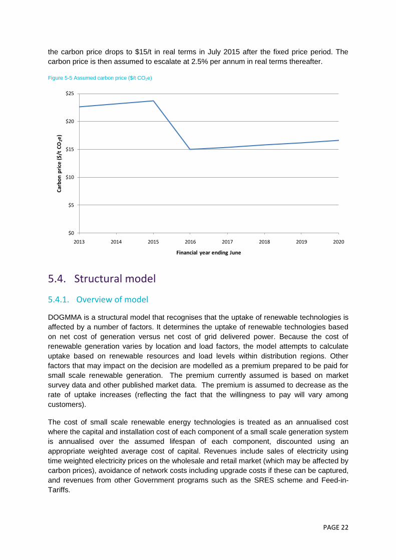
the carbon price drops to $15/t in real terms in July 2015 after the fixed price period. The
carbon price is then assumed to escalate at 2.5% per annum in real terms thereafter.
Figure 5-5 Assumed carbon price ($/t CO2e)
5.4. Structural model
5.4.1. Overview of model
DOGMMA is a structural model that recognises that the uptake of renewable technologies is
affected by a number of factors. It determines the uptake of renewable technologies based
on net cost of generation versus net cost of grid delivered power. Because the cost of
renewable generation varies by location and load factors, the model attempts to calculate
uptake based on renewable resources and load levels within distribution regions. Other
factors that may impact on the decision are modelled as a premium prepared to be paid for
small scale renewable generation. The premium currently assumed is based on market
survey data and other published market data. The premium is assumed to decrease as the
rate of uptake increases (reflecting the fact that the willingness to pay will vary among
customers).
The cost of small scale renewable energy technologies is treated as an annualised cost
where the capital and installation cost of each component of a small scale generation system
is annualised over the assumed lifespan of each component, discounted using an
appropriate weighted average cost of capital. Revenues include sales of electricity using
time weighted electricity prices on the wholesale and retail market (which may be affected by
carbon prices), avoidance of network costs including upgrade costs if these can be captured,
and revenues from other Government programs such as the SRES scheme and Feed-in-
Tariffs.
$0
$5
$10
$15
$20
$25
2013 2014 2015 2016 2017 2018 2019 2020
Car
bo
n p
rice
($
/t C
O2e
)
Financial year ending June

PAGE 23
5.4.2. DOGMMA Methodology
In the past, the DOGMMA model was calibrated to reasonably fit the historical time series
data by state on a financial year basis. The parameters that were adjusted to facilitate the
calibration included constraints on the uptake by state of any particular technology type and
size (domestic or commercial) and also the assumed net export of electricity into the grid by
state, technology type and size. Adjusting these parameters in the past proved to be enough
to obtain a reasonable fit for all states. However, the combination of large changes to
government incentives and large changes in PV capital costs over the last two years in
particular, has meant that calibration of the DOGMMA model using the above method has
not been possible. The reason for this is that DOGMMA optimises small-scale technology
uptake using perfect foresight, which is a limitation of the modelling technique, and under
perfect foresight, the most optimal solution is to build as much small-scale capacity as
possible at the front-end of the modelling time frame in order to maximise the benefit of the
FiTs, which have now ceased.
In place of this method, the historical uptake of small-scale technology has now been fixed in
the DOGMMA model to match actual uptake, and the annual uptake constraints have been
adjusted to reflect peak uptake for each region, which occurred in 2011 for most of the
regions. Since it is expected that government incentives for this sector will slowly reduce
over time, and there will no longer be wild swings in the parameters of these incentives,
calibration of DOGMMA to uptake post 2012 should be possible in future work. In the
meantime, the constraint adjustments made in this round of modelling have sufficed for the
purpose of deriving sensible projections from the model.
5.4.3. Key model assumptions
The key model assumptions for the DOGMMA model are provided in Appendix A. These
include assumptions about SGU uptake constraints, SGU capital cost assumptions and
other technical assumptions.
5.5. Time series model
5.5.1. Overview
A time series is a sequence of data points measured at different points in time, and its
analysis comprises methods for extracting meaningful characteristics of the data (e.g. trend,
seasonality, autocorrelation). Forecasting using time series techniques involves predicting
future events based on a model of the data built upon known past events. Unlike other types
of statistical regression analysis, a time series model accounts for the natural order of the
observations and will reflect the fact that observations close together in time will generally be
more closely related than observations further apart.
5.5.2. Data preparation
As detailed in Section 5.2, ORER provided SKM MMA with data on all SGU and water
heater installations for Australia. For the purposes of the time series modelling, the data was
processed and aggregated into monthly steps to create time series by technology for each

PAGE 24
state. It was important to separate the time series by state since each state has its own feed-
in tariff arrangement, which is a critical component of the economics of installing an SGU. In
the case of SWHs and HPWHs, the assumed STC creation cut-off point distinguishing a
commercial system from a domestic system was retained from the last modelling study, as
this point has now settled down. The modelling for SWHs and HPWHs were not done on
state level because it was found that this increased the error in the predictions.
All time series modelling was conducted in R, a programming language and software
environment for statistical computing. Among many other features, R provides a wide variety
of time-series analysis algorithms, and its programming language allows users to add
additional functionality as needed.
5.5.3. Time series model for SGUs
Figure 5-6 shows the time series corresponding to the total number of RECs/STCs
registered per month for the different SGU technologies. As previously noted, the
RECs/STCs are largely dominated by PVs, with RECs/STCs registered by small wind and
small hydro projects being several orders of magnitude smaller than PVs. The number of
STCs generated by small wind and small hydro are expected to continue as insignificant
relative to those generated by PVs, and therefore are not included in the modelling.
Figure 5-6 Number of RECs registered for SGUs
5.5.3.1. Choosing the external regressor
In previous analysis, it has been shown that there has been an inverse relationship between
the uptake of PV technology and its net cost. In order to validate this assumption in light of
0
1,000,000
2,000,000
3,000,000
4,000,000
5,000,000
6,000,000
7,000,000
8,000,000
9,000,000
10,000,000
Jan
-01
Jul-
01
Jan
-02
Jul-
02
Jan
-03
Jul-
03
Jan
-04
Jul-
04
Jan
-05
Jul-
05
Jan
-06
Jul-
06
Jan
-07
Jul-
07
Jan
-08
Jul-
08
Jan
-09
Jul-
09
Jan
-10
Jul-
10
Jan
-11
Jul-
11
Jan
-12
Jul-
12
Nu
mb
er
of
REC
s/ST
Cs
Year
Wind PV Hydro
PAGE 25
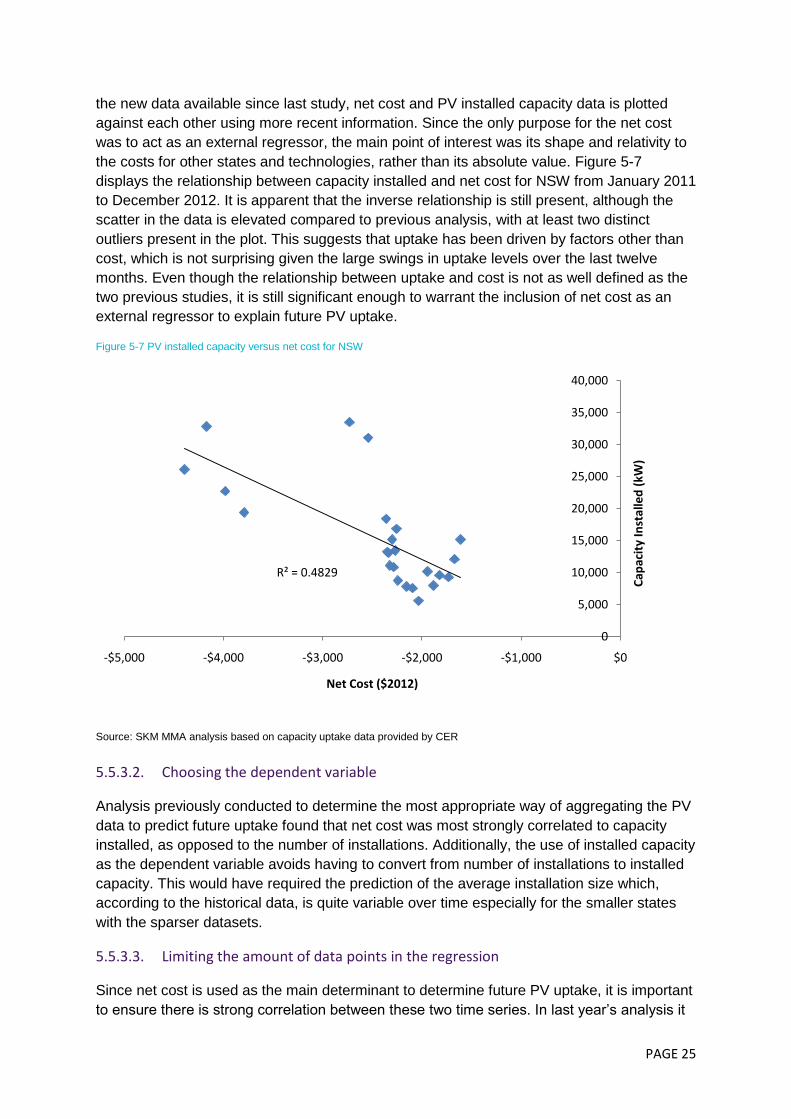
the new data available since last study, net cost and PV installed capacity data is plotted
against each other using more recent information. Since the only purpose for the net cost
was to act as an external regressor, the main point of interest was its shape and relativity to
the costs for other states and technologies, rather than its absolute value. Figure 5-7
displays the relationship between capacity installed and net cost for NSW from January 2011
to December 2012. It is apparent that the inverse relationship is still present, although the
scatter in the data is elevated compared to previous analysis, with at least two distinct
outliers present in the plot. This suggests that uptake has been driven by factors other than
cost, which is not surprising given the large swings in uptake levels over the last twelve
months. Even though the relationship between uptake and cost is not as well defined as the
two previous studies, it is still significant enough to warrant the inclusion of net cost as an
external regressor to explain future PV uptake.
Figure 5-7 PV installed capacity versus net cost for NSW
Source: SKM MMA analysis based on capacity uptake data provided by CER
5.5.3.2. Choosing the dependent variable
Analysis previously conducted to determine the most appropriate way of aggregating the PV
data to predict future uptake found that net cost was most strongly correlated to capacity
installed, as opposed to the number of installations. Additionally, the use of installed capacity
as the dependent variable avoids having to convert from number of installations to installed
capacity. This would have required the prediction of the average installation size which,
according to the historical data, is quite variable over time especially for the smaller states
with the sparser datasets.
5.5.3.3. Limiting the amount of data points in the regression
Since net cost is used as the main determinant to determine future PV uptake, it is important
to ensure there is strong correlation between these two time series. In last year‟s analysis it
R² = 0.4829
0
5,000
10,000
15,000
20,000
25,000
30,000
35,000
40,000
-$5,000 -$4,000 -$3,000 -$2,000 -$1,000 $0
Cap
acit
y In
stal
led
(kW
)
Net Cost ($2012)

PAGE 26
was established that the correlation between the net cost and the capacity installed between
July 2009 and October 2011 was quite poor for each state. With the additional data now
available up to December 2012, SKM MMA has re-examined the relationship between PV
capacity installed and its net cost through the correlation coefficient. Figure 5-8 shows the
correlation between net cost and capacity installed between July 2009 and December 2012.
It is evident that the correlation for each state between the two datasets is still quite poor,
with ACT‟s correlation being positive. It is however worthwhile noting that there has been an
improvement in correlation compared to the previous study.
Figure 5-8 Correlation between net cost and capacity installed, July 2009 - December 2012
For all states the main factor explaining the breakdown in correlation is the unexpected
announcement of a change in the initially anticipated reduction to the solar credits multiplier.
Originally the multiplier was planned to decrease from 5 to 4 in July 2011, however the
multiplier was reduced to 3 from July 2011. The data indicates that this has resulted in some
„rushed‟ buying of PV systems to take advantage of the higher multiplier before the
scheduled reduction in June 2011. Similar behaviour, although not on as large a scale,
occurred in the lead up to the July 2012 reduction of the solar credits multiplier from 3 to 2,
although in this case it was known that the reduction would be happening from 12 months
previously. Thus, it appears that the element of surprise does not explain the „rushed
buying‟, but rather that consumers put off the purchase decision to within a few months of
the cut-off. Another factor which would have made a smaller contribution to the spike in
uptake was the sudden announcement on June 25, 2012 by the Queensland government
that it would cut its feed-in-tariff from 44 cents per kilowatt to just 8 cents per kilowatt from
July 10 2012.
The subsequent low level of correlation across a number of states between net cost and
uptake compromised the predictive value of the net cost as the external regressor. SKM
MMA used the following approach to address this issue:
It was assumed that the anomalously high demand leading up to July 2011 and July
2012 was driven by impending changes to the Solar Credits multiplier and the state
feed-in tariffs, which created an atmosphere of „rushed buying‟, where consumers
made the decision to take up PV based on the fear of missing out on the maximum
ACT NSW NT QLD SA TAS VIC WA
Correlation 0.38 -0.31 -0.61 -0.58 -0.25 -0.76 -0.61 -0.80
-1.00
-0.80
-0.60
-0.40
-0.20
0.00
0.20
0.40
0.60
Co
rre
lati
on

PAGE 27
available subsidy. During this time, the relationship between uptake and net cost
temporarily broke down, but now that the rushed buying has ceased, it should be
valid again;
The rushed buying will not be repeated in the forecast period because there is no
trigger for it since the best subsidies that were on offer have now ceased;
The time frame for performing the regression characterising the relationship between
uptake and net cost has been limited for each state. The starting date is from July
2009, which corresponds with the introduction of the Solar Credits multiplier, but the
end date is based on the time frame of the rushed buying, which is different for each
state. These end dates are tabulated in Table 5-1 and were chosen to maximise the
correlation coefficient between the uptake and net cost time series.
Table 5-1 End dates for regression analysis
State Regression end dates
ACT May 2010
NSW September 2010
NT December 2010
QLD June 2010
SA June 2010
TAS December 2012
VIC May 2010
WA June 2010
The resulting correlations after limiting the end dates for regression are shown in Figure 5-9.
Figure 5-9 Correlation of net cost and installed capacity of PV with limited regression
ACT NSW NT QLD SA TAS VIC WA
Correlation -0.93 -0.83 -0.84 -0.97 -0.88 -0.76 -0.76 -0.92
-1.20
-1.00
-0.80
-0.60
-0.40
-0.20
0.00
Co
rre
lati
on

PAGE 28
5.5.3.4. Choosing the level of aggregation
The previous two studies confirmed that using separate models for small and large PV
systems (below 1.5kW or above 1.5kW) increases the variance of the respective time series
and consequently the prediction error. While data was aggregated to reflect an average
system size of 1.5kW, the average net cost is reflective of a changing trend towards a
greater proportion of installed systems greater than 1.5kW. The predicted installed capacity
was thus adjusted by the assumed proportion of system sizes when allocating installed
capacity to the relevant solar credits multiplier.
5.5.3.5. Form of the time series model
The time series at the state level were clearly non-stationary, showing both a changing mean
and changing variance over time (technically known as heteroskedasticity). However, the
logarithm of the original time series was found to be stationary after the trend was removed.
Analysing the logarithm of the time series revealed that it had no significant level of
seasonality, and thus the data lent itself nicely to an ARIMA model accompanied with an
external regressor.
Figure 5-10 Historical PV net cost by state
In summary, the time series analysis of the data for the SGUs was carried out by fitting
univariate ARIMA models to the logarithm of the monthly PV installed capacity by state with
the use of the net cost in each state as an external regressor. The historical PV net cost for
small systems are is shown in Figure 5-10, and appears to be reducing gradually until 2007.
The significant drop in net cost in late 2007 corresponds to the increase in the Federal
government‟s PVRP rebate from $4,000 to $8,000. The sudden increase in net cost in mid
-$20,000
-$15,000
-$10,000
-$5,000
$0
$5,000
$10,000
$15,000
$20,000
$25,000
$30,000
Jan
-01
Jul-
01
Jan
-02
Jul-
02
Jan
-03
Jul-
03
Jan
-04
Jul-
04
Jan
-05
Jul-
05
Jan
-06
Jul-
06
Jan
-07
Jul-
07
Jan
-08
Jul-
08
Jan
-09
Jul-
09
Jan
-10
Jul-
10
Jan
-11
Jul-
11
Jan
-12
Jul-
12
Ne
t C
ost
($
20
12
)
WA ACT NSW NT QLD SA TAS VIC
PAGE 29
2009 represents the abolition of the PVRP rebate and its replacement by the Solar Credits
multiplier. This is followed by a gradual increase in net cost reflective of a reducing multiplier
and the end of the mandated feed-in tariff in some states.
The results of the time series modelling for SGUs are presented in Section 6.2.
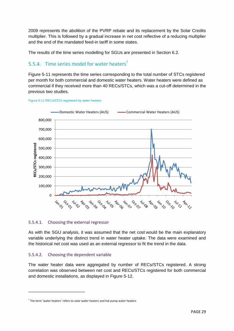
5.5.4. Time series model for water heaters7
Figure 5-11 represents the time series corresponding to the total number of STCs registered
per month for both commercial and domestic water heaters. Water heaters were defined as
commercial if they received more than 40 RECs/STCs, which was a cut-off determined in the
previous two studies.
Figure 5-11 RECs/STCs registered by water heaters
5.5.4.1. Choosing the external regressor
As with the SGU analysis, it was assumed that the net cost would be the main explanatory
variable underlying the distinct trend in water heater uptake. The data were examined and
the historical net cost was used as an external regressor to fit the trend in the data.
5.5.4.2. Choosing the dependent variable
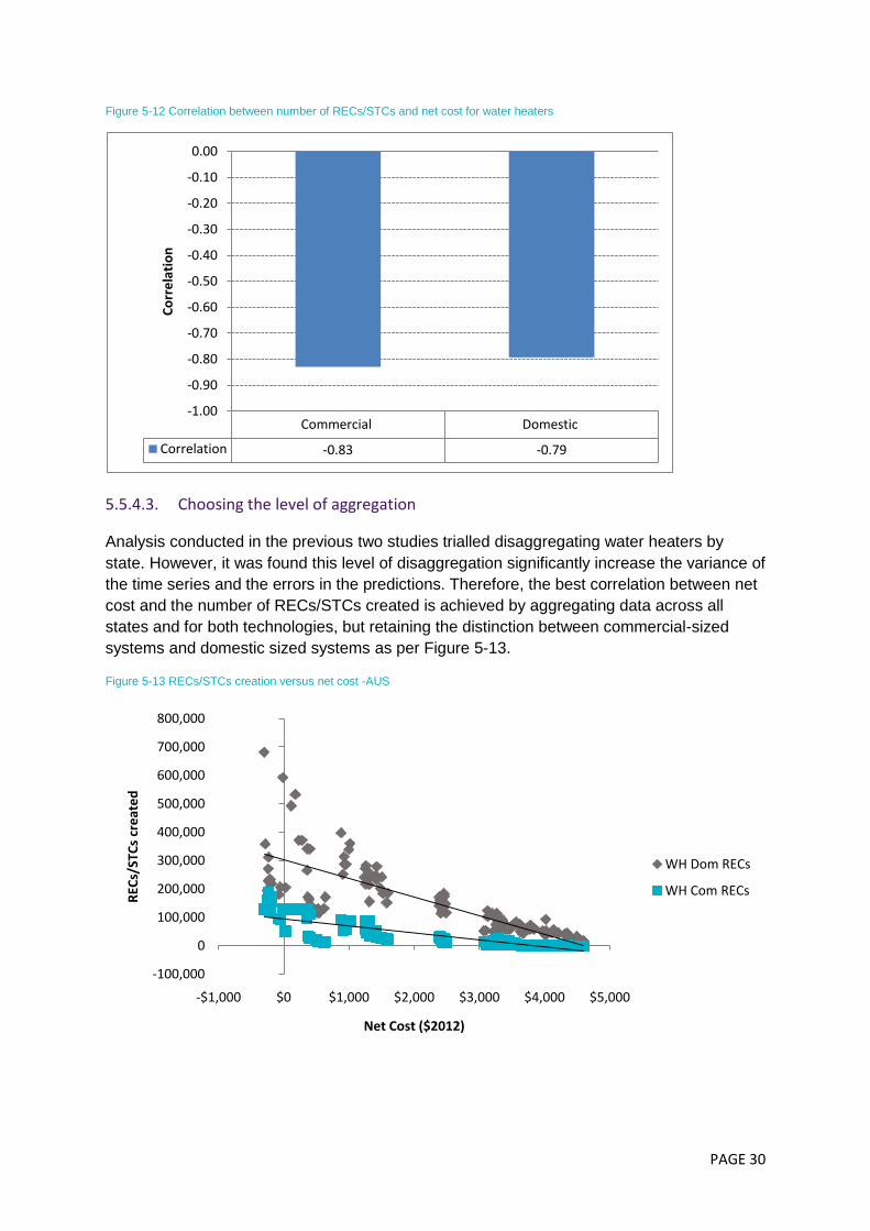
The water heater data were aggregated by number of RECs/STCs registered. A strong
correlation was observed between net cost and RECs/STCs registered for both commercial
and domestic installations, as displayed in Figure 5-12.
7 The term ‘water heaters’ refers to solar water heaters and hat pump water heaters
0
100,000
200,000
300,000
400,000
500,000
600,000
700,000
800,000
REC
s/ST
Cs
regi
ste
red
Domestic Water Heaters (AUS) Commercial Water Heaters (AUS)
PAGE 30
Figure 5-12 Correlation between number of RECs/STCs and net cost for water heaters
5.5.4.3. Choosing the level of aggregation
Analysis conducted in the previous two studies trialled disaggregating water heaters by
state. However, it was found this level of disaggregation significantly increase the variance of
the time series and the errors in the predictions. Therefore, the best correlation between net
cost and the number of RECs/STCs created is achieved by aggregating data across all
states and for both technologies, but retaining the distinction between commercial-sized
systems and domestic sized systems as per Figure 5-13.
Figure 5-13 RECs/STCs creation versus net cost -AUS
Commercial Domestic
Correlation -0.83 -0.79
-1.00
-0.90
-0.80
-0.70
-0.60
-0.50
-0.40
-0.30
-0.20
-0.10
0.00C
orr
ela
tio
n
-100,000
0
100,000
200,000
300,000
400,000
500,000
600,000
700,000
800,000
-$1,000 $0 $1,000 $2,000 $3,000 $4,000 $5,000
REC
s/ST
Cs
cre
ate
d
Net Cost ($2012)
WH Dom RECs
WH Com RECs

PAGE 31
5.5.4.4. Form of the time series model
The original water heater time series were non-stationary, showing both a changing mean
and changing variance over time. However, the logarithm of the original time series was
found to be stationary after the trend was removed. Seasonality in the time series was
insignificant and the data lent itself nicely to an ARIMA model with an external regressor.
In summary, the time series analysis of the data for the water heaters was carried out by
fitting univariate ARIMA models to the logarithm of the monthly number of registered RECs
by water heaters, split into domestic and commercial categories, for all of Australia. The
weighted average of the net cost in each state was used as an external regressor. All of the
modelling was carried out in R.
PAGE 32
6. Modelling results This section presents the results of the modelling for the structural model and the time series
model. The results from the DOGMMA model are presented as the total number of STCs
created from SGU and water heaters for calendar years 2013 to 2015, and the graphs
include historical creation from 2008 until 2012. The results from the time series modelling of
PV are in the form of monthly projected installed capacity, which are then translated into
STC volume projections for the 2013, 2014 and 2015 calendar years. The modelling of water
heaters from the time series are presented as the number of STCs created.
6.1. DOGMMA projections
The results presented in this section are for the total STCs created from PV and water
heaters, however since PV makes up the majority of the units creating STCs, the variations
in trend are nearly entirely attributable to the variation in PV uptake. Additionally, water
heaters are at a more mature stage of market development and the uptake is projected to be
relatively stable.
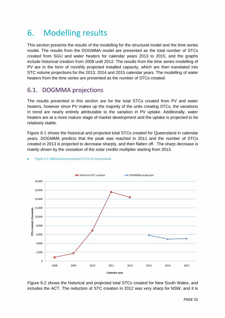
Figure 6-1 shows the historical and projected total STCs created for Queensland in calendar
years. DOGMMA predicts that the peak was reached in 2011 and the number of STCs
created in 2013 is projected to decrease sharply, and then flatten off. The sharp decrease is
mainly driven by the cessation of the solar credits multiplier starting from 2013.
Figure 6-1 Historical and projected STCs for Queensland
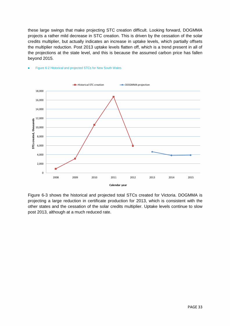
Figure 6-2 shows the historical and projected total STCs created for New South Wales, and
includes the ACT. The reduction of STC creation in 2012 was very sharp for NSW, and it is
0
2,000
4,000
6,000
8,000
10,000
12,000
14,000
16,000
18,000
2008 2009 2010 2011 2012 2013 2014 2015
STC
s cr
eate
d, t
ho
usa
nds
Calendar year
Historical STC creation DOGMMA projection
PAGE 33
these large swings that make projecting STC creation difficult. Looking forward, DOGMMA
projects a rather mild decrease in STC creation. This is driven by the cessation of the solar
credits multiplier, but actually indicates an increase in uptake levels, which partially offsets
the multiplier reduction. Post 2013 uptake levels flatten off, which is a trend present in all of
the projections at the state level, and this is because the assumed carbon price has fallen
beyond 2015.
Figure 6-2 Historical and projected STCs for New South Wales
Figure 6-3 shows the historical and projected total STCs created for Victoria. DOGMMA is
projecting a large reduction in certificate production for 2013, which is consistent with the
other states and the cessation of the solar credits multiplier. Uptake levels continue to slow
post 2013, although at a much reduced rate.
0
2,000
4,000
6,000
8,000
10,000
12,000
14,000
16,000
18,000
2008 2009 2010 2011 2012 2013 2014 2015
STC
s cr
eat
ed
, th
ou
san
ds
Calendar year
Historical STC creation DOGMMA projection

PAGE 34
Figure 6-3 Historical and projected STCs for Victoria
Figure 6-4 shows the historical and projected total STCs created for Tasmania. As with the
other states, the model is projecting a large decrease in 2013, but this is followed by a
flattening off of uptake.
Figure 6-4 Historical and projected STCs for Tasmania
0
1,000
2,000
3,000
4,000
5,000
6,000
7,000
8,000
9,000
2008 2009 2010 2011 2012 2013 2014 2015
STC
s cr
eat
ed
, th
ou
san
ds
Calendar year
Historical STC creation DOGMMA projection
0
100
200
300
400
500
600
2008 2009 2010 2011 2012 2013 2014 2015
STC
s cr
eat
ed
, th
ou
san
ds
Calendar year
Historical STC creation DOGMMA projection
PAGE 35
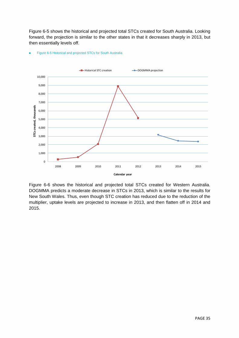
Figure 6-5 shows the historical and projected total STCs created for South Australia. Looking
forward, the projection is similar to the other states in that it decreases sharply in 2013, but
then essentially levels off.
Figure 6-5 Historical and projected STCs for South Australia
Figure 6-6 shows the historical and projected total STCs created for Western Australia.
DOGMMA predicts a moderate decrease in STCs in 2013, which is similar to the results for
New South Wales. Thus, even though STC creation has reduced due to the reduction of the
multiplier, uptake levels are projected to increase in 2013, and then flatten off in 2014 and
2015.
0
1,000
2,000
3,000
4,000
5,000
6,000
7,000
8,000
9,000
10,000
2008 2009 2010 2011 2012 2013 2014 2015
STC
s cr
eat
ed
, th
ou
san
ds
Calendar year
Historical STC creation DOGMMA projection

PAGE 36
Figure 6-6 Historical and projected STCs for Western Australia
Figure 6-7 shows the historical and projected total STCs created for the Northern Territory.
There is a significant drop in STC creation for 2013, reflecting the reduction of the solar
credits multiplier.
Figure 6-7 Historical and projected STCs for Northern Territory
0
1,000
2,000
3,000
4,000
5,000
6,000
7,000
8,000
9,000
2008 2009 2010 2011 2012 2013 2014 2015
STC
s cr
eat
ed
, th
ou
san
ds
Calendar year
Historical STC creation DOGMMA projection
0
20
40
60
80
100
120
140
160
2008 2009 2010 2011 2012 2013 2014 2015
STC
s cr
eat
ed
, th
ou
san
ds
Calendar year
Historical STC creation DOGMMA projection

PAGE 37
Figure 6-8 shows the historical and projected STCs created in aggregate across Australia.
Looking forward, DOGMMA predicts a reduction in the number of STCs created, which is
mainly driven by the cessation of the solar credits multiplier. Certificate production is
projected to stabilise in 2014 and 2015, which could be an indication of the PV industry in
particular reaching maturity.
Figure 6-8 Historical and projected STCs for Australia
6.2. Time series projections
6.2.1. Installed PV Capacity
The results of the time series modelling for all states are presented below. The solid black
line on the left of the graphs represents the historical monthly time series, extending to
December 2012 upon which the projection is based. The radical change to the incentives for
installing PV which occurred in June 20098 threw out the time series model, and sensible
projections could only be achieved by including data from July 2009 onwards, when the
Solar Credits scheme took effect. The green dotted line on the left gravitating around the
solid black line is the model‟s fit to the historical data. The model‟s predicted monthly PV
uptake capacity is represented by the solid red line on the right hand side of the graphs, and
the two dotted lines encompassing the projection represent the prediction plus and minus
the standard error.
8 That is, the abolition of the $8,000 PVRP rebate and the introduction of the Solar Credits scheme.
0
10,000
20,000
30,000
40,000
50,000
60,000
70,000
2008 2009 2010 2011 2012 2013 2014 2015
STC
s cr
eat
ed
, th
ou
san
ds
Calendar year
Historical STC creation DOGMMA projection

PAGE 38
Figure 6-9 shows the historical PV uptake up to December 2012 as well as the time series
projections out to 2015 for Queensland9. The model fits the historical data relatively well as
the movements in the black line and the dotted green line are generally consistent. Based on
the historical data, the monthly installed capacity for new PV systems had peaked in
Queensland in 2012 and will be trending downwards over the next three years. The
government‟s removal of solar credits multiplier is a major contributing factor to the
downward shift in installed capacity as this removes some of the incentive for more uptake.
An expected softer carbon price outlook also lowers incentive for uptake as the avoided cost
of electricity is reduced. Given that PV uptake had already shown a downward trend leading
up to the start of the forecasting period (January 2013), the time series model is reflecting
this trend over the next three years.
Figure 6-9 PV installed capacity projections for Queensland
Figure 6-10 shows the time series projection for the installed monthly PV capacity in New
South Wales. The reduction in projected uptake is not as drastic as projected for
Queensland because the reduction in the NSW FiT occurred long before the corresponding
reduction in the Queensland FiT. Uptake in 2013 is projected to decline gradually, but this is
followed by a flattening off of monthly uptake from mid 2014 until the end of 2015.
9 The error margins in these graphs define 68% confidence intervals.

PAGE 39
Figure 6-10 PV installed capacity projections for New South Wales
Figure 6-11 shows the time series projection for the installed monthly PV capacity in Victoria.
The projection is similar to that of Queensland, where there is an immediate reduction in
uptake capacity, which levels off in early to mid 2013. Uptake is then projected to level off at
a fairly steady rate from mid 2013 until the end of 2015.

PAGE 40
Figure 6-11 PV installed capacity projections for Victoria
Figure 6-12 shows the time series projection for the installed monthly PV capacity in
Tasmania. The projection of capacity uptake is similar to Victoria in that it falls rather sharply,
but then flattens off from mid 2013. The difference however is that uptake is projected to
enter a shallow downtrend, rather than levelling off. This probably reflects the lower levels of
generation achievable by PV in Tasmania.

PAGE 41
Figure 6-12 PV installed capacity projections for Tasmania
Figure 6-13 shows the time series projection for the installed monthly PV capacity in South
Australia. The model fit to the historical time series is reasonably good. The projection has
decreased sharply with the reduction of the solar credits multiplier at the end of December
2012. The trend has similar characteristics to Tasmania, where installed capacity enters a
shallow downtrend after the sharp initial drop.
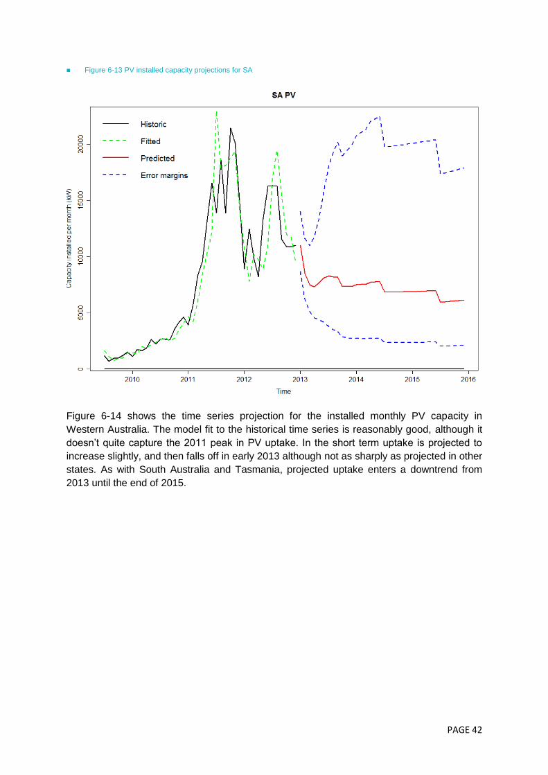
PAGE 42
Figure 6-13 PV installed capacity projections for SA
Figure 6-14 shows the time series projection for the installed monthly PV capacity in
Western Australia. The model fit to the historical time series is reasonably good, although it
doesn‟t quite capture the 2011 peak in PV uptake. In the short term uptake is projected to
increase slightly, and then falls off in early 2013 although not as sharply as projected in other
states. As with South Australia and Tasmania, projected uptake enters a downtrend from
2013 until the end of 2015.

PAGE 43
Figure 6-14 PV installed capacity projections for Western Australia
Figure 6-15 shows the time series projection for the installed monthly PV capacity in the
Northern Territory, with the model fit appearing reasonable. The historical uptake has not
happened as rapidly as in the mainland states, but there appears to have been a sustained,
although somewhat volatile uptrend in uptake. The projection maintains this uptrend until mid
2014, and this is followed by a large step down in installed capacity in mid 2014 and mid
2015.
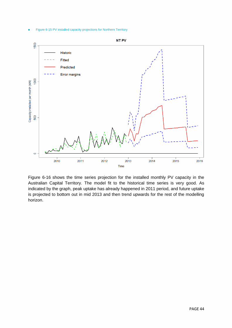
PAGE 44
Figure 6-15 PV installed capacity projections for Northern Territory
Figure 6-16 shows the time series projection for the installed monthly PV capacity in the
Australian Capital Territory. The model fit to the historical time series is very good. As
indicated by the graph, peak uptake has already happened in 2011 period, and future uptake
is projected to bottom out in mid 2013 and then trend upwards for the rest of the modelling
horizon.
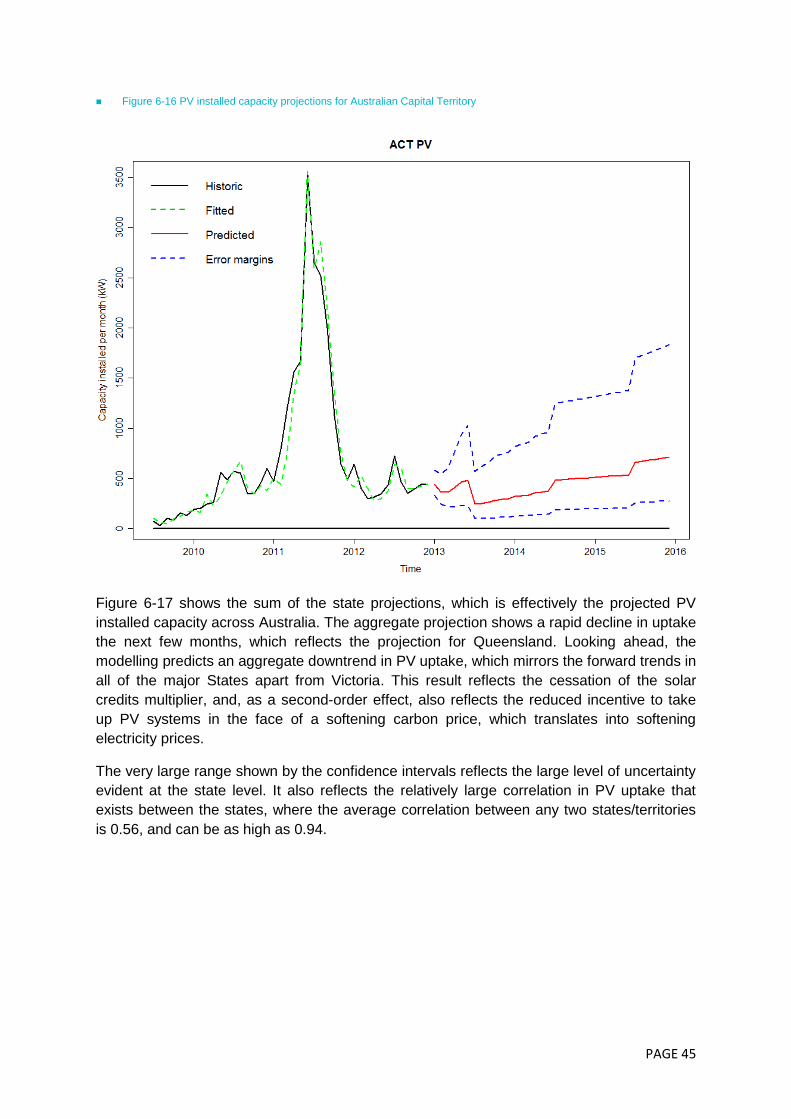
PAGE 45
Figure 6-16 PV installed capacity projections for Australian Capital Territory
Figure 6-17 shows the sum of the state projections, which is effectively the projected PV
installed capacity across Australia. The aggregate projection shows a rapid decline in uptake
the next few months, which reflects the projection for Queensland. Looking ahead, the
modelling predicts an aggregate downtrend in PV uptake, which mirrors the forward trends in
all of the major States apart from Victoria. This result reflects the cessation of the solar
credits multiplier, and, as a second-order effect, also reflects the reduced incentive to take
up PV systems in the face of a softening carbon price, which translates into softening
electricity prices.
The very large range shown by the confidence intervals reflects the large level of uncertainty
evident at the state level. It also reflects the relatively large correlation in PV uptake that
exists between the states, where the average correlation between any two states/territories
is 0.56, and can be as high as 0.94.

PAGE 46
Figure 6-17 PV installed capacity projections aggregated for all Australia
6.2.2. Water heater STC projections
The results of the time series modelling for domestic and commercial water heater STCs
projections are presented below. Unlike the time series modelling for PV systems, most of
the historical time series was able to be employed in projecting water heater STC volumes.
This is because the changes to the government-based financial incentives driving the uptake
of water heaters were not as pronounced as those for SGUs.
Figure 6-18 shows the time series projection for STC volumes created by commercial water
heaters for the whole of Australia. The time series model‟s fit to the historical time series
appears to be reasonably good, although the uncertainty surrounding the projection
indicates that the fit is uncertain, which is likely attributable to the relatively smaller uptake of
commercial systems compared with domestic.
The projection of monthly STC creation from commercial water heaters indicates an initial
reduction in uptake across Australia from current levels which have been trending down
since mid 2012. This seems to be reflecting the latest downtrend in renewable water heater
uptake. The model predicts a recovery to occur at the end of 2013, and then uptake levels
flatten off thereafter.

PAGE 47
Figure 6-18 Commercial water heater STC volume projections for Australia
Figure 6-19 shows the time series projection for STC volumes created by domestic water
heaters for the whole of Australia. The peak in the historical time series around mid 2009
coincides with the pronounced peak exhibited in the corresponding time series for
commercial water heaters and is therefore considered to be somewhat artificially inflated.
However, testing has shown that the effect of this peak does not lead to a large distortion in
projected volumes, and so it was left in the time series unadjusted.
The model‟s fit to the historical time series is quite good and the STC volume projections for
domestic water heaters are similar to those for the commercial category in that there is a
gradual reduction in uptake from current levels, and then a recovery and subsequent
levelling off of uptake from late 2013. The drivers behind this behaviour would be identical to
those described for the commercial category.

PAGE 48
Figure 6-19 Domestic water heater STC volume projections for Australia
6.3. Certificate projections for time series model
Table 6-1 shows the projected number of STCs created by small-scale PV technology by
state for the next three calendar years using the time series model. The reduction of STCs
produced in 2014 relative to 2013 is partly due to the cessation of more government
incentives in that time period, but also reflects the general downtrend in uptake that has
occurred since mid 2012. The STC reduction is spread amongst the States, whereas both
Territories actually increase their STC creation slightly. All of the States have a drop in
certificate creation in 2014 ranging from 20% to 40% relative to 2013. The trend continues
to 2015, although in that case most of the reduction occurs in Queensland.

PAGE 49
Table 6-1 Projected STCs created from PV using time series model10
2013 2014 2015
ACT 108,000 117,000 168,000
Queensland 7,507,000 5,960,000 4,257,000
New South Wales 3,769,000 2,180,000 1,981,000
Victoria 2,560,000 2,020,000 1,947,000
Tasmania 408,000 280,000 266,000
South Australia 2,606,000 2,157,000 1,927,000
Western Australia 2,350,000 1,812,000 1,507,000
Northern Territory 118,000 145,000 80,000
Total 19,425,000 14,670,000 12,133,000
Table 6-2 shows the projected number of STCs created by water heaters by
domestic/commercial classification from the time series model. The water heater forecast
does not vary as much as the PV projection per year as they are more stable.
There is less than a 10% variation in projected certificate creation over the next three years.
Table 6-2 Projected STCs created from water heaters using time series model – Calendar years
2013 2014 2015
Commercial 233,000 290,000 291,000
Domestic 1,499,000 1,595,000 1,596,000
Total 1,732,000 1,885,000 1,886,000
6.3.1. Interpretation of certificate projection for time series model
The time series projections of STC creation tabulated above constitute the central estimate
of the time series model. However, all of the time series projections presented in graphical
form thus far (Figure 6-9 to Figure 6-19) include the 68% confidence intervals around the
central estimate (i.e. one standard error from the projected mean) because the projected
estimate is not just one point, but rather a distribution of possible future outcomes. In other
words, according to the modelling there is a 68% chance that the actual future monthly PV
capacity/STC creation will fall within the 68% confidence intervals.
In order to quantify the range of uncertainty surrounding the total projected annual STC
creation volumes, we calculated the standard deviations of the monthly joint probability
distributions, whose components were all ten projected variables (i.e. the eight state/territory
PV capacities and the two water heater categories). This approach took into account the
correlation that exists between the variables, which was calculated based on the uptake time
series from July 200911 to December 2012. The average correlation in monthly PV uptake
between the states/territories was 0.56, and was as high as 0.94 between Queensland and
Victoria. This high level of positive correlation adds to the uncertainty in the projections.
10 Any discrepancies between the total and the sum of the individual states for this and subsequent tables is due to rounding 11 That is, from the commencement of the Solar Credits multiplier.

PAGE 50
The uncertainty of the projected annual STC volumes is determined by the union of the joint
monthly probability distributions. However, in order to capture the total uncertainty, the
autocorrelation of the uptake time series on a monthly basis also needs to be considered as
it is quite significant. The autocorrelation functions of the monthly Australian PV and water
heater uptake time series are presented in Figure 6-20, which show that even at lags of 10
and 11 months, the autocorrelation is still 0.4 to 0.55. The upshot of this high level of
autocorrelation is that the uncertainty surrounding the projection is further elevated.
Figure 6-20 Autocorrelation of Australian monthly PV and water heater uptake
Combining the twelve monthly distributions for PV and water heaters, we obtained the
following limits, which define the 95% confidence intervals (that is, two standard errors) for
the projected annual STC creation volumes:
Table 6-3 Time series projections with 95% confidence intervals
2013 2014 2015
Lower confidence interval 4,791,000 0 0
Central estimate 21,157,000 16,555,000 14,019,000
Upper confidence interval 37,524,000 35,234,000 29,681,000
For 2014 and 2015, the 95% confidence interval is larger in magnitude than the central
estimate, which is why the lower confidence intervals for these two years are presented as
zero. Table 6-3 reflects the large level of uncertainty evident in Figure 6-9 to Figure 6-17,
which are the PV uptake projections of the individual states and territories. This uncertainty
is ultimately driven by the volatility of monthly PV uptake and is especially present in the
larger states, which have greater influence on the aggregate projection. In addition the large
level of correlation in PV uptake between the states/territories, coupled with the large level of
autocorrelation evident in the Australia-wide monthly PV uptake time series also contributed
0.00
0.10
0.20
0.30
0.40
0.50
0.60
0.70
0.80
0.90
1.00
1 2 3 4 5 6 7 8 9 10 11
Au
toco
rre
lati
on
Monthly lag
Total monthly PV uptake Total monthly Water Heater uptake

PAGE 51
to the large level of uncertainty of the projections. In contrast, the contribution to the
uncertainty from the water heater projections is much smaller.
6.4. Certificate projections for DOGMMA
Table 6-4 shows the projected number of STCs created by PV for each state for the next
three calendar years according to the DOMMA model.
Table 6-4 Projected STCs from PV using DOGMMA – Calendar years
2013 2014 2015
Queensland 5,284,000 4,351,000 4,465,000
New South Wales (inc. ACT) 4,266,000 3,448,000 3,484,000
Victoria 2,965,000 2,404,000 2,443,000
Tasmania 189,000 154,000 157,000
South Australia 3,083,000 2,358,000 2,267,000
Western Australia 3,113,000 2,567,000 2,597,000
Northern Territory 48,000 40,000 41,000
Total 20,855,000 17,355,000 17,498,000
Table 6-5 presents the aggregated projections of STCs created from water heaters for the
next three calendar years according to DOGMMA. The numbers are slightly increasing over
the three years.
Table 6-5 Projected STCs from water heaters using DOGMMA – Calendar years
2013 2014 2015
Total 1,907,000 2,033,000 2,044,000
6.5. Combined STC volume projections
Table 6-6 shows a summary of the STC volume forecast produced by the DOGMMA model
and the forecast produced by the time series model. This is also illustrated in Figure 6-21,
which includes the 95% confidence intervals derived for the time series modelling. Figure
6-21 shows that the projections are quite similar between the two models for the first two
years, and the DOGMMA projection is notably higher in 2015, although it still falls well within
the confidence intervals of the time series projection. This indicates that the time series
model is projecting forward the large downtrend in uptake that commenced in mid 2012 all
the way to 2015.
Table 6-6 Summary of Australia-wide total STC projections
2013 2014 2015
Time series 21,157,000 16,555,000 14,019,000
DOGMMA 20,855,000 17,355,000 17,498,000

PAGE 52
Figure 6-21 Australia-wide STC projections for both models
0
5,000
10,000
15,000
20,000
25,000
30,000
35,000
40,000
2013 2014 2015
STC
s cr
eat
ed
, th
ou
san
ds
Calendar year
DOGMMA
Time series
Time series 95% confidence intervals
PAGE 53
7. Concluding remarks In providing these projections of STC volumes over the 2013, 2014 and 2015 calendar
years, SKM MMA would like to underline the large level of uncertainty surrounding them.
This is evident from the wide range of uncertainty in the time series projections, as indicated
by the large confidence intervals in Figure 6-17 and Figure 6-21.
Whilst the time series model predicts a down trend in STC creation from 2013 to 2015, the
DOGMMA model predicts that STC creation will stabilise by 2015. However, the two models
are in fairly close agreement with each other in their 2013 and 2014 projections with
differences of only 1.4% and 4.6% respectively. The difference in the 2015 projection is
notable, with the time series model predicting the creation of 20% fewer certificates relative
to the DOGMMA model.
The time series model is much more sensitive to short-term trends than the DOGMMA
model since it‟s primarily driven by the immediate trend and the immediate net cost. As a
result, meaningful projections for PV uptake could only be achieved by limiting the time
frame over which the regression to the net cost was performed. This process excluded the
extraordinary levels of uptake witnessed in the market, which generally began in the last
months of 2010. During this time period, the relationship between net cost and uptake broke
down as there was a rush to purchase PV systems in anticipation of the end of various
Government incentive schemes. A similar rush was also observed leading up to July 2012,
and this also contributed to the breakdown of the net cost and uptake relationship. In
addition, the trend towards installation of systems larger than 1.5kW has made the time
series modelling even more uncertain. Therefore the PV installed capacity projections tend
to exhibit large standard errors, with the fundamental source of uncertainty being the lack of
market history at the current level of net installation cost.
SKM MMA has more confidence in the STC volume projections for water heaters produced
by both models. The time series model in particular used almost seven years of market
history to make the predictions. However, these projections only form 8% to 13% of the
annual number of STCs expected to be created over the next three years and therefore do
not carry as much weight as the PV based projections.

PAGE 54
Appendix A DOGMMA model assumptions
A.1 Constraints
A number of constraints that limit the uptake of distributed generation are included in the
model:
Economic constraints. As the capacity of distributed generation in a region increases, the unit cost
of generation also increases12
. This is modelled as reduced capacity factor for all small-scale
technologies as more uptake occurs (in the case of wind, this reflects the fact that as more wind
farms are built, they are likely to locate in less windy areas).
Technical and regulatory constraints. A number of maximum capacity limits are imposed to mimic
the impact of technical limits to uptake in a region or regulatory impediments. The maximum
capacity limits can also be used to model the effect of social issues such as the amenity affect of
wind generation in residential areas and some sensitive sites.
Geographic constraints. The off-take nodes have been divided into metropolitan and rural nodes
and have been utilised to assign the availability of potential capacity in a region for wind and
hydro resources.
General constraint. The capacity of distributed generation is not allowed to exceed the local peak
demand (as this would entail the need to export power to other regions which would incur
additional costs not modelled).
A.2 Local demand
Forecasts of local demand at each node were derived by taking the actual peak demand for
2006/07, as published by state based transmission planners, and then applying the state-
wide peak demand growth rate as forecast by the latest Electricity Statement of
Opportunities. The larger states were represented by multiple nodes, whereas South
Australia and Tasmania were each treated as single node regions.
Energy consumption for each region was calculated from peak demand by using the state-
wide load factor. A correction factor was applied to ensure that the sum of energy
consumption at each node equalled state-wide energy consumption.
A.3 Technical assumptions
Assumed technical parameters for each of the distributed generation options are shown in
Table A.1 . Although the model can handle variations in the assumptions by region, we
assumed that the technical assumptions for each generation technology were the same in
each region. However, the capacity factor for wind generation shown in the table represents
the maximum capacity factor achievable in the region. The actual capacity factor decreases
as the level of wind generation increases within a region.
12 This is done to represent the actual likelihood of rising costs as supply increases, and to avoid what is known as the “flip
flop” effect that occurs with average cost assumptions, where the model chooses nothing but distributed generation once
the cost of distributed generation is lower than the cost of grid supplied electricity.

PAGE 55
Table A- 1 Technical assumptions for distributed generation options
Parameter Rooftop PV Small Wind
Small Hydro
Solar Water Heater
Heat Pump Water Heater
Annual uptake limit as maximum proportion of total demand, %
0.05 – 0.55 0.001 0.0001 0.1 – 0.3 0.1 – 0.3
Maximum plant size
0.001 – 0.01 MW 0.003 – 0.03 MW 0.001 MW 315 litres 315 litres
Capacity factor, % 15 - 18 16 - 38 30 20 - 23 20 - 23
Outage rates, % of year
3 3 3 3 3
Emission intensity of fuel, kt of CO2e/PJ
0.0 0.0 0.0 0.0 0.0
Note: PV capacity factors vary by region according to solar insolation levels. Wind capacity factor varies by the amount of wind
generation in a region. Source: SKM MMA analysis.
It is assumed that in each region, the actual plant size will be equal to maximum allowed size
except for the last plant chosen, which may have a lower capacity.
Unit capital costs are also assumed to decrease over time, reflecting long-term trends. Wind
capital costs are assumed to decline 2% per annum by 2020 and 1% per annum thereafter.
Photovoltaic system capital costs are assumed to decline on average by 2.6% per annum
until 2024 and then at 1.9%, mini hydro systems are assumed to decline at 1% per annum,
whereas SWHs and HPWHs are assumed to be flat in real terms since they are more
mature technologies.
Capital costs are annualised over the life of the plant, assumed to be 15 years for all plants.
Costs are annualised using a real weighted average cost of capital set at 5% above the risk-
free long-term bond rate (which, based on latest 10 year treasury bond rates, is about 2.1%
per annum in real terms).
A.4 Photovoltaic system parameters
A.4.1 Costs
The average installed system cost for residential PV has dropped dramatically over the last
three years and is now around $2,700 per kW in Australia for a typical roof top system.
Figure A- 1 shows the results of some market research conducted by SKMA MMA, where
the quoted installed costs for PV systems excluding subsidies have been plotted against
system size. Smaller systems tend to cost more and larger systems tend to cost less by
achieving some economies of scale and bulk purchase of panels. A fit of an exponential
model relating installed system cost to size yields the following relationship, where x is the
size of the system expressed in kilowatts:
Cost ($/kW) = 2754 exp(-x/117)

PAGE 56
This relationship was used to determine PV costs in the DOGMMA model for the various
system sizes that were modelled.
Figure A- 1 Quoted installed cost for PV systems by system capacity, excluding subsidies
There is an international market for PV modules, which keeps pricing in individual countries
reasonably linked. Module prices increased from 2003 to 2008 due to very strong demand
for PV, driven by strong government incentive programs in countries such as Germany,
Japan and California and a shortage of crystalline silicon feedstock. Manufacturers have
responded by investing heavily in more manufacturing capacity at larger scale to achieve
economies of scale of production. Combining this with a drop in demand due to the financial
crisis and falling subsidy support led to 30% decrease in prices in 2009, with a further fall of
20% in 2010, and another 30% from 2010 prices by 2012.
Predicting the future price of any product is difficult and subject to large uncertainties. The
key parameters that will determine the future cost of PV cells include:
Raw material cost.
Other input costs.
Economic conditions.
Demand and production levels.
Technology.
Many of these parameters are interlinked and improvement in one may force higher costs in
another. For example, as costs fall due to increased economies of scale in manufacturing,
upward cost pressure may result from the increased demand forcing up raw material costs.
$0
$500
$1,000
$1,500
$2,000
$2,500
$3,000
$3,500
$4,000
$4,500
0 1 2 3 4 5 6 7 8 9 10 11
Qu
ote
d in
stal
led
co
st (
$/k
W)
System capacity (kW)

PAGE 57
However, technology improvements may reduce the quantity of raw material required or the
type of material necessary.
Data over the past 25 years have revealed that there has been a 20% cost reduction for
every doubling of the cumulative production of PV cells. This linear behaviour of cost with
cumulative volume is typical of most manufacturing, and is expected to continue at the
historical rate of 20% for each doubling of cumulative production volume. Prices are
projected by the EPIA to fall by 2.6 percent each year in real terms between 2010 and 2020.
SKM MMA‟s assumed installed cost for PV systems over the next ten years is shown in
Figure A- 2.
Figure A- 2 Assumed installed cost for PV systems, 3 kW capacity
A.4.2 Capacity factors
Photovoltaic cell output is directly related to the intensity of the sunlight falling on the panel.
The sunlight intensity or solar insolation varies with global position (effectively distance from
the equator), and local climate, such as cloud cover. Across Australia the solar insolation
varies significantly and the output of a given solar array is dependent on its location. To
account for these variations we have estimated the PV system capacity factors at each of
the transmission nodes employed in the analysis using the RET Screen PV Energy Model13.
The key inputs for this analysis are the geographic coordinates of the locations involved, the
orientation, configuration, and tracking of the panel, and the monthly average temperature
13 RETScreen Energy Project Analysis Software, Clean Energy Decision Support Centre, www.retscreen.net
$0
$500
$1,000
$1,500
$2,000
$2,500
$3,000
2013 2014 2015 2016 2017 2018 2019 2020 2021 2022
Inst
alle
d c
ost
($
/kW
)
PAGE 58
and solar radiation. The climate data are available from the NASA Surface Meteorology and
Solar Energy Data Set14.
The resulting system capacity factors range from 15% (Tasmanian location) to 18%
(northern Australia).
A.5 Solar water heater and heat pump water heater parameters
A.5.1 Costs
Installed costs for solar water heaters and heat pumps were estimated by a survey of
suppliers for the most popular products. It was found that the most popular residential
systems had capacities in the order of 300 litres, with an average installed cost of about
$4900 for solar water heaters and $4800 for heat pump water heaters, excluding rebates.
Since these are mature technologies, it was assumed that projected installed costs would be
flat in real terms.
A.5.2 Energy displaced
SWHs and HPWHs do not actually generate electricity, but rather they displace either
electricity or gas demand (depending on the system they‟ve replaced) by heating water
directly. The amount of energy displaced by these systems was estimated from the typical
number of STCs such systems are entitled to claim, assuming a 15 year life. This ranged
from 1.7 MWh per annum for solar water heaters in Tasmania to 2.0 MWh per annum for
solar water heaters in the northern states. A similar range was also applicable to heat pump
water heaters.
A.6 Small wind parameters
A.6.1 Costs
Distributed wind generation at a scale greater than 0.5 kW has reached a reasonable level of
maturity in the market for off-grid power, and is now becoming available and installed in grid-
connected applications.
Based on available systems in the 0.5 kW to 20 kW size range, and including all ancillary
equipment and installation costs, a correlation between system size and cost has been
developed. These costs are based on retail equipment prices and include GST but do not
include any government rebates or incentives. Costs for grid-connected wind turbines have
become relatively constant over a capacity range of 0.5 kW to 20 kW and are in the vicinity
of $6,500/kW but may increase to around $15,000/kW for sub 0.5 kW units.
A.6.2 Capacity factors
The capacity factor of a wind turbine is a function of the local wind regime and the
generation characteristics of the turbine. As an example we have determined average
annual wind speeds at each of the regional locations utilised in the modelling of the Victorian
nodes using the interactive wind map on the Sustainability Victoria website15. For other
states, we have used data provided by Government authorities or prorated to available wind
generation capacity factors.
14 http://eosweb.larc.nasa.gov/sse/RETScreen/
15 http://www.sustainability.vic.gov.au/www/html/2123-wind-map.asp?intSiteID=4
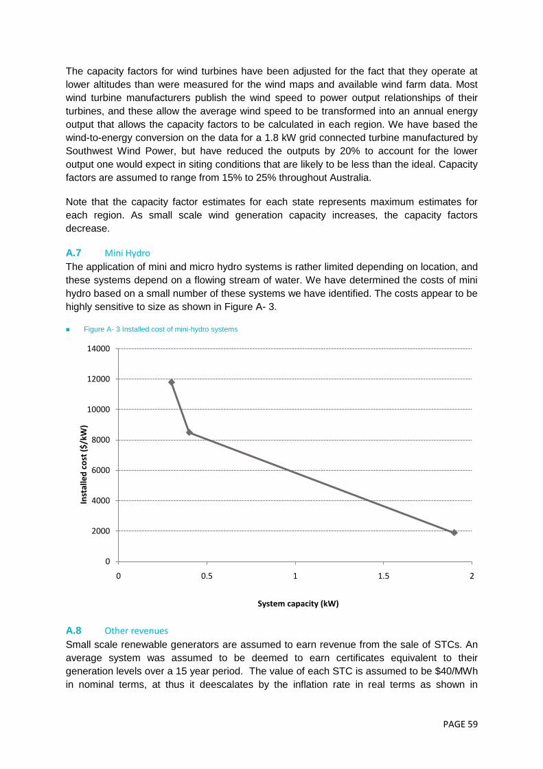
PAGE 59
The capacity factors for wind turbines have been adjusted for the fact that they operate at
lower altitudes than were measured for the wind maps and available wind farm data. Most
wind turbine manufacturers publish the wind speed to power output relationships of their
turbines, and these allow the average wind speed to be transformed into an annual energy
output that allows the capacity factors to be calculated in each region. We have based the
wind-to-energy conversion on the data for a 1.8 kW grid connected turbine manufactured by
Southwest Wind Power, but have reduced the outputs by 20% to account for the lower
output one would expect in siting conditions that are likely to be less than the ideal. Capacity
factors are assumed to range from 15% to 25% throughout Australia.
Note that the capacity factor estimates for each state represents maximum estimates for
each region. As small scale wind generation capacity increases, the capacity factors
decrease.
A.7 Mini Hydro
The application of mini and micro hydro systems is rather limited depending on location, and
these systems depend on a flowing stream of water. We have determined the costs of mini
hydro based on a small number of these systems we have identified. The costs appear to be
highly sensitive to size as shown in Figure A- 3.
Figure A- 3 Installed cost of mini-hydro systems
A.8 Other revenues
Small scale renewable generators are assumed to earn revenue from the sale of STCs. An
average system was assumed to be deemed to earn certificates equivalent to their
generation levels over a 15 year period. The value of each STC is assumed to be $40/MWh
in nominal terms, at thus it deescalates by the inflation rate in real terms as shown in
0
2000
4000
6000
8000
10000
12000
14000
0 0.5 1 1.5 2
Inst
alle
d c
ost
($
/kW
)
System capacity (kW)

PAGE 60
Figure A- 4. It was assumed that the current oversupply in the STC market, which is
depressing the STC price, is only a short term deviation that will correct itself when lower
STPs are published in subsequent years to compensate for the oversupply. The actual STC
price assumed for the modelling commenced from the current market price of about
$30/certificate, tracked back to $40/certificate in nominal dollars over the next two years, and
remained at $40/certificate in nominal dollars thereafter.
Figure A- 4 STC price projections
$28
$29
$30
$31
$32
$33
$34
$35
$36
$37
$38
2013 2014 2015 2016 2017 2018 2019 2020 2021 2022
STC
pri
ce (
$/c
ert
ific
ate
, $2
01
2)