Small noise spectral gap asymptotics for alarge system of nonlinear diffusions

Giacomo Di Gesu∗, Dorian Le Peutrec†

May 19, 2016

Abstract

We study the L2 spectral gap of a large system of strongly coupleddiffusions on unbounded state space and subject to a double-well po-tential. This system can be seen as a spatially discrete approximationof the stochastic Allen-Cahn equation on the one-dimensional torus.We prove upper and lower bounds for the leading term of the spec-tral gap in the small temperature regime with uniform control in thesystem size. The upper bound is given by an Eyring-Kramers-typeformula. The lower bound is proven to hold also for the logarithmicSobolev constant. We establish a sufficient condition for the asymp-totic optimality of the upper bound and show that this condition isfulfilled under suitable assumptions on the growth of the system size.Our results can be reformulated in terms of a semiclassical WittenLaplacian in large dimension.

MSC 2010: 60J60, 76M45, 81Q10, 35P15, 82C22, 60H15.Keywords: Spectral gap, Log-Sobolev inequality, Witten Laplacian, Metasta-bility, Small noise asymptotics, Interacting particle system, Stochastic Allen-Cahn equation.

1 Introduction

This paper concerns the rate of convergence to equilibrium at low tempera-ture of a stochastic interacting particle system, which may be described as

∗CERMICS – Ecole des Ponts ParisTech, 6-8 avenue Blaise Pascal, F-77455 Marne-la-Vallee Cedex 2. (giacomo.di-gesu@enpc.fr)†Departement de Mathematiques, UMR-CNRS 8628, Bat. 425, Universite Paris Sud,

F-91405 Orsay Cedex. (dorian.lepeutrec@math.u-psud.fr)

1

follows. There are N particles, at each time t ≥ 0 the state of the k-th parti-cle is a real random number ξk(t) and the trajectory ξk = (ξk(t))t≥0 satisfiesfor some fixed µ > 1 the stochastic differential equation

dξk =[µξk+1 + ξk−1 − 2ξk

4 sin2 πN

+ ξk − ξ3k

]dt +

√2hN dBk . (1.1)

Here B1 = (B1(t))t≥0, . . . , BN = (BN(t))t≥0 are N independent standardBrownian motions, h is a positive constant and ξN+1 := ξ1, i.e. periodicboundary conditions are assumed. When h > 0 is kept fixed and N islarge, system (1.1) can be seen as a discrete space approximation of thestochastically perturbed Allen-Cahn equation on the interval (0, 2π√

µ):

du(x, t) =[∂2xu(x, t) + u(x, t) − u3(x, t)

]dt +

√2h dW (x, t) , (1.2)

where now (x, t) ∈ (0, 2π√µ)×(0,∞), the boundary condition u(0, t) = u( 2π√

µ, t)

has to be satisfied for every t ≥ 0, and dW is a space-time white noise.Thus, for large N , one might think of ξk(t) ∼ u

(kN

2π√µ, t), and of the chain

ξ(t) = (ξ1(t), . . . , ξN(t)) as giving the position at time t of an elastic ring oflength 2π√

µmoving in a highly viscous, noisy environment and subject to a

simple bistable external force.

Equation (1.2) is a basic and widely studied stochastic partial differentialequation, see e.g. [FaJo, Fun, BDP, GoMa, KORV, Hai2, BeGe, OWW, DaZa,Bar] and references therein. For a more general background on the particlesystem (1.1) we refer to [BFG1, BFG2]. See also [BBM] for aspects closelyrelated to this work. The convergence of (1.1) to (1.2) forN →∞ is discussedin [Bar].

Relaxation properties: heuristics and previous results.

For each fixed h > 0 and number of particles N , the long time behaviourof (1.1) is described by its unique equilibrium distribution, explicitly givenby the probability measure on RN

mh,N(dx) :=e−

V (x)hN dx∫

RN e−V (x)

hN dx,

where the energy function V : RN → R is defined as

V (x) = VN(x) :=N∑k=1

( 1

4x4k −

1

2x2k

)+ µ

N∑k=1

(xk − xk+1)2

8 sin2( πN

)+N

4, (1.3)

2

with xN+1 := x1. This follows from the observation that the drift termin (1.1) is the gradient of V and from general facts about gradient-type diffu-sions. Similarly, for fixed h > 0, there exists a unique equilibrium distributionmh,∞ for the infinite-dimensional system (1.2), see [DaZa,ReVe]. One mightsay that at equilibrium no “phase transition” occurs in the thermodynamiclimit N → ∞. On the contrary, since for each N the energy V admits twolocal minima, given by

I± = I±(N) := ±(1, . . . , 1︸ ︷︷ ︸N entries

) ,

the deterministic dynamics dξ = −∇V (ξ)dt, obtained from (1.1) by settingh = 0, admits two stable equilibrium points. Thus, when h is positive butsmall, the typical picture of a so-called metastable dynamics emerges [FrWe,FaJo, BBM]: the system quickly reaches a local equilibrium in the basin ofattraction of I+ or I−, depending on its initial condition; this local equilibriumendures for a long time, since, in order to be able to explore the whole statespace and distribute according to the global equilibrium mh,N , the system hasto wait for a sufficiently large stochastic fluctuation allowing to overcome theenergetic barrier separating I+ and I−. The critical time scale at whichsuch transitions between minima typically occur is exponentially large in theparameter h. Thus, for h → 0, one observes a significant slowdown in therelaxation towards mh,N .

The aim of this paper is to quantify the mentioned slowdown in the approachto equilibrium of (1.1) when at the same time h is small and N is large.More specifically we shall study for h → 0 and N → ∞ the behaviour ofthe Poincare constant λ(h,N) and the logarithmic Sobolev constant ρ(h,N)of (1.1). These are defined as the largest constants satisfying respectively,for every ϕ ∈ H1(RN ,mh,N), the weighted Poincare inequality

λ(h,N) Varmh,N (ϕ) ≤ hN

∫|∇ϕ|2 dmh,N , (1.4)

and the Gross inequality (or logarithmic Sobolev inequality)

ρ(h,N) Entmh,N (ϕ2) ≤ 2hN

∫|∇ϕ|2 dmh,N . (1.5)

Here Varmh,N and Entmh,N denote the variance and entropy with respect

to mh,N , i.e. Varmh,N (ϕ) :=∫ϕ2dmh,N −

( ∫ϕ dmh,N

)2and, for ϕ ≥ 0,

Entmh,N (ϕ) :=∫ϕ logϕ dmh,N −

∫ϕ dmh,N log

( ∫ϕ dmh,N

). The right

3

hand side of (1.4) is also called the Dirichlet form associated with the Markovprocess defined by (1.1).

It is well-known that the Poincare constant and logarithmic Sobolev constantgive the exponential rate of convergence to equilibrium, respectively in vari-ance and in entropy. We refer e.g. to Theorem 4.2.5 and 5.2.1 in [BGL], whichalso gives a general overview of the interplay between functional inequalitiesand Markov processes. We stress that, from the point of view of spin systemsin statistical mechanics, we are dealing here with the problem of relaxationto equilibrium in a case of continuous unbounded single-spin state space andnonconvex energy function (see e.g. [Led,Zeg,BoHe1,BoHe2] in this context).Concerning exponential convergence of stochastic equations in infinite dimen-sions with fixed noise parameter h we point e.g. to [GoMa,Hai1,Hai2,DaZa].

If N is kept fixed it is known that the leading asymptotic behaviour of λ(h,N)in the limit h→ 0 is given by an Eyring-Kramers-type formula (see [BEGK,BGK, HKN], treating generic multiwell-diffusions in the small noise regime,and also the recent [MeSc, Mic]). More specifically, it follows for examplefrom [HKN] and some straightforward adaptations of their arguments, that

λ(h,N) =1

π

∣∣∣∣det HessV (I−)

det HessV (0)

∣∣∣∣ 12 e−14h

(1 + ε(h,N)

), (1.6)

where the error ε(h,N) satisfies, for h > 0 sufficiently small, |ε(h,N)| ≤CN h. Here CN is some positive constant which may a priori explode in N .On the other hand, as was already observed in [Ste], the prefactor in (1.6) isconvergent in the limit N →∞:

p(N) :=1

π

∣∣∣∣det HessV (I−)

det HessV (0)

∣∣∣∣ 12 −→N→+∞

sinh(π√

2µ−1)

π sin(π√µ−1)

. (1.7)

Similarly, regarding the log-Sobolev constant ρ(h,N), it follows again fromgeneral results (see [MeSc]), that for fixed N the leading term of ρ(h,N) is

again given by p(N)e−14h . We stress that also here, as for the error in (1.6),

there is no control in N on the error term. Thus no rigorous conclusion inthe limit N →∞ can be directly inferred from these results.

On the other hand, rather strong results have been obtained in the analysis ofthe mean time needed for system (1.1) to go from I+ to I−: indeed it has beenshown that an Eyring-Kramers-type formula holds for this transition time,with an error which is uniform in N (see in particular [BBM] and [Bar,BeGe],which extend the results to the infinite-dimensional system (1.2) and even to

4

more general situations). Nevertheless, while the asymptotic relation betweenstochastically defined mean transition times and analytic objects as λ(h,N)is well-established in very general situations for fixed N (see again [BGK]), tothe best of our knowledge there are no rigorous results on how it might behavein the regime of large N , even in the specific model we are considering. In thispaper we do not rely on the mentioned results on mean transition times andrather use purely analytical arguments, partly inspired by the semiclassicalspectral-theoretic approach developped in [HKN].

Statement of the main results

Our first main result below shows that the Eyring-Kramers formula (1.6)provides an upper bound on λ(h,N) with an error term which can indeed beuniformly controlled in the system sizeN . Moreover it provides a quantitativelower bound at logarithmic scale on ρ(h,N) which is independent of N . Inparticular it ensures that ρ(h,N) and λ(h,N) do not degenerate for anyfixed h. One might say that no “dynamical phase transition” occurs in thethermodynamic limit N →∞ (see also [GoMa]).

Theorem 1.1. For every δ > 0 there exists a constant Cδ > 0 such that forevery h > 0 and every N ∈ N

Cδ e− 3+2

√2+δ

24h e−14h ≤ ρ(h,N) ≤ λ(h,N) ≤ p(N) e−

14h

(1 + ε(h,N)

),

where the prefactor p(N) is given by (1.7) and the error term ε(h,N) satisfies

∃C > 0 s.t. ∀h ∈ (0, 1] , ∀N ∈ N , |ε(h,N)| ≤ C h .

The exponential decay in h given by the lower bound in Theorem 1.1 ap-pears to be rather rough, but unfortunately, when insisting to get boundswith uniform control in N , it is for the moment not clear how one couldobtain a substantial improvement, even when focusing only on λ(h,N). Forthe latter one can exploit the spectral theory of self-adjoint operators: thegenerator of the Markovian semigroup giving the evolution of (1.1) is indeedthe differential operator

Lh = Lh,N := −hN∆ + ∇V · ∇ . (1.8)

The closure in L2(mh,N) of Lh acting on C∞c (RN), which we still denote byLh, is self-adjoint and nonnegative, admits 0 as eigenvalue and has purelydiscrete spectrum for each h,N fixed (see Section 2.2 for more details). Asa consequence of the Max-Min principle, its spectral gap, defined as its firstnonzero eigenvalue, coincides with λ(h,N).

5

According to our second main result below, the problem of obtaining theEyring-Kramers formula as lower bound for λ(h,N) can then be reduced tothe problem of proving a suitable separation between λ(h,N) and the nexteigenvalue of Lh. More precisley, the existence of a uniform lower boundon the “second spectral gap” in a certain regime in which N possibly growsto infinity, turns out to be sufficient for the validity of the Eyring-Kramersformula in the same regime:

Theorem 1.2. Assume there exist constants h0, δ > 0 and, for each h ∈(0, h0], a set N (h) ⊂ N such that

∀h ∈ (0, h0] , ∀N ∈ N (h) , Spec(Lh) ∩ ]λ(h,N), λ(h,N)+δ[ = ∅ . (1.9)

Thenλ(h,N) = p(N) e−

14h

(1 + ε(h,N)

),

where the prefactor p(N) is given by (1.7) and the error term ε(h,N) satisfies

∃C > 0 s.t. ∀h ∈ (0, h0] , ∀N ∈ N (h) , |ε(h,N)| ≤ C h .

Our last main theorem implies that there exist regimes with unbounded Nunder which the Eyring-Kramers formula (1.6) holds with bounded errorε(h,N). Indeed, in order to be in the situation of Theorem 1.2, it is enough

that N grows slower than h−34 :

Theorem 1.3. Let C > 0 and α ∈ (0, 34). Then there exist constants h0, δ >

0 such that condition (1.9) in Theorem 1.2 is fulfilled with

N (h) =N ∈ N : N ≤ Ch−α

.

The above results concerning λ(h,N) can be equivalently reformulated interms of splitting properties of the ground state of a specific semiclassicalSchrodinger operator in large dimension. This is a consequence of the well-known ground state transformation, see e.g. [JMS]: up to conjugation with

e−V

2hN and some N -dependent dilatation (see Subsection 2.2 for more details),the operator hLh turns out to be unitarily equivalent to the operator actingin the flat space L2(dx) and defined through

∆(0)f,h := −h2∆ + |∇f |2 − h∆f , where f(x) :=

V (√Nx)

2N. (1.10)

We like to mention that a semiclassical Schrodinger operator having the formof ∆

(0)f,h, with f a generic smooth function, is also called semiclassical Witten

6

Laplacian associated to f . The superscript (0) stresses that we consider onlyoperators on functions, the Witten Laplacian being more generally definedthrough a supersymmetric extension on the full algebra of differential forms.The operator acting on p-forms is commonly denoted by ∆

(p)f,h and connects

in the semiclassical limit h → 0 topological properties of the underlyingmanifold to the topology of the energy landscape induced by f [Wit, HeSj,CFKS].

We stress that, even if one focuses only on the operator ∆(0)f,h acting on func-

tions (that is, equivalently on the diffusion operator Lh, as in the presentpaper), the enlarged supersymmetric point of view may provide further in-sights and a powerful technical tool. We refer especially to [Sjo3, Joh, Hel2,Hel3,HKN,KuTa,HeNi1,HeNi2,Lep,Dig,BHM,LeNi] for works in this spiritand the links between statistical mechanics and Witten Laplacians. In partic-ular, as was recognized in [HKN], the operator ∆

(1)f,h acting on 1-forms, being

related for h→ 0 to the energetic bottlenecks responsible for the slowdown ofthe underlying stochastic process, appears rather naturally when analyzingthe low-lying eigenvalues of ∆

(0)f,h.

We emphasize that semiclassical techniques as WKB expansions, Agmon es-timates and harmonic approximation for Schrodinger operators, used e.g.in [HKN], are generally not uniformly controlled in the limit N → ∞ (seehowever [BaMø, MaMø] for previous works dealing with Witten Laplaciansin large dimension and also [Sjo1, Sjo2, Hel1, Hel3] and references therein).Also for the specific model we consider here, the arguments of [HKN] do notcarry over with uniform bounds in N .

Comments on the techniques used in this paper

Though inspired by the supersymmetric approach of [HKN], in this paper we

do not make explicit use of ∆(1)f,h. Indeed, a careful analysis of the energy V

permits to construct a very efficient global quasimode passing through thebottleneck and connecting the two minima of V (see Definition 3.10). Thisconstruction, together with a precise analysis of Laplace integrals in largedimension, enables us to give the upper bound of Theorem 1.1.

For the lower bound in Theorem 1.1, we depart from the semiclassical ap-proach and rather exploit perturbation techniques for fixed h. These permit,even though for general µ > 1 the function V is not convex outside a com-pact set, to reduce to the case of a convex energy and then to apply thewell-known Bakry-Emery criterion. We use here that the interaction partin the energy V is strong enough to ensure good relaxation properties forlarge N . Thus, roughly speaking, we regard the energy coming from the

7

single particle double-well potential as a perturbation of the interaction part.This is opposed to the perturbative regime considered in previous worksas [BoHe1,BoHe2]: in these references the interaction constant µ is tuned ina way that it is rather the interaction part to become a perturbation of thesingle particle potential.

The relevant quantity naturally appearing in the estimates leading to Theo-rem 1.2 is the quotient of quadratic forms defined, for any ϕ in the domainof Lh, by

E(ϕ) :=

∫RN |Lhϕ|

2 dmh,N

hN∫RN |∇ϕ|2 dmh,N

.

To connect to the existing literature, we point out that, after integration byparts, this quantity can be equivalently rewritten in the two forms

E(ϕ) =

∫RN Γ2(ϕ) dmh,N∫RN Γ(ϕ) dmh,N

=

∫RN(L

(1)h ∇ϕ

)· ∇ϕ dmh,N

hN∫RN |∇ϕ|2 dmh,N

. (1.11)

Here Γ, Γ2 are respectively the carre du champ operator and its iteration(see for example [BGL] for more details about this notion) and L

(1)h :=

Lh ⊗ Id + hN HessV is an operator acting on vector fields (i.e. 1-forms),

related to ∆(1)f,h via ground state transformation. The last expression in (1.11)

can be generalized by allowing, instead of ∇ϕ, more general, non-gradientvector fields. This is one of the main advantages of the supersymmetric ap-proach and is crucially exploited in works as [HKN,HeNi1,Lep,LeNi], or [Dig]in a discrete setting. In the arguments we give here we do not use this addi-tional freedom since we can work with the gradient of the quasimode alreadyexploited in the proof of Theorem 1.1 and thus streamline both the resultsand the presentation.

For the proof of Theorem 1.3 we shall adopt the Schrodinger point of viewand thus work with ∆

(0)f,h. We combine here standard localization techniques

for the analysis of semiclassical Schrodinger operators [CFKS] and a two-scaleanalysis naturally adapted to the structure of the energy V .

Plan of the paper

The rest of the paper is organized as follows. In Section 2 we discuss basicproperties of the model and the precise relation between the diffusion opera-tor Lh and the Schrodinger operator ∆

(0)f,h. Sections 3, 4 and 5 are respectively

devoted to the proofs of Theorems 1.1, 1.2 and 1.3.

Subsection 3.2, which might also be of independent interest, provides a sharp

8

Laplace-type asymptotics for the normalization constant Zh,N :=∫RN e

−V (x)hN dx

when h→ 0 with uniform control in N .

2 Basic properties of the model

The aim of this section is to fix our notation and to provide some basicbackground information on our model which we shall use throughout in therest of the analysis. We denote by 〈·, ·〉 the standard scalar product in RN ,by ‖ ·‖, or | · | when no ambiguity is possible, the corresponding Hilbert normand, more generally, for p ∈ N we write

‖x‖p :=( N∑k=1

|xk|p) 1p .

The gradient, Hessian and (negative) Laplacian acting on functions in RN

are denoted respectively by ∇,Hess and ∆.

2.1 Properties of V and related Gaussian estimates

Throughout the paper we fix a µ > 1. The energy function V , definedin (1.3), can be rewritten in a more compact notation as

V (x) =1

4‖x‖4

4 +1

2〈x, (K − 1)x〉 +

N

4, (2.1)

where K : RN → RN is a normalised discrete Laplacian, defined by settingfor x ∈ RN and k ∈ 1, . . . , N,

(Kx)k :=µ

4 sin2( πN

)

(2xk − xk+1 − xk−1

). (2.2)

It is understood that xN+1 := x1 and x0 := xN , which corresponds to periodicboundary conditions. It holds 〈x,Kx〉 = 〈Kx, x〉 and, according to our choiceof sign, 〈x,Kx〉 ≥ 0. The operator K is diagonalised through the discreteFourier transform x ∈ RN of x ∈ RN , defined by

xk :=1√N

N∑j=1

xj e−i2π j

Nk .

More precisely we have for every k ∈ 0, . . . , N − 1,

(Kx)k = νk xk , where νk := µsin2(k π

N)

sin2( πN

). (2.3)

9

Note that ν0 = 0 is a simple eigenvalue of K and that its smallest non-zero eigenvalue equals µ for every N ∈ N, N ≥ 2. We shall denote byP : RN → RN the projection onto the eigenspace of K corresponding tothe eigenvalue 0 and by P⊥ := 1 − P the projection onto its orthogonalcomplement. Note that RanP = Span(1, . . . , 1) so that P associates tox ∈ RN the constant vector with components the mean of x: for everyk ∈ 1, . . . , N,

(Px)k = x :=1

N

N∑j=1

xj =x0√N

. (2.4)

For shortness the range RanP of P will sometimes also be denoted by C,and we refer to it as the space of constant states, or the “diagonal” of RN .Similarly we write C⊥ := RanP⊥ for the space of states orthogonal to theconstants.

We mention here explicitly the following simple identities, which we shallfrequently use in the sequel:

∀x ∈ RN ,N∑k=1

(P⊥x)k = 0 and ‖Px‖ =√Nx = x0 .

The fact that the first non-zero eigenvalue of K equals µ implies the followingdiscrete Poincare-type inequality:

∀ρ ∈ [0, µ] , ∀x ∈ RN , 〈x,Kx〉 ≥ ρ(‖x‖2 − 〈x, Px〉

). (2.5)

For more information on the discrete Fourier transform and discrete Lapla-cian, see for example [Ter].

Some basic features of the energy landscape determined by V are the fol-lowing. First, it is straightforward to check that the constant states givenby

I+ := (1, . . . , 1) , I− := (−1, . . . ,−1) and O := (0, . . . , 0) ,

are critical points of V , i.e. satisfy ∇V (x) = 0, for every N ∈ N. Moreover

HessV (I±) = K + 2 and HessV (O) = K − 1 . (2.6)

It follows from (2.3) that K + 2 admits only strictly positive eigenvalues,while K − 1 has one simple eigenvalue −1 and, since µ > 1, all the others

10

are strictly positive. The identities (2.6) imply therefore in particular thatI± are local minima and O is a saddle point, i.e. a critical point of index 1.The additive constant N

4appearing in (2.1) is chosen such that

V (I±) = 0 and V (O) =N

4. (2.7)

A crucial feature of the model, implied by the assumption µ > 1, is thefollowing. When restricted to the N−1 dimensional subspace C⊥ = RanP⊥,the quadratic form HessV is strictly convex, uniformly in N and x ∈ RN .Indeed, according to the discrete Poincare inequality given in (2.5), for everyx and w ∈ RN ,

〈w,HessV (x)w〉 ≥ 〈w, (K − 1)w〉 ≥ (µ− 1) ‖w‖2 − µ〈w,Pw〉 .

In particular one gets the lower bound

∀x ∈ RN , ∀w ∈ C⊥ , 〈w,HessV (x)w〉 ≥ (µ− 1) ‖w‖2 . (2.8)

The latter inequality can be used to show that I+, I− and O are the onlycritical points of V (see also [BFG1]):

Lemma 2.1. Fix N ∈ N and let x ∈ RN \ O, I+, I−. Then ∇V (x) 6= 0.

Proof. Estimate (2.8) implies that for each c ∈ R there can be at most onecritical point of the restriction V |Hc of V to the hyperplane Hc := x ∈ RN :x = c. Since for every c ∈ R the constant vector c := (c, . . . , c) ∈ C satisfies

∀w ∈ C⊥ , 〈∇V (c), w〉 = (c3 − c)N∑k=1

wk = 0 , i.e ∇ (V |Hc)(c) = 0 ,

the critical points of V necessarily have to be on the diagonal C. The state-ment of the lemma follows now by noting that for c := (c, . . . , c)

V (c) = N( 1

4c4 − 1

2c2 +

1

4

).

Since, according to (2.6), the quadratic part of V around its critical points isessentially given by the discrete Laplacian K, part of our analysis will rely ona good control in large dimension of Gaussian integrals, whose covariances

11

are given by the resolvent of K or slight perturbations thereof. To be specific,we shall consider for suitable α, β ∈ R operators Q : RN → RN of the form

Q :=(αP + K + β

)−1, (2.9)

where P is the projection given by (2.4). Note that the particular caseα = 0, β = 2 corresponds to Q = (K + 2)−1, which according to (2.6) equalsthe inverse of the Hessian of V at the minima. Taking instead α = 2, β = −1,one obtains Q = (2P +K − 1)−1, which is the inverse of the Hessian of V atthe saddle point, modulo inverting sign of its unique negative eigenvalue.In general, for any choice of α, β such that Q is well-defined, it followsfrom (2.3) that for each k ∈ 0, . . . , N − 1 it holds (Qx)k = σk xk, wherethe eigenvalues are now given by

σk =1

νk + βfor k ∈ 1, . . . , N − 1 and σ0 =

1

α + β.

In particular, Q is positive in the sense of quadratic forms if and only ifα+ β > 0 and µ+ β > 0, which is assumed from now on. A crucial propertyof Q is that it is of trace class, uniformly in the dimension:

∃C > 0 : ∀N ∈ N , Tr Q :=N−1∑k=0

σk < C . (2.10)

The latter estimate is obtained by straightforward estimates on the νk’s (es-sentially νk ∼ µk2, see their expression in (2.3)). We remark en passantthat (2.10) fails to hold in the case of higher-dimensional single particle state,i.e. xk ∈ Rd with d > 1. This is linked to well-known difficulties in the an-alytical treatment of the Stochastic Allen-Cahn equation in higher spatialdimension. A straightforward consequence of (2.10) is a uniform control inN of moments of the centered Gaussian distribution with covariance Q whosedensity is given by

dµ =e−〈x,Q−1x〉

2((2π)N detQ

) 12

dx .

In particular we will repeatedly exploit in this paper the following uniformbound, which we state here for later reference.

Lemma 2.2. Let Q be defined as in (2.9) with α + β > 0 and µ + β > 0.Then there exists a constant C > 0 such that for p ∈ 4, 6 and every h > 0,N ∈ N,

1((2πhN)N detQ

) 12

∫RNN−1‖x‖pp e−

〈x,(hNQ)−1x〉2 dx ≤ Ch

p2 . (2.11)

12

Proof. Differentiating suitably the moment generating function of a Gaussianwith covariance Q, given by

∀ ξ ∈ RN ,1(

(2π)N detQ) 1

2

∫RNe−〈x,Q−1x〉

2 e〈x,ξ〉 dx = e〈ξ,Qξ〉

2 ,

yields for the left hand side of (2.11) the expression

CpN

N∑k=1

(hNQk,k)p2 , with C4 = 3, C6 = 15 . (2.12)

Using the “Fourier integral representation” of Q we get for its diagonal termsthe expression Qk,k = 1

N

∑N−1j=0 σj for every k. It follows that (2.12) equals

hp2Cp(

∑N−1k=0 σk)

p2 . This yields the desired result thanks to (2.10).

For convenience of the reader, we also state explicitly the following simpletail estimate, which will be exploited throughout the paper. Recall that xdenotes the mean of x ∈ RN as defined in (2.4).

Lemma 2.3. Let Q be defined as in (2.9) with α + β > 0 and µ + β > 0.

Then for every r > 0, the following estimate holds for C = C(r) = (α+β)r2

2

and for every h ∈ (0, 1] and N ∈ N,

1((2πhN)N detQ

) 12

∫|x|>r

e−〈x,(hNQ)−1x〉

2 dx ≤(h

πC

) 12

e−Ch .

Proof. Diagonalising Q via the Fourier transform and recalling that x = x0√N

,we obtain

1((2πhN)N detQ

) 12

∫|x|>r

e−〈x,(hNQ)−1x〉

2 dx =2√2π

∫y0>r√

α+βhe−

y202 dy0

and the statement boils down to the standard Gaussian tail-estimate:

∀η > 0 ,

∫ +∞

η

e−t2

2 dt ≤ 1

ηe−

η2

2 . (2.13)

13

Lastly, the ratio of the determinants of HessV (I+) and HessV (0) converges,as already observed in [Ste] (see also [BBM, BeGe]). More precisely thefollowing statement holds true:

Lemma 2.4. The relation (1.7) mentioned in the introduction holds true:√det HessV (I+)

| det HessV (0)|=

√det HessV (I−)

| det HessV (0)|−→

N→+∞

sinh(π√

2µ−1)

sin(π√µ−1)

. (2.14)

Proof. According to (2.6) and to (2.3), we have for 2 ≤ N ∈ N,

det HessV (I±)

| det HessV (0)|=

det(K + 2)

| det(K − 1)|=

N−1∏k=0

νk + 2

|νk − 1|= 2

N−1∏k=1

νk + 2

νk − 1,

so we want to show that

√2

√√√√N−1∏k=1

νk + 2

νk − 1=√

2N−1∏k=1

(1 +

3

νk − 1

) 12

−→N→+∞

cµ ,

where cµ is given by

cµ :=sinh(π

√2µ−1)

sin(π√µ−1)

=√

2+∞∏k=1

µk2 + 2

µk2 − 1,

the last equality being a direct consequence of Euler’s product formula

∀ z ∈ C , sin(πz) = πz+∞∏k=1

(1− z2

k2

).

Noticing now the relation

N−1∏k=1

(1 +

3

νk − 1

) 12

=

(1 +

3

µ 1sin2( π

N)− 1

)12N(N)

2 bN−12c∏

k=1

(1 +

3

νk − 1

),

we are then lead to prove that

bN−12c∏

k=1

(1 +

3

νk − 1

)−→

N→+∞

+∞∏k=1

µk2 + 2

µk2 − 1= lim

N→+∞

bN−12c∏

k=1

(1 +

3

µk2 − 1

),

and it is therefore sufficient to show that

bN−12c∏

k=1

1 + 3νk−1

1 + 3µk2−1

=

bN−12c∏

k=1

(1 + 3

νk − µk2

(νk − 1)(µk2 + 2)

)−→

N→+∞1 . (2.15)

14

The end of the proof follows from the computations done in [BBM] pp. 331-332 but we give the details for the sake of completeness. From the inequalities

∀x ∈ [0,π

2] , 0 ≤ x2(1− x2

3) = x2 − x4

3≤ sin2 x ≤ x2 ,

we deduce that for every 2 ≤ N ∈ N and k ∈ 1, . . . , bN−12c,

µ k2(1− π2

12) ≤ µ k2

(1− π2k2

3N2

)≤ νk ≤

3µN2k2

3N2 − π2, (2.16)

and therefore

−µπ2k4

3N2≤ νk − µ k2 ≤ µπ2k2

3N2 − π2,

from which we obtain that for every N ≥ 2 and k ∈ 1, . . . , bN−12c,

|νk − µ k2| ≤ 2µπ2k4

N2. (2.17)

It follows from (2.16) and (2.17) that there exist 2 ≤ N0 ∈ N and a positiveconstant C such that for every N ≥ N0 and k ∈ bN0−1

2c, . . . , bN−1

2c,∣∣∣∣3 νk − µ k2

(νk − 1)(µk2 + 2)

∣∣∣∣ ≤ C

N2.

Using the inequality | ln(1 + x)| ≤ |x|1−|x| valid on (−1, 1), we get that for

every N 3 N ≥ maxN0,√C + 1,

∣∣∣ ln bN−12c∏

k=bN0−12c

(1 + 3

νk − µk2

(νk − 1)(µk2 + 2)

)∣∣∣ ≤ bN−12c∑

k=bN0−12c

C

N2 − C−→

N→+∞0 ,

and the equation (2.15) we were looking for follows, since for any fixed k,

1 + 3 νk−µk2(νk−1)(µk2+2)

goes to 1 when N → +∞.

For additional background on Gaussian measures and perturbations thereofin large and infinite dimensions we point to [GlJa,Sim,Dap].

2.2 Relation between Lh and the Witten Laplacian

As already mentioned in the introduction, all the results stated there canequivalently be reformulated in terms of Witten Laplacians using the ground

15

state transformation. More precisely, up to a multiplicative factor hN−1, theoperator Lh := −hN∆+∇V ·∇ acting on L2(e−

VhN dx) is unitarily equivalent

to a semiclassical Witten Laplacian acting on the flat L2(dx):

e−fh hLh e

fh = N

(− h2∆ + |∇f |2 − h∆f

)=: N ∆

(0)

f ,h, (2.18)

where

f(x) :=V (x)

2N.

Using in addition the unitary dilatations Dilλ on L2(dx), which are defined,

for any λ > 0 and any g ∈ L2(dx), by Dilλg := λN2 g(λ ·), we have also the

unitary equivalence

Dil√N N∆(0)

f ,hDil 1√

N= −h2∆ + |∇f |2 − h∆f =: ∆

(0)f,h , (2.19)

where

f(x) := f(√Nx) =

V (√Nx)

2N.

Note that ∆(0)f,h =

∑j(∂j + h∂jf)∗ (∂j + h∂jf) with domain C∞c (RN) is sym-

metric and nonnegative in L2(dx), that its Schrodinger potential |∇f |2−h∆fis smooth and, for fixed h and N , tending to infinity as |x| → ∞ . It followsthen from standard arguments of the theory of Schrodinger operators (see

e.g. [Hel4, Proposition 7.10 and Theorem 9.15]) that ∆(0)f,h is essentially self-

adjoint on C∞c (RN), and that its closure, which we still denote by ∆(0)f,h, has

compact resolvent and therefore purely discrete spectrum. Notice moreover

that ker ∆(0)f,h = Span(e−

fh ) .

Due to (2.18) and (2.19), these properties can be immediately transferred

from ∆(0)f,h to Lh and it holds

Spec(∆(0)f,h) = h Spec(Lh) . (2.20)

3 Uniform bounds in the dimension

This section is devoted to the establishment of lower bounds on the log-Sobolev constant ρ(h,N) (defined through (1.5)) and upper bounds on thespectral gap λ(h,N) (defined through (1.4)), which are uniform in the systemsize N . The main results here are the following.

16

Theorem 3.1 (Lower Bound). For every δ > 0, there exists a positive con-stant Cδ such that the log-Sobolev constant ρ(h,N) satisfies

∀h > 0 ,∀N ∈ N , Cδ e− 3+2

√2+δ

24h e−14h ≤ ρ(h,N) .

Theorem 3.2 (Upper Bound). The spectral gap λ(h,N) satisfies for everyh > 0 and N ∈ N the inequality

λ(h,N) ≤ p(N) e−14h

(1 + ε(h,N)

),

where the prefactor p(N) is given by (1.7) and the error term ε(h,N) satisfies

∃C > 0 s.t. ∀h ∈ (0, 1] , ∀N ∈ N , |ε(h,N)| ≤ C h .

Note that, together with the well-known inequality ρ(h,N) ≤ λ(h,N), whichis easily obtained by applying (1.5) to 1 + εu and letting ε→ 0, Theorem 3.1and Theorem 3.2 yield Theorem 1.1.

The proof of Theorem 3.1 is based on a careful perturbation of the energyV and a combination of the Holley-Stroock perturbation principle and theBakry-Emery criterion for log-Sobolev constants (c.f. Proposition 3.3 andProposition 3.4 below). The proof of Theorem 3.2 relies on a suitable choiceof a test function (or “quasimode”) and exploits a good control on the nor-

malisation constant Zh,N :=∫RN e

−V (x)hN dx.

This section is organised as follows. Subsection 3.1 contains the proof ofTheorem 3.1. Subsection 3.2, which might also be of independent interest,provides a sharp Laplace-type asymptotics for Zh,N when h→ 0 with uniformcontrol in N . Finally, Subsection 3.3 contains the proof of Theorem 3.2.

3.1 Proof of Theorem 3.1 (Lower Bound on ρ(h,N))

Our proof is based on a combination of the following two well-known criteriafor establishing lower bounds on the log-Sobolev constant (see for exam-ple [Roy, Prop. 3.1.18 and Theorem 3.1.29] or the original papers [HoSt],[BaEm]).

We fix here N ∈ N and use the following standard notation: for a measurablefunction U : RN → R such that e−U ∈ L1(RN , dx), we define the probabilitymeasure dmU := Z−1

U e−Udx, where ZU :=∫RN e

−U dx is the normalisationconstant. Moreover we write for nonnegative u ∈ C∞c (RN ;R),

EntmU (u) :=

∫RNu log u dmU −

∫RNu log

(∫RNu dmU

)dmU ,

17

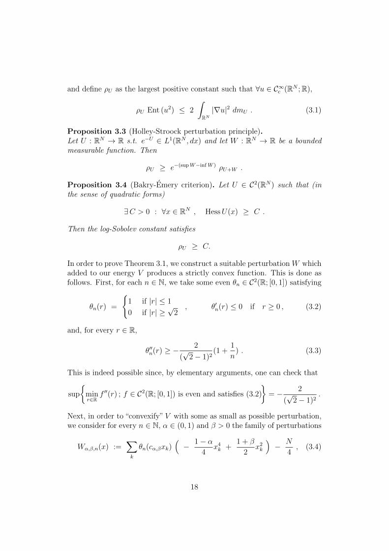
and define ρU as the largest positive constant such that ∀u ∈ C∞c (RN ;R),

ρU Ent (u2) ≤ 2

∫RN|∇u|2 dmU . (3.1)

Proposition 3.3 (Holley-Stroock perturbation principle).Let U : RN → R s.t. e−U ∈ L1(RN , dx) and let W : RN → R be a boundedmeasurable function. Then

ρU ≥ e−(supW−inf W ) ρU+W .

Proposition 3.4 (Bakry-Emery criterion). Let U ∈ C2(RN) such that (inthe sense of quadratic forms)

∃C > 0 : ∀x ∈ RN , HessU(x) ≥ C .

Then the log-Sobolev constant satisfies

ρU ≥ C.

In order to prove Theorem 3.1, we construct a suitable perturbation W whichadded to our energy V produces a strictly convex function. This is done asfollows. First, for each n ∈ N, we take some even θn ∈ C2(R; [0, 1]) satisfying

θn(r) =

1 if |r| ≤ 1

0 if |r| ≥√

2, θ′n(r) ≤ 0 if r ≥ 0 , (3.2)

and, for every r ∈ R,

θ′′n(r) ≥ − 2

(√

2− 1)2(1 +

1

n) . (3.3)

This is indeed possible since, by elementary arguments, one can check that

sup

minr∈R

f ′′(r) ; f ∈ C2(R; [0, 1]) is even and satisfies (3.2)

= − 2

(√

2− 1)2.

Next, in order to “convexify” V with some as small as possible perturbation,we consider for every n ∈ N, α ∈ (0, 1) and β > 0 the family of perturbations

Wα,β,n(x) :=∑k

θn(cα,βxk)(− 1− α

4x4k +

1 + β

2x2k

)− N

4, (3.4)

18

where cα,β :=√

1−α1+β

. Since the polynomial part of (3.4) is nonnegative on

supp θn(cα,β ·), one gets from 0 ≤ θn ≤ 1 the two bounds

− N

4≤ Wα,β,n(x) ≤ N

4

( (1 + β)2

1− α− 1

), (3.5)

valid for every n ∈ N, α ∈ (0, 1), β > 0 and every x ∈ RN . Moreover, for asuitable choice of the parameters α, β and n, the Wα,β,n–perturbation of theoriginal energy V becomes a uniformly strictly convex function:

Lemma 3.5. Let α ∈ ( 13(2−

√2)2+1

, 1). Then there exists n0 ∈ N such that for

any β > 0 and n ≥ n0, we have in the sense of quadratic forms:

∃Cα,β,n > 0 s.t. ∀x ∈ RN , ∀N ∈ N , Hess(V +Wα,β,n

)(x) ≥ Cα,β,n .

Proof. Recalling the definition (1.3) of V and that the discrete Laplacian µKis nonnegative we get the estimate

∀x ∈ RN , ∀α, β > 0, ∀n ∈ N , Hess(V +Wα,β,n

)(x) ≥ HessUα,β,n(x) ,

where

Uα,β,n :=1

4

∑k

(1−(1−α)θn(cα,βxk)

)x4k −

1

2

∑k

(1−(1+β)θn(cα,βxk)

)x2k .

The Hessian of Uα,β,n is diagonal and we have, for any k ∈ 1, . . . , N:

∂2kUα,β,n (x) = c2

α,βθ′′n(cα,βxk)

(− 1− α

4x4k +

1 + β

2x2k

)︸ ︷︷ ︸

I

+

+ 2cα,βθ′n(cα,βxk)

(− (1− α)x3

k + (1 + β)xk

)︸ ︷︷ ︸

II

+

+ θn(cα,βxk)(− 3(1− α)x2

k + (1 + β))

+ 3x2k − 1︸ ︷︷ ︸

III

.

Case 1: |cα,βxk| >√

2.Then θn = θ′n = θ′′n = 0 for every n ∈ N and we obtain

∀α, β > 0 , ∂2kUα,β,n(x) = 3x2

k − 1 ≥ 6(1 + β)

1− α− 1 ≥ 5 .

19

Case 2: |cα,β,nxk| < 1.Then θ′n = θ′′n = 0, θn = 1 for every n ∈ N and we obtain

∀α, β > 0 , ∂2kUα,β,n(x) = 3αx2

k + β ≥ β .

Case 3: cα,βxk ∈ [1,√

2].First, for every β > 0, α ∈ (0, 1), n ∈ N, we have, using θ′n(cα,βxk) ≤ 0 (seeindeed (3.2)) and

(− (1− α)x3

k + (1 + β)xk)≤ 0, that II ≥ 0.

Moreover, we deduce from(3(1 − α)x2

k − (1 + β))≥ 0 that the term III

satisfies

III = (1− θn(cα,βxk))(

3(1−α)x2k − (1 +β)

)+ 3αx2

k +β ≥ 3αx2k +β .

Let us lastly look at the term I. Since(− 1−α

4x4k + 1+β

2x2k

)≥ 0, we have

0 ≤ c2α,β

(− 1− α

4x4k +

1 + β

2x2k

)= x2

k c2α,β

(− 1− α

4x2k +

1 + β

2

)≤ x2

k

(− 1− α

4+

1− α2

)=

1

4(1− α) x2

k ,

and so, since θ′′n(cα,βxk) ≥ −2(√

2−1)2(1 + 1

n) according to (3.3),

I ≥ −(1 +1

n)

1− α(2−

√2)2

x2k .

Summing up, we then have in Case 3:

∀α, β > 0 , ∂2kUα,β,n(x) ≥

α(3(2−

√2)2 + 1 + 1

n

)− 1− 1

n

(2−√

2)2x2k + β . (3.6)

If α > 13(2−

√2)2+1

as in the assumption, there exists n0 ∈ N such that the right

hand side of (3.6) is bigger than or equal to β and hence strictly positive forany n ≥ n0.

The case cα,βxk ∈ [−√

2,−1] can be treated in an analogous way and thusthe lemma is proven.

The proof of Theorem 3.1 can now be easily concluded: for any δ > 0, wemay pick α ∈ ( 1

3(2−√

2)2+1, 1) close to 1

3(2−√

2)2+1and some sufficiently small

β > 0 such that

1 + δ

4+

3 + 2√

2

24=

3(2−√

2)2(1 + δ) + 1

12(2−√

2)2≥ (1 + β)2

4(1− α). (3.7)

20

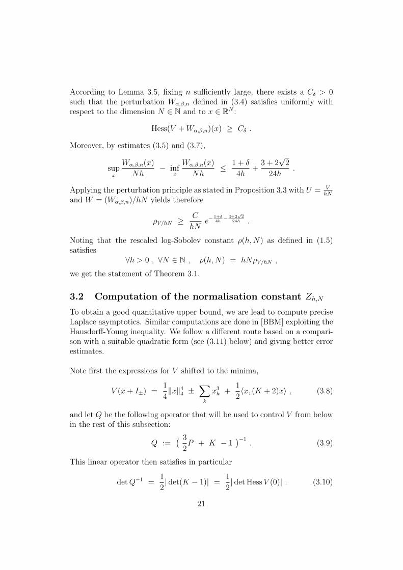
According to Lemma 3.5, fixing n sufficiently large, there exists a Cδ > 0such that the perturbation Wα,β,n defined in (3.4) satisfies uniformly withrespect to the dimension N ∈ N and to x ∈ RN :

Hess(V +Wα,β,n)(x) ≥ Cδ .

Moreover, by estimates (3.5) and (3.7),

supx

Wα,β,n(x)

Nh− inf

x

Wα,β,n(x)

Nh≤ 1 + δ

4h+

3 + 2√

2

24h.

Applying the perturbation principle as stated in Proposition 3.3 with U = VhN

and W = (Wα,β,n)/hN yields therefore

ρV/hN ≥C

hNe−

1+δ4h− 3+2

√2

24h .

Noting that the rescaled log-Sobolev constant ρ(h,N) as defined in (1.5)satisfies

∀h > 0 , ∀N ∈ N , ρ(h,N) = hNρV/hN ,

we get the statement of Theorem 3.1.

3.2 Computation of the normalisation constant Zh,N

To obtain a good quantitative upper bound, we are lead to compute preciseLaplace asymptotics. Similar computations are done in [BBM] exploiting theHausdorff-Young inequality. We follow a different route based on a compari-son with a suitable quadratic form (see (3.11) below) and giving better errorestimates.

Note first the expressions for V shifted to the minima,

V (x+ I±) =1

4‖x‖4

4 ±∑k

x3k +

1

2〈x, (K + 2)x〉 , (3.8)

and let Q be the following operator that will be used to control V from belowin the rest of this subsection:

Q :=( 3

2P + K − 1

)−1. (3.9)

This linear operator then satisfies in particular

detQ−1 =1

2| det(K − 1)| =

1

2| det HessV (0)| . (3.10)

21

Lemma 3.6. Let Q : RN → RN be the linear operator defined through equa-tion (3.9). Then the following two estimates hold:

∀x ≥ −1 , V (x+ I+) ≥ 1

2〈x,Q−1x〉 , (3.11)

and

∀ |x| ≤ 1 ,1

4‖x‖4

4 −∣∣∑

k

x3k

∣∣ +1

2〈x, (K + 2)x〉 ≥ 1

2〈x,Q−1x〉 . (3.12)

Proof. Note first the following estimate implied by Holder’s inequality:

∀x ∈ RN , ‖x‖44 ≥ Nx4 . (3.13)

It follows that

1

4‖x‖4

4 −N

2x2 +

N

4≥ N

4x4 − N

2x2 +

N

4=

N

4(x− 1)2(x+ 1)2 ,

and therefore

V (x) ≥ N

4(x− 1)2(x+ 1)2 +

1

2〈x, (K − 1)x〉 +

N

2x2

=N

4(x− 1)2(x+ 1)2 +

1

2〈x, (P +K − 1)x〉 , (3.14)

where the last inequality follows from the relation Nx2 = 〈x, Px〉.From (3.14), since P + K − 1 annihilates constants, we get for the shiftedpotential the estimate

V (x+ I+) ≥ N

4x2 +

1

2〈x, (P +K − 1) x〉 for x ≥ −1 , (3.15)

which proves (3.11). Note moreover that (3.14) also gives

∀x ≤ 1 , V (x+ I−) ≥ 1

2〈x,Q−1x〉 , (3.16)

which is actually equivalent to (3.11) due to the symmetry of V . Esti-mate (3.12) is then an immediate consequence of the expressions for V (x+I+)and V (x+ I−) given in (3.8) and (3.11), (3.16).

Proposition 3.7. For every r > 0 there exists a constant C > 0 such thatfor each h ∈ (0, 1] and N ∈ N,∫

x≥0 ; |x−1|≥re−

V (x)hN dx ≤ C−1 (2πhN)

N2

| det HessV (I+)| 12e−

Ch . (3.17)

22

Proof. Fix r > 0. Shifting the origin to the minimum I+ and using thequadratic lower bound given in (3.11) of Lemma 3.6, we get

I :=

∫x≥0 ; |x−1|≥r

e−V (x)hN dx ≤

∫x≥−1 ; |x|≥r

e−〈x,(hNQ)−1x〉

2 dx ,

where Q : RN → RN is the positive operator defined in (3.9). According tothe Gaussian tail estimate of Lemma 2.3, there exists a constant C > 0 suchthat for every h ∈ (0, 1] and N ∈ N,

I ≤ C−1 (2πhN)N2(

detQ−1) 1

2

e−Ch .

The desired result follows now from (3.10) and the convergence of the ratioof determinants given by (2.14) of Lemma 2.4.

Proposition 3.8. Let r ∈ (0, 1]. Then∫|x−1|≤r

e−V (x)hN dx =

(2πhN)N2

| det HessV (I+)| 12(

1 + εr(h,N)), (3.18)

where the error term εr(h,N) satisfies

∃C = C(r) > 0 s.t. ∀h ∈ (0, 1] , ∀N ∈ N , |εr(h,N)| ≤ C h .

Proof. Fix r ∈ (0, 1]. Shifting the origin to the minimum I+ (recall (3.8))and isolating the contribution of the integral given by the non-quadratic partof V from the rest, we write∫|x−1|≤r

e−V (x)hN dx =

∫|x|≤r

e−V (x+I+)

hN dx

=

∫|x|≤r

e−〈x,(K+2)x〉

2hN dx︸ ︷︷ ︸=:I

+

∫|x|≤r

a(x) e−〈x,(K+2)x〉

2hN dx︸ ︷︷ ︸=:II

, (3.19)

with

a(x) := exp(−

14‖x‖4

4 +∑

k x3k

hN

)− 1 .

23

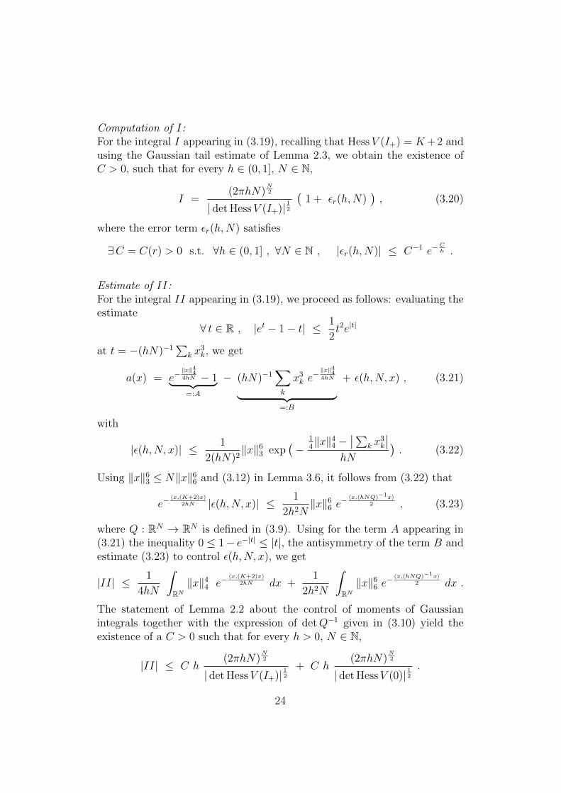
Computation of I:For the integral I appearing in (3.19), recalling that HessV (I+) = K+2 andusing the Gaussian tail estimate of Lemma 2.3, we obtain the existence ofC > 0, such that for every h ∈ (0, 1], N ∈ N,

I =(2πhN)

N2

| det HessV (I+)| 12(

1 + εr(h,N)), (3.20)

where the error term εr(h,N) satisfies

∃C = C(r) > 0 s.t. ∀h ∈ (0, 1] , ∀N ∈ N , |εr(h,N)| ≤ C−1 e−Ch .

Estimate of II:For the integral II appearing in (3.19), we proceed as follows: evaluating theestimate

∀ t ∈ R , |et − 1− t| ≤ 1

2t2e|t|

at t = −(hN)−1∑

k x3k, we get

a(x) = e−‖x‖444hN − 1︸ ︷︷ ︸=:A

− (hN)−1∑k

x3k e− ‖x‖

44

4hN︸ ︷︷ ︸=:B

+ ε(h,N, x) , (3.21)

with

|ε(h,N, x)| ≤ 1

2(hN)2‖x‖6

3 exp(−

14‖x‖4

4 −∣∣∑

k x3k

∣∣hN

). (3.22)

Using ‖x‖63 ≤ N‖x‖6

6 and (3.12) in Lemma 3.6, it follows from (3.22) that

e−〈x,(K+2)x〉

2hN |ε(h,N, x)| ≤ 1

2h2N‖x‖6

6 e− 〈x,(hNQ)−1x〉

2 , (3.23)

where Q : RN → RN is defined in (3.9). Using for the term A appearing in(3.21) the inequality 0 ≤ 1− e−|t| ≤ |t|, the antisymmetry of the term B andestimate (3.23) to control ε(h,N, x), we get

|II| ≤ 1

4hN

∫RN‖x‖4

4 e−〈x,(K+2)x〉

2hN dx +1

2h2N

∫RN‖x‖6

6 e− 〈x,(hNQ)−1x〉

2 dx .

The statement of Lemma 2.2 about the control of moments of Gaussianintegrals together with the expression of detQ−1 given in (3.10) yield theexistence of a C > 0 such that for every h > 0, N ∈ N,

|II| ≤ C h(2πhN)

N2

| det HessV (I+)| 12+ C h

(2πhN)N2

| det HessV (0)| 12.

24

Recalling the convergence of the ratio of determinants given by (2.14) ofLemma 2.14, we finally obtain

∃C > 0 : ∀h > 0 , ∀N ∈ N , |II| ≤ C h(2πhN)

N2

| det HessV (I+)| 12. (3.24)

Putting together (3.20) and (3.24) gives the statement of the proposition.

According to the symmetry of V , Propositions 3.7 and 3.8 finally lead to theprecise computation of the normalisation constant Zh,N :

Corollary 3.9. For the normalisation constant Zh,N we have

Zh,N :=

∫RNe−

V (x)hN dx = 2

(2πhN)N2

| det HessV (I+)| 12(

1 + ε(h,N)), (3.25)

where the error term ε(h,N) satisfies

∃C > 0 s.t. ∀h ∈ (0, 1] , ∀N ∈ N , |ε(h,N)| ≤ C h .

3.3 Upper Bound on λ(h,N)

We give in this subsection the proof of Theorem 3.2. We recall that forx ∈ RN ,

x :=1

N

N∑k=1

xk ,

and we consider in the rest of this subsection the following operator Q, whoseinverse is HessV (O) modulo inverting sign of its unique negative eigenvalue,

Q := (2P +K − 1)−1 . (3.26)

We have then in particular the relation

detQ−1 = | det(K − 1)| = | det HessV (0)| . (3.27)

Definition 3.10. Let χ = χh,N : RN → [−1, 1] be the function defined by

χ(x) :=2√

2πhN

∫ √Nx0

e−t2

2hN dt =2√2πh

∫ x

0

e−t2

2h dt .

For h > 0 let ψ = ψh,N : RN → R be given by

ψ(x) :=χ(x)( ∫

RN χ2(x) e−

V (x)hN dx

) 12

.

25

Remark 3.11. Note that by antisymmetry, the quasimode ψ has mean zero:∫RNψ(x)e−

V (x)hN dx = 0 .

Lemma 3.12. The square of the weighted L2-norm of χ satisfies∫RNχ2(x) e−

V (x)hN dx = 2

(2πhN)N2

| det HessV (I+)| 12(

1 + ε(h,N)),

where the error term ε(h,N) satisfies

∃C > 0 s.t. ∀h ∈ (0, 1] , ∀N ∈ N , |ε(h,N)| ≤ C h . (3.28)

Proof. By the symmetry of V and χ2 and splitting the integral we get∫RNχ2(x) e−

V (x)hN dx = 2

∫x≥0

χ2(x) e−V (x)hN dx

= 2

∫|x−1|≤ 1

2χ2(x) e−

V (x)hN dx︸ ︷︷ ︸

=:I

+ 2

∫x≥0 ; |x−1|≥ 1

2χ2(x) e−

V (x)hN dx︸ ︷︷ ︸

=:II

.

Using for the term I the simple estimate

∃C > 0 : ∀x ∈ |x− 1| ≤ 1

2 , ∀h ∈ (0, 1] , |χ(x)− 1| ≤ C−1 e−

Ch ,

and Proposition 3.8, and for the term II the bound |χ| ≤ 1 and Proposi-tion 3.7, we get∫

RNχ2(x) e−

V (x)hN dx = 2

(2πhN)N2

| det HessV (I+)| 12(

1 + ε(h,N)), (3.29)

where the error term ε(h,N) satisfies (3.28).

Theorem 3.2 is then a direct consequence of the following proposition:

Proposition 3.13. The function ψ from Definition 3.10 satisfies for everyh > 0 and every N ∈ N,

hN

∫RN|∇ψ|2 e−

V (x)hN dx =

1

π

∣∣∣∣det HessV (I−)

det HessV (0)

∣∣∣∣ 12 e−14h

(1 + ε(h,N)

),

where the error term ε(h,N) satisfies

∃C > 0 s.t. ∀h ∈ (0, 1] , ∀N ∈ N , |ε(h,N)| ≤ C h .

26

Proof. Since for every x ∈ RN ,

hN |∇χ|2(x) =2

πe−

x2

h =2

πe−〈x,2Px〉2hN ,

we get with Q as defined in (3.26),

hN

∫RN|∇χ|2 e−

V (x)hN dx =

2

π

∫RNe−〈x,(hNQ)−1x〉

2 dx

+2

π

∫RNe−〈x,(hNQ)−1x〉

2

(e−‖x‖444hN − 1

)dx .

From this equality, the expression of the determinant of Q given in (3.27),and from the inequality 0 ≤ 1− e−|t| ≤ |t|, we obtain the following estimatealso using the uniform bounds on Gaussian moments provided by Lemma 2.2,

hN

∫RN|∇χ|2 e−

V (x)hN dx =

2

π

(2πhN)N2

| det HessV (0)| 12(

1 + ε(h,N)), (3.30)

where the error term ε(h,N) satisfies (3.13). Combining this with Lemma 3.12finishes the proof.

4 Sharp spectral gap asymptotics

In this section, we prove Theorem 1.2. To do so, we will again use the testfunction ψ introduced in Definition 3.10 in order to show that it asymptoti-cally saturates the inequality

∀ϕ ∈ D(Lh) s.t. ‖ϕ‖L2(e−

VhN )

= 1 , λ(h,N) ≤ hN

∫RN|∇ϕ|2e−

V (x)hN dx

under a further assumption on the separation between the second and thethird eigenvalues of Lh. Under this condition, we can indeed reverse thisinequality up to an error term involving the quantity

E(ϕ) :=

∫RN |Lhϕ|

2 e−V (x)hN dx

hN∫RN |∇ϕ|2e

−V (x)hN dx

,

which was already mentioned in the introduction.

Proposition 4.1. Let δ, h0 > 0 and, for every h ∈ (0, h0], N (h) ⊂ N s.t.

∀h ∈ (0, h0] , ∀N ∈ N (h) , Spec(Lh) ∩ [0, δ) = 0, λ(h,N) . (4.1)

27

Then, for all h ∈ (0, h0], N ∈ N (h) and ϕ := ϕh,N ∈ D(Lh) satisfying∫RNϕ2e−

V (x)hN dx = 1 ,

∫RNϕ e−

V (x)hN dx = 0 ,

∫RNϕ(Lhϕ)e−

V (x)hN dx <

δ

2, (4.2)

we have the lower bound

λ(h,N) ≥ hN

∫RN|∇ϕ|2e−

V (x)hN dx

(1 − ε(h,N)

),

where the error term ε(h,N) satisfies

0 ≤ ε(h,N) ≤ min

1 ,2hN

δ

∫RN|∇ϕ|2e−

V (x)hN dx+

2√δ

√E(ϕ)

.

The proof is a simple application of the following standard Markov-typeinequality, which is a consequence of the spectral theory for self-adjoint op-erators.

Lemma 4.2. Let T be a nonnegative self-adjoint operator on a Hilbert spaceH with domain D. Then for every u ∈ D and every b > 0,

‖1[b,∞)(T )u‖2 ≤ 〈Tu, u〉b

.

Proof of Proposition 4.1. We denote respectively by 〈·, ·〉 and ‖ · ‖ the scalar

product and the Hilbert norm in L2(e−VhN ), and by P := 1[0,δ)(Lh) the spec-

tral projector of Lh onto the interval [0, δ). From∫RNϕ(Lhϕ)e−

V (x)hN dx = hN

∫RN|∇ϕ|2e−

V (x)hN dx ,

using the third point of the property (4.2) together with Lemma 4.2, we get

‖(1− P )ϕ‖2 = ‖1[δ,+∞)(Lh)ϕ‖2 ≤ hN

δ‖∇ϕ‖2 <

1

2. (4.3)

In particular, since ‖ϕ‖ = 1, we have also

‖Pϕ‖2 = ‖ϕ‖2 − ‖(1− P )ϕ‖2 ≥ 1

2, (4.4)

and so Pϕ 6= 0. We can therefore define u := Pϕ‖Pϕ‖ . Since moreover 〈ϕ, 1〉 = 0,

we have 〈Pϕ, 1〉 = 〈ϕ, P1〉 = 0 . Thus, using also (4.1), u is necessarilya normalised eigenfunction of Lh associated with the eigenvalue λ(h,N).

28

Consequently, it follows from LhP = PLh on D(Lh), the self-adjointness ofP = P 2, and elementary rearrangements of terms, that

λ(h,N) = 〈u, Lhu〉 =〈Pϕ,LhPϕ〉‖Pϕ‖2

=〈ϕ,Lhϕ〉‖Pϕ‖2

+〈Pϕ− ϕ,Lhϕ〉‖Pϕ‖2

= hN‖∇ϕ‖2[1 +

‖(1− P )ϕ‖2

‖Pϕ‖2︸ ︷︷ ︸=:I

+〈(P − 1)ϕ,Lhϕ〉hN‖∇ϕ‖2︸ ︷︷ ︸

=:II

(1 +

‖(1− P )ϕ‖2

‖Pϕ‖2

)︸ ︷︷ ︸

=:III

].

The statement of the proposition follows now by observing that, accordingto (4.3) and (4.4),

I ≤ 2hN

δ‖∇ϕ‖2 , |II| ≤ ‖Lhϕ‖√

δ hN‖∇ϕ‖, and III ≤ 2 ,

and λ(h,N) is nonnegative.

Applying Proposition 4.1 with the test function ψ as defined in Defini-tion 3.10, the statement of Theorem 1.2 is then a direct consequence of thequasimodal estimates given in Proposition 3.13 and in the following propo-sition:

Proposition 4.3. Let ψ be the test function introduced in Definition 3.10.Then there exists C > 0 such that for every h ∈ (0, 1] and every N ∈ N,∫

RN|Lhψ|2 e−

V (x)hN dx ≤ C h2

∣∣∣∣det HessV (I−)

det HessV (0)

∣∣∣∣ 12 e−14h . (4.5)

Proof. A straightforward computation, whose details are given below for thesake of completeness, leads to the identity∫

RN|Lhχ|2 e−

V (x)hN dx =

2

πhN2

∫RN

( N∑k=1

x3k

)2e−

V (x)+〈x,Px〉hN dx . (4.6)

Hence, using the estimate(∑N

k=1 x3k

)2 ≤ N‖x‖66 implied by the Cauchy-

Schwarz inequality, we obtain the bound

0 ≤∫RN|Lhχ|2 e−

V (x)hN dx ≤ 2 e−

14h

πhN

∫RN‖x‖6

6 e− 〈x,(hNQ)−1x〉

2 dx , (4.7)

where Q is defined in (3.26). The estimate (4.5) follows by applying theuniform moment bound of Lemma 2.2 to the right hand side of (4.7), recalling

29

the expression (3.27) of the determinant ofQ and finally invoking Lemma 3.12

for∫RN χ

2e−V (x)hN dx.

To show (4.6) and thus completing the proof, we note that for k ∈ 1, . . . , N,

∂kχ(x) =1

N

2√2πh

e−x2

2h =1

N

2√2πh

e−〈x,Px〉2hN ,

and compute

Lhχ = −hN eV (x)hN

N∑k=1

∂k(e−

V (x)hN ∂kχ

)= − 2√

2πhNe−〈x,Px〉2hN

N∑k=1

(− ∂kV (x) + x

)=

2√2πhN

e−〈x,Px〉2hN

N∑k=1

x3k ,

where for the last inequality we used∑N

k=1(Kx)k = 0. Taking the square weget (4.6).

5 Lower bound on the second spectral gap

The aim of this section is to prove Theorem 1.3. Instead of working directlywith the diffusion operator Lh, we switch to the Schrodinger operator pointof view and consider the semiclassical Witten Laplacian on functions actingin the flat L2(dx) and given by

∆(0)f,h = −h2∆ + |∇f |2 − h∆f ,

where f : RN → R is defined as

f(x) :=V (√Nx)

2N=

N

8‖x‖4

4 +1

4〈x, (K − 1)x〉 +

1

8. (5.1)

Note that due to the rescaling of variables, the two minima of f are rescaledby a factor

√N with respect to the minima of V . More precisely they are

given by

J+ :=I+√N

=1√N

(1, . . . , 1) , J− :=I−√N

=1√N

(−1, . . . ,−1) .

30

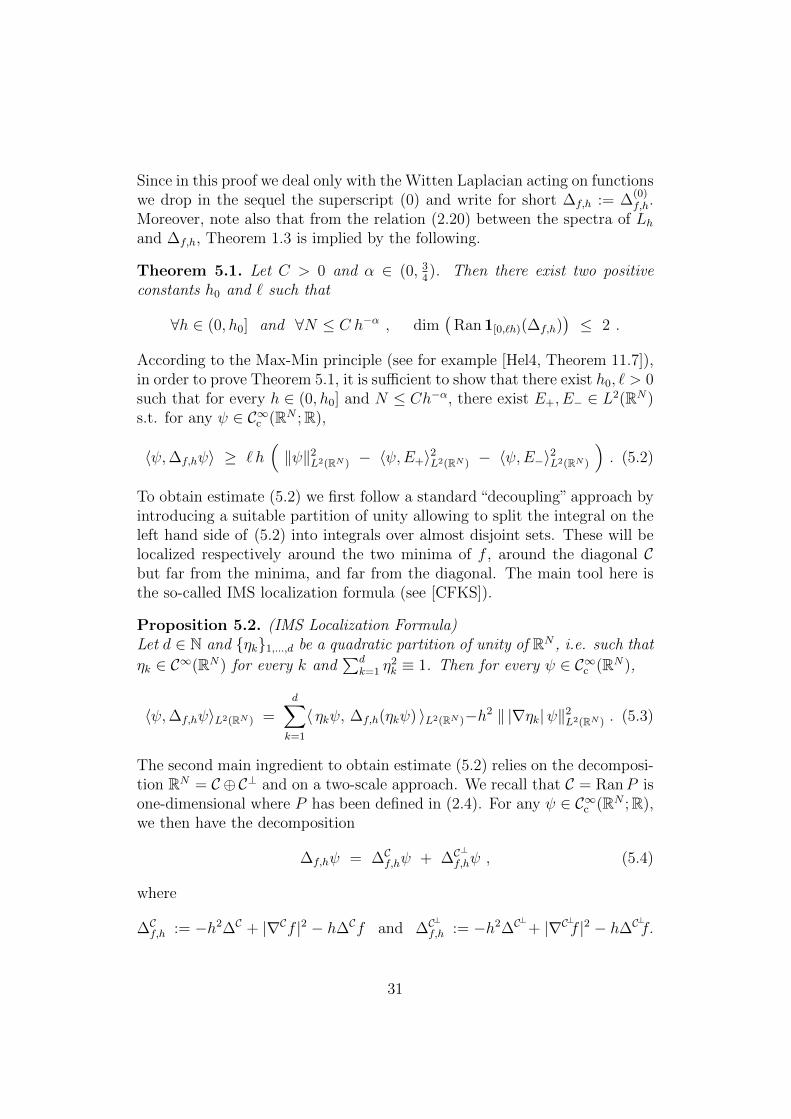
Since in this proof we deal only with the Witten Laplacian acting on functionswe drop in the sequel the superscript (0) and write for short ∆f,h := ∆

(0)f,h.

Moreover, note also that from the relation (2.20) between the spectra of Lhand ∆f,h, Theorem 1.3 is implied by the following.

Theorem 5.1. Let C > 0 and α ∈ (0, 34). Then there exist two positive

constants h0 and ` such that

∀h ∈ (0, h0] and ∀N ≤ C h−α , dim(

Ran 1[0,`h)(∆f,h))≤ 2 .

According to the Max-Min principle (see for example [Hel4, Theorem 11.7]),in order to prove Theorem 5.1, it is sufficient to show that there exist h0, ` > 0such that for every h ∈ (0, h0] and N ≤ Ch−α, there exist E+, E− ∈ L2(RN)s.t. for any ψ ∈ C∞c (RN ;R),

〈ψ,∆f,hψ〉 ≥ ` h(‖ψ‖2

L2(RN ) − 〈ψ,E+〉2L2(RN ) − 〈ψ,E−〉2L2(RN )

). (5.2)

To obtain estimate (5.2) we first follow a standard “decoupling” approach byintroducing a suitable partition of unity allowing to split the integral on theleft hand side of (5.2) into integrals over almost disjoint sets. These will belocalized respectively around the two minima of f , around the diagonal Cbut far from the minima, and far from the diagonal. The main tool here isthe so-called IMS localization formula (see [CFKS]).

Proposition 5.2. (IMS Localization Formula)Let d ∈ N and ηk1,...,d be a quadratic partition of unity of RN , i.e. such that

ηk ∈ C∞(RN) for every k and∑d

k=1 η2k ≡ 1. Then for every ψ ∈ C∞c (RN),

〈ψ,∆f,hψ〉L2(RN ) =d∑

k=1

〈 ηkψ, ∆f,h(ηkψ) 〉L2(RN )−h2 ‖ |∇ηk|ψ‖2L2(RN ) . (5.3)

The second main ingredient to obtain estimate (5.2) relies on the decomposi-tion RN = C ⊕C⊥ and on a two-scale approach. We recall that C = RanP isone-dimensional where P has been defined in (2.4). For any ψ ∈ C∞c (RN ;R),we then have the decomposition

∆f,hψ = ∆Cf,hψ + ∆C⊥

f,hψ , (5.4)

where

∆Cf,h := −h2∆C + |∇Cf |2 − h∆Cf and ∆C⊥

f,h := −h2∆C⊥

+ |∇C⊥f |2 − h∆C⊥f.

31

Here, the superscripts C, C⊥ on a differential operator mean that differenti-ation is restricted to the corresponding subspace. Thus, chosing some nor-malized coordinate y0 on C and orthonormal coordinates (z1, . . . , zN−1) onC⊥ we have for example for every ψ ∈ C∞(RN),

∆Cψ =∂2ψ

∂y20

, ∆C⊥ψ =

N−1∑k=1

∂2ψ

∂z2k

.

Note in particular that the orthogonal decomposition

x = Px + P⊥x = x0

(1√N, . . . ,

1√N

)+ P⊥x

leads to

∇Cf(x) =1

2

√N

N∑k=1

( x0√N

+ P⊥x)3

k− 1

2x0 (5.5)

and

∆Cf(x) =1

2

(3x2

0 + 3‖P⊥x‖2 − 1). (5.6)

Given ψ : RN → R and y ∈ C, we denote by ψy the partial application

ψy : z ∈ C⊥ 7−→ ψ(y + z) (5.7)

and hence satisfying ψy(C⊥) = ψ(x ∈ RN : Px = y).Roughly speaking, we shall exploit decomposition (5.4) as follows. Away

from the diagonal, we use ∆Cf,h ≥ 0 and exploit (2.8), namely that HessC⊥

is strictly convex, uniformly in x and N ∈ N. This leads for every fixedy ∈ C to spectral gap lower bounds for the operator ψy 7→ (∆C

⊥

f,hψ)y (seeLemma 5.3 below). The dependence on y of these estimates is controlled inLemma 5.4 below. Around the diagonal C but away from the critical pointswe use ∆C

⊥

f,h ≥ 0 and work with ∆Cf,h, which, when restricted to sufficientlysmall neighbourhoods of C, behaves essentially like the 1-dimensional WittenLaplacian associated with f |C (see the discussion after (5.34) below). Aroundthe minima J+ and J− we work directly with ∆f,h. Here we use that therestriction of f to sufficiently small neighbourhoods around J+ and J− isuniformly convex, and thus, locally, good spectral gap lower bounds can beobtained (see Lemma 5.5 and Proposition 5.7 below).

The rest of the section is organized as follows. In Subsection 5.1 we makeprecise and prove some aforementioned preliminary results which are neededfor the proof of Theorem 5.1. In Subsection 5.2 we introduce a suitablequadratic partition of unity of RN and give the proof of Theorem 5.1.

32

5.1 Preliminary estimates

In the sequel we write y and z to denote generic elements of C and C⊥respectively and dy, dz for the Lebesgue measures on C and C⊥. We recallalso the notation defined in (5.7).

The combination of the following two lemmata allows to control the quadraticform 〈∆f,hψ, ψ〉L2(RN ) away from the diagonal C.

Lemma 5.3 (Poincare inequality for fixed y ∈ C). The following inequalityholds true for every h > 0, N ∈ N, ψ ∈ C∞c (RN) and y ∈ C:

〈ψy, (∆C⊥

f,hψ)y 〉L2(C⊥) ≥ h (µ−1)(‖ψy‖2

L2(C⊥) − 〈ψy, Ey 〉2L2(C⊥)

), (5.8)

where E : RN → R is given by

E(x) :=e−

f(x)h( ∫

C⊥ e−2

f(Px+z)h dz

) 12

. (5.9)

Proof. Note that (5.8) is equivalent to the inequality∫C⊥‖∇C⊥(E−1ψ)y‖2E2

ydz ≥µ− 1

h

(∫C⊥

(E−1ψ)2yE

2ydz −

(∫C⊥

(E−1ψ)yE2ydz)2)

which follows from the uniform convexity estimate

1

hHessC

⊥2f(x) =

1

hHessC

⊥V (√Nx) ≥ µ− 1

h

implied by (2.8), and standard criteria for the spectral gap of strictly log-concave measures (see for example [Led, Corollary 11.4] or the already usedBakry-Emery criterion of Proposition 3.4 which gives an even stronger re-sult).

Note that by integrating the relation (5.8) of Lemma 5.3 in y and usingthe Cauchy-Schwarz inequality, we get that for every h > 0, N ∈ N andψ ∈ C∞c (RN),

〈ψ, ∆C⊥

f,hψ 〉L2(RN ) ≥ h(µ− 1) ‖ψ‖2L2(RN )

(1− sup

y∈suppψ

∫suppψy

E2y(z) dz

).

(5.10)In order to fully exploit Estimate (5.10), we need a control on the integralappearing on its right hand side when ψ is localised far from the diagonal.The following rough tail estimate will be enough for our purposes.

33

Lemma 5.4 (Concentration Lemma).Let h, Rh and ρ be three positive numbers. Then there exist h0 > 0 and γ > 0such that for every h ∈ (0, h0] and N ∈ N, the function E defined in (5.9)satisfies

sup‖y‖≤ρ

∫‖z‖≥Rh

E2y(z) dz ≤ minγ e−

R2hγh , 1 , (5.11)

and

supy∈C

∫‖z‖≥Rh

E2y(z) dz ≤ mineγN e−

R2hγh , 1 . (5.12)

Proof. For every τ ∈ R+, h > 0, N ∈ N and y ∈ C, we have the upper bound∫‖z‖≥Rh

E2y(z) dz ≤ e−τ

R2hh

∫C⊥eτ‖z‖2h E2

y(z) dz . (5.13)

To estimate the integral on the right hand side of (5.13), we shall use thefollowing two bounds on f :

2f(x) − 2f(Px) ≤ 3N

4‖P⊥x‖4

4 +1

2〈P⊥x ,

(K−1+4‖Px‖2

)P⊥x 〉 , (5.14)

and

2f(x) − 2f(Px) ≥ 1

2〈P⊥x , (K − 1 + ‖Px‖2)P⊥x 〉 . (5.15)

Estimate (5.15) follows immediately from the definition (5.1) of f and fromthe inequalities

N

4‖x‖4

4 ≥1

4‖x‖4 =

1

4(‖Px‖2 + ‖P⊥x‖2)2 ≥ 1

2‖Px‖2 ‖P⊥x‖2 +

1

4‖Px‖4

together with ‖Px‖4 = N‖Px‖44 = N2x4. To see (5.14), note first that from

the definition of f ,

2f(x) − 2f(Px) =N

4‖P⊥x‖4

4 + NxN∑k=1

(P⊥x)3k

+1

2〈P⊥x,

(K − 1 + 3‖Px‖2

)P⊥x 〉 ,

so (5.14) is a consequence of the elementary inequalities

∣∣Nx N∑k=1

(P⊥x)3k

∣∣ ≤ √N‖Px‖‖P⊥x‖24‖P⊥x‖ ≤

1

2‖Px‖2‖P⊥x‖2 +

N

2‖P⊥x‖4

4 .

34

From (5.13), together with (5.14), (5.15) and computations of Gaussian in-tegrals, we obtain for every h > 0, N ∈ N and for every τ ∈ (0, µ−1

2),∫

‖z‖≥RhE2y(z) dz ≤ e−τ

R2hh

Θ(τ,N, y)

1− ε(h,N, y), (5.16)

where

Θ(τ,N, y) :=( det(K − 1 + 4‖y‖2)

det(K − 1 + ‖y‖2 − 2τ)

) 12, (5.17)

and

ε(h,N, y) :=

(det(K − 1 + 4‖y‖2)

) 12

(2πh)N2

∫C⊥

(1− e−

3N‖z‖444h

)e−〈z,(K−1+4‖y‖2)z〉

2h dz.

As in the proof of Proposition 3.13, we use the simple estimate

|ε(h,N, y)| ≤(

det(K − 1 + 4‖y‖2)) 1

2

(2πh)N2

1

4h

∫C⊥

3N‖z‖44 e− 〈z,(K−1+4‖y‖2)z〉

2h dz ,

and conclude, by applying a straightforward modification of Lemma 2.2, thatthere exists a constant C > 0 such that for every N ∈ N, h ∈ (0, 1] andy ∈ RN ,

|ε(h,N, y)| ≤ C h . (5.18)

In order to control Θ(τ,N, y), we fix τ ∈ (0, 38(µ − 1)) so that Θ(τ,N, y)

increases with ‖y‖ (for any fixed N), and observe that, arguing as in theproof of Lemma 2.4, for every ρ > 0 there exists a constant C > 0 such that

∀N ∈ N , sup‖y‖≤ρ

Θ(τ,N, y) ≤ C . (5.19)

If y is not constrained to a compact set, we get the existence of a constantC > 0 such that for every N ∈ N, y ∈ RN ,

Θ(τ,N, y) ≤ 4N2 ≤ eCN . (5.20)

Thus, from (5.16), taking h0 and γ−1 sufficiently small, one obtains (5.11)according to (5.18), (5.19) and one obtains (5.12) according to (5.18), (5.20).

The following lemma shows the existence of a suitable neighbourhood ofthe minimum J+ on which f is uniformly convex. Note that by symmetryarguments, the analogous statement holds with J− instead of J+.

35

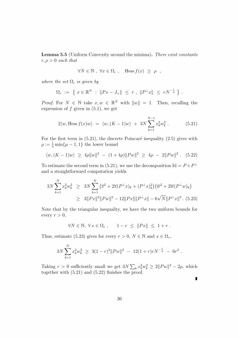
Lemma 5.5 (Uniform Convexity around the minima). There exist constantsr, ρ > 0 such that

∀N ∈ N , ∀x ∈ Ωr , Hess f(x) ≥ ρ ,

where the set Ωr is given by

Ωr :=x ∈ RN : ‖Px− J+‖ ≤ r , ‖P⊥x‖ ≤ rN−

14

.

Proof. For N ∈ N take x,w ∈ RN with ‖w‖ = 1. Then, recalling theexpression of f given in (5.1), we get

2〈w,Hess f(x)w〉 = 〈w, (K − 1)w〉 + 3NN−1∑k=1

x2kw

2k . (5.21)

For the first term in (5.21), the discrete Poincare inequality (2.5) gives withρ := 1

4minµ− 1, 1 the lower bound

〈w, (K − 1)w〉 ≥ 4ρ‖w‖2 − (1 + 4ρ)‖Pw‖2 ≥ 4ρ − 2‖Pw‖2 . (5.22)

To estimate the second term in (5.21), we use the decomposition Id = P+P⊥

and a straightforward computation yields

3NN∑k=1

x2kw

2k ≥ 3N

N∑k=1

(x2 + 2x(P⊥x)k + (P⊥x)2

k

)(w2 + 2w(P⊥w)k

)≥ 3‖Px‖2‖Pw‖2 − 12‖Px‖‖P⊥x‖ − 6

√N‖P⊥x‖2 . (5.23)

Note that by the triangular inequality, we have the two uniform bounds forevery r > 0,

∀N ∈ N, ∀x ∈ Ωr , 1− r ≤ ‖Px‖ ≤ 1 + r .

Thus, estimate (5.23) gives for every r > 0, N ∈ N and x ∈ Ωr,

3NN∑k=1

x2kw

2k ≥ 3(1− r)2‖Pw‖2 − 12(1 + r)rN−

14 − 6r2 .

Taking r > 0 sufficiently small we get 3N∑

k x2kw

2k ≥ 2‖Pw‖2 − 2ρ, which

together with (5.21) and (5.22) finishes the proof.

36

The preceding Lemma 5.5 is used to establish the localized spectral gapestimate of Proposition 5.7 below. As in the proof of Lemma 5.3, we argue bymeans of standard results for strictly log-concave measures. To reduce to thestandard situation, we use the following general result on convex extensions,for which we provide a proof for the sake of completeness.

Lemma 5.6. Fix d ∈ N. Let ϕ ∈ C∞(Rd) and A be a compact and convexsubset of Rd such that

∃ ε > 0 , ∃C > 0 s.t. Hessϕ ≥ C on Aε := x+ y ; x ∈ A , ‖y‖ ≤ ε .

Then there exists ϕ ∈ C∞(Rd) such that

∀x ∈ A , ϕ(x) = ϕ(x) and ∀x ∈ Rd , Hess ϕ(x) ≥ C .

Proof. The proof consists in smoothly cutting ϕ outside A and adding afunction g vanishing on A and sufficiently convex outside A. To easily con-struct such a function g it is convenient to reduce to radial cut-off’s as follows(see [Yan]): first, since A is convex and compact, Aε \ A ε

2is compact and

there exist ` ∈ N, (xi)i∈1,...,` ⊂ (RN)` and (ri)i∈1,...,` ⊂ (0,∞)` such that,denoting by B(xi, ri) the closed ball of radius ri centered at xi,

A ⊂ ∩`i=1B(xi, ri) ⊂ A ε2⊂ Aε . (5.24)

We shall consider θ ∈ C∞(R) defined by

θ(t) :=

0 if t ∈ (−∞, 1]

t2e−1t−1 if t ∈ (1,+∞) .

This function is strictly increasing on (1,+∞), as well as t 7→ θ′(t)t

, since wehave for any t > 1,

θ′(t) =

(2t+

t2

(t− 1)2

)e−

1t−1 and

(θ′(t)

t

)′=

t2 − 3t+ 3

(t− 1)4e−

1t−1 .

Moreover notice that Hess(x 7→ θ(‖x‖)

)is given by

Hess(x 7→ θ(‖x‖)

)=

θ′(‖x‖)‖x‖

Id +1

‖x‖

(θ′(t)

t

)′t=‖x‖

(xixj

)1≤i,j≤N ,

and so is positive definite for ‖x‖ > 1 (and zero for ‖x‖ ≤ 1). We then define

g(x) :=∑i=1

θ

(‖x− xi‖

ri

).

37

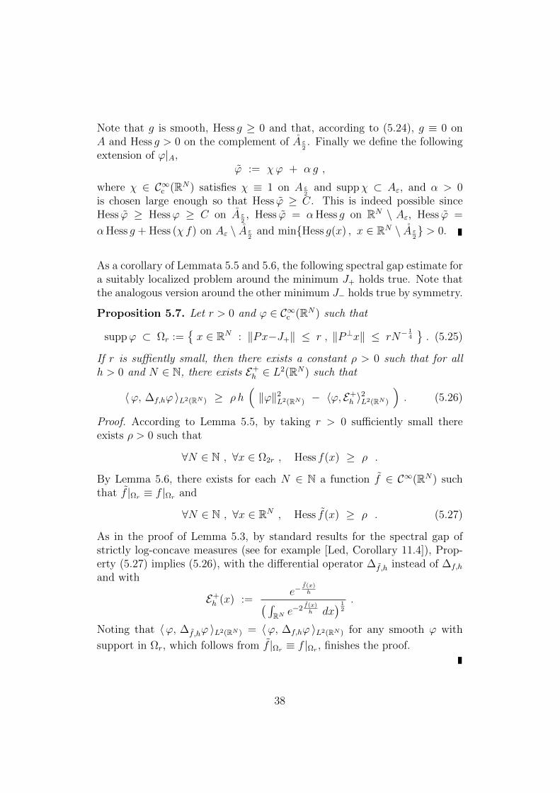
Note that g is smooth, Hess g ≥ 0 and that, according to (5.24), g ≡ 0 onA and Hess g > 0 on the complement of A ε

2. Finally we define the following

extension of ϕ|A,ϕ := χϕ + α g ,

where χ ∈ C∞c (RN) satisfies χ ≡ 1 on A ε2

and suppχ ⊂ Aε, and α > 0is chosen large enough so that Hess ϕ ≥ C. This is indeed possible sinceHess ϕ ≥ Hessϕ ≥ C on A ε

2, Hess ϕ = αHess g on RN \ Aε, Hess ϕ =

αHess g + Hess (χ f) on Aε \ A ε2

and minHess g(x) , x ∈ RN \ A ε2 > 0.

As a corollary of Lemmata 5.5 and 5.6, the following spectral gap estimate fora suitably localized problem around the minimum J+ holds true. Note thatthe analogous version around the other minimum J− holds true by symmetry.

Proposition 5.7. Let r > 0 and ϕ ∈ C∞c (RN) such that

suppϕ ⊂ Ωr :=x ∈ RN : ‖Px−J+‖ ≤ r , ‖P⊥x‖ ≤ rN−

14

. (5.25)

If r is suffiently small, then there exists a constant ρ > 0 such that for allh > 0 and N ∈ N, there exists E+

h ∈ L2(RN) such that

〈ϕ, ∆f,hϕ 〉L2(RN ) ≥ ρ h(‖ϕ‖2

L2(RN ) − 〈ϕ, E+h 〉

2L2(RN )

). (5.26)

Proof. According to Lemma 5.5, by taking r > 0 sufficiently small thereexists ρ > 0 such that

∀N ∈ N , ∀x ∈ Ω2r , Hess f(x) ≥ ρ .

By Lemma 5.6, there exists for each N ∈ N a function f ∈ C∞(RN) suchthat f |Ωr ≡ f |Ωr and

∀N ∈ N , ∀x ∈ RN , Hess f(x) ≥ ρ . (5.27)

As in the proof of Lemma 5.3, by standard results for the spectral gap ofstrictly log-concave measures (see for example [Led, Corollary 11.4]), Prop-erty (5.27) implies (5.26), with the differential operator ∆f ,h instead of ∆f,h

and with

E+h (x) :=

e−f(x)h( ∫

RN e−2

f(x)h dx

) 12

.

Noting that 〈ϕ, ∆f ,hϕ 〉L2(RN ) = 〈ϕ, ∆f,hϕ 〉L2(RN ) for any smooth ϕ with

support in Ωr, which follows from f |Ωr ≡ f |Ωr , finishes the proof.

38

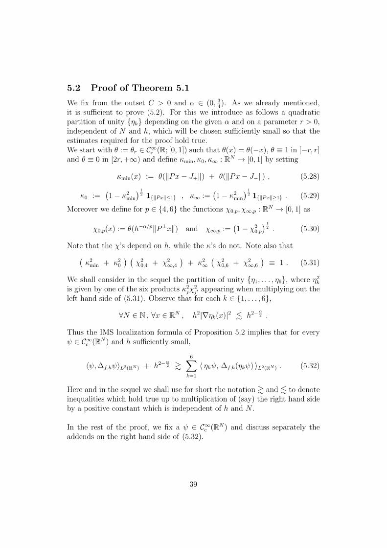
5.2 Proof of Theorem 5.1

We fix from the outset C > 0 and α ∈ (0, 34). As we already mentioned,

it is sufficient to prove (5.2). For this we introduce as follows a quadraticpartition of unity ηk depending on the given α and on a parameter r > 0,independent of N and h, which will be chosen sufficiently small so that theestimates required for the proof hold true.We start with θ := θr ∈ C∞c (R; [0, 1]) such that θ(x) = θ(−x), θ ≡ 1 in [−r, r]and θ ≡ 0 in [2r,+∞) and define κmin, κ0, κ∞ : RN → [0, 1] by setting

κmin(x) := θ(‖Px− J+‖) + θ(‖Px− J−‖) , (5.28)

κ0 :=(1− κ2

min

) 12 1‖Px‖≤1 , κ∞ :=

(1− κ2

min

) 12 1‖Px‖≥1 . (5.29)

Moreover we define for p ∈ 4, 6 the functions χ0,p, χ∞,p : RN → [0, 1] as

χ0,p(x) := θ(h−α/p‖P⊥x‖) and χ∞,p :=(1− χ2

0,p

) 12 . (5.30)

Note that the χ’s depend on h, while the κ’s do not. Note also that(κ2

min + κ20

) (χ2

0,4 + χ2∞,4

)+ κ2

∞(χ2

0,6 + χ2∞,6

)≡ 1 . (5.31)

We shall consider in the sequel the partition of unity η1, . . . , η6, where η2k

is given by one of the six products κ2jχ

2j′ appearing when multiplying out the

left hand side of (5.31). Observe that for each k ∈ 1, . . . , 6,

∀N ∈ N , ∀x ∈ RN , h2|∇ηk(x)|2 . h2−α2 .

Thus the IMS localization formula of Proposition 5.2 implies that for everyψ ∈ C∞c (RN) and h sufficiently small,

〈ψ,∆f,hψ〉L2(RN ) + h2−α2 &

6∑k=1

〈 ηkψ, ∆f,h(ηkψ) 〉L2(RN ) . (5.32)

Here and in the sequel we shall use for short the notation & and . to denoteinequalities which hold true up to multiplication of (say) the right hand sideby a positive constant which is independent of h and N .

In the rest of the proof, we fix a ψ ∈ C∞c (RN) and discuss separately theaddends on the right hand side of (5.32).

39

Analysis around the diagonal

a) Analysis on supp(κmin χ0,4

): According to the definitions given in (5.28)

and (5.30), we have for every h > 0 and N ∈ N such that N ≤ Ch−α,

supp(ψ κmin χ0,4 ) ⊂ Ω+,r ∪ Ω−,r ,

where Ω±,r :=x ∈ RN : ‖Px± J+‖ ≤ 2r , ‖P⊥x‖ ≤ 2rC

14N−

14

.

Then it follows from Proposition 5.7 (and its analogous version around J−)that, chosing r sufficiently small, for all h > 0 and N ≤ Ch−α there existE+h , E

−h ∈ L2(RN) such that, denoting for short ϕ := κminχ0,4 ψ,

〈ϕ, ∆f,h ϕ 〉L2(RN ) & h(‖ϕ‖2

L2(RN ) − 〈ϕ, E+h 〉

2L2(RN ) − 〈ϕ, E

−h 〉

2L2(RN )

). (5.33)

b) Analysis on supp(κ2

0 χ20,4 + κ2

∞ χ20,6

): Here we shall use that, in the sense

of quadratic forms,

∆f,h ≥ ∆Cf,h ≥ |∇Cf |2 − h∆Cf . (5.34)

The final estimate (5.40) given below follows then by elementary inequalitieswhich we spell out for completeness. Note first that the definitions (5.29)and (5.30) imply in particular that for every h > 0 and N ∈ N,

supp(κ2

0 χ20,4 + κ2

∞ χ20,6

)⊂ Ω0 ∪ Ω , (5.35)

where Ω and Ω0 are defined as

Ω :=x ∈ RN : ‖Px− J±‖ ≥ r , ‖Px‖ ≥ r , ‖P⊥x‖ ≤ 2rh

α6

,

andΩ0 :=

x ∈ RN : ‖Px‖ ≤ r , ‖P⊥x‖ ≤ 2rh

α6

.

On Ω0 one can immediately give a lower bound for the right hand sidein (5.34). Indeed, chosing r sufficiently small, we have from (5.6) for ev-ery x ∈ Ω0, h ∈ (0, 1], and N ∈ N,

|∇Cf |2 − h∆Cf ≥ − h∆Cf =h

2(1− 3x2

0 − 3‖P⊥x‖2) ≥ h

4. (5.36)

To deal with Ω, we develop the expression of ∇Cf(x) given in (5.5),

∇Cf(x) =1

2x3

0 −1

2x0 +

3

2x0‖P⊥x‖2 +

1

2

√N

N∑k=1

(P⊥x)3k ,

40

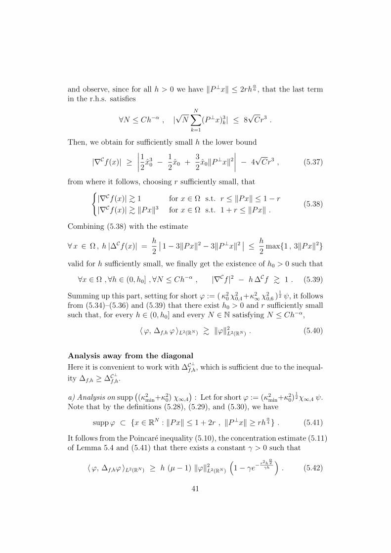
and observe, since for all h > 0 we have ‖P⊥x‖ ≤ 2rhα6 , that the last term

in the r.h.s. satisfies

∀N ≤ Ch−α , |√N

N∑k=1

(P⊥x)3k| ≤ 8

√Cr3 .

Then, we obtain for sufficiently small h the lower bound

|∇Cf(x)| ≥∣∣∣∣12 x3

0 −1

2x0 +

3

2x0‖P⊥x‖2

∣∣∣∣ − 4√Cr3 , (5.37)

from where it follows, choosing r sufficiently small, that|∇Cf(x)| & 1 for x ∈ Ω s.t. r ≤ ‖Px‖ ≤ 1− r|∇Cf(x)| & ‖Px‖3 for x ∈ Ω s.t. 1 + r ≤ ‖Px‖ .

(5.38)

Combining (5.38) with the estimate

∀x ∈ Ω , h |∆Cf(x)| =h

2

∣∣ 1− 3‖Px‖2 − 3‖P⊥x‖2∣∣ ≤ h

2max1 , 3‖Px‖2

valid for h sufficiently small, we finally get the existence of h0 > 0 such that

∀x ∈ Ω ,∀h ∈ (0, h0] ,∀N ≤ Ch−α , |∇Cf |2 − h∆Cf & 1 . (5.39)

Summing up this part, setting for short ϕ := (κ20 χ

20,4 +κ2

∞ χ20,6 )

12 ψ, it follows

from (5.34)–(5.36) and (5.39) that there exist h0 > 0 and r sufficiently smallsuch that, for every h ∈ (0, h0] and every N ∈ N satisfying N ≤ Ch−α,

〈ϕ, ∆f,h ϕ 〉L2(RN ) & ‖ϕ‖2L2(RN ) . (5.40)

Analysis away from the diagonal

Here it is convenient to work with ∆C⊥

f,h, which is sufficient due to the inequal-

ity ∆f,h ≥ ∆C⊥

f,h.

a) Analysis on supp((κ2

min+κ20) χ∞,4

): Let for short ϕ := (κ2

min+κ20)

12χ∞,4 ψ.

Note that by the definitions (5.28), (5.29), and (5.30), we have

suppϕ ⊂ x ∈ RN : ‖Px‖ ≤ 1 + 2r , ‖P⊥x‖ ≥ rhα4 . (5.41)

It follows from the Poincare inequality (5.10), the concentration estimate (5.11)of Lemma 5.4 and (5.41) that there exists a constant γ > 0 such that

〈ϕ, ∆f,hϕ 〉L2(RN ) ≥ h (µ− 1) ‖ϕ‖2L2(RN )

(1− γe−

r2hα2

γh

). (5.42)

41

Since 0 < α < 34, estimate (5.42) implies that there exists h0 > 0 such that

∀h ∈ (0, h0] , ∀N ∈ N , 〈ϕ, ∆f,hϕ 〉L2(RN ) ≥ h(µ− 1)

2‖ϕ‖2

L2(RN ) . (5.43)

b) Analysis on supp(κ∞ χ∞,6

): Let ϕ := κ∞ χ∞,6 ψ. By the definitions (5.29)

and (5.30), we have

suppϕ ⊂ x ∈ RN : ‖P⊥x‖ ≥ rhα6 . (5.44)

As for the point a) above, we use the Poincare inequality (5.10) but we canonly use here the concentration estimate (5.12) of Lemma 5.4 since suppψ isarbitrary. This leads to the existence of a constant γ > 0 such that

〈ϕ, ∆f,hϕ 〉L2(RN ) ≥ h(µ− 1) ‖ϕ‖2L2(RN )

(1− eγN−

r2hα3

γh

). (5.45)

Since 0 < α < 34, estimate (5.45) implies that there exists h0 > 0 such that

∀h ∈ (0, h0] , ∀N ≤ Ch−α , 〈ϕ, ∆f,hϕ 〉L2(RN ) ≥ h(µ− 1)

2‖ϕ‖2

L2(RN ). (5.46)

End of the proof

Chosing the parameter r > 0 of the partition of unity ηk sufficiently smalland putting together (5.32), (5.33), (5.40), (5.43), and (5.46), we obtainestimate (5.2) with E± := E±h κmin χ0,4.

AcknowledgementsThis work was supported by the NOSEVOL ANR 2011 BS01019 01 and theEuropean Research Council under the European Union’s Seventh FrameworkProgramme (FP/2007-2013) / ERC Grant Agreement number 614492. Theauthors’ collaboration was initiated thanks to a research visit to Paris-SudUniversity of the first author, then founded by the Department of Math-ematics of the University of Rome La Sapienza, and completed during a“Delegation INRIA” of the second author at CERMICS.

Both authors thank Bernard Helffer and Nils Berglund for various discussions,Anton Bovier for pointing to the problem, and Tony Lelievre for offering ex-cellent working conditions at CERMICS.

42

References

[BaMø] V. Bach and J. S. Møller. Correlation at low temperature: I. Expo-nential decay. J. Funct. Anal. 203, no. 1, pp. 93–148 (2003).

[BaEm] D. Bakry and M. Emery. Diffusions hypercontractives. Sem. Probab.XIX, Lecture Notes in Math. 1123, pp. 177–206, Springer (1985).

[BGL] D. Bakry, I. Gentil, and M. Ledoux. Analysis and geometry of Markovdiffusion operators. Grund. der Math. Wiss. 348, Springer (2014).

[Bar] F. Barret. Sharp asymptotics of metastable transition times for onedimensional SPDEs. Ann. IHP Proba. Stat. 51, no. 1, pp. 129–166(2015).

[BBM] F. Barret, A. Bovier, and S. Meleard. Uniform estimates formetastable transitions in a coupled bistable system. Electron. J.Probab., 15, no. 12, pp. 323–345 (2010).

[BFG1] N. Berglund, B. Fernandez, and B. Gentz. Metastability in interact-ing nonlinear stochastic differential equations: I. From weak coupling tosynchronization. Nonlinearity 20, no. 11, pp. 2551–2581 (2007).

[BFG2] N. Berglund, B. Fernandez, and B. Gentz. Metastability in interact-ing nonlinear stochastic differential equations: II. Large-N behaviour.Nonlinearity 20, no. 11, pp. 2583–2614 (2007).

[BeGe] N. Berglund and B. Gentz. Sharp estimates for metastable lifetimesin parabolic SPDEs: Kramers’ law and beyond. Electron. J. Probab.,18, no. 24, pp. 1–58 (2013).

[BoHe1] T. Bodineau and B. Helffer. The log-Sobolev inequality for un-bounded spin systems. J. Funct. Anal. 166, no. 1, pp. 168–178 (1999).

[BoHe2] T. Bodineau and B. Helffer. Correlations, spectral gap and log-Sobolev inequalities for unbounded spins systems. Differential equationsand mathematical physics, AMS/IP Stud. Adv. Math., 16, pp. 51–66(2000).

[BHM] J.-F. Bony, F. Herau, and L. Michel. Tunnel effect for semiclassicalrandom walks. Anal. PDE 8, no. 2, pp. 289–332 (2015).

[BEGK] A. Bovier, M. Eckhoff, V. Gayrard, and M. Klein. Metastabilityin reversible diffusion processes I: Sharp asymptotics for capacities andexit times. JEMS 6(4), pp. 399–424 (2004).

43

[BGK] A. Bovier, V. Gayrard, and M. Klein. Metastability in reversiblediffusion processes II: Precise asymptotics for small eigenvalues. JEMS7(1), pp. 69–99 (2004).

[BDP] S. Brassesco, A. De Masi, and E. Presutti. Brownian fluctuations ofthe interface in the D=1 Ginzburg-Landau equation with noise. Ann.IHP Proba. Stat. 31, no. 1, pp. 81–118 (1995).

[CFKS] H. L. Cycon, R. G. Froese, W. Kirsch, and B. Simon. Schrodingeroperators with application to quantum mechanics and global geometry.Text and Monographs in Physics, Springer–Verlag (1987).

[Dap] G. Da Prato. An Introduction to Infinite Dimensional Analysis. Uni-versitext, Springer–Verlag (2006).

[DaZa] G. Da Prato and J. Zabczyk. Stochastic equations in infinite dimen-sions. Second edition. Encyclopedia of Mathematics and its Applica-tions, 152, Cambridge University Press (2014).

[Dig] G. Di Gesu. Semiclassical spectral analysis of discrete Witten Lapla-cians. PhD thesis, available on https://publishup.uni-potsdam.de/

opus4-ubp/frontdoor/index/index/docId/6287 (2013).

[FaJo] W. Faris and G. Jona-Lasinio. Large fluctuations for a nonlinear heatequation with noise. J. Phys. A 15, no. 10, pp. 3025–3055 (1982).

[FrWe] M. I. Freidlin and A. D. Wentzell. Random perturbations of dynamicalsystems. Third edition. Grund. der Math. Wiss. 260, Springer (2012).

[Fun] T. Funaki. Random motion of strings and related stochastic evolutionequations. Nagoya Math. J. 89, pp. 129–193 (1983).

[GlJa] J. Glimm and A. Jaffe. Quantum physics. A functional integral pointof view. Second edition. Springer–Verlag (1987).

[GoMa] B. Goldys and B. Maslowski. Uniform exponential ergodicity ofstochastic dissipative systems. Czechoslovak Math. J. 51 (126), no. 4,pp. 745–762 (2001).

[Hai1] M. Hairer. Exponential mixing properties of stochastic PDEs throughasymptotic coupling. Probab. Theory Relat. Fields 124, no. 3, pp. 345–380 (2002).

[Hai2] M. Hairer, An introduction to stochastic PDEs. Lecture Notes, avail-able on http://www.hairer.org/notes/SPDEs.pdf (2009).

44

[Hel1] B. Helffer. Semiclassical analysis for Schrodinger operators, Laplaceintegrals and transfer operators in large dimension: an introduction.DEA course at Paris-Sud University, available on http://www.math.

u-psud.fr/~helffer/ (1995).

[Hel2] B. Helffer. Remarks on the decay of correlations and Witten Lapla-cians – the Brascamp-Lieb inequality and semiclassical limit. J. Func-tional Analysis 155, pp. 571–586 (1998).

[Hel3] B. Helffer. Semiclassical Analysis, Witten Laplacians, and StatisticalMechanics. Series in Partial Differential Equations and Applications, 1.World Scientific (2002).

[Hel4] B. Helffer. Spectral theory and its applications. Cambridge Studies inAdvanced Mathematics, 139. Cambridge University Press (2013).

[HKN] B. Helffer, M. Klein, and F. Nier. Quantitative analysis of metasta-bility in reversible diffusion processes via a Witten complex approach.Matematica Contemporanea 26, pp. 41–85 (2004).

[HeNi1] B. Helffer and F. Nier. Quantitative analysis of metastability inreversible diffusion processes via a Witten complex approach: the casewith boundary. Memoire 105, Societe Mathematique de France (2006).

[HeNi2] B. Helffer and F. Nier. Hypoelliptic estimates and spectral theoryfor Fokker-Planck operators and Witten Laplacians. Lecture Notes inMathematics 1862, Springer–Verlag (2005).

[HeSj] B. Helffer and J. Sjostrand. Puits multiples en limite semi-classique IV-Etude du complexe de Witten -. Comm. Partial Differential Equations10 (3), pp. 245–340 (1985).

[HoSt] R. Holley and D. Stroock. Logarithmic Sobolev inequalities andstochastic Ising models. J. Statist. Phys. 46, no. 5–6, pp. 1159–1194(1987).

[Joh] J. Johnsen. On the spectral properties of Witten Laplacians, their rangeprojections and Brascamp-Lieb’s inequality. Integral Equations Opera-tor Theory 36 (3), pp. 288–324 (2000).

[JMS] G. Jona-Lasinio, F. Martinelli, and E. Scoppola. New approach to thesemiclassical limit of quantum mechanics. I. Multiple tunnelings in onedimension. Comm. Math. Phys. 80, no. 2, pp. 223–254 (1981).

45

[Led] M. Ledoux, Logarithmic Sobolev inequalities for unbounded spinsystmes revisited. Sem. Probab. XXXV, Lecture Notes in Math. 1755,pp. 167–194 Springer (2001).

[KuTa] J. Kurchan and S. Tanase-Nicola. Metastable states, transitions,basins and borders at finite temperatures. J. Statist. Phys. 116, no. 5-6,pp. 1201–1245 (2004).

[Lep] D. Le Peutrec. Small eigenvalues of the Neumann realization of thesemiclassical Witten Laplacian. Ann. de la Faculte des Sciences deToulouse, Vol. 19, no. 3–4, pp. 735–809 (2010).

[LeNi] T. Lelievre and F. Nier. Low temperature asymptotics for quasi-stationary distributions in a bounded domain. Anal. PDE 8, no. 3,pp. 561–628 (2015).

[MaMø] O. Matte and J. S. Møller. On the spectrum of semi-classical Witten-Laplacians and Schrodinger operators in large dimension. J. Funct. Anal.220, no. 2, pp. 243–264 (2005).

[MeSc] G. Menz and A. Schlichting. Poincare and logarithmic Sobolev in-equalities by decomposition of the energy landscape. Ann. Probab. 42,no. 5, pp. 1809–1884 (2014).

[Mic] L. Miclo. On hyperboundedness and spectrum of Markov operators.Invent. Math. 200, no. 1, pp. 311–343 (2015).

[KORV] R. V. Kohn, F. Otto, M. G. Reznikoff, and E. Vanden-Eijnden.Action minimization and sharp-interface limits for the stochastic Allen-Cahn equation. Comm. Pure Appl. Math. 60, no. 3, pp. 393–438 (2007).

[OWW] F. Otto, H. Weber, and M. Westdickenberg. Invariant measure ofthe stochastic Allen-Cahn equation: the regime of small noise and largesystem size. Electron. J. Probab. 19, no. 23, pp. 1–76 (2014).

[ReVe] M. G. Reznikoff and E. Vanden-Eijnden. Invariant measures ofstochastic partial differential equations and conditioned diffusions.C. R. Math. Acad. Sci. Paris 340, no. 4, pp. 305–308 (2005).

[Roy] G. Royer. An initiation to logarithmic Sobolev inequalities. SMF/AMSTexts and Monographs, 14 (2007).

[Ter] A. Terras. Fourier analysis on finite groups and applications. LondonMathematical Society Student Texts, 43. Cambridge University Press(1999).

46

[Sim] B. Simon. Functional integration and quantum physics. Pure and Ap-plied Mathematics, 86. Academic Press, Inc. (1979).

[Sjo1] J. Sjostrand. Potential wells in high dimensions I. Ann. IHP Phys.Theor. 58, no. 1, pp. 1–41 (1993).

[Sjo2] J. Sjostrand. Potential wells in high dimensions II, more about the onewell case. Ann. IHP Phys. Theor. 58, no. 1, pp. 43–53 (1993).

[Sjo3] J. Sjostrand. Correlation asymptotics and Witten Laplacians. Algebrai Analiz 8, no. 1, pp. 160-191 (1996).

[Ste] D. Stein. Critical behavior of the Kramers escape rate in asymmetricclassical field theories. Journal of Statistical Physics, Vol. 114, no. 5–6,pp. 1537–1556 (2004).

[Yan] M. Yan. Extension of convex function. J. Convex Anal. 21, no. 4,pp. 965–987 (2015).

[Wit] E. Witten. Supersymmetry and Morse inequalities. J. Diff. Geom. 17,pp. 661–692 (1982).

[Zeg] B. Zegarlinski. The strong decay to equilibrium for the stochastic dy-namics of unbounded spin systems on a lattice. Comm. Math. Phys. 175,no. 2, pp. 401–432 (1996).

47