Small area population forecasts for New Brunswick - unb.ca · 2 Project Info Project Title...
46
1 Small area population forecasts for New Brunswick
Transcript of Small area population forecasts for New Brunswick - unb.ca · 2 Project Info Project Title...

1
Small area population
forecasts for New
Brunswick

2
Project Info
Project Title
POPULATION DYNAMICS FOR SMALL AREAS AND RURAL COMMUNITIES
Principle Investigator
Paul Peters, Departments of Sociology and Economics, University of New Brunswick
Research Team
This project was completed with the assistance of analysts at the NB-IRDT. Partners
Funding for this project was provided by the Government of New Brunswick, Post-Secondary
Education, Training, and Labour (PETL) through contract #141192. Approval
Approval for this project was obtained through NB-IRDT, via P0007: Population Dynamics for
Small Areas and Rural Communities.
How to cite this report
Peters, Paul A. (2017). Small Area Population Forecasts for New Brunswick (Report No. 2017-
02). Fredericton, NB: New Brunswick Institute for Research, Data and Training (NB-
IRDT).

3

4
Table of contents
TABLE OF CONTENTS .............................................................................................................................................. 4
LIST OF TABLES ...................................................................................................................................................... 5
LIST OF FIGURES ..................................................................................................................................................... 6
LIST OF MAPS ......................................................................................................................................................... 7
1. EXECUTIVE SUMMARY .................................................................................................................................. 8
2. METHODOLOGY AND DATA ........................................................................................................................ 11
2.1 FORECASTING METHODS ...................................................................................................................................... 12 2.1.1 Constrained forecasting ....................................................................................................................... 12 2.1.2 Simplified small-area regional models ................................................................................................. 13 2.1.3 Small-area cohort-component models................................................................................................. 14
2.2 SELECTED DATA .................................................................................................................................................. 15 2.2.1 Selected geographies ........................................................................................................................... 16 2.2.2 Population data for regional modelling ............................................................................................... 16 2.2.3 Population data for cohort-component models ................................................................................... 16
3. SIMPLIFIED SMALL-AREA FORECASTS ......................................................................................................... 18
3.1 POPULATION CHANGE, BY COUNTY ......................................................................................................................... 18 3.1.1 Population forecasts for selected counties .......................................................................................... 23
3.2 POPULATION FORECASTS FOR ALTERNATE GEOGRAPHIES ............................................................................................. 29 3.3 SUMMARY OF SIMPLIFIED SMALL-AREA MODELS ....................................................................................................... 34
4. SMALL-AREA COHORT COMPONENT FORECASTS........................................................................................ 36
4.1 POPULATION CHANGE BY COUNTY .......................................................................................................................... 36 4.2 POTENTIAL EFFECTS OF INTER-PROVINCIAL MIGRATION .............................................................................................. 39 4.3 CHANGING AGE DISTRIBUTION .............................................................................................................................. 41 4.4 POPULATION CHANGE BY HEALTH COUNCIL COMMUNITY ........................................................................................... 44
DISCUSSION ......................................................................................................................................................... 46

5
List of tables
Table 1: Summary of constrained scenarios assumptions, Statistics Canada 2014. ..................... 13 Table 2: Models developed for simplified regional forecasts. ...................................................... 14
Table 3: Primary projection scenarios for cohort-component modelling. .................................... 15 Table 4: Selected geographies used for population forecasting. ................................................... 16 Table 5. Population change (2011-2031) and annual growth rates by constrained model, high
growth scenario1, by county. ........................................................................................................ 19 Table 6. Estimated errors for constrained projection models, 2001-2011, census divisions. ....... 19
Table 7. Total forecast population change (2011-2031), variable share of growth method, by
growth scenario, by county. .......................................................................................................... 20 Table 8. Forecasted population change by county, 2011 – 2031. ................................................. 29
Table 9. Forecast population change by Health Zone, 2011 – 2031. ............................................ 29 Table 10. Forecast population change by Health Council community, 2011 – 2031. .................. 30 Table 11. Unconstrained population change, by scenario, by county, 2006 - 2036. .................... 37 Table 12. Unconstrained rates of change, by scenario, by county, 2006 - 2036. ......................... 37 Table 13. Constrained population change, by scenario, by county, 2006 - 2036. ........................ 38 Table 14. Constrained rates of change, by scenario, by county, 2006 - 2036. ............................. 39
Table 15. Potential effect of out-migration, by county, 2006-2036.............................................. 40 Table 16. Potential effect of in-migration, by county, 2006-2036................................................ 41
Table 17. Unconstrained population change, by scenario, by Health Council community, 2006 -
2036............................................................................................................................................... 44 Table 18. Constrained rates of change, by scenario, by Health Council community, 2006 - 2036.
....................................................................................................................................................... 45

6
List of figures
Figure 1: Scenario forecasts for exponential and variable growth models, Saint John County ... 24 Figure 2: Scenario forecasts for exponential and variable growth models, Westmorland County.
....................................................................................................................................................... 25 Figure 3: Scenario forecasts for exponential and variable growth models, York County. ........... 26 Figure 4: Scenario forecasts for exponential and variable growth models, Restigouche County. 27 Figure 5: Scenario forecasts for exponential and variable growth models, Gloucester County. .. 28 Figure 6: Distribution of forecasted population by broad age categories. .................................... 42
Figure 7: Population pyramids for 2006 and 2036, baseline scenario. ......................................... 43

7
List of maps
Map 1: New Brunswick Counties (Census Divisions) ................................................................... 9 Map 2: New Brunswick Health Council Communities ................................................................ 10
Map 3: High growth scenario by county, 2011 – 2031................................................................. 21 Map 4: Low growth scenario by county, 2011 – 2031. ................................................................ 22 Map 5: Medium (M1) growth scenario by county, 2011 – 2031. ................................................. 23 Map 6: High growth scenario by Health Council community, 2011 – 2031. ............................... 31 Map 7: Low growth scenario by Health Council community, 2011 – 2031. ................................ 32
Map 8: Medium (M1) growth scenario by Health Council community, 2011 – 2031. ................ 33
Map 9: Medium (M5) growth scenario by Health Council community, 2011 – 2031. ................ 34

8
1. Executive summary
New Brunswick’s future population is often the focus
of public debate in the Province. New Brunswick’s
declining population growth rate has been identified as
a key challenge to sustaining and growing the province
and its economy. New Brunswick has one of the fastest
aging populations, lowest number of youths settling in
the province, lowest immigration rates, and fastest
declining fertility rates in Canada. These demographics
have significant implications for the labour force,
healthcare, long-term care, social support, the tax base,
and the broader economy.
The objective of this report is to extrapolate small area
population trends within New Brunswick for upcoming
decades. Regardless of how areas were defined, most of
New Brunswick is facing population declines. At
higher levels of focus, the only areas with positive
population growth trends are those areas surrounding
the urban centres of Moncton and Fredericton. A
narrower focus identifies several other areas as
opportunities for positive population growth.
Some of the underlying components of negative
population growth in New Brunswick are common to
most developed nations. Low fertility and an aging
population can lead to an inability for a population to
replenish itself. While New Brunswick shares these
issues, it appears as though a primary driver of negative
population growth is out-migration. New Brunswickers
are leaving for other provinces.
The findings presented represent a clear leverage point
for New Brunswick. Finding ways to stem out-
migration, while also promoting in-migration and
immigration, could yield positive population growth in
the province.
I. Majority of potential
population growth is
expected to occur in urban
areas such as Fredericton
and Moncton, as well as
their surrounding
geographies.
II. Some smaller urban areas
such as Shediac, Sackville,
and Oromocto are also
demonstrating potential
growth trends.
III. Other areas in New
Brunswick are predicted to
experience negative
growth trends.
IV. Population growth (both
positive and negative) is
largely dependent on
provincial out-migration
trends.
V. Immigration and provincial
in-migration can mitigate
some of the negative
growth trends which are
driven by out-migration.
Key findings

9
Map 1: New Brunswick Counties (Census Divisions)

10
Map 2: New Brunswick Health Council Communities
11
2. Methodology and data
Population forecasting, while having been in use for over half a century, is not a complete science.
There remains considerable debate regarding appropriate methods and models. For national-level
forecasts these debates are minor. For sub-national and small-area population forecasting there are
a range of models and methods that have been developed, and there is less consensus on which
approach will yield the most accurate and reliable results.1
When compared against national population projections, the difficulties confronted in conducting
small-area population forecasts are numerous. The difficulties include data reliability, method
selection, and defining the geographic focus.2 Regarding data reliability, in small-areas it is
difficult to get accurate and reliable population data that is validated, updated on a regular basis,
and reflects the possible volatility of local-level populations. The most commonly used data source
for population projections is the national-level census, which is conducted every 5 years. While
this provides for reliable estimates of population by age and sex at different geographies, it is only
available every 5 years and as such may not accurately account for population change in the inter-
censal period. A second option is to use provincial population registers, such as those available
from health insurance plans. These registers provide distinct benefits in that they are updated
regularly and age-sex counts can be calculated locally. However, the reliability of this data is worse
than national level data, particularly as the data are not created for the purpose of enumerating the
population, but to track recipients of provincial health insurance.3
Beyond data considerations, there are a variety of forecasting methods to choose from. Some
methods were developed that use only minimal data on population change, these methods have the
advantage of using more reliable data source.4 However, these methods don’t account for the
components of population change, which can vary considerably between sub-provincial regions.
Other methods have been developed that make use of the various components of population
change: fertility, mortality, and migration. However, these require reliable data sources to
calculate. Migration in particular can be difficult to estimate in small-areas.
Finally, at the sub-provincial level it is difficult to determine the most appropriate geographical
definition for which to calculate forecasts. National statistical geographies are useful in that they
have the most data available; however, the boundaries of these areas do not necessarily conform
to provincial planning or service delivery areas. At the same time, it may be difficult to calculate
population counts for alternate geographical definitions as the underlying data sources may not be
available at these levels. Additionally, forecasting models work best when there are consistent
1 Wilson, Tom and Martin Bell. 2011. “Editorial: Advances in Local and Small-Area Demographic Modelling.”
Journal of Population Research 28(2–3):103–7.
Wilson, Tom and Phil Rees. 2005. “Recent Developments in Population Projection Methodology: A Review.”
Population, Space and Place 11(5):337–60. 2 Booth, Heather. 2006. “Demographic Forecasting: 1980 to 2005 in Review.” International Journal of Forecasting
22:547–81. 3 Health Surveillance and Environmental Health Branch. 2007. Population Projections for Alberta and Its Health
Regions 2006-2035. Edmonton, AB. 4 Wilson, Tom. 2015. “New Evaluations of Simple Models for Small Area Population Forecasts.” Population, Space
and Place 21:335–53.

12
rates of change within geographies, and when there are less difference between the populations of
different regions.
The remainder of this section overviews the methods for population forecasting employed in this
report and the data used for each of the forecasting methods.
2.1 Forecasting methods
The essential function of scenario-based modelling is the use of different forecasting methods and
underlying assumptions in developing a range of plausible forecasts. Each of these scenarios
makes use of distinct options that fall within a range of potential rates of change. The analysis
undertaken here presents a range of growth scenarios that reflect differences in fertility, mortality,
and migration. Each scenario is based on observed rates within the population, either over the long-
term or in the most recent periods.
In developing population forecasts at the sub-provincial level, the small populations of underlying
geographic units can present a challenge to demographic models. With small populations, even a
change in a few individuals from one year to the next can have a large effect on contributing rates.
Demographers use methods and models to account for these challenges, either by calculating
underlying rates based on multi-year averages or by using secondary methods to constrain growth
within a predicted range. For this report a variety of methods are used to account for small
populations.
2.1.1 Constrained forecasting
For all forecasts presented in this report a constrained approach is employed, where population
forecasts are constrained to a range of provincial scenarios developed for New Brunswick by an
external source. This approach allows the internal dynamics of population change in New
Brunswick to vary. In the simplified constrained approach, only the geographic distribution of
population change will vary; i.e.: the total population of the province will remain constant for each
scenario, but depending on the model used, the population in each geographic area will vary.5 In
the cohort-component models, the population will vary by age group, by sex, and by geography –
with the total provincial population constrained within the forecast ranges developed by Statistics
Canada.
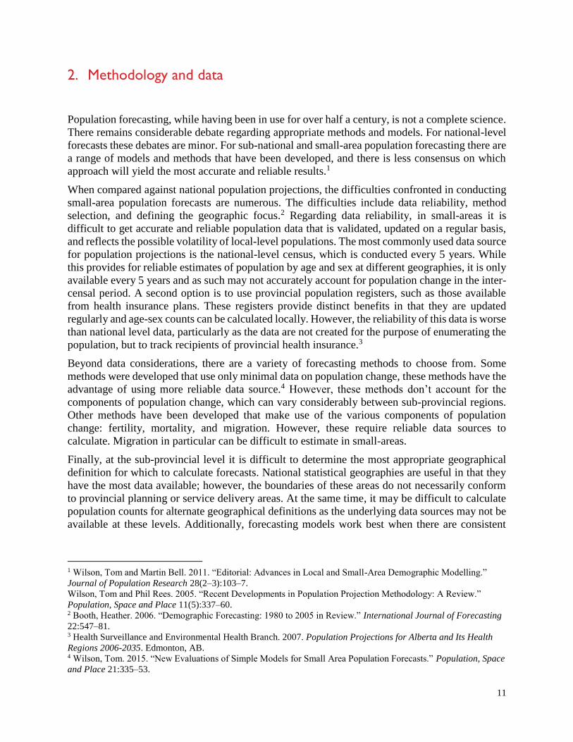
Table 1 summarises the range of scenarios used for constraining the population forecasts. These 7
provincial forecasts were developed by Statistics Canada, with variation in birth, death, and
migration rates.6 The purpose of having multiple projection scenarios is to reflect the uncertainty
associated with future direction of population change. The projection scenarios presented here are
constructed by combining several assumptions regarding the future evolution of each of the
components of population growth.
The five medium-growth scenarios (M1 through M5) were developed based on assumptions
reflecting different observed internal migration patterns. Each scenario puts forward a separate
assumption to reflect the volatility of this component. There is a high degree of volatility for
internal migration in New Brunswick, where inter-provincial and intra-provincial migration rates
5 Wilson, Tom. 2015. “New Evaluations of Simple Models for Small Area Population Forecasts.” Population, Space
and Place 21:335–53. 6 Statistics Canada. 2010. Population Projections for Canada, Provinces and Territories. 2009-2036. Ottawa, ON.
Retrieved (http://www.statcan.gc.ca/pub/91-520-x/91-520-x2010001-eng.htm).
13
are the largest single contributor to the variation in population change. Conversely, the steady
change in fertility and mortality rates has remained relatively consistent over the several past
decades.
The low-growth and high-growth scenarios bring together assumptions that are consistent with
either lower or higher population growth than in the medium-growth scenarios. For example,
assumptions that entail high fertility (Total Fertility Rate – TFR), low mortality, high immigration,
low emigration and high numbers of non-permanent residents are the foundation for the high-
growth scenario.
Essentially, the low-growth and high-growth scenarios are intended to provide a plausible and
sufficiently broad range of projected numbers to take account of the uncertainties inherent in any
population forecasting exercise. In the low-growth and high-growth scenarios, the interprovincial
migration assumption is the same as that used in the M1 medium-growth scenario, based on the
period 1991/1992 to 2010/2011.
Table 1: Summary of constrained scenarios assumptions, Statistics Canada 2014.
Scenario Fertility Life expectancy Immigration Migration trends
Low Low:
TFR=1.53
Low:
86.0 Male, 87.3 Female
Low: 5.0
(per 1,000) 1991 – 2011
M1 Medium:
TFR=1.67
Medium:
87.6 Male, 89.2 Female
Medium:
7.5 (per 1,000) 1991 – 2011
M2 Medium Medium Medium 1991 – 2000
M3 Medium Medium Medium 1999 – 2003
M4 Medium Medium Medium 2004 – 2008
M5 Medium Medium Medium 2009 – 2011
High High:
TFR=1.88
High:
89.9 Male, 91.1 Females
High:
9.0 (per 1,000) 1991 – 2011
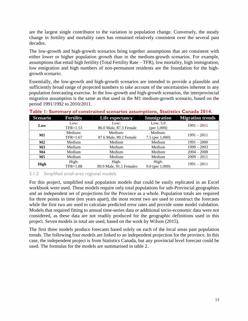
2.1.2 Simplified small-area regional models
For this project, simplified total population models that could be easily replicated in an Excel
workbook were used. These models require only total populations for sub-Provincial geographies
and an independent set of projections for the Province as a whole. Population totals are required
for three points in time (ten years apart), the most recent two are used to construct the forecasts
while the first two are used to calculate predicted error rates and provide some model validation.
Models that required fitting to annual time-series data or additional socio-economic data were not
considered, as these data are not readily produced for the geographic definitions used in this
project. Seven models in total are used, based on the work by Wilson (2015).
The first three models produce forecasts based solely on each of the local areas past population
trends. The following four models are linked to an independent projection for the province. In this
case, the independent project is from Statistics Canada, but any provincial level forecast could be
used. The formulas for the models are summarised in table 2.
14
Table 2: Models developed for simplified regional forecasts7.
Model Description Formula Models based on local area population trends
LIN Linear 𝑃𝑖(𝑡 + 1) = 𝑃𝑖(𝑡) + 𝐺𝑖 EXP Exponential 𝑃𝑖(𝑡 + 1) = 𝑃𝑖(𝑡)𝑒
𝑟𝑖
LIN_EXP Linear - Exponential If base period growth is positive:
𝑃𝑖(𝑡 + 1) = 𝑃𝑖(𝑡) + 𝐺𝑖 If base period growth is negative:
𝑃𝑖(𝑡 + 1) = 𝑃𝑖(𝑡)𝑒𝑟𝑖
Models linked to an independent Provincial forecast
CGD Constant growth rate
difference 𝑃𝑖(𝑡 + 1) = 𝑃𝑖(𝑡)𝑒
(𝑟𝑃𝑟𝑜𝑣(𝑡,𝑡+1)+𝐺𝑅𝐷𝑖)
CSP Constant share of population 𝑃𝑖(𝑡 + 1) = 𝑃𝑃𝑟𝑜𝑣(𝑡 + 1)𝑆𝐻𝐴𝑅𝐸𝑃𝑂𝑃𝑖(𝑡) CSG Constant share of growth 𝑃𝑖(𝑡 + 1) = 𝑃𝑖(𝑡)𝑆𝐻𝐴𝑅𝐸𝐺𝑅𝑂𝑊𝑇𝐻𝑖𝐺𝑃𝑟𝑜𝑣(𝑡, 𝑡 + 1) VSG Variable share of growth If base period growth is positive:
𝑃𝑖(𝑡 + 1) = 𝑃𝑖(𝑡) + 𝐺𝑖(𝑡, 𝑡 + 1) 𝑃𝑂𝑆𝐹𝐴𝐶𝑇𝑂𝑅𝑖(𝑡, 𝑡 + 1)
If base period growth is negative:
𝑃𝑖(𝑡 + 1) = 𝑃𝑖(𝑡) + 𝐺𝑖(𝑡, 𝑡 + 1) 𝑁𝐸𝐺𝐹𝐴𝐶𝑇𝑂𝑅𝑖(𝑡, 𝑡 + 1)
Notation:
Pi(t) jump-off year population of small area i
Pi(t+1) projected population of small area i at time t+1
Gi annual average population growth over the base period
ri annual average population growth rate of small area i over the base period
GRDi base period growth rate difference
SHAREPOPi(t) share of Provincial population in small area i at jump-off year t
SHAREGROWTHi small area’s share of Provincial population growth in the base period
GProv forecast Provincial population growth
POSFACTORi(t,t+1) plus-minus adjustment factor for positive growth
NEGFACTORi(t,t+1) plus-minus adjustment factor for negative growth
2.1.3 Small-area cohort-component models
Population forecasts via a cohort component model divides the forces of population change into
six parts: fertility, mortality, in-migration, out-migration, immigration, and emigration. Each of
component is modeled as a rate, which is then applied to a base (or “jump”) population over a
given period via a Leslie matrix. Successive applications of the rates over the given interval and
model parameters produce the population forecasts.
The parameters of the model may be changed to obtain different scenarios. For the current project,
four levels are considered for each component: baseline (B), low (L), median (M), and high (H).
The baseline level corresponds to the rates derived directly from the data, where each geographic
area maintains the rate calculated from administrative data sources. In contrast, the low, median,
and high scenarios, respectively, use the first quartile, median, and third quartile, of the rates by
age and sex.
The current project uses 20 age categories and 2 sexes. The first age category includes individuals
from birth to just under one year of age (<1 year); the second pertains to individuals aged one year
7 Wilson, Tom. 2015. “New Evaluations of Simple Models for Small Area Population Forecasts.” Population, Space
and Place 21:335–53.

15
to less than 5 (1 to <5); the subsequent age categories are all of five years in length, except for the
last, which is open-ended.
Table 3: Primary projection scenarios for cohort-component modelling.
Scenario Fertility Mortality In-
migration
Out-
migration
Immigration Emigration
1 Base Base Base Base Base Base
2 Base Base Base Base Base High
3 Base Base Base Base Base Low
4 Base Base Base Base Base Median
5 Base Base Base Base High Base
6 Base Base Base Base High Low
7 Base Base Base Base Low Base
8 Base Base Base Base Median Base
9 Base Base Base High Base Base
10 Base Base Base Low Base Base
11 Base Base Base Median Base Base
12 Base Base High Base Base Base
13 Base Base Low Base Base Base
14 Base Base Median Base Base Base
15 Base High Base Base Base Base
16 Base Low Base Base Base Base
17 Base Median Base Base Base Base
18 High Base Base Base Base Base
19 High High High High High High
20 High Low Base Base High Low
21 Low Base Base Base Base Base
22 Low Low Base Base Low High
23 Low Low Low Low Low Low
24 Median Base Base Base Base Base
25 Median Median Base Base Median Median
26 Median Median Median Median Median Median
For each geographic definition, 26 scenarios have been developed, covering the years 2006
through 2056.
2.2 Selected data
The data required for the two forecasting techniques come from different sources. First, for the
simplified small-area forecasts, only total population counts are used. Second, small-area cohort-
component models require estimates of population, births, deaths, inter-provincial migration, intra-
provincial migration, immigration, and emigration. These data come from a variety of sources and
require different degrees of data management for use in population forecasting.
16
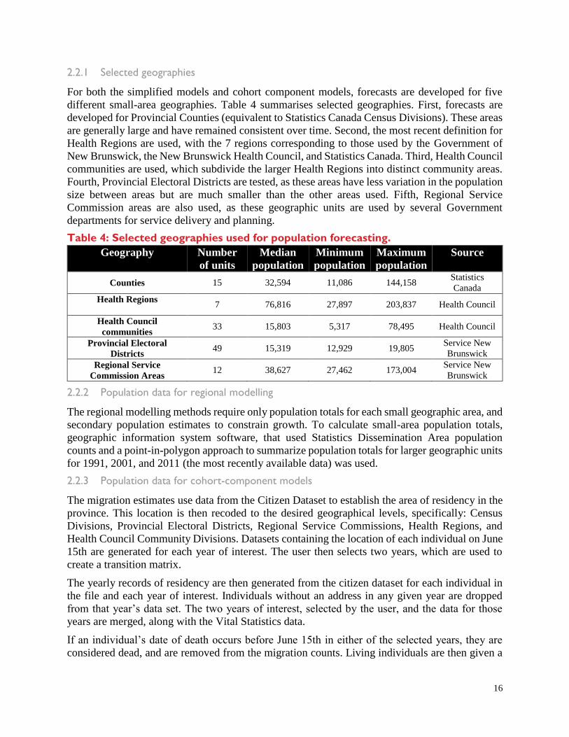
2.2.1 Selected geographies
For both the simplified models and cohort component models, forecasts are developed for five
different small-area geographies. Table 4 summarises selected geographies. First, forecasts are
developed for Provincial Counties (equivalent to Statistics Canada Census Divisions). These areas
are generally large and have remained consistent over time. Second, the most recent definition for
Health Regions are used, with the 7 regions corresponding to those used by the Government of
New Brunswick, the New Brunswick Health Council, and Statistics Canada. Third, Health Council
communities are used, which subdivide the larger Health Regions into distinct community areas.
Fourth, Provincial Electoral Districts are tested, as these areas have less variation in the population
size between areas but are much smaller than the other areas used. Fifth, Regional Service
Commission areas are also used, as these geographic units are used by several Government
departments for service delivery and planning.
Table 4: Selected geographies used for population forecasting.
Geography Number
of units
Median
population
Minimum
population
Maximum
population
Source
Counties 15 32,594 11,086 144,158 Statistics
Canada
Health Regions
7 76,816 27,897 203,837 Health Council
Health Council
communities 33 15,803 5,317 78,495 Health Council
Provincial Electoral
Districts 49 15,319 12,929 19,805
Service New
Brunswick
Regional Service
Commission Areas 12 38,627 27,462 173,004
Service New
Brunswick
2.2.2 Population data for regional modelling
The regional modelling methods require only population totals for each small geographic area, and
secondary population estimates to constrain growth. To calculate small-area population totals,
geographic information system software, that used Statistics Dissemination Area population
counts and a point-in-polygon approach to summarize population totals for larger geographic units
for 1991, 2001, and 2011 (the most recently available data) was used.
2.2.3 Population data for cohort-component models
The migration estimates use data from the Citizen Dataset to establish the area of residency in the
province. This location is then recoded to the desired geographical levels, specifically: Census
Divisions, Provincial Electoral Districts, Regional Service Commissions, Health Regions, and
Health Council Community Divisions. Datasets containing the location of each individual on June
15th are generated for each year of interest. The user then selects two years, which are used to
create a transition matrix.
The yearly records of residency are then generated from the citizen dataset for each individual in
the file and each year of interest. Individuals without an address in any given year are dropped
from that year’s data set. The two years of interest, selected by the user, and the data for those
years are merged, along with the Vital Statistics data.
If an individual’s date of death occurs before June 15th in either of the selected years, they are
considered dead, and are removed from the migration counts. Living individuals are then given a

17
weight for their contributions towards each age category. For example, if an individual is 48 in the
first year and 53 in the second year, they would be given a weight of respectively 0.4 and 0.6 for
the 45 – 50, and 50 – 55 year age categories. The weights are then summed up by region, which
creates a transition matrix containing migration estimates, with a row and a column for each
geographic region.
Estimated migration rates are then computed by dividing the number of migrants in an area by the
population of potential migrants (and multiplying the quotient by one thousand). For the rates of
(internal) in-migration, the number of incoming migrants is divided by the sum of incoming
migrants and of non-migrants in each other region. Similarly, for the rates of (internal) out-
migration, the number of out-going migrants is divided by the sum of out-going migrants,
emigrants, and non-movers from the region. Emigration rates are calculated by dividing the
number of emigrants by the same denominator used for the out-migration rates.
Unlike the others, the total number of potential immigrants is unknown, so the rate of immigration
has been estimated as a ratio immigrants and the sum of out-going migrants, emigrants, and non-
movers from the region. The rationale behind this supposition is that geographic areas will attract
migrants in proportion to their population in the first year.
18
3. Simplified small-area forecasts
The population in New Brunswick is experiencing consistent demographic shifts in fertility and
mortality. Concurrently, there are large fluctuations in migration and immigration. The declines in
fertility are like those experienced across developed nations, where the general fertility rate is
declining and age-specific rates are shifting to older age groups. The declines in mortality, while
smaller in New Brunswick than in other provinces, are also like those seen in other jurisdictions.
However, the patterns of migration in New Brunswick are distinct and have a high degree of
temporal and geographic variation. As such, it is important that any population forecasting
undertaken at the small-area level recognise the potential for shifts in migration rates and provide
a range of scenarios.
As described in the methods section, two approaches of population forecasting were developed,
each presenting multiple scenarios of population change. This section of the report focusses on
simplified methods of calculating small-area population forecasts, where only the population totals
for each period are used. The subsequent section presents a cohort-component model where
forecasts make use of the components of population change and present results by age and sex.
Recent research has shown that the use of simplified regional growth models can provide robust
estimates of population change for smaller geographic units. These models are constructed using
only regional population counts over multiple time periods, combined with external population
forecasts. A multi-stage approach is taken, where models are first validated against past data points
and historic population forecasts, and the appropriate models are selected. Following this, models
are constructed using current population counts, with small-area growth-rates constrained to the
external Provincial population forecasts.
3.1 Population change, by county
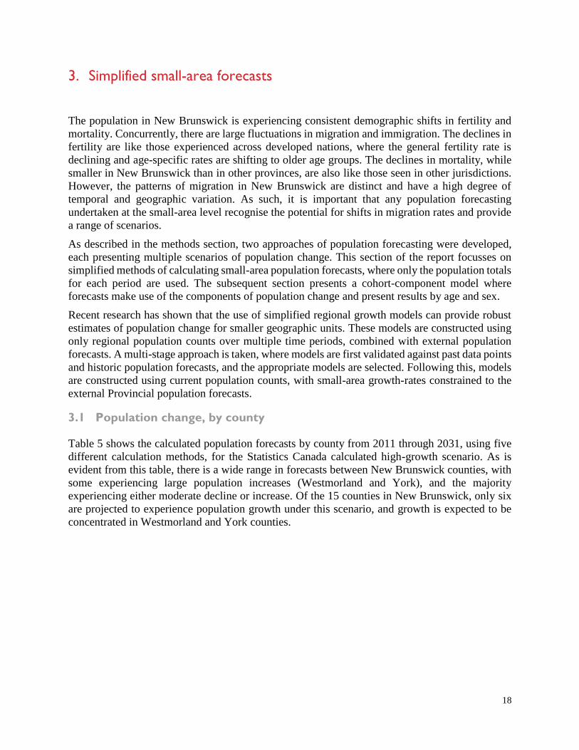
Table 5 shows the calculated population forecasts by county from 2011 through 2031, using five
different calculation methods, for the Statistics Canada calculated high-growth scenario. As is
evident from this table, there is a wide range in forecasts between New Brunswick counties, with
some experiencing large population increases (Westmorland and York), and the majority
experiencing either moderate decline or increase. Of the 15 counties in New Brunswick, only six
are projected to experience population growth under this scenario, and growth is expected to be
concentrated in Westmorland and York counties.
19
Table 5. Population change (2011-2031) and annual growth rates by constrained
model, high growth scenario1, by county.
Total population change by model, 2011 - 2031
Increase
per year
Growth
rate per
year County LIN EXP LIN_EXP CGD VSG Saint John 2,948 1,109 2,705 1,475 877 217 0.0029
Charlotte -2,080 -2,634 -2,213 -2,670 -1,299 -82 -0.0030
Sunbury 2,227 1,692 2,067 1,653 1,319 137 0.0052
Queens -1,728 -1,823 -1,632 -1,834 -711 -78 -0.0068
Kings 9,566 8,928 9,136 8,852 6,672 546 0.0082
Albert 5,952 6,324 7,046 6,318 4,462 327 0.0120
Westmorland 37,568 43,067 36,582 43,197 28,974 2,028 0.0152
Kent -1,627 -2,344 -1,758 -2,389 -1,348 -55 -0.0018
Northumberland -5,713 -6,461 -5,599 -6,519 -2,750 -246 -0.0050
York 19,276 20,223 18,644 20,190 14,368 1,061 0.0116
Carleton -799 -1,464 -942 -1,506 -1,051 -17 -0.0006
Victoria -2,822 -3,048 -2,915 -3,069 -1,224 -125 -0.0061
Madawaska -4,912 -5,258 -4,679 -5,293 -2,088 -219 -0.0063
Restigouche -7,568 -7,237 -6,715 -7,251 -2,556 -354 -0.0103
Gloucester -11,516 -12,305 -10,958 -12,385 -4,876 -514 -0.0064
* Total population of New Brunswick is constrained to a high growth scenario, which uses mean migration
rates from 1981 through 2008
Table 5 shows models calculated via several different regional methods. As outlined in the
methodology section, each of these methods has different advantages depending the rate of change,
whether the change is positive or negative, and the size of the base population.
Table 6 shows the estimated errors for the available models, as calculated at the county level. From
analysis of the selected constrained models at the county level, the models with the lowest Median
Average Percent Error between 2001 and 2011 were the LIN, EXP, and VSG models. Of these,
the EXP and VSG models had the lowest overall errors and thus are presented as the primary
options in this report.
Table 6. Estimated errors for constrained projection models, 2001-2011, census
divisions.
Median
absolute %
error
Median %
error
Mean
absolute %
error
Mean %
error % Negative
% with
<10%
absolute %
error
LIN 5.44 4.89 6.22 3.15 0.00 86.67
EXP 5.83 4.62 6.14 3.08 0.00 93.33
LIN_EXP 6.03 4.83 6.21 3.14 0.00 86.67
CGD 5.93 4.71 6.23 3.11 0.00 86.67
CSP 7.58 6.08 7.95 3.94 0.00 60.00
CSG 7.77 3.25 9.82 1.94 0.00 66.67
VSG 2.94 1.19 4.66 3.39 0.00 80.00
20
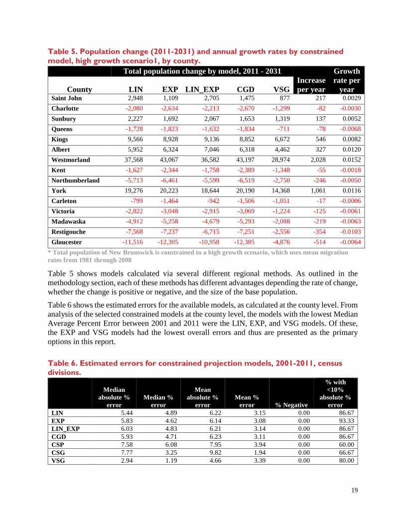
Table 7 shows the range of population forecasts between the different constrained growth scenarios
using the variable share of growth method. (The specifics for the growth scenarios is outlined in
Table 1.) The difference between the low and high forecasts reflects the range of possible
provincial scenarios, with the variation in the medium growth scenarios reflecting changes in inter-
provincial migration rates. Given the high degree of variation in inter-provincial migration, these
differences are not surprising.
For the M1 scenario, inter-provincial migration rates are based on the average between 1991 and
2011, thus minimising the period effects that are seen in the other medium-growth scenarios. The
M2 scenario uses inter-provincial migration rates from 1991 through 2000, which in New
Brunswick was a period near the mean. Inter-provincial migration in 1991 – 2003 was not as high
as in more recent periods. The M4 scenario uses inter-provincial migration rates from between
2004 and 2008, which for New Brunswick coincided with an exceptionally high rate of provincial
out-migration. As such, the M4 scenario has the largest overall population decline over the 20-
year period, even more than for the low-growth scenario. In contrast, the M5 scenario uses inter-
provincial migration rates from 2009 – 2011, which coincided with the period after the 2008
recession, where there were low rates of out-migration and the only recent period of net in-
migration.
Table 7. Total forecast population change (2011-2031), variable share of growth
method, by growth scenario, by county.
County Low M1 M2 M3 M4 M5 High Saint John -1,235 -282 -145 -290 -1,272 450 877
Charlotte -2,036 -1,706 -1,658 -1,708 -2,047 -1,451 -1,299
Sunbury 32 612 696 607 9 1,058 1,319
Queens -1,352 -1,067 -1,026 -1,070 -1,361 -845 -711
Kings 1,612 3,892 4,221 3,873 1,524 5,648 6,672
Albert 1,459 2,812 3,007 2,801 1,407 3,854 4,462
Westmorland 10,401 18,766 19,974 18,697 10,076 25,214 28,974
Kent -1,878 -1,639 -1,605 -1,641 -1,886 -1,457 -1,348
Northumberland -4,855 -3,915 -3,779 -3,923 -4,885 -3,187 -2,750
York 4,605 9,003 9,638 8,967 4,434 12,392 14,368
Carleton -1,249 -1,159 -1,146 -1,160 -1,252 -1,091 -1,051
Victoria -2,269 -1,804 -1,737 -1,808 -2,284 -1,442 -1,224
Madawaska -3,908 -3,099 -2,981 -3,105 -3,935 -2,468 -2,088
Restigouche -5,313 -4,097 -3,919 -4,107 -5,352 -3,138 -2,556
Gloucester -9,144 -7,246 -6,970 -7,261 -9,205 -5,766 -4,876
New Brunswick -15,130 9,070 12,570 8,870 -16,030 27,770 38,770
Based on these models and under a range of scenarios, only six of the 15 Counties in New
Brunswick are forecast to have any population growth over the next 20 years. Two counties –
Westmorland (Moncton & Dieppe) and York (Fredericton) – will concentrate most of this growth.
While these figures are only based on prior data and from population totals, it suggests that without
some external changes (economic, social, policy, environmental), most New Brunswick counties
will continue to see population decline over the long term.
Map 3 shows the distribution of this forecasted population change across New Brunswick at the
county level. As is evident, even in the high-growth scenario, the only projected population growth
is in the south of the province and concentrated in Moncton, Fredericton, and the outskirts of Saint
John.

21
Map 3: High growth scenario by county, 2011 – 2031.
Map 4 shows the forecasted population change across New Brunswick under a low-growth
scenario. As is evident, under this scenario the only projected population growth is in the south of
the province and concentrated in Moncton, Fredericton, and the outskirts of Saint John. Most
growth would occur in the area surrounding Moncton. This scenario is a good comparison to the
high-growth scenario as it uses the same migration assumptions, where migration is averaged
across 1991 through 2011. The difference between low and high growth scenarios is only with
fertility, mortality, and international immigration.

22
Map 4: Low growth scenario by county, 2011 – 2031.
Map 5 furthers these scenarios by presenting a forecast for medium rates of fertility, mortality, and
international immigration. As with the previous maps, migration rates were calculated as the
average between 1991 and 2011. It is only under this scenario that higher growth appears in the
Fredericton region and outside of Saint John, likely driven by growth in Quispamsis.

23
Map 5: Medium (M1) growth scenario by county, 2011 – 2031.
3.1.1 Population forecasts for selected counties
Under the various growth scenarios there are a range of potential outcomes for each county in New
Brunswick. While some of these counties (Westmorland & York) will see population growth under
all scenarios, most counties have the potential for population decline in the long-term, even under
high-growth.
The population forecasts for Saint John County (Figure 1) exhibit a range of outcomes depending
on the growth scenario selected. In the low-growth scenario, there is a continued decrease in the
population of Saint John County over time. However, for this county the lowest growth occurs in
the medium growth M4 scenario, which corresponds with high levels of provincial out-migration.
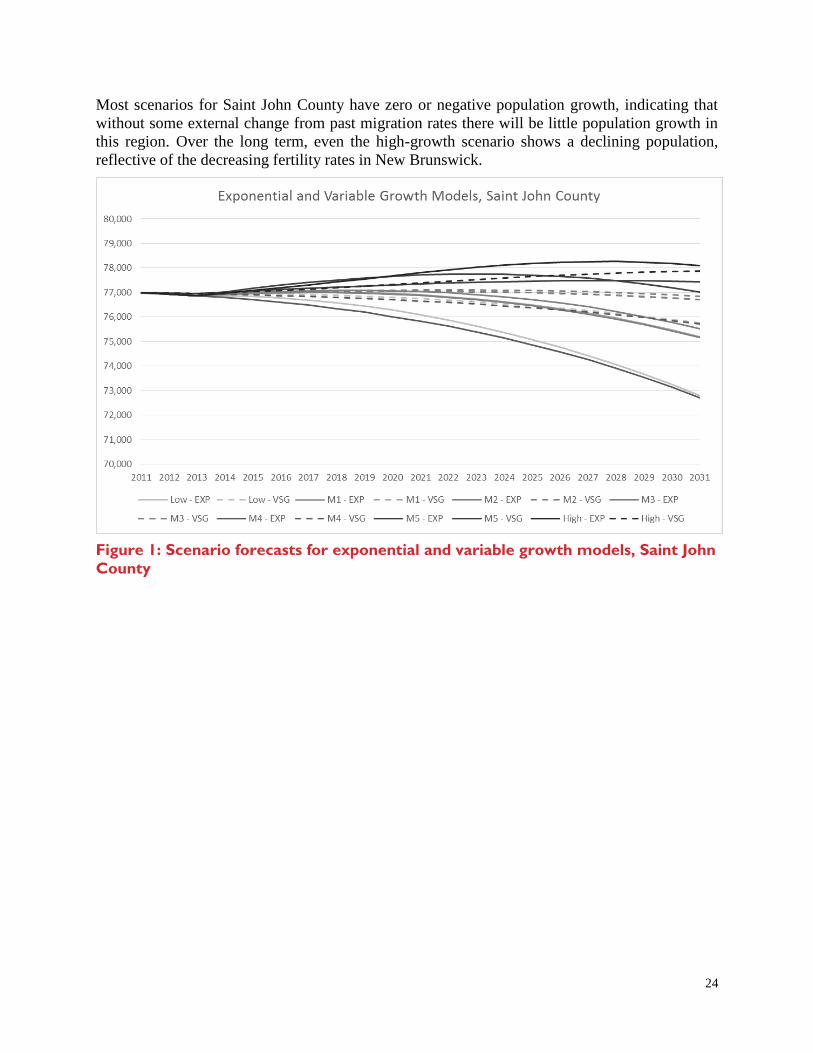
24
Most scenarios for Saint John County have zero or negative population growth, indicating that
without some external change from past migration rates there will be little population growth in
this region. Over the long term, even the high-growth scenario shows a declining population,
reflective of the decreasing fertility rates in New Brunswick.
Figure 1: Scenario forecasts for exponential and variable growth models, Saint John
County
25
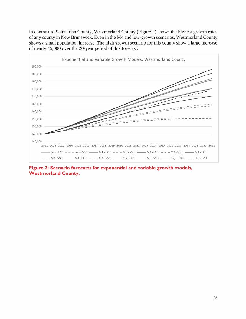
In contrast to Saint John County, Westmorland County (Figure 2) shows the highest growth rates
of any county in New Brunswick. Even in the M4 and low-growth scenarios, Westmorland County
shows a small population increase. The high growth scenario for this county show a large increase
of nearly 45,000 over the 20-year period of this forecast.
Figure 2: Scenario forecasts for exponential and variable growth models,
Westmorland County.

26
As with the results for Westmorland County, York County (Figure 3) shows steady growth
between 2011 and 2031. As with the other results presented here, the lowest growth is for the
low-growth and M4 scenarios, still resulting in a small increase of several thousand people. For
this county, the exponential (EXP) models show higher growth than does the variable share of
growth (VSG) model. This is difference is due to the nature of the models, where the EXP
method exaggerates sub-regions with higher growth rates and the EXP tends to mediate the
effect of rate differences between counties.
Figure 3: Scenario forecasts for exponential and variable growth models, York
County.
In terms of numbers, the highest projected growth for York County results in an increase of
approximately 20,000 people. The factors that would contribute to this increase are higher
immigration rates, lower out-migration rates, and consistent fertility rates. However, as the largest
drivers of the change are migration, changes to these rates will be driven largely by external factors
(economic growth, policy changes) than by family decisions (fertility).

27
More typical of New Brunswick counties, the results for Restigouche County (Figure 4) show a
continued decline in the population. Interestingly, the high growth scenarios are not those that
correspond to a slower rate of population decline. These results confirm that the major drivers of
population decline in this county are from out-migration, and that under conditions of high growth,
out-migration may increase in peripheral regions.
Figure 4: Scenario forecasts for exponential and variable growth models,
Restigouche County.

28
The results for Gloucester County (Figure 5) are similar to those for Restigouche, where if
historic trends continue, a decline in the population can be expected. From these models, the
population levels are less important than the direction of change, where it is evident that
irrespective of what scenario is selected there is predicted to be a decline in population.
Figure 5: Scenario forecasts for exponential and variable growth models,
Gloucester County.
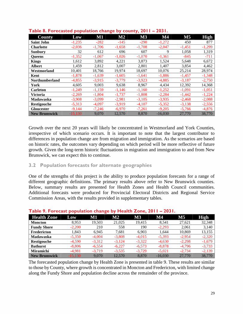
Table 8 shows the range of potential outcomes under the various forecast scenarios for each county
in New Brunswick between 2011 and 2031. For most counties, irrespective of which scenario is
assumed, there is no change between either population decline or population growth. The only
exception is for Saint John County, where the low-growth scenario shows a small decline, while
the high-growth scenario shows a small increase – less than 1,000 persons over 20 years.
For other counties, the growth rates (positive or negative) are very small over the 20-year period.
Increases or decreases of 1,000 to 2,000 persons over this time-period are not considerable. The
largest declines could be seen in Northumberland, Restigouche, and Gloucester and the largest
increases in Westmorland and York.
29
Table 8. Forecasted population change by county, 2011 – 2031.
County Low M1 M2 M3 M4 M5 High Saint John -1,235 -282 -145 -290 -1,272 450 877
Charlotte -2,036 -1,706 -1,658 -1,708 -2,047 -1,451 -1,299
Sunbury 32 612 696 607 9 1,058 1,319
Queens -1,352 -1,067 -1,026 -1,070 -1,361 -845 -711
Kings 1,612 3,892 4,221 3,873 1,524 5,648 6,672
Albert 1,459 2,812 3,007 2,801 1,407 3,854 4,462
Westmorland 10,401 18,766 19,974 18,697 10,076 25,214 28,974
Kent -1,878 -1,639 -1,605 -1,641 -1,886 -1,457 -1,348
Northumberland -4,855 -3,915 -3,779 -3,923 -4,885 -3,187 -2,750
York 4,605 9,003 9,638 8,967 4,434 12,392 14,368
Carleton -1,249 -1,159 -1,146 -1,160 -1,252 -1,091 -1,051
Victoria -2,269 -1,804 -1,737 -1,808 -2,284 -1,442 -1,224
Madawaska -3,908 -3,099 -2,981 -3,105 -3,935 -2,468 -2,088
Restigouche -5,313 -4,097 -3,919 -4,107 -5,352 -3,138 -2,556
Gloucester -9,144 -7,246 -6,970 -7,261 -9,205 -5,766 -4,876
New Brunswick -15,130 9,070 12,570 8,870 -16,030 27,770 38,770
Growth over the next 20 years will likely be concentrated in Westmorland and York Counties,
irrespective of which scenario occurs. It is important to note that the largest contributor to
differences in population change are from migration and immigration. As the scenarios are based
on historic rates, the outcomes vary depending on which period will be more reflective of future
growth. Given the long-term historic fluctuations in migration and immigration to and from New
Brunswick, we can expect this to continue.
3.2 Population forecasts for alternate geographies
One of the strengths of this project is the ability to produce population forecasts for a range of
different geographic definitions. The primary results above refer to New Brunswick counties.
Below, summary results are presented for Health Zones and Health Council communities.
Additional forecasts were produced for Provincial Electoral Districts and Regional Service
Commission Areas, with the results provided in supplementary tables.
Table 9. Forecast population change by Health Zone, 2011 – 2031.
Health Zone Low M1 M2 M3 M4 M5 High Moncton 8,953 19,503 21,025 19,415 8,541 27,621 32,348
Fundy Shore -2,200 210 558 190 -2,293 2,061 3,140
Fredericton 1,843 6,945 7,681 6,903 1,644 10,869 13,155
Madawaska -5,350 -4,004 -3,808 -4,015 -5,393 -2,954 -2,320
Restigouche -4,590 -3,312 -3,124 -3,322 -4,630 -2,298 -1,679
Bathurst -8,806 -6,554 -6,227 -6,573 -8,878 -4,796 -3,733
Miramichi -4,981 -3,719 -3,535 -3,729 -5,021 -2,734 -2,139
New Brunswick -15,130 9,070 12,570 8,870 -16,030 27,770 38,770
The forecasted population change by Health Zone is presented in table 9. These results are similar
to those by County, where growth is concentrated in Moncton and Fredericton, with limited change
along the Fundy Shore and population decline across the remainder of the province.
30
Table 10. Forecast population change by Health Council community, 2011 – 2031.
Community Low M1 M2 M3 M4 M5 High Kedgwick -828 -654 -629 -656 -834 -518 -435
Campbellton -1,971 -1,552 -1,491 -1,556 -1,984 -1,224 -1,025
Dalhousie -2,706 -2,108 -2,021 -2,113 -2,725 -1,636 -1,348
Bathurst -3,667 -2,967 -2,866 -2,973 -3,689 -2,425 -2,098
Caraquet -2,398 -1,878 -1,802 -1,882 -2,415 -1,468 -1,219
Shippegan -2,286 -1,800 -1,730 -1,804 -2,301 -1,420 -1,189
Tracadie-Sheila -728 -666 -657 -667 -730 -619 -592
Neguac -1,077 -862 -831 -864 -1,084 -694 -593
Miramichi -4,128 -3,330 -3,214 -3,336 -4,153 -2,710 -2,336
Bouctouche -1,781 -1,474 -1,430 -1,477 -1,791 -1,238 -1,096
Salisbury -107 -9 5 -10 -110 66 110
Shediac 562 1,437 1,563 1,430 528 2,111 2,504
Sackville -201 -76 -59 -77 -205 19 74
Riverview 2,028 3,470 3,679 3,458 1,972 4,582 5,229
Moncton 4,663 8,465 9,014 8,434 4,514 11,395 13,102
Dieppe 5,730 9,039 9,517 9,011 5,600 11,590 13,076
Hillsborough -637 -511 -493 -512 -641 -414 -355
Sussex -916 -893 -890 -893 -916 -876 -866
Minto -1,247 -991 -954 -994 -1,255 -792 -671
Saint John -1,064 -75 67 -83 -1,102 685 1,127
Grand Bay-Westfield -343 -305 -299 -305 -344 -276 -259
Quispamsis 2,538 4,556 4,848 4,539 2,459 6,111 7,017
St. George -1,122 -919 -890 -921 -1,128 -762 -668
St. Stephen -948 -834 -818 -835 -952 -747 -695
Oromocto -281 -48 -15 -50 -290 131 235
Fredericton 5,328 9,005 9,536 8,975 5,185 11,839 13,490
New Maryland 872 1,806 1,941 1,798 835 2,525 2,944
Nackawic -738 -643 -630 -644 -742 -571 -527
Douglas -124 132 169 130 -134 329 443
Florenceville-Bristol -1,283 -1,194 -1,182 -1,195 -1,285 -1,128 -1,088
Perth-Andover -1,507 -1,188 -1,141 -1,190 -1,517 -937 -785
Grand Falls -1,924 -1,549 -1,495 -1,552 -1,936 -1,258 -1,082
Edmunston -2,840 -2,310 -2,234 -2,315 -2,857 -1,900 -1,653
New Brunswick -15,130 9,070 12,570 8,870 -16,030 27,770 38,770
The forecasted population change by Health Council community (Table 10) are more variable than
for larger geographic areas and thus need to be interpreted with more caution. However, these
geographically disaggregated results provide some important insight into where growth and
decline may occur over the medium term. The most notable difference is that Shediac has emerged
as a potential area for growth over the next 20 years, with positive population change irrespective
of the scenario. Other areas that could see moderate growth are Sackville, Saint John, Oromocto,
and Douglas.
Map 6 shows the forecasted population change for Health Council communities under the High
Growth scenario. This scenario uses migration rates averaged over the 1991-2011 period, thus
minimising the variation in internal and external migration patterns that are exhibited at the
provincial level.
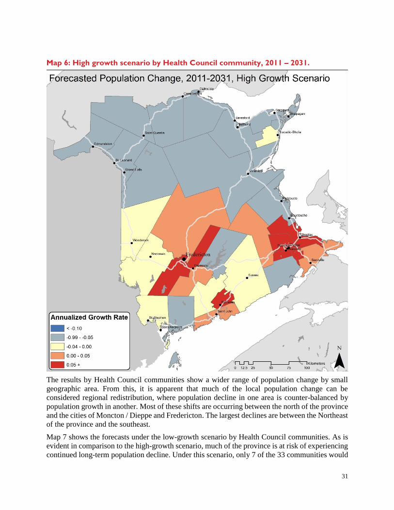
31
Map 6: High growth scenario by Health Council community, 2011 – 2031.
The results by Health Council communities show a wider range of population change by small
geographic area. From this, it is apparent that much of the local population change can be
considered regional redistribution, where population decline in one area is counter-balanced by
population growth in another. Most of these shifts are occurring between the north of the province
and the cities of Moncton / Dieppe and Fredericton. The largest declines are between the Northeast
of the province and the southeast.
Map 7 shows the forecasts under the low-growth scenario by Health Council communities. As is
evident in comparison to the high-growth scenario, much of the province is at risk of experiencing
continued long-term population decline. Under this scenario, only 7 of the 33 communities would

32
experience a population increase, with the majority of the province experiencing population
decline. This scenario is a useful comparison in contrast to the high-growth as it uses the same
migration assumptions, where migration is averaged across the 1991 through 2011 period. Thus,
the only elements that change between these two are fertility, mortality, and immigration.
Map 7: Low growth scenario by Health Council community, 2011 – 2031.
The scenario presented in Map 8 shows a medium-growth scenario, where migration is also
averaged over the 1991-2011 period. Thus, this map is similar to the high and low growth scenarios
except for fertility, mortality, and international immigration. Under these conditions, 9
communities would experience some growth over the 20-year period, although all growth would
remain in the areas surrounding Fredericton, Moncton, and Saint John.

33
Map 8: Medium (M1) growth scenario by Health Council community, 2011 – 2031.
The final scenario presented here is the medium-growth, M5 scenario, which considers medium
growth where migration patterns are similar to those experienced in the 2009-2011 period. This is
significant for New Brunswick, as this period was a shortened period of return-migration following
the 2008 financial crisis and down-turn in the Alberta economy. This “bust” period where there
was a slowdown in resource extraction resulted in a slowing of inter-provincial out-migration and
an increase in inter-provincial in-migration. As such, it is illustrative of the potential that exists if
total out-migration is reduced and in-migration is moderately increased.

34
Map 9: Medium (M5) growth scenario by Health Council community, 2011 – 2031.
3.3 Summary of simplified small-area models
Simplified small-area models provide a quick and reliable means to estimate population change
across New Brunswick. The primary advantage of this method is that it only relies on only
population totals and secondary population estimates. Despite this, these models are shown to be
flexible in that they provide a range of outcomes when combined with external growth scenarios.
The total population of New Brunswick is forecasted to grow only moderately in the next decades.
Based on historic trends, growth has been slow and prone to a high degree of local-level
fluctuation. Population increases are concentrated in only a few regions. At higher levels of

35
geography, only the areas surrounding Fredericton and Moncton show potential for growth. A
narrower focus suggests that areas such as Shediac, Sackville, St. John, Oromocto, and Douglas
represent opportunities for population growth. However, the majority of the province is likely
facing a continued gradual decline. The range of scenarios presented does little to change predicted
declines.

36
4. Small-area cohort component forecasts
In the second phase of this project, a cohort-component model was developed that accounts for
directional migration between New Brunswick regions and for independently varying, small-area
differences in fertility and mortality rates. The scenarios generated via these models use person-
level administrative data from the New Brunswick Citizen Database, Vital Statistics, and growth
rates derived from regional observations. The advantages of this approach include the flexibility
in modelling, where new scenarios can be generated quickly, the use of provincial administrative
data that correspond to the population on an annual basis, and the use of rates derived from the
range of possibilities within the province.
Building on the findings above, the components of population change will be examined in more
detail through a series of cohort-component models. First, a set of base models are presented that
reflect the range of possible growth outcomes as observed from the administrative micro-data.
Second, these results are constrained to the external population change scenarios from Statistics
Canada. This allows for small-area variation in growth rates, while limiting population change to
the overall predicted values for New Brunswick. Third, inter-provincial migration and immigration
are isolated and the potential effect that these rates would have on overall population change is
examined. Fourth, the forecasted shift in the age-sex distribution is examined for the primary
forecasts.
Results are presented here at the county and the Health Council community levels. Other
geographic aggregations were also calculated.
4.1 Population change by county
The initial cohort-component models developed examine how forecasted population change would
differ depending on the input rates. For these scenarios, four primary models are presented: low,
baseline, median, and high (Table 11). In the low model, all component rates are set to the lowest
regional rate. For the baseline model, all small-area rates are set to their calculated values from the
administrative data. In the median model, the rates are calculated as the median rate observed
across all areas. In the high model, the highest rate from each area is used. Together, these four
scenarios provide a set of forecasts that fall within the range of observed values.

37
Table 11. Unconstrained population change, by scenario, by county, 2006 - 2036.
County Low Baseline Median High Saint John 3,165 4,851 7,118 11,761
Charlotte 826 1,800 2,202 3,814
Sunbury 4,015 16,633 5,629 7,542
Queens -1,045 764 -619 -119
Kings 5,657 21,475 9,330 13,628
Albert 1,584 8,577 3,043 4,752
Westmorland 5,775 12,425 12,412 20,197
Kent -454 581 897 2,481
Northumberland 601 -703 3,004 5,811
York 6,127 14,132 10,892 16,493
Carleton 1,777 4,936 3,266 5,015
Victoria 1,066 2,520 2,172 3,482
Madawaska -10 -1,798 1,478 3,224
Restigouche -569 -1,403 928 2,691
Gloucester -1,385 -8,169 1,867 5,656
The forecasted population change across the four scenarios (Table 11) is predicted to be moderate
for most counties. In the low-growth scenario, Queens, Kent, Madawaska, Restigouche, and
Gloucester Counties are predicted to have population declines. Under the high rate scenario, only
Queens County will have some population decline. In all scenarios, Sunbury, Kings, Westmorland,
York, and Carleton Counties will have population growth, with the largest growth occurring in
Kings, Westmorland, and York Counties.
Table 12. Unconstrained rates of change, by scenario, by county, 2006 - 2036.
County Low Baseline Median High Saint John 0.04 0.06 0.09 0.16
Charlotte 0.03 0.07 0.08 0.14
Sunbury 0.18 0.73 0.25 0.33
Queens -0.09 0.06 -0.05 -0.01
Kings 0.09 0.33 0.14 0.21
Albert 0.06 0.31 0.11 0.17
Westmorland 0.05 0.10 0.10 0.16
Kent -0.01 0.02 0.03 0.08
Northumberland 0.01 -0.01 0.06 0.11
York 0.07 0.16 0.13 0.19
Carleton 0.07 0.18 0.12 0.19
Victoria 0.05 0.12 0.10 0.17
Madawaska 0.00 -0.05 0.04 0.09
Restigouche -0.02 -0.04 0.03 0.08
Gloucester -0.02 -0.10 0.02 0.07
When the rates of change (Table 12) are considered, rather than just the predicted values of
population change, a different picture of population dynamics is presented. The largest growth
rates appear in Sunbury and Kings Counties. Most counties have only moderate growth rates
between 0.03 and 0.10 with little variation between scenarios. Where there is greater variation
between scenarios, it is suggestive of a high degree of variability in the underlying data,
particularly for migration rates. These rates tend to fluctuate over time, and the lowest observed

38
rate may be considerably different from the highest. In contrast, fertility and mortality are relatively
stable over time and therefore observed differences are likely not large.
Table 13. Constrained population change, by scenario, by county, 2006 - 2036.
County Low M1 M2 M3 M4 M5 High Saint John -1,810 1,653 2,124 1,653 -1,780 4,167 5,897
Charlotte -970 254 420 254 -965 1,146 1,760
Sunbury 2,638 3,839 4,002 3,839 2,652 4,704 5,304
Queens -1,879 -1,410 -1,347 -1,410 -1,877 -1,071 -835
Kings 1,247 4,421 4,850 4,421 1,277 6,715 8,294
Albert -273 1,017 1,193 1,017 -264 1,955 2,599
Westmorland -2,789 3,117 3,918 3,117 -2,732 7,394 10,335
Kent -2,666 -1,305 -1,124 -1,305 -2,655 -322 357
Northumberland -2,871 -609 -302 -609 -2,852 1,030 2,151
York 434 4,522 5,077 4,522 469 7,483 9,524
Carleton 14 1,284 1,453 1,284 26 2,205 2,836
Victoria -318 651 784 651 -309 1,356 1,842
Madawaska -2,454 -942 -741 -942 -2,436 150 896
Restigouche -2,999 -1,502 -1,299 -1,502 -2,988 -413 333
Gloucester -7,115 -3,690 -3,220 -3,690 -7,081 -1,207 502
Table 13 shows the forecasted scenarios of population change, constrained to the seven scenarios
generated by Statistics Canada. Underlying these scenarios are the baseline rates observed from
the New Brunswick microdata (the baseline scenario in Table 11). In comparison to the
unconstrained rates, the population changes are moderated between growth scenarios.
Unsurprisingly, the lowest growth occurs in the low-growth scenario, where the only counties with
a positive population increase are Sunbury, Kings, York, and Carleton Counties. In contrast, the
only county with a negative growth in the high scenario is Queens County.
When considered as rates of change (Table 14), these differences become much smaller. For
instance, in Queens County, the rates of change vary between -0.09 (M5 scenario) and -0.15 (low
growth). In Sunbury County, growth rates vary between 0.11 (M5) scenario and 0.23 (high
growth). These difference show that the changes in rates between scenarios is independent between
counties, where for some counties the lowest growth scenario doesn’t always indicate the lowest
predicted growth rate. Likewise, for some counties the highest growth scenario doesn’t necessarily
translate into the highest growth rate.

39
Table 14. Constrained rates of change, by scenario, by county, 2006 - 2036.
County Low M1 M2 M3 M4 M5 High Saint John -0.02 0.02 0.03 0.02 -0.02 0.05 0.08
Charlotte -0.03 0.01 0.02 0.01 -0.03 0.04 0.06
Sunbury 0.11 0.16 0.17 0.16 0.11 0.20 0.23
Queens -0.15 -0.12 -0.11 -0.12 -0.15 -0.09 -0.07
Kings 0.02 0.06 0.07 0.06 0.02 0.10 0.12
Albert -0.01 0.04 0.04 0.04 -0.01 0.07 0.09
Westmorland -0.02 0.02 0.03 0.02 -0.02 0.06 0.08
Kent -0.08 -0.04 -0.03 -0.04 -0.08 -0.01 0.01
Northumberland -0.05 -0.01 -0.01 -0.01 -0.05 0.02 0.04
York 0.00 0.05 0.06 0.05 0.01 0.08 0.11
Carleton 0.00 0.05 0.05 0.05 0.00 0.08 0.10
Victoria -0.01 0.03 0.04 0.03 -0.01 0.06 0.09
Madawaska -0.07 -0.03 -0.02 -0.03 -0.07 0.00 0.03
Restigouche -0.08 -0.04 -0.04 -0.04 -0.08 -0.01 0.01
Gloucester -0.09 -0.04 -0.04 -0.04 -0.09 -0.01 0.01
What the above tables illustrate most is the high degree of variability in the predicted population
change across geographic areas. Depending on what base rates are used, growth can vary between
negative and positive values, and result in a large decrease in the population or a large increase.
That said, it is important recognise that any population change that does occur will likely be driven
largely by internal and inter-provincial migration rates.
4.2 Potential effects of inter-provincial migration
To examine the effects of inter-provincial migration on population change, table 15 shows the
differences if only out-migration rates varied. For these scenarios, the remaining components of
population change (fertility, mortality, emigration, immigration, and in-migration) were held
constant, and only rates of out-migration varied. In the low out-migration scenario, the lowest
observed out-migration rate was used for all geographic areas. In the high migration scenario, the
highest observed out-migration rate was used. As such, the count reflects the net population
difference between these two.
The first column in table 15 shows the forecasted population in 2036 under the low out-migration
scenario. The second column shows the forecasted population under the high out-migration
scenario. The last two columns show the difference between the baseline population in 2006 and
the forecasted population under each scenario.
In the low out-migration scenario, the only region that would experience a small decline is Queens
County, with all others experiencing an increase. The majority of the increase would go to
Sunbury, Kings, Westmorland, and York Counties. Under a high out-migration scenario, Sunbury,
Kings, and York Counties would see a population increase while most of the counties would see a
decrease.
It is important to note that these differences are from changes to only out-migration rates. As such,
it is the effect of only people leaving an area that is measured, with the assumption that all
individuals leaving an area will be leaving the province. The conclusions that can be drawn from
this relate to the degree to which overall population change is effected by shifts in out-migration

40
to other provinces. Even in large regions such as Westmorland, which consistently shows the
highest overall population growth rate, the effect of out-migration is pronounced. Within a
balanced model, the in-migration and immigration rates counteract out-migration to result in
population growth. The skewed out-migration model shows the degree to which this component
of population change contributes to overall growth rates in small geographic areas.
Table 15. Potential effect of out-migration, by county, 2006-2036.
County Forecasted
population,
Low Scenario
Forecasted
population,
High Scenario
Low scenario,
baseline
difference
High scenario,
baseline
difference Saint John 83,535 73,474 5,943 -4,118
Charlotte 32,595 28,657 4,782 844
Sunbury 37,934 32,950 14,367 9,383
Queens 12,106 10,636 -48 -1,518
Kings 86,269 75,792 18,246 7,769
Albert 33,241 29,230 4,708 697
Westmorland 145,382 128,165 13,533 -3,684
Kent 34,270 30,305 1,879 -2,086
Northumberland 57,819 50,903 5,559 -1,357
York 105,266 92,457 16,307 3,498
Carleton 35,145 30,658 7,408 2,921
Victoria 24,978 21,916 3,433 371
Madawaska 37,012 32,711 1,637 -2,664
Restigouche 38,486 33,997 2,680 -1,809
Gloucester 82,410 73,215 408 -8,787
* In this scenario, out-migration rates are set at the lowest or highest rate with all other rates set to baseline.
Table 16 extends this analysis to examine the effect that in-migration would have on population
change. As is clear from these numbers, the difference between the low and high in-migration
scenarios is minimal. In this table, the first two columns show the forecasted population in 2036
under a baseline scenario where in-migration rates are either set to the lowest or highest observed.
For instance, Kings County has a forecasted population change of 20,972 between 2006 and 2036
in the high in-migration scenario. In the low in-migration scenario this difference from baseline is
only 19,807, or a difference of 1,165 persons.

41
Table 16. Potential effect of in-migration, by county, 2006-2036.
County Forecasted
Population,
Low Scenario
Forecasted
Population,
High Scenario
Low Scenario,
Baseline
Difference
High Scenario,
Baseline
Difference Saint John 80,701 81,751 3,109 4,159
Charlotte 28,404 28,767 591 954
Sunbury 39,191 39,756 15,624 16,189
Queens 12,368 12,533 214 379
Kings 87,830 88,995 19,807 20,972
Albert 36,085 36,559 7,552 8,026
Westmorland 142,545 144,360 10,696 12,511
Kent 31,701 32,085 -690 -306
Northumberland 49,568 50,189 -2,692 -2,071
York 101,027 102,352 12,068 13,393
Carleton 31,415 31,845 3,678 4,108
Victoria 23,120 23,422 1,575 1,877
Madawaska 32,148 32,534 -3,227 -2,841
Restigouche 32,972 33,375 -2,834 -2,431
Gloucester 71,011 71,826 -10,991 -10,176
* In this scenario, in-migration rates are set at the lowest or highest rate with all other rates set to baseline.
Comparing the results of the in-migration and out-migration scenarios, it is suggestive that out-
migration plays a much greater role in the population dynamics of New Brunswick than in-
migration. As well, the difference between low and high out-migration rates is large; when the
highest out-migration rates are applied to regions that traditionally have lower rates, there are
marked differences in the forecasted populations.
Moving from migration, the following section examines the potential shifts in the age distribution
in New Brunswick.
4.3 Changing age distribution
There are predicted to be large shifts in the underlying age distribution of New Brunswick. Over
the last decades, dependency ratios have changed markedly, with the proportion of the population
over the age of 65 increasing at a greater pace than in other Canadian provinces. Conversely, the
youth dependency ratio has decreased, with a smaller proportion of the population under the age
of 15.
By constructing detailed cohort-component models using administrative micro-data, it is possible
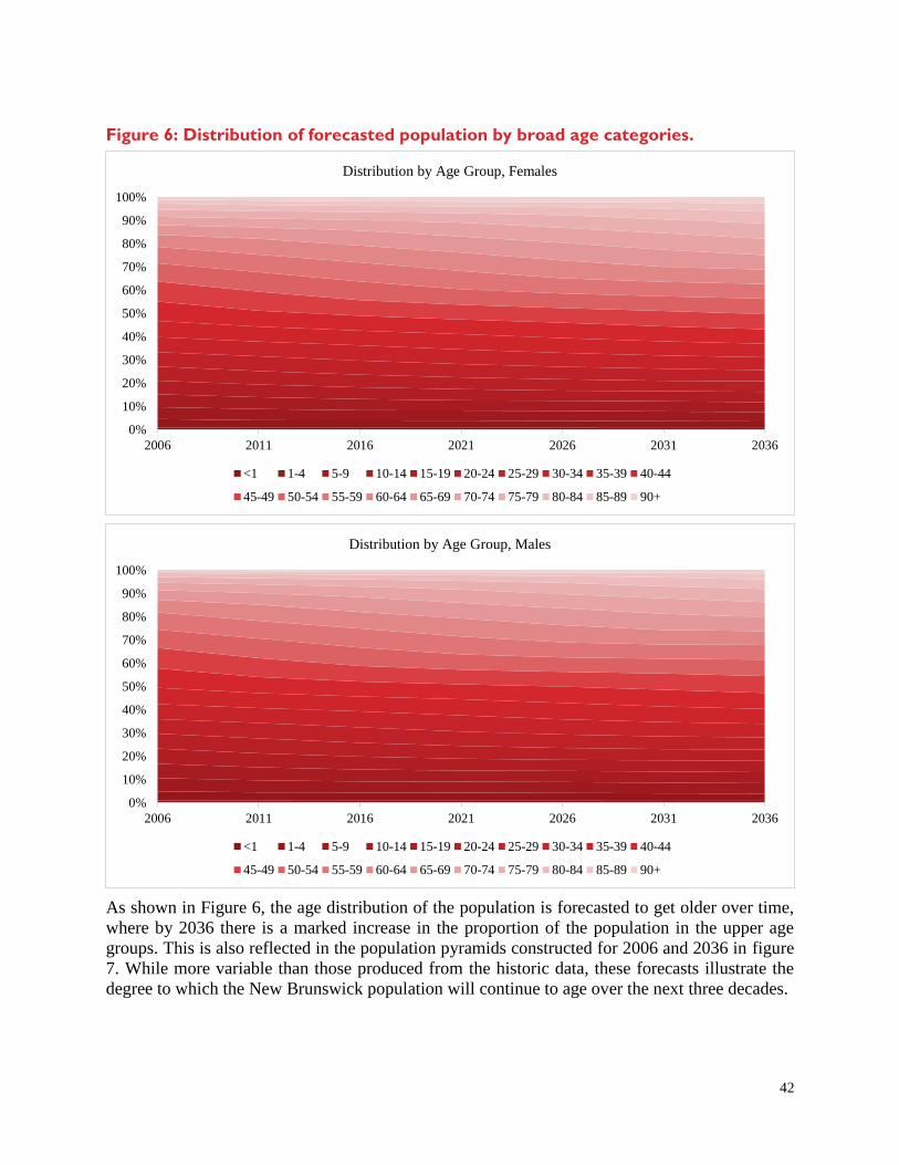
to examine the potential changes in age distribution over time. Figure 6 shows the distribution of
the population by broad age categories under the baseline scenario. In 2006, females over the age
of 65 make up 16% of the total female population. By 2036, females over the age of 65 are
predicted to be 31% of the female population. Males 65 and over make up 12.5% of the population
in 2006, which is predicted to increase to 26% by 2036. For youth under the age of 15, it is
predicted that they will decrease from 15% for females (17% for males) to 12% for females and
13% for males.
42
Figure 6: Distribution of forecasted population by broad age categories.
As shown in Figure 6, the age distribution of the population is forecasted to get older over time,
where by 2036 there is a marked increase in the proportion of the population in the upper age
groups. This is also reflected in the population pyramids constructed for 2006 and 2036 in figure
7. While more variable than those produced from the historic data, these forecasts illustrate the
degree to which the New Brunswick population will continue to age over the next three decades.
0%
10%
20%
30%
40%
50%
60%
70%
80%
90%
100%
2006 2011 2016 2021 2026 2031 2036
Distribution by Age Group, Females
<1 1-4 5-9 10-14 15-19 20-24 25-29 30-34 35-39 40-44
45-49 50-54 55-59 60-64 65-69 70-74 75-79 80-84 85-89 90+
0%
10%
20%
30%
40%
50%
60%
70%
80%
90%
100%
2006 2011 2016 2021 2026 2031 2036
Distribution by Age Group, Males
<1 1-4 5-9 10-14 15-19 20-24 25-29 30-34 35-39 40-44
45-49 50-54 55-59 60-64 65-69 70-74 75-79 80-84 85-89 90+

43
Figure 7: Population pyramids for 2006 and 2036, baseline scenario.
0-4
5-9
10-14
15-19
20-24
25-29
30-34
35-39
40-44
45-49
50-54
55-59
60-64
65-69
70-74
75-79
80-84
85-89
90+
Population Distribution by Age Group, 2006
Females Males
0-4
5-9
10-14
15-19
20-24
25-29
30-34
35-39
40-44
45-49
50-54
55-59
60-64
65-69
70-74
75-79
80-84
85-89
90+
Population Distribution by Age Group, 2036
Females Males
44
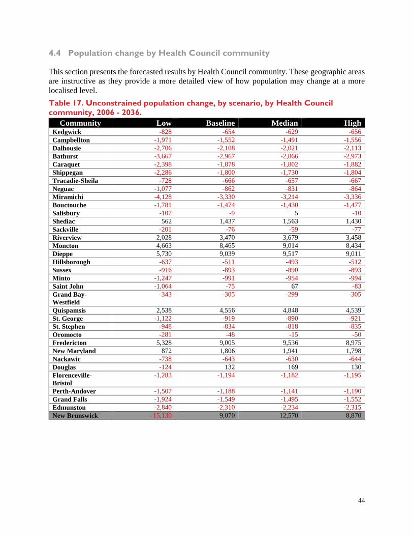
4.4 Population change by Health Council community
This section presents the forecasted results by Health Council community. These geographic areas
are instructive as they provide a more detailed view of how population may change at a more
localised level.
Table 17. Unconstrained population change, by scenario, by Health Council
community, 2006 - 2036.
Community Low Baseline Median High Kedgwick -828 -654 -629 -656
Campbellton -1,971 -1,552 -1,491 -1,556
Dalhousie -2,706 -2,108 -2,021 -2,113
Bathurst -3,667 -2,967 -2,866 -2,973
Caraquet -2,398 -1,878 -1,802 -1,882
Shippegan -2,286 -1,800 -1,730 -1,804
Tracadie-Sheila -728 -666 -657 -667
Neguac -1,077 -862 -831 -864
Miramichi -4,128 -3,330 -3,214 -3,336
Bouctouche -1,781 -1,474 -1,430 -1,477
Salisbury -107 -9 5 -10
Shediac 562 1,437 1,563 1,430
Sackville -201 -76 -59 -77
Riverview 2,028 3,470 3,679 3,458
Moncton 4,663 8,465 9,014 8,434
Dieppe 5,730 9,039 9,517 9,011
Hillsborough -637 -511 -493 -512
Sussex -916 -893 -890 -893
Minto -1,247 -991 -954 -994
Saint John -1,064 -75 67 -83
Grand Bay-
Westfield
-343 -305 -299 -305
Quispamsis 2,538 4,556 4,848 4,539
St. George -1,122 -919 -890 -921
St. Stephen -948 -834 -818 -835
Oromocto -281 -48 -15 -50
Fredericton 5,328 9,005 9,536 8,975
New Maryland 872 1,806 1,941 1,798
Nackawic -738 -643 -630 -644
Douglas -124 132 169 130
Florenceville-
Bristol
-1,283 -1,194 -1,182 -1,195
Perth-Andover -1,507 -1,188 -1,141 -1,190
Grand Falls -1,924 -1,549 -1,495 -1,552
Edmunston -2,840 -2,310 -2,234 -2,315
New Brunswick -15,130 9,070 12,570 8,870

45
Table 18. Constrained rates of change, by scenario, by Health Council community,
2006 - 2036.
Community Low M1 M2 M3 M4 M5 High Kedgwick -828 -654 -629 -656 -834 -518 -435
Campbellton -1,971 -1,552 -1,491 -1,556 -1,984 -1,224 -1,025
Dalhousie -2,706 -2,108 -2,021 -2,113 -2,725 -1,636 -1,348
Bathurst -3,667 -2,967 -2,866 -2,973 -3,689 -2,425 -2,098
Caraquet -2,398 -1,878 -1,802 -1,882 -2,415 -1,468 -1,219
Shippegan -2,286 -1,800 -1,730 -1,804 -2,301 -1,420 -1,189
Tracadie-Sheila -728 -666 -657 -667 -730 -619 -592
Neguac -1,077 -862 -831 -864 -1,084 -694 -593
Miramichi -4,128 -3,330 -3,214 -3,336 -4,153 -2,710 -2,336
Bouctouche -1,781 -1,474 -1,430 -1,477 -1,791 -1,238 -1,096
Salisbury -107 -9 5 -10 -110 66 110
Shediac 562 1,437 1,563 1,430 528 2,111 2,504
Sackville -201 -76 -59 -77 -205 19 74
Riverview 2,028 3,470 3,679 3,458 1,972 4,582 5,229
Moncton 4,663 8,465 9,014 8,434 4,514 11,395 13,102
Dieppe 5,730 9,039 9,517 9,011 5,600 11,590 13,076
Hillsborough -637 -511 -493 -512 -641 -414 -355
Sussex -916 -893 -890 -893 -916 -876 -866
Minto -1,247 -991 -954 -994 -1,255 -792 -671
Saint John -1,064 -75 67 -83 -1,102 685 1,127
Grand Bay-
Westfield
-343 -305 -299 -305 -344 -276 -259
Quispamsis 2,538 4,556 4,848 4,539 2,459 6,111 7,017
St. George -1,122 -919 -890 -921 -1,128 -762 -668
St. Stephen -948 -834 -818 -835 -952 -747 -695
Oromocto -281 -48 -15 -50 -290 131 235
Fredericton 5,328 9,005 9,536 8,975 5,185 11,839 13,490
New Maryland 872 1,806 1,941 1,798 835 2,525 2,944
Nackawic -738 -643 -630 -644 -742 -571 -527
Douglas -124 132 169 130 -134 329 443
Florenceville-
Bristol
-1,283 -1,194 -1,182 -1,195 -1,285 -1,128 -1,088
Perth-Andover -1,507 -1,188 -1,141 -1,190 -1,517 -937 -785
Grand Falls -1,924 -1,549 -1,495 -1,552 -1,936 -1,258 -1,082
Edmunston -2,840 -2,310 -2,234 -2,315 -2,857 -1,900 -1,653
New Brunswick -15,130 9,070 12,570 8,870 -16,030 27,770 38,770

46
Discussion
This report has presented a detailed analysis of population change in New Brunswick through an
elaboration of small-area population forecasts using multiple methods and data sources. Population
change in New Brunswick is a continued source of discussion in the Province.
The results of this report show that changes to rates of population growth are largely dependent on
migration patterns. When out-migration has been low, there has been a small overall population
increase. However, when out-migration is high there has been an overall population decline. While
in-migration and immigration are counteracting population decline to some extent, the degree to
which out-migration is effecting population dynamics in small-areas is large. As such, relevant
policies for population growth will need to address concrete reasons for out-migration.
In this report we have identified several current population issues for New Brunswick:
Forecasted population growth is only predicted in around the the cities of Moncton, Fredericton
and Saint John;
There is a continued aging of the population, with very high old-age dependency ratios; and.
Inter-provincial out-migration is driving population change in the Province.
Opportunities to reverse the current trends of low growth, net inter-Provincial migration losses,
and traditionally low immigration exist in the areas of:
1. Address continued out-migration by:
a. Providing high-quality and low-cost educational opportunities for youth.
b. Invest in cultural capital targeted towards youth and young families.
c. Generate employment opportunities within New Brunswick, even if not within hometowns.
d. Ensure level of government services matches that available in other Provinces.
2. Focus on new immigration opportunities:
a. Providing services, training, and cultural support for new immigrants & families.
b. Support private immigration sponsorship and family reunification schemes.