SLAC-PUB-120 July 1965

GROUP THEORY AND TJ33 HYDROGEN ATOM*

M. Bander and C. Itzykson+

Stanford Linear Accelerator Center S%anford Utiversiiy, Stanford, Caiifornia

ABSTRACT

The internal O(4) symmetry group of the non-relativistic

hydrogen atom is discussed and used to relate the various approaches

to the bound state problems. A more general group 0(1,4) of

transformations is shown to connect the various levels, which

appear as basis vectors for a continuous set of unitary repre-

sentations of this non compact group.

(Submitted to Journal of Mathematical Physics)

* Work supported by the U. S. Atcmic Energy Commission.

t On leave of absence from Service de Physique Theorique CEN

Saclay, B.P. No. 2, Gif sur Yvette (S. et O.), PRANCE.

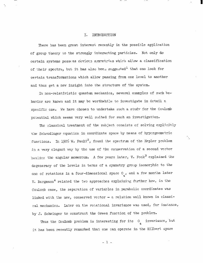
I. IIYTRODUCTION

There has been great interest recently in the possible application

of group theory to the strongly interacting particles. Not only do

certain systems poss<.ss obvious Symmetries which allow a classification

of their spectra, but it has als; beeu suggested' that one look for

certain transformations which allow passing from one level to another

and thus get a new insight into the structure of the system.

In non-relativistic quantum mechanics, several examples of such be-

havior are known and it may be worthwhile to investigate in detail a

specific one. We have chosen to undertake such a study for the Coulomb

potential which seems very well suited for such an investigation.

The classical treatment of the subject consists of solving explicitly

the Schrodinger equation in coordinate space by means of hypergeometric

functions. III 1926 W. Pauli;?, found the spectrum of the Kepler problem

in a very elegant way by the use of the conservation of a second vector

besides the angular momentum. A few years later, V. Fock3 explained the

degeneracy of the levels in terms of a symmetry group isomorphic to the

one of rotations in a four-dimensional space 0 4’

and a few months later

V. Bargmann4 related the two approaches explaining further how, in the

Coulomb case, the separation of variables in parabolic coordinates was

linked with the new, conserved vector - a relation well known in classi-

cal mechanics. Later on the rotational invariance was used, for instance,

by J. Schwinger to construct the Green function of the problem.

Thus the Coulollib problem is interesting for its O4 invariance, but

it has been recently remarked that one can operate in the Hilbert space

- l-

I

of bound states with a still larger group, isomorphic to the de-Sitter

group, O(L4L in such a way that one thus gets an irreducible infinite

dimensional unitary representation of this non-compact group.

Our aim has thus been twofold, We first review the symmetry group

- o&the syste,:, descrLing succ1.-xtl; the ---?tf:ods d.isccssed above. We

note some further relations which were implicit in the works quoted

above. Actually, following a remark of Alliluev: we shall even gener-

alize the problem to an arbitrary number of dimensions. The larger

group, W,% is then introduced in an heuristic way, The new ter-

minology suggested for this kind of superstructure is "Physical Trans-

formation Group." We shall write the explicit realization of this group

as a set of unitary operations in the Hilbert space of bound states and

prove irreducibility using the infinitesimal generators0 Finally, it

is suggested that the type of considerations used can be generalized to

obtain special types of unitary representations for non-compact groups.

This paper is mainly concerned with the problem of bound states. We

hope to consider in the future the case of scattering states.

Several recent lectures given at Stanford by Professor Y. Ne'eman

were the inspiration for this work. It is a pleasure to thank him for

his stimulation. It is clear that many of the results were known to

him and certainly to many other physicists. We apologize in advance

for giving only a very sketchy bibliography.

-2-

- I

II. THE SYMMETRY GROUP

A. The Infinitesimal Method2

We want to solve the Schrodinger equation for the Coulomb potential

with n the Laplacian

a2 A=---

3X2 1

a2 a2 +-+-

a, 2

7 ax2

r= dFFY$-,

2 3

P is the reduced mass and, in the case of an hydrogen-like atom,

k = Ze2 . Let Pi 35 a

=miy then due to the invariance of Eq. (1)

under spatial rotation the angular momentum

L ij = x.p. - x.p. 1J J1 $ = EkijLij

- (2)

is conserved, and it is possible to separate the equation using polar

coordinates. However, it is known that in the Kepler problem, the

following three vector

is also a constant of the motion, e is the velocity, 2 the angular

momentum, and ; the position vector, ; = (xl, x2, x3). Pauli simply

used the correspondence principle and investigated the commutation rela-

tions of the Hermitian part of the previous vector, i.e.,

--

The commutation relations of E , M' and the Hamiltonian H are

[H,Li] = 0

[H,M~I = 0

[Lj’L$ = ifiEjk&L& (4)

and

L 'M=M'L=O (ti - k2) = ; H(L2 + fi2) . (5)

--. I

Relations (4) suggest the consideration of a subspace belonging to the

eigenvalue E(E < 0) of the Hamiltonian as L and M commute with it.

In this subspace it is meaningful to introduce the operator

f;ii = i- SE Mi

L+z and L-G Then, as a result, 2 - 2 build up two commuting sets of

operators, each one satisfying the commutation relations of ordinary L+i2 angular momentum; hence 2 c ) = Ti2j,(j, + 1) and (9)' = fi2j2(j2 + 1) -

But according to Eq. (5)’ L l i = c l L = 0 so that

--

. l.e., J =

1 j2 . It is not clear at this point whether j = j = j2 1

has to be limited to integer values or can also take half-integer values.

Assuming for a moment that 2j can t&e any integer value, we derive

-4 -

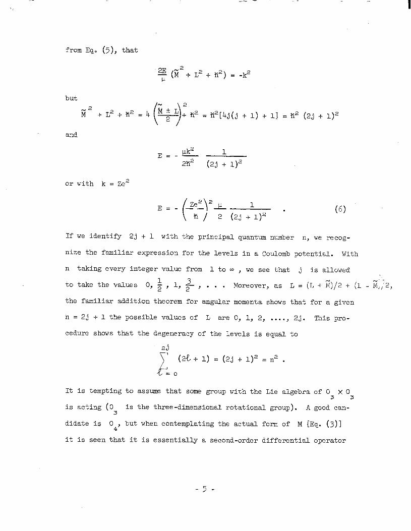
from Eq. (5)’ that

$ (G2 + L2 + h2) = -k2

but

ii2 +L2+;K2=4 = %i2[4j(j + 1) + 11 = h2 (2j + 1)2

and

E=-!ic 1 2$ (2j + 1)2

or with k = Ze"

I; 1

2 (2j + 1)2 l

(6)

If we identify 2j + 1 with the principal quantum number n, we recog-

nize the familiar expression for the levels in a Coulomb potential. With

n taking every integer value from 1 to M , we see that j is allowed

3 to take the values 0, $ , 1, 2 , . . , ----

Moreover, as L = (L + $/' + (L - M,;2,

the familiar addition theorem for angular momenta shows that for a given

n = 2j + 1 the possible values of L are 0, 1, 2, . . . . . 2j. Ihis pro-

cedure shows that the degeneracy of the levels is equal to

2j

F

(2&+ 1) = (2j + 1)' = n2 .

=o

It is tempting to assume that some group with the Lie algebra of 0 x 0 3 3

is acting (0 3 is the three-dimensional rotational group). A good can-

didate is 0 4’

but when contemplating the actual form of M [Eq. (3)]

it is seen that it is essentially a second-order differential operator

-5 -

in coordinate space. However, since the main part is linear in x,

there might be some suspicion that it would be interesting to look in

p-space for we know that properly parametrized infinitesimal generators

are linear differential operators. This explains the second approach to

the symmetry due to Fock.

B. The Global Method'

We rn$<e a Fourier transformation and write the equation in momentum

space. The 1 F term gives rise to a convolution integral and we find

k Q (P> = 2~2K s

d3qQh) .

I i - $1'

In fact, it will be of some interest to follow the remark of Allilue$

that the method can be generalized to any number of dimensions greater

than or equal to 2. The dimension will be denoted by f. We have

1 1 -=- r fiw

f-1

.-+ -+ -1qor

where a, n is the area of the unit hypersphere in an n-dimensional space

&v5 (J =--

n I$ 0

For dimension f, Eq. (7) generalized to

(7’ >

Let us remark that, in the case of bound states, E is negative. We

-6-

-. I

introduce the quantity

Pg = - 2mE >o,

and the equation now reads

1< r 9 ( J (P2 f Pg) 0 (P) = - -- r aTryJ

dfq Q’(q)

I + f-l

C-P I

(8)

(9)

In this form the equation seem; to e--hi..lit nothing more than the

usual f-dimensional rotational invariance. We now perform a change of

variable o First, we replace $ by Z/P,, then imbed the f-dimensional

space in an f + 1 dimensional one and perform a stereographic projec-

tion on the unit sphere (Fig. 1).

Let ': be the point on the unit sphere corresponding to $ and let z

denote the unit vector from the origin to the north pole of the sphere;

we have

;:= P2 - PZ +

2p0 n+ P2 + P; P2 + $

s .

An immediate calculation shows that

I

df+ku = 2&(u2 - l)df+lu = (2Po)f

dfp

(Pg + P2)f

I 1; - ;I’ = (P2 + pZ)(q2 f PZ) + I

+ 2 u-v I

(2Po)2

if v' +

corresponds to q. Let us also change the wave function by

defining

; (u) = -L p; + p2 2

4- PO ( ) f-t1

Q(P) 2p0

(10)

(11)

(12)

-7-

Inserting these values in Eq. (9) we get

I

vk a(u) = -

2P035 (13)

The great interest of Eq. (13) is to show that the problem is

rotationally invarian". in iin f+l-dimensional space, which in the case

of f=3 implies an 0 4

symmetry grxp. Lefcre solving Eq, (13) it

is interesting to compare the normalization of g and Q,wehave

s I&>I 2dS2u = s PZ + P2

2P; I ( )I Q p 2dfp

We can now use the virial theorem which eta%?

E s I~b)(‘dfp = - .f $- (@cd i2dfp to obtain the result that [for a solution of Eq. (13)

(14)

Hence the mapping: 0(p), belonging to the eigenvalue E,-;(u)

satisfying Eq. (13) as given by conditions (10) and (12) preserves the

scalar products. This mapping can be extended on one side to the Hilbert

space of L2 functions on the sphere - call it;: Y f+l, on the other to

the Hilbert space of linear combinations of e?genfunctions (and their

limits) corresponding to the discrete spectrum of the Hamiltonian. As

the functions corresponding to different eigenvalues of the Hamiltonian

are orthogonal and as the same property holds on the sphere for solutions I

of Eq, (13) corresponding to different eigenvalues of p, , the extended

mapping.obtained in that way is one-to-one and isometric that is unitary.

-8-

-- - .-

Note that it cannot be given through a geometric transformation of the

type (10) which clearly depends on po8 . We now solve Eq. (13), using

the following remark. In the f + l-dimensional space, the kernel

1;; - :, is essentially the Green function of the Laplace operator.

z f- 1

tiore precisely,

*ft 1 1 L: -f f-1=

I’: - VI

- (f - l)'"f+ff+l(Ti - ;, . (15)

Moreover, the spherical harmonics defined on the sphere form a complete

system of functions in, % $1' They are lsbelled by an integer A taking

the values 0,1,2,... and an index cx whose meaning will be specified in

a moment, such that if YA,o: is the spherical harmonic

is an homogeneous polynomial of degree h in G constrained by the

condition

af++&(;) = 0. (16)

The index a allows us to classify the set of solutions of Eq. (16)

properly orthonormalized. An arbitrary homogeneous polynomial in f+l

variables of degree A depends on constants.

Equation (16) gives homogeneous conditions; hence the

-9-

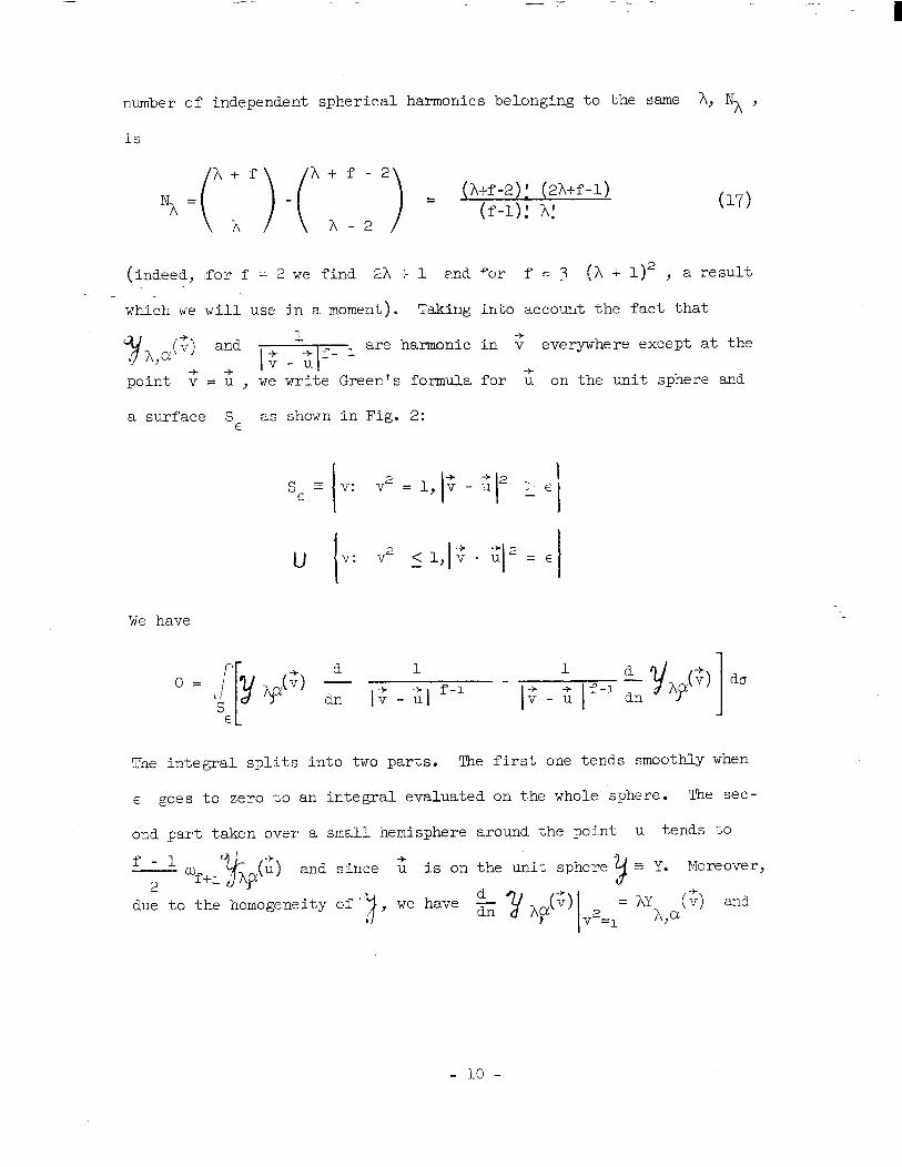
number of independent spherical harmonics belonging to the same A, NA ,

is

07)

(indeed, for f = 2 we find 2A :- 1 and

which we will use in a moment). Taking -f

&A ) V and );1 are harmonic

point T,L; , we write Green's formula

a surface S E as shown in Fig. 2:

SE = I

v: v2 = 1, f - I

We have

o= ,/ S E

%r f - _? (A + 1)2 , a result

into account the fact that

in ; everywhere except at the

for z on the unit sphere and

1

1; - "1 f-1

The integral splits into two parts. The first one tends smoothly when

e goes to zero to an integral evaluated on the whole sphere. The sec-

ond part taken over a small hemisphere around the point u tends to

f-l - c.o~+~$&$;) and since t is on the unit sphere y - Y. Moreover, 2

due to the homogeneity d

, we have -d-n- v2=1

- 10 -

-- -. I

on the sphere v2 = 1 (with u2 = 1)

d 1

Helice

f-l 1 = -- 2 I

+ f-21 z-u I

v 2 =u2q V2

2 =u =I.

f--1 f-l d- i-2 f-l

o= - ~f+ry~cr(a + 2 I s 1; _ ;Lf- l$j-@ - -y - A [ 1

Using again the formula for the area of the sphere, we get

Y&) = (f - l+ 2A)

f+1 I? / b-z-

Ye, &I O-8)

Equation (13) is now to be compared with Eq. (1.8). Obviously, due to

the completeness of spherical harmonics, we have thus found all the

possible levels given by

pk -f-1+2A -- PO5

2

thus

P: CL k2 EC-Vi- -

2P 2 y12' (19)

If we go back on earth and set f = 3, then f - 2' + 2A = A + 1 and

we again get formula (6) with A now identified with 2j. The energy

levels do not depend on the index a, and thus there are NA orthogonal-

- 11 -

- I

states belonging to the same eigenvalue of the energy. Equation (17)

gives the degeneracy in that case, Nh = (A + 1)2 .

At the same time we have obtained the eigenfunctions which are to be

identified with a set of spherical harmonics on the 4-dimensional. sphere

(or more generally 0~ an f+i-dimear=losa.l e$ezej. r9!here are several

possible ways to label the additional quantum numbers in one level and

this will be discussed in the next paragraph. For the moment let us ob-

serve that the 0{4) symmetry group acts on the eigenfunctions of each

level in a very simple way for if o denotes a rotation in f+l-

dimensional space

where LL denotes an N-dimensional representation of the orthogonal

group O(f+lf . Remembering that

.';he rzpresea'tation just written is, in fact, obtained by letting the

matrix 0 transform the coordinates of z in the form (0~)~ = 2 oijUj

and looking for the corresponding transformation of the symmetric poly-

nomiai?. h, a . In fact; AP: is not an arbitrary symmetric polynomial " J Y J

and the corresponding representation of O(f'-1) is the one which, in the

language of Young tableaux, is made of a single row of A boxes. (A

harmonic polynomial can essentially be written as

c. . x. x. 1 ,1 ,...l 'A

t i.

x. ? ,1 2 1, i 2... 'A, I1 y IA

- 12 -

-- y-

with t symmetric in its indices and of zero trace in each pair of

them.) In particular, for O(4) these representations when described in

terms of two angular momenta are labelled 48 jJ with A = 2j. Using the

classical branching law for the orthogonal group, one readily sees that

they split according to the O(3) subgroujj in a direct sum of representa-

tions with & = 0,l . . ..2j* This gives us tne allowed values of the or-

dinary angular momentum for a level with principal quantum number

n=A+1=2j+1. It is even intuitive that an homogeneous polynomial

of degree A in f + 1 variables can be written as a sum of homogeneous

polynomials of degrees 0,1,....2j in the first f variables. By

choosing them harmonic, one has thus a procedure to compute the wave

function. We shall obtain explicitly the wave functions in another way.

Let us finally use Eq. (18) t o write an expansion of the Green-kernel.

For G and z, not of equal length, one deduces immediately from the

fact that in a p-dimensional space

are both harmonic

AA jyp’2 4~ K 1; - 1, =

-t P-2 c wh< &$g) y$) (20)

A WY-2 p-2i-2A

where WC (W,,) denotes the smaller (greater) of the two quantities u , I I

and I I ;: . The superscript on the spherical harmonics recalls the di-

mension of the space. In this formula they are assumed orthonormalized.

- 13 -

- -

c. Calculation of Wave Functions

We shall now compute the wave functions using another possibility

afforded by group theory. We make the remark that the four-dimensional

sphere is homeomorphic with the space of parameters of the group SU 2’

the uni-modular unita-y group _in tso di.mensi-ens (which is the covering

group of the ordinary three-dimensional rctation group). Moreover, we

know a complete set of functions on this space,' namely the matrix ele-

ments of the various representations a%A, Y labeled by j, taking the J

values 0, 3, I- 1, . . . . and -J L:m< 3, -j ,< m' 5 j . Thea functions

were computed by Wigner and we shall give them below. They seem to be

good candidates for being spherical harmonics on the sphere if we notice

further that, corresponding to a "spin" j, they are (2j + 1)2 in

number - precisely the number of spherical harmonics of degree A = 2j.

We shall prove that it is, indeed, the case. It is honest to point out

that this kind of coincidence is very peculiar to the dimension we are

precisely interested in.

Let us first recall the correspondence between the sphere and SU2 .

The most general unitary unimodular two-by-two matrix can be written:

A=uo+iG*z (21)

with (u,,d) real, uz + t' = 1, and o1 , cs2, u3 are the usual Pauli

matrices, This parametrization sets a one-to-one correspondence between

the two spaces and hence between the functions defined on the two spaces.

- 14 -

-.- -

Writing the previous matrix A as

aa + bb = 1 a=uo+iu , b=iu +U2- (22)

3 1

An invariant measure on SUz is S(aK -+ bE - 1.) dad;dbdE 2 , but up to a

constant factor we know that Invariant mLay,res are unique on a compact

group; hence, this measure is the usual one (up to a factor). It also

reads

2s(u2 - l)d*u = S(aT + bb - 1) dadadbdb 2 (23)

Consequently, the measure on SU2 ccincidcs with the usual measure on

the sphere and we have

Moreover, we can extend SU to a group R+ I 1

x su where R is 2 2 +

the multiplicative group of real positive numbers and make it in one-to-

one correspondence with the four-dimensional space without the origin.

This means that we multiply the matrix A by a real positive factor.

Including the value 0 extends the correspondence to the whole space.

Now let us recall the definition of Wigner's GlY functions.

Let B be the most general two-by-two matrix

B=

-- - - ~- I

Consider polynomials in two variables of degree 2j of which a

basis is given by

E j+m

rl j-m

'j,mlEYT) = ~1 = j, j-

vc j+mj: //m:

Pj,(aE + b7, CE + d? > = (aS+b;i)j+m

i lk ) j+m f

(cE f dv)j-" =

I

4 J - m> !

1, . . ..-j . (25)

i 3 j (B)P (5,~) (26) m'=-j 7' ,im'

with

a &, b) = d(j+m)! (j-m)! (j+ml)!(j-mf >! anl. kn2 . /3 o dn4 f 1 1 (27) nix ,I*n l n l *n*

1 2 3 4

n fn =j+m,n +n =j -m 1 2 3 4

n -t-n =j+m' =j-m' 1 3 ,n2+n 4

The ordinary matrix elements of the irreducible representations of SU2

corresponding to spin j are obtained by putting in Eq. (27) for B the "- .

general element A&U2 . Formula (27) is suited for computing: &,(sA) I ,a- . I

when s > 0. NOW()I p mf(sA) can be considered as a function in the four- Y

dimensional (real) space, and obviously it is homogeneous of degree 2j;

that is

,/‘ $, (sA) = s"jk&,(A) L (28)

- 16 -

-- - - I

Moreover, we will now show that it satisfies the Laplace equation.

Since we obtain for each integer 2j a set of (2j + 1)2 linearly inde-

pendent homogeneous polynomials satisfying the Laplace equation, the

d$, (A) form a complete set of spherical harmonics on the four-

dimensional sphere. The Laplxe operator is

We now use the relation

a2 a2 a a ‘0 -+-== -- 2

ax ay2 a(, + iy) a(, - iy)

hence

A;=4 du [

a a a a (0 +iu) o( U - iu +a iu + u ) o(-iu + U

3 0 3 1 2 1

I (2% a a

+ a(sb) a(s)

In order to prove that = 0, it is sufficient to prove that

2. a*-&&, bA)

Ej+m' j-m' = 0

m'=-J (j + m')J (j - m')!

since the P $,p'

(E,q) are linearly independent polynomials; hence we have

to compute

A*(sak + sb?) j+y -& + &p

- 17 -

- - - _ _ 5 - I

Using Eq. (29) we easily find that this quantity is zero. More generally,

we can check that

Next we study the normaiiztition. ye LOW.

s a ; m (Ah8 ;Irn, (A>d4Qu = ,:“: 1 Ejj ,srn m, srn ,, 12 12 11 22

A o+iz"t (31)

=u

The only point to be verified is the factor 2rr2/(2j+l), otherwise the orthogo-

nality stems from Schur's Lemma. For that purpose we note that

CD; cI (A)&;, (A) = cm m I-1 1 2 12

Hence

s Z&X I-1

(A),i;m (A)d4fiu = grn m 2f12 1 2 12

where 27~~ is the surface of the sphere. On the other hand, Eq. (31)

gives +j

2f12 c

6 2j + 1 mm = 2lT%m m

n=-j 12 12

- 18 -

A complete set of spherical harmonics properly normalized on the four-

dimensional sphere is thus

J4) 22 ;ml,m

(u) =vvcj 2n 2 (II + iz)2j = O,l,,.., - j <mi < j (32) ;F- ,a ym 0 2 1 2

The l,!i 6' ,m also afford very quickly the representation of O(4) in

the following Gy. First let U be a generic element of SU2 . Then

if we select V and W belonging to SU2, the correspondence

is a mapping of SU2 on itself. It is clear that if we write

U =uo +iZ the mapping u -+u' is linear; hence, we have obtained

an othogonal transformation. The set of pairs (V,W) with the law of

multiplication (V',W') (V,W) = (V'V,W'W) forms a group - namely

(SUE X SU,) and we have an homomorphism (SU2,SU2) -+ O(4) which cu.;]

readily be seen to cover O(4). This is, of course, well known. The

kernel of the mapping consists of the two elements (1,I) and (-1,-I).

The diagonal subgroup of pairs of the form (U,U) corresponds to 3-

dimensional rotations of e, and we are going to use it in the follow-

ing.

9Zynsformations of the type (U,Ufj, Gn tile other hand (where i-cr.n

U=e2 ), correspond to rotations (through angle .9) in the two-plane

passing through the 0 axis and the axis ;: ( in the j-dimensional sub-

space u 0 = 0). Now we write the general orthogonal transformation

- 19 -

-- -

as:

If ov) -+o, then (V,W)-' = (V',W', ho-l; with the set of spherical

harmonics given by Eq. (32), wt. have as a result of the properties of .

h c - - functions

y(*) 22 ;mlym2

(03) =g ; m, (v+)j- ifrn (W)Y(') 2j;m'm' (u) 11 22 12

Hence

a23 [(‘~,W~] =‘c j m',m';m ,m

1212 ,A m f,” w

1

(33)

Of course, (V,W) and (-V,-W) give rise to the same matrix. In parti-

cular, since we are to make use of it, we find easily the representation

of a rotation through angle 8 in the (0,3) plane, namely

a 4 -i(ml+m2)8 6 6 m'm';m ,m m'm m'm (33')

12 12 1122

Before giving further interpretation of formula (32) we shall construct

the set corresponding to the diagonalization in angular momentum. We

remark that rotating $, the ?-dimensional momentum, amounts to submit-

ting <, the projection of the 4-vector , to the same ro-

tati.on.

If A(u) = u. + i%, then

Abe, R;) = RAR-1

where for simplicity of the notation, R stands on the right-hand side

- 20 -

-- -

for th$ 2 X 2 unitary matrix which corresponds to the rotation. Our second '2

remark is that if r is the two-by-two unitary unimodular matrix

0 1 I?= ( ) -1 0

then for any 2 X 2 unitary LUIi.mOdF.l~JT m.trl:i

R-lr = r R" (35)

Consider [A(u)I then

'[A(uo,R;)r] =;$ &,[ m(U)rRT] =,j:;, @IL ;t,,(RT, XL; m,[A(u)r] J1 1 11

T

(34)

But, as is immediate from formula (27),2- j(R') =I: jL(R) so that

$. it [A(UoJR~)rl = &I ;I, (R)jJ i,n, (R) tk p m, [A(u)r] (36) I ‘1 ‘- 1 i 1

This last formula shows that the spherical harmonics of degree 2j form the

carrier space of a reducible representation of the 3-dimensional rotation

group, and this representation can be reduced to a sum corresponding to

angular momenta L = 0,1,2,...,2j. If (j,m;j,m'lLM) denotes the usual

Clebsch-Gordan coefficient,l' we recall that

c -La'<L - -

With the help of Eq. (37) we obtain immediately in u space the properly

normalized eigenfunctions of our problem with principal quantum number

- 21 -

-- - .- -

n = 2j + 1, angular momentum L, and magnetic quantum number M as

‘L&M b) = n=2j+l -_

-jCm'<+ j - -

su:b that

Y~~,M(~o,R-';) = Y;;&~~,:)tij~;;~(R)

(38)

(39)

Using the properties of C. G. coefficient one shows that

iL sin 8 L

Y,!4&(u) = e ; J(n2 - 12)....(n2 -L’?j d(cos 6)L

sL (:I ;")ygi ($) (40)

where 6 is defined through u. + i < = e i.6

The derivation of this formula is given in the appendix.

We can easily derive from Eq. (32) or (38) the projection operator on

to the space corresponding to principal quantum number n = 2j + 1 which

appears in several formulas, as for instance in Eq. (20). We have k

standing for this projection operator:

i'13)LAj(u,~) = 1 Y2j;L,M(~) Y;lj;L,M(~) = 1 23+1f ~,[A(u:]~~~,~A(v) 1 L,M m,m' 2n2 .I /

2j + 1 = Trace

2X2 '$ jb-(~)A-~(v)] .,

- 22 -

-- -

Now we want to compute

Ah

A(ul(v). We have

A-l(v) = (u. + i: * d)(v, - iz>

-t =uv -I-t-v 0 0 + i;;ivoJ - u' + ': x 5)

L'ne unitary unimodular matrix can also be written .clw -t

A(u) = cos ; - <T" -. --I$3 1-l

isin-cr. n=e 2

If 8 is the angle between u and v on the k-sphere, we have

cos 9 =uv -I-‘: * 2 = cos 2 0 0 2

hence, cp = 28 (the sign is irrelevant). Since we compute a trace, we can

choose our coordinate system as we please. In particular, "quantizing" along

the axis z, we have

Trace 5: j [A(u)A-l(v) ] = + f

.zirne = sinLT; ; l> e m=-j

(we recognize the Chebichev polynomials if sin(2j + 1) 0

sin 8 is expressed as

a polynomial of degree 2j in cos 0). The answer is thus

(cos 3-G) u - v = cos 8, u2 2

=v = 1 (42)

Using this result, we can rewrite formula (2C) for f + 1 = 4 as

1 x (2j + 1) sin (2j + 1) 8 -- 2(2j + 1) 2X2 sin 8

- 23 -

-- - -.

Thus with t = (WC/W>) < 1, we find the classical generating functions for

Chebichev polynomials a3 1

c th

sin (A + 1) 8 =

1 + t2 (43)

- 2t cos 8 h=o sin e

Comparing this result with the generating functSon for Legendre polynomials

(wilich arises in Our Lase for f = L frc _ t.:e Gxmi function corresponding

to the Laplace equation in three dimensions):

co 1

2t cos e,+ =

z th, (cos e)

(1 it2 - A a=0

we deduce the relation

sin (A + 1) 8 sin 6

= F +--=A ph, (COS e) Pi (COS e)

2 (44)

More generally, we can compute similar projectors in arbitrary dimensions.

Our examples suggest that we distinguish between odd and even dimensions.

We have in even dimension p = 2r, according to formula (20)

I

ZZ

(1 + t2 - 2t cos e)r’l

co 4(n)’ ~~~r+~~~ e)

2r(r - 1) r+A-1

Where"? kr) is the projector, i.e., a polynomial of degree A in

cos 8 which can be obtained simply by differen,tiating Eq. (43) to give

1 1 r th (d cls Js2 sjnjis;nre- l>e

(1 i- t2 - 2t cos e)r’l = 2r'2 r(r - 1) A=o

- 24 -

-- - - I

and

d COS 8

r-2 sin(A + r - 1-j e

sin 8

>y c

Y&) y(v) ; _ r>2 , ,

a /

In the odd case the calculation f s completely similar and yields:

ia (2r+l>

CJ A (COS e) = P Acr-1 (COS e)

= - c

Yfg+l)(u) Ti$+')(v) ; r 1 1

(45)

(46) a

Of course, one can express these polynomiai~ in terms of products of

Legendre polynomials.

D. Connection Between the Two Approaches; Parabolic Coordinates4

In this paragraph we want to show that the generators of the group of

symmetry found in the global method coincide essentially with the two vec-

tors, L and M, introduced in Section A, as should be expected. We will

also show that the two sets of spherical harmonics that we have found

(connected one to another by a unitary fixed transformation), equations

(32) and (38), correspond indeed, with the possibility already present in

the classical problem, of separating variables into two different

systems of coordinates. Classically it is also known that the "accidental

degeneracy" is related to this fact.

- 25 -

-- - -- - I

To generate our group,O(b), we can use six infinitesimal operators -

the first three correspond to ordinary rotations in z-space and lead to the

conservation of angular momentum. The next three correspond in u-space to

infinitesimal rotations in the (uoul)(uou~) and (uouJ) planes. We shall

compute -the generator in that case. For tkt purpose let 0(p) be a solu-

tion of Eq. (7); then the transformation, corresponding to an infinitesimal

rotation in the (uou3) plane is

6P = co3 3

Using Eq. (12)

Q(P) -+0'(P) =

E

P 12 - P2 =

P I2 + pz

2P Pp/ 03 = P '2 + p,'

2P,PC =

P '2 + pz

p2 - p,’ - 'p,' c 1 2p0

P2 - PZ 2P P - E 03

p2 + DZ 03 p2 + pz

E P2 - P; 2PoP3

+ 03 2 P + PZ P2 + P,'

2PoPi

P2 + P,' ; i = 1,2

‘3’2 p3p1 , 6p =-E 2 03 -,,p =-E - 1 03 (47) PO PO

this gives the infinitesimal transformation

D(P) + &D(P)

P2 - P,' - 2P3 a P3P, a P3P2 a 1 (48)

P--v_-- 2

2p0 aP3 PO 3P4 PO hP2 (P" + PZ12Q(PJ

- 26 -

The infinitesimal generator when written as

60(p) = j$ eo3M030(~) 0

a is (with xi = i$ K)

:* 1

(49)

M = 03 P2 - P2

X 2P

3 - 5 (“p . f) (p2 + p;)2

CL I

P2 - P,' = X p3 (I’p , I _- * ;, - 21 ilF-

2c1 3 CL P

At this point we recall that Moi acts on an eigenfunction of the Hamiltonian - 2 corresponding to the eigenvalue E=-2. Moving p,' to the right, we can

2 replace it by -2mH = -2m (k - $1 so that M can now act on any linear ;-

combination of eigenfunctions. Clearly the calculation of MO2 and MO3 is

completely analogous. We introduce the vector 3 whose components are

M M M 01' 02’ 03

(50)

Equation (50) can also be written

- 27 -

-- - ,- -- I

which is seen to coincide with Eq. (3) and leads to the interpretation of

the second vector. It merely corresponds to the three generators of rota-

tions in the two planes passing through the fourth-axis introduced in the

stereographic projection.

Our second remark .-as to do with the :wc ~;e?~er?s .of spherical harmonics

we have used on the sphere S . Tne first one lY 4 ( n;L,M I

clearly corresponds

to the usual separation of variables in polar coordinates. It is natural

to ask if the second system

2j + ! i d- Y = i j n;m,m' 2Jr2 z, 1

m,m,; II = 2j + i

)

corresponds to another natural system of coordinates which allow separation

of variables. As expected, we will show that this is related to parabolic

coordinates. For that purpose we write in the p space

with

A& = P2 - P,'

ii 2p. -f -t

G l p P2 + PZ P2 + PZ

(50

According to Eq. (36)

- 28 -

In particular, if R is a rotation of angle $ around the z axis

b 7\ 2 m (Rjl) = e-im'8m m ' 1 ' 1

so that

0 n.m ,I@$) = e -i(m-m')Jr@

> , n;m,m'(')

Hence, @n.m m/ is an eigenfunction of the third component of the angular > ,

momentum L corresponding to the eigenva?ue 3

$(m' - m). Now, Ls com-

mutes with M E M oj according to Eq. (4). We thus iilvestigate the effect 3

of an infinitesimal "rotation" in the (03) u-plane. For that purpose we use

Eq. (33')

,g ;,,; R -i(m +m2)E

u)=e ' 03 -E 03 d

,;;,mt ('4

where R -E indicates a rotation through angle -E 03 in the (03) plane. 03

Changing from -E to +E 03

o3 and comparing with Eq. (bg), we have imme-

diately the action of M . We now have 3

LO 3 n ,,,,/(P) = $(m'- mjGnJrn ,i(p) 1 7

MD 3 n mm/(P) = - fiP0 u (m + m')Q

11 n;m,m'(')

(52)

- 29 -

-- - -_ I

On the other hand, we may introduce parabolic coordina;tes to separate

variables in the original Schrodinger Eq. (1). Those are defined in terms

of the parameters of two systems of paraboloids with focus at the origin and

an azimuthal angle ? in the (x , x ) Flane (FigC 3). Analytically 1 2

x1 = 4% cos cp x1 _> 0, h2 2 0 0 5 cp < 2n

x2 = 4% sin Cp

A -h 1 2

x = 3 2

One has r = dm = xl : x2 so that

Xl i= r + x 3

X =r-x 2 3

The Laplacian takes the form:

The Schrodinger equation now reads

(53)

(54)

(55)

-- - _ - .- .- 1

with

a Ai = 2 -A-+---- p: i = 1,2, - = - E

ax i 21

We have al'so written above the third component of the operator i? as

IL a Using p. = i z and Eq. (54), we easily find J j

-h-

that is, simplifying and comparing with Eq. (35))

M = 3 (56)

Hence, p arabolic coordinates where the natI.??-al operators to diagonalize are

L =$-.$ 3 * , Al and A2 lead naturally to M and changing the axis of coordinates

3

(or through commutation with z) to the other components of M as constants of

the motion. It is also in this way that V. Bargmann in his quoted paper* was

naturally led to wave functions on the sphere S , essentially identical with 4 ,. .

the :' J f- functions of Wigner.

- 31 -

-- -

III. TKE LARGER GROUP

We have remarked that the Hilbert space generated by the eigen-

functions of the Schrodinger equation corresponding to bound states is

mapped unitarily on the Hilbert space of square-integrable functions on

the unit sphere of a h-dimensional space, which we callg4. We now want

to find 6. larger group G for which the fAILw?.-16 r: onditlons are satisfied.

(i> G contains 0 P

as a maximal ccmpact subgroup p > 2 ;

(ii) G acts on the sphere S . P

(iii) ti P is an irreducible space for a unitary representation of G ;

%P is the space of L2 functions on a unit sphere in a p-dimensional

real space. Instead of giving the answer and verify the previous conditions

we indicate a heuristic derivation. Discussing the Foe? transformation

[Eq. (lo)] mapping the three-dimensional space on the sphere we have

casua.lly remarked that the transformation depended on the energy (or

equivalently on PO) and we have investigated the effect of varying the

energy. The result wa.s a ccmbination of operations which could be described

geometrically in terms of inversions and 'scale" transformations. Since

we are now looking for operations which eventually will help us to relate

subspaces corresponding to various energy levels it seems appropriate to

investigate the general class of transformations to which the particular

ones just mentioned belong. For that purpose, consider the following set

of transformations in a p-dimensional space (c now stands for the complete

p-dimensional vector):

(a) orthogonal transforma.tions

(b) translations

(4 scale transformations

(d) inversions

- 32 -

When ccmbined in all possible manners these transformations generate a

group: the conformal group. All these transformations leave the angle

between two curves invariant. We can describe this group more precisely

as follows:il imbed the p-dimensional space in an p + 1 dimensional space.

We call z the extra ccmponent. Consider the paraboloid z = z2; its

points are in one to one correspondence with those of the hyperplane

z = 0 (Fig. 4).

The set of projective transformations which leave the paraboloid invariant,

when translated into the $ space is the conformal group, We obtain it

by taking homogeneous coordinates ii ;,F so that this group is the homo-

+2 geneous linear group which leaves invariant the quadratic form zt - u .

It is a pseudo orthogonal group 0 (l,p+l) since zt = -$ [( z+t)2-( z-t)'] .

It contains the transformations (i) to (iv) which appear as

(a) G -+Ot; , Z'Z, t-+t

(b) 3 -4 + &, z 'Z + 2z.;: -I- z2t, t 4-t

(c) t; 4, z -+h, t 4 it

(d) d 4d, z+t,t-+z .

The general transformation in p-dimensional space is then12

u.+u; =

QLijUj -I- aiz u J= rx,, lb

1

[

+2 at j"j ~ atzu t- att 1

(57)

- 33 -

where the matrix

- I

. a

zt l *

.

it l '

a zz l *

.

a iz l *

a .iz . a . zj

6. ) ij '

-t2 I-T

leaves the form zt - u invaria:lt, -.,haS 1.5 Cl ya - y with

I 1 O-5

;0 yz -

00

\

\ \

0.. . . . .

0.. . *. .

-1 0

0 -1 0 0 0 -l...

.

.

-1

We can now ask the following question: what is the subgroup of th

conformal group which leaves the unit sphere invariant. In other words,

we want z-t to remain invariant. Since zt - u2 Z (2g _ (z$u~ '"?c'

see that the remaining subgroup is also a pseudo orthogonal group O(l,p).

We will now prove that this group indeed satisfies our criteria. Condition:-.

(i) and (ii) are verified by construction. In order to examine (iii) we

will construct explicitly the representations in,$' . Let A be an P

element of O(l,p) that is

with ATGA = G =

l-1 c . . . '-1 (SG

- 34 -

Then the transformation on G z, t is

zt 4 t’ z-l-t 2 = aoo -7j- f ; a.oj uj

2’ - t’ z-t =- 2 2

‘A; = a z:-t;c

i - -I- z a. . u io 2 j 1J 3

or if the initial point (z = 1, t = 1, t) belongs to the unit sphere then

u' = a i io f C a.. u. j 'J J

t' = aoo i-z - 03 3 .

Hence on the sphere the transformation induced by A is

/ u. a A : U'U : ui =

i. + C a.. u. 3 1J J

a o. +C a. . u. j oJ J

One verifies that

-(J2 -1 = u2 - 1

caoo f C a . uj)2 j oJ

(59)

(60)

We now compute the Jacobian of the transformation. For that purpose

we extend the transformation (39) to the whole u-space and write the

element of area on the unit-sphere as

dpC+, = 2 6 (U2-1) d% (61)

- 35 -

-- - - I

From (56) we derive

(f aoj d-'J) Ui + boo + g aGj uj) dUi = ; a.ij duj

D(Ui) 1 P

det (aij - Ui aoj) . (62)

Using the expressio;i of 8 iL1 tsrms of t ge get

D(Ui) 1 D(uj)= +C a. . u. P+l

det (63)

00 j oJ J

\

D(‘Ji) 1 D(u=

det A . J f C a. P+l

00 j oj 3

We know that det A = + 1. Further we remark that

(5 "oj uj)2 5 (f '0:') k uT)

We shall only use the preceding expression for u2 = C u? = 1 . 3 J

Then

(5 aoj uj )' < (Ij au,') = azo - 1

+2 Hence for u = 1 we have

I aoo +C a . u.

j oJ J

and the Jacobian never vanishes. From (57) and (60) we get

d'n, = 2 8 (U2 - 1) dpU = 1

a oo+Ca. .u. dpau (64)

j oJ J

- 36 -

- .- I

Let f(U) and g(U) be L2 - functions on the sphere S . The previous P

calculation shows that

7 (U) g (U) dp au = 7 OJW

?P P-l 2

with u -+U gilen by (59,. (65)

We are now ready to describe the representation of O(l,p) afforded by

l3 Given a A.e O(l,p) and an element f c.y$ we set

f-+ TAf

[TYfl (u) = f (A-l u) aoo(A-l) + C a . (A-') u. p-l-

j oJ I J 2

(66)

(A-~u)~ = aio(Avl) + & aij (A-l> u.

1 J aoo(A-l) + C a . (A-l) u.

j oJ J

8 ^

The operator is obviously a linear operator from, rg to 4; .

Equation (62) shows that it is an isometric operator. All what remains A to be verified is that the correspondance A -+T is a representation

Of O(l,P), in other words we want to show

A, A, AlA T .T -=T (67)

Since obviously T1 = I (the identity operator) Eq. (67) will also show

tha.t 8 has an inverse (and hence is unitary). We will thus get a unitary

- 37 -

-- - -

representation of O(l,p). For that purpose consider

f (A;' A-i l u) 1

aoo(^;', + C aoj(Ail)(Ailu) 3 j

a,,(^;')+ C aoj j

Clearly as A;' A;l = (Ai AZ)---- au we Ldm to show is that the de-

nominator in the preceding equation is

(69)

This can be shown by a direct calculation b-l-t it is easier to remark

that (69) t s ems from the properties of Jacobians (compare with Eq. (64)).

The group law (67) is satisfied. Hence, we have constructed a unitary

representation (infinite dimensional) of O(l,p) in the space of L2

functions on the sphere Sp. In view of the explicit equations of trans- - --

formations our representation satisfies all the usual continuity require-

ments. We recall that O(l,p) has four sheets and our representation is

a representation of the full-group. However, in the sequel we might as

well assume that we deal with the connected part, which allows us to

derive the form of the infinitisimal generators. If the representation

of the connected subgroup is irreducible the representation of the whole

group is a fortiori irreducible.

For the sake of simplicity let us first examine the case

where p=2. Our construction leads to a unitary representation of the

(real) Lorentz group in three dimensions 0(1,2). Restricting ourselves

to the connected part of the group, it is generated by three types of

- 38 -

-- - -.

transformations:

rota,tion in the (1,2) plane : generator L

'pure" Lorentz transformation in the (0,l) plane; generator P1

"pure" Lorentz transformation in the (0,2) plane; generator P2

the corresponding infinitisimal transformations are [(a1 CX2 S) infinitesimal]

(70)

The ccamnutation relations are

[L,PJ = p 2

EL,P2] = - p 1 [P1’P21 = - L (71)

The sphere S 2

is a unit circle on which the spherical harmonics

(1) eimcP y,(v) = -

II- 2Jr

constitute a complete basis fors2 (classical result from the theory of

Fourier series); m ta.kes all integer values from --oo to M . In the

(1) following we drop the index (1) of Ym . For fl r 1 + BL we write

TA = I + f3 T(L), then

T(L) Ym = -im Y m (72)

Let Jr be equal to A-%p with A N 1 + a1 P1 , we get from Eq. (59)

cos \Ir = - I3 + cos q 1 - p cos cp

- 39 -

-- -

sin Jr = sin cp 1 - B cos cp

tg JI = sin cp - B + cos cp

a.nd

= f(d + B y f (cp) i

f sin cp a &- f Cd

)

T(P1)Ym = 1 (Ym,, + y,-,) + ; (ym+l-ym-,, = ,F ym+l + 9 ym-, (73)

An analogous calculation yields

T(P2)Ym = &- (y,+,-y,-,) + $ (y,+,+~m~l) = ,F y,+, - y y,-, (74)

The formu1a.s (72), (73) and (74) give us the representation of the Lie

algebra of 0(1,2) a.fforded by our construction. One verifies of course

the commutation relations (71). Moreover the generators are anti-hermitean

as a consequence of the unitarity of the representation. We can prove the

irreducibility using the Lie algebra. indeed constructing T+ = T(P1) *

iT(P,) we find

T,Y =';&y> -m Ill=1 (73)

Since m is an integer 152m 2 can never vanish and starting from

one vector Y m by succeaive application of T(L1) 5 iT(L,) we generate

all the others. Hence, the representation is irreducible.

- 40 -

--- - I

The proof of irreducibility in the general case can be made along

similar lines. Let us denote by Li, . . . . Lp the generators of 'pure

Lorentz transformationsU in the

We calculate T(Pi). Let Ai 2: I+@Pi

two-planes ( lo

= 01 . .

i*

i, 0 . a

O,l), (%a, . . . B . . .

. l 1

1 . . i .

. . ., (o,p).

We have

(@-f)(u) =

U

1-& u2

++ui 2tL

(l-B ui) 2

i Y 1-p Ui ’ l **” l-pUi ’ *‘**’ l-hi

Writing TAi = I + B T(Pi)

T(Pi) = ~ u a a i+"i~Uja,j-~ (76)

This expression can be given aninteresting meaning. Let us introduce

the generators L.. of rotations in the iJ

(ij) planes - according to (66)

we have

T(Lij) = ui & - 'j & 3 i

Let us now commute the Casimir operator

(77)

p = _ C T(Lij)2 i<j

(78)

- 41 -

-- - - .

with the operatOrS Ui as an operator u i means f(u) 3 ui

easily find

[ 1 L”,Ui = - 2 u2 g a

i -c 2Ui c u. z + (p-1) u.

jJ J 1

tiut u* = 1 on the unit sphere Lnce cornpal-ln+ (76) 2nd (73) we have

T(Pi) = $ [ 1 L2,u i

(79)

This last equation gives in essence the piocedure described by Dothan,

Cell-Mann and Ne'emani to generate the "non-compact" operators, as com-

mutators between a Casimir operator of the compact subgroup and a set of

abelian operators submitted to auxilliary conditions invariant under the

compact subgroup and which transform among themselves under commutation

with generators of the subgroup.

We will now prove irreducibility in a fashion similar to the case

p = 2. It is clear that if by c:)mbining linearly the operators T(Pi)

we can find two operators which acting on a spherical harmonic of degree

A generate one of degree h + 1 and another of degree X - 1 the

prsof of irreducibility will be complete since the set of spherical harmonics

of a given degree is the carrier space of an irreduc-ible mprrs~r~t&ti~m tL+

subgroup of rotations 0 l Now we recall that P

- 42 -

But

satisfies the Laplace equation

AP (1 1 t x Y(J+G)) = 0 xx

-- - - -

(81)

with L2 given above. Hence

(P) + 1(X + p-2) Yxa

(82) Y(') = (ul + i u )' x 2

These are not normalized but this is irrelevant here. For each X they

provide us with one spherical harmonic, the other ones being simply generated

by rotations. Now

Now consider the special set of SpheriCal haLTonics

T(Pl) + i T(P,) I Y!p)

= (x+1)(x+p-1) - h(hip-2) (83)

=

Hence

T(p1) + i T(P2) I x yp = (2g) (l + .?g) .

,(P) is the unit function, 0

T(P1) + i T(P2) 1

- 43 -

. . . x 034)

is a "step" - operator.

-- -

Repeated application of this operator generates, starting from the spherical

harmonic of degree zero, a spherical harmonic of degree A. Combining the

action of this operator with the generators of rotations we obtain all

spherical harmonics. Hence the representation is irreducible.

We have thus completely answered ihe >robiei,lS raised at the beginning

of this section.

- 44 -

-- -

IV. CONCLUSION

The construction of unitary representations of non-compact groups

which have the property that the irreducible representation of their maximal

subgroup appear at mo:+ wi,.h ml~'_tipZ+.ci"vy .3nf 1s 2f certain interest for

physical applications. The method of construction used here in the Coulomb

potential case can be extended to various other cases. The geometrical

emphasis may help to visualize things and provide us with a global form of

the transformations.

We hope to develop this approach.

Acknowledgments

We wish to thank Professor W. Panofsky for the hospitality extended

to us at SLAC.

- 45 -

-- -

APPENDIX

We want to derive formula (40) from (38). We have

u SE b,, 3 2j+l=n .

Let us first remark that from Eq. (27)$ &, [(u. + iz) I'] where 3 is

a vector along the z-axis, vanishes unless m i-m' = 0. Now any t can

be written R, B o v' with a, @ the polar angles of u' . From the very

construction 0; 'Y(4) [Eq. (39)] we have

yL4L M ( uoJ t, = Yi4L (u,, R (4)

yc4)

n,m

ho, 3 , , = yi4i o ( uo, v’, 6’ ;, (R& l

In this last equality the second factor is, except for a factor

the usual three dimensional spherical harmonic; hence

‘i4; M b,) = 4x1 d4) (u,,;) Yk’ n,L,o (A-1) 9 7

The vector 3 is along the z-axis and its length is given by

(f/ = [:I = 4.. . We shall write u. = cos E,IGi= sin 6. It remains

to study the first factor on the right hand side of this equation. For

convenience we write

y(4) n.L o (u,,3 = iL

J 9 Tn,L(6) - (A-2)

- 46 -

-- - _ -

From Eq. (38) and (27) it now follows that

I

T n ,(Sj =dm A$ z (j,m; j,-m(L,o)E i,-m (u. -I-iZ) r , Y

m

T ~ L(6) =dpG --$ z (j,n; j,-m1L.c) (-l)j-" e-2im6 . Y

2

We shall now simply use known properties of the Clebsch-Gordan coeffi-

cients in order to express T, L in a simpler way. First we note that Y

(j,m; j,-m L,o) = (-l)'jmL (j,-m; j,mJL,o) l

Hence

TnL( -6) = ( dLTnL(S) .

That was the reason for introducing the factor iL.

Then using (j,m; j,-ml o,o) = (-l)jmm d= we find

m=p 2

Tn ,iS) = z e-2im6 = sin n6 Y sin 6

n-1 m= _- 2

Furthermore

3n(j,m; j,-m/Lo) = (L + 1)

(A-3)

-k L da) (jp; j,-m]L-l,o) l

- 47 -

-- - .- - I

Hence

Using a simi1a.r technique we find, with the help of

( i,m; j,-mlL,o) + (j,m+l, j,-m-l/L,u) = / \

&b (j,m+l, j,-m(L,l)

and

(j,m+l; j,-m L+l,l)

+ 4 ( (L7-l)(L-l)(n2 rj2) 2L+1)(2L-1) (j,m+l; j,-m L-1,1) , I

tha.t

!& sin 6 T n,L(8) = sin 6 - & w 'n,L+l(E) -t- &/ii- TnyL- 1(6))

(A-5) -

Relations (A-4) and (A-5) are equivalent to

T n,L(S) =dm Tn L+:l Y

g -I- (L+l) cotg 6 Tn L (6) , = dm TnyLml

Using the fact that

- $ + L COtg 6 E sin 6 L+1 d 1 d cos 6 - sinL6

Y

we deduce from (A-3) that

(A-6)

TnyL(6) = 1

J(n2-12)(n2-2')...(n2-L2) (A-7)

- 48 -

---

Putting this expression in(A-2) we get the desired result. The functions

TnyL(6) are, of course, well known4, Our calculation relates them in a

ve+ry simple way to the Clebsch-Gqrdan coefficients through

L ( d L T&g) =

i - . --- CiTL '

sin(n6)

\/(c2-12) ( n'-!12) r, _; &;? j \d cos 6 sin 6

=dZ $z” I (j,m; j,-m Lo) (-l)j-" e-2im6 I m=-j

2j+l 3n

It is not the place here to discuss further properties of these functions.

- 49 -

-- - - -

REFERENCES AND FOOTNOTES

1. Y. Dothan, M. Gell-Mann, and Y. Ne'eman, Series of Energy levels as

representations of non-compact groups. California Institute of

Technology preprint (1965).

2. W. Pauli, Zeit. fur a-s. 35, 336 llcj25).

3. V. Fock, Zeit. fur Phys. 2, 145 (1935).

4. V. Bargmann, Zeit. fur Phys. 99, 576 (1936).

5. J. Schwinger, Journal of Math. Phys. 2, 1606 (1964).

6. Alliluev, J.E.T.P,

7. The first relation

the Kepler problem

6, 156 (1958). in Eq. (5) has an obvious geometrical meaning in

where L is orthogonal to the elliptical orbit

and M is along the main axis with a length given by the excentricity

of the ellipse times k, The expression for the energy differs from

the classical one only by the s2 term.

8. If we vary p, in Eq. (10) we obtain a mapping of the sphere onto

itself of a type which will be of interest in the next section. It

can be geometrically described as follows. First perform an inversion

of radius 6 with center at the north pole of the unit sphere (this

projects the sphere on the plane of Fig. 1); then a 'scale'! trans-

formation (t -+A;), finally the inversion again. The whole operation

leaves the sphere invariant and the north and south poles do not move.

It turns out that we can get the same result as the product of two

inversions with respect to two spheres orthogonal to the unit one with

centers on the north-south axis.

9* This is the content of Peter-Weyl theorem.

-- -

10. See for instance, A. Messiah, Mecanique Quantique, Dunod; Paris

(1960) - Especially Tame II, Appendix C.

11. This is a familar device when using the conformal group and has been

used also for non definite metric. We learned it from Dr. R. Stora.

12. It is intertsting to note ihat thy :cnf~3.msl group is a general

invariance group for the Laplace equation in the following sense.

If f(u') is a solution of ArPf(ul) = 0 then g(u) = ((Xtt + O& u2

f $ atj ujji-p)~w with u' given by Eq. (57) satisfies also

Laplace equation gg(u) = 0. Th+ ,s result can be quickly obtained

by checking it for the four types of transformations. The only

(P) non straightforward case (d) gives rise to th: fact that if Yh

is a spherical harmonic then both r A k??> md r-(A+P-2) ,p) Yh are

solutions of the Laplace equation; a property which we have already

used.

13. The quantity aoo + C aoj u. 1 is real positive; it is clear that to I J

satisfy the unitarity condition we can more generally set

[T*f](u) = f(A%)

B-l

I aoo(A-l) -I- C a .(A'l>U.

I 2

-4 iy

j oJ J

where y is real and say non negative. Different y define inequi-

valent representations. This shows that the representation of the

group G is not uniquely defined. The minor changes in adding A

are all very simple and we do not include them in the text. The

only formula for which this does not go through as simply is Eq. (80)

which is the basis of the introduction of 'non-compact operators in

reference 1.

-- - - 1

FIGURE CAPI'IONS

Fig. 1. Stereographic projection of the f dimensional space to the unit

sphere in f 4 1 dimens;onz,

Fig. 2. The surface of integration in Green's formula.

Fig. 3. Parabolic coordinates.

Fig. 4. Projection of a p dimensional space on a paraboloid in p + 1

dimensions.

-- -

A

n

-

354.1.A

FIG.- 1

-- - -- -

354 e2.A

.- I

--

FIG.-2

I

354-3-A

FIG.-3

Z

FIG.-4

-u2=o

354-4-A

- I