SLAC - PUB - 4073 September 1986

E/A

THE PRINCIPLES AND CONSTRUCTION OF LINEAR COLLIDERS*

i . JQHN REES . Stanford Linear Accelerator Center

Stanford University, Stanford, California 9~SO5

1. INTRODUCTION TO LINEAR COLLIDERS

The linear collider in its simplest form consists of two linear accelerators aimed at one another so that their beams collide in the space between them, the interaction region, as shown schematically in Fig. 1. Their beam energies, or more properly their mean beam energies, since each beam has some energy spread, are the same so that the centers-of-mass of the particle-particle collisions are stationary on the average. One of the linacs (linear accelerators) is equipped with a positron source so that the colliding system is an electron and a positron, a more fruitful system to study than two electrons. In order to develop high enough luminosities for high- energy particle physics, the linacs must be far more sophisticated than linacs of the past, and they must have ancillary damping rings to condense their beams to tiny lateral dimensions. We shall discuss the problems posed to the designers and builders of high-energy linear colliders in the following sections, but first a little history will explain why we are studying these new machines.

-

Although the linear collider was’ first suggested in print in 1965,"' it did not emerge as a candidate to supplant the colliding-beam storage ring until the late nine-

_._._ . teen seventies. It was with storage rings that colliding-beam physics was started, c developed and exploited, beginning in the mid-fifties and continuing to the present. But the costs of building storage rings rise approximately in proportion to the sec- ond power of the energy of the ring,“’ while the costs of building linear colliders rise only as the first power of their energy. As the collision energies required to explore the frontiers of particle physics go up and up, the linear collider eventually becomes

-e’ Target r--i e-

2 e- Linac Linac I I I I

6-66 e+ Damping

.- 5455Al Ring

L--l

hxperimental Area

Fig. 1. Schematic design of a linear collider.

e- Damping Ring

r;;

*Work supported by the Department of Energy, contract DE-AC03-76SF00515.

Lecture given at the Advanced Study Institute on Techniques and Concepts

of High Energy Physics, June 1%30,1986, St. Croix, Virgin Islands

the more economical choice, assuming that equal performance (luminosity) can be attained with it. Interest in the linear collider was revived in 1976,'a' and it was declared the machine of preference for collision energies of several hundred GeV and up by 1980."'

2. THE SCALING LAWS OF LINEAR COLLIDERS ,;

Scaling iaws are the equations which relate experimental conditions at the in- . teraction point (collision energy, luminosity, energy spread) to accelerator physics

parameters including economic factors. Given the experimental use the collider is intended for, these laws tell the builder certain accelerator parameters he must pro- duce. In particular, the dimensions of the bunch when it reaches the interaction point are specified.

2.1 RESTRICTION TO ROUND BEAMS AT THE COLLISION POINT

In general, beam bunches of colliders of different design may have a wide variety of distributions in phase space at the collision point. However, it will clarify our introductory studies to choose a simple distribution and stick with it throughout our work. We shall choose round beams, where the term is shorthand for a tri-Gaussian

- spatial distribution which is circularly cylindrical in the transverse dimensions. That is, the bunch has a particle density at the interaction point proportional to

exp {-;(.y + g)} 9

. .

where z and y are the transverse coordinates and z is the coordinate in the direction of motion (the longitudinal coordinate), a, is the radial standard deviation and o, is the longitudinal standard deviation. Generally o, >> ur. In phase space the distribution is a six-dimensional Gaussian. This assumption is somewhat restrictive,

_-.. .- . but it is useful for our purposes, since it permits us to concentrate on the basic phys- c ical phenomena of colliders in.terms of the simplest formulas.@“l Such distributions

do not, in fact, prevail in linear colliders, but they are close enough to give sensible, realistic results for our purposes.

Flat beams - beams having one lateral dimension much greater than the other - offer the advantage that their peak electric and magnetic fields are lower than those of round beams. “I Consequently beamstrahlung energy losses are diminished at given luminosity; although attainable luminosity enhancement through the pinch effect is significantly reduced.“] We shall discuss beamstrahlung loss and the pinch effect later. Suffice it for now to note that the advantage of flat beams is greater at lower beam energies and lower bunch fields than at higher energies and bunch fields.

_-_ 2.2 LUMINOSITY _ L.

The luminosity of a colliding-beam system gives the reaction rate per unit cross ~ - section for a given reaction; for bunched beams colliding head-on, its formula is

&ET A ’ (1)

where L is the luminosity, f is the frequency with which the bunches collide at the interaction point, N is the number of particles in a bunch (its population), and

2

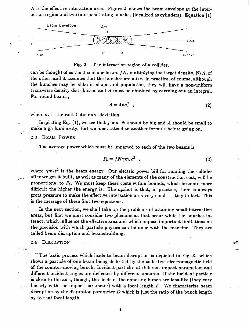
A is the effective interaction area. Figure 2 shows the beam envelope at the inter- action region and two interpenetrating bunches (idealized as cylinders). Equation (1)

Axis i ,;

- . - - 6-86 5455A2

Fig. 2. The interaction region of a collider.

can be thought of as the flux of one beam, f N, multiplying the target density, N/A, of the other, and it assumes that the bunches are alike. In practice, of course, although the bunches may be alike in shape and population, they will have a non-uniform transverse density distribution and A must be obtained by carrying out an integral. For round beams,

A= 47~7; , (2)

where or is the radial standard deviation.

- Inspecting Eq. (1)) we see that f and N should be big and A should be small to make high luminosity. But we must attend to another formula before going on.

2.3 BEAM POWER

The average power which must be imparted to each of the two beams is

Pb = jNym,c2 , (3)

where ym,c2 is the beam energy. Our electric power bill for running the collider _-.. .- . after we get it built, as well as many of the elements of the construction cost, will be c proportional to Pb. We must keep these costs within bounds, which becomes more

difficult the higher the energy is. The upshot is that, in practice, there is always great pressure to make the effective interaction area very small - tiny in fact. This is the message of these first two equations.

In the next section, we shall take up the problems of attaining small interaction areas, but first we must consider two phenomena that occur while the bunches in- teract, which influence the effective area and which impose important limitations on the precision with which particle physics can be done with the machine. They are called beam disruption and beamstrahlung.

2.4 DISRUPTION _

_ _m_

- -The basic process which leads to beam disruption is depicted .in Fig. 3. which -- shows a particle of one beam being deflected by the collective electromagnetic field

of the counter-moving bunch. Incident particles at different impact parameters and different incident angles are deflected by different amounts. If the incident particle is close to the axis, though, the fields of the opposing bunch are lens-like (they vary

. linearly with the impact parameter) with a focal length F. We characterize beam disruption by the disruption parameter D which is just the ratio of the bunch length a, to that focal length.

3

D = Q/F . (4

If D is small compared to one, there is little deflection, and the beams do not alter each other’s motions very much. On the other i ,; hand, if it- is about equal to one,

. particles entering parallel to, but well separated from, the axis, leave the back of the opposing bunch very near the axis with a rela- tively large angle. In other words, the bunch has focused those par- ticles to a point at its tail. That constitutes substantial disruption. For a round beam,

c

D= 4m,u,N

A7 ’ (5)

Typical Incident Particle

Distance aver which Particle Orbit is Bent

p= Bending Radius

Fig. 3. The motion of a typical par- ticle of one beam passing through the opposing bunch. -

where rc is the classical radius of the electron. Beam disruption is troublesome for experiments, because it can cause background events in the detector if it is not allowed for. The disrupted beam occupies a much larger volume in phase space than the incoming beam does if D is substantial in comparison to one. The detector surrounds the interaction point and has a hole running through it for the beams to pass through. This hole has to be large enough to accommodate the largest beam, and the largest beams are the disrupted beams. Otherwise, the detector would be

- . showered with back- ground. Thus beam disruption determines how close to the interaction point an event can be tracked.

On the other hand, disruption has a beneficial effect. Since each beam has a generally focusing effect on the other, the bunches are pinched, and their transverse densities are increased in the interaction region. The effective interaction area is reduced by the pinch and the luminosity is correspondingly increased.“’ (By the way, the reader is warned that the author is using the term “pinch effect” in a way which may not be exactly consistent with the usage of that term in plasma physics; however it is descriptive enough of the phenomenon to warrant its use here.) Figure 4 shows a computer simulation of the time sequence of spatial distributions of two bunches as they pinch each other and then fly apart. Both the increase in density during

-1. interaction and the disruption after it are evident in the sequence. In order to describe - tM%nhancement of luminosity by the @rich, we need to introduce the incoming area,

-- A,. This effective area corresponds to that of the topmost distributions in Fig. 4. It is the cross sectional area provided by the accelerators and their focusing systems and would be the interaction ama if the beams were sufficiently weak that they did not pinch each other. Corresponding to A, there is an incoming disruption parameter

D, = 4m,u, N

A07 - (6)

4

Now the actual luminosity can be written in terms of the unenhanced luminosity

L = fN2Ao -- A, A ’ (7)

- and we see that the enhancement is just the factor A,/A. The process has been studied by computer simulation, and curves of the enhancement of the luminosity have been obtained. An example pertinent to the SLAC Linear Collider is shown in . Fig. 5.

I I I I I

‘i

. . . . . . ;;.,,* a. :.,;“r;y;.:..:.

0

:,:;p L * ‘i&.

-I

; f;;$y -@Y.::. 3 :-..:.: ,+.& ,AJ?;+ . ‘~,‘.-CI,.C... . :, ”

e+-

- II . . . . . . . . . . . . . . 0 .;’ : :..

-I e+- -e-

I - . . a.. ..: O-

-l -

I I I I I

. . I _

O- -l - _-.. - .

c I I I I I

-5 0 5 7 /r-r.

r-80 -’ ‘V 18116.11

Fig. 4. Computer simulated collision of intense relativistic beams illustrating the pinch effect. From Hollebeeck.

8

e 86

E

5 k4

!5 r”

:2 2 z w

0

cxl (mrod)

0.25

I I

0 I 2 3 6-86 5455A5 D I SRUPTION PARAMETER Do

Fig. 5. The enhancement of luminosity, A,/A, as a func- tion of the incoming disruption parameter, D, (from Ref. 8).

As an alternative approach to computer simulation, the interpenetrating bunches may be considered-as a relativistic neutral plasma whose plasma instabilities can be calculated. lo1 From such studies, we conclude that values of D, up to 10 should be comfortably stable and usable. Perhaps even larger values are permitted, but they do not promise increased luminosity enhancement according to Fig. 5.

2.5 BEAMSTRAHLUN~ _ -1. Beamstrahlung is the emission of-acceleration radiation by the individual parti-

-- cles as a result of the collective electromagnetic fields of the opposing bunches passing them. Since the acceleration is almost perpendicular to the particle velocity, beam- strahlung is often treated as synchrotron radiation in the bunch field. It is distin- guished from beam-beam bremsstrahlung which considers only close particle-particle encounters that give rise to emissions of photons having energies comparable to the particle energies. Beamstrahlung may be regarded as considering only comparatively distant encounters where the fields of many particles are superimposed.

5

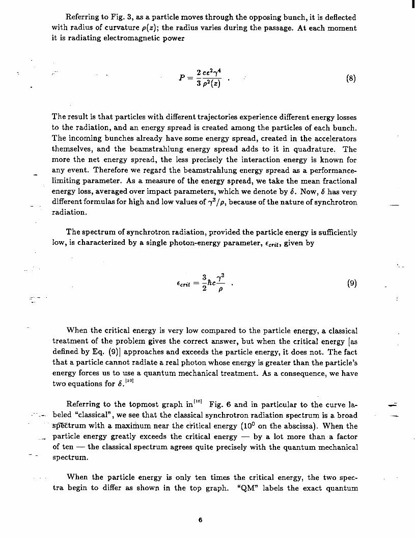
Referring to Fig. 3, as a particle moves through the opposing bunch, it is deflected with radius of curvature p(z); the radius varies during the passage. At each moment it is radiating electromagnetic power

,; -. -. p = zce2+ . ; 3 P2(4 (8)

The result is that particles with different trajectories experience different energy losses to the radiation, and an energy spread is created among the particles of each bunch. The incoming bunches already have some energy spread, created in the accelerators themselves, and the beamstrahlung energy spread adds to it in quadrature. The more the net energy spread, the less precisely the interaction energy is known for any event. Therefore we regard the beamstrahlung energy spread as a performance- limiting parameter. As a measure of the energy spread, we take the mean fractional energy loss, averaged over impact parameters, which we denote by 6. Now, 6 has very different formulas for high and low values of r3/p, because of the nature of synchrotron ._ - radiation.

The spectrum of synchrotron radiation, provided the particle energy is sufficiently low, is characterized by a single photon-energy parameter, ccrit, given by

3 r3 E,,it = p- . P

c

(9)

When the critical energy is very low compared to the particle energy, a classical treatment of the problem gives the correct answer, but when the critical energy [as defined by Eq. (9)] app roaches and exceeds the particle energy, it does not. The fact that a particle cannot radiate a real photon whose energy is greater than the particle’s energy forces us to use a quantum mechanical treatment. As a consequence, we have two equations for 6. ‘lo1

Referring to the topmost graph in”” Fig. 6 and in particular to the curve la- _ _T_ beled “classical”, we see that the classical synchrotron radiation spectrum is a broad

- spxtrum with a maximum near the c-iltical energy (10’ on the abscissa). When the

G --

- particle energy greatly exceeds the critical energy - by a lot more than a factor of ten - the classical spectrum agrees quite precisely with the quantum mechanical spectrum.

When the particle energy is only ten times the critical energy, the two spec- tra begin to differ as shown in the top graph. “QM” labels the exact quantum

6

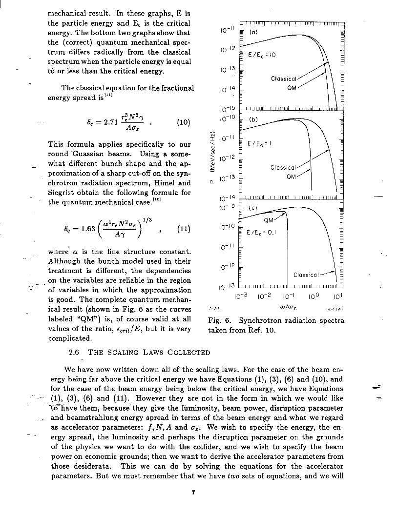
mechanical result. In these graphs, E is the particle energy and E, is the critical energy. The bottom two graphs show that the (correct) quantum mechanical spec- trum differs radically from the classical spectrum when the particle energy is equal t% or less than the critical energy.

. The classical equation for the fractional

energy spread is “‘I

r;N27 6, = 2.71 - .

Au, (10)

This formula applies specifically to our round ‘Guassian beams. Using a some- what different bunch shape and the ap- proximation of a sharp cut-off on the syn- chrotron radiation spectrum, Himel and Siegrist obtain the following formula for - the quantum mechanical case.“”

6, = 1.63 ( a4rg20z)1’3 , (11) to-‘0

. . where CY is the fine structure constant. Although the bunch model used in their treatment is different, the dependencies

-. .- on the variables are reliable in the region . c of variables in which the approximation is good. The complete quantum mechan- ical result (shown in Fig. 6 as the curves labeled “QM”) is, of course valid at all values of the ratio, +it/E, but it is very complicated.

r” .10-‘1 \

$ 10-12

r”

a 10-13

I o-3 10-2 10-I too IO’

2-85 w/u, 5043A 1

Fig. 6. Synchrotron radiation spectra taken from kef. 10.

2.6 THE SCALING LAWS COLLECTED

We have now written down all of the scaling laws. For the case of the beam en- ergy being far above the critical energy we have Equations (l), (3)) (6) and (lo), and for the case of the beam energy being below the critical energy, we have Equations

---A=. (l), (3), (6) and (11). H owever they are not in the form in which we would like - toTave them, because’ they give the Iuminosity, beam power, disruption parameter

- and beamstrahlung energy spread in terms of the beam energy and what we regard as accelerator parameters: f, N, A and a,. We wish to specify the energy, the en- ergy spread, the luminosity and perhaps the disruption parameter on the grounds of the physics we want to do with the collider, and we wish to specify the beam power on economic grounds; then we want to derive the accelerator parameters from those desiderata. This we can do by solving the equations for the accelerator parameters. But we must remember that we have two sets of equations, and we will

7

not know which set is valid until we know the critical energy of the beamstrahlung - which we will not know until we have the equations solved. We would have only one set of equations and no such dilemma if we had used the complicated quantum mechanical result for 6 (which would, in that case, need no subscript). What we can do with the equations we have is to solve both sets. Then for any given case, we must check, by calculating cerit/E, whether either set is valid. For this purpose we combine Eq. (9) with Eq.(4) and a little geometry in Fig. 3 to get

. SC 3 X,A+Dy2

E 47912 a; ' (12)

where X, is the Compton wavelength. The two sets of equations for the accelerator parameters are as follows.

Classical (c,,it < E)

1 - A = 2.71(4~)

f = 2.71(4~)

a’ = k ( reZetiL)

Quantum (~,,it > E) -. .- . -.

(13)

(14

(15)

(16) -

_. -1. (16) ; -

-- Now that we have put the scaling laws in a convenient form, let us fix these ideas in our minds by working through a couple of examples. First we shall consider the SLAC Linear Collider (SLC), the only extant (or nearly extant) specimen. Its objective specifications are as follows.

E = 50GeV,

Pb = 0.072 MW,

L = 6 x 103’ cmw2 s-l , D = 2.5, 6 = 0.0019.

We try the “Classical” equations first, and the results are -

f = 181 Hz, A = 7.4 x 10T8 cm2, ,; -. -.

. N = 5 x lOlo, UZ = 0.10 cm.

When these ‘numbers are used in Eq. (12), th e classical case proves to be the valid one. These are the accelerator parameters given by the equations , but one of them, A, is not the transverse bunch area that the collider system delivers to the interaction region; it is rather the pinched area. Instead of A, the accelerator builder needs to know A,,, and to get it, he must find values of A, and D, which correspond to A and D. to do this, he uses the curves of Fig. 5 and the relation A/A, = D/D,. When this is done, it turns out that D, is about one and A, is 2.2 x 10m7 cm2.

A final remark about the SLC example: the total energy spread in the interacting bunches is some combination of the beamstrahlung energy spread and the incoming energy spread - the energy spread created in the acceleration process itself. If we - assume that both are Guassian and uncorrelated, they combine as the sum of squares. At worst, they could add. In the SLC, the energy spread due to the accelerator is intended to be f0.002 to f0.005, so it is dominant.

Now let’s do another example: that of a l-TeV collider, one which gives a mean center-of-mass energy of 2 TeV. For this machine, we choose the parameters

. E = 1 TeV, L = 1O33 OS2 s-l 9

Pb = lMW, D = 0.1, 6 = 0.3.

-ZT’-. . We have chosen a rather small value of the disruption parameter, because we antic- ipate that this collider will operate under the conditions for which the “quantum” equations will be valid, and those equations place a premium on small values of D to keep the area large and the repetition frequency low. For the same reasons, we have chosen a rather large energy spread: 0.3 - much larger than that we would expect from the accelerators. Indeed a fractional energy spread of 0.3 in the collision energies would seriously weaken experiments done with the collider. However, the spread in collision energies is not the same as the mean beam-energy spread. The rms center-of-mass energy spread amongst collisions has been treated by Yokoya”” and by Noble’“l . The fractional spread is indeed less than 0.3. It is about 0.15. This will not permit us to use the interaction energy as a strong constraint in fitting data,

_. -1. but it may be tolerable.

~- -Using these parameters in the “quantum” equations, we obtain.

f = 22,600 Hz, A = 1 7 x lo-l2 cm2 . ,

N = 2.8 x 108, 0, = 3.5 x 10m4 cm.

In this case we have used so small a disruption parameter that we can consider that A = A,, and D = D,.

9

-

These parameters are certainly beyond present practice and technology, and whether they can be achieved is under study in many laboratories. We shall address some of the problems of achieving them in subsequent sections of our study.

3. THE ATTAINMENT OF SMALL INTERACTION AREAS ,; . . _ . In order to address the problem of attaining tiny cross-sectional areas of the beams

at the interaction point, we must introduce the emittance of the beam and the beta function of the beam transport system. The emittance characterizes the organization of the beam in phase space, and the beta function characterizes the focusing properties of the transport system.

3.1 EMITTANCE

We have already referred to phase space and remarked that it is a six-dimensional space. For the purposes of this section it will prove convenient to think of transverse phase space as the four dimensional space that describes particle motion on the two transverse coordinates, and indeed, even further, to think of the two-dimensional phase space that describes the motion on one transverse &is. (See Fig. 7.) The phase space commonly used to describe particle motion in accelerators and beam- transport systems has the particle’s transverse coordinate as abscissa and the angle of the particle’s trajectory, projected on the plane of the coordinate axis and the central orbit, as ordinate. These variables are not canonically conjugate, but they prove most useful and convenient.“” We use z to denote the coordinate along the direction of motion, the coordinate called s in Ref. 15.

. . . .

--. .- . -

. - . x’or y’ . Upright Emittance - I . _ . ’ l . Ellipse at Point

.

. . . .

5455~7 (Values Typical fdr SLC) 6-86

Fig. 7. The phase space commonly used to describe particle motion in accelerators and beam-transport systems. The ellipse surrounding a fraction of the particle points represents the emittance.

10

The emittance of a beam is a measure of its concentration in phase space; the smaller the emittance, the more concentrated is the beam. Figure 7 shows a swarm of particle points in phase space, a certain fraction of them being surrounded by an ellipse. The area of the ellipse, divided by ?r, is the emittance. (Warning: some authors do not divide by z.) For different distribution functions, different fractions of the swarm are customarily chosen to define the emittance. For our Gaussian distributions, we choose the fraction to be 47%, which means that, ifthe emittance ellipse is upright, the emittance is cZ = ~~~~~ in the z-coordinate.

The use,of an ellipse in defining the emittance is motivated, in part, by a special property the ellipse possesses for the case of a drifting beam - a beam that is not being accelerated and is not radiating - in a beam-transport system which provides linear focusing forces. In that case, the emittance ellipse has the same area everywhere along the drift path, although it changes its eccentricity and orientation as we move along. The emittance is conserved.

Even if the focusing forces are not linear, Liouville’s Theorem tells us that particle points, once confined within a closed figure, must remain forever in a closed figure of the same area, although the figure does not necessarily remain an ellipse. This is a property of a system that obeys a conservative Hamiltonian.

If the beam is being accelerated in a linear accelerator, the emittance is not conserved. It shrinks, and it shrinks in a simple way. The emittance in each transverse coordinate varies inversely with the particle energy. In the absence of transverse focusing forces, it is easy to see qualitatively why some damping should occur. The accelerating force is purely longitudinal, so the transverse momentum is constant and the transverse velocity goes down as 7 goes up.

Since we are concerned with linear accelerators, we shall find it useful to define the normalized emittance

ef& = C7 . (20) - _..~._ . - The normalized emittance will remain constant throughout acceleration provided ac- celerating forces and linear focusing forces are the only ones that need be considered.

3.2 THE BETA FUNCTION

The beta function characterizes the transverse focusing provided by the beam transport system. There is a beta function for each transverse coordinate: pZ and &,. The beta function has been taken over to linear-collider use from storage-ring practice and from general “round” accelerator theory, where it appears as the mod- ulating function of a WKB solution of the harmonic oscillator equation with varying wavelength.“” In such a solution, the transverse coordinate, say z, is given by 4

,- _Y_

-.- z(z) = d?.(z) cos[&(z) + b] , (21) ---

~ - where a and b are arbitrary constants and

- _ b(z) = / g .

(I have used a slightly different definition of & than that of Ref. 15, but one in common use.) Since a beam consists of many particles, each with its own a and

11

_-..._ . -

b, p1i2 describes the envelope of the beam’s transverse motion (provided there is no momentum dispersion - the case in a linear accelerator). Where p is small, the beam is thin; where /3 is large, the beam is fat. In terms of the emittance,

4%) = [~zPz(~)]“2 (22) ,; . . _ and similarly for y. We design the optics of the final focusing system of a linear collider so as to have no dispersion at the interaction point so that dispersion will not add to the lateral dimensions of the beam. Thus the spot size is just proportional to /3 l/2 there, and we must make p as small as possible to get a small interaction area. Assuming that cZ = Q, = E, a round beam requires & = & = p*. The superscript star indicates values at the interaction point. Now we can write the incoming effective interaction area

A, = 4&* = 47rcnp*

7 - (23)

As we have seen, A, must be very small, and therefore one of our chief tasks in building a collider is to make both the emittances and the interaction-point beta functions as small as they can be made. The measures we take to secure and to maintain small emittances will be discussed later.

There are limits on how small the beta functions can be made. The limits arise from chromatic aberrations. In a particle-optical system, momentum is the analog of frequency in a light-optical system, and the dependence of the focal length of a quadrupole magnet on momentum is the analog of chromatic aberration. Figure 8 shows a parallel beam being focused to a waist by a lens. Particles of the central momentum, po, stay within the envelope shown, which has the algebraic form

-

\i 0 2 u(z) = u* 1+ -5 .

P’

In the case of a typical collider final focus system, L >> /3*, so

*L uok:u- . P (25)

The reader should be aware that we are using the symbol L in this section as the distance from the interaction point to the nearest lens - not as the luminosity - but the meaning should be clear from the context and no confusion should arise.

_- _Y_ Consider a particle that is at the edge of the beam envelope as it passes through - tmens and that is brought to the axis at the waist by the action of the lens. That

- particle is bent by the lens through an angle 0,/L. If the particle had a momentum (p, + Ap), it would be bent by a smaller angle as shown by the dashed line in Fig.

- - 8, the diminution of the angle being by the fraction, Ap/p,. Another way of looking at it is that the waist produced by the lens for a higher momentum is farther to the right. Different momenta yield different spot sizes at the interaction point.

The consequence of the energy spread in the incoming beam, then, is to “fuzz out” the spot at the interaction point so that the smallness of the beta function (for

12

,c-

. Envelope Po+AP

(IP)

AXIS

PO 5455A8

Fig. 8. Chromatic aberration at a waist in the beam.

the central momentum) is vitiated. In order to keep this chromatic aberration from dominating the spot size

La”!!!! = ,*Lhp < (.y L PO P* PO *

- -

For this simple system, we get the result

!2<pI PO L - (26)

Since L is the space on either side of the interaction point which is left free for detector components to be snug against the beam pipe, we cannot make it too short without interfering with the ability of the machine to do physics. This means that

-. - . making ,0* small places demands on the accelerator to keep the incoming energy spread - ’ correspondingly small. For example, if L = 3 m and p* = 1 cm, then Ap/p, < 0.3% .

This simple system does not represent the best of present technology. For example, the rather complex final focus system of the SLC does a factor of two or three better. However this simple example reveals the physical origin of the effect and estimates its magnitude reasonably well.

Now that we know about how far we can reduce p*, we can figure out how small the emittances need to be for our examples, the SLC and the l-TeV collider.

In the SLC, the beta function at the interaction point is designed to be p* = 0.5 cm. We calculated earlier that the required incoming interaction area was A, = 2.2 x 10s7 cm2. From‘Eq. (23), th en, we find that c = 3.5 x lo-lo m - rad, and 4

_- _T_ -- En - = 3.5 x 10s5 m - rad. By the way, we shall use meter-radians as the units of .-Tee--- emittance, because those are the common units in the literature of colliders.

- As an exercise, the student should work out the normalized emit- tance for the - - l-TeV collider considered earlier, assuming the incoming Ap/p, = 0.5% and choosing

a sensible value for L.

To summarize, we have seen that both the emittance and the interaction-point beta function must be made as small as possible in TeV-range colliders, and since the smallness of the beta function is limited by optical aberrations, we are left with the problem of creating very small emittances.

13

An important design restraint arises from the form of Eq. (24). The waist is only small over a longitudinal distance that is short compared to /3*. If interactions between colliding bunches take place outside this short region, they do so at decreased lateral particle density and therefore at reduced local luminosity. For example, the cross-sectional area of a beam at a longitudinal location removed one /3* from the interaction point is two times larger than that at the interaction point. The upshot is that the bunch length is restricted by the value of ip*.

a, << p* (27) This limitation has not proved to be troublesome in linear colliders designed to date.

4. DAMPING RINGS

A damping ring is a storage ring for electrons or positrons which is designed to condense its bunches in phase space and thus to decrease their emittances.

We have discussed normalized emittance, a quantity which is conserved during linear acceleration and drifting. The normalized emittance which reaches the in- teraction region of a linear collider will be just the normalized emittance that was injected into the linac, so we must inject beams with small enough values into the linacs. What determines the emittances of electron beams and positron beams? Elec- trons are obtained from electron guns, and such guns do not produce sufficiently low emittances for collider service when emitting the high currents required for collider service.“’ Positrons are usually collected from the electromagnetic shower produced in a heavy-metal target which has been struck by a bunch of high-energy electrons. The resulting distribution in transverse phase space is very broad and the emittances are high - much higher than those from electron guns. Consequently, both electrons and positrons must be “cooled” in damping rings.

-

4.1 THE DAMPING PROCESS AND DAMPING TIME _-..._ . In a storage ring, the particles are continually being accelerated transversely to

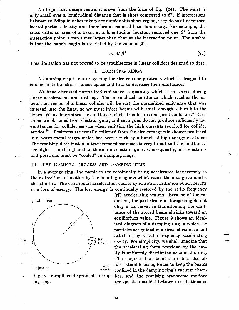
their directions of motion by the bending magnets which cause them to go around a closed orbit. The centripetal acceleration causes synchrotron radiation which results in a loss of energy. The lost energy is continually restored by the radio frequency

_- _x_

-

’ Injection

RF Cavity

6-86 5455A9

(rf) accelerating system. Because of the ra- diation, the particles in a storage ring do not obey a conservative Hamiltonian; the emit- tance of the stored beam shrinks toward an equilibrium value. Figure 9 shows an ideal- ized diagram of a damping ring in which the particles are guided in a circle of radius p and acted on by a radio frequency accelerating cavity. For simplicity, we shall imagine that the accelerating force provided by the cav- ity is uniformly distributed around the ring. The magnets that bend the orbits also af- ford lateral focusing forces to keep the beams confined in the damping ring’s vacuum cham-

Fig. 9. Simplified diagram of a damp- ber, and the resulting transverse motions ing ring. are quasi-sinusoidal betatron oscillations as

14

shown in Fig. 10. The synchrotron radiation is always emitted in the instanta- neous direction of motion (within the conical angle l/7), so the radiation reaction force is opposite to the direction of motion. But the rf force that restores the

X lost energy is always in the direction of the central orbit - the z-axis in Fig. 10. The vector diagram in Fig. 10 shows that

’ ) Z a transverse force results, which is propor- tional to the slope of the particle’s trajec- tory, k/c. That force introduces damping terms into the two transverse equations of

6-86 Frf+ p??Z&

motion.

We can estimate the magnitude of the damping rate. Assume that, in the absence

5455A10 of damping, the particles obey a simple Fig. 10. A particle executing betatron harmonic oscillator equation in the lateral oscillations in a damping ring. degrees of freedom.

0

2

z=- c z, P - (28) -

where ,6 is the average value of the beta function in the ring. Requiring power balance and using Eq. (8)) we can figure out the damping term which must be added to Eq. (28) *

e&c=P (29)

. . ensures power balance. From Fig. 10 we see

and the complete equation of motion becomes

e&

0

2

i+- ?+ c P

z=o. 7mec (31)

Solving this equation, we can get the exponential damping rate and its reciprocal, the damping time.

r=Qp2 Cre73 ’

(32)

_- An exact treatment for‘a real damping ring is somewhat more complicated,‘“’ but

eZ. this formula gives the correct magnitude of the damping times.

4; EQUILIBRIUM EMITTANCE ;.

- - If radiation damping were the only effect at play in the damping ring, the particle

motions would all die out, and the transverse emittances wo:lld shrink to zero. Of course, this does not happen. We have considered only what might be called the classical or smooth aspect of the radia- tion process and ignored its quantum nature. The radiation is emitted in quanta which cause statistical fluctuations in the motion. The particle motions are stirred up by the fluctuations and damped by the damping,

15

and after many damping times, statistical equilibrium is reached. This equilibrium state of the particle swarm has the lowest emittances attainable in the damping ring. The derivation of the equilibrium emittance is beyond the scope of these lectures, but it may be found in Ref. 16. The operation of a damping ring proceeds as follows. A bunch with transverse emittances that are too large for collider service is injected into the ring and left there for a while to damp. The emittances damp at twice the damping rate of the oscillation amplitudes.

C?(t) = Cinitiale-2t’z + equilibrium (1 - cmttir)

After many damping times, the emittance becomes equal to its equilibrium value, so the equilibrium emittance must be below the desired emittance. If it is, the first term is dominant in determining how long the particles must be allowed to damp before the bunch is extracted from the damping ring. The challenge of designing damping rings for high energy colliders is to achieve rapid damping and the smallest possible equilibrium emittances. These problems are being studied by several workers.‘“’

5. THE PRESERVATION OF EMITTANCE DURING ACCELERATION

.

After a bunch has been damped to the desired emittance in the damping ring, it is launched into the linear accelerator where it will be accelerated. Unfortunately, the linear accelerator is a hostile environment for the compact, well organized bunch and tends to disorganize it in such a way that the emittances are effectively increased and the luminosity is reduced. This process takes place through the agency of the wake field of the bunch - the electromagnetic field excited in the accelerator structure by the bunch current. topsimple terms, the wake field of the head of the bunch acts on the tail of the bunch. The wake field has components which act along the

--. .- . direction of motion of the bunch (longitudinal wakes) and components which cause transverse deflections of the particles (transverse wakes). Longitudinal wakes alter the accelerating field and lead to energy spread in the bunch. Transverse wakes cause particle motions which, in effect, increase the transverse emittance.

Although wake fields exist in all kinds of linear accelerators, they have been studied and dealt with extensively only in conventional disk-loaded microwave linac structures, and we shall confine our discussion to those.

-

5.1 WAKE FIELDS”]

Figure 11 shows two particles moving down the bore of a linac structure. Charge q at radius rg creates a’wake field which is experienced by charge e following it and

_- . ..=- displaced from the axis by r. The wake is expressed in terms of the radii at which - tIKcharges are located and the difference 4 between their azimuthal angles. It also

4 -

- depends on the longitudinal dis- tance by which e follows q. We let

- _ cr=zq-z~ , (34

and describe the longitudinal dependence of the wake by a function, W(r), called the wake potential.

16

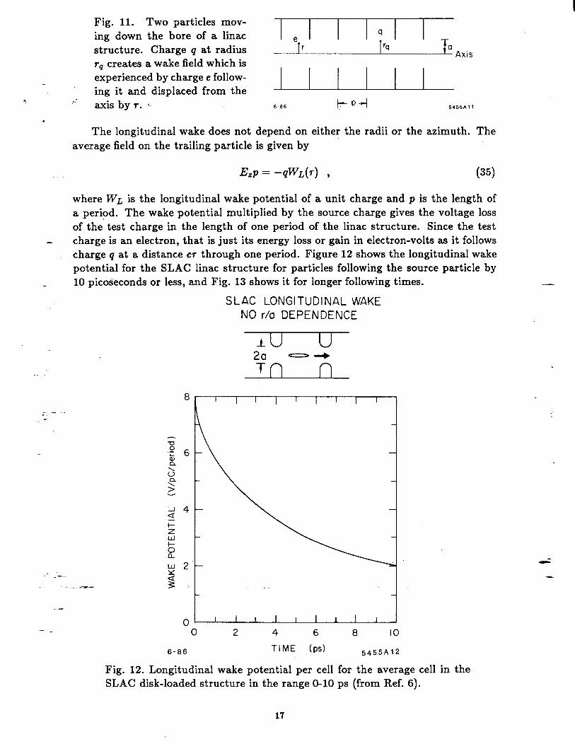
Fig. 11. Two particles mov- ing down the bore of a linac structure. Charge q at radius tq creates a wake field which is experienced by charge e follow- ing it and displaced from the

.*- axis by r. -. 6-86 kp-i 5455All

. The longitudinal wake does not depend on either the radii or the azimuth. The

average field on the trailing particle is given by

EZP = -QWId(~) 9 (35)

where WL is the longitudinal wake potential of a unit charge and p is the length of a period. The wake potential multiplied by the source charge gives the voltage loss of the test charge in the length of one period of the linac structure. Since the test charge is an electron, that is just its energy loss or gain in electron-volts as it follows charge q at a distance cr through one period. Figure 12 shows the longitudinal wake potential for the SLAC linac structure for particles following the source particle by

- 10 picoseconds or less, and Fig. 13 shows it for longer following times.

SLAC LONGITUDINAL WAKE NO r/a DEPENDENCE

8 --. .- .

_- _*_ ._ .-

J 4 a F is

i w 2 5 3 :

- _ 0

0 2 4 6 8 IO

6-86 TIME (ps) 5455A12

Fig. 12. Longitudinal wake potential per cell for the average cell in the SLAC disk-loaded structure in the range O-10 ps (from Ref. 6).

-

17

8

6

I I I I I

100 200 300 TIME (ps) 5455A13

Fig. 13. Longitudinal wake potential per cell for the SLAC structure in the range O-300 ps (from Ref. 6).

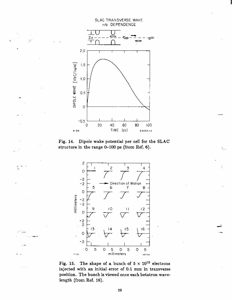
. . The transverse wake field that concerns us in collider design is called the dipole wake. It is independent of the radial position of the following charge but depends linearly on the radial position of the source particle.

_-..._ .

. j _T.

where F and 4 are unit vectors. Figure 14 shows the dipole wake potential for the SLAC structure. It is the dipole wake which tends to increase the effective emittance. It “whips the tail” of the bunch to large amplitudes of oscillation in the focusing system of the linac as shown in Fig. 15. The fact that the transverse wake field is proportional to the radial position of the source charge is the key to avoiding its deleterious effects. If the bunch is launched exactly along the axis of the accelerating structure and if the axis of the structure is perfectly aligned, the dipole wake is suppressed. These conditions are never met in practice, but they can be approached within tolerances. The stronger the focusing system of the linac,-the less is the growth of emittance, all other things being equal. More and stronger quadrupole magnets

-aGg the linac help. ’ L. -

&p = qW~(r) 2 (icos~ - &in+) ,

-

- 5.2 Two PARTICLE MODEL - -

We can make estimates of wake field effects by using a very simple model of the bunch in which the bunch current is approximated by two point charges, each having half the charge of the bunch and the second (tail) following the first (head) by 20,.

Turning first to longitudinal effects, we can calculate the wake potential at the tail due to the head using Eq. (35). Taking the total bunch population to be

18

SLAC TRANSVERSE WAKF: r/a DEPENDENCE

r

.

F 1.5 P

5 s 1.0 U W

s 3 0.5 w z i5 0

Fig. 14. Dipole wake potential per cell for the SLAC structure in the range O-100 ps (from Ref. 6).

-0.5 5 0 20 40 60 80 100

6-66 TIME (ps) 5455A14

_. .- . -

2 m s E .- - I= E

_ _T_

21, I I I I

14 [ <irec+< MO+<]

0

-2 B 7- J- 7-j -2 t --I

-2

2 13 0

L

p&l pg g

3

--

-2 3 05050505

T--83 millimeters 1577AB

Fig. 15. The shape of a bunch of 5 x 10” electrons injected with an initial error of 0.1 mm in transverse position. The bunch is viewed once each betatron wave- length (from Ref. 18).

19

5 x lOlo electrons , c7 Z = 1 cm and the total number of cells of the structure to be lo5 - numbers appropriate to the SLAC Linear Collider - we find that the total energy loss of the tail particle is about 1.1 GeV. But the head particle loses energy too - it must in order to create the wakes which leave energy behind stored in the structure. The head loses half the energy that would be lost by a test particle travelling an in- &itesimal distance behind it.‘61 According to Fig. 12, the head loses about 1.6 GeV, ‘:so the difference in energy loss, head-to-tail, is about 0.5 GeV. The student should verify these results. Fortunately, there is something that can be done to ameliorate this effect. The bunch can be placed off-crest on the accelerating wave so that the accelerating wave itself compensates the difference. Thus with the two particle model, the effect of the longitudinal wake field can be entirely cancelled at the expense of some total energy lost due to accelerating the bunch off-crest. This is not the case with a real bunch; some energy spread always arises due to the longitudinal wake, and we have seen in Section 3.2 that energy spread in the beam entering the final focus system works against small effective interaction area.

Next, let us turn to the effects of the transverse wake. In order to treat the transverse motion of particles moving down the linac, we must describe the transverse focusing system. In the SLC, the focusing system consists of a series of quadrupole magnets which may be adjusted in strength to provide a variety of beta functions to suit special requirements. For our present purpose we shall consider the case of a constant beta function - one that would be achieved by adjusting the quadrupoles’ strengths to increase in proportion to the particle energy as it increases along the accelerator. Letting subscripts 1 and 2 refer to the head and tail respectively, the equations of transverse motion are the following.‘61

-

. . x:’ + k2Xl = 0 (37)

_...._ _ - eN x; + (k + Ak)2x2 = =zl

where primes indicate differentiation with respect to z, k = l/pZ, Ak is a shift in the focusing force due to the particles having different energy and W is the dipole wake potential at the tail due to the head. The solution of the first equation is simply a free oscillation.

xl(z) = xlOeikZ (39)

If Ak 4 0, the dipole wake of the head drives the tail on resonance, and the tail executes an oscillation at (spatial) frequency k with a growing amplitude. The growth would be linear in z if it were not for the z-dependence of E, the energy of the tail

_ particle; and for our purposes, we shall take E constant at some appropriate value. - AT_ In that case, the difference in amplitude, Ax = x2 - xl, grows as follows.

~- ..~ i* - Ax I I r,NWz -=

X10 4k-i (40)

If x10 is zero, there is no growth. Growth arises because of errors in the initial conditions - the launching errors - as we saw in the sequence in Fig. 15. Even if there were no launching errors, misalignments of the linac structure itself would cause amplitude growth of this kind.

20

We may choose to operate the collider with a deliberately created difference in energy between head and tail so that Ak is not zero and the frequencies of the two particles are not exactly the same. Doing so reduces the rate of growth of amplitude. It is sometimes referred to as Landau damping. The SLC makes use of this strategy.

While the results we have obtained using the two bunch model reveal the features o-f the effects of the dipole wake quite nicely, they are not sufficiently detailed or precise to calculate ‘the tolerances required for a given collider. They do however show the qualitative feature that decreasing the beta function (increasing the focusing strength) eases the tolerances, and that remains true when Landau damping is used.

6. THE SLAC LINEAR COLLIDER

.

The SLAC Linear Collider is the first linear collider system to be undertaken. It is not strictly linear, because it seeks to use a single linac - the existing two-mile machine - as both of the linacs that would be used in the sort of linear collider described in the Introduction. Figure 16 is a schematic drawing of the SLC that shows its main systems. The electron gun and booster provide short, intense bunches of 50-MeV electrons. The first sector of the linac accelerates the electrons from the booster and also positrons from the positron source to about 1.2 GeV for injection into the damping rings. After being damped in the damping rings, bunches of electrons and positrons are accelerated simultaneously by the rest of the linac. The positron source intercepts one bunch of electrons from which it produces positrons that are transported at 200 MeV back to the first sector of the linac. The other two bunches - one of electrons and one of positrons - are accelerated to the end of the linac where they are separated to the left and right and conducted around curved beam transport paths; the arcs, which aim them at one another. Then the bunches pass through the final focus system which demagnifies them to small dimensions to produce the required effective interaction areas at the interaction point where they collide.

-

--. .- _ This scheme for using the same linac for both positrons and electrons is quite -. feasible for the energy of the SLC, 50 GeV. At that energy both the energy loss and

the emittance growth due to synchrotron radiation in the arcs are tolerable. (The energy loss is about 1 GeV.) But both the energy loss and the emittance growth rise very rapidly with energy, and the scheme is not suitable for energies much in excess of 50 GeV. Fortunately, the SLAC accelerator was readily capable of being upgraded in energy from 30 GeV to 50 GeV, and a promising experimental program, built around the Z”, made the SLC an attractive project.

The SLC operating cycle proceeds as follows. Beginning when the bunches have been damped, one positron bunch and two electron bunches are extracted from the damping rings and launched down the linac with the positron bunch leading the pro- cession. The bunches are .about twenty meters apart (60,000 picoseconds), a large

_. I _T_ enough distance to allow the wake fields to die out between bunches and to allow - a-fast-kicker-magnet pulse to rise between the second and last bunches. When the

- three bunches reach the two-thirds point of the linac, the fast kicker magnet extracts the trailing bunch of electrons which is transported to a heavy-metal target where

- - the electron bunch makes an electromagnetic shower. Positrons are selected out of the shower and accelerated to 200 MeV by the positron collection and booster sys-

_ tems and are sent back down the positron return line. When the positrons arrive at the first sector, the electron source is fired twice at the right times to establish in the first sector another procession of bunches like the one described above but in

21

,t iac

e+ Booster

Existing Linac

e+ Target

e+ Return /Line

\I

Damping Rings k \Exist ing Linac

(Sector I) e- Booster

e- Gun

r-e~ OVERALL SLC LAYOUT 4802A2

-

Fig. 16. Schematic layout of the SLAC Linear Collider. ;

_- _P_ reverse order. These are accelerated to 1.2 GeV and injected into the damping rings, -- reXring the conditions of the beginning of the cycle. Meanwhile, the positron bunch

- and the electron bunch that were not extracted at the two-thirds point of the linac have been accelerated to the end of the linac, transported around the arcs and brought

- _ into collision at the interaction point.

The SLC damping rings are designed for service at a repetition rate of 180 Hz, which means that electrons are left in the rings to damp for about 5.6 milliseconds. The positrons, which have much larger initial emittances than the electrons, are left in their damping ring for two interpulse periods or 11 milliseconds. The rings have a

22

damping time of 3 milliseconds which is achieved by operating the bending magnets at 2 Tesla for a bending radius of 2 meters. (The observant student will note that the damping time is three times longer than that given by Eq. (32). The reason is that, for a real damping ring, the equation must be corrected by a multiplicative factor of the ratio of the circumference of the ring to the sum of the lengths of the bending magnets. For the SLC damping rings, this factor is three.) The output emittance desired from Fthese rings is 1-3 x 10m8 m-rad which corresponds to a normalized emittance of 3 x 10v5 m-rad, and the equilibrium emittance is somewhat lower than that.

In the linear accelerator itself, a more powerful beam focusing and guidance system has been installed. In order to avoid emittance growth of the kind discussed in the preceding section, the axis of the beam must be maintained within a few tenths of a millimeter of the axis of the accelerating structure. The beam tends to wander from the axis because the accelerator is not straight, because of launching errors and because the rf accelerating fields steer it. The beam guidance system is modular. Each module comprises a quadrupole magnet, a high-precision beam position monitor (located in the bore of the quadrupole), and two steering magnets, one horizontal and one vertical. A quadrupole magnet assembly is shown in Fig. 17. There are about 300 of these distributed along the two-mile length of the accelerator.

C

--

_. .- . -

Fig. 17. SLC linac quadrupole magnet assembly.

REFERENCES

1. M. Tigner, Nuovo Cim. 37, p.1228 (1965).

2. B. Richter, Nucl. Inst. Methods, 136, p. 47 (1976).

- --- 4. U. Amaldi, Phys. Lett. B 61, p;- 313 (1976).

- 4. J.-E. Augustin et al., Proc. of the Workshop on the Possibilities and Limitations of Accelerators and Detectors, Fermilab, p.87 (April 1979).

5. J. Rees, “Linear Colliders-Prospects 1985,” to be published in Particle Accelerators.

23

6. P. Wilson in Laser Acceleration of Particles: Proc. of the 2nd Int. Workshop on Laser Acceleration of Particles, Los Angeles, Calif., Jan 7-18, 1985. Eds. C. Joshi and T. Katsouleas, N.Y., American Inst. Phys.,1@85, (AIP Conference Proceedings, 130). Unfortunately, the book contains several errors, and Wilson has prepared a revision of his chapter, SLAC-PUB-3674 (Rev), October 1985. It is available from the author at SLAC.

-7. V. Balaki n-and A. Skrinsky, Proc. Second ICFA ,Workshop on Possibilities and . Limitations of Accelerators and Detectors, Les Diablerets, p. 31 (October 1979).

8. R. Hollebeeck and A. Minton, Collider Note-302, SLAC internal memo, June 10, 1985.

9. R. Hollebeeck, Nucl. Inst. and Methods, 184, p. 333 (1981).

10. T. Himel and J. Siegrist, Laser Acceleration of Particles: Proc. of the 2nd Int/ Workshop on Laser Acceleration of Particles, Los Angeles, Calif., Jan. 7-18, 1985,. (AIP Conference Proceedings, 190).

11. M. Bassetti and M. Gygi-Hanney, LEP-Note 221, CERN internal memo (April 1980).

12. A. Sokolov and I. Ternov, Synchrotron Radiation, Pergamon Press, N. Y., 1968. - 13. K. Yokoya, KEK-Preprint 85-53, October 1985. (Submitted to Nucl. Instr. and

Methods.)

14. R. Noble, SLAC-PUB-3871, January 1986. (Submitted to Phys. Rev. Lett.)

15. E. Courant and H. Snyder, Ann. Phys. 3, p. 1 (1958).

16. M. Sands, uThe Physics of Electron Storage Rings”, SLAC Report 121 (1970).

. . 17. H. Wiedemann, 11th Int. Conf. on High Energy Accelerators (Birkhliuser Verlag, Base& 1980), p. 693; L. Teng, internal report LS-17, Argonne National Labo- ratory (March 1985); R. Palmer, internal report AAS Note-15 (Rev.), SLAC (February 1985); U. Amaldi, internal report CERN-EP/85-102, CERN (June - 1985).

18. R. Stiening in Physics of High Energy Particle Accelerators, Ed. M. Month, N.Y., American Inst. Phys., 1983, (AIP Conference Proceedings, 105), p. 281.

-

24

c --